Monotonicity for Multiobjective Accelerated
Proximal Gradient Methods

Abstract

Accelerated proximal gradient methods, which are also called fast iterative shrinkage-thresholding algorithms (FISTA) are known to be efficient for many applications. Recently, Tanabe et al. proposed an extension of FISTA for multiobjective optimization problems. However, similarly to the single-objective minimization case, the objective functions values may increase in some iterations, and inexact computations of subproblems can also lead to divergence. Motivated by this, here we propose a variant of the FISTA for multiobjective optimization, that imposes some monotonicity of the objective functions values. In the single-objective case, we retrieve the so-called MFISTA, proposed by Beck and Teboulle. We also prove that our method has global convergence with rate $O(1/k^{2})$, where $k$ is the number of iterations, and show some numerical advantages in requiring monotonicity.

Keywords: Multiobjective descent methods, proximal gradient methods, accelerated methods, Pareto optimality, first-order methods.

In this paper, we consider the following multiobjective optimization problem:

$$\min \quad F(x)$$ (MOP)

s.t. $$\quad x\in\mathbb{R}^{n},$$

with $F\coloneqq(F_{1},\ldots,F_{m})^{\top}$ being a vector-valued function defined by

$$F_{i}(x)\coloneqq f_{i}(x)+g_{i}(x),\quad i=1,\ldots,m,$$

where $\top$ denotes transpose, $f_{i}\colon\mathbb{R}^{n}\to\mathbb{R}$ is convex and continuously differentiable, and $g_{i}\colon\mathbb{R}^{n}\to(-\infty,\infty]$ is closed, proper and convex. Some applications for (MOP) include problems in image processing area, robust optimization and machine learning (see some examples in [4, 9, 13, 20]). In particular, if each $g_{i}$ is the indicator function of a same set, then the problem (MOP) is equivalent to a constrained optimization problem [21].

As it is well known, the simultaneous minimization of multiple objectives is done by using the concept of Pareto optimality. In this work, we are particularly interested in solving (MOP) in the Pareto sense, and by using a multiobjective descent method [11]. The research associated to multiobjective descent methods is currently increasing, as alternatives to metaheuristics [16], where no theoretical guarantee of convergence exists, and also scalarization approaches [15, 17], where unknown parameters are required. Many of these methods have been proposed in the literature, including for instance, the steepest descent [8], the Newton [7], the projected gradient [10, 14], the proximal point [5], the subgradient [6], and the conjugate gradient [18] methods.

Recently, Tanabe et al. proposed the so-called multiobjective proximal gradient method (PGM), that is specific for composite problems like (MOP) [21]. Afterwards, an accelerated version of it was also proposed [23]. Such methods are basically extensions of the ones proposed for single-valued optimization, given in [12, 1]. In particular, the accelerated version of PGM, which is often called fast iterative shrinkage-thresholding algorithm (FISTA), is used in many applications of signal processing area. While many enhancements on the scalar-valued FISTA had been proposed, most of their multiobjective counterparts had not; currently, only the original FISTA had been extended to the vector-valued context [23]. Here, we fill this gap, by proposing a variant of the multiobjective FISTA.

More specifically, the multiobjective FISTA does not guarantee monotonically decrease of the objective functions values [23]. This property is inherited from the single-objective FISTA. However, as it was demonstrated in [2], for some problems, inexact computations of subproblems may lead to a high nonmonotonicity, and even divergence. To overcome the above drawback, a monotone version of FISTA, called MFISTA, was proposed for scalar-valued problems [2]. Based on that work, here we propose a multiobjective version of MFISTA. To this end, we first clarify the notion of monotonicity in the multiobjective case. More precisely, in each iteration, we consider either the case that all objectives decrease, or when at least one objective function decreases. For the latter case, we show that the method converges globally with rate $O(1/k^{2})$, where $k$ is the number of iterations, which is the same rate of the multiobjective FISTA.

The paper is organized as follows. In Section 1, we give some notations, and remark the multiobjective proximal gradient methods, with and without acceleration. We propose our monotone version of FISTA in Section 2, and its convergence analysis is given in Section 3. Moreover, in Section 4 we show some numerical experiments. We conclude the paper in Section 5 with some final remarks.

1 Preliminaries

Let us first present some basic notations that will be used throughout the paper. For given vectors $x,y\in\mathbb{R}^{s}$, we write $x\leq y$ (resp. $x<y$) if $x_{i}\leq y_{i}$ (resp. $x_{i}<y_{i}$) for all $i=1,\dots,s$. The Euclidean norm and inner product are denoted by $\lVert\,\cdot\,\rVert$, and $\langle\cdot,\cdot\rangle$, respectively. For a given matrix $A\in\mathbb{R}^{r\times s}$, its transpose is given by $A^{\top}\in\mathbb{R}^{s\times r}$. The gradient and the subdifferential of a function $\phi\colon\mathbb{R}^{s}\to(-\infty,\infty]$ at $x\in\mathbb{R}^{s}$ are written as $\nabla\phi(x)$, and $\partial\phi(x)$, respectively.

Let us now return to problem (MOP). In the whole paper, we assume that each $f_{i}$ has a Lipschitz continuous gradient with constant $L_{i}>0$. Since we deal with various objective functions, we also define

$$L\coloneqq\max_{i\in\{1,\ldots,m\}}L_{i}.$$ (1.1)

We also denote the domain of the objective function $F$ as follows:

$$\text{dom}F\coloneqq\{x\in\mathbb{R}^{n}\mid F(x)<\infty\}.$$ (1.2)

As it is well known, in general, we may not have a point that minimizes all objectives at once. Thus, (MOP) is solved in the Pareto sense. Recall that if there is no ${\color[rgb]{0,0,0}x}\in\mathbb{R}^{n}$ such that $F(x)\leq F(x^{*})$ and $F({\color[rgb]{0,0,0}x})\neq F(x^{*})$, then $x^{*}$ is a (strongly) Pareto optimal point. Moreover, if there is no ${\color[rgb]{0,0,0}x}\in\mathbb{R}^{n}$ such that $F(x)<F(x^{*})$, then $x^{*}$ is called weakly Pareto optimal point. In this work, we are particularly interested in the this latter optimality concept.

Let us now review the multiobjective FISTA, proposed in [23], which is the base of our work. As do most descent methods, this one updates a solution in an iterative manner, and at each iteration the following subproblem is solved, with given $x,y\in\mathbb{R}^{n}$:

$$\min_{z\in\mathbb{R}^{n}}\max_{i\in\{1,\ldots,m\}}\Big{(}\left\langle\nabla f_{i}(y),z-y\right\rangle+g_{i}(z)+f_{i}(y)-F_{i}(x)\Big{)}+\frac{\ell}{2}\left\lVert z-y\right\rVert^{2},$$ (1.3)

where $\ell\geq L$. Besides the quadratic regularization term, for each $i$, it basically considers the first-order approximation of the objective, and additional terms that are important for the acceleration process. In particular, when $m=1$, this is equivalent to the subproblem used in the single-objective FISTA [1]. Moreover, the subproblem (1.3) has a unique optimal solution, because its objective function is strongly convex. Thus, denote such solution as

$$d_{\ell}(x,y):=\operatorname*{argmin}_{z\in\mathbb{R}^{n}}\max_{i\in\{1,\ldots,m\}}\Big{(}\left\langle\nabla f_{i}(y),z-y\right\rangle+g_{i}(z)+f_{i}(y)-F_{i}(x)\Big{)}+\frac{\ell}{2}\left\lVert z-y\right\rVert^{2}.$$ (1.4)

Furthermore, consider the merit function below, proposed in [22]:

$$u_{0}(x) \coloneqq\sup_{z\in\mathbb{R}^{n}}\min_{i\in\{1,\ldots,m\}}\Big{(}F_{i}(x)-F_{i}(z)\Big{)}.$$ (1.5)

Note that when $m=1$, $u_{0}(x)$ just measures the distance between $F(x)$ and the optimal objective value, which means that it is the simplest merit function for single-objective problems. The following result shows that the weak Pareto optimality can be characterized in terms of the solution of the subproblem and the above merit function.

Proposition 1.1.

Let $d_{\ell}$ and $u_{0}$ be defined by (1.4) and (1.5), respectively. Then, the following conditions are equivalent:

• $y\in\mathbb{R}^{n}$ is weakly Pareto optimal for (MOP),

• $d_{\ell}(x,y)=y$ for some $x\in\mathbb{R}^{n}$,

• $u_{0}(y)=0$.

Moreover, $u_{0}(x)\geq 0$ for all $x\in\mathbb{R}^{n}$ and the function $d_{\ell}$ is continuous.

Proof.

See [22, Theorem 3.1] and [23, Proposition 4.1]. ∎

We end this section by stating below the algorithm proposed in [23]. As we can see in [23, Theorem 5.2], this method converges globally with rate $O(1/k^{2})$, retrieving the rate of the single-objective FISTA [1, Theorem 4.4].

Algorithm 1 Multiobjective FISTA

0:  $y^{1}=x^{0}\in\text{dom}F,\ t_{1}=1,\ \ell\geq L,\ \varepsilon>0,\ k:=1$.

0:  $x^{\ast}$: weakly Pareto optimal solution

1:  while $\left\lVert d_{\ell}(x^{k-1},y^{k})-y^{k}\right\rVert\geq\varepsilon$ do

2:     $x^{k}:=d_{\ell}(x^{k-1},y^{k})$

3:     $t_{k+1}:=\Big{(}1+\sqrt{1+4t_{k}^{2}}\,\Big{)}/2$

4:     $y^{k+1}:=x^{k}+\displaystyle{\left(\frac{t_{k}-1}{t_{k+1}}\right)(x^{k}-x^{k-1})}$

5:     $k:=k+1$

6:  end while

Moreover, differently from the non-accelerated proximal gradient method [21, Sections 3.1 and 3.2], we do not necessarily have $F_{i}(x^{k})\leq F_{i}(x^{k-1})$ for each $i=1,\dots,m$ in (multiobjective) FISTA. For some instances of problems, and depending on the precision for the computation of the subproblems, the lack of monotonicity may lead to divergence. To resolve this issue, in the next section, we propose multiobjective FISTA algorithms with some monotonicity properties, that can be seem as extensions of the single-objective MFISTA [2].

2 The proposed method

Here, we establish the concept of monotonicity in multiobjective optimization, and then propose two multiobjective FISTA algorithms with monotonicity.

Definition 2.1.

Let $\{x^{k}\}$ be a sequence generated by an algorithm applied for problem (MOP). For a given iterate $k$,

• If $\displaystyle{\min_{i\in\{1,\ldots,m\}}\Big{(}F_{i}(x^{k-1})-F_{i}(x^{k})\Big{)}\geq 0}$, then we say that $F$ is strongly decreasing.

• If $\displaystyle{\max_{i\in\{1,\ldots,m\}}\Big{(}F_{i}(x^{k-1})-F_{i}(x^{k})\Big{)}\geq 0}$, then we say that $F$ is weakly decreasing.

From the definition (a), strongly decreasing $F$ at iteration $k$ means basically that $F_{i}(x^{k-1})\geq F_{i}(x^{k})$ for all $i$, i.e., all objective functions values are not increasing in that iteration. If such condition holds in all iterations, we can say that the method generates a sequence with monotonically decreasing functional values. We can also impose a stronger condition by using strict inequality in the definition (a) (which can be implied by the existence of the so-called admissible curve [19]). However, one can think that (a) and its strict version are too strong conditions. For this reason, we also consider the monotonicity defined in (b). In such case, $F$ is weakly decreasing if there exists some $j$ such that $F_{j}(x^{k-1})\geq F_{j}(x^{k})$, or in other words, at least one objective function does not increase in that iteration. However, since such $j$ may not be the same for all iterations, it is not necessarily true that some objective function decreases monotonically. In the subsequent analysis, we will see that the condition (b) allows global convergence of the method, and for such reason we state below the algorithm using only such condition.

Algorithm 2 Multiobjective MFISTA

0:  Set $y^{1}=x^{0}\in\operatorname{dom}F,\ t_{1}=1,\ \ell\geq L,\ \varepsilon>0,\ k:=1$.

0:  $x^{\ast}$: weakly Pareto optimal solution

1:  while $\left\lVert d_{\ell}(x^{k-1},y^{k})-y^{k}\right\rVert\geq\varepsilon$ do

2:     $z^{k}:=d_{\ell}(x^{k-1},y^{k})$

3:     if $\displaystyle\max_{i\in\{1,\ldots,m\}}\Big{(}F_{i}(x^{k-1})-F_{i}(z^{k})\Big{)}\geq 0$, then

4:        $x^{k}:=z^{k}$

5:     else

6:        $x^{k}:=x^{k-1}$

7:     end if

8:     $t_{k+1}:=\Big{(}1+\sqrt{1+4t_{k}^{2}}\,\Big{)}/2$

9:     $y^{k+1}:=\displaystyle{x^{k}+\left(\frac{t_{k}}{t_{k+1}}\right)(z^{k}-x^{k})+\left(\frac{t_{k}-1}{t_{k+1}}\right)(x^{k}-x^{k-1})}$

10:     $k:=k+1$

11:  end while

Comparing to Algorithm 1, we observe that a new variable $z^{k}$ is used here. From Step 3, if the monotonicity condition (in this case, from Definition 2.1(b)) holds, then we proceed as in Algorithm 1. On the other hand, if all objective functions values increase, then $y^{k}$ is updated as a convex combination with the previous point $x^{k-1}=x^{k}$ and the one computed with the subproblem, i.e., $z^{k}=d_{\ell}(x^{k-1},y^{k})$. As it can be seen in [2], when $m=1$, Algorithm 2 retrieves the single-valued MFISTA. We end this section with a simple inequality that holds in all iterations, and that will be used in the convergence analysis.

Lemma 2.2.

Let $\{x^{k}\}$ be generated by Algorithm 2. Then, for all $k\geq 0$, the following inequality holds:

$$\min_{i\in\{1,\ldots,m\}}\Big{(}F_{i}(z^{k})-F_{i}(x^{k})\Big{)}\geq 0.$$

Proof.

In each iteration of the algorithm, either $x^{k}=z^{k}$ (Step 4) or $x^{k}=x^{k-1}$ (Step 6) hold. If the former is satisfied, then trivially, $F_{i}(z^{k})-F_{i}(x^{k})=0$ for all $i=1,\ldots,m$, and so the inequality holds. On the other hand, if the latter holds, from Step 3 we have

$$\max_{i\in\{1,\ldots,m\}}\Big{(}F_{i}(x^{k-1})-F_{i}(z^{k})\Big{)}\ngeq 0,$$

which means $F_{i}(z^{k})>F_{i}(x^{k-1})$ for all $i=1,\ldots,m$. Since $x^{k}=x^{k-1}$, we also have $F_{i}(x^{k})=F_{i}(x^{k-1})$. Therefore, the claim is also true in this case. ∎

3 Convergence analysis

In this section, we will prove that the proposed multiobjective MFISTA (Algorithm 2) converges globally with rate $O(1/k^{2})$. Before this, let us recall that we assume Lipschitz continuity of the gradients $\nabla f_{i}$. Then, from (1.1), for all $p,q\in\mathbb{R}^{n}$ and $i=1,\ldots,m$, we have

$$f_{i}(p)-f_{i}(q)\leq\left\langle\nabla f_{i}(q),p-q\right\rangle+\frac{L}{2}\left\lVert p-q\right\rVert^{2}.$$

This inequality is often called descent lemma [3, Proposition A.24]. This, together with the definition of $F_{i}$, gives

$$\begin{split}F_{i}(p)-F_{i}(r)&=f_{i}(p)-f_{i}(q)+g_{i}(p)+f_{i}(q)-F_{i}(r)\\ &\leq\left\langle\nabla f_{i}(q),p-q\right\rangle+g_{i}(p)+f_{i}(q)-F_{i}(r)+\frac{L}{2}\left\lVert p-q\right\rVert^{2}\end{split}$$ (3.1)

for all $p,\ q,\ r\in\mathbb{R}^{n}$ and $i=1,\ldots,m$.

Returning to the algorithm itself, from the optimality conditions of the subproblem (1.3) (more specifically, that obtains $d_{\ell}(x^{k},y^{k+1})$), there exist $\mu(x^{k},y^{k+1})\in\partial g(d_{\ell}(x^{k},y^{k+1}))$ and $\lambda(x^{k},y^{k+1})\in\mathbb{R}^{m}$, with $\lambda_{i}(x^{k},y^{k+1})\geq 0$ for all $i=1,\dots,m$ such that

$$\sum_{i=1}^{m}\lambda_{i}(x^{k},y^{k+1})\big{(}\nabla f_{i}(y^{k+1})+\mu_{i}(x^{k},y^{k+1})\big{)}=-\ell\left(d_{\ell}(x^{k},y^{k+1})-y^{k+1}\right),$$ (3.2a)

$$\sum_{i=1}^{m}\lambda_{i}(x^{k},y^{k+1})=1,\quad\lambda_{j}(x^{k},y^{k+1})=0\quad\text{for all~{}$j\notin\mathcal{A}(x^{k},y^{k+1})$},$$ (3.2b)

where $\mathcal{A}(x^{k},y^{k+1})$ is the following set of active indices:

$$\mathcal{A}(x^{k},y^{k+1})\coloneqq \operatorname*{argmax}_{i\in\{1,\ldots,m\}}\Big{(}\left\langle\nabla f_{i}(y^{k+1}),d_{\ell}(x^{k},y^{k+1})-y^{k+1}\right\rangle$$

$$\hskip 50.0pt+g_{i}(d_{\ell}(x^{k},y^{k+1}))+f_{i}(y^{k+1})-F_{i}(x^{k})\Big{)}.$$

Furthermore, for all $k\geq 0$, we define $\sigma_{k}\colon\mathbb{R}^{n}\to[-\infty,\infty)$ as follows:

$$\sigma_{k}(z)\coloneqq\min_{i\in\{1,\ldots,m\}}\Big{(}F_{i}(x^{k})-F_{i}(z)\Big{)}.$$ (3.3)

Observe that this function is actually the objective function of the problem that defines $u_{0}(x^{k})$, given in (1.5). In the subsequent analysis, we will give an upper bound for $\sigma_{k}$, but first we establish the following technical lemma.

Lemma 3.1.

Let $\{x^{k}\}$, $\{y^{k}\}$ and $\{z^{k}\}$ be sequences generated by Algorithm 2. Then, for all $z\in\mathbb{R}^{n}$ and $k\geq 0$ we have:

• $\displaystyle{-\sigma_{k+1}(z)\geq\frac{\ell}{2}\left(\left\lVert z^{k+1}\right\rVert^{2}-\left\lVert y^{k+1}\right\rVert^{2}-2\left\langle z^{k+1}-y^{k+1},z\right\rangle\right)+\frac{\ell-L}{2}\left\lVert z^{k+1}-y^{k+1}\right\rVert^{2}}$,

• $\sigma_{k}(z)-\sigma_{k+1}(z)$
  $\>\displaystyle{\geq\frac{\ell}{2}\left(2\left\langle z^{k+1}-y^{k+1},y^{k+1}-x^{k}\right\rangle+\left\lVert z^{k+1}-y^{k+1}\right\rVert^{2}\right)+\frac{\ell-L}{2}\left\lVert z^{k+1}-y^{k+1}\right\rVert^{2}}$.

Proof.

(a) Let $z\in\mathbb{R}^{n}$ and $k\geq 0$. From the definition of $\sigma_{k+1}$ in (3.3) and using Lemma 2.2, we have

$$\begin{split}\sigma_{k+1}(z)&=\min_{i\in\{1,\ldots,m\}}\left(F_{i}(x^{k+1})-F_{i}(z)\right)\\ &\leq\min_{i\in\{1,\ldots,m\}}\left(F_{i}(z^{k+1})-F_{i}(x^{k+1})\right)+\min_{i\in\{1,\ldots,m\}}\left(F_{i}(x^{k+1})-F_{i}(z)\right)\\ &\leq\min_{i\in\{1,\ldots,m\}}\left(F_{i}(z^{k+1})-F_{i}(z)\right),\end{split}$$

where the second inequality holds because for all $p,q\in\mathbb{R}^{m}$,

$$\min_{i\in\{1,\ldots,m\}}p_{i}+\min_{i\in\{1,\ldots,m\}}q_{i}\leq\min_{i\in\{1,\ldots,m\}}(p_{i}+q_{i}).$$ (3.4)

From (3.2b), since $\lambda_{i}(x^{k},y^{k+1})\geq 0$ and $\sum_{i=1}^{m}\lambda_{i}(x^{k},y^{k+1})=1$, we obtain

$$\sigma_{k+1}(z)\leq\sum_{i=1}^{m}\lambda_{i}(x^{k},y^{k+1})\left(F_{i}(z^{k+1})-F_{i}(z)\right).$$

Now, using (3.1) with $p=z^{k+1}$, $q=y^{k+1}$ and $r=z$, we get

$$\begin{split}\sigma_{k+1}(z)&\leq\sum_{i=1}^{m}\lambda_{i}(x^{k},y^{k+1})\left(\left\langle\nabla f_{i}(y^{k+1}),z^{k+1}-y^{k+1}\right\rangle+g_{i}(z^{k+1})+f_{i}(y^{k+1})-F_{i}(z)\right)\\ &\>\quad+\frac{L}{2}\left\lVert z^{k+1}-y^{k+1}\right\rVert^{2}.\end{split}$$

Also, the convexity of $f_{i}$ and $g_{i}$ yield

$$\begin{split}&\sigma_{k+1}(z)\\ &\begin{multlined}\leq\sum_{i=1}^{m}\lambda_{i}(x^{k},y^{k+1})\left(\left\langle\nabla f_{i}(y^{k+1}),z^{k+1}-y^{k+1}\right\rangle+\left\langle\nabla f_{i}(y^{k+1}),y^{k+1}-z\right\rangle\right.\\ +\left.\left\langle\mu_{i}(x^{k},y^{k+1}),z^{k+1}-z\right\rangle\right)+\frac{L}{2}\left\lVert z^{k+1}-y^{k+1}\right\rVert^{2}\end{multlined}\leq\sum_{i=1}^{m}\lambda_{i}(x^{k},y^{k+1})\left(\left\langle\nabla f_{i}(y^{k+1}),z^{k+1}-y^{k+1}\right\rangle+\left\langle\nabla f_{i}(y^{k+1}),y^{k+1}-z\right\rangle\right.\\ +\left.\left\langle\mu_{i}(x^{k},y^{k+1}),z^{k+1}-z\right\rangle\right)+\frac{L}{2}\left\lVert z^{k+1}-y^{k+1}\right\rVert^{2}\\ &=\sum_{i=1}^{m}\lambda_{i}(x^{k},y^{k+1})\left\langle\nabla f_{i}(y^{k+1})+\mu_{i}(x^{k},y^{k+1}),z^{k+1}-z\right\rangle+\frac{L}{2}\left\lVert z^{k+1}-y^{k+1}\right\rVert^{2}.\end{split}$$

From Step 2 of Algorithm 2, we know that $d_{\ell}(x^{k},y^{k+1})=z^{k+1}$, and using (3.2a) we obtain

$$\sigma_{k+1}(z)\leq-\ell\left\langle z^{k+1}-y^{k+1},z^{k+1}-z\right\rangle+\frac{L}{2}\left\lVert z^{k+1}-y^{k+1}\right\rVert^{2}.$$

Therefore, we get

$$\begin{split}&\sigma_{k+1}(z)\\ &\leq-\frac{\ell}{2}\left(2\left\langle z^{k+1}-y^{k+1},z^{k+1}-z\right\rangle-\left\lVert z^{k+1}-y^{k+1}\right\rVert^{2}\right)-\frac{\ell-L}{2}\left\lVert z^{k+1}-y^{k+1}\right\rVert^{2}\\ &=-\frac{\ell}{2}\left(\left\lVert z^{k+1}\right\rVert^{2}-\left\lVert y^{k+1}\right\rVert^{2}-2\left\langle z^{k+1}-y^{k+1},z\right\rangle\right)-\frac{\ell-L}{2}\left\lVert z^{k+1}-y^{k+1}\right\rVert^{2},\end{split}$$

which shows that (a) holds.

(b) Once again, from the definition of $\sigma_{k}$ in (3.3) and Lemma 2.2, we have

$$\begin{split}&\sigma_{k}(z)-\sigma_{k+1}(z)\\ &\geq\min_{i\in\{1,\ldots,m\}}\left(F_{i}(x^{k})-F_{i}(z)\right)-\min_{i\in\{1,\ldots,m\}}\left(F_{i}(x^{k+1})-F_{i}(z)\right)\\ &\>\quad-\min_{i\in\{1,\ldots,m\}}\left(F_{i}(z^{k+1})-F_{i}(x^{k+1})\right)\\ &\geq\min_{i\in\{1,\ldots,m\}}\left(F_{i}(x^{k})-F_{i}(z)\right)-\min_{i\in\{1,\ldots,m\}}\left(F_{i}(z^{k+1})-F_{i}(z)\right)\\ &\geq-\max_{i\in\{1,\ldots,m\}}\left(F_{i}(z^{k+1})-F_{i}(x^{k})\right),\end{split}$$

where the second and the third inequalities hold using (3.4). From (3.1) with $p=z^{k+1}$, $q=y^{k+1}$ and $r=x^{k}$, we get

$$\begin{split}&\sigma_{k}(z)-\sigma_{k+1}(z)\\ &\begin{multlined}\geq-\max_{i=1,\ldots,m}\left(\left\langle\nabla f_{i}(y^{k+1}),z^{k+1}-y^{k+1}\right\rangle+g_{i}(z^{k+1})+f_{i}(y^{k+1})\right.\\ -\left.F_{i}(x^{k})\right)-\frac{L}{2}\left\lVert z^{k+1}-y^{k+1}\right\rVert^{2}\end{multlined}\geq-\max_{i=1,\ldots,m}\left(\left\langle\nabla f_{i}(y^{k+1}),z^{k+1}-y^{k+1}\right\rangle+g_{i}(z^{k+1})+f_{i}(y^{k+1})\right.\\ -\left.F_{i}(x^{k})\right)-\frac{L}{2}\left\lVert z^{k+1}-y^{k+1}\right\rVert^{2}\\ &\begin{multlined}=-\sum_{i=1}^{m}\lambda_{i}(x^{k},y^{k+1})\left(\left\langle\nabla f_{i}(y^{k+1}),z^{k+1}-y^{k+1}\right\rangle+g_{i}(z^{k+1})\right.\\ +\left.f_{i}(y^{k+1})-F_{i}(x^{k})\right)-\frac{L}{2}\left\lVert z^{k+1}-y^{k+1}\right\rVert^{2}\end{multlined}=-\sum_{i=1}^{m}\lambda_{i}(x^{k},y^{k+1})\left(\left\langle\nabla f_{i}(y^{k+1}),z^{k+1}-y^{k+1}\right\rangle+g_{i}(z^{k+1})\right.\\ +\left.f_{i}(y^{k+1})-F_{i}(x^{k})\right)-\frac{L}{2}\left\lVert z^{k+1}-y^{k+1}\right\rVert^{2}\\ &\begin{multlined}=-\sum_{i=1}^{m}\lambda_{i}(x^{k},y^{k+1})\left(\left\langle\nabla f_{i}(y^{k+1}),x^{k}-y^{k+1}\right\rangle+f_{i}(y^{k+1})-f_{i}(x^{k})\right)\\ -\sum_{i=1}^{m}\lambda_{i}(x^{k},y^{k+1})\left(\left\langle\nabla f_{i}(y^{k+1}),z^{k+1}-x^{k}\right\rangle+g_{i}(z^{k+1})-g_{i}(x^{k})\right)\\ -\frac{L}{2}\left\lVert z^{k+1}-y^{k+1}\right\rVert^{2},\end{multlined}=-\sum_{i=1}^{m}\lambda_{i}(x^{k},y^{k+1})\left(\left\langle\nabla f_{i}(y^{k+1}),x^{k}-y^{k+1}\right\rangle+f_{i}(y^{k+1})-f_{i}(x^{k})\right)\\ -\sum_{i=1}^{m}\lambda_{i}(x^{k},y^{k+1})\left(\left\langle\nabla f_{i}(y^{k+1}),z^{k+1}-x^{k}\right\rangle+g_{i}(z^{k+1})-g_{i}(x^{k})\right)\\ -\frac{L}{2}\left\lVert z^{k+1}-y^{k+1}\right\rVert^{2},\end{split}$$

where the first equality holds from (3.2b) and the second one is true by setting $z^{k+1}-y^{k+1}=(x^{k}-y^{k+1})+(z^{k+1}-x^{k})$. Since $f_{i}$ is convex, the first term of the above inequality is nonnegative. Moreover, from the convexity of $g_{i}$, we have:

$$\sigma_{k}(z)-\sigma_{k+1}(z)$$

$$\geq-\sum_{i=1}^{m}{\lambda_{i}(x^{k},y^{k+1})\left\langle\nabla f_{i}(y^{k+1})+\mu_{i}(x^{k},y^{k+1}),z^{k+1}-x^{k}\right\rangle}-\frac{L}{2}\left\lVert z^{k+1}-y^{k+1}\right\rVert^{2},$$

where $\mu_{i}(x^{k},y^{k+1})\in\partial g(d_{\ell}(x^{k},y^{k+1}))$. From (3.2a) the inequality below holds:

$$\begin{split}&\sigma_{k}(z)-\sigma_{k+1}(z)\\ &\geq\ell\left\langle z^{k+1}-y^{k+1},z^{k+1}-x^{k}\right\rangle-\frac{L}{2}\left\lVert z^{k+1}-y^{k+1}\right\rVert^{2}\\ &=\frac{\ell}{2}\left(2\left\langle z^{k+1}-y^{k+1},z^{k+1}-x^{k}\right\rangle-\left\lVert z^{k+1}-y^{k+1}\right\rVert^{2}\right)+\frac{\ell-L}{2}\left\lVert z^{k+1}-y^{k+1}\right\rVert^{2}\\ &=\frac{\ell}{2}\left(2\left\langle z^{k+1}-y^{k+1},y^{k+1}-x^{k}\right\rangle+\left\lVert z^{k+1}-y^{k+1}\right\rVert^{2}\right)+\frac{\ell-L}{2}\left\lVert z^{k+1}-y^{k+1}\right\rVert^{2},\end{split}$$

which completes the proof. ∎

The following result, related to stepsizes $t_{k}$, is also necessary in our analysis.

Lemma 3.2.

Let $\{t_{k}\}$ be defined by Algorithm 2. Then, for all $k\geq 1$, the following assertions hold:

$$(a)\>t_{k}\geq\frac{k+1}{2},\quad(b)\>t_{k}^{2}-t_{k+1}^{2}+t_{k+1}=0\quad\mbox{and}\quad(c)\>1-\left(\frac{t_{{\color[rgb]{0,0,0}k}}-1}{t_{k+1}}\right)^{2}\geq\frac{1}{t_{k}}>0.$$

Proof.

See [23, Lemma 4.2]. ∎

Now, we prove that for each $i=1,\dots,m$, the functional values of any sequence generated by the method do not exceed the value at the initial point. Note that this result is not trivial, because as (multiobjective) FISTA, Algorithm 2 also do not necessarily guarantee monotonicity for all the objective functions in all iterations.

Theorem 3.3.

Let $\left\{x^{k}\right\}$ be a sequence generated by Algorithm 2. Then, for all $i=1,\ldots,m$ and $k\geq 0$, we have

$$F_{i}(x^{k})\leq F_{i}(x^{0}).$$

Proof.

Let $i=1,\ldots,m$ and $k\geq 0$. Note that

$$\begin{split}F_{i}(x^{k})-F_{i}(x^{k+1})&\geq-\max_{i\in\{1,\ldots,m\}}\Big{(}F_{i}(x^{k+1})-F_{i}(x^{k})\Big{)}\\ &\geq-\max_{i\in\{1,\ldots,m\}}\Big{(}F_{i}(x^{k+1})-F_{i}(x^{k})\Big{)}+\max_{i\in\{1,\ldots,m\}}\Big{(}F_{i}(x^{k+1})-F_{i}(z^{k+1})\Big{)}\\ &\geq-\max_{i\in\{1,\ldots,m\}}\Big{(}F_{i}(z^{k+1})-F_{i}(x^{k})\Big{)},\end{split}$$

where the second inequality holds from Lemma 2.2. Also, using the same arguments from Lemma 3.1’s proof, we get

$$\begin{split}F_{i}(x^{k})-F_{i}(x^{k+1})\geq\frac{\ell}{2}\left(2\left\langle z^{k+1}-y^{k+1},y^{k+1}-x^{k}\right\rangle+\left\lVert z^{k+1}-y^{k+1}\right\rVert^{2}\right)\\ +\frac{\ell-L}{2}\left\lVert z^{k+1}-y^{k+1}\right\rVert^{2}.\end{split}$$

Since $\ell\geq L$, we can write

$$\begin{split}F_{i}(x^{k})-F_{i}(x^{k+1})&\geq\frac{\ell}{2}\left(2\left\langle z^{k+1}-y^{k+1},y^{k+1}-x^{k}\right\rangle+\left\lVert z^{k+1}-y^{k+1}\right\rVert^{2}\right)\\ &\geq\frac{\ell}{2}\left(\left\lVert z^{k+1}-x^{k}\right\rVert^{2}-\left\lVert y^{k+1}-x^{k}\right\rVert^{2}\right).\end{split}$$

From the definition of $y^{k+1}$ in Algorithm 2,

$$F_{i}(x^{k})-F_{i}(x^{k+1})\geq\frac{\ell}{2}\left(\left\lVert z^{k+1}-x^{k}\right\rVert^{2}-\left\lVert\frac{t_{k}}{t_{k+1}}(z^{k}-x^{k})+\frac{t_{k}-1}{t_{k+1}}(x^{k}-x^{k-1})\right\rVert^{2}\right).$$ (3.5)

The second term of the right-hand side of the above inequality can be written as

$$-\left\lVert\frac{t_{k}}{t_{k+1}}(z^{k}-x^{k})+\frac{t_{k}-1}{t_{k+1}}(x^{k}-x^{k-1})\right\rVert^{2}$$

$$= -\frac{1}{t_{k+1}^{2}}\left\lVert(t_{k}-1)(z^{k}-x^{k-1})+z^{k}-x^{k}\right\rVert^{2}$$

$$= -\left[\left(\frac{t_{k}-1}{t_{k+1}}\right)^{2}\left\lVert z^{k}-x^{k-1}\right\rVert^{2}+\frac{1}{t_{k+1}^{2}}\left\lVert z^{k}-x^{k}\right\rVert^{2}+2\left(\frac{t_{k}-1}{t_{k+1}^{2}}\right)\left\langle z^{k}-x^{k-1},z^{k}-x^{k}\right\rangle\right].$$

Now, let $K\coloneqq\{k\colon x^{k}=x^{k-1}\}$. Summing up $k$ from $k=1$ to $k=\hat{k}$ in (3.5), we obtain

$$\begin{split}F_{i}(x^{\hat{k}+1})\leq&\>F_{i}(x^{1})-\frac{\ell}{2}\left\lVert z^{\hat{k}+1}-x^{\hat{k}}\right\rVert^{2}-\frac{\ell}{2}\sum_{k=2}^{\hat{k}}\left[\left(1-\left(\frac{t_{k}-1}{t_{k+1}}\right)^{2}\right)\left\lVert z^{k}-x^{k-1}\right\rVert^{2}\right]\\ &{}+\frac{\ell}{2}\left(\frac{t_{1}-1}{t_{2}}\right)\left\lVert z^{1}-x^{0}\right\rVert^{2}\\ &{}+\frac{\ell}{2}\sum_{k=1,k\in K}^{\hat{k}}\left[\frac{1}{t_{k+1}^{2}}\left\lVert z^{k}-x^{k}\right\rVert^{2}+2\left(\frac{t_{k}-1}{t_{k+1}^{2}}\right)\left\langle z^{k}-x^{k-1},z^{k}-x^{k}\right\rangle\right],\end{split}$$

where the last summation follows because $k\notin K$ means $x^{k}=z^{k}$ (see Steps 4 and 6 of Algorithm 2). Moreover, the definition of $K$ and the fact that $t_{1}=1$ give

$$\begin{split}F_{i}(x^{\hat{k}+1})\leq&\>F_{i}(x^{1})-\frac{\ell}{2}\left\lVert z^{\hat{k}+1}-x^{\hat{k}}\right\rVert^{2}-\frac{\ell}{2}\sum_{k=2}^{\hat{k}}\left[\left(1-\left(\frac{t_{k}-1}{t_{k+1}}\right)^{2}\right)\left\lVert z^{k}-x^{k-1}\right\rVert^{2}\right]\\ &{}+\frac{\ell}{2}\sum_{k=1,k\in K}^{\hat{k}}\left[\left(\frac{2t_{k}-1}{t_{k+1}^{2}}\right)\left\lVert z^{k}-x^{k}\right\rVert^{2}\right]\\ \leq&\>F_{i}(x^{1})-\frac{\ell}{2}\sum_{k=2,k\in K}^{\hat{k}}\left[\left(1-\left(\frac{t_{k}-1}{t_{k+1}}\right)^{2}\right)\left\lVert z^{k}-x^{k}\right\rVert^{2}\right]\\ &{}+\frac{\ell}{2}\sum_{k=1,k\in K}^{\hat{k}}\left[\left(\frac{2t_{k}-1}{t_{k+1}^{2}}\right)\left\lVert z^{k}-x^{k}\right\rVert^{2}\right],\\ \end{split}$$

where the second inequality holds from the non-negativity of the norm, the fact that $\ell>0$, and using Lemma 3.2(c) (only for the case $k\notin K$). Simple calculations with Lemma 3.2(b) shows that

$$\begin{split}F_{i}(x^{\hat{k}+1})\leq&\>F_{i}(x^{1})-\frac{\ell}{2}\sum_{k=2,k\in K}^{\hat{k}}\frac{1}{t_{k+1}}\left\lVert z^{k}-x^{k}\right\rVert^{2}+\frac{\ell}{2t_{2}^{2}}\left\lVert z^{1}-x^{1}\right\rVert^{2}\\ \leq&\>F_{i}(x^{1})+\frac{\ell}{2t_{2}^{2}}\left\lVert z^{1}-x^{1}\right\rVert^{2}.\end{split}$$ (3.6)

Furthermore, note that $z^{1}$ is the solution of the following subproblem:

$$\min_{z\in\mathbb{R}^{n}}\max_{i\in\{1,\ldots,m\}}\{\left\langle\nabla f_{i}(x^{0}),z-x^{0}\right\rangle+g_{i}(z)-g_{i}(x^{0})\}+\frac{\ell}{2}\left\lVert z-x^{0}\right\rVert^{2}.$$

This problem is equivalent to the first iteration’s subproblem of the multiobjective proximal gradient method. From [21], the objective functions values decrease monotonically in this case. In particular, for all $i=1,\ldots,m$, we have

$$F_{i}(z^{1})\leq F_{i}(x^{0}).$$ (3.7)

Thus, $x^{1}=z^{1}$ and

$$F_{i}(x^{\hat{k}+1})\leq F_{i}(x^{1})\quad\mbox{for all }i=1,\ldots,m$$ (3.8)

holds from (3.6). Finally, from (3.7) and the fact that $x^{1}=z^{1}$ we have

$$F_{i}(x^{k})\leq F_{i}(x^{0})\quad\mbox{for all }i=1,\ldots,m,$$

and the proof is complete. ∎

We finally give an upper bound on $\sigma_{k}$ in terms of $t_{k}$ and the initial point $x^{0}$. Then, this result will be used in the main theorem, related to the complexity of Algorithm 2.

Lemma 3.4.

Let $\left\{x^{k}\right\}$ be a sequence generated by Algorithm 2. Then, for all $i=1,\ldots,m$ and $\ k\geq 0$, we have

$$t_{k}^{2}\sigma_{k}(z)\leq\frac{\ell}{2}\left\lVert x^{0}-z\right\rVert^{2}.$$ (3.9)

Proof.

Using Lemma 3.1, we obtain the following inequalities:

$$\begin{multlined}-\sigma_{k+1}(z)\geq\frac{\ell}{2}\left(\left\lVert z^{k+1}\right\rVert^{2}-\left\lVert y^{k+1}\right\rVert^{2}-2\left\langle z^{k+1}-y^{k+1},z\right\rangle\right)+\frac{\ell-L}{2}\left\lVert z^{k+1}-y^{k+1}\right\rVert^{2},\end{multlined}-\sigma_{k+1}(z)\geq\frac{\ell}{2}\left(\left\lVert z^{k+1}\right\rVert^{2}-\left\lVert y^{k+1}\right\rVert^{2}-2\left\langle z^{k+1}-y^{k+1},z\right\rangle\right)+\frac{\ell-L}{2}\left\lVert z^{k+1}-y^{k+1}\right\rVert^{2},$$ (3.11)

$$\begin{multlined}\sigma_{k}(z)-\sigma_{k+1}(z)\geq\frac{\ell}{2}\left(2\left\langle z^{k+1}-y^{k+1},y^{k+1}-x^{k}\right\rangle+\left\lVert z^{k+1}-y^{k+1}\right\rVert^{2}\right)\\ +\frac{\ell-L}{2}\left\lVert z^{k+1}-y^{k+1}\right\rVert^{2}.\end{multlined}\sigma_{k}(z)-\sigma_{k+1}(z)\geq\frac{\ell}{2}\left(2\left\langle z^{k+1}-y^{k+1},y^{k+1}-x^{k}\right\rangle+\left\lVert z^{k+1}-y^{k+1}\right\rVert^{2}\right)\\ +\frac{\ell-L}{2}\left\lVert z^{k+1}-y^{k+1}\right\rVert^{2}.$$ (3.14)

From Lemma 3.2(a), $t_{k}\geq 1$ for all $k$. We can then multiply the second inequality above by $(t_{k+1}-1)$, and add it to the first inequality. Thus, we get

$$\begin{split}&(t_{k+1}-1)\sigma_{k}(z)-t_{k+1}\sigma_{k+1}(z)\\ &\geq\frac{\ell}{2}\left(t_{k+1}\left\lVert z^{k+1}-y^{k+1}\right\rVert^{2}+2\left\langle z^{k+1}-y^{k+1},t_{k+1}y^{k+1}-(t_{k+1}-1)x^{k}-z\right\rangle\right)\\ &\>\quad+\frac{\ell-L}{2}\left(t_{k+1}\left\lVert z^{k+1}-y^{k+1}\right\rVert^{2}\right).\end{split}$$

Multiplying the above inequality by $t_{k+1}$, we further obtain

$$\begin{split}&t_{k}^{2}\sigma_{k}(z)-t_{k+1}^{2}\sigma_{k+1}(z)\\ &\geq\frac{\ell}{2}\left(\left\lVert t_{k+1}(z^{k+1}-y^{k+1})\right\rVert^{2}+2t_{k+1}\left\langle z^{k+1}-y^{k+1},t_{k+1}y^{k+1}-(t_{k+1}-1)x^{k}-z\right\rangle\right)\\ &\>\quad+\frac{\ell-L}{2}t_{k+1}^{2}\left\lVert z^{k+1}-y^{k+1}\right\rVert^{2},\end{split}$$

where the first inequality holds from Lemma 3.2(b). The Pythagoras relation

$$\left\lVert b-a\right\rVert^{2}+2\left\langle b-a,a-c\right\rangle=\left\lVert b-c\right\rVert^{2}-\left\lVert a-c\right\rVert^{2},$$

with $a\coloneqq t_{k+1}y_{k+1}$, $b\coloneqq t_{k+1}z^{k+1}$ and $c\coloneqq(t_{k+1}-1)x^{k}+z$ also shows that

$$\begin{split}&t_{k}^{2}\sigma_{k}(z)-t_{k+1}^{2}\sigma_{k+1}(z)\\ &\geq\frac{\ell}{2}\left(\left\lVert t_{k+1}z^{k+1}-(t_{k+1}-1)x^{k}-z\right\rVert^{2}-\left\lVert t_{k+1}y^{k+1}-(t_{k+1}-1)x^{k}-z\right\rVert^{2}\right)\\ &\>\quad+\frac{\ell-L}{2}t_{k+1}^{2}\left\lVert z^{k+1}-y^{k+1}\right\rVert^{2}\\ &\geq\frac{\ell}{2}\left(\left\lVert t_{k+1}z^{k+1}-(t_{k+1}-1)x^{k}-z\right\rVert^{2}-\left\lVert t_{k+1}y^{k+1}-(t_{k+1}-1)x^{k}-z\right\rVert^{2}\right).\end{split}$$

Now, define $\rho_{k}\colon\mathbb{R}^{n}\to\mathbb{R}$ as

$$\rho_{k}(z)\coloneqq\left\lVert t_{k+1}z^{k+1}-(t_{k+1}-1)x^{k}-z\right\rVert^{2}.$$ (3.15)

From the definition of $y^{k+1}$ given in Step 9 of Algorithm 2, we have

$$t_{k}^{2}\sigma_{k}(z)-t_{k+1}^{2}\sigma_{k+1}(z)\geq\frac{\ell}{2}\left\{\rho_{k}(z)-\rho_{k-1}(z)\right\}.$$

Let $\hat{k}\geq 1$. Summing the above inequality from $k=1$ to $k=\hat{k}$, we get

$$t_{1}^{2}\sigma_{1}(z)-t_{\hat{k}+1}^{2}\sigma_{\hat{k}+1}(z)\geq\frac{\ell}{2}\left\{\rho_{\hat{k}}(z)-\rho_{0}(z)\right\}.$$

Furthermore, since $\rho_{\hat{k}}(z)\geq 0$, we obtain

$$t_{\hat{k}+1}^{2}\sigma_{\hat{k}+1}(z)\leq\frac{\ell}{2}\rho_{0}(z)+t_{1}^{2}\sigma_{1}(z).$$

From Lemma 3.1 and the fact that $t_{1}=1$, we can write

$$\begin{split}t_{\hat{k}+1}^{2}\sigma_{\hat{k}+1}(z)&\leq\frac{\ell}{2}\left\lVert z^{1}-z\right\rVert^{2}+\sigma_{1}(z)\\ &\leq\frac{\ell}{2}\left\lVert z^{1}-z\right\rVert^{2}-\frac{\ell}{2}\left(2\left\langle z^{1}-y^{1},z^{1}-z\right\rangle-\left\lVert z^{1}-y^{1}\right\rVert^{2}\right)-\frac{\ell-L}{2}\left\lVert z^{1}-y^{1}\right\rVert^{2}.\end{split}$$

Because $y^{1}=x^{0}$, we have

$$\begin{split}t_{\hat{k}+1}^{2}\sigma_{\hat{k}+1}(z)&\leq\frac{\ell}{2}\left\lVert z^{1}-z\right\rVert^{2}-\frac{\ell}{2}\left(2\left\langle z^{1}-x^{0},z^{1}-z\right\rangle-\left\lVert z^{1}-x^{0}\right\rVert^{2}\right)-\frac{\ell-L}{2}\left\lVert z^{1}-x^{0}\right\rVert^{2}\\ &\leq\frac{\ell}{2}\left\lVert z^{1}-z\right\rVert^{2}-\frac{\ell}{2}\left(2\left\langle z^{1}-x^{0},z^{1}-z\right\rangle-\left\lVert z^{1}-x^{0}\right\rVert^{2}\right)\\ &=\frac{\ell}{2}\left\lVert x^{0}-z\right\rVert^{2},\end{split}$$

which shows that $t_{k}^{2}\sigma_{k}(z)\leq\ell/2\left\lVert x^{0}-z\right\rVert^{2}$, as it is claimed. ∎

Theorem 3.5.

Let $X^{*}$ be the set of weakly Pareto optimal points associated to problem (MOP), and assume that it is nonempty. For all $x\in\Omega_{F}(F(x^{0}))\coloneqq\{x\in\mathbb{R}^{n}\mid F(x)\leq F(x^{0})\}$, assume that there exists $x^{*}\in X^{*}$ such that $F(x^{*})\leq F(x)$, and define

$$\begin{split}R&\coloneqq\sup_{F^{\ast}\in F(X^{\ast}\cap\Omega_{F}(F(x^{0})))}\min_{x\in F^{-1}(\left\{F^{\ast}\right\})}\left\lVert x-x^{0}\right\rVert^{2}<\infty.\end{split}$$

Let $\left\{x^{k}\right\}$ be a sequence generated by Algorithm 2. Then, for all $k\geq 0$, we have

$$u_{0}(x^{k})\leq\frac{2\ell R}{(k+1)^{2}}.$$

Proof.

Let $k\geq 0$ and take $z\in\mathbb{R}^{n}$ arbitrarily. From the Lemma 3.2(a), we know that $t_{k}\geq(k+1)/2$. Therefore, from Lemma 3.4, we have

$$\begin{split}\sigma_{k}(z)=\min_{i=1,\ldots,m}\left(F_{i}(x^{k})-F_{i}(z)\right)\leq\frac{\ell}{2t_{k}^{2}}\left\lVert x^{0}-z\right\rVert^{2}\leq\frac{2\ell\left\lVert x^{0}-z\right\rVert^{2}}{(k+1)^{2}},\end{split}$$

and thus,

$$\sup_{F^{\ast}\in F(X^{\ast}\cap\Omega_{F}(F(x^{0})))}\min_{z\in F^{-1}(\left\{F^{\ast}\right\})}\left\{F_{i}(x^{k})-F_{i}(z)\right\}\leq\frac{2\ell R}{(k+1)^{2}}.$$

Using Theorem 3.3 and with similar arguments used in the proof of [24, Theorem 5.2], we obtain

$$u_{0}(x^{k})\leq\frac{2\ell R}{(k+1)^{2}},$$

and the proof is complete. ∎

Recalling Proposition 1.1, the above result states that the Algorithm 2 converges globally (in the weakly Pareto sense) with convergence rate $O(1/k^{2})$. Here, we use the same scalar $R$ used in the convergence analysis of multiobjective FISTA [23, Assumption 3.1], which was in turn used in the analysis of the multiobjective proximal gradient method [24, Assumption 5.1]. As stated in [24, Remark 5.3], the assumption holds trivially when $m=1$ and at least one optimal point exists, or when the level set $\Omega_{F}(F(x^{0}))$ is bounded.

Corollary 3.6.

Suppose that the same assumptions of Theorem 3.5 hold, and let $\left\{x^{k}\right\}$ be a sequence generated by Algorithm 2. Then, every accumulation point of $\left\{x^{k}\right\}$ is weakly Pareto optimal for (MOP).

Proof.

It is clear from Theorem 3.5, Proposition 1.1 and the lower-semicontinuity of the objectives. ∎

For completeness, we state above the immediate global convergence result. Naturally, if each objective function is also strictly convex, we also end up in (strongly) Pareto optimal points [7, Theorem 3.1].

4 Numerical experiments

In this section, we present some simple numerical experiments to validate the described results. We modified the code used in [23], implemented the proposed method in Python 3.7.4 and ran all the experiments on a 1.1 GHz Intel Core i5 machine with 4 cores and 8GB of memory. Besides the results of Algorithm 2, which we simply state as Weak-MFISTA here, we also show the results of the multiobjective proximal gradient method (PGM) [21], multiobjective FISTA [23], and the version of MFISTA replacing the weakly decrasing condition (Definition 2.1(b)) with the strongly decreasing one (Definition 2.1(a)), which we call Strong-MFISTA. We consider the following test problems [7], with and without objective $g$.

Problem 1. $m=3$, and

$$f_{1}(x)=\frac{1}{n^{2}}\sum_{i=1}^{n}i(x_{i}-i)^{4},\quad f_{2}(x)=\exp\left(\sum_{i=1}^{n}\frac{x_{i}}{n}\right)+\|x\|_{2}^{2},$$

$$f_{3}(x)=\frac{1}{n(n+1)}\sum_{i=1}^{n}i(n-i+1)\exp(-x_{i}),$$

$$g_{1}(x)=g_{2}(x)=g_{3}(x)=0.$$

Problem 2. $m=3$, and

$$f_{1}(x),f_{2}(x),\mbox{and }f_{3}(x)\mbox{ defined as in Problem 1},$$

$$g_{1}(x)=g_{2}(x)=g_{3}(x)=\chi_{\mathbb{R}_{+}^{n}}(x),$$

where $\chi_{\mathbb{R}_{+}^{n}}$ denotes the indicator function of the set $\mathbb{R}_{+}^{n}$.

For the above problems, we run all the algorithms $100$ times, with different initial points, which are taken in the intervals $[-2,2]^{n}$ and $[0,2]^{n}$ for Problem 1 and Problem 2, respectively. The stopping parameter $\varepsilon$ is set as $10^{-5}$, and the dimension $n$ is equal to $10$. Also, the subproblems are converted to their dual and solved with a trust-region interior point method using Scipy library. The final solutions are shown in Figure 1. In each problem, we obtain similar sets of weakly Pareto optimal points for all versions of FISTA methods.

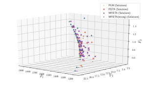
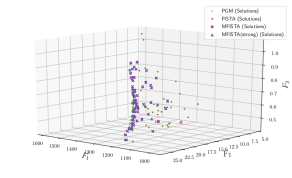
Figure 1: Pareto solutions obtained for Problem 1 (left) and Problem 2 (right)

Moreover, in Figures 2 and 3, for a given initial point, we plot $|F_{i}(x^{k})-F_{i}(x^{*})|$, where $x^{*}$ is the final (possible solution) point, at each iteration $k$. The logarithm is taken just for better visibility. As it is possible to see, for Strong-MFISTA, the objective functions are nonincreasing for all iterations. On the other hand, for Problem 1 and differently from FISTA, the Weak-MFISTA shows increase for $F_{2}$ and $F_{3}$, but decreases for at least the objective function $F_{1}$. A similar situation happens for Problem 2, but the difference between FISTA and Weak-MFISTA is small in this case.

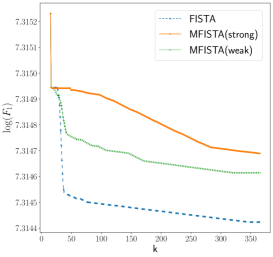
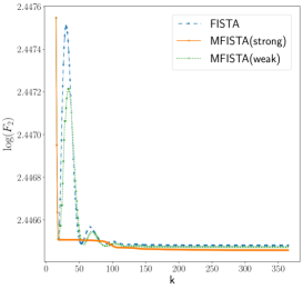
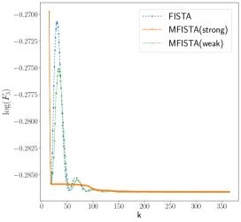
$F_{1}$ $F_{2}$ $F_{3}$

Figure 2: Functional values for Problem 1

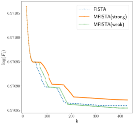
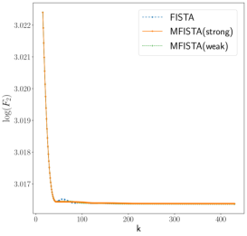
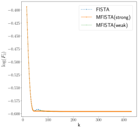
$F_{1}$ $F_{2}$ $F_{3}$

Figure 3: Functional values for Problem 2

Table 1: Average iterations and time for Problem 1

	PGM	FISTA	Weak-MFISTA	Strong-MFISTA
Iterations	606.24	206.42	203.88	202.37
Time (s)	150.85	50.41	49.78	49.52

Table 2: Average iterations and time for Problem 2

	PGM	FISTA	Weak-MFISTA	Strong-MFISTA
Iterations	981.31	276.91	277.42	303.46
Time (s)	450.40	131.39	131.99	144.09

We also check the average number of iterations and time taken for each algorithm. As it can be seem in Tables 1 and 2, all accelerated methods are better than the proximal gradient method. However, by checking also the standard deviations, we conclude that FISTA, Weak-MFISTA and Strong-MFISTA are similar in terms of iterations and time. This result is interesting, since in the single-objective case, we usually expect MFISTA to spend more time than FISTA, because of the extra computations.

Now, to observe the difference among the accelerated methods, we consider the following problem, which is the image deblurring problem [1], together with an arbitrary objective function that was only added to make the problem multiobjective.

Problem 3. $m=2$, and

$$f_{1}(x)=\|BWx-b\|^{2},\quad f_{2}(x)=0$$

$$g_{1}(x)=\lambda\|x\|_{1},\quad g_{2}(x)=\lambda\|x-1\|_{1}$$

where $\|\cdot\|_{1}$ denotes the $\ell_{1}$-norm, $B$ is the matrix representing the blur operator, $W$ is the inverse of the Haar wavelet transform, $b$ is the vectorized observed image, and $\lambda$ is the regularization parameter.

For Problem 3, we consider the $256\times 256$ cameraman test image (see [1, Section 5]) that goes through a $9\times 9$ Gaussian blur with standard deviation $4$, followed by an additional white Gaussian noise with zero-mean and standard deviation $10^{-3}$. The observed image’s wavelet transform is used as the initial point, and we set up $\lambda=2\times 10^{-5}$. Figure 4 shows the objective functions values along the iterations. For the meaningless $F_{2}$, the objective function increases with a small order in both FISTA and Weak-MFISTA. For the image deblurring related function $F_{1}$, FISTA diverges considerably during the process, Strong-MFISTA fails to converge, and Weak-MFISTA converges in few iterations.

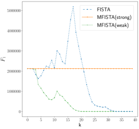
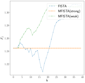
$F_{1}$ $F_{2}$

Figure 4: Functional values for Problem 3

5 Final remarks

We have proposed an alternative version of the multiobjective accelerated proximal gradient method, by considering some type of monotonicity of the objective functions. In particular, imposing a nonincrease for at least one objective function in each iteration, we obtain a method that converges globally with rate $O(1/k^{2})$. Moreover, the numerical experiments suggest that the monotonicity does not interfere in the obtained set of weakly Pareto optimal points, but can be more effective, depending on the problem. A future work will be to find interesting application problems, where the method without any monotonicity requirements can fail. Other restarting techniques should be also studied in the multiobjective case.

Acknowledgements. This work was supported by the Grant-in-Aid for Scientific Research (C) (19K11840 and 21K11769) from Japan Society for the Promotion of Science.

References

[1]Amir Beck and Marc Teboulle
“A fast iterative shrinkage-thresholding algorithm for linear inverse problems”
In SIAM Journal on Imaging Sciences2.1, 2009, pp. 183–202
[2]Amir Beck and Marc Teboulle
“Fast Gradient-Based Algorithms for Constrained Total Variation Image Denoising and Deblurring Problems”
In IEEE Transactions on Image Processing18.11, 2009, pp. 2419–2434
[4]M. Binder, J. Moosbauer, J. Thomas and B. Bischl
“Multi-objective hyperparameter tuning and feature selection using filter ensembles”
In Proceedings of the 2020 Genetic and Evolutionary Computation ConferenceAssociation for Computing Machinery, 2020, pp. 471–479
[5]H. Bonnel, A.. Iusem and B.. Svaiter
“Proximal methods in vector optimization”
In SIAM Journal on Optimization15.4, 2005, pp. 953–970
[6]J. Cruz Neto, G… Silva, O.. Ferreira and J.. Lopes
“A subgradient method for multiobjective optimization”
In Computational Optimization and Applications54.3, 2013, pp. 461–472
[7]J. Fliege, L.. Graña Drummond and B.. Svaiter
“Newton’s method for multiobjective optimization”
In SIAM Journal on Optimization20.2, 2009, pp. 602–626
[8]J. Fliege and B.. Svaiter
“Steepest Descent Methods for Multicriteria Optimization”
In Mathematical Methods of Operations Research51.3, 2000, pp. 479–494
[9]J. Fliege and R. Werner
“Robust multiobjective optimization & applications in portfolio optimization”
In European Journal of Operational Research234, 2014, pp. 422–433
[10]E.. Fukuda and L.. Graña Drummond
“On the convergence of the projected gradient method for vector optimization”
In Optimization60.8-9, 2011, pp. 1009–1021
[11]Ellen H Fukuda and Luis Mauricio Graña Drummond
“A survey on multiobjective descent methods”
In Pesquisa Operacional34.3, 2014, pp. 585–620
[12]Masao Fukushima and Hisashi Mine
“A generalized proximal point algorithm for certain non-convex minimization problems”
In International Journal of Systems Science12.8, 1981, pp. 989–1000
[13]M. Gong, M. Zhang and Y. Yuan
“Unsupervised band selection based on evolutionary multiobjective optimization for hyperspectral images”
In IEEE Transactions on Geoscience and Remote Sensing54, 2016, pp. 544–557
[14]L.. Graña Drummond and A.. Iusem
“A Projected Gradient Method for Vector Optimization Problems”
In Computational Optimization and Applications28.1, 2004, pp. 5–29
[15]J. Jahn
“Scalarization in vector optimization”
In Mathematical Programming29, 1984, pp. 203–218
[16]D.. Jones, S.. Mirrazavi and M. Tamiz
“Multi-objective meta-heuristics: An overview of the current state-of-the-art”
In European Journal of Operational Research137.1, 2002, pp. 1–9
[17]D.. Luc
“Scalarization of vector optimization problems”
In Journal of Optimization Theory and Applications55.1, 1987, pp. 85–102
[18]L.. Lucambio Pérez and L.. Prudente
“Nonlinear conjugate gradient methods for vector optimization”
In SIAM Journal on Optimization28.3, 2018, pp. 2690–2720
[19]S. Smale
“Global analysis and economics I: Pareto optimum and a generalization of Morse theory”
In Dynamical SystemsAcademic Press, 1973, pp. 531–544
[20]W. Stadler
“Multicriteria Optimization in Engineering and in the Sciences”
Springer New York, 1988
[21]Hiroki Tanabe, Ellen Hidemi Fukuda and Nobuo Yamashita
“Proximal gradient methods for multiobjective optimization and their applications”
In Computational Optimization and Applications72.2, 2019, pp. 339–361
[22]Hiroki Tanabe, Ellen Hidemi Fukuda and Nobuo Yamashita
“New merit functions for multiobjective optimization and their properties”, 2020
arXiv:2010.09333 [math.OC]
[23]Hiroki Tanabe, Ellen Hidemi Fukuda and Nobuo Yamashita
“An accelerated proximal gradient method for multiobjective optimization”
In To appear in Computational Optimization and Applications, 2023
[24]Hiroki Tanabe, Ellen Hidemi Fukuda and Nobuo Yamashita
“Convergence rates analysis of multiobjective proximal gradient method”
In Optimization Letters17, 2023, pp. 333–350
DOI: 10.1007/s11590-022-01877-7