Abstract

The total variation (TV) flow generates a scale-space representation of an image based on the TV functional. This gradient flow observes desirable features for images such as sharp edges and enables spectral, scale, and texture analysis. The standard numerical approach for TV flow requires solving multiple non-smooth optimisation problems. Even with state-of-the-art convex optimisation techniques, this is often prohibitively expensive and strongly motivates the use of alternative, faster approaches. Inspired by and extending the framework of physics-informed neural networks (PINNs), we propose the TVflowNET, a neural network approach to compute the solution of the TV flow given an initial image and a time instance. We significantly speed up the computation time by more than one order of magnitude and show that the TVflowNET approximates the TV flow solution with high fidelity. This is a preliminary report, more details are to follow.

1 Introduction

The total variation (TV) functional plays an important role in image processing. Introduced by Rudin, Fatemi, and Osher in 1992 [46] for image denoising, it has since found successful applications in noise removal [46, 43], image reconstruction [49], and segmentation [47], among many others. It is particularly suitable for image processing as it enforces piecewise constant regions and is edge-preserving. Minimising the TV functional through gradient descent yields the total variation flow [2, 3, 6], a gradient flow evolving an image based on the subdifferential of the TV functional. The TV flow gives rise to spectral, scale, and texture analysis [4, 12]. In recent years, Gilboa introduced the spectral total variation decomposition [30, 31] using the solution to the TV flow. The nonlinear spectral decomposition enables filtering and texture extraction at different scales based on the size and contrast of the structures in an image. Applications of the decomposition include image denoising [43], image fusion [7, 53, 34, 40], segmentation for biomedical images [51], and texture separation and extraction [11, 36, 24]. There exists extensive theory on the TV flow [2, 1, 3, 6, 16, 38], as well as numerical studies [27, 9, 29] and theory on the nonlinear spectral decomposition [30, 31, 32, 14, 13]. However, computing a TV flow remains challenging because the subdifferential of TV is not a singleton unless the image has no constant regions. In this case, a subgradient of minimum norm must be chosen [13]. Numerical methods amount to either modifying the gradient of the image in constant regions to make sure that the subdifferential is single-valued [27, 11] or an implicit scheme which requires solving multiple non-smooth optimisation problems [30, 31]. The first option introduces artefacts, while the second one is computationally expensive, although work on improving its efficiency continues [24, 25].

We aim to leverage recent advances in the application of deep learning to solve PDEs [26, 41, 45, 5, 42]. In particular, Raissi et al. [45] introduced the so-called physics-informed neural networks (PINNs) that approximate the PDE solution through a neural network. The loss functional consists of the 2-norms of the PDE residual and the initial and boundary conditions. The norms are discretised using sums over a random collection of points in the space-time domain. PINNs and extensions have shown promise in their application to many PDEs [44, 15]. Relating deep learning approaches to the TV flow, [33] have introduced the TVspecNET to learn the spectral TV decomposition of images. However, this work does not solve the TV flow directly. It uses supervised learning, i.e., it relies on ground truth data; furthermore, its design constrains it to fixed spectral bands of the image. Getreuer et al. [28] learn the solution to the TV flow using the so-called BLADE network, emulating the Euler method. This is also a supervised approach that relies on having ground truth solutions of the TV flow through numerical approximations. It works as a time-stepping scheme, which depends on the TV flow solution at previous time instances.

Our approach is unsupervised, which is inherent to the PINNs approach. We introduce a novel energy functional that, if minimised, yields the solution to the entire TV flow of an image up to a specific time. The main difference of our approach from standard applications of PINNs is that our network learns the solution of the TV flow from an arbitrary initial image, as opposed to standard approaches that learn the solution of a PDE with fixed initial and boundary conditions. In other words, we learn a mapping from the product of the space of images (say, $L^{2}$) and time to the space of images. Additionally, since an explicit form of the TV subgradient may be unavailable or numerically unstable, we propose a loss functional that does not rely on this explicit form and instead uses the pointwise characterisation of the TV subgradient from [8]. As a by-product, we also learn the subgradient at any instance of time

In our numerical experiments, we first show that minimising the proposed functional indeed approximates the solution to the TV flow by comparing it to time-stepping-based numerical methods - this step does not involve any neural networks. Later, we use this loss functional to approximate the TV flow solution via a neural network, the TVflowNET, in the spirit of PINNs. The approach is unsupervised and allows us to compute TV flow solutions flexibly and fast for arbitrary time instances and initial data. We show that this approach is capable of recovering the TV flow solution with high accuracy and in a computationally efficient manner. This is a preliminary report, detailed analysis of the method will follow.

2 Background

2.1 Theory

Let $\Omega\subset\mathbb{R}^{2}$ be a bounded image domain with Lipschitz continuous boundary $\partial\Omega$. We first introduce the total variation functional that is governing the flow. Following [19], we will define the functional on $L^{2}(\Omega)$, extending it with $+\infty$ whenever the supremum in the definition below does not exist.

Definition 1 (Total Variation).

Let $u\in L^{2}(\Omega)$. The total variation functional $J_{TV}:L^{2}(\Omega)\to\mathbb{R}\cup\{+\infty\}$ is given by

$$J_{TV}(u)=\begin{cases}\sup_{\lVert\varphi\rVert_{L^{\infty}}\leq 1}\int_{\Omega}u\,\textnormal{div}\,\varphi\,dx,\quad&\text{whenever this supremum is finite,}\\ +\infty&\text{otherwise.}\end{cases}$$ (1)

The supremum is taken over $\varphi\in C_{0}^{\infty}(\Omega;\mathbb{R}^{2})$ and $\lVert\varphi\rVert_{L^{\infty}}:=\sup_{x\in\Omega}\lVert\varphi(x)\rVert_{2}$.

Let $f\in L^{2}(\Omega)$ be an image. We are interested in solving the gradient flow induced by the TV functional, the so-called TV flow [2], with Neumann boundary conditions:

$$\begin{cases}u_{t}(t;x)=-p(t;x),&p(t;x)\in\partial J_{TV}(u(t)),\,\,t\in[0,\infty),\,\,x\in\Omega,\\[10.0pt] u(0;x)=f(x),&x\in\Omega,\\[10.0pt] \frac{\partial u}{\partial\eta}(t;x)=0,&t\in[0,\infty),\,\,x\in\partial\Omega,\end{cases}$$ (2)

where $\partial J_{TV}(u):=\{p\in L^{2}:J_{TV}(v)\geq J_{TV}(u)+\langle p,v-u\rangle\,\,\forall v\in L^{2}\}$ denotes the subdifferential of TV at $u\in L^{2}(\Omega)$. If $\nabla u(x)\neq 0$, the subdifferential is single-valued and given by

$$\partial J_{TV}(u)=\left\{-\operatorname{div}\left(\frac{\nabla u(x)}{\left\|\nabla u(x)\right\|_{2}}\right)\right\},\quad\nabla u(x)\neq 0.$$ (3)

If $\nabla u(x)=0$, then $\partial J_{TV}(x)$ is set-valued. The choice of Neumann boundary conditions is standard in imaging and motivated by the fact the it does not create an artificial jump at the boundary [17]. The TV flow emerges when the steepest descent method is used to minimise the TV functional (1).

The general theory of subgradient flows [10] gives us the following existence result:

Theorem 1 (Brezis [10]).

Let $f\in\overline{\mathrm{dom}(J_{TV})}$. Then there exists exactly one continuous map $u:[0,\infty)\to L^{2}$ which is Lipschitz continuous on $[\delta,\infty),\;\delta>0$ and right-differentiable on $(0,\infty)$ such that

• $u(0)=f$,

• $p(t)=\operatorname{argmin}\left\{\left\|p\right\|\colon p\in\partial J_{TV}(u(t))\right\}$ for all $t>0$,

• (2) holds for almost every $t>0$,

• $t\mapsto p(t)$ is right continuous for all $t>0$ and $t\mapsto\left\|p(t)\right\|$ is non-increasing.

As the TV flow evolves, larger piecewise constant regions in the image will develop until the image becomes constant. This happens in finite time called the extinction time [3]. These features enable scale and texture analysis and underlie the nonlinear spectral TV-decomposition [11, 4, 30, 31]. In what follows, we will describe some known numerical approaches to solving the TV flow.

2.2 Numerical approaches

The numerical solution of the TV flow (2) presents at least two major challenges. Firstly, the flow is non-linear. Secondly, the subgradient in (3) is numerically unstable in regions where $\nabla u(x)$ is small, and undefined in constant regions. The second problem is often tackled by regularising the expression in (3) as follows

$$-\operatorname{div}\left(\frac{\nabla u(x)}{\left\|\nabla u(x)\right\|_{2}+\varepsilon}\right),\quad\varepsilon>0.$$ (4)

One of the first methods that could handle the nonlinearity of (2) in a stable manner is the semi-implicit lagged diffusivity scheme [48, 22, 19]

$$\frac{u(t+dt,x)-u(t,x)}{dt}=\operatorname{div}\left(\frac{\nabla u(t+dt,x)}{\left\|\nabla u(t,x)\right\|_{2}+\varepsilon}\right),\quad dt>0,$$ (5)

which requires solving a linear elliptic equation at each iteration. Another semi-implicit scheme was proposed in [50]. A different strategy based on an auxiliary flux variable was proposed in [21] and a connection to primal-dual methods was established. [27] analyses the flow (2) with a regularised subgradient (4) as a minimal surface flow and [2] provides a semigroup analysis of the TV flow. An analysis of discretisation errors and oscillations in the TV flow was carried out in [9].

More recently, a fully implicit scheme which does not use the regularised subgradient (4) and that is unconditionally stable in the step size, was proposed in [30, 31]. An implicit Euler step in (2) is equivalent to solving the following variational denoising problem known as the ROF problem [46]:

$$u(t+dt)=\textnormal{argmin}_{v}\lVert u(t)-v\rVert_{2}^{2}+dt\,J_{TV}(v),\quad dt>0.$$ (6)

Efficient numerical schemes have been developed for solving (6), we refer to the review [20] for details. However, even these state-of-the-art methods turn out computationally expensive when (6) needs to be solved multiple times, which is what solving (2) amounts to. In the following, we will refer to solving (6) via Chambolle’s projection method [18] as the model-driven approach.

Work on improving the computational efficiency of the solution of the TV flow continues. We would like to mention the recent papers [24, 25], where Koopman’s theory of nonlinear dynamical systems is applied to the flow (2).

In this paper, we propose a different, data-driven approach based on physics-informed neural networks, which we describe in the next section. It does not rely on regularisation or time-stepping methods and is unsupervised, i.e. it does not depend on ground truth data.

3 Method

As described above, the numerical solution of the TV flow (2) for an initial image $f$ via the implicit Euler method requires solving the ROF problem (6) for each time step sequentially. Therefore, even if one is only interested in the result of the flow at time $T$, the entire flow up to time $T$ has to be evolved – this can be computationally expensive and slow. In contrast, the inference speeds of trained deep learning approaches tend to be fast. Given an initial image $f$ and a time instance $t$, we propose to approximate the solution to the TV flow $u(t)$ via a neural network, the TVFlowNET.

Our approach to solving the TV flow is inspired by the physics-informed neural networks introduced by [45]. PINNs seek to solve nonlinear PDEs of the form $u_{t}+\mathcal{N}[u]=0$ for $x\in\Omega,\,t\in[0,T]$, where $\mathcal{N}[\cdot]$ represents a nonlinear differential operator. Given randomly sampled collocation points $(t_{c}^{i};x_{c}^{i})$ for $i=1,...,N_{c}$, the network approximates the PDE solution $u(t_{c}^{i};x_{c}^{i})$. The loss functional is designed to minimise the PDE residual and enforce initial and boundary conditions given data $(t_{u}^{i},x_{u}^{i},u^{i})$ for $i=1,...,N_{u}$:

$$\mathcal{L}(u)=\frac{1}{N_{c}}\sum_{i=1}^{N_{c}}\lVert(u_{t}+\mathcal{N}[u])(t_{c}^{i},x_{c}^{i})\lVert^{2}_{2}+\frac{1}{N_{u}}\sum_{i=1}^{N_{u}}\lVert u(t_{u}^{i},x_{u}^{i})-u^{i}\rVert_{2}^{2}.$$

While PINNs have been successfully used to approximate the solutions of various PDEs [45, 44, 15], they are not directly applicable to the TV flow for the following two reasons. Firstly, a PINN is trained for a fixed initial condition and requires retraining if initial conditions change. In contrast, we seek a neural network approximating the TV flow solution for any initial image. Secondly, the explicit expression of the subgradient $-\textnormal{div}\left(\nabla u/\lvert\nabla u\rvert\right)$ in the PDE residual is not feasible due to the singularities as explained in Section 2.2.

We circumvent these difficulties via two main innovations. Firstly, we derive a new loss functional to simultaneously learn the solution $u$ and the subgradient $p$. Secondly, we use our loss functional to train a neural network that maps a given initial image, $f$, and a point in time, $t$, to the TV flow solution $u(t)$ in an unsupervised fashion.

3.1 Loss functional

To derive the loss function, we begin with the characterisation of the subgradients of the TV functional.

Theorem 2 ([8, Prop. 7]).

Let $\Omega\subset\mathbb{R}^{2}$, $u\in L^{2}(\Omega),p\in L^{2}(\Omega)$ and $J_{TV}\colon L^{2}(\Omega)\to\mathbb{R}\cup\{+\infty\}$ be as in Definition 1. Then $p\in\partial J_{TV}(u)$ if and only if

$$\begin{cases}u\in\textnormal{BV}(\Omega)\,\,\text{and}\\[7.0pt] \exists\,\varphi\in\overline{C_{0}^{\infty}(\Omega,\mathbb{R}^{2})}^{\lVert\cdot\rVert_{W^{2}(\textnormal{div})}}\,\,\text{with}\,\,\lVert\varphi\rVert_{L^{\infty}}\leq 1\,\,\text{such that}\,\,p=-\textnormal{div}\varphi,\,\,\text{and}\\[7.0pt] J_{TV}(u)=-\langle u,\text{div}\,\varphi\rangle\end{cases}$$ (7)

where $\lVert\cdot\rVert_{W^{2}(\textnormal{div})}:=\lVert\cdot\rVert_{L^{2}}^{2}+\lVert\textnormal{div}(\cdot)\rVert_{L^{2}}^{2}$.

We apply the theorem to the subdifferential in the TV flow (2) and with $p=-\textnormal{div}\varphi$ we can equivalently rephrase the PDE as follows

$$\begin{cases}u_{t}=\textnormal{div}\,\varphi,&\textnormal{in}\,\,[0,\infty)\times\Omega\\[7.0pt] |\varphi(x)|_{2}\leq 1,&x\in\Omega\\[7.0pt] J_{TV}(u)=-\langle u,\text{div}\,\varphi\rangle&\textnormal{in}\,\,[0,\infty)\times\Omega\\[7.0pt] u(0;x)=f(x),&x\in\Omega\\[7.0pt] \frac{\partial u}{\partial\eta}(t;x)=0,&t\in[0,\infty),\,\,x\in\partial\Omega\\[7.0pt] \varphi(x)=0&x\in\partial\Omega\\[7.0pt] \frac{\partial\varphi}{\partial\eta}(x)=0&x\in\partial\Omega\end{cases}$$ (8)

The boundary conditions for $\varphi$ reflect the fact that $\varphi\in\overline{C_{0}^{\infty}(\Omega,\mathbb{R}^{2})}^{\lVert\cdot\rVert_{W^{2}(\textnormal{div})}}$ and therefore both $\varphi$ and its gradient are zero at the boundary. The equivalent form (8) of the TV flow allows us to circumvent the approximation of the subgradient such as in (4). Instead, we additionally learn the diffusivity term $\varphi$ as characterised in (8) via our neural network.

We will now formulate the loss functional. Given an initial image $f$ and a time instance $t$, let $(\hat{u},\hat{\varphi})$ be the TVFlowNET’s output approximating both the solution to the TV flow $u$ and the corresponding functional $\varphi$ characterising the subgradient $\text{div}\,\varphi$ of the TV functional. We can then define the loss functional as the residuals of (8) as measured by the 2-norm:

$$\mathcal{L}=\lVert\hat{u}_{t}-\text{div}\,\hat{\varphi}\rVert_{2}^{2}+\lVert\langle\hat{u},\text{div}\,\hat{\varphi}\rangle+J_{TV}(\hat{u})\rVert_{2}^{2}+\sum_{x\in\Omega}(\lvert\hat{\varphi}(x)\rvert-1)_{+}+\lVert f-\hat{u}(0)\rVert_{2}^{2}.$$ (9)

We enforce the boundary conditions through the numerical derivation of the spatial derivatives via finite differences. We ensure that the gradient and divergence are adjoint by using forward and backward differences. We implemented the Dirichlet condition on $\varphi$ as a hard constraint by setting the spatial boundary values of the network output $\hat{\varphi}$ to 0. Finally, we can evaluate the temporal derivative of $\hat{u}$ via automatic differentiation.

3.2 Architecture Design

We design the TVFlowNET architecture following the TVspecNET [33] and DnCNN [52] approaches that use a non-contracting feed-forward convolutional neural network (CNN). [33] show that for spectral TV decomposition, these networks outperform more complex encoder-decoder type CNNs. The TVFlowNET has 8 sequential convolutional layers with 16 channels each. As activation functions, we use a combination of the rectified linear unit (ReLU) function $\sigma(x)=\max(x,0)$ [39] and softplus function $\sigma(x)=\ln(1+\exp(x))$ [54]. ReLU is used in the first layer and softplus in the subsequent ones. While ReLU is more prominent in image analysis applications [54, 52, 33], we found it not to perform as well when used on its own. As a smoothed version of the ReLU function, the softplus function is differentiable and more stable [54]. Given that the training with our loss functional involves second derivatives, this may explain the better performance of softplus compared to ReLU. However, softplus promotes images with smoothed edges; therefore, adding a single ReLU function in the neural network improved our results. Numerical experiments confirmed the advantages of the mixture of activation functions, namely combining ReLU and softplus improved the results by 9.76 PSNR points compared to solely using ReLU and by 4.93 PSNR points compared to solely using softplus.

The input of the TVFlowNET is the initial image $f$ and a randomly sampled time instance $t\in[0,1]$. We blow up the dimension of the time instance to match the size of the image and subsequently concatenate it with $f$ to form the input of the CNN. We use the network as a semi-ResNet [35] in that $\hat{u}$ is learned as an offset over a long-range residual connection from the input image, while $\hat{\varphi}$ uses no residual connection.

4 Results

Our results are twofold: First, we investigate results for minimising the designed loss functional (9) without a deep learning framework. These results serve as a baseline and show that the minimiser of the loss functional approximates a solution to the TV Flow. We expect this to be a slow optimisation, and it does not serve the goal of a computational speedup of the TV Flow solution. Secondly, we show experiments for the deep learning approach evaluated on natural images and compare the computation times to the joint space-time optimisation of the loss and, more importantly, the model-driven approach (6).

4.1 Joint space-time optimisation

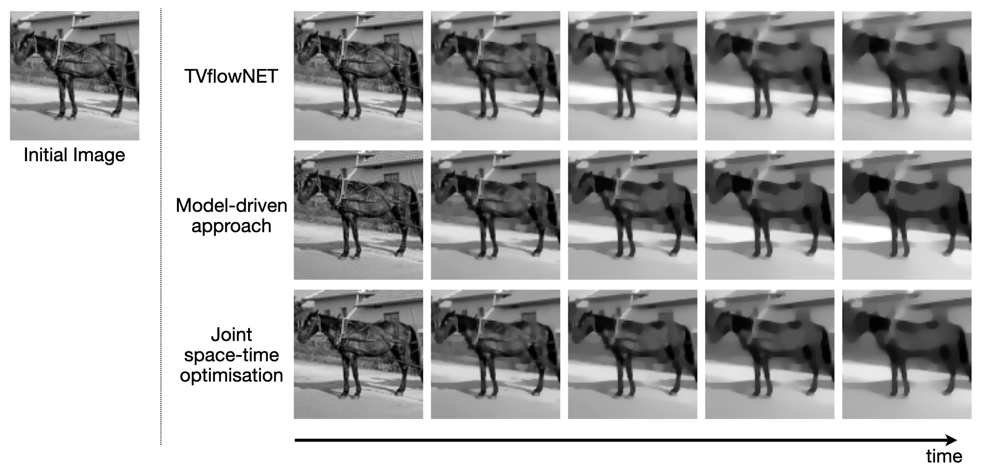
Figure 1: Visual comparison of our proposed TVFlowNET solution and the model-driven approach [31] as well as the joint time-space optimisation on an example image from the STL-10 dataset [23]. For this image, the resulting evaluation measures comparing TVflowNET and the model-driven approach are: SSIM: 0.9838, PSNR: 37.23.

We optimise the loss functional (9) jointly in space and time to form a baseline and confirm numerically that the designed loss indeed approximates the TV flow solution. That is, we do not use a neural network to approximate $u$ and $\varphi$. Instead, we initialise $u$ with the initial image $u_{ini}=f$ and $\varphi$ with a regularised form of the diffusivity term $\varphi_{ini}=\nabla u/\left(\left\|\nabla u(t,x)\right\|_{2}+\varepsilon\right)$, and we subsequently optimise over the tensor values. The optimisation is run for each input image individually and simultaneously for 50 equidistant time points in $[0,1]$. We use finite differences to evaluate the spatial and temporal derivatives in the loss functional. We employ the Adam optimiser [37] with a learning rate of $5e-3$ and iterate for $2,000$ epochs.

Comparing the results to the model-driven approach [31] in Section 2.2, we can show that the joint space-time optimisation approximates the TV flow solution with high fidelity. On a testing dataset of 200 images from the STL-10 dataset [23] we obtain a PSNR of $38.589\pm 2.157$ and an SSIM of $0.9834\pm 0.0063$. We provide a visual example of the result in Figure 1. The experiments demonstrate that our loss functional (9) recovers the TV flow images and models the evolution of the TV flow over time. It, therefore, can also be used as a baseline for the deep learning approach.

4.2 TVFlowNET

The TVflowNET is trained on the STL-10 dataset [23] containing 5000 natural images of size $96\times 96$ pixels on an NVIDIA Quadro P6000 GPU with 24 GB RAM. During training, we uniformly sample the time instances from the interval $[0,1]$ in each epoch, and we make use of automatic differentiation to evaluate the temporal derivative in the loss functional. We calculate the spatial derivatives via finite differences. Further, we use the Adam optimiser [37] with a learning rate of $5e-4$ to train the TVflowNET for $55$ epochs, after which the loss functional does not reduce significantly anymore.

We evaluate the performance of the TVflowNET against the model-driven approach and the results of the joint space-time optimisation. We can show in both cases that the neural network recovers the TV flow solution almost perfectly. A visual comparison is shown in Figure 1. The quantitative similarity measures PSNR and SSIM evaluated on a testing dataset of 200 images in Table 1 confirm the high quality of the approximated TV flow solution.

Table 1: Evaluation of the proposed TVFlowNET on 200 testing images from the STL-10 dataset [23] against the model-driven approach [31] (cf. Section 2.2) and the joint space-time optimisation (cf. Section 4.1) . Values correspond to averages over the dataset.

	SSIM	PSNR
model-driven approach	$0.9787\pm 0.004$	$37.43\pm 1.565$
joint space-time optimisation	$0.9801\pm 0.0086$	$37.58\pm 2.197$

Comparing all three approaches, we can see a clear difference in how they tread the time component. While the model-driven approach evolves the flow through time and depends on the TV flow solution of the previous time step, the joint space-time optimisation obtains the results for multiple time instances simultaneously. However, the TVflowNET is not dependent on solving the TV flow at any previous time instances but evaluates the solution $u(t)$ solely at the time of interest $t$. This makes the approach flexible and very fast in the evaluation. The improvement in computation time shown in Table 2 is of more than one order of magnitude between the model-driven approach and the TVflowNET for images of size $96\times 96$ pixels. As expected, the joint space-time optimisation approach did not yield a speedup but proved computationally more expensive. This highlights the advantage of the TVflowNET and using a trained neural network to solve the PDE.

Table 2: Computation time (in seconds) of the model driven approach evaluated on a CPU (Matlab) and on a GPU (C++/Python), of the joint space-time optimisation approach on a GPU (Python), and of the TVFlowNET evaluated on a GPU (Python). Values correspond to averages over the testing dataset of 200 images [23].

Model-driven on CPU	Model-driven on GPU	Joint space-time optimisation	TVFlowNET
$3.34\pm 0.12$	$2.491\pm 0.0066$	$17.98\pm 0.342$	$0.138\pm 0.00011$

5 Conclusion

This preliminary report introduces the TVflowNET, a neural network approximation of the TV flow via unsupervised learning for images given an initial image and a time instance. We designed a novel loss functional to circumvent the instability of the subgradient. We showed numerically that minimising the loss functional indeed recovers the TV flow solution even without a deep learning framework via joint space-time optimisation, however, at a much slower computation time. Finally, we constructed a neural network, the TVflowNET, that enables the approximation of the solution of the TV flow with very high image quality and that achieves a significant computational speedup of more than one order of magnitude compared to model-driven approaches. Further analysis of the proposed method and additional numerical studies are to follow.

TGG, YK and CBS acknowledge the support of the Cantab Capital Institute for the Mathematics of Information. TGG additionally acknowledges the support of the EPSRC National Productivity and Investment Fund grant Nr. EP/S515334/1 reference 2089694. SD is grateful for the support of the AIX-COVNET collaboration (https://covid19ai.maths.cam.ac.uk/) which is funded by Intel and the EU/EFPIA Innovative Medicines Initiative project DRAGON (101005122). YK acknowledges the support of the EPSRC (Fellowship EP/V003615/1) and the National Physical Laboratory. CBS acknowledges support from the Philip Leverhulme Prize, the Royal Society Wolfson Fellowship, the EPSRC advanced career fellowship EP/V029428/1, EPSRC grants EP/T003553/1, EP/N014588/1, the Wellcome Trust 215733/Z/19/Z and 221633/Z/20/Z, Horizon 2020 under the Marie Skodowska-Curie No. 777826 NoMADS and the Alan Turing Institute.

We also acknowledge the support of NVIDIA Corporation with the donation of two Quadro P6000 and a Tesla K40c GPU used for this research.

References

- [1] F. Andreu, C. Ballester, V. Caselles, and J. M. Mazón. The dirichlet problem for the total variation flow. Journal of Functional Analysis, 180:347–403, 3 2001.
- [2] F. Andreu, C. Ballester, V. Caselles, and J. M. Mazón. Minimizing total variation flow. Differential Integral Equations, 14:321–360, 2001.
- [3] F. Andreu, V. Caselles, J. I. Díaz, and J. M. Mazón. Some qualitative properties for the total variation flow. Journal of Functional Analysis, 188:516–547, 2 2002.
- [4] J. F. Aujol, G. Gilboa, T. Chan, and S. Osher. Structure-texture decomposition by a tv-gabor model. Lecture Notes in Computer Science (including subseries Lecture Notes in Artificial Intelligence and Lecture Notes in Bioinformatics), 3752 LNCS:85–96, 2005.
- [5] L. Bar and N. A. Sochen. Unsupervised deep learning algorithm for pde-based forward and inverse problems. CoRR, abs/1904.05417, 2019.
- [6] G. Bellettini, V. Caselles, and M. Novaga. The total variation flow in rn. Journal of Differential Equations, 184:475–525, 9 2002.
- [7] M. Benning, M. Möller, R. Z. Nossek, M. Burger, D. Cremers, G. Gilboa, and C. B. Schönlieb. Nonlinear spectral image fusion. Lecture Notes in Computer Science (including subseries Lecture Notes in Artificial Intelligence and Lecture Notes in Bioinformatics), 10302 LNCS:41–53, 2017.
- [8] K. Bredies and M. Holler. A pointwise characterization of the subdifferential of the total variation functional. arXiv preprint arXiv:1609.08918, 2016.
- [9] M. Breuss, A. Bürgel, T. Brox, T. Sonar, and J. Weickert. Numerical aspects of tv flow. Numerical Algorithms, 41:79–101, 1 2006.
- [10] H. Brezis. Operateurs maximaux monotones et semi-groupes de contractions dans les espaces de Hilbert, volume 5. Elsevier, 1973.
- [11] T. Brox and J. Weickert. A tv flow based local scale measure for texture discrimination. Lecture Notes in Computer Science (including subseries Lecture Notes in Artificial Intelligence and Lecture Notes in Bioinformatics), 3022:578–590, 2004.
- [12] T. Brox and J. Weickert. A tv flow based local scale estimate and its application to texture discrimination. Journal of Visual Communication and Image Representation, 17:1053–1073, 10 2006.
- [13] L. Bungert, M. Burger, A. Chambolle, and M. Novaga. Nonlinear spectral decompositions by gradient flows of one-homogeneous functionals. Analysis & PDE, 1 2019.
- [14] M. Burger, G. Gilboa, M. Moeller, L. Eckardt, and D. Cremers. Spectral decompositions using one-homogeneous functionals. SIAM Journal on Imaging Sciences, 9(3):1374–1408, jan 2016.
- [15] S. Cai, Z. Wang, S. Wang, P. Perdikaris, and G. E. Karniadakis. Physics-Informed Neural Networks for Heat Transfer Problems. Journal of Heat Transfer, 143(6), 04 2021.
- [16] V. Caselles, K. Jalalzai, and M. Novaga. On the jump set of solutions of the total variation flow. Rendiconti del Seminario Matematico della Università di Padova, 130:155–168, 2013.
- [17] F. Catté, P.-L. Lions, J.-M. Morel, and T. Coll. Image selective smoothing and edge detection by nonlinear diffusion. SIAM Journal on Numerical Analysis, 29(1):182–193, 1992.
- [18] A. Chambolle. An algorithm for total variation minimization and applications. Journal of Mathematical imaging and vision, 20(1):89–97, 2004.
- [19] A. Chambolle and P.-L. Lions. Image recovery via total variation minimization and related problems. Numerische Mathematik, 76(2):167–188, 1997.
- [20] A. Chambolle and T. Pock. An introduction to continuous optimization for imaging. Acta Numerica, 25:161–319, 2016.
- [21] T. F. Chan, G. H. Golub, and P. Mulet. A nonlinear primal-dual method for total variation-based image restoration. SIAM Journal on Scientific Computing, 20(6):1964–1977, 1999.
- [22] T. F. Chan and P. Mulet. On the convergence of the lagged diffusivity fixed point method in total variation image restoration. SIAM journal on numerical analysis, 36(2):354–367, 1999.
- [23] A. Coates, A. Ng, and H. Lee. An analysis of single-layer networks in unsupervised feature learning. In G. Gordon, D. Dunson, and M. Dudík, editors, Proceedings of the Fourteenth International Conference on Artificial Intelligence and Statistics, volume 15 of Proceedings of Machine Learning Research, pages 215–223, Fort Lauderdale, FL, USA, 11–13 Apr 2011. PMLR.
- [24] I. Cohen, T. Berkov, and G. Gilboa. Total-variation mode decomposition. In A. Elmoataz, J. Fadili, Y. Quéau, J. Rabin, and L. Simon, editors, Scale Space and Variational Methods in Computer Vision, pages 52–64. Springer International Publishing, 2021.
- [25] I. Cohen and G. Gilboa. Latent modes of nonlinear flows – a Koopman theory analysis. arXiv:2107.07456, 2021.
- [26] W. E and B. Yu. The deep ritz method: A deep learning-based numerical algorithm for solving variational problems. CoRR, abs/1710.00211, 2017.
- [27] X. Feng and A. Prohl. Analysis of total variation flow and its finite element approximations. ESAIM: Mathematical Modelling and Numerical Analysis, 37:533–556, 5 2003.
- [28] P. T. Getreuer, P. Milanfar, and X. Luo. Solving image pdes with a shallow network. CoRR, abs/2110.08327, 2021.
- [29] Y. Giga, M. Muszkieta, and P. Rybka. A duality based approach to the minimizing total variation flow in the space h-s. Japan Journal of Industrial and Applied Mathematics, 36:261–286, 1 2019.
- [30] G. Gilboa. A spectral approach to total variation. Lecture Notes in Computer Science (including subseries Lecture Notes in Artificial Intelligence and Lecture Notes in Bioinformatics), 7893 LNCS:36–47, 2013.
- [31] G. Gilboa. A total variation spectral framework for scale and texture analysis. SIAM Journal on Imaging Sciences, 7(4):1937–1961, jan 2014.
- [32] G. Gilboa. Nonlinear Eigenproblems in Image Processing and Computer Vision. Springer International Publishing, 2018.
- [33] T. G. Grossmann, Y. Korolev, G. Gilboa, and C.-B. Schönlieb. Deeply learned spectral total variation decomposition. In H. Larochelle, M. Ranzato, R. Hadsell, M. F. Balcan, and H. Lin, editors, Advances in Neural Information Processing Systems, volume 33, pages 12115–12126. Curran Associates, Inc., 2020.
- [34] E. Hait and G. Gilboa. Spectral total-variation local scale signatures for image manipulation and fusion. IEEE Transactions on Image Processing, 28:880–895, 2 2019.
- [35] K. He, X. Zhang, S. Ren, and J. Sun. Deep residual learning for image recognition. CoRR, abs/1512.03385, 2015.
- [36] D. Horesh and G. Gilboa. Separation surfaces in the spectral tv domain for texture decomposition. IEEE Transactions on Image Processing, 25(9):4260–4270, 2016.
- [37] D. P. Kingma and J. Ba. Adam: A method for stochastic optimization. arXiv preprint arXiv:1412.6980, 2014.
- [38] J. Kinnunen and C. Scheven. On the definition of solution to the total variation flow. Calculus of Variations and Partial Differential Equations, 61, 2 2022.
- [39] A. Krizhevsky, I. Sutskever, and G. E. Hinton. Imagenet classification with deep convolutional neural networks. In F. Pereira, C. J. C. Burges, L. Bottou, and K. Q. Weinberger, editors, Advances in Neural Information Processing Systems, volume 25. Curran Associates, Inc., 2012.
- [40] Y. Liu, R. Hou, D. Zhou, R. Nie, Z. Ding, Y. Guo, and L. Zhao. Multimodal medical image fusion based on the spectral total variation and local structural patch measurement. International Journal of Imaging Systems and Technology, 31:391–411, 3 2021.
- [41] Z. Long, Y. Lu, X. Ma, and B. Dong. PDE-net: Learning PDEs from data. In J. Dy and A. Krause, editors, Proceedings of the 35th International Conference on Machine Learning, volume 80 of Proceedings of Machine Learning Research, pages 3208–3216. PMLR, 10–15 Jul 2018.
- [42] L. Lu, P. Jin, G. Pang, Z. Zhang, and G. E. Karniadakis. Learning nonlinear operators via deeponet based on the universal approximation theorem of operators. Nature Machine Intelligence 2021 3:3, 3:218–229, 3 2021.
- [43] M. Moeller, J. Diebold, G. Gilboa, and D. Cremers. Learning nonlinear spectral filters for color image reconstruction. In 2015 IEEE International Conference on Computer Vision (ICCV), pages 289–297, 2015.
- [44] G. Pang, L. Lu, and G. E. Karniadakis. fpinns: Fractional physics-informed neural networks. SIAM Journal on Scientific Computing, 41(4):A2603–A2626, 2019.
- [45] M. Raissi, P. Perdikaris, and G. Karniadakis. Physics-informed neural networks: A deep learning framework for solving forward and inverse problems involving nonlinear partial differential equations. Journal of Computational Physics, 378:686–707, 2019.
- [46] L. I. Rudin, S. Osher, and E. Fatemi. Nonlinear total variation based noise removal algorithms. Physica D: Nonlinear Phenomena, 60:259–268, 11 1992.
- [47] M. Unger, T. Pock, W. Trobin, D. Cremers, and H. Bischof. Tvseg-interactive total variation based image segmentation. In Proceedings of British Machine Vision Conference (BMVC 2008), pages 01–02. ., 2008.
- [48] C. R. Vogel and M. E. Oman. Iterative methods for total variation denoising. SIAM Journal on Scientific Computing, 17(1):227–238, 1996.
- [49] Y. Wang, J. Yang, W. Yin, and Y. Zhang. A new alternating minimization algorithm for total variation image reconstruction. SIAM Journal on Imaging Sciences, 1(3):248–272, 2008.
- [50] J. Weickert, B. Romeny, and M. Viergever. Efficient and reliable schemes for nonlinear diffusion filtering. IEEE Transactions on Image Processing, 7(3):398–410, 1998.
- [51] L. Zeune, G. van Dalum, L. W. Terstappen, S. A. van Gils, and C. Brune. Multiscale segmentation via bregman distances and nonlinear spectral analysis. SIAM Journal on Imaging Sciences, 10(1):111–146, 2017.
- [52] K. Zhang, W. Zuo, Y. Chen, D. Meng, and L. Zhang. Beyond a gaussian denoiser: Residual learning of deep CNN for image denoising. IEEE Transactions on Image Processing, 26(7):3142–3155, July 2017.
- [53] W. Zhao, H. Lu, and D. Wang. Multisensor image fusion and enhancement in spectral total variation domain. IEEE Transactions on Multimedia, 20:866–879, 4 2018.
- [54] H. Zheng, Z. Yang, W. Liu, J. Liang, and Y. Li. Improving deep neural networks using softplus units. In 2015 International Joint Conference on Neural Networks (IJCNN), pages 1–4, 2015.