Corrections to scaling in the 3D Ising model:
a comparison between MC and MCRG results

Abstract

Corrections to scaling in the 3D Ising model are studied based on Monte Carlo (MC) simulation results for very large lattices with linear lattice sizes up to $L=3456$. Our estimated values of the correction-to-scaling exponent $\omega$ tend to decrease below the usually accepted value about $0.83$ when the smallest lattice sizes are discarded from the fits. This behavior apparently confirms some of the known estimates of the Monte Carlo renormalization group (MCRG) method, i. e., $\omega\approx 0.7$ and $\omega=0.75(5)$. We discuss the possibilities that $\omega$ is either really smaller than usually expected or these values of $\omega$ describe some transient behavior. We propose refining MCRG simulations and analysis to resolve this issue. In distinction from $\omega$, our actual MC estimations of the critical exponents $\eta$ and $\nu$ provide stable values $\eta=0.03632(13)$ and $\nu=0.63017(31)$, which well agree with those of the conformal bootstrap method, i. e., $\eta=0.0362978(20)$ and $\nu=0.6299709(40)$.

Keywords: Ising model, corrections to scaling, Monte Carlo simulation, Parallel Wolff algorithms, Very large lattices, Scaling analysis, Monte Carlo renormalization group, Conformal bootstrap

1 Introduction

The 3D Ising model is one of the most extensively studied three-dimensional systems. Focusing on the non-perturbative methods, one has to mention numerous Monte Carlo (MC) simulations – see e. g. [1, 2, 3, 4, 5] and references therein, as well as Monte Carlo renormalization group (MCRG) studies [6, 7, 8] of the 3D Ising model. High- and low-temperature series expansions [9, 10] are other numerical approaches, dealing directly with the Ising model. The large mass expansion [11] can be mentioned as an alternative to the high temperature expansion. There are many different analytical and numerical approaches, including the perturbative [20, 21, 22, 23, 24, 25, 26, 27] and the nonperturbative renormalization group (RG) methods [15, 16, 17, 18, 19], as well as the conformal bootstrap method [12, 13, 14], which allow determining the critical exponents of the 3D Ising universality class. The critical exponents of this universality class are assumed to be known with a high precision, and, as usually claimed, the most accurate values are provided by the conformal bootstrap method [12, 13, 14]. A reasonable consensus about this has been reached, as regards the estimation of the critical exponents $\eta$ and $\nu$. The situation with the correction-to-scaling exponent $\omega$ is less clear. The common claim is that $\omega$ is about $0.83$, as consistent with the results $\omega=0.8303(18)$ [12] and $\omega=0.82951(61)$ [14] of the conformal field theory (CFT) obtained via the conformal bootstrap method and the MC estimate $\omega=0.832(6)$ of [2]. However, the MCRG method has provided significantly smaller $\omega$ values, i. e., $\omega\approx 0.7$ [6] and $\omega=0.75(5)$ [7]. Our earlier MC study [4] has also pointed to a possibly smaller $\omega$ value, however, with somewhat large statistical errors.

Currently, we have extended and refined our MC simulations for a better estimation of $\omega$, providing also an intriguing comparison with the MCRG results. We discuss the related issues about the correct value of $\omega$, as well as about refining MCRG simulations and analysis for a more reliable estimation of $\omega$.

2 The Monte Carlo simulation method and results

We have simulated the 3D Ising model on simple cubic $L\times L\times L$ lattice with periodic boundary conditions and the Hamiltonian

$$H/T=-\beta\sum_{\langle ij\rangle}\sigma_{i}\sigma_{j}\;,$$ (1)

where $T$ is the temperature measured in energy units, $\beta$ is the coupling constant and $\langle ij\rangle$ denotes the pairs of neighboring spins $\sigma_{i}=\pm 1$. The MC simulations have been performed with the Wolff single cluster algorithm [28], using its parallel implementation described in [29]. More precisely, we have used a hybrid parallelization, where several independent simulation runs were performed in parallel, applying the parallel Wolff algorithm for each of them. Typically, four first simulation blocks (iterations described in [29]) have been discarded to ensure a very accurate equilibration. To save the simulation resources, only one run has been performed at the beginning for large enough $L$, splitting the simulation in several independent parallel runs only after the third iteration, restarting the pseudo-random number generator for each new run. Note that we have used two different pseudo-random number generators, described and tested in [29], to verify the results.

The parallel Wolff algorithm of [29] is based on the Open MP technique. It allows to speed up each individual run and increase the operational memory available for this run. It is important for the largest lattice sizes from the subset $L\leq 3456$ we considered. We have also combined a slightly modified parallel Wolff algorithm with spin coding in some cases to save the operational memory. It means that a string of spin variables is encoded into a single integer number. A modification of the parallel algorithm is necessary in this case to avoid the so-called critical racing conditions, where two or several processors try to write simultaneously into the same memory init. The problem is solved by appropriately splitting the wave-front of the growing Wolff cluster into parts and using extra Open MP barriers to ensure that only one of these parts is treated in parallel at a time.

We have essentially extended and refined our earlier simulation results reported in [4], where the values of various physical observables at certain pseudocritical couplings $\widetilde{\beta}_{c}(L)$ and $\bar{\beta}_{c}(L)$ have been obtained by the iterative method originally described in [29]. The pseudocritical coupling $\widetilde{\beta}_{c}(L)$ corresponds to certain value $U=1.6$ (which is close to the critical value) of the ratio $U=\langle m^{4}\rangle/\langle m^{2}\rangle^{2}$, where $m$ is the magnetization per spin. The pseudocritical coupling $\bar{\beta}_{c}(L)$ corresponds to $\xi_{\mathrm{2nd}}/L=0.6431$, where 0.6431 is an approximate critical value of this ratio [2], $\xi_{\mathrm{2nd}}$ being the second moment correlation length (see [4] for more details). By this iterative method, the simulations are, in fact, performed at a set of $\beta$ values in vicinity of the corresponding pseudocritical coupling. It allows to evaluate the physical observables (several mean values) at any $\beta$ near this pseudocritical coupling, using the Taylor series expansion. In such a way, the final estimates of the quantities of interest at $\widetilde{\beta}_{c}(L)$ or $\bar{\beta}_{c}(L)$ are obtained, including the value of the pseudocritical coupling itself. There is some similarity of this method with the known tempering algorithms [30], since the simulations are performed at slightly different fluctuating $\beta$ values or inverse temperatures, which eventually can lead to more reliable results.

In the current study, we have extended our earlier simulation results [4] to $L=3456$ and $L=3072$ for the pseudocritical couplings $\widetilde{\beta}_{c}(L)$ and $\bar{\beta}_{c}(L)$, respectively. The values of $\widetilde{\beta}_{c}(L)$ and $\bar{\beta}_{c}(L)$ appear to be close to each other. Moreover, the value of $U$ at $\beta=\bar{\beta}_{c}(L)$ is close to $1.6$, e. g., $U=1.57252(16)$ at $L=16$, $U=1.59380(32)$ at $L=64$ and even closer to $1.6$ at $L>64$. It allowed us to evaluate the physical observables at $\beta=\widetilde{\beta}_{c}(L)$ for $16\leq L\leq 3072$ from the simulations with $\beta$ near $\bar{\beta}_{c}(L)$ by the Taylor series expansion with negligibly small (as compared to one standard error) truncation errors. We have averaged over these results and those ones obtained by directly using the pseudocritical coupling $\widetilde{\beta}_{c}(L)$ to obtain the refined final estimates for $\beta=\widetilde{\beta}_{c}(L)$. We have used the weight factors $\propto 1/\sigma_{i}^{2}$ in this averaging procedure, where $\sigma_{i}$ with $i=1,2$ are the corresponding standard errors in these two cases. It ensures the minimal resulting error. Because of relatively long simulations with $\bar{\beta}_{c}(L)$, this averaging procedure allowed us to improve significantly the statistical accuracy of the final results for $\beta=\widetilde{\beta}_{c}(L)$. The summary of our results at $\beta=\bar{\beta}_{c}(L)$ and $\beta=\widetilde{\beta}_{c}(L)$ is provided in Tabs. 1 and 2, respectively. In these tables, all those quantities are given, which are used in our following MC analysis.

Table 1: The pseudocritical couplings $\bar{\beta}_{c}$ and the values of $U$, $U_{6}=\langle m^{6}\rangle/\langle m^{2}\rangle^{3}$, $\chi/L^{2}$ (where $\chi$ is the susceptibility) and $\partial Q/\partial\beta$ (where $Q=1/U$) at $\beta=\bar{\beta}_{c}$ depending on the linear system size $L$.

L	$\bar{\beta}_{c}$	$U$	$U_{6}$	$\chi/L^{2}$	$10^{-3}\partial Q/\partial\beta$
3072	0.2216546192(34)	1.60437(179)	3.1087(81)	1.15780(98)	285.54(2.51)
2560	0.2216546175(24)	1.60334(89)	3.1029(41)	1.16405(68)	216.33(76)
2048	0.2216546255(31)	1.60222(96)	3.0993(45)	1.17543(54)	151.62(64)
1728	0.2216546253(39)	1.60410(84)	3.1075(37)	1.18184(47)	116.08(42)
1536	0.2216546251(47)	1.60270(93)	3.1009(41)	1.18663(46)	96.42(44)
1280	0.2216546194(51)	1.60165(71)	3.0966(31)	1.19490(40)	71.62(21)
1024	0.2216546177(63)	1.60223(54)	3.0989(23)	1.20460(33)	50.36(13)
864	0.2216546253(81)	1.60179(55)	3.0980(24)	1.21217(29)	38.457(93)
768	0.2216546096(87)	1.60272(52)	3.1013(23)	1.21672(30)	32.064(72)
640	0.221654632(11)	1.60312(57)	3.1023(25)	1.22492(31)	24.148(56)
512	0.221654616(15)	1.59984(56)	3.0890(25)	1.23525(33)	16.705(41)
432	0.221654621(20)	1.60067(56)	3.0922(25)	1.24244(35)	12.837(28)
384	0.221654607(22)	1.60058(61)	3.0918(27)	1.24796(32)	10.627(25)
320	0.221654699(30)	1.60216(49)	3.0980(21)	1.25531(30)	8.013(15)
256	0.221654685(44)	1.60004(50)	3.0891(22)	1.26533(30)	5.578(12)
216	0.221654598(58)	1.59868(52)	3.0828(23)	1.27374(33)	4.2620(82)
192	0.221654746(74)	1.59922(52)	3.0850(23)	1.27889(35)	3.5512(72)
160	0.221654927(97)	1.59885(51)	3.0835(22)	1.28686(33)	2.6626(49)
128	0.22165469(13)	1.59772(57)	3.0780(25)	1.29596(34)	1.8657(37)
108	0.22165476(15)	1.59727(45)	3.0778(27)	1.30441(33)	1.4246(25)
96	0.22165490(18)	1.59557(44)	3.0681(19)	1.30956(30)	1.1810(17)
80	0.22165539(22)	1.59550(36)	3.0672(16)	1.31743(28)	0.8872(12)
64	0.22165530(26)	1.59380(32)	3.0593(14)	1.32699(24)	0.62241(66)
54	0.22165642(25)	1.59211(27)	3.0513(12)	1.33509(22)	0.47606(53)
48	0.22165642(34)	1.59104(25)	3.0462(11)	1.33972(21)	0.39478(39)
40	0.22165743(41)	1.58936(26)	3.0381(11)	1.34712(18)	0.29639(28)
32	0.22166131(53)	1.58643(23)	3.02425(94)	1.35626(18)	0.20828(17)
27	0.22166437(60)	1.58377(23)	3.01220(93)	1.36289(16)	0.15901(13)
24	0.22166676(66)	1.58148(20)	3.00122(83)	1.36696(15)	0.131954(91)
20	0.22167152(83)	1.57787(20)	2.98419(84)	1.37295(15)	0.098941(62)
16	0.2216823(12)	1.57252(16)	2.95893(65)	1.37981(13)	0.069608(33)
12	0.2217109(14)	1.56377(13)	2.91737(54)	1.38605(12)	0.044282(18)
10	0.2217418(16)	1.55678(11)	2.88449(46)	1.388754(97)	0.033232(12)
8	0.2218008(22)	1.546454(96)	2.83564(39)	1.389319(83)	0.0233987(75)
6	0.2219509(30)	1.529671(87)	2.75619(35)	1.383783(71)	0.0148953(38)

Table 2: The pseudocritical couplings $\widetilde{\beta}_{c}$ and the values of $\chi/L^{2}$ (where $\chi$ is the susceptibility) and $\partial Q/\partial\beta$ (where $Q=1/U$) at $\beta=\widetilde{\beta}_{c}$ depending on the linear system size $L$.

L	$\widetilde{\beta}_{c}$	$\chi/L^{2}$	$10^{-3}\partial Q/\partial\beta$
3456	0.2216546238(37)	1.1559(27)	346.2(2.9)
3072	0.2216546245(31)	1.1623(20)	285.4(1.8)
2560	0.2216546231(25)	1.1694(12)	216.15(72)
2048	0.2216546290(35)	1.1780(14)	151.64(60)
1728	0.2216546366(43)	1.1889(11)	116.53(41)
1536	0.2216546300(52)	1.1910(13)	96.41(40)
1280	0.2216546329(60)	1.1984(11)	71.75(21)
1024	0.221654618(12)	1.2068(13)	50.27(20)
864	0.221654629(14)	1.2153(13)	38.47(15)
768	0.2216546466(99)	1.22161(82)	32.091(73)
640	0.221654652(19)	1.2287(11)	24.034(77)
512	0.221654622(20)	1.23544(85)	16.725(39)
432	0.221654640(27)	1.24398(83)	12.857(27)
384	0.221654615(30)	1.24874(88)	10.630(24)
320	0.221654785(35)	1.25899(78)	8.015(15)
256	0.221654667(55)	1.26546(80)	5.578(11)
216	0.221654511(69)	1.27170(73)	4.2669(77)
192	0.221654551(85)	1.27619(77)	3.5452(69)
160	0.22165455(10)	1.28349(72)	2.6574(46)
128	0.22165425(14)	1.29143(72)	1.8635(32)
108	0.22165391(16)	1.29818(63)	1.4202(22)
96	0.22165352(19)	1.30099(62)	1.1782(16)
80	0.22165313(21)	1.30763(51)	0.8838(11)
64	0.22165145(29)	1.31468(49)	0.61968(61)
54	0.22164984(30)	1.31932(40)	0.47353(47)
48	0.22164760(37)	1.32176(39)	0.39276(36)
40	0.22164346(46)	1.32576(38)	0.29433(25)
32	0.22163517(56)	1.32880(34)	0.20624(15)
27	0.22162278(70)	1.32938(34)	0.15723(11)
24	0.22161151(71)	1.32989(29)	0.130560(80)
20	0.2215823(10)	1.32849(28)	0.097652(50)
16	0.2215239(12)	1.32483(22)	0.068484(30)
12	0.2213817(25)	1.31398(29)	0.043324(25)
10	0.2212109(32)	1.30356(28)	0.032393(18)
8	0.2208676(43)	1.28584(23)	0.022727(10)
6	0.2200070(59)	1.25323(21)	0.0143860(60)

3 The estimation of $\omega$ in the $\xi_{\mathrm{2nd}}/L=0.6431$ scaling regime

As it is well known [1, 4], the dimensionless quantities related to the magnetization cumulants as, e. g., $U=\langle m^{4}\rangle/\langle m^{2}\rangle^{2}$, $U_{6}=\langle m^{6}\rangle/\langle m^{2}\rangle^{3}$, etc., scale as $A+BL^{-\omega}+\mathcal{O}\left(L^{-\bar{\omega}}\right)$ at $L\to\infty$ at the critical point $\beta=\beta_{c}$, as well as at $\beta=\bar{\beta}_{c}$. Here $\omega$ is the leading correction-to-scaling exponent, whereas the exponent $\bar{\omega}$ describes the dominant subleading correction term. Note that $\bar{\beta}_{c}$ is defined by the condition $\xi_{\mathrm{2nd}}/L=0.6431$, but the precise value of $\xi_{\mathrm{2nd}}/L$ is not crucial, i. e., it does not affect the scaling form.

We have estimated $\omega$ by fitting the $U$ data in Tab. 1 to the ansatz $U(L)=A+BL^{-\omega}$ within $L\in[L_{\mathrm{min}},L_{\mathrm{max}}]$, where $L_{\mathrm{min}}\in[6,64]$ and $L_{\mathrm{max}}=3072$. The results together with those ones extracted from the $U_{6}(L)=A+BL^{-\omega}$ fits are shown in Fig. 1. The seen here $L_{\mathrm{min}}$ dependence of the estimated $\omega$ values is governed by the subleading correction term $\mathcal{O}\left(L^{-\bar{\omega}}\right)$. Since $L_{\mathrm{min}}\ll L_{\mathrm{max}}$ holds, we assume that the deviations from the correct asymptotic $\omega$ value are caused mainly by the finiteness of $L_{\mathrm{min}}$ and not by that of $L_{\mathrm{max}}$.

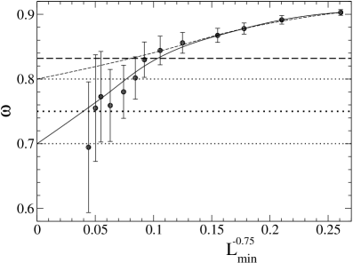
Figure 1: The correction-to-scaling exponent $\omega$, estimated from the fit of $U$ (left) and $U_{6}$ (right) data to the ansatz $A+BL^{-\omega}$ within $L\in[L_{\mathrm{min}},3072]$ and plotted as a function of $L_{\mathrm{min}}^{-0.75}$. The solid and the dashed curves indicate the expected behavior if the asymptotic $\omega$ value is $0.7$ and $0.8$, respectively. These two values correspond to the lower and the upper bound of the MCRG estimate $\omega=0.75(5)$ of [7], noting that $\omega\approx 0.7$ is also the MCRG estimate in [6]. The central values with the error bounds of $\omega=0.75(5)$ are shown by horizontal dotted lines, whereas the horizontal dashed line indicates the MC value $\omega=0.832(6)$ of [2].

We observe that our estimated exponent $\omega$ tends to decrease below the commonly accepted MC value $0.832(6)$ of [2] with increasing of $L_{\mathrm{min}}$. Therefore, we have found it interesting to test the consistency of this behavior with the already mentioned in Sec. 1 MCRG estimates $\omega\approx 0.7$ and $\omega=0.75(5)$ [6, 7]. For this purpose, we have plotted the estimated $\omega$ as a function of $L_{\mathrm{min}}^{-0.75}$, since this plot is expected to be an almost linear function of $L_{\mathrm{min}}^{\omega-\bar{\omega}}\sim L_{\mathrm{min}}^{-0.75}$ at large $L_{\mathrm{min}}$, because the subleading correction term $\mathcal{O}\left(L^{-\bar{\omega}}\right)$ is by a factor $L^{\omega-\bar{\omega}}$ smaller than $L^{-\omega}$. The used here relation $\omega-\bar{\omega}\approx-0.75$ is true if $\bar{\omega}=2\omega$ and $\omega\approx 0.75$ hold. Here we have considered $\bar{\omega}=2\omega$ as a plausible possibility, representing the case when the subleading correction is, in fact, the second-order correction of the type $\left(L^{-\omega}\right)^{2}=L^{-2\omega}$. Another possibility is $\bar{\omega}=\omega_{2}$, if $\omega_{2}<2\omega$, where $\omega_{2}$ is the second irrelevant RG exponent. It is $\omega_{2}=1.67(11)$ according to [19]. Thus, we generally have $\bar{\omega}=\min\{2\omega,\omega_{2}\}$ and $\bar{\omega}-\omega\approx 0.75$ for $\omega\approx 0.75$. Hence, it is meaningful to plot the estimated $\omega$ as a function of $L_{\mathrm{min}}^{-0.75}$ for our testing purposes.

We have drawn in Fig. 1 spline curves, which converge asymptotically almost linearly to certain values, i. e., $\omega=0.7$ (solid curves) and $\omega=0.8$ (dashed curves). The solid curves fit the data very well, thus illustrating a plausible scenario of convergence towards $\omega\approx 0.7$ in a good agreement with the MCRG estimation of [6]. It corresponds also to the lower bound of the MCRG estimate $\omega=0.75(5)$ of [7]. The upper bound of this estimate corresponds to the dashed curves in Fig. 1, which fit the data marginally well. Hence, from a purely statistical point of view, $\omega\approx 0.8$ is also plausible and even $\omega\approx 0.83$ is possible, but, with a larger probability, $\omega<0.8$ holds.

Note that the MC estimation in [2] is also based on the $U$ and $U_{6}$ data at $\beta=\bar{\beta}_{c}$, just as here. The value $\omega=0.832(6)$ of [2] has a relatively small statistical error, however, their estimation is based on $L_{\mathrm{min}}\leq 20$ and $L_{\mathrm{max}}=360$, whereas we have $L_{\mathrm{min}}\leq 64$ and $L_{\mathrm{max}}=3456$. Moreover, the range $L_{\mathrm{min}}\leq 20$ corresponds to just 6 smallest–$L_{\mathrm{min}}$ data points in Fig. 1, from which the deviation of $\omega$ below $0.83$ is still not seen. We do not rule out a possibility that this deviation is caused by statistical errors in the data. On the other hand, such a deviation is more convincingly confirmed by the analysis of the susceptibility data in Sec. 4, and the agreement with the MCRG estimations, perhaps, is also not accidental.

4 The estimation of $\omega$ in the $U=1.6$ scaling regime

Here we consider the scaling regime $\beta=\widetilde{\beta}(L)$, corresponding to $U=\langle m^{4}\rangle/\langle m^{2}\rangle^{2}=1.6$. The precise value of $U$ is not crucial, and one can choose $1<U<3$ for the scaling analysis. Using $U=1.6$ as a near-to-critical value, the correction-to-scaling exponent $\omega$ has been estimated in [4] from the ratios of the susceptibility $\chi(2L)/\chi(L/2)$, which scale as $A+BL^{-\omega}$ at $L\to\infty$. The result, obtained from the $\chi(L)$ data within $L\in[40,2560]$ was $\omega=0.21(29)$. A similar estimation from the refined data in Tab. 2 within $L\in[40,3456]$ gives $\omega=0.67(15)$. Hence, one can conclude that the unusually small value of $\omega$ obtained earlier in [4] is partly due to the large statistical errors. Therefore, the conjecture $\omega\leq\omega_{\mathrm{max}}$ with $\omega_{\mathrm{max}}\approx 0.38$, proposed earlier in [4], probably could not be confirmed. A problem here is that this conjecture is based on a theorem proven in [31], the conditions of which have been numerically verified only in the two-dimensional $\phi^{4}$ model.

For a more accurate estimation, we have evaluated $\omega$ by fitting the susceptibility data to the ansatz

$$\chi(L)=L^{2-\eta}\left(a_{0}+a_{1}L^{-\omega}\right)$$ (2)

with fixed critical exponent $\eta=0.0362978(20)$, provided by the conformal bootstrap method [13]. It is well justified, since our actual estimation of $\eta$ in Sec. 6 perfectly agrees with this $\eta$ value. We have fitted the data within $L\in[L_{\mathrm{min}},3456]$ and have plotted in Fig. 2 the resulting $\omega$ estimates as a function of $L_{\mathrm{min}}^{-0.75}$ in order to compare them with the MCRG values, based on the same arguments as in Sec. 3.

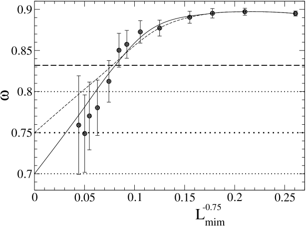
Figure 2: The correction-to-scaling exponent $\omega$, estimated from the fit of the susceptibility data to the ansatz (2) with fixed $\eta=0.0362978(20)$ (taken from [13]) within $L\in[L_{\mathrm{min}},3456]$ and plotted as a function of $L_{\mathrm{min}}^{-0.75}$. The dashed and the solid curves indicate the expected behavior if the asymptotic $\omega$ value is $0.75$ and $0.7$, respectively. These two values correspond to the central value and the lower bound of the MCRG estimate $\omega=0.75(5)$ of [7], noting that $\omega\approx 0.7$ is also the MCRG estimate in [6]. The central values with the error bounds of $\omega=0.75(5)$ are shown by horizontal dotted lines, whereas the horizontal dashed line indicates the MC value $\omega=0.832(6)$ of [2].

According to the solid curve in Fig. 2, the behavior of $\omega$ well agrees with the $\omega\approx 0.7$ estimate in [6], which is also the lower bound of the $\omega=0.75(5)$ estimate in [7]. This behavior is less consistent with the central value $0.75$ of the latter estimation – see the dashed line in Fig. 2, suggesting that this central value could be slightly overestimated rather than underestimated.

Up to now, we have only tested the consistency of $\omega$ vs $L_{\mathrm{min}}$ behavior with the values of MCRG. For an independent estimation, we have fit the $\chi(L)$ data to a refined ansatz

$$\chi(L)=L^{2-\eta}\left(a_{0}+a_{1}L^{-\omega}+a_{2}L^{-\bar{\omega}}\right)\,,$$ (3)

where $\eta=0.0362978(20)$, as before, and $\bar{\omega}$ is also fixed. The meaning of $\bar{\omega}=\min\{2\omega,\omega_{2}\}$ has been already discussed in Sec. 3. The main advantage of (3) in comparison with (2) is that it gives more stable values of $\omega$, which do not essentially change with $L_{\mathrm{min}}$ for $L_{\mathrm{min}}\geq 20$. Moreover, the inclusion of the correction term $a_{2}L^{-\bar{\omega}}$ improves the quality of the fit, reducing the value of $\chi^{2}/\mathrm{d.o.f.}$ of the fit from $1.46$ to $1.24$ at $\bar{\omega}=1.5$ and $L_{\mathrm{min}}=20$. We have set $L_{\mathrm{min}}=20$ as the best choice, since it gives the smallest statistical error among the fits with $L_{\mathrm{min}}\geq 20$. The fitting results are collected in Tab. 3.

Table 3: The values of $\omega$ depending on $\bar{\omega}$, obtained by fitting the susceptibility data to the ansatz (3) within $L\in[20,3456]$ at $\eta=0.0362978(20)$. The $\chi^{2}/\mathrm{d.o.f.}$ of the fit is indicated in the third column.

$\bar{\omega}$	$\omega$	$\chi^{2}/\mathrm{d.o.f.}$
1.7	0.718(56)	1.24
1.6	0.701(61)	1.24
1.5	0.679(68)	1.24
1.4	0.651(76)	1.24

Evidently, the estimated $\omega$ decreases with decreasing of $\bar{\omega}$. Taking into account the statistical error bars of one $\sigma$ and choosing $\bar{\omega}$ self-consistently, i. e., $\bar{\omega}\leq 2\omega$, our fitting procedure suggests that $\omega<0.75$ most probably holds. More precisely, $\omega<0.75$ holds if our fit at the correct value of $\bar{\omega}$ does not underestimate $\omega$ by more than one standard error $\sigma$. Recall that the possibility $\omega<0.75$ is supported also by the behavior seen in Fig. 2.

5 A critical re-examination of MCRG data

For a more complete picture, we have reanalysed the MCRG data of [7], providing some original idea about the estimation of $\omega$ from the MCRG iterations. In [7], one starts with some lattice size $L$ and makes $n$ renormalization iterations. In each iteration, the lattice size shrinks by the factor $b=2$, so that the final lattice size is $L_{f}=2^{-n}L$. Our idea is to look on the MCRG data in a somewhat different way than the authors of [7] originally did. Instead of considering a sequence with fixed $L$ and $n=1,2,\ldots$, we propose to look on a sequence of data with fixed final lattice size $L_{f}$ and $n=1,2,\ldots$ It ensures that the finite-size effects do not increase along such a sequence. We can fit one such sequence to evaluate the considered critical exponent at $n\to\infty$ at a given $L_{f}$. Then we can compare the fit results for sequences with different $L_{f}$, say, $L_{f}=8$ and $L_{f}=16$, to make a finite-size correction on $L_{f}$.

We have applied this method to the estimation of $\omega$, using the $-y_{T2}\equiv\omega$ data in Tab. V of [7] at the maximal number of operators $N_{e}=30$ considered there. Following the idea in [6], we have plotted $\omega$ as a function of $2^{-\omega n}$ in Fig. 3, using here $0.75$ as an approximate self-consistent value of $\omega$. It allows us to estimate the asymptotic $\omega$ at $n\to\infty$ by a linear or a quadratic extrapolation. Apparently, there is some finite-size effect in this estimation, since the linearly extrapolated $\omega$ values (see the solid lines in Fig. 3) slightly depend on $L_{f}$. Namely, we have $\omega=0.7853(48)$ at $L_{f}=8$ and $\omega=0.7672(80)$ at $L_{f}=16$. The finite-size correction is expected to be $\sim L_{f}^{-\omega}$ with $\omega\approx 0.75$. The corresponding linear extrapolation of $\omega(L_{f})$ as a function of $L^{-0.75}$ gives the estimate $\omega=0.741(21)$ for $L_{f}=\infty$. This value is indicated in Fig. 3 by the horizontal dotted line. This estimation perfectly agrees with that in [7], but the statistical error bars are significantly smaller. Thus, one could judge that $\omega$ is, indeed, significantly smaller than $0.83$.

However, there are still uncertainties about the possible systematic errors, as pointed out below.

1. The evaluation in Fig. 3 is based on linear fits (the solid straight-line fits), but the data plots may have some curvature (see the dashed fit curves in Fig. 3). Unfortunately, this curvature cannot be reliably estimated because of too large statistical errors.

2. There is an uncertain systematical error caused by the inaccuracy in the value of the critical coupling $\beta_{c}$, used in the simulations by Ron et. al. [7]. Indeed, the used there value $0.2216544$ is slightly underestimated. A more precise value is $0.22165462$, as it can be seen from Tabs. 1 and 2, as well as from a recent MC estimation in [5].

3. The number of operators has been limited to $N_{e}\leq 30$ in [7], not even including all those ones considered in [6]. A larger number of operators might be important.

These uncertainties should be resolved for a reliable estimation of the critical exponents, including $\omega$.

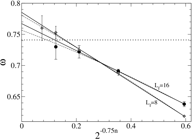
Figure 3: The correction-to-scaling exponent $\omega$ depending on $2^{-0.75n}$ according to the MCRG data in [7], where $n$ is the number of MCRG iterations, starting with the lattice size $L=2^{n}L_{f}$ and ending up with the lattice size $L_{f}$. The data with $L_{f}=8$ and $L_{f}=16$ are shown by diamonds and circles, respectively. The linear (solid lines) and quadratic (dashed lines) fits show the estimated convergence to certain $\omega$ values at $n\to\infty$ for the given $L_{f}$. The horizontal dotted line represents the estimated asymptotic (at $n\to\infty$) value $0.741(21)$ of $\omega$ at $L_{f}=\infty$.

6 Estimation of the critical exponents $\eta$ and $\nu$

We have estimated the critical exponent $\eta$ by fitting the susceptibility data in Tabs. 1 and 2 to the ansatz (2). The fitting results, depending on the minimal lattice size $L_{\mathrm{min}}$ included in the fit, are collected in Tabs. 4 and 5, respectively. In these tables, $\eta_{0}$ is the estimate of $\eta$ without corrections to scaling, obtained by formally setting $a_{1}=0$ in (2). The other two estimates $\eta_{1}$ and $\eta_{2}$ are obtained by fitting the data to the full ansatz (2) with fixed exponent $\omega=0.75$ (for $\eta_{1}$) or $\omega=0.832$ (for $\eta_{2}$). The results for $\beta=\bar{\beta}(L)$ in Tab. 4 appear to be more accurate than those for $\beta=\widetilde{\beta}(L)$ in Tab. 5. Besides, the results without corrections to scaling ($\eta_{0}$) show some trend, therefore the inclusion of the correction term is meaningful. It allows to fit the data reasonably well already starting with $L_{\mathrm{min}}=16$. Moreover, it stabilises the $\eta_{1}$ and $\eta_{2}$ values in such a way that the estimates at $L_{\mathrm{min}}=16$ and $L_{\mathrm{min}}>16$ perfectly match. Since $L_{\mathrm{min}}=16$ ensures the smallest statistical error in this case, our final result ($\eta_{1}$ from Tab. 4) is $\eta=0.03632(13)$. Here we have chosen $\omega=0.75$, as it well coincides with our estimations in Secs. 3 and 4, but $\omega=0.832$ gives practically the same result $\eta=0.03630(12)$ ($\eta_{2}$ from Tab. 4). Note also that the $\eta_{1}$ and $\eta_{2}$ estimates in Tab. 5 perfectly agree with those in Tab. 4, only the statistical error bars are larger.

Table 4: The MC estimates $\eta_{0}$, $\eta_{1}$ and $\eta_{2}$ of the critical exponent $\eta$, obtained by fitting the susceptibility data at $\beta=\bar{\beta}_{c}(L)$ (Tab. 1) within $L\in[L_{\mathrm{min}},3072]$ at different values of $L_{\mathrm{min}}$. The estimates $\eta_{0}$ are provided by the fits without corrections to scaling (setting $a_{1}=0$ in (2)), whereas $\eta_{1}$ and $\eta_{2}$ are obtained by fitting the data to (2) with fixed $\omega=0.75$ and $\omega=0.832$, respectively. The $\chi^{2}/\mathrm{d.o.f.}$ of the fits for $\eta_{0}$, $\eta_{1}$ and $\eta_{2}$ are given in the columns Nr. 3, 5 and 7, respectively.

$L_{\mathrm{min}}$	$\eta_{0}$	​$\chi^{2}/\mathrm{d.o.f}$​	$\eta_{1}$	​$\chi^{2}/\mathrm{d.o.f}$​	$\eta_{2}$	​$\chi^{2}/\mathrm{d.o.f}$​
16	0.037295(66)	3.60	0.03632(13)	1.20	0.03630(12)	1.20
20	0.037062(77)	2.43	0.03625(16)	1.21	0.03622(14)	1.21
24	0.036877(85)	1.56	0.03636(18)	1.20	0.03631(16)	1.20
27	0.036764(94)	1.29	0.03644(20)	1.20	0.03638(17)	1.20
32	0.03670(11)	1.28	0.03642(22)	1.25	0.03637(19)	1.25
40	0.03664(12)	1.28	0.03642(27)	1.30	0.03636(23)	1.31
48	0.03653(14)	1.21	0.03669(31)	1.25	0.03659(27)	1.25

Table 5: The MC estimates $\eta_{0}$, $\eta_{1}$ and $\eta_{2}$ of the critical exponent $\eta$, obtained by fitting the susceptibility data at $\beta=\widetilde{\beta}_{c}(L)$ (Tab. 2) within $L\in[L_{\mathrm{min}},3456]$ at different values of $L_{\mathrm{min}}$. The estimates $\eta_{0}$ are provided by the fits without corrections to scaling (setting $a_{1}=0$ in (2)), whereas $\eta_{1}$ and $\eta_{2}$ are obtained by fitting the data to (2) with fixed $\omega=0.75$ and $\omega=0.832$, respectively. The $\chi^{2}/\mathrm{d.o.f.}$ of the fits for $\eta_{0}$, $\eta_{1}$ and $\eta_{2}$ are given in the columns Nr. 3, 5 and 7, respectively.

$L_{\mathrm{min}}$	$\eta_{0}$	​$\chi^{2}/\mathrm{d.o.f}$​	$\eta_{1}$	​$\chi^{2}/\mathrm{d.o.f}$​	$\eta_{2}$	​$\chi^{2}/\mathrm{d.o.f}$​
16	0.03807(15)	2.93	0.03633(29)	1.32	0.03599(26)	1.31
20	0.03768(17)	2.32	0.03600(35)	1.25	0.03574(30)	1.27
24	0.03737(19)	1.87	0.03595(40)	1.30	0.03570(35)	1.31
27	0.03719(21)	1.77	0.03585(43)	1.34	0.03561(38)	1.35
32	0.03682(23)	1.36	0.03615(48)	1.31	0.03587(42)	1.32
40	0.03655(27)	1.27	0.03646(58)	1.32	0.03615(50)	1.34
48	0.03649(30)	1.31	0.03665(67)	1.37	0.03632(58)	1.38

We have estimated the critical exponent $\nu$ by fitting the $\partial Q/\partial\beta$ data (where $Q=1/U$) at $\beta=\widetilde{\beta}_{c}(L)$ (see Tab. 2) to the ansatz

$$\frac{\partial Q}{\partial\beta}=L^{1/\nu}\left(a_{0}+a_{1}L^{-\omega}\right)$$ (4)

within $L\in[L_{\mathrm{min}},3456]$. The results are collected in Tab. 6. The $\partial Q/\partial\beta$ data at $\beta=\bar{\beta}_{c}(L)$ can also be used, however, these data provide fits of significantly lower quality (with $\chi^{2}/\mathrm{d.o.f.}\gtrsim 1.83$) and somewhat larger statistical errors.

Table 6: The MC estimates $\nu_{0}$, $\nu_{1}$ and $\nu_{2}$ of the critical exponent $\nu$, obtained by fitting the $\partial Q/\partial\beta$ data at $\beta=\widetilde{\beta}_{c}(L)$ (Tab. 2) within $L\in[L_{\mathrm{min}},3456]$ at different values of $L_{\mathrm{min}}$. The estimates $\nu_{0}$ are provided by the fits without corrections to scaling (setting $a_{1}=0$ in (4)), whereas $\nu_{1}$ and $\nu_{2}$ are obtained by fitting the data to (4) with fixed $\omega=0.75$ and $\omega=0.832$, respectively. The $\chi^{2}/\mathrm{d.o.f.}$ of the fits for $\nu_{0}$, $\nu_{1}$ and $\nu_{2}$ are given in the columns Nr. 3, 5 and 7, respectively.

$L_{\mathrm{min}}$	$\nu_{0}$	​$\chi^{2}/\mathrm{d.o.f}$​	$\nu_{1}$	​$\chi^{2}/\mathrm{d.o.f}$​	$\nu_{2}$	​$\chi^{2}/\mathrm{d.o.f}$​
16	0.63048(19)	1.35	0.63026(38)	1.38	0.63028(33)	1.38
20	0.63047(22)	1.40	0.63008(45)	1.41	0.63011(39)	1.41
24	0.63041(25)	1.44	0.62999(52)	1.46	0.63002(45)	1.46
27	0.63046(27)	1.49	0.62969(56)	1.45	0.62975(49)	1.44
32	0.63017(31)	1.38	0.63008(63)	1.44	0.63005(55)	1.43
40	0.62996(36)	1.38	0.63075(75)	1.38	0.63061(65)	1.38
48	0.63011(40)	1.42	0.63080(88)	1.44	0.63067(76)	1.45

The $\nu$ estimates, denoted by $\nu_{0}$ in Tab. 6, are obtained neglecting the correction term $a_{1}L^{-\omega}$ in (4), whereas $\nu_{1}$ and $\nu_{2}$ are the estimates with fixed $\omega=0.75$ and $\omega=0.832$, respectively. In fact, we can see from Tab. 6 that the inclusion of the correction term neither improves the quality of the fits nor remarkably changes the fitting results. Hence, the estimation without corrections to scaling is appropriate in this case. The estimate $\nu=\nu_{0}=0.63048(19)$ at $L_{\mathrm{min}}=16$ has the smallest statistical error and the corresponding fit has the smallest $\chi^{2}/\mathrm{d.o.f.}$ value. On the other hand, this $\nu_{0}$ value is the largest one among those listed in Tab. 6. Therefore, to avoid a possible tiny overestimation because of a too small value of $L_{\mathrm{min}}$, we have assumed $\nu=0.63017(31)$, obtained at $L_{\mathrm{min}}=32$, as our final estimate. This value closely agrees with all other estimates in Tab. 6.

Summarising our MC estimation of the critical exponents $\eta$ and $\nu$, we note that our final estimates $\eta=0.03632(13)$ and $\nu=0.63017(31)$ perfectly agree with the “exact” values of the conformal bootstrap method, i. e., $\eta=0.0362978(20)$ and $\nu=0.6299709(40)$ [13].

7 Discussion and outlook

The critical exponents $\eta=0.03632(13)$ and $\nu=0.63017(31)$ of our MC analysis of very large lattices ($L\leq 3456$) agree well with the known CFT values [13], which are claimed to be extremely accurate or “exact”. It rises the confidence about correctness of our MC simulations and analysis.

Our MC analysis suggests that the correction-to-scaling exponent $\omega$ could be smaller than the commonly accepted value about $0.83$, thus supporting the MCRG estimates $\omega\approx 0.7$ [6] and $\omega=0.75(5)$ [7]. Of course, due to the statistical errors, our fits can appear to be wrong by more than one $\sigma$. In fact, the fit to (3) should be wrong by $\approx 2\sigma$ to reach the consistency with $\omega=0.832(6)$ in [2] or $\omega=0.82951(61)$ in [14]. This is possible, although the agreement with the MCRG estimates allows us to think that the observed deviation of $\omega$ below $0.83$ with increasing of $L_{\mathrm{min}}$ in Figs. 1 and 2 is a real effect. There is still a question whether or not this deviation represents the true asymptotic behavior. Indeed, we cannot exclude a possibility that the estimated $\omega$ values would increase, being accurately extracted from the data for even larger lattice sizes. To test this scenario, accurate enough data for very large lattice sizes should be obtained. It requires an enormous computational effort. Theoretically, the asymptotic $\omega$ value could appear to be larger due to some correction term(s), which are not yet included in (3). For example, $\propto L^{-1}$ correction term in the brackets of (3) could significantly influence the results because the exponent $1$ is close to $0.83$. Unfortunately, we currently do not have any theoretical argument for the existence of such a correction term in the 3D Ising model. One could just try to make fits with extra terms included in (3). From a technical point of view, however, such fits are problematic, as they require higher accuracy of the data.

Taking into account the computational efforts required for the above discussed improved MC analysis, a refining of MCRG estimation, in order to control and eliminate the systematical errors discussed in Sec. 5, is a more feasible task. If $\omega$ is, indeed, about $0.83$, then we should see the convergence of the MCRG iterations to this value. Based on a systematic and rigorous analysis of the MCRG data (as, e. g., proposed in Sec. 5), sufficiently accurate and reliable estimates of $\omega$ could be easily obtained, slightly extending the simulations, e. g., to $L=512$, if necessary.

One could judge that $\omega=0.82951(61)$ holds according to the CFT [12, 14], therefore the considered here significantly smaller $\omega$ values describe, in the best case, a transient behavior. On the other hand, the possibility of $\omega<0.8$ cannot be rigorously excluded because of the following issues.

• The CFT is an asymptotic theory. Hence, it should correctly describe the leading scaling behavior, but not necessarily corrections to scaling. Indeed, the MC analysis in [31] shows the existence of non-integer correction-to-scaling exponents in the scalar 2D $\phi^{4}$ model, which are not expected from the CFT. This idea is supported also by the resummed $\varepsilon$-expansion in [25]. It yields $\omega=1.6\pm 0.2$ for this model, simultaneously providing accurate results for the known critical exponents $\gamma$, $\nu$, $\beta$ and $\eta$ in two dimensions. In the 3D Ising model, the subleading correction-to-scaling exponent $\omega_{2}=1.67(11)$, extracted from the nonperturbative RG analysis in [19], apparently does not coincide with the results of the CFT in [14]. Namely, we find $\omega_{2}=3.8956(43)$ in accordance with $\Delta_{\epsilon^{\prime\prime}}=6.8956(43)$ in [14] and the relation $\Delta_{\epsilon^{\prime\prime}}=3+\omega_{2}$ given in [12]. This might be a serious issue, although it still does not rule out a possibility that the CFT could correctly capture the leading corrections to scaling in the 3D Ising model. One could mention that the estimate $\Delta_{\epsilon^{\prime\prime}}=6.8956(43)$ is not rigorous, but nevertheless is considered as “somewhat accurate” in [14].

• Only a subset of all known estimates of $\omega$ in the 3D Ising model well coincide with $\omega=0.82951(61)$. The purely numerical estimations are usually considered as being most reliable. The MC estimates here and in [2] do not well agree. The high temperature series expansion in [10] gives $\omega=\Delta/\nu=0.825(48)$ and confirms $\omega=0.82951(61)$ within the error bars. On the other hand, a more recent estimation by the large mass expansion in [11] gives $\omega\approx 0.8002$. The error bars are not stated here, but one can judge from the series of estimates of the order $N\in[21,25]$, i. e., 0.92800, 0.86046, 0.82024, 0.80411, 0.80023, that $\omega$, probably, is about $0.80$ and significantly smaller than $0.83$. Among other results, the perturbative RG estimates $\omega=0.782(5)$ [26] (from the expansion at fixed dimension $d=3$) and $\omega=0.82311(50)$ [27] (from the $\varepsilon$-expansion) can be mentioned, as they are claimed to be very accurate. The first one could be less accurate due to the singularity of the Callan-Symanzik $\beta$-function [32]. The estimates from the truncated nonperturbative RG equations are $\omega=0.870(55)$ and $\omega=0.832(14)$, obtained in [17] from the derivative expansion at the $O\left(\partial^{2m}\right)$ order with $m=1$ and $m=2$, respectively. The stated here error bars, however, include only the uncertainty of estimation at the given order. Thus, the expected final result at $m\to\infty$ is still unclear.

In summary, the MC and MCRG data analysed in this paper suggest that the correction-to-scaling exponent $\omega$ of the 3D Ising model could be somewhat smaller than usually expected. However, we do not have enough data to be sure. The precise value of $\omega$ is a quantity which merits a further consideration and testing. In particular, it would be very meaningful to resolve the problems and challenges of the MCRG simulations outlined in this paper. As we believe, it would lead to sufficiently accurate and reliable estimates of $\omega$. In view of the above discussion, it would be also very interesting to evaluate the subleading correction-to-scaling exponent $\omega_{2}$ from the MCRG simulations.

References

- [1] M. Hasenbusch, Int. J. Mod. Phys. C 12, 911 (2001).
- [2] M. Hasenbusch, Phys. Rev. B 82, 174433 (2010).
- [3] I. A. Campbell, P. H. Lundow, Phys. Rev. B 83, 014411 (2011).
- [4] J. Kaupužs, R. V. N. Melnik, J. Rimšāns, Int. J. Mod. Phys. C 28, 1750044 (2017).
- [5] A. M. Ferrenberg, J. Xu, D. P. Landau, Phys. Rev. E 97, 043301 (2018).
- [6] R. Gupta, P. Tamayo, Int. J. Mod. Phys. C 7, pp. 305–319 (1996).
- [7] D. Ron, A. Brandt, R. H. Swendsen, Phys. Rev. E 95, 053305 (2017).
- [8] J. Chung, Y. Kao, Phys. Rev. Res. 3, 023230 (2021).
- [9] A. Wipf, High-Temperature and Low-Temperature Expansions. In: Statistical Approach to Quantum Field Theory. Lecture Notes in Physics, vol. 992, Springer, Cham (2021).
- [10] M. Compostrini, A. Pelisseto, P. Rossi, E. Vicari, Phys. Rev. E 65, 066127 (2002).
- [11] H. Yamada, arXiv:1408.4584 [hep-lat] (2014).
- [12] S. El-Showk, M. F. Paulos, D. Poland, S. Rychkov, D. Simmons-Duffin, A. Vichi, J. Stat. Phys. 157, 869 (2014).
- [13] D. Poland, D. Simmons-Duffin, Nature Physics 12, 535 (2016)
- [14] M. Reehorst, arXiv:2111.12093 [hep-th] (2021)
- [15] C. Bagnuls, C. Bervillier, Phys. Rep. 348, 91 (2001)
- [16] J. Berges, N. Tetradis, C. Wetterich, Phys. Rep. 363, 223 (2002)
- [17] G. De Polsi, I. Balog, M. Tissier, N. Wschebor, Phys. Rev. E. 101, 042113 (2020)
- [18] J. Kaupužs, R. V. N. Melnik, J. Phys. A: Math. Theor. 53, 415002 (2020)
- [19] K. E. Newman, E. K. Riedel, Phys. Rev. B 30, 6615 (1984).
- [20] D. J. Amit, Field Theory, the Renormalization Group, and Critical Phenomena, World Scientific, Singapore, 1984.
- [21] S. K. Ma, Modern Theory of Critical Phenomena, W. A. Benjamin, Inc., New York, 1976.
- [22] J. Zinn-Justin, Quantum Field Theory and Critical Phenomena, Clarendon Press, Oxford, 1996.
- [23] H. Kleinert, V. Schulte-Frohlinde, Critical Properties of Theories, World Scientific, Singapore, 2001.
- [24] A. Pelissetto, E. Vicari, Phys. Rep. 368 (2002) 549–727.
- [25] J. C. Le Guillou, J. Zinn-Justin, J. Physique Lett. 46 (1985) L-137 – L-141.
- [26] A. A. Pogorelov, I. M. Suslov, J. Exp. Theor. Phys. 106, 1118 (2008).
- [27] A. M. Shalaby, Eur. Phys. J. C 81, 87 (2021).
- [28] U. Wolff, Phys. Rev. Lett. 62 (1989) 361.
- [29] J. Kaupužs, J. Rimšāns, R. V. N. Melnik, Phys. Rev. E 81, 026701 (2010).
- [30] E. Bittner, W. Janke, Phys. Rev. E 84, 036701 (2011).
- [31] J. Kaupužs, R. V. N. Melnik, J. Rimšāns, Int. J. Mod. Phys. C 27 (2016) 1650108.
- [32] P. Calabrese, M. Caselle, A. Celi, A. Pelissetto, E. Vicari, J. Phys. A: Math. Gen. 33 (2000) 8155-8170.