Normalized power priors always discount historical data

1 Introduction

Power priors are a class of prior distributions which can be used for incorporation of historical data in Bayesian analysis of current data (Chen and Ibrahim,, 2000). The basic idea is to use the likelihood of the historical data raised to the power of $\alpha$ as the prior distribution for the model parameters $\theta$. This leads to the posterior distribution of $\theta$ borrowing information from both the current and the historical data, typically resulting in an information gain compared to an analysis of the current data in isolation. The power parameter $\alpha$ is usually restricted to the interval between zero and one, thereby determining how much the historical data are discounted and enabling a quantitative compromise between the extreme positions of completely trusting ($\alpha=1$) and completely ignoring them ($\alpha=0$).

In practice, the power parameter $\alpha$ is unknown and therefore often assigned a prior distribution. In this case, the marginal posterior density of the model parameters $\theta$ based on the current data $D$ and the historical data $D_{0}$ is given by

$$\pi(\theta\,|\,D,D_{0})=\int_{0}^{1}\pi(\theta\,|\,D,D_{0},\alpha)\pi(\alpha\,|\,D,D_{0})\text{d}\alpha,$$

that is, the posterior of $\theta$ based on a fixed $\alpha$ averaged over the marginal posterior of $\alpha$. The marginal posterior of $\alpha$ thus determines how much pooling between the two data sets occurs, and a complete pooling of both data sets happens when the posterior has all its mass at $\alpha=1$.

Standard Bayesian asymptotic theory establishes that, under certain regularity conditions, posterior distributions become more concentrated with increasing amounts of data (Bernardo and Smith,, 2000, section 5.3). Since the power prior is based on the historical data, intuition would suggest that as the sample sizes of the current and historical data sets increase, the marginal posterior of $\alpha$ should become increasingly concentrated at $\alpha=0$ if there is conflict between the data sets, and increasingly concentrated at $\alpha=1$ if there is no conflict. Here, we show that only the former is true, but not the latter, at least in the typical situation where $\alpha$ has a beta prior distribution and the data have normal or binomial likelihood. In case of conflict, there is instead a limiting posterior distribution that is hardly different from the prior. Our results imply that complete discounting is possible, but complete pooling is impossible.

This paper is structured as follows: We start by showing the claimed result for parameter estimates under normality (Section 2). We then show that the result also approximately holds in the binomial model (Section 3). The papers then ends with some concluding remarks in Section 4. As a running example we consider data from two randomized clinical trials comparing the efficacy of the drugs Fidaxomicin and Vancomycin on Clostridium difficile-associated diarrhoea in adults (Table 1).

Table 1: Historical and current data on the comparison between Fidaxcomicin and Vancomycin with respect to their effect on Clostridium difficile-associated diarrhoea in adults. The number of participants and events were taken from the respective intention-to-treat analysis of the studies as in the meta-analysis of Nelson et al., (2017).

Study	Risk (Fidaxomicin)	Risk (Vancomycin)	Risk ratio (95% CI)
Cornely et al., (2012)	$\dfrac{193}{270}=71.5\%$	$\dfrac{163}{265}=61.5\%$	$1.16$ (1.04, 1.31)
Louie et al., (2011)	$\dfrac{214}{302}=70.9\%$	$\dfrac{198}{327}=60.6\%$	$1.17$ (1.04, 1.31)

2 Parameter estimates under normality

Define the current data set by $D=\{\hat{\theta},\sigma\}$ with $\hat{\theta}$ an estimate of an unknown univariate parameter $\theta$ and $\sigma$ the (assumed to be known) standard error of the estimate. Denote by $D_{0}=\{\hat{\theta}_{0},\sigma_{0}\}$ the respective quantities obtained from the historical data. The standard errors are usually of the form $\sigma=\kappa/\sqrt{n}$ and $\sigma_{0}=\kappa/\sqrt{n_{o}}$, where $n$ and $n_{0}$ are effective sample sizes and $\kappa^{2}$ is the variance of one unit. The relative variance $c=\sigma^{2}_{0}/\sigma^{2}=n/n_{0}$ can then be interpreted as a ratio of sample sizes. For both estimates, assume a normal likelihood centered around the parameter $\theta$ and with variance equal to the squared standard error. In the default “normalized” version of the power prior (Duan et al.,, 2005; Neuenschwander et al.,, 2009) the prior for the power parameter $\alpha$ is assigned marginally to the posterior distribution of $\theta$ based on an initial prior for $\theta$ and the likelihood of the historical data $D_{0}$ raised to the power of $\alpha$. Here and henceforth we will use an initial uniform prior for the parameter $\pi(\theta)\propto 1$ and a beta prior for the power parameter $\alpha\sim\operatorname{Be}(p,q)$. This choice leads to the normalized power prior

$$\pi(\theta,\alpha\,|\,D_{0})=\frac{L(D_{0}\,|\,\theta)^{\alpha}\pi(\alpha)}{\int_{-\infty}^{+\infty}L(D_{0}\,|\,\theta^{\prime})^{\alpha}\text{d}\theta^{\prime}}=\operatorname{N}(\theta\,|\,\hat{\theta}_{0},\sigma^{2}_{0}/\alpha)\operatorname{Be}(\alpha\,|\,p,q)$$ (1)

with $\operatorname{N}(\cdot\,|\,m,v)$ the normal density function and $\operatorname{Be}(\cdot\,|\,p,q)$ the beta density function. Combining (1) with the likelihood of the current data produces a joint posterior for $\theta$ and $\alpha$, i. e.,

$$\pi(\theta,\alpha\,|\,D,D_{0}) =\frac{L(D\,|\,\theta)\pi(\theta,\alpha\,|\,D_{0})}{\int_{0}^{1}\int_{-\infty}^{\infty}L(D\,|\,\theta^{\prime})\pi(\theta^{\prime},\alpha^{\prime}\,|\,D_{0})\text{d}\theta^{\prime}\text{d}\alpha^{\prime}}=\frac{\operatorname{N}(\hat{\theta}\,|\,\theta,\sigma^{2})\operatorname{N}(\theta\,|\,\hat{\theta}_{0},\sigma^{2}_{0}/\alpha)\operatorname{Be}(\alpha\,|\,p,q)}{\int_{0}^{1}\operatorname{N}(\hat{\theta}\,|\,\hat{\theta}_{0},\sigma^{2}+\sigma^{2}_{0}/\alpha^{\prime})\operatorname{Be}(\alpha^{\prime}\,|\,p,q)\text{d}\alpha^{\prime}},$$

from which a marginal posterior for $\alpha$ can be obtained by integrating out $\theta$, i. e.,

$$\pi(\alpha\,|\,D,D_{0})=\int_{-\infty}^{+\infty}\pi(\theta,\alpha\,|\,D,D_{0})\text{d}\theta=\frac{\operatorname{N}(\hat{\theta}\,|\,\hat{\theta}_{0},\sigma^{2}+\sigma^{2}_{0}/\alpha)\operatorname{Be}(\alpha\,|\,p,q)}{\int_{0}^{1}\operatorname{N}(\hat{\theta}\,|\,\hat{\theta}_{0},\sigma^{2}+\sigma^{2}_{0}/\alpha^{\prime})\operatorname{Be}(\alpha^{\prime}\,|\,p,q)\text{d}\alpha^{\prime}}.$$ (2)

The black solid lines in Figure 1 show the marginal posterior distributions of the power parameter $\alpha$ (left) and the log risk ratio $\theta$ (right) based on a uniform $\alpha\sim\operatorname{Be}(1,1)$ prior for the power parameter and the data from Table 1; the log risk ratio with standard error from the current data $D=\{\hat{\theta}=0.15,\sigma=0.06\}$, and the log risk ratio with standard error from the historical data $D_{0}=\{\hat{\theta}_{0}=0.16,\sigma_{0}=0.06\}$. Both distributions are computed via numerical integration.

The left plot of Figure 1 shows that the observed marginal posterior of $\alpha$ has hardly changed from the uniform prior, despite the almost perfect correspondence of historical and current log risk ratio. The dashed line shows the (soon to be discussed) marginal posterior for the best-case scenario when both log risk ratios perfectly correspond and their standard errors become arbitrarily small. As is visible, this best-case posterior of $\alpha$ is not too far off the observed one, giving only slightly more support to larger values of $\alpha$.

The right plot of Figure 1 shows the corresponding marginal posterior for $\theta$. As can be seen, the observed posterior (solid line) and the best-case posterior (dashed line) are virtually indistinguishable, suggesting that the data achieve as much pooling as the normalized power prior model permits. In contrast, the dotted line indicates that the posterior based on complete pooling of the data sets would be somewhat more peaked.

Figure 1: Power prior modeling of current data $D=\{\hat{\theta}=0.15,\sigma=0.06\}$ from Cornely et al., (2012) and historical data $D_{0}=\{\hat{\theta}_{0}=0.16,\sigma_{0}=0.06\}$ from Louie et al., (2011). A $\alpha\sim\operatorname{Be}(1,1)$ prior is used for the power parameter. Marginal posterior densities are computed by numerical integration.

In general the integral in the denominator of (2) has to be computed by numerical integration, but there are certain important situations when an analytical solution exists, and further insight can be gained. We will discuss these cases in the following.

2.1 Perfect compatibility of historical and current data

The first situation occurs when the current data perfectly mirror the historical data in the sense that both parameter estimates are equivalent ($\hat{\theta}=\hat{\theta}_{0}$). In this case, several terms cancel in (2) so that the integral can be represented in terms of the hypergeometric function ${}_{2}F_{1}(a,b,c;z)=\{\int_{0}^{1}t^{b-1}(1-t)^{c-b-1}(1-tz)^{-a}\text{d}t\}/\mathrm{B}(b,c-b)$ with $\mathrm{B}(x,y)$ the beta function (Abramowitz and Stegun,, 1965, section 15.3.1), i. e.,

$$\pi(\alpha\,|\,D,D_{0},\hat{\theta}=\hat{\theta}_{0}) =\frac{(\alpha/c+1)^{-1/2}\operatorname{Be}(\alpha\,|\,p+1/2,q)}{{}_{2}F_{1}(1/2,p+1/2,p+q+1/2;-1/c)}.$$ (3)

where $c=\sigma^{2}_{0}/\sigma^{2}$ is the relative variance. The distribution (3) is close to a $\operatorname{Be}(p+1/2,q)$ distribution which is hardly different from the $\operatorname{Be}(p,q)$ prior distribution, despite perfect compatibility of both data sets. Importantly, the marginal posterior (3) does not depend on the actual value of the standard errors $\sigma$ and $\sigma_{0}$ but only on the relative variance $c$. This means that (3) holds for finite standard errors but also in the idealized mathematical situation where both standard errors go equally fast to zero (i. e.,  infinite sample size), but with possibly different starting values ($c\neq 1$).

Typically, the historical data are predetermined and only the standard error of the current study can be changed. It is therefore interesting to study the behavior of (3) for $c\to\infty$, i. e.,  the current standard error $\sigma$ goes to zero while the historical standard error $\sigma_{0}$ remains fixed, reflecting an arbitrary increase of the current sample size. In that case it is straightforward to see from the power series representation of the hypergeometric function (Abramowitz and Stegun,, 1965, section 15.1.1) that

$$\lim_{c\to\infty}{}_{2}F_{1}(1/2,p+1/2,p+q+1/2;-1/c) =\lim_{c\to\infty}1+\mathcal{O}(1/c)=1.$$

Hence, the limiting posterior density is

$$\lim_{c\to\infty}\pi(\alpha\,|\,D,D_{0},\hat{\theta}=\hat{\theta}_{0}) =\operatorname{Be}(\alpha\,|\,p+1/2,q),$$ (4)

that is, again a beta density but with updated success parameter $p+1/2$, so just slightly different from the prior. The limiting $\operatorname{Be}(3/2,1)$ distribution for the uniform prior is depicted by the dashed line in the left plot of Figure 1.

2.2 Arbitrarily precise current data

The second situation in which the marginal posterior (2) is available in closed form is the limiting case when the current standard error $\sigma$ goes to zero while the historical standard error $\sigma_{0}$ remains fixed (but in contrast to the previous situation the parameter estimates $\hat{\theta}$ and $\hat{\theta}_{0}$ can take different values). In this case, the integral in (2) can be represented by the confluent hypergeometric function $M(a,b,z)=\{\int_{0}^{1}\exp(zt)t^{a-1}(1-t)^{b-a-1}\text{d}t\}/\mathrm{B}(b-a,a)$ (Abramowitz and Stegun,, 1965, section 13.2.1) so that the marginal posterior is given by

$$\lim_{\sigma\downarrow 0}\pi(\alpha\,|\,D,D_{0}) =\frac{\exp\left\{-\alpha(\hat{\theta}-\hat{\theta}_{0})^{2}/(2\sigma^{2}_{0})\right\}}{M\{p+1/2,p+q+1/2,-(\hat{\theta}-\hat{\theta}_{0})^{2}/(2\sigma^{2}_{0})\}}\operatorname{Be}(\alpha\,|\,p+1/2,q).$$ (5)

As expected, the distribution (5) reduces to (4) when the parameter estimates are equal ($\hat{\theta}=\hat{\theta}_{0}$) since then the left fraction becomes one, which can be shown using the power series representation of the confluent hypergeometric function (Abramowitz and Stegun,, 1965, section 13.1.2).

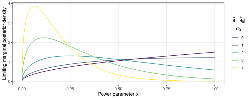
Figure 2: Limiting marginal posterior distribution of power parameter $\alpha$ based on $\alpha\sim\operatorname{Be}(1,1)$ prior and when the current standard error goes to zero ($\sigma\downarrow 0$), for different values of the parameter difference standardized by the historical standard error $|\hat{\theta}-\hat{\theta}_{0}|/\sigma_{0}$.

Figure 2 shows the distribution (5) for different values of the parameter estimate difference standardized by the historical standard error ($|\hat{\theta}-\hat{\theta}_{0}|/\sigma_{0}$). One can see that when the parameter estimates become more different (larger $|\hat{\theta}_{0}-\hat{\theta}|$) the limiting distribution (5) will be increasingly shifted towards smaller values of $\alpha$ indicating more incompatibility among the data sets and reducing the information borrowing from the historical data. This shift amplifies with decreasing historical standard errors $\sigma_{0}$, meaning that the posterior can become arbitrarily peaked by increasing the sample size of the historical study. In contrast, when the parameter estimates are the same ($\hat{\theta}=\hat{\theta}_{0}$) the historical standard error $\sigma_{0}$ does not influence the posterior.

The marginal posterior for $\alpha$ can thus at best become a $\operatorname{Be}(p+1/2,q)$ if the prior is a $\operatorname{Be}(p,q)$, implying that a complete pooling of historical and current data can never be achieved. On the other hand, a complete discounting is possible since conflict between the current and historical data can make the marginal posterior arbitrarily peaked at $\alpha=0$. However, considering that the distribution (5) is based on an extremely informative current data set which lead to an estimate of the unknown parameter $\theta$ without any measurement error, the rate at which the posterior becomes more concentrated seems also dissatisfactory. For instance, for a standardized parameter difference $|\hat{\theta}-\hat{\theta}_{0}|/\sigma_{0}=3$, the posterior is only slightly peaked at around $\alpha=0.1$.

3 Binomial model

So far we assumed a normal likelihood and a univariate parameter, Appendix A shows that the previous result can be generalized to normal linear models with multivariate parameter $\theta$. In this section, we will show that the previous result also holds approximately in the binomial model, which is an important model class in medical applications of power priors.

Let $D=\{x,n\}$ and $D_{0}=\{x_{0},n_{0}\}$ denote the number of successes and total trials from current data and historical data set, respectively. Assume a binomial likelihood with success probability $\theta$ for each of them, and let $\hat{\theta}=x/n$ and $\hat{\theta}_{0}=x_{0}/n_{0}$ denote the respective maximum likelihood estimates. Assigning an initial beta prior $\theta\sim\operatorname{Be}(0,0)$ for the success probability and a beta prior $\alpha\sim\operatorname{Be}(p,q)$ for the power parameter leads to the normalized power prior

$$\pi(\theta,\alpha\,|\,D_{0}) =\operatorname{Be}\{\theta\,|\,\alpha x_{0},\alpha(n_{0}-x_{0})\}\operatorname{Be}(\alpha\,|\,p,q).$$ (6)

Combining the prior (6) with the likelihood of the current data leads to a joint posterior distribution for $\theta$ and $\alpha$, from which a marginal posterior for $\alpha$ can be obtained by integrating out $\theta$, i. e.,

$$\pi(\alpha\,|\,D,D_{0})=\frac{\operatorname{BeBin}\{x\,|\,n,\alpha x_{0},\alpha(n_{0}-x_{0})\}\operatorname{Be}(\alpha\,|\,p,q)}{\int_{0}^{1}\operatorname{BeBin}\{x\,|\,n,\alpha^{\prime}x_{0},\alpha^{\prime}(n_{0}-x_{0})\}\operatorname{Be}(\alpha^{\prime}\,|\,p,q)\text{d}\alpha^{\prime}}$$ (7)

with $\operatorname{BeBin}(\cdot\,|\,n,p,q)$ the beta-binomial probability mass function.

As for the normal model, the integral in the denominator of (7) is generally not available in closed form. Yet again, it is possible to obtain a closed form expression when the probability estimates from both studies are equivalent ($\hat{\theta}=\hat{\theta}_{0}$). Application of Stirling’s approximation $\mathrm{B}(x,y)\approx\sqrt{2\pi}x^{x-1/2}y^{y-1/2}(x+y)^{-(x+y-1/2)}$ to both beta functions in the probability mass function of the beta-binomial leads then to

$$\operatorname{BeBin}\{x\,|\,n,\alpha x_{0},\alpha(n_{0}-x_{0})\} \approx\binom{n}{x}\hat{\theta}^{x}(1-\hat{\theta})^{n-x}\sqrt{\frac{\alpha n_{0}}{n+\alpha n_{0}}}.$$ (8)

Using the approximation (8) in numerator and denominator of (7) produces the same marginal posterior (3) as for the normal model but with $c=n/n_{0}$, representing the relative sample size of the data sets. The limiting marginal posterior distribution of $\alpha$ is thus (approximately) the same for normal and binomial model.

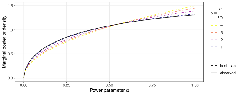
Figure 3: Marginal posterior of power parameter $\alpha$ based on $\alpha\sim\operatorname{Be}(1,1)$ prior and historical data $D_{0}=\{x_{0}=214,n_{0}=302\}$ from Louie et al., (2011). The black solid line shows the marginal posterior for the actually observed current data $D=\{x=193,n=270\}$ from Cornely et al., (2012), whereas the dashed lines show the best-case marginal posteriors for hypothetical current data $D=\{x=c\times x_{0},n=c\times n_{0}\}$ which perfectly mirror the original data but with relative sample sizes $c=n/n_{0}$.

Figure 3 shows the marginal posterior (7) based on the data from Table 1 using the risk in the Fidaxomicin group as the parameter of interest. The black solid line depicts the posterior based on the observed data from Cornely et al., (2012), whereas the dashed lines depict posteriors based on hypothetical data which perfectly mirror the historical data (i. e.,  with identical probability estimates $\hat{\theta}=\hat{\theta}_{0}$) from Louie et al., (2011) but with different relative sample sizes $c=n/n_{0}$. Numerical integration is used for computing the posterior in all finite sample size cases, for $c\to\infty$ the limiting distribution (4) is shown. It can be seen that the limiting posterior density based on Stirling’s approximation (yellow line) is close to the exact posterior for finite relative sample sizes $c$, suggesting that the approximation is reasonably accurate. Moreover, the observed marginal posterior (which has $c=0.89$) is very close to the best-case posterior for $c=1$, indicating that the data achieve almost as much pooling as the power prior permits in that case.

4 Discussion

We showed that normalized power priors in normal and binomial models combined with beta priors assigned to the power parameter $\alpha$ have undesirable and counterintuitive properties. Specifically, in the best-case scenario when the current data perfectly mirror the historical data and the sample sizes from both data sets become arbitrarily large, the marginal posterior of $\alpha$ does not converge to a point mass at $\alpha=1$ but approaches a $\alpha\sim\operatorname{Be}(p+1/2,q)$ distribution, hardly differing from the prior $\alpha\sim\operatorname{Be}(p,q)$. The result implies that a complete pooling of historical and current data can never be achieved. Our case study illustrates that the property is not only a mathematical curiosity but can occur in statistical analysis of medical data.

We still believe that normalized power priors are useful since they permit arbitrarily large data-driven discounting of historical data. However, data analyst should be aware that this does not work in the other direction as the amount of possible pooling is predetermined by the prior. Data analysts have different options to alleviate this limitation. For instance, they can use the power prior based on a fixed $\alpha$ and use either a “guide value” (Ibrahim et al.,, 2015) or elicit a reasonable value from external knowledge about the similarity of the data sets. Another option is to specify informative priors which give most of their mass to larger values of $\alpha$, thereby shifting the best-case marginal posterior to larger values as well. Finally, a pragmatic alternative is to specify $\alpha$ via an empirical Bayes approach as proposed by Gravestock and Held, (2017), which permits complete pooling of both data sets.

We only studied the limiting marginal posterior of $\alpha$ in the normal and binomial models combined with beta priors on $\alpha$, yet we conjecture that the issue is more fundamental and also present in other types of models. However, this will likely be more difficult to establish as marginal posteriors are typically not available in closed form for more complex models.

For the normal model, there is an exact correspondence between power parameter models with fixed $\alpha$ and hierarchical (random-effects meta-analysis) models with fixed heterogeneity variance (Chen and Ibrahim,, 2006). This connection may provide an intuition for why the counterintutive result occurs: Precisely estimating a heterogeneity variance from two observations alone (the historical and current data sets) seems like an impossible task as the “unit of information” is the number of data sets and not the number of samples within a data set. We report elsewhere on the precise connection between power parameter and hierarchical models when power parameter and the heterogeneity variance are random (Pawel et al.,, 2022).

Software and data

The summary data used in this study were extracted from Figure 5.1 in Nelson et al., (2017). All analyses were conducted in the R programming language version 4.3.0 (R Core Team,, 2022). The packages ggplot2 (Wickham,, 2016) and hypergeo (Hankin,, 2016) were used used for graphics and (confluent) hypergeometric function implementation, respectively. The code and data to reproduce our analyses is openly available at https://github.com/SamCH93/ppPooling. A snapshot of the GitHub repository at the time of writing is available at https://doi.org/10.5281/zenodo.6626963.

Appendix A Normal linear model

Define the current data by $D=\{\mathbf{y},\mathbf{X}\}$ with $\mathbf{y}$ an $n\times 1$ vector of observations and $\mathbf{X}$ an $n\times k$ matrix of known covariates. Assume a linear model $\mathbf{y}=\mathbf{X}\boldsymbol{\theta}+\boldsymbol{\varepsilon}$ with $\boldsymbol{\theta}$ a $k\times 1$ vector of parameters and $\boldsymbol{\varepsilon}$ an $n\times 1$ vector of random errors whose components are independently normally distributed around zero with (known) variance $\sigma^{2}$ variance. Denote by $D_{0}=\{\mathbf{y}_{0},\mathbf{X}_{0}\}$ the respective quantities from a historical data set. Finally, let $\hat{\boldsymbol{\theta}}=(\mathbf{X}^{\top}\mathbf{X})^{-1}\mathbf{X}^{\top}\mathbf{y}$ and $\hat{\boldsymbol{\theta}}_{0}=(\mathbf{X}^{\top}_{0}\mathbf{X}_{0})^{-1}\mathbf{X}^{\top}_{0}\mathbf{y}_{0}$ denote the respective maximum likelihood estimates of $\boldsymbol{\theta}$. Based on a uniform initial prior $\pi(\boldsymbol{\theta})\propto 1$ for the parameter vector and a beta prior $\alpha\sim\operatorname{Be}(p,q)$ for the power parameter, we obtain the normalized power prior

$$\pi(\boldsymbol{\theta},\alpha\,|\,D_{0}) =\operatorname{N}_{\text{k}}\left(\boldsymbol{\theta}\,|\,\hat{\boldsymbol{\theta}}_{0},\sigma^{2}\alpha^{-1}(\mathbf{X}^{\top}_{0}\mathbf{X}_{0})^{-1}\right)\operatorname{Be}(\alpha\,|\,p,q)$$ (9)

with $\operatorname{N}_{\text{k}}(\cdot\,|\,\boldsymbol{\mu},\boldsymbol{\Sigma})$ the density function of a $k$-variate normal. Updating the prior (9) with the likelihood of the current data leads to a joint posterior for $\boldsymbol{\theta}$ and $\alpha$, from which a marginal posterior for $\alpha$ can be obtained by integrating out $\boldsymbol{\theta}$, i. e.,

$$\pi(\alpha\,|\,D,D_{0})=\frac{\operatorname{N}_{\text{k}}\left(\hat{\boldsymbol{\theta}}\,|\,\hat{\boldsymbol{\theta}}_{0},\sigma^{2}(\mathbf{X}^{\top}\mathbf{X})^{-1}+\sigma^{2}\alpha^{-1}(\mathbf{X}^{\top}_{0}\mathbf{X}_{0})^{-1}\right)\operatorname{Be}(\alpha\,|\,p,q)}{\int_{0}^{1}\operatorname{N}_{\text{k}}\left(\hat{\boldsymbol{\theta}}\,|\,\hat{\boldsymbol{\theta}}_{0},\sigma^{2}(\mathbf{X}^{\top}\mathbf{X})^{-1}+\sigma^{2}{\alpha^{\prime}}^{-1}(\mathbf{X}^{\top}_{0}\mathbf{X}_{0})^{-1}\right)\operatorname{Be}(\alpha^{\prime}\,|\,p,q)\text{d}\alpha^{\prime}}.$$ (10)

When the current and historical data are perfectly compatible (characterized by equivalent maximum likelihood estimates $\hat{\boldsymbol{\theta}}=\hat{\boldsymbol{\theta}}_{0}$), the integral in (10) can again be represented in terms of the hypergeometric function, and the marginal posterior of $\alpha$ is given by (3) but with $c=|\mathbf{X}^{\top}\mathbf{X}|/|\mathbf{X}^{\top}_{0}\mathbf{X}_{0}|$ the ratio of the determinants of the precision matrices $(\mathbf{X}^{\top}\mathbf{X})/\sigma^{2}$ and $(\mathbf{X}^{\top}_{0}\mathbf{X}_{0})/\sigma^{2}$ of the maximum likelihood estimates $\hat{\boldsymbol{\theta}}$ and $\hat{\boldsymbol{\theta}}_{0}$.

References

- Abramowitz and Stegun, (1965) Abramowitz, M. and Stegun, I. A., editors (1965). Handbook of Mathematical Functions with Formulas, Graphs and Mathematical Tables. Dover Publications, Inc., New York.
- Bernardo and Smith, (2000) Bernardo, J. M. and Smith, A. F. M. (2000). Bayesian Theory. John Wiley & Sons, Chichester, England. doi:10.1002/9780470316870.
- Chen and Ibrahim, (2000) Chen, M.-H. and Ibrahim, J. G. (2000). Power prior distributions for regression models. Statistical Science, 15(1). doi:10.1214/ss/1009212673.
- Chen and Ibrahim, (2006) Chen, M.-H. and Ibrahim, J. G. (2006). The relationship between the power prior and hierarchical models. Bayesian Analysis, 1(3). doi:10.1214/06-ba118.
- Cornely et al., (2012) Cornely, O. A., Crook, D. W., Esposito, R., Poirier, A., Somero, M. S., Weiss, K., Sears, P., and Gorbach, S. (2012). Fidaxomicin versus vancomycin for infection with clostridium difficile in europe, canada, and the USA: a double-blind, non-inferiority, randomised controlled trial. The Lancet Infectious Diseases, 12(4):281–289. doi:10.1016/s1473-3099(11)70374-7.
- Duan et al., (2005) Duan, Y., Ye, K., and Smith, E. P. (2005). Evaluating water quality using power priors to incorporate historical information. Environmetrics, 17(1):95–106. doi:10.1002/env.752.
- Gravestock and Held, (2017) Gravestock, I. and Held, L. (2017). Adaptive power priors with empirical Bayes for clinical trials. Pharmaceutical Statistics, 16(5):349–360. doi:10.1002/pst.1814.
- Hankin, (2016) Hankin, R. K. S. (2016). hypergeo: The Gauss Hypergeometric Function. URL https://CRAN.R-project.org/package=hypergeo. R package version 1.2-13.
- Ibrahim et al., (2015) Ibrahim, J. G., Chen, M.-H., Gwon, Y., and Chen, F. (2015). The power prior: theory and applications. Statistics in Medicine, 34(28):3724–3749. doi:10.1002/sim.6728.
- Louie et al., (2011) Louie, T. J., Miller, M. A., Mullane, K. M., Weiss, K., Lentnek, A., Golan, Y., Gorbach, S., Sears, P., and Shue, Y.-K. (2011). Fidaxomicin versus vancomycin for clostridium difficile nfection. New England Journal of Medicine, 364(5):422–431. doi:10.1056/nejmoa0910812.
- Nelson et al., (2017) Nelson, R. L., Suda, K. J., and Evans, C. T. (2017). Antibiotic treatment for clostridium difficile-associated diarrhoea in adults. Cochrane Database of Systematic Reviews, 3(CD004610). doi:10.1002/14651858.cd004610.pub5.
- Neuenschwander et al., (2009) Neuenschwander, B., Branson, M., and Spiegelhalter, D. J. (2009). A note on the power prior. Statistics in Medicine, 28(28):3562–3566. doi:10.1002/sim.3722.
- Pawel et al., (2022) Pawel, S., Aust, F., Held, L., and Wagenmakers, E.-J. (2022). Power priors for replication studies. doi:10.48550/ARXIV.2207.14720. arXiv preprint.
- R Core Team, (2022) R Core Team (2022). R: A Language and Environment for Statistical Computing. R Foundation for Statistical Computing, Vienna, Austria. URL https://www.R-project.org/.
- Wickham, (2016) Wickham, H. (2016). ggplot2: Elegant Graphics for Data Analysis. Springer International Publishing, Cham, Switzerland. doi:10.1007/978-3-319-24277-4.