Tidal insights into rocky and icy bodies:
An introduction and overview  
 

Abstract

Solid body tides provide key information on the interior structure, evolution, and origin of the planetary bodies. Our Solar system harbours a very diverse population of planetary bodies, including those composed of rock, ice, gas, or a mixture of all. While a rich arsenal of geophysical methods has been developed over several years to infer knowledge about the interior of the Earth, the inventory of tools to investigate the interiors of other Solar-system bodies remains limited. With seismic data only available for the Earth, the Moon, and Mars, geodetic measurements, including the observation of the tidal response, have become especially valuable and therefore, has played an important role in understanding the interior and history of several Solar system bodies. To use tidal response measurements as a means to obtain constraints on the interior structure of planetary bodies, appropriate understanding of the viscoelastic reaction of the materials from which the planets are formed is needed. Here, we review the fundamental aspects of the tidal modeling and the information on the present-day interior properties and evolution of several planets and moons based on studying their tidal response. We begin with an outline of the theory of viscoelasticity and tidal response. Next, we proceed by discussing the information on the tidal response and the inferred structure of Mercury, Venus, Mars and its moons, the Moon, and the largest satellites of giant planets, obtained from the analysis of the data that has been provided by space missions. We also summarise the upcoming possibilities offered by the currently planned missions.

Keywords

Tides, viscoelasticity, Rheology, Mercury, Venus, Moon, Mars, Icy worlds, Interior structure, Surface geology

1 Introduction

The Solar system harbours a diverse population of planetary bodies. These include objects formed of rock, ice, gas, as well as objects of a mixed composition. Over the past two decades, our understanding of these bodies’ interior structure has been considerably improved owing to the valuable data provided by several successful space missions. A combined perception of celestial bodies’ interiors and the mechanisms that govern their evolution can represent an efficient means to infer information about their past history and origins which help us to understand how the Solar system has formed and evolved. Given the scarcity of seismic data for the planetary bodies except the Earth, the Moon, and Mars, our studies have to rely on remote sensing and geodetic measurements. An efficient means to infer knowledge on the planets’ and moons’ interior structure is their tidal response to the gravitational attraction from other objects.

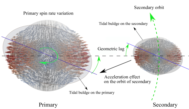
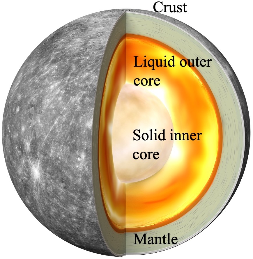
A planet’s side facing its satellite is attracted by the satellite stronger than the opposite side. Since the planet’s rotation is, generally, not synchronised with the period of the orbiting satellite, the satellite exerts a periodically changing force field and a resulting deformation field in the hosting planet. These changes in the gravitational potential generated by the satellite are known as tides (Figure 1). Aside from the well-known ocean tides on the Earth, both the Earth and other planets demonstrate atmospheric tides and, most importantly, bodily tides, a phenomenon on which this review concentrates. This phenomenon is always reciprocal; so the satellite, in its turn, is experiencing periodic perturbation of the planet-generated potential, and is developing periodic deformation. The Sun can also play the same role and generate tides in the planets and itself experiences tides generated by them.

Tidal deformation of a celestial body results in both vertical and horizontal displacement of its surface and in the ensuing perturbation of its gravitational field. These variations are described by three Love numbers: $h$, $l$, and $k$. The two former Love numbers ($h$, $l$) represent the deformations caused by the tidal force on the planet in the vertical and horizontal directions, respectively, whereas $k$ represents the induced perturbation in the gravitational field.

The interior of a planetary body is not perfectly elastic and is affected by internal friction, as a result of which the tidal bulge does not exactly align with the position of the tide-raising body, but exhibits a phase lag. The quality factor $Q$ is defined as the inverse of the sine of the absolute value of the phase angle between the tidal bulge and the direction towards the tide-raising body. It relates to the energy dissipated by friction per loading cycle, in such a way that a lower $Q$ implies higher dissipation. Both the tidal deformation magnitude and the phase lag are sensitive to the large-scale interior properties of the body, such that a larger deformation (higher Love numbers) would imply that the interior of the object is less rigid (contains fluid parts, highly porous material, etc.), while a larger phase lag would imply that the interior is composed of a material that is more viscous. Thus, the tidal response, represented in the form of the tidal Love numbers and tidal quality factor, was used to probe the structural properties of the planetary body. Owing to their long-wavelength nature, tides sample the large-scale interior properties of the body and can be used to probe its deep interior.

Figure 1: Tidal force field and the geometric lag induced in a planet and its satellite resulting from the gravitational attraction of the two bodies towards each another. Tension in the body is shown with red and compression with blue arrows where the size of the arrows indicate the force magnitude. The force field is shown on the unperturbed bodies. The maximum tidal force in the perturbed body is induced in the side of the body that faces the perturber. The tidal evolution changes the orbit period of the satellite and spin rate of the rotation of two bodies, driving their orbital properties towards synchronism.

Studying the planetary tidal response dates backs to Love (1911), in the early 20th century, when the response of a compressible and homogeneous Earth model was first computed. With the increasing precision of modern geodesy, the tidal response of the Earth can be measured by satellite altimetry and the Global Positioning Systems (Yuan et al., 2013); the semi-diurnal tidal Love numbers and the tidal quality factor of the Earth are $k_{2}=0.3531$, $h_{2}=0.6072$, $l_{2}=0.0843$, and $Q\sim 10$, respectively (Seitz et al., 2012; Krásná et al., 2013) (For earlier measurement and analysis, one can refer to Dehant (1987); Mitrovica et al. (1994); Smith et al. (1973); Ryan et al. (1986); Haas and Schuh (1996); Petrov (2000)). Tidal dissipation in the Earth takes place predominantly in the oceans, especially in shallow seas. The dissipation in the oceans excluded, the solid-Earth tidal quality factor is found to be $Q\sim 280\pm 70$ (Egbert and Ray, 2003). Based on such measurements, tidal tomography studies have been efficiently used to constrain the large-scale features of the Earth’s deep interior, such as the nature of two large low-shear-velocity provinces (LLSVP) (Métivier and Conrad, 2008; Latychev et al., 2009; Lau et al., 2017).

The purpose of this review is to provide an introduction to the existing knowledge on the interior of the planetary bodies based on studying their tidal activity. In this review, we cover the fundamental aspects and formulation of the tidal modeling and discuss the role played by tides in understanding the planetary bodies. First, we review the general aspects of viscoelasticity followed by several viscoelastic models used to mimic dissipation in materials, next we provide the fundamental information for modeling the tidal response of a planetary body followed by a brief introduction to tidal evolution and thermal coupling. Next, we discuss the constraints obtained by using the tidal response measurements in understanding the interior properties and evolution of several rocky and icy planetary bodies in the Solar system, i.e., Mercury, Venus, the Moon, Mars, and the largest moons of gas giants. We also discuss what can be learned from measuring the tidal response in the anticipated missions for the planetary bodies which currently lack such data, either completely or with sufficient precision. While this review mostly discusses the interior structure based on measurements of tidal response presented by tidal Love number and tidal quality factor, we also provide a short summary of the surface geological features as a result of tidal activity and its interpretations for the interior properties and evolution of the planetary bodies.

2 Viscoelasticity

Tidal dissipation differs from seismic dissipation, because it is defined not only by the dissipative properties of the mantle but also by the interplay of these properties with the body’s self-gravitation. Leaving the description of this interplay for Section 4, in the current section, we address the rheological properties of the materials, from which the planetary bodies are formed.

2.1 General aspects

Dissipation in a material is, essentially, a relaxation process whose effectiveness is sensitive to the material composition, temperature, confining pressure, grain size and, importantly, to the frequency of forcing. The combined influence of these parameters on the energy damping rate is highly non-trivial, and is defined by complex micro-scale processes such as grain-boundary interactions, dislocation migration and the presence of voids and melt (e.g., Jackson et al., 2002; Jackson and Faul, 2010; McCarthy et al., 2011; Sundberg and Cooper, 2010; Takei et al., 2014). Hence, an appropriate modeling of the viscoelastic behaviour of a celestial body is crucial for the correct interpretation of its tidal measurements.

Mars, as an example, appears to be an instructive case of necessity for such modeling. Compared to the solid-Earth quality factor at semi-diurnal tides ($Q=280\pm 70$, Ray et al. (2001)), the Martian quality factor at the period of Phobos’s tides (T = 5.55 hr) is surprisingly low, i.e., $Q\approx 78-100$, (e.g., Jacobson and Lainey, 2014). Applying the simplistic Maxwell rheology to Mars results in a low quality factor implying an unreasonably low average viscosity ($\sim 10^{14}$ Pa.s) (Bills et al., 2005), in contrast to that estimated for the Earth’s mantle ($\sim 10^{22-23}$ Pa.s) (Anderson and O’Connell, 1967; Karato and Wu, 1993). This result is surprising, given that Mars is expected to have cooled faster on account of its smaller size, and therefore has a higher viscosity value than the solid Earth (See, e.g. Plesa et al. (2018); Khan et al. (2018)). The issue is resolved by employing a more realistic viscoelastic model attributing the high tidal dissipation to strong anelastic relaxation in Mars (Castillo-Rogez and Banerdt, 2012; Nimmo and Faul, 2013; Khan et al., 2018; Bagheri et al., 2019).

Another example revealing the necessity for accurate rheological modeling is Venus. Application of a simplistic elastic model to the mantle would yield to an enticing but naive interpretation for the measured tidal Love number value (Dumoulin et al., 2017; Konopliv and Yoder, 1996). This interpretation would suggest a fully liquid core (Konopliv and Yoder, 1996). However, a fully solid iron core has been shown to be a plausible option, as well, when viscoelasticity is taken into account (Dumoulin et al., 2017; Yoder, 1995). Further insights about tides on Mars and Venus are provided in sections 5.4 and 5.2, respectively. These examples reveal that accurate modeling of viscoelastic dissipation in planetary bodies is essential to understanding their interior structure.

Based on various friction mechanisms involved, several viscoelastic models have been proposed and constrained by means of laboratory experiments (e.g., Gribb and Cooper, 1998; Faul et al., 2004; Jackson, 2005; Jackson and Faul, 2010; Takei et al., 2014). Most of the experimental studies have focused on rocky materials such as olivine and orthopyroxene (see, e.g. Tongzhang Qu and Jackson (2019) and Jackson and Faul (2010)) whereas few studies have considered the dissipation in ice (McCarthy and Cooper, 2016). These models have been utilized to study the planetary data (Lau and Faul, 2019; Nimmo et al., 2012; Nimmo and Faul, 2013; Khan et al., 2018). Because of its ease of implementation, the Maxwell rheology has long been employed to model the viscoelastic behaviour of the planets and moons, and has been especially popular in the studies of very long time-scales such as glacial isostatic adjustment (Al-Attar and Tromp, 2013; Crawford et al., 2018; Ivins et al., 2021; Lau et al., 2021). This model, however, fails to accommodate the transient anelastic behaviour between the fully elastic and viscous regimes (Rambaux et al., 2010; Renaud and Henning, 2018; Castillo-Rogez and Banerdt, 2012), which makes this model inappropriate at seismic and oftentimes at tidal frequencies.

Due to the shortcomings of the Maxwell model , in the later studies, it was suggested to rely on the combined Maxwell-Andrade model, often referred to as simply the Andrade model (e.g., Andrade, 1910; Rambaux et al., 2010; Castillo-Rogez et al., 2011; Efroimsky, 2012). More sophisticated options, such as the Burgers model and the Sundberg-Cooper that incorporate anelasticity as a result of elastically-accommodated and dislocation- and diffusion-assisted grain boundary sliding processes (Burgers, 1935; Sundberg and Cooper, 2010; Jackson, 2005, 2000; Jackson and Faul, 2010). These models are corrected to take into account the effect of grain size, frequency, temperature, and pressure on the dissipation - a fundamental set of parameters that are needed to describe planetary interiors (e.g., Jackson and Faul, 2010).

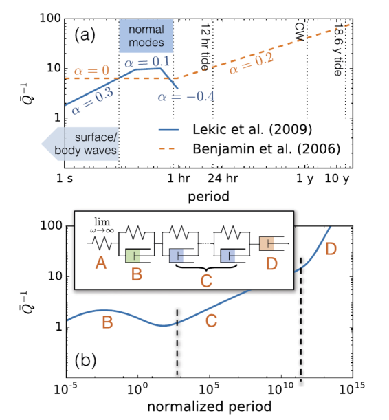
Geophysical analysis enables us to test the viscoelastic models against the attenuation data gleaned over a broad frequency range: from seismic wave periods ($\leq$1 s) over normal modes ($\sim$1 hr), bodily tides (hrs-days), and Chandler Wobble (months), to very long-period tides ($\sim$20 years). This frequency gamut is spanning five orders. Equipped with this knowledge, we can then model the quality factors of planets and use the available measurements to predict the dissipation behaviour over a large range of periods. Figure 2 shows the measured quality factor of the solid Earth as a function of period, ranging from seconds to years, based on the extended Burgers viscoelastic model (described in Section 2.4) constrained by geophysical observations (Lau and Faul, 2019). In this figure, dissipation in the measured surface waves, normal modes, semi-diurnal M2 tides, Chandler Wobble, and the 18.6 yr long-period tides are taken into account. As shown in the figure, studying the dissipation in the Earth, particularly its frequency dependence, has resulted in diverse interpretation, revealing the complexity of this process and the need for further considerations.

Studying the tides is not limited to the rocky planets. In the recent years, substantial attention has been devoted to the tidal dynamics of the icy systems such as Trans-Neptunian Objects, including both the Pluto-Charon binary and Kuiper belt objects (e.g., Bierson et al., 2020; Bagheri et al., 2022; Rhoden et al., 2020; Saxena et al., 2018; Arakawa et al., 2021; Renaud et al., 2021), and the Galilean moons, Iapetus and Enceladus (e.g., Kamata and Nimmo, 2017; Shoji et al., 2014; Spencer, 2013; Tyler, 2009, 2014; Beuthe, 2019; Tyler, 2011). All these bodies are either presently tidally active or experienced significant tidal activity in their history. Understanding the tidal response of these bodies is essential to constrain their origin and in some cases, more importantly, to assess the potential habitability of their interior. Modeling their evolution in their past history requires information on dissipation in ice. Due to the much lower viscosity of ice in comparison to rocks (McCarthy and Cooper, 2016), dissipation in ice can easily dominate that in the rock in the bodies containing both fractions. This applies also to binaries in the outer Solar system where the temperature is too low for the rocky fraction to dissipate energy, and most of the tidal dissipation is taking place in the ice layers. The viscoelastic behaviour of ice is studied using the same models as those used for rocks (Renaud et al., 2021; Sundberg and Cooper, 2010; Bagheri et al., 2022).

The mentioned viscoelastic models have been used to study dissipation in the planetary bodies (discussed in Section 5), although the measurements in the case of other planetary bodies than the Earth are considerably more limited. In the next sections, we review the theoretical aspects of material viscoelastic properties followed by a summary of several laboratory-based rheological models. Note that here we are mostly focusing on the solid body tides, not on the dissipation in fluid parts, such as in the molten core or in the surface or subsurface oceans. The effect of liquid parts is a complex process believed to be responsible for phenomena such as libration of Mercury (e.g., Rambaux et al., 2007; Margot et al., 2007; Peale, 2005) or precession of the Moon (e.g., Yoder, 1981; Cébron et al., 2019; Williams et al., 2001). Moreover, it has been argued that in some circumstances dissipation in the ocean can dominate that in the solid parts (Tyler, 2008; Tyler et al., 2015; Tyler, 2009). However, detailed discussion on the possibility of significant tidal dissipation in the ocean is not in the scope of this study .

Figure 2: (a) The frequency dependence of normalised attenuation, ${\bar{Q}}^{-1}$ for the solid Earth, displaying the contrasting absorption bands of Benjamin et al. (2006) and Lekić et al. (2009) (orange–dashed and blue–solid lines, respectively). The former study used geodetic observations of the semi-diurnal and long period tides, and the Chandler Wobble (CW), whose periods are indicated by the vertical black dotted lines. The latter study used surface wave and normal mode data whose frequency bands are marked by blue boxes. (b) Main panel: schematic frequency dependence of attenuation of the Extended Burgers model (Faul and Jackson, 2015). Inset: the mechanical components of the Extended Burgers model in spring-dashpot representation. Figure and caption modified from Lau and Faul (2019).

2.2 Constitutive equation

Rheological properties of a material are expressed by a constitutive equation linking the present-time deviatoric strain tensor $\,u_{\gamma\nu}(t)\,$ with the values assumed by the deviatoric stress $\,{\sigma}_{\gamma\nu}(t\,^{\prime})\,$ over the time $\,t\,^{\prime}\,\leq\,t\,$. When the rheological response is linear, i.e. when the resulting strain is linear in stress (which is usually the case for strains not exceeding $10^{-6}$ (Karato, 2008) ), the equation is a convolution, in the time domain:

$$2\,u_{\gamma\nu}(t)\,=\,\int^{t}_{-\infty}\stackrel{{\scriptstyle\;\centerdot}}{{J}}(t-t\,^{\prime})~{}{\sigma}_{\gamma\nu}(t\,^{\prime})\,dt\,^{\prime}~{}~{},~{}~{}~{}$$ (1)

and is a product, in the frequency domain:

$$2\;\bar{u}_{\gamma\nu}(\chi)\,=\;\bar{J}(\chi)\;\bar{\sigma}_{\gamma\nu}(\chi)\;\;.$$ (2)

In equation (1), the kernel $\stackrel{{\scriptstyle\;\centerdot}}{{J}}(t-t\,^{\prime})$ is a time derivative of the compliance function ${J}(t-t\,^{\prime})$, also called creep function, which carries all information about the (linear) rheological behaviour of the material.

In equation (2), $\chi$ stands for the frequency, $\,\bar{u}_{\gamma\nu}(\chi)\,$ and $\,\bar{\sigma}_{\gamma\nu}(\chi)\,$ denote the Fourier images of the strain and stress tensors, while the complex compliance function, or simply complex compliance $\,\bar{J}(\chi)\,$ is a Fourier image of $\,{J}(t-t\,^{\prime})\,$. For details, see, e.g. Efroimsky (2012).

While elasticity is a result of bond-stretching along crystallographic planes in an ordered solid, viscosity and dissipation inside a polycrystalline material occur by motion of point, linear, and planar defects, facilitated by diffusion. Each of these mechanisms contributes to viscoelastic behaviour (e.g., Karato, 2008). Deformation of a viscoelastic solid depends on the time evolution of the applied load (Chawla and Meyers, 1999). For small deformations, the stress-strain relation is linear, and the response is described, in the time-domain, by the creep function $J(t)$. Its time derivative links the material properties and forcing stress (the input) with the resulting strain magnitude and phase lag (the output), see equation (1). The response of the material to forcing comprises  (a) an instantaneous elastic response,  (b) a semi-recoverable transient flow regime where the strain rate changes with time, and (c) a steady-state creep. Accordingly, the creep function for a viscoelastic solid consists of three terms:

$$\underbrace{J(t)}_{\text{Creep function}}=\underbrace{J}_{\text{Elastic}}+\underbrace{f(t)}_{\text{Transient strain-rate}}+\underbrace{{t}{/}{\eta}}_{\text{Viscous}},$$ (3)

$t$ and $\eta$ being time and the shear viscosity. The Fourier image of $J(t)$ is the complex compliance $\bar{J}(\chi)=\Re[\bar{J}(\chi)]+i\Im[\bar{J}(\chi)]$, where $\chi$ is the frequency. The associated shear quality factor is given by

$${Q_{s}(\chi)}^{-1}\,=\,\frac{|\,\Im[\bar{J}(\chi)]\,|}{\,\sqrt{\Re^{\textstyle{{}^{2}}}[\bar{J}(\chi)]+\Im^{\textstyle{{}^{2}}}[\bar{J}(\chi)]}}\;\,.$$ (4a)

For solids far from the melting point, the instantaneous (elastic) part of deformation is usually sufficiently large: $$\;|\nobreak\hskip 1.1pt\nobreak\Re[\bar{J}(\chi)]\nobreak\hskip 1.1pt\nobreak|\gg|\nobreak\hskip 1.1pt\nobreak\Im[\bar{J}(\chi)]\nobreak\hskip 1.1pt\nobreak|\,$$, in which case we have

$${Q_{s}(\chi)}^{-1}\,\approx\,\frac{|\,\Im[\bar{J}(\chi)]\,|}{\Re[\bar{J}(\chi)]}\;\,.$$ (4b)

This quality factor is responsible for attenuation of seismic waves, and varies over depth and over geological basins.  An intrinsic material property, $Q_{s}(\chi)$ is different from the degree-$l$ tidal quality factors $Q_{l}(\chi)$ characterising the planet as a whole. As explained in Efroimsky (2012, 2015) and Lau et al. (2017), the distinction comes from the fact that the tidal factors are defined by interplay of self-gravitation with the overall rheological behaviour (generally, heterogeneous). In simple words, self-gravitation pulls the tidal bulge down, thus acting as an effective addition to rigidity. While at sufficiently high frequencies this effect is negligible, it becomes noticeable at the lowest frequencies available to analysis.

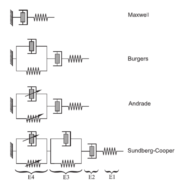
Below, we consider the Maxwell, extended Burgers, Andrade, Sundberg-Cooper rheologies, as well as a simplified power-law scheme. These models were derived from laboratory studies of various regimes of viscoelastic and anelastic relaxation. The applicability realm of each model depends on such parameters as the grain size, temperature, and pressure. Each model can be represented as an arrangement of springs and dashpots connected in series, or in parallel, or in a combination of both connection methods as shown in Figure 3. (Findley and Onaran, 1965; Moczo and Kristek, 2005; Nowick and Berry, 1972; Cooper, 2002; Jackson et al., 2007; McCarthy and Castillo-Rogez, 2013). Instantaneous elastic response is mimicked by a spring, while a fully viscous behaviour is modeled with a dashpot. A series connection (a Maxwell module) implies a non-recoverable displacement, while a parallel connection (a Voigt module) ensures a fully recoverable deformation. Schematic diagrams of four viscoelastic models are shown in Figure (3).

Figure 3:  Schematic representation of viscoelastic models in terms of springs and dashpots. A spring element (E1) represents a purely elastic response, while a dashpot element (E2) is representative of purely viscous damping. A series connection of elements 1 and 2 is representative of the response of a Maxwell model (irrecoverable), while a connection of elements 1 and 2 in parallel (element 3) results in an anelastic (recoverable) response with a discrete (single) spectrum of relaxation times. Arrows on spring and dashpot in element 4, conversely, indicate an element that incorporates a continuous distribution of anelastic relaxation times and results in a broadened response spectrum (Bagheri et al., 2019).

2.3 Maxwell

Maxwell is the simplest model of the viscoelastic behaviour and can be interpreted as a series connection of a spring and dashpot. In the time domain, the creep function for this model is:

$$J(t)=J+\frac{t}{\eta}\,\;,$$ (5)

$\eta$ being the viscosity, and $J$ being the shear elastic compliance related to the shear elastic modulus $\mu$ by

$$J\,=\,\frac{1}{\mu}\;\,.$$ (6)

The real and imaginary parts of the complex compliance are

$$\Re[\bar{J}(\chi)] = J\;\,,$$ (7)

$$\Im[\bar{J}(\chi)] = -\,\frac{1}{\chi\,\eta}\,=\,-\,J\,\frac{1}{\chi\,\tau_{M}}\;\,,$$ (8)

where $\chi$ is the frequency, and the Maxwell time is introduced as

$$\tau_{M}\,=\,\eta\nobreak\hskip 1.1pt\nobreak J\,=\,\frac{\eta}{\mu}~{}~{}.$$ (9)

It is the timescale of relaxation of strain after the stress is abruptly turned off.

Lacking a transient term, the Maxwell model implies an elastic regime at high frequencies and a viscous-fluid regime in the low-frequency limit. It provides a reasonable approximation for reaction to very-long-period loading such as glacial isostatic adjustments (Peltier, 1974). On the other hand, the model is less adequate at tidal and especially seismic frequencies where transient processes are present.

2.4 Burgers and Extended Burgers

The shortcoming of Maxwell’s model in representing a transient response at the frequencies residing between the elastic and viscous bands can be rectified by introducing a time-dependent anelastic transition between these two regimes. This gives birth to the Burgers rheology:

$$J(t)\nobreak\hskip 1.1pt\nobreak=\nobreak\hskip 1.1pt\nobreak J_{U}\nobreak\hskip 1.1pt\nobreak\left[\,1\,+\,\Delta\nobreak\hskip 1.1pt\nobreak\left[1\nobreak\hskip 1.1pt\nobreak-\nobreak\hskip 1.1pt\nobreak\exp\left(\,-\;\frac{t}{\tau}\right)\right]\,+\,\frac{t}{\tau_{M}}\,\right]\;\,,$$ (10)

where $J_{U}$ is the elastic compliance, $\Delta$ is the so-called anelastic relaxation strength, and $\tau$ is a characteristic time of the development of anelastic response. While the Maxwell model does not discriminate between the unrelaxed and relaxed values of $J$, the Burgers model does. From the above expression for $J(t)$, we observe that while $J_{U}$ is the unrelaxed value, $J_{U}\nobreak\hskip 1.1pt\nobreak(1+\Delta)=J_{R}$ is its relaxed counterpart. This conclusion can be deduced also from the expression for the compliance in the complex domain:

$$\bar{J}(\chi)\nobreak\hskip 1.1pt\nobreak=\nobreak\hskip 1.1pt\nobreak\Re\left[\bar{J}(\chi)\right]\,+\,i\,\Im\left[\bar{J}(\chi)\right]\;\;,$$ (11)

$$\Re[\bar{J}(\chi)]\nobreak\hskip 1.1pt\nobreak=\nobreak\hskip 1.1pt\nobreak J_{U}\left(1\nobreak\hskip 1.1pt\nobreak+\nobreak\hskip 1.1pt\nobreak\frac{\Delta}{1\nobreak\hskip 1.1pt\nobreak+\nobreak\hskip 1.1pt\nobreak\chi^{2}\nobreak\hskip 1.1pt\nobreak\tau^{2}}\nobreak\hskip 1.1pt\nobreak\right)~{}~{}~{},\qquad\Im[\bar{J}(\chi)]\;=\;J_{U}\,\Delta\;\frac{\chi\nobreak\hskip 1.1pt\nobreak\tau}{1\nobreak\hskip 1.1pt\nobreak+\nobreak\hskip 1.1pt\nobreak\chi^{2}\nobreak\hskip 1.1pt\nobreak\tau^{2}}~{}~{}~{}.$$ (12)

By inserting these expressions for $\Re[\bar{J}(\chi)]$ and $\Im[\bar{J}(\chi)]$ into definition (4a) for $\nobreak\hskip 1.1pt\nobreak Q^{-1}_{s}\nobreak\hskip 1.1pt\nobreak$,  it is easy to demonstrate that for this model the inverse quality factor possesses a peak, which makes the model applicable to realistic situations where such a peak appears in experiments.

More generally, the anelastic relaxation time $\tau$ can be replaced with a distribution $D(\tau)$ of relaxation times over an interval specified by an upper ($\tau_{H}$) and lower ($\tau_{L}$) bounds (Jackson and Faul, 2010). From a micromechanical point of view, this distribution is associated with diffusionally accommodated grain-boundary sliding. This is how the so-called extended Burgers model emerges:

$$J(t)=J_{U}\left[1+\Delta\int_{\tau_{L}}^{\tau_{H}}D(\tau)\left[1-\exp\left(-\;\frac{t}{\tau}\right)\right]d\tau+\frac{t}{\tau_{M}}\right]\,\;,$$ (13)

where $J_{U}\Delta$, as in the Burgers model, is the increase in compliance associated with complete anelastic relaxation.

The corresponding components of the complex compliance are:

$$\Re[\bar{J}(\chi)] = J_{U}\bigg{(}1+\Delta\int_{\tau_{L}}^{\tau_{H}}\frac{D(\tau)}{1+\chi^{2}\tau^{2}}\;d\tau\bigg{)}\,\;,$$ (14)

$$\Im[\bar{J}(\chi)] = -\,J_{U}\bigg{(}\chi\;\Delta\int_{\tau_{L}}^{\tau_{H}}\frac{\tau D(\tau)}{1+\chi^{2}\tau^{2}}\;d\tau\,+\,\frac{1}{\chi\nobreak\hskip 1.1pt\nobreak\tau_{M}}\bigg{)}\,\;.$$ (15)

A commonly used distribution of anelastic relaxation times associated with the background dissipation is the absorption band model proposed by Minster and Anderson (1981). Within that model, $D(\tau)$ is implemented by the function $D(\tau,\,\alpha)$ bearing a dependence on a fractional parameter $\alpha\,$:

$$D_{B}(\tau,\,\alpha)\;=\;\left\{\begin{array}[]{ll}0&\mbox{for}\;\;\tau\notin[\tau_{L}\,,\;\tau_{H}]\,\;,\\ \frac{\textstyle\alpha\tau^{\alpha-1}}{\textstyle{{\tau_{H}}^{\alpha}-{\tau_{L}}^{\alpha}}}&\mbox{for}\;\;\tau_{L}<\tau<\tau_{H}\,\;,\end{array}\right.$$ (18)

where $0<\alpha<1\,$, while $\tau_{L}$ and $\tau_{H}$ denote the cut-offs of the absorption band where dissipation is frequency-dependent and scales, approximately,   as $Q_{s}\propto\chi^{\alpha}$. The lower bound of the absorption band ensures a finite shear modulus at high frequencies and restricts attenuation at those periods.

Jackson and Faul (2010) found that their experimental data were better fit by including a dissipation peak in the distribution of anelastic relaxation times, which is superimposed upon the monotonic background along with the associated dispersion. This background peak is attributed mostly to sliding with elastic accommodation of grain-boundary incompatibilities (see Takei et al., 2014, for a different view). In this case, $D(\tau)$ writes as

$$D_{P}(\tau)=\frac{1}{\sigma\tau\sqrt{2\pi}}\exp\bigg{(}\frac{-\ln{({\tau}/{\tau_{P}})}}{2\,\sigma^{2}}\bigg{)}$$ (19)

peaked around some $\tau_{P}\nobreak\hskip 1.1pt\nobreak$, a new timescale to be a part of the model.

2.5 Andrade

While the extended Burgers model incorporates a distribution of relaxation times within a restricted time-scale to account for the transient anelastic relaxation, the Andrade model implies a distribution of relaxation times over the entire time domain:

$$J(t)=J_{U}+\beta\nobreak\hskip 1.1pt\nobreak t^{\alpha}+\frac{t}{\eta}\,\;,$$ (20)

where $\alpha$ defines the frequency-dependence of the compliance,   while $\beta$ is qualitatively playing the same role as $\Delta$ in the extended Burgers model (and may, in principle, change with frequency). Having fractional dimensions, the parameter $\beta$ is somewhat unphysical. For this reason, it was suggested by Efroimsky (2012, 2015) to cast the compliance as

$$J(t)=J_{U}\,\left[1\,+\,\left(\frac{t}{\tau_{A}}\right)^{\alpha}+\frac{t}{\tau_{M}}\right]\,\;,$$ (21)

with the parameter $\tau_{A}$ defined through

$$\beta\,=\,\tau_{A}^{-\alpha}\;J_{U}$$ (22)

and named the Andrade time. A justification for this reformulation will be provided shortly.

With $\Gamma$ denoting the Gamma function, the complex compliance corresponding to (21) writes as:

$$\bar{J}(\chi)\,=\,J_{U}\,\left[1\,+\,(i\chi\tau_{A})^{-\alpha}\,\Gamma(1+\alpha)\,-\,i(\chi\tau_{M})^{-1}\right]\,\;,$$ (23)

its real and imaginary parts being

$$\Re[\bar{J}(\chi)]=J_{U}\nobreak\hskip 1.1pt\nobreak\bigg{[}1+\Gamma(1+\alpha)\;(\chi\tau_{A})^{-\alpha}\,\cos\left(\frac{\alpha\pi}{2}\right)\bigg{]}\,\;,$$ (24)

$$\Im[\bar{J}(\chi)]=\,-\,J_{U}\nobreak\hskip 1.1pt\nobreak\bigg{[}\Gamma(1+\alpha)\;(\chi\tau_{A})^{-\alpha}\,\sin\left(\frac{\alpha\pi}{2}\right)\,+\,(\chi\tau_{M})^{-1}\bigg{]}\,\;.$$ (25)

The absorption band in this model extends from 0 to $\infty$. In other words, anelastic relaxation effectively contributes across the entire frequency range from short-period seismic waves to geological time-scales. This generates two problems.

First, in the situations where the anelastic behaviour is dominated by defect unjamming, it has a low-frequency cut-off, as explained by Karato and Spetzler (1990, eqn 17).  The presence of this feature can be built into the Andrade model “by hand,” by assuming that the Andrade time quickly grows to infinity (or, equivalently, that the parameter $\beta$ quickly reduces to zero) as the frequency goes below some threshold value. So, for frequencies below this threshold, the response of the material is overwhelmingly viscoelastic, while above the threshold the response becomes predominantly anelastic. At this point, we can appreciate the convenience of employing $\tau_{A}$ instead of $\beta\,$: it turns out (Castillo-Rogez et al., 2011, Fig 4) that for olivines $\tau_{A}$ and $\tau_{M}$ are similar over an appreciable band of frequencies:

$$\tau_{A}\approx\tau_{M}\,\;.$$ (26)

Second, within the Andrade model it is impossible, by distinction from the Burgers and extended Burgers models, to write down the relaxed value of $J$. This problem finds its resolution within the Sundberg-Cooper and extended Sundberg-Cooper models discussed below.

2.6 Sundberg-Cooper

Similarly to the Maxwell model, in the Andrade model it is conventional to identify the elastic compliance $J$ with its unrelaxed value $J_{U}$. Consequently, just as the Maxwell model is extended to Burgers, so the Andrade model can be extended to that of Sundberg and Cooper (2010), to account for the combined effects of diffusional background and elastically-accommodated grain-boundary sliding:

$$J(t)=J_{U}+J_{U}\Delta\,\left(1-e^{-\;{t}/{\tau}}\right)+\beta\,t^{\alpha}+\frac{t}{\eta}\;\;.$$ (27a)

In terms of the Maxwell and Andrade times, this creep function can be written down as

$$J(t)=J_{U}\nobreak\hskip 1.1pt\nobreak\left[\,1\,+\,\Delta\,\left(1-e^{-\;{t}/{\tau}}\right)+\left(\frac{t}{\tau_{A}}\right)^{\alpha}+\frac{t}{\tau_{M}}\,\right]\;\,.$$ (27b)

In the frequency domain, this compliance becomes

$$\Re[\bar{J}(\chi)]=J_{U}\nobreak\hskip 1.1pt\nobreak\bigg{[}\nobreak\hskip 1.1pt\nobreak 1\,+\,\Gamma(1+\alpha)\;\left(\chi\nobreak\hskip 1.1pt\nobreak\tau_{A}\right)^{-\alpha}\cos\left(\frac{\alpha\pi}{2}\right)\,+\,\frac{\Delta}{1+\chi^{2}\tau^{2}}\,\bigg{]}\,\;,$$ (28)

$$\Im[\bar{J}(\chi)]=\,-\,J_{U}\nobreak\hskip 1.1pt\nobreak\bigg{[}\nobreak\hskip 1.1pt\nobreak\Gamma(1+\alpha)\,(\chi\nobreak\hskip 1.1pt\nobreak\tau_{A})^{-\alpha}\sin\left(\frac{\alpha\pi}{2}\right)\nobreak\hskip 1.1pt\nobreak+\nobreak\hskip 1.1pt\nobreak\chi\;\frac{\tau\,\Delta}{1+\chi^{2}\tau^{2}}\;\,+\,\left(\chi\nobreak\hskip 1.1pt\nobreak\tau_{M}\right)^{-1}\nobreak\hskip 1.1pt\nobreak\bigg{]}\,\;,$$ (29)

the corresponding $Q_{s}^{-1}(\chi)$ possessing a peak.

A further extension of the Sundberg-Cooper model can be performed in analogy with the extended Burgers model. The term containing the parameter $\tau$ can be replaced with an integral specifying a distribution of anelastic relaxation times $\tau$, as in equation (13).

The real and imaginary parts of the complex compliance for the extended Sundberg-Cooper model are:

$$\Re[\bar{J}(\chi)]=J_{U}\nobreak\hskip 1.1pt\nobreak\bigg{[}\nobreak\hskip 1.1pt\nobreak 1\,+\,\Gamma(1+\alpha)\;\left(\chi\nobreak\hskip 1.1pt\nobreak\tau_{A}\right)^{-\alpha}\cos\left(\frac{\alpha\pi}{2}\right)\,+\,\Delta\int_{\tau_{L}}^{\tau_{H}}\frac{D(\tau)}{1+\chi^{2}\tau^{2}}\;d\tau\,\bigg{]}\,\;,$$ (30)

$$\Im[\bar{J}(\chi)]=\,-\,J_{U}\nobreak\hskip 1.1pt\nobreak\bigg{[}\nobreak\hskip 1.1pt\nobreak\Gamma(1+\alpha)\,(\chi\nobreak\hskip 1.1pt\nobreak\tau_{A})^{-\alpha}\sin\left(\frac{\alpha\pi}{2}\right)\nobreak\hskip 1.1pt\nobreak+\nobreak\hskip 1.1pt\nobreak\chi\;\Delta\int_{\tau_{L}}^{\tau_{H}}\frac{\tau\,D(\tau)}{1+\chi^{2}\tau^{2}}\;d\tau\,+\,\left(\chi\nobreak\hskip 1.1pt\nobreak\tau_{M}\right)^{-1}\nobreak\hskip 1.1pt\nobreak\bigg{]}\,\;,$$ (31)

where $D(\tau)$ is given either by expression (19) or by (18). In the latter case, it is important to mind the difference between the Andrade exponential $\alpha$ and the parameter entering distribution (18). While in equation (18) we denoted the parameter with the same letter $\alpha$ and wrote the function as $D_{B}(\tau,\,\alpha)$, in equations (30 - 31) this function should appear as $D_{B}(\tau,\,\alpha_{1})$, with $\alpha_{1}$ generally different from the Andrade $\alpha$.

2.7 Power-law Approximation

Finally, we consider a power-law approximation sometimes used for fitting measurements (e.g., Jackson et al., 2002). As we shall now demonstrate, this description follows from the Andrade model (24 - 25) under the simplifying assumptions that the anelastic dissipation is weak and that the viscoelastic dissipation is even weaker:

$$\mbox{Assumption~{}\,1}\nobreak\hskip 1.1pt\nobreak: \quad(\chi\nobreak\hskip 1.1pt\nobreak\tau_{A})^{-\alpha}\nobreak\hskip 1.1pt\nobreak\ll\,1\,\;,$$ (32a)

$$\mbox{Assumption~{}\,2}\nobreak\hskip 1.1pt\nobreak: \quad(\chi\nobreak\hskip 1.1pt\nobreak\tau_{M})^{-1}\,\ll\,(\chi\nobreak\hskip 1.1pt\nobreak\tau_{A})^{-\alpha}\,\;.\qquad\qquad$$ (32b)

Approximations (4b) and (32b) enable us to write the inverse shear quality factor as

$$Q_{s}^{-1}\,\equiv\;\frac{|\,\Im[\bar{J}(\chi)]\,|}{|\bar{J}(\chi)|}\;\approx\;\frac{J_{U}}{|\bar{J}(\chi)|}\;\Gamma(1+\alpha)\;(\chi\nobreak\hskip 1.1pt\nobreak\tau_{A})^{-\alpha}\;\sin\left(\frac{\alpha\nobreak\hskip 1.1pt\nobreak\pi}{2}\right)\,\;.$$ (33)

Equivalently,

$$Q_{s}^{-1}\,\cot\left(\frac{\alpha\nobreak\hskip 1.1pt\nobreak\pi}{2}\right)\approx\;\frac{J_{U}}{|\bar{J}(\chi)|}\;\Gamma(1+\alpha)\;(\chi\nobreak\hskip 1.1pt\nobreak\tau_{A})^{-\alpha}\;\cos\left(\frac{\alpha\nobreak\hskip 1.1pt\nobreak\pi}{2}\right)\,\;,$$ (34)

With aid of inequalities (32), $|\bar{J}(\chi)|$ can be written down as

$$|\bar{J}(\chi)|\;\approx\;J_{U}\nobreak\hskip 1.1pt\nobreak\left[1\nobreak\hskip 1.1pt\nobreak+\nobreak\hskip 1.1pt\nobreak\Gamma(1+\alpha)\,(\chi\nobreak\hskip 1.1pt\nobreak\tau_{A})^{-\alpha}\,\cos\left(\frac{\alpha\nobreak\hskip 1.1pt\nobreak\pi}{2}\right)\nobreak\hskip 1.1pt\nobreak\right]~{}~{}.$$ (35)

Combining equations (34) and (35), we arrive at

$$\frac{J_{U}}{|\bar{J}(\chi)|}\;\approx\;1\;-\;Q_{s}^{-1}\,\cot\left(\frac{\alpha\nobreak\hskip 1.1pt\nobreak\pi}{2}\right)\,\;.$$ (36)

Also, the approximate expression (33) can be concisely reparameterised through the forcing period $2\pi/\chi\,$:

$$Q_{s}^{-1}\nobreak\hskip 1.1pt\nobreak\approx\,A\,\left(\frac{2\nobreak\hskip 1.1pt\nobreak\pi}{\chi}\right)^{\alpha}~{}~{}~{},\qquad A\nobreak\hskip 1.1pt\nobreak=\nobreak\hskip 1.1pt\nobreak\Gamma(1+\alpha)\,\sin\left(\frac{\alpha\pi}{2}\right)\,(2\pi\tau)^{-\alpha}~{}~{}~{}.$$ (37)

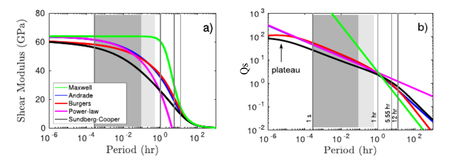
Together, equations (36 - 37) constitute a simplified version of the Andrade model, a version that is valid when both assumptions (32) are fulfilled, which is often the case at seismic frequencies. Figure 4 compares the frequency-dependent shear modulus and the quality factors rendered by different rheological models (Bagheri et al., 2019). This figure readily reveals that Maxwell model and power-law fail to provide appropriate results in a wide range of periods. The other three models, i.e. the extended Burgers, Andrade, and Sundberg-Cooper ones, sometimes render similar dependencies, though in Section 5 we shall see that the choice of the right rheology may become very important in modeling of tides.

Figure 4: Computed variations of relaxed shear modulus ($G_{R}$) and shear attenuation ($Q_{s}$) with period for the five rheological models considered in this study. (a, b) ($G_{R}$) and ($Q_{s}$) as a function of period at constant temperature and grain size; the vertical lines show periods of interest: seismic body waves (1 s), normal modes (1 hr), main tidal excitation of Phobos on Mars (5.55 hr), and main tidal excitation of the Sun (12.32 hr). Figure is modified from Bagheri et al. (2019)

2.8 Rescaling for different values of the temperature, pressure, and grain size

To make a rheological model practical, it is necessary to endow the timescales and other parameters of the model with a dependency on the grain size $d$, temperature $T$, and pressure $P$. For the Maxwell time, Morris and Jackson (2009); Jackson and Faul (2010); McCarthy et al. (2011) suggested the following rescaling prescription:

$$\tau_{M}(T,P,d)=\tau_{M0}\bigg{(}\frac{d_{g}}{d_{0}}\bigg{)}^{m_{gv}}\exp\bigg{[}\bigg{(}\frac{E^{*}}{R}\bigg{)}\bigg{(}\frac{1}{T}-\frac{1}{T_{0}}\bigg{)}\bigg{]}\exp\bigg{[}\bigg{(}\frac{V^{*}}{R}\bigg{)}\bigg{(}\frac{P}{T}-\frac{P_{0}}{T_{0}}\bigg{)}\bigg{]},$$ (38)

where $R$ is the gas constant, $E^{*}$ is the activation energy, $V^{*}$ is the activation volume, $m_{gv}$ is the grain size exponent for viscous relaxation, $P$ is the pressure, $T$ is the temperature, and $\tau_{M0}$ is a normalised value of the Maxwell time at a particular set of reference conditions ($d_{0}$, $P_{0}$, and $T_{0}$). In this expression, both exponential functions come from the rescaling of viscosity $\eta$, under the assumption that the rigidity $\mu$ stays unchanged under the variations of both $T$ and $P$. This assumption is acceptable for temperatures not exceeding about 3/4 of the melting temperature, which in its turn, is a function of pressure.

While the above formula is sufficient to rescale the Maxwell model, it is more complicated in the case of the Burgers model with its additional timescale $\tau$, and even more involved for the extended Burgers model with its three additional timescales $\tau_{L}$, $\tau_{H}$, $\tau_{P}$. Jackson and Faul (2010) suggested to extend (38) to all these timescales:

$$\tau_{i}(T,P,d)=\tau_{i0}\bigg{(}\frac{d_{g}}{d_{0}}\bigg{)}^{m_{g}}\exp\bigg{[}\bigg{(}\frac{E^{*}}{R}\bigg{)}\bigg{(}\frac{1}{T}-\frac{1}{T_{0}}\bigg{)}\bigg{]}\exp\bigg{[}\bigg{(}\frac{V^{*}}{R}\bigg{)}\bigg{(}\frac{P}{T}-\frac{P_{0}}{T_{0}}\bigg{)}\bigg{]},$$ (39)

where all parameters are as in equation (38), while $i=M,\nobreak\hskip 1.1pt\nobreak L,\nobreak\hskip 1.1pt\nobreak H,\nobreak\hskip 1.1pt\nobreak P$. The grain size exponential $m_{g}$ can be different for the anelastic ($m_{ga}$ for $i=L,H,P$) and viscous ($m_{gv}$ for $i=M$) relaxation regimes.

In the case of the Andrade model, Jackson and Faul (2010) adjust for the variations of $d$, $T$, and $P$ by replacing the actual period with the following pseudo-period:

$$X=\chi^{-1}\bigg{(}\frac{d_{g}}{d_{0}}\bigg{)}^{-m_{g}}\exp\bigg{[}\bigg{(}\frac{-E^{*}}{R}\bigg{)}\bigg{(}\frac{1}{T}-\frac{1}{T_{0}}\bigg{)}\bigg{]}\exp\bigg{[}\bigg{(}\frac{-V^{*}}{R}\bigg{)}\bigg{(}\frac{P}{T}-\frac{P_{0}}{T_{0}}\bigg{)}\bigg{]}\,\;.$$ (40)

This is equivalent to a simultaneous rescaling of both the Maxwell and Andrade times by formula (38). To apply it to the Andrade time, one may hypothesise that $\tau_{A}$ and $\tau_{M}$ either are equal or are staying proportional within the considered realm of temperatures, pressures and grain sizes. For $\tau_{A}$, the power $m_{g}$ should assume its anelastic value $m_{ga}$, like in the case of the Burgers model. While this rescaling is natural for the Maxwell time, its applicability to the Andrade time still requires justification.

Similarly to the complete Andrade model, its simplified version (36 - 37) becomes subject to prescription (40). In equation (37), a replacement of the actual forcing period $2\pi/\chi$ with the pseudo-period $X$ given by equation (40) yields:

$$Q_{s}^{-1}\approx A\nobreak\hskip 1.1pt\nobreak X^{\alpha}\;\,.$$ (41)

Just as in the case of the full Andrade model, the applicability of this rule to the power law needs further study.

The parameters involved in the viscoelastic models often need to be better constrained. Extensive experimental work has been carried out in this direction. (Jackson, 2000, 2005; Jackson and Faul, 2010; Jackson et al., 2007, 2002; Sundberg and Cooper, 2010; Tongzhang Qu and Jackson, 2019; McCarthy et al., 2011)  In addition, understanding of the effects of porosity or the presence of partial melt needs further research. Constraints on the effect of the involved parameters will help to obtain more detailed insights into the interiors of the planetary bodies and to develop interpretation of the existing and upcoming measurements. In the literature on tides, each of the afore-mentioned viscoelastic models has been used. In Sections 3 and 4, we address other aspects required for modeling the tidal response of planetary bodies. Those aspects are used in combination with the viscoelastic models to constrain interior properties of the planets and moons, as discussed in Section 5.

3 Tidal and thermal evolution in planetary systems

3.1 Tidal evolution

Viscoelastic tidal dissipation in gravitationally interacting planetary bodies results in an angular momentum exchange between the spin and orbit of the bodies. This process results in an evolution of the spin and orbital rates towards low spin-orbit resonances, e.g. 1:1 for most moons or 3:2 for Mercury, and damping of the eccentricity and inclination of the orbit. The conservation of the angular momentum of the two-body system implies an evolution of the separation, eccentricity, and inclination, while the dissipation of the rotational kinetic energy leads to heat deposition in the orbital partners. When the perturbed body rotates faster than the perturber is orbiting above its surface, the tidal bulge leads the perturber and exerts such a torque on the perturber that the semimajor axis of the orbit expands. On the other hand, if the tidally perturbed body rotates slower than the perturber’s orbital rate, the bulge lags behind and exerts on the perturber a torque contracting the semimajor axis, provided the orbital eccentricity is not very large. The boundary between these cases is commonly defined by a distance between the two bodies, known as synchronous radius, at which the perturber’s mean motion equals the hosting body’s spin rate. This popular belief, however, was shown by Bagheri et al. (2021) to be only applicable for the low-eccentricity orbits, i.e., in the case of highly eccentric orbits, even a satellite above the synchronous radius can migrate towards its hosting planet.

Studying of the orbital evolution of celestial bodies helps to constrain the history of the planetary systems and their origin. For example, numerous studies have targeted the dynamical evolution of the Earth-Moon system, exploiting the Moon’s present-day separation rate of $38.08\pm 0.19$ mm/yr observed from Lunar Laser Ranging (LLR), employing various tidal evolution models (Webb, 1982; Touma and Wisdom, 1998; Williams et al., 2014; Rufu and Canup, 2020; Wisdom and Tian, 2015; Ćuk et al., 2016; Canup and Asphaug, 2001; Zahnle et al., 2015). The discovery of the unexpectedly rapid migration of the Saturnian moon Titan ($\sim 11$ cm/yr) (Lainey et al., 2020) has been used to explain the large obliquity of Saturn. This measurement invalidates the traditional belief (Hamilton and Ward, 2004) that the presently observed obliquity of the rotation axis of Saturn is a result of the crossing of a resonance between the its spin-axis precession and the nodal orbital precession mode of Neptun that has happened during the late planetary migration more than 4 Gyrs ago. Instead, Saillenfest et al. (2021) proposed that the resonance was encountered more recently, about 1 Gyr ago, and forced Saturn’s obliquity to increase from a small value to its current state. Another example is the measurement of the Martian moon, Phobos’s migration rate towards its host at a rate of $\sim 1.8$ cm/yr. This observation has been used to constrain the Martian moons’ origin and interior properties (Yoder, 1982; Bagheri et al., 2021; Singer, 1968; Samuel et al., 2019) as discussed in Section 5.4. Based on this observation, it has been also shown that Phobos will collide with Mars’s surface in $\sim$30-50 Myrs (e.g., Bills et al., 2005).

The rate at which tidal evolution takes place depends on the orbital parameters such as the distance between the two bodies, spin and orbital periods, eccentricity of the orbit, and on the physical properties of these bodies’ interiors, that affect viscoelastic dissipation. Modeling tidal evolution comprises the following major steps:

(1)  Decomposition of the tidal potential into Fourier harmonic modes.

(2)  Assigning to each Fourier mode a specific phase delay and magnitude decrease.

The first step can be carried out by means of a development by Kaula (1964) who explicitly wrote down Fourier expansions for both the perturbing potential and the additional tidal potential of the perturbed body. To perform the second step, simplified tidal models such as constant phase lag model (CPL) (MacDonald, 1964; Goldreich, 1966; Murray and Dermott, 1999) and constant time lag model (CTL) (Singer, 1968; Mignard, 1979, 1980, 1981; Hut, 1981; Heller et al., 2011) were introduced for analytical treatment and applied to rocky moons and planets, as well as gas giants.

Despite the common use of the CTL and CPL models, they have been shown to suffer problems of both physical and mathematical nature (Efroimsky and Makarov, 2013, 2014); The CTL model implies that all the tidal strain modes experience the same temporal delay relative to the corresponding stress modes (Efroimsky and Makarov, 2013; Makarov and Efroimsky, 2013). The CPL model, on the other hand, is not supported by physical principles because it assumes a constant tidal response independent of the excitation frequency which is incompatible with geophysical and laboratory data as shown in various studies (Jackson and Faul, 2010; Jackson, 2005; Khan et al., 2018; Bagheri et al., 2019; Lau and Faul, 2019; Nimmo et al., 2012; Nimmo and Faul, 2013). These shortcomings of the CTL and CPL models are resolved by assigning separate phase lag and amplitude decrease to each Fourier mode. This assignment is defined by the rheology of the body and is also influenced by its self-gravitation. A combination of the properly performed steps (1) and (2) provides a means for calculating spin-orbit evolution of planets and moons (Boué and Efroimsky, 2019), including modeling their capture into spin-orbit resonances (Noyelles et al., 2014). Further extensions to the formulation presented by Boué and Efroimsky (2019) were developed to incorporate highly eccentric orbits and included the effect of dissipation as a result of libration in longitude (Bagheri et al., 2021; Renaud et al., 2021; Bagheri et al., 2022).

3.2 Tidal-thermal evolution coupling

Tidal dissipation is not only responsible for the observed orbits and spin states of celestial bodies, but also can affect these bodies’ thermal evolution. Thermal evolution is responsible for the planetary bodies’ differentiation, melting, and volcanism. The principal heat sources in a binary system are (see e.g., Hussmann et al. (2006)):  (a) the heating associated with accretion during planet formation, (b) the gravitational energy released during planetary differentiation, (c) radiogenic heating in the silicate component due to the decay of long-lived radioactive isotopes (U, Th, and K), and (d) tidal heating due to viscoelastic dissipation. Of these sources, only (c) and (d) are of relevance for the long-term evolution of the planet while the two first sources are mostly linked to the early stages of planetary accretion.

Thermal evolution implies heat being transported to the surface of the body either by conduction or convection, and as a consequence, the interior temperature varies with time. This results in substantial changes in the interior structure and physical properties of the body, such as viscosity and rigidity, which in turn, can considerably change the tidal response of the body and affect its orbital evolution and spin. In the solar system, we can find several examples where tidal and thermal evolution affect one another. For example, in Europa, tidal heating can be intense enough to maintain the presence of a liquid surface or subsurface ocean, though there is no consensus on whether the tidal dissipation is taking place predominantly in the ocean or the ice shell (e.g., Tyler et al., 2015; Choblet et al., 2017; Hussmann and Spohn, 2004; Tobie et al., 2003; Rhoden and Walker, 2022; Sotin et al., 2009). Moreover, tidal heating can result in volcanism, like in Io, considerably exceeding the heating by long-term radiogenic isotopes (e.g., Peale et al., 1979; Van Hoolst et al., 2020; Kervazo et al., 2022; Foley et al., 2020; de Kleer et al., 2019a, b). When considerable portion of ice or liquid water is present inside the body, tidal heating can entail cryovolcanism. This is believed to be the case in several icy moons such as Enceladus, Titan, Europa, and Triton (e.g., Spencer et al., 2009; Sohl et al., 2014; Vilella et al., 2020; Hansen et al., 2021; Hay et al., 2020). In all of the mentioned examples, the tidal and thermal evolution have co-modulating effects on each other. This, necessitating their joint consideration in evaluating the evolution and present-day state of planetary systems. Since in this paper we mostly focus on tides with referring to thermal evolution only in cases where tidal dissipation plays an important role, we do not provide more details on thermal evolution modeling.

4 Tidal potential, Love numbers, and tidal response

4.1 Static tides

Consider a spherical body of radius $\nobreak\hskip 1.1pt\nobreak R\nobreak\hskip 1.1pt\nobreak$. An external perturber of mass $\nobreak\hskip 1.1pt\nobreak M^{\,*}\nobreak\hskip 1.1pt\nobreak$, located at a point $\,{\mbox{{\boldmath$r$}}}^{\;*}=(r^{*},\,\lambda^{*},\,\phi^{*})\,$, in the body frame, generates the following disturbing potential at a point $\,\mbox{{\boldmath${R}$}}=(R,\phi,\lambda)\,$ on the surface of the body:

$$W(\mbox{{\boldmath${R}$}}\,,\,\mbox{{\boldmath$r$}}^{~{}*})~{}=~{}\sum_{n=2}^{\infty}~{}W_{n}(\mbox{{\boldmath${R}$}}\,,~{}\mbox{{\boldmath$r$}}^{~{}*})~{}=~{}-~{}\frac{G\;M^{*}}{r^{\,*}}~{}\sum_{{\it{n}}=2}^{\infty}\,\left(\,\frac{R}{r^{~{}*}}\,\right)^{\textstyle{{}^{\it{n}}}}\,P_{\it{n}}(\cos\gamma)~{}~{},$$ (42)

where $\nobreak\hskip 1.1pt\nobreak R\,<\,r^{*}\,$, the letter $\nobreak\hskip 1.1pt\nobreak G$ denotes the Newton gravity constant, $\phi$ is the latitude reckoned from the spherical body’s equator, $\lambda$ is the longitude reckoned from a fixed meridian, $P_{n}(\cos\gamma)$ are the Legendre polynomials, while $\gamma$ is the angular separation between the vectors $\,{\mbox{{\boldmath$r$}}}^{\;*}\,$ and  ${R}$  pointing from the center of the perturbed body.

In a static picture, the additional tidal potential arising from the deformation of the perturbed body is a sum of terms $U_{n}$ each of which is equal to $\,W_{n}\,$ multiplied by a mitigating factor $\,k_{\textstyle{{}_{n}}}\left({R}/{r}\right)^{\,n+1}\,$, where $\,k_{\textstyle{{}_{n}}}\,$ is an $\,n$-degree Love number. With the perturber residing in $\,\mbox{{\boldmath$r$}}^{\,*}\,$, the additional potential at a point $\,\mbox{{\boldmath$r$}}=(r,\phi,\lambda)\,$ is

$$U(\mbox{{\boldmath$r$}}\,,\;\mbox{{\boldmath$r$}}^{\;*}) = \sum_{{\it n}=2}^{\infty}~{}U_{\it{n}}(\mbox{{\boldmath$r$}})~{}=~{}\sum_{{\it n}=2}^{\infty}~{}k_{\it n}\;\left(\,\frac{R}{r}\,\right)^{{\it n}+1}\;W_{\it{n}}(\mbox{{\boldmath${R}$}}\,,\;\mbox{{\boldmath$r$}}^{\;*})~{}~{}.~{}~{}~{}~{}~{}~{}~{}~{}~{}~{}~{}~{}~{}~{}~{}~{}~{}~{}~{}~{}~{}~{}~{}~{}$$ (43)

Note that in this equation, it is implied that while the surface point has the coordinates $\,\mbox{{\boldmath${R}$}}=(R,\,\phi,\,\lambda)\,$, the coordinates of the exterior points are $\,\mbox{{\boldmath$r$}}=(r,\phi,\lambda)\,$, with $r\geq R$. In simple words, the point $r$ is located right above ${R}$. Along with the potential Love numbers $k_{n}$, the vertical displacement Love numbers $h_{n}$ and the horizontal displacement Shida numbers $l_{n}$ (Shida, 1912) are in use. They appear in the expressions for degree-$n$ vertical displacement $H_{n}$ and horizontal displacement $L_{n}$ of a surface point:

$$H_{n}\,=\,\frac{h_{n}}{g}\;W_{n}(\boldsymbol{R},\,\boldsymbol{r}^{*})\;\,,$$ (44)

$$L_{n}\,=\,\frac{l_{n}}{g}\;\nabla W_{n}(\boldsymbol{R},\,\boldsymbol{r}^{*})\;\,,$$ (45)

where $g$ is the surface gravity. While static tides imply permanent deformation of the planet or moon, in the non-synchronous orbits time-varying tides are raised in the bodies.

4.2 Actual situation: time-dependent tides

For time-dependent tides, the above formalism acquires an important additional detail: the reaction lags, as compared to the action. Within a simplistic approach, we might simply take each $W_{n}$ at an earlier moment of time. In reality, this simplification is too crude, because lagging depends on frequency; so each $W_{n}$ must be first decomposed into a Fourier series over tidal modes, and then each term of the series should be endowed with its own lag. The magnitude of the tidal reaction is also frequency dependent, as a result of which each term of the Fourier series should now be multiplied by a dynamical Love number of its own. Symbolically, this may be cast in a form similar to the static-case expression:

$$U(\mbox{{\boldmath$r$}}\,,\;\mbox{{\boldmath$r$}}^{\;*}) = \sum_{{\it n}=2}^{\infty}~{}U_{\it{n}}(\mbox{{\boldmath$r$}}\,,\;\mbox{{\boldmath$r$}}^{\;*})~{}=~{}\sum_{n=2}^{\infty}~{}\left(\,\frac{R}{r}\,\right)^{n+1}\;\bar{k}_{n}\;W_{n}(\mbox{{\boldmath${R}$}}\,,\;\mbox{{\boldmath$r$}}^{\;*})~{}~{}.$$ (46)

The hat in $\,\hat{k}_{l}\,$ serves to remind us that this is not a multiplier but a linear operator that mitigates and delays differently each Fourier mode of $W_{n}$.

A degree-$n$ component of potential (46) can be found by means of a convolution-type Love operator (Efroimsky, 2012):

$$U_{n}(\mbox{{\boldmath$r$}},\,t)\;=\;\left(\frac{R}{r}\right)^{{\it n}+1}\int_{-\infty}^{t}{\bf\dot{\it{k}}}_{\textstyle{{}_{n}}}(t-t\,^{\prime})~{}W_{n}(\mbox{{\boldmath${R}$}}\,,\;\mbox{{\boldmath$r$}}^{\;*},\;t\,^{\prime})\,dt\,^{\prime}~{}.$$ (47)

This is not surprising, because the linearity of tides implies that, at a time $\,t\,$, the magnitude of reaction depends linearly on the perturbation magnitudes at all the preceding moments of time, $\,t\,^{\prime}\leq t\,$. The inputs from the actions at earlier times emerge owing to the inertia (delayed reaction) of the material. A perturbation applied at a moment $\,t\,^{\prime}\,$ enters the integral for $\,U_{n}(\mbox{{\boldmath$r$}},\,t)\,$ with a weight $\,{\bf\dot{\it{k}}}_{\textstyle{{}_{n}}}(t-t\,^{\prime})\,$ whose value depends on the time elapsed. Here, overdot denotes time derivative, so the weights are time derivatives of some other functions $k_{n}(t-t^{\,\prime})$. Following Churkin (1998), who gave to this machinery its current form, we term the weights as Love functions.

In the frequency domain, the convolution operator becomes a product:

$$\bar{U}_{\textstyle{{}_{n}}}(\boldsymbol{r},\,\omega)\;=\;\left(\,\frac{R}{r}\,\right)^{n+1}\bar{k}_{\textstyle{{}_{n}}}(\omega)\;\,\bar{W}_{\textstyle{{}_{n}}}(\boldsymbol{R},\,\boldsymbol{r}^{*},\,\omega)\;\;,$$ (48)

where $\,\omega=\omega_{\textstyle{{}_{nmpq}}}\,$ is the tidal mode; $\,\bar{U}_{\textstyle{{}_{n}}}(\omega)\,$ and $\,\bar{W}_{\textstyle{{}_{n}}}(\omega)\,$ are the Fourier images of the potentials $\,{U}_{\textstyle{{}_{n}}}(\mbox{{\boldmath$r$}},\,t)\,$ and $\,{W}_{\textstyle{{}_{n}}}(\mbox{{\boldmath${R}$}},\,\mbox{{\boldmath$r$}}^{*},\,t)\,$; while the complex Love numbers

$$\bar{k}_{\textstyle{{}_{n}}}(\omega)\;=\;|\bar{k}_{\textstyle{{}_{n}}}(\omega)|\;e^{\textstyle{{}^{-i\,\epsilon_{{{}_{n}}}(\omega)}}}\;=\;{k}_{\textstyle{{}_{n}}}(\omega)\;e^{\textstyle{{}^{-i\,\epsilon_{{{}_{n}}}(\omega)}}}~{}~{},$$ (49)

are the Fourier components of the Love functions $\,{\bf\dot{\it{k}}}_{\textstyle{{}_{n}}}(t-t\,^{\prime})\,$. A pioneer work devoted to development of the functions $\,\bar{U}_{\textstyle{{}_{n}}}(\omega)\,$ and $\,\bar{W}_{\textstyle{{}_{n}}}(\omega)\,$ into Fourier series was presented by Darwin (1879) who derived several leading terms of this expansion. A full expansion was later provided in a monumental work by Kaula (1961, 1964). A reader-friendly explanation of this machinery can be found in Efroimsky and Makarov (2013). The tidal Fourier modes $\omega=\omega_{nmpq}$ over which these functions are decomposed are parameterised with four integers $nmpq$ and can be approximated as

$$\omega_{nmpq}\,\approx\,(n-2p+q)\,\dot{\cal{M}}\,-\,m\,\dot{\theta}\;\,,$$ (50)

where ${\cal M}$ and $\dot{\cal{M}}$ are the mean anomaly and mean motion of the perturber, while $\theta$ and $\dot{\theta}$ are the rotation angle and rotation rate of the tidally perturbed body.  The actual forcing frequencies in the body are (Efroimsky and Makarov, 2013)

$$\chi_{nmpq}\,=\;|\nobreak\hskip 1.1pt\nobreak\omega_{nmpq}\nobreak\hskip 1.1pt\nobreak|\;\,.$$ (51)

Below, whenever this promises no confusion, we drop the subscript and simplify the notation as

$$\omega\equiv\omega_{nmpq}~{}~{}~{},\quad\chi\nobreak\hskip 1.1pt\nobreak\equiv\nobreak\hskip 1.1pt\nobreak\chi_{\textstyle{{}_{nmpq}}}\;\,.$$ (52)

The Darwin-Kaula theory of tides has to be re-worked considerably for bodies experiencing physical libration (Frouard and Efroimsky, 2017). Negligible for planets and large satellites, the impact of physical libration on tidal evolution becomes strong for middle-sized satellites, and very strong for some of the small moons. For example, in Phobos, it more than doubles the tidal dissipation rate, while in Epimetheus it increases the dissipation rate by more than 25 times (Efroimsky, 2018; Bagheri et al., 2021).

Similarly to the potential tidal Love numbers $k_{n}$, the time-dependant displacement Love numbers, $h_{n}$ and $l_{n}$ can be derived. Except for the Earth and the Moon, no robust measurements of the displacement Love numbers for other bodies have been made. Such measurements would require delivery of precise geophysical instruments on the surface of a planetary body. Thus, most of the studies focused on tides have to rely on the measured potential Love number as discussed in Section 5.

4.3 Complex Love numbers

Expressing the degree-$n$ Love number as

$$\bar{k}_{n}(\omega)\;=\;\Re\left[\bar{k}_{n}(\omega)\right]\;+\;i\;\Im\left[\bar{k}_{n}(\omega)\right]\;=\;|\bar{k}_{n}(\omega)|\;e^{\textstyle{{}^{-i\epsilon_{n}(\omega)}}},$$ (53)

we introduce the dynamical Love number

$${k}_{n}(\omega)~{}=~{}|\bar{k}_{n}(\omega)|\,\;.$$ (54)

We also define the phase as $\,-\,\epsilon_{n}\,$, with a “minus" sign, thus endowing $\,\epsilon_{n}\,$ with the meaning of phase lag. It can also be shown (Efroimsky and Makarov, 2013) that  Sign$\,\epsilon_{l}(\omega)$ =  Sign$(\,\omega\,)$. The so-called quality function

$${K}_{n}(\omega)\,\equiv\,\;-\;\Im\left[\,\bar{k}_{n}(\omega)\,\right]\;=\;{k}_{n}(\omega)\;\sin\epsilon_{n}(\omega)$$ (55a)

can be written down also as

$${K}_{n}(\omega)\,\equiv\,\;-\;\Im\left[\,\bar{k}_{n}(\omega)\,\right]\,=\,\frac{{k}_{n}(\omega)}{Q_{n}(\omega)}\;\,\mbox{Sign}({\,\omega})~{}~{},$$ (55b)

where $Q_{n}(\omega)$ is the tidal quality factor defined through

$$Q_{n}^{-1}(\omega)\,=\,|\nobreak\hskip 1.1pt\nobreak\sin\epsilon_{n}(\omega)\nobreak\hskip 1.1pt\nobreak|\;\,.$$ (56)

The quality function $K_{n}(\omega)$ appears in the expressions for tidal forces, tidal torques, tidal heating (Efroimsky and Makarov, 2014), and tidal evolution of orbits (Boué and Efroimsky, 2019).

While $\sin\epsilon_{n}(\omega)$ is an odd function, $Q_{n}(\omega)$ is even – and so is $k_{n}(\omega)$. Hence, no matter what the sign of $\omega$ and $\epsilon_{n}$, we can always regard both $Q_{n}(\omega)$ and $k_{n}(\omega)$ as functions of the frequency $\chi\equiv|\omega|\;$:

$$Q_{n}(\omega)\,=\,Q_{n}(\chi)~{}~{},\quad k_{n}(\omega)\,=\,k_{n}(\chi)~{}~{}~{}.$$ (57)

The mode-dependency $\,\bar{k}_{\textstyle{{}_{n}}}(\omega)\,$ and, consequently, the dependencies $\,{k}_{\textstyle{{}_{n}}}(\omega)\,$, $\,{\epsilon}_{\textstyle{{}_{n}}}(\omega)\,$, $\,Q_{n}(\omega)\,$ can be derived from the expression for the complex compliance $\,\bar{J}(\chi)\,$ or the complex rigidity $\,\bar{\mu}(\chi)=1/\bar{J}(\chi)\,$, functions containing the information about the rheology of a body.

Overall, tidal dissipation is a very complex process wherein self-gravitation and rheology are intertwined. Its quantification necessitates elaborate viscoelastic modeling, to appropriately interpret observation of tides, and to make these observations an effective tool to constrain the deep interior.

4.4 Quality function of a homogeneous celestial body

By a theorem known as the correspondence principle or the elastic-viscoelastic analogy (Darwin, 1879; Biot, 1954), the complex Love number of a spherical uniform viscoelastic body, $\,\bar{k}_{n}(\chi)\,$, is related to the complex compliance $\,\bar{J}(\chi)\,$ by the same algebraic expression through which the static Love number $\,{k}_{n}\,$ of that body is related to the relaxed compliance $\,{J}_{R}\,$:

$$\bar{k}_{n}(\chi)~{}=~{}\frac{3}{2\,(n\,-\,1)}\;\,\frac{\textstyle 1}{\textstyle 1\;+\;{\cal{B}}_{n}/\bar{J}(\chi)}~{}~{}~{},~{}\quad~{}$$ (58)

where

$${\cal{B}}_{n}\,\equiv~{}\frac{\textstyle{(2\,n^{\,2}\,+\,4\,n\,+\,3)}}{\textstyle{n\,\mbox{g}\,\rho\,R}}~{}=\;\frac{\textstyle{3\;(2\,n^{\,2}\,+\,4\,n\,+\,3)}}{\textstyle{4\;n\,\pi\,G\,\rho^{2}\,R^{2}}}~{}\;.$$ (59)

In this expression, $G$ denotes Newton’s gravitational constant, while $g$, $\rho$, and $R$ are the surface gravity, density, and radius of the body. From equation (58), we find how the quality function $K_{n}(\omega_{lmpq})$ entering an $\,nmpq\,$ term of the expansions for the tidal torque and tidal dissipation rate is expressed through the rheological law $\,\bar{J}(\chi)\;$:

$$K_{n}(\chi)\;\equiv\;{k}_{n}(\chi)\;\sin\epsilon_{n}(\chi)~{}=~{}-~{}\frac{3}{2(n-1)}~{}\frac{{\cal{B}}_{\textstyle{{}_{n}}}\;\Im\left[\bar{J}(\chi)\right]}{\left(\Re\left[\bar{J}(\chi)\right]+{\cal{B}}_{\textstyle{{}_{n}}}\right)^{2}+\left(\Im\left[\bar{J}(\chi)\right]\right)^{2}}\;\;.$$ (60)

Figure 5:  A typical shape of the quality function $\,k_{n}(\omega)\,\sin\epsilon_{n}(\omega)\,$,  where $\,\omega\,$ is a shortened notation for the tidal Fourier mode $\,\omega_{\textstyle{{}_{nmpq}}}\,$.   (From Noyelles et al. 2014.)

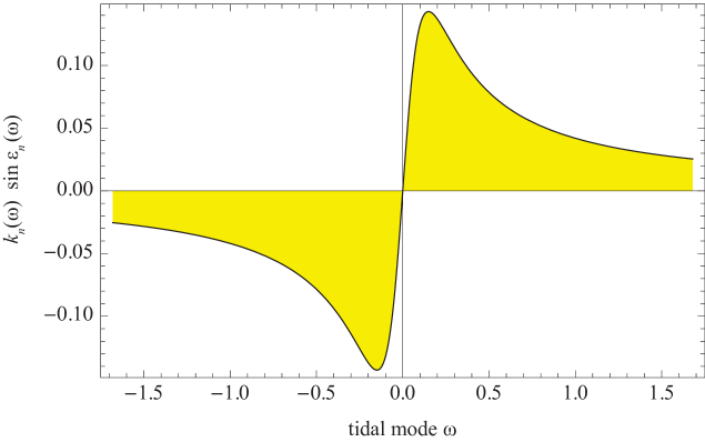
For the Maxwell or Andrade model, the dependence of $~{}K_{n}\nobreak\hskip 1.1pt\nobreak\equiv\nobreak\hskip 1.1pt\nobreak k_{\textstyle{{}_{n}}}~{}\sin\epsilon_{\textstyle{{}_{n}}}\,$ on a tidal mode has the shape of a kink, depicted in Figure 5. It can be demonstrated (Efroimsky, 2015, eqn 45) that the frequency-dependence of the inverse quality factor $\nobreak\hskip 1.1pt\nobreak Q_{n}(\chi)^{-1}\;\equiv\;|\nobreak\hskip 1.1pt\nobreak\sin\epsilon_{n}(\chi)\nobreak\hskip 1.1pt\nobreak|\nobreak\hskip 1.1pt\nobreak$ has a similar shape, with a similarly positioned peak.

For a Maxwell body, the extrema of the kink $\,K_{n}(\omega)\,$ are located at

$${\omega_{peak}}_{\textstyle{{}_{n}}}\,=\;\pm\;\;\frac{\tau_{M}^{-1}}{1\,+\,{\cal{B}}_{n}\,\mu}\;\approx\;\pm\;\frac{1}{{\cal{B}}_{n}\,\eta}\,\;,$$ (61)

which can be checked by insertion of formulae (7 - 8) into equation (60). 

Between the peaks, the quality function $\,K_{n}(\omega)=k_{n}(\omega)\,\sin\epsilon_{n}(\omega)\,$ is about linear in frequency: 

$$|\nobreak\hskip 1.1pt\nobreak\omega\nobreak\hskip 1.1pt\nobreak|\;<\;|\nobreak\hskip 1.1pt\nobreak{\omega_{peak}}_{n}\nobreak\hskip 1.1pt\nobreak|\quad\Longrightarrow\quad K_{n}(\omega)\;\approx\;\frac{3}{2\nobreak\hskip 1.1pt\nobreak(n-1)}\;\frac{\omega}{|\nobreak\hskip 1.1pt\nobreak{\omega_{peak}}_{n}\nobreak\hskip 1.1pt\nobreak|}\,\;.$$ (62)

Outside the inter-peak interval, the function $\,K_{n}(\omega)\,$ falls off as the inverse frequency:

$$|\nobreak\hskip 1.1pt\nobreak\omega\nobreak\hskip 1.1pt\nobreak|\;>\;|\nobreak\hskip 1.1pt\nobreak{\omega_{peak}}_{n}\nobreak\hskip 1.1pt\nobreak|\quad\Longrightarrow\quad K_{n}(\omega)\;\approx\;\frac{3}{2\nobreak\hskip 1.1pt\nobreak(n-1)}\;\frac{|\nobreak\hskip 1.1pt\nobreak{\omega_{peak}}_{n}\nobreak\hskip 1.1pt\nobreak|}{\omega}\;\;.$$ (63)

Naturally, the insertion of $\,\omega={\omega_{peak}}_{n}\,$ in any of these expressions renders the same value for the peak amplitude:

$$K_{n}^{\rm{(peak)}}\nobreak\hskip 1.1pt\nobreak\approx\;\pm\;\frac{3}{2\nobreak\hskip 1.1pt\nobreak(n-1)}\,\;.$$ (64)

While the peaks’ amplitude is insensitive to a choice of the viscosity value $\nobreak\hskip 1.1pt\nobreak\eta\nobreak\hskip 1.1pt\nobreak$, the spread between the extrema depends on $\nobreak\hskip 1.1pt\nobreak\eta\nobreak\hskip 1.1pt\nobreak$. Expression (61) indicates that for a higher viscosity the peaks are residing close to zero, i.e. to the point of resonance $\omega\equiv\omega_{nmpq}=0$. If the viscosity evolves and assumes lower values (which happens when a body is getting warmer), the peak frequency grows, eventually superseding the orbital frequency $\nobreak\hskip 1.1pt\nobreak\dot{\cal M}\nobreak\hskip 1.1pt\nobreak$. In realistic situations, this requires very low viscosities and happens for bodies at high temperatures or, possibly, for bodies close to rubble. Outside the inter-peak interval, the quality function $\,K_{n}(\omega)\,$ behaves as $\,\sin\epsilon_{n}(\omega)=Q^{-1}_{n}(\omega)\,\mbox{Sign}(\nobreak\hskip 1.1pt\nobreak\omega\,)$, and its values change slowly with frequency.

Owing to the near-linear mode-dependence of $K_{n}$ in the inter-peak interval, the tidal torque value transcends spin-orbit resonances continuously (Makarov and Efroimsky, 2013; Noyelles et al., 2014).  From expression (45) in Efroimsky (2015), it can be derived that for a Maxwell body with $\nobreak\hskip 1.1pt\nobreak{\cal B}_{n}\nobreak\hskip 1.1pt\nobreak\mu\gg 1\nobreak\hskip 1.1pt\nobreak$, the locations of extrema of the kink function $\,\sin\epsilon_{n}(\omega)=Q^{-1}_{n}(\omega)\,\mbox{Sign}(\nobreak\hskip 1.1pt\nobreak\omega\,)$ virtually coincide with the locations of the extrema (61) for $\nobreak\hskip 1.1pt\nobreak K_{n}\nobreak\hskip 1.1pt\nobreak$. Each of these two functions has only one peak for a positive tidal mode, when the regular Maxwell or Andrade models are used. This changes if we insert into formula (60), and into its counterpart for $\,\sin\epsilon_{n}(\omega)=Q^{-1}_{n}(\omega)\,\mbox{Sign}(\nobreak\hskip 1.1pt\nobreak\omega\,)$, a complex compliance corresponding to a more elaborate rheology, such as the Sundberg-Cooper one. In that situation, an additional peak will appear.

4.5 Layered bodies

Analytical solutions for the tidal response of a homogeneous planetary body using other viscoelastic models can be derived (Renaud and Henning, 2018). However, in most geophysical applications, more sophisticated modeling is required for precise interpretations. This is due to the fact that the material properties of the planetary bodies vary with depth. This results in variation of the tidal response of the planetary body compared to a homogeneous planet. The variation of temperature, pressure, and grain size within the planetary bodies can be taken into account using the viscoelastic models discussed in Section 2. Such an approach has been followed by, e.g., Bagheri et al. (2022, 2019); Khan et al. (2018); Nimmo et al. (2012); Nimmo and Faul (2013); Padovan et al. (2014); Steinbrügge et al. (2021); Plesa et al. (2018). To model a layered planetary body with depth-dependent properties, numerical methods have been used in such studies (Tobie et al., 2008; Roberts and Nimmo, 2008; Běhounková et al., 2015), while another widely used class of methods is based on the propagator matrix technique, derived in the scope of the normal mode theory (e.g., Alterman et al., 1959; Takeuchi et al., 1962; Wu and Peltier, 1982; Vermeersen et al., 1996; Sabadini and Vermeersen, 2004). Similar approach is used to calculate the tidal response by, e.g., Plesa et al. (2018); Moore and Schubert (2000); Padovan et al. (2014) to obtain the interior structure models further discussed in Section 5. Martens et al. (2016) developed a Python toolbox to compute the tidal and load Love numbers in an elastic regime and exploited it (Martens et al., 2019) to study the Earth’s tides. Bagheri et al. (2019) used a numerical code based on the spectral-element-method to compute the tidal response using several viscoelastic models. Dmitrovskii et al. (2021) used the same technique in 3D to model tides in an irregularly shaped body (Phobos); but only modeled the elastic response instead of a general viscoelastic behaviour.

The overall tidal response of layered bodies depends on the interplay between the individual layers. For example, an ocean or a global molten layer below the crust or lithosphere might effectively decouple the interior of the planet from the surface and diminish the tidal deformation of the lower layers.

Figure 6: The inverse tidal quality factor of a model Earth-sized planet with a liquid core, a mantle of viscosity $10^{21}\,\mathrm{Pa\;s}$ and rigidity $\mu=200\,\mathrm{GPa}$, and a weak surface layer (e.g., a global icy crust). The left panel illustrates the effect of the upper layer’s viscosity, keeping its thickness fixed to $200\,\mathrm{km}$ and its rigidity to the mantle value. On the right panel, the layer’s viscosity is held constant at $10^{17}\,\mathrm{Pa\;s}$ and the individual lines correspond to different thicknesses.

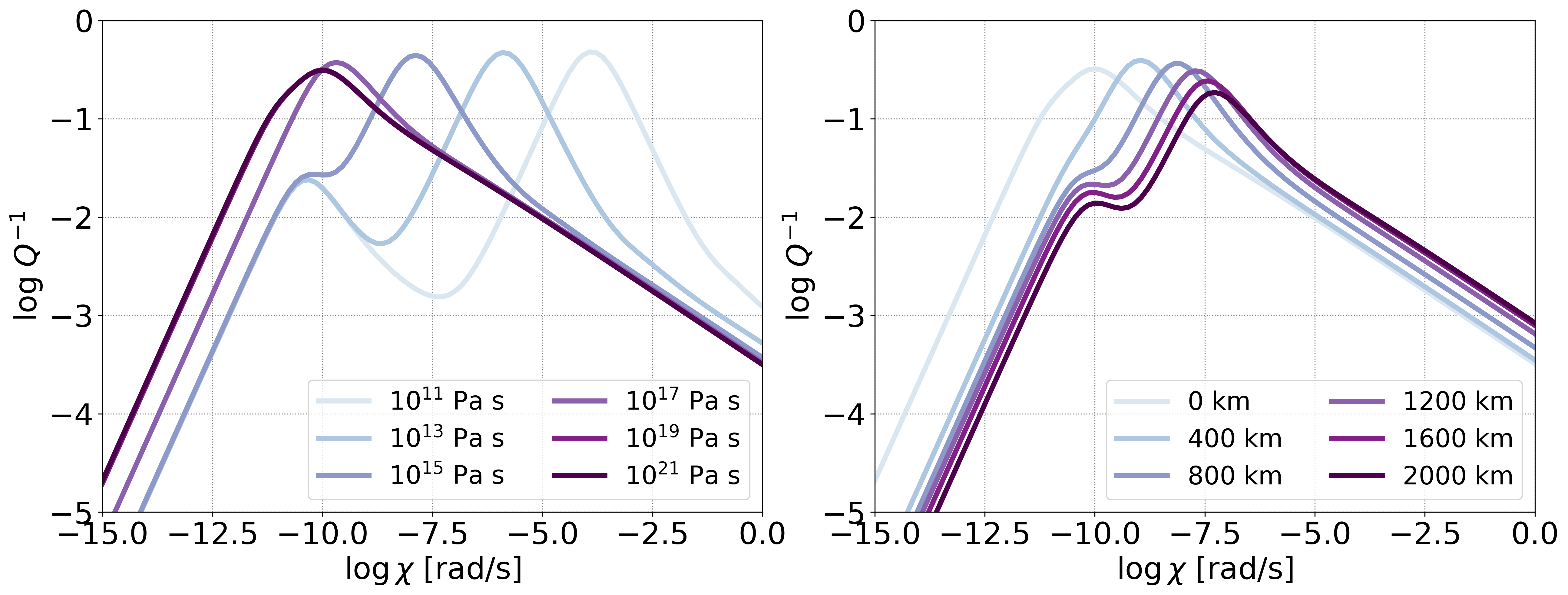
As an instructive example, a comparison between the tidal response of a planetary body incorporating layers of different physical properties is shown in Figure 6. This figure depicts the tidal quality factor of a three-layered Earth-sized planet consisting of a liquid core, a solid mantle governed by the Andrade rheology, and a weak surface layer with the same properties as the mantle, but a lower viscosity. The presence of two dissipative layers leads to the emergence of two peaks in the $Q^{-1}$ spectrum. In this sense, the response of a layered body might be mimicked by an advanced rheological model, for example the Sundberg-Cooper rheology (Gevorgyan, 2021) or by its extensions. Moreover the peak corresponding to the planetary mantle is shifted to higher frequencies and it becomes weaker with decreased upper-layer viscosity (or increased upper-layer thickness).

Appropriately modeling the tidal response on the layered bodies can also help in understanding the the tidal dissipation pattern (e.g., Beuthe, 2013), and interpret them to infer knowledge about the interior properties. As shown by Segatz et al. (1988) in the case of Jovian moon Io, the presence of a semi-molten layer (an astenosphere) between the solid mantle and lithosphere can considerably affect the pattern of surface tidal heat flow. The same is true for the tidal dissipation within icy moons with a subsurface ocean (Tobie et al., 2005b) and for hypothetical exoplanets with icy crust overlying a silicate mantle (Henning and Hurford, 2014).

5 Tides as a probe of the deep interior

Having introduced the theoretical aspects of modeling tides in previous sections, here we address particular planetary bodies, focusing on how information about their interiors was obtained by studying their tidal response. We summarise the constraints on the interior properties of Mercury, Venus, the Moon, Mars and its moons, and the largest moons of giant planets. We also mention the expected future improvements in measuring these bodies’ tidal response.

5.1 Mercury

Studies of Mercury’s interior have long focused on its magnetic and gravitational field, and only recently the first measurements of its tidal response were obtained. The Mariner 10 flybys in 1974 and 1975 (Dunne, 1974) provided us with the first clues of Mercury’s interior, by detecting its magnetic field (Ness et al., 1974), and with the first measurements of its gravitational field (Anderson et al., 1987). A much more detailed view of Mercury and its environment was provided by NASA’s MErcury Surface, Space ENvironment, GEochemistry, and Ranging (MESSENGER) spacecraft, the first to orbit Mercury (Solomon et al., 2007). Pre-MESSENGER studies of Mercury often focused on a combination of rotation and tides, together with its spin-orbit resonance, providing predictions that could later be tested against MESSENGER data (Van Hoolst and Jacobs, 2003; van Hoolst et al., 2007; Rambaux et al., 2007; Rivoldini et al., 2009; Dumberry, 2011; Matsuyama and Nimmo, 2009).

One of MESSENGER’s many goals was to map Mercury’s gravity field, which could then be used to determine the state of Mercury’s core. Peale (1976) and Peale et al. (2002) showed that, because Mercury is in a Cassini state (where its spin axis, its orbit normal, and the normal to the invariable plane are co-planar), its polar moment of inertia and the moment of inertia of the solid outer shell (mantle and crust) can be determined from 3 quantities: Mercury’s obliquity, the amplitude of its longitudinal librations, and its second degree gravitational harmonic coefficients. The first two were determined from Earth-based radar data (Margot et al., 2007), and MESSENGER finally provided the first precise measurement of Mercury’s second degree harmonics (Smith et al., 2012). During the MESSENGER mission, estimates of its gravity field were updated as more data were collected. Mercury’s gravitational tidal response as expressed in its degree two Love number $k_{2}$ was also determined.

Figure 7: The view of Mercury’s interior based on recent measurements of its rotational state. Adapted from Genova et al. (2019).

The first estimate of $k_{2}=0.451\pm 0.014$ was reported by Mazarico et al. (2014b) using three years of MESSENGER radio tracking data. The Love number was co-estimated along with gravity field parameters and rotational parameters, but they found that the radio data was not sensitive to parameters describing the forced librations. The value of $k_{2}$ was consistent with pre-MESSENGER analyses of Mercury’s tidal response, which indicated a range of 0.4 – 0.6 (Van Hoolst and Jacobs, 2003; Rivoldini et al., 2009). Using the newly determined gravitational parameters, Rivoldini and van Hoolst (2013) and Hauck et al. (2013) investigated Mercury’s interior structure as constrained by its moments of inertia, but without considering the tides.

Initial results using MESSENGER data proposed the existence of an FeS layer on top of the core, to account for the higher mantle density that was a result of a larger-than-expected value for the moment of inertia of the outer shell (Smith et al., 2012). Results using MESSENGER’s X-Ray Spectrometer measurements of the ratio of Ti and Si also argue against the FeS layer (Cartier et al., 2020). Mercury’s core itself is mostly considered to be metallic, with light elements of S and/or Si (Rivoldini et al., 2009; Hauck et al., 2013; Chabot et al., 2014; Knibbe and van Westrenen, 2015, 2018).

Padovan et al. (2014) were the first to comprehensively consider Mercury’s tidal response in the light of MESSENGER’s results. They considered several end-member models such as a hot or cold mantle, and found that the results presented in Mazarico et al. (2014b) fell in their range, and would be mostly consistent with their cold mantle, without a layer of FeS on the top of the core. The latter was initially considered by Smith et al. (2012) to account for the relatively large moment of inertia of the outer shell. Updates to the estimate of Mercury’s obliquity by Margot et al. (2012) reduced this value, and an FeS layer was no longer necessary (Hauck et al., 2013; Rivoldini and van Hoolst, 2013; Knibbe and van Westrenen, 2015). The $k_{2}$ value was also later confirmed by an independent analysis by Verma and Margot (2016), with a value of $k_{2}=0.464\pm 0.023$. Steinbrügge et al. (2018) further investigated Mercury’s tidal response, and computed models consistent with MESSENGER measurements of mean density, mean moment of inertia, moment of inertia of mantle and crust, and $k_{2}$. They showed that the ratio of $h_{2}$ (the radial displacement Love number) and $k_{2}$ can provide better constraints on the size of a possible solid inner core than the geodetic measurements such as moments of inertia can.

The MESSENGER mission had several extensions, where the altitude and location of its periapsis changed, with lower and lower altitudes obtained in the northern hemisphere, down to 25 km above surface. This increased the sensitivity of the tracking data with respect to smaller scale gravity features, and to Mercury’s tidal response. Using the entire set of tracking data, Genova et al. (2019) presented a gravity model that included estimation of Mercury’s rotational parameters and tidal Love number. Their estimate of Mercury’s obliquity unambiguously satisfies the Cassini state. Their obliquity value results in a lower normalised polar moment of inertia of $0.333\pm 0.005$, whereas earlier results yielded normalised polar moment of inertia values around 0.346 (Margot et al., 2012; Hauck et al., 2013; Mazarico et al., 2014b). Using this updated value and smaller error, they modeled Mercury’s interior with a Markov Chain Monte Carlo (MCMC) (Mosegaard and Tarantola, 1995) approach and found evidence for the existence of a solid inner core, with the most likely core size being between 0.3 and 0.7 times the size of the liquid core. Their updated Love number, $k_{2}=0.569\pm 0.025$, was also higher than the previous estimate.

An analysis by Bertone et al. (2021) also finds Mercury’s rotational parameters unambiguously satisfying the Cassini state, yet with a different obliquity that results in a normalised polar moment of inertia value of $0.343\pm 0.006$. Their analysis is based on laser altimetry data from the Mercury Laser Altimeter (MLA, Cavanaugh et al. (2007)), using crossovers (where two laser tracks intersect, the difference in measured altitude can be used to infer rotation and tidal parameters, for example). This discrepancy could point to differences in the rotation state of the entire planet as measured by gravity and the rotation state of the outer shell as measured by laser altimetry. Bertone et al. (2021) did not estimate $k_{2}$ but they did provide the first estimate of the radial displacement Love number, $h_{2}=1.55\pm 0.65$. Due to the sparsity of crossovers, this parameter is difficult to measure. Finally, an analysis by Konopliv et al. (2020), using the entire MESSENGER tracking data set, determined Mercury’s Love number in close agreement with that of Genova et al. (2019), with a value of $k_{2}=0.53\pm 0.03$.

The differences in moment of inertia values and newly determined Love numbers have implications for our knowledge of Mercury’s interior structure, especially for the size of the liquid core. Steinbrügge et al. (2021) performed an analysis of the lower normalised polar moment of inertia value of 0.333 and the higher Love number of 0.569, and found several challenges in determining interior structure models that fit these parameters: they find a relatively large inner core (> 1000 km), a relatively high temperature at the core-mantle boundary (CMB; above 2000 K), low viscosities at this boundary (below $10^{13}$ Pa s), and a low mantle density (markedly below 3200 kg m^-3). They also indicate that the low viscosities required to match $k_{2}$ imply a significantly weaker mantle. They indicate that such challenges do not exist for the higher normalised polar moment of inertia value of $\sim 0.346$. It should be noted that they focused their analysis on models that matched the central values of parameters such as the moments of inertia and $k_{2}$. If they take into account the quoted errors, they indicate some of the challenges are alleviated.

Figure 8: Results of the MCMC analysis by Goossens et al. (2022), which determined models of Mercury’s interior structure using different measurements for the normalised polar moment of inertia and tidal Love number $k_{2}$. The label “G19" refers to Genova et al. (2019) and “M14" to Mazarico et al. (2014b). The results are shown as heatmaps of the mapped quantities for all accepted models in the MCMC analysis. For the top panels, $k_{2}$ was used as a measurement in the MCMC analysis, whereas it was predicted for the results in the bottom panels. These results indicate that the set of measurements of G19 s the most consistent. Higher values of the normalised polar moment of inertia, as provided by M14, cannot simultaneously fit the measured $k_{2}$, and would indeed predict an even higher value.

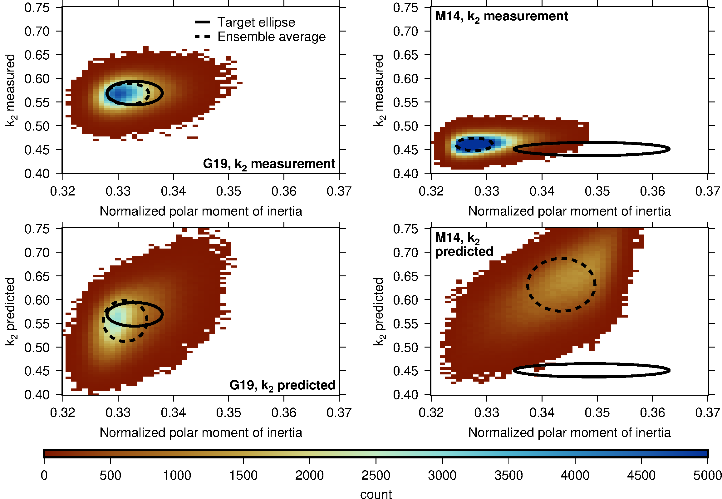
A recent analysis by Goossens et al. (2022) also investigated the different values for moments of inertia and $k_{2}$, using an MCMC method to map out models of Mercury’s interior that satisfy the measurements and their quoted errors. They find that models that match the lower normalised polar moment of inertia value of 0.333 (Genova et al., 2019) also match or predict the Love number value of $k_{2}=0.569$. Models that match the higher normalised polar moment of inertia of $\sim 0.346$ indicate even higher Love numbers, larger than 0.6, with a wide spread. Their study thus indicates that the higher normalised polar moment of inertia values are not consistent with the current measurements of the Love number. In addition, they also find lower CMB temperatures than Steinbrügge et al. (2021) indicated, in the range of 1600 – 2200 K but with a peak at 1800 K. While their study does indicate low viscosity values at the CMB, models with a constant mantle temperature, mimicking a convecting mantle rather than a conducting one, predict lower temperatures and higher viscosities. Models that satisfy the lower normalised polar moment of inertia and the updated moment of inertia for the outer shell do indicate mantle densities that are lower than previously assumed ($3089\pm 135$ kg m^-3). A study by Lark et al. (2022) indicates that the presences of sulfides in the mantle can explain this lower density. Goossens et al. (2022) also provide a prediction for the radial displacement Love number $h_{2}=1.02\pm 0.04$ for models that satisfy the measurements from Genova et al. (2019).

The next spacecraft that will orbit Mercury is the European Space Agency’s BepiColombo mission (Benkhoff et al., 2010). This spacecraft will provide precise gravity measurements (Genova et al., 2021) as well as laser altimetry (Thomas et al., 2021), both with a more global coverage than was possible with MESSENGER, due to the latter’s elliptical orbit around Mercury. BepiColombo data will provide updated measurements of the moments of inertia and the Love numbers $k_{2}$ and $h_{2}$ (Steinbrügge et al., 2018; Thor et al., 2020; Genova et al., 2021), as well as for its rotational state and gravity, which will help resolve the current challenges in understanding Mercury’s interior structure.

5.2 Venus

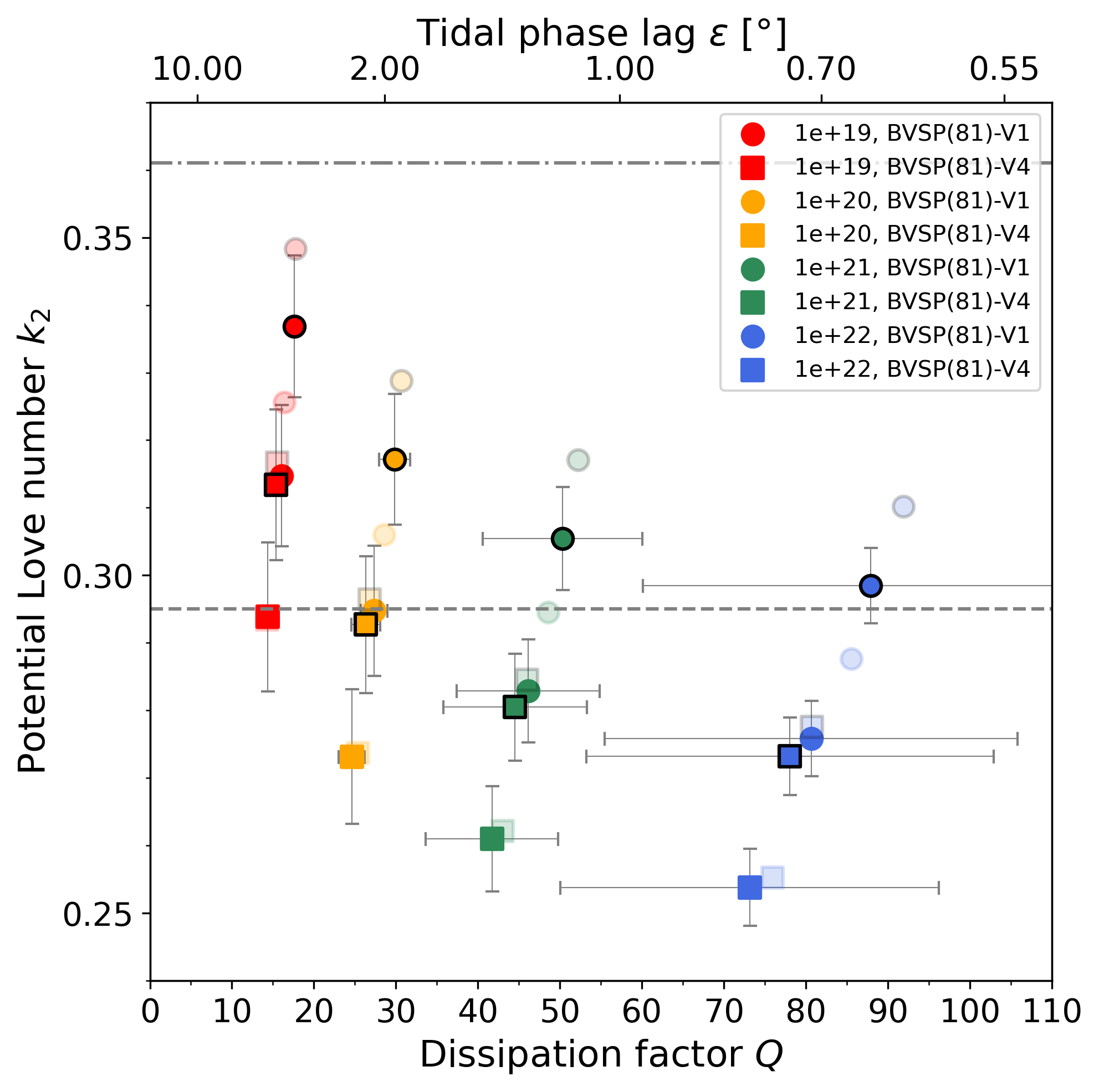
The tidal response of Venus to semi-diurnal Solar tides was measured more than a quarter century ago using Magellan and Pioneer tracking data. Konopliv and Yoder (1996) estimated the $2$-$\sigma$ interval for the potential Love number as $k_{2}=0.295\pm 0.066$ and concluded, following the predictions of Yoder (1995), that Venus has a fully liquid core. However, this conclusion was based on a purely elastic model of the tidal response. A new reassessment of the problem with a compressible Andrade model (Dumoulin et al., 2017) indicated that the question of size and state of the Venusian core cannot be resolved with the data available. The wide range of admissible Love numbers, combined with the absence of $Q$ measurements and with the large uncertainties on the planet’s moment of inertia (Margot et al., 2021) constrains neither the core state, nor the mantle mineralogy and temperature profile. Dumoulin et al. (2017) illustrated that only a future measurement of $k_{2}$ below $0.26$ and a large phase lag ($\epsilon_{2}>4^{\circ}$) would indicate a fully solid core. At higher Love numbers, the core can be interpreted as at least partially liquid and a precise measurement of the phase lag would further help to discern between different mantle viscosities and thermal states (see Figure 9).

Figure 9: Left: Overview of Venusian tidal parameters for two mantle mineralogies and two mantle temperature profiles, assuming an incompressible Andrade model, reproduced after Dumoulin et al. (2017). Circles symbolise an iron-poor ($0.24$ wt$\%$ FeO) mantle model and squares an iron-rich ($18.7$ wt$\%$ FeO) model according to Basaltic Volcanism Study Project (1981). Different colours stand for different mantle viscosities; the markers with black edges correspond to a hot interior (Armann and Tackley, 2012) and the markers without contour correspond to a cold interior (Steinberger et al., 2010). The dashed and dot-dashed lines indicate the mean value and the upper bound of the $2$-$\sigma$ interval for the tidal Love number obtained by Konopliv and Yoder (1996) using Magellan and Pioneer data: $k_{2}=0.295\pm 0.066$. Finally, the error bars illustrate the span of results calculated for different values of the Andrade parameter $\alpha\in(0.2,0.3)$ (see Section 2.5), and the transparent markers, taken from Dumoulin et al. (2017), indicate the effect of compressibility. Right: Schematic interior structure of Venus from Shah et al. (2022)

In addition to solid-body tides, the deformation of Venus is also affected by atmospheric tides consisting of two components: one due to the gravitational loading by the Sun and the other resulting from thermal forcing (Auclair-Desrotour et al., 2017; Correia et al., 2003; Ingersoll and Dobrovolskis, 1978; Gold and Soter, 1969). The interplay between the gravitational and thermal tides leads to the instability of synchronous rotation and it has probably driven the planet to its present-day retrograde spin configuration. Close to its nonsynchronous, yet stationary rotation state, Venus might also be influenced by the weak gravitational pull of the Earth, as hypothesised by Dobrovolskis and Ingersoll (1980) and Gold and Soter (1969). Besides the contribution to the planet’s rotational dynamics, the atmosphere acts as a global surface load and diminishes the tidal deformation of the Venusian surface by approximately $0.3\%$ (see Remus et al., 2012; Dermott, 1979).

The tidal phase lag and thus the tidal quality factor $Q$ can also be used to constrain the thermal state of the interior, given the temperature dependence of the mantle viscosity. In addition to the present-day values, knowing the past thermal state and $Q$ of Venus can further help us to understand its tidally-induced rotational evolution (Bolmont et al., 2020). Since Venus and the Earth are often referred to as twin planets, due to their similar size and mass, the tidal quality factor $Q$ may be similar between the two bodies. However, while on the Earth plate tectonics represent an efficient way to cool the interior, on Venus large scale subduction may be absent today. In fact, a recent study by Rolf et al. (2018) concluded that if Venus may have experienced one or multiple episodes of plate tectonics in the past, the last of those episodes likely ended 300-450 Myr ago, otherwise thermal evolution models cannot match the observed surface gravity spectrum. If Venus has been in a stagnant lid regime, with an immobile surface over the past 500 Myr, its interior would likely have a much higher temperature than that of the present-day Earth. This may indicate a much more dissipative interior, i.e. lower tidal quality factor $Q$, than that of the solid Earth, for which $Q$ is around 280 (Ray et al., 2001). Even if Venus currently experiences some sort of surface mobilisation on a much smaller scale than tectonic plates provide on the Earth, with small patches of the surface being recycled in the interior (i.e., the so-called plutonic squishy lid regime Lourenço et al. (2020)), this might still lead to a hotter interior than on present-day Earth. This type of surface mobilisation is thought to have operated on the Earth in the past during the Archean, when the interior temperature were higher than they are today (Rozel et al., 2017; Lourenço et al., 2020).

That the interior of Venus may be characterised by high mantle temperatures, which in turn may indicate a higher dissipation, is also supported by the small elastic lithosphere thickness that are indicators for a thin and hot lithosphere (Smrekar et al., 2018). Small elastic thicknesses are estimated at coronae (O’Rourke and Smrekar, 2018), steep side domes (Borrelli et al., 2021), and crustal plateaus (Maia and Wieczorek, 2022), and likely 20 km or less may be representative for a significant part of the planet (Anderson and Smrekar, 2006). Moreover, the temperatures inside the Venusian mantle may allow for volcanic activity at present-day. This has been suggested by several observations. For example, the presence of recently active hot-spots in the interior of Venus has been inferred based on their thermal signature (Shalygin et al., 2015) and emissivity data of Venus Express, which allow to distinguish fresh from weathered basaltic material (Helbert et al., 2008; Smrekar et al., 2010; D’Incecco et al., 2017). In addition, gravity, topography and surface deformation structures at the locations where recent volcanic activity has been suggested are consistent with the presence of mantle plumes in the interior (Kiefer and Hager, 1991; Smrekar and Phillips, 1991). Furthermore, SO₂ variations in the atmosphere of Venus recorded by Pioneer Venus Orbiter (Esposito, 1984; Esposito et al., 1988) and later by Venus Express (Marcq et al., 2013) provide additional hints at recent volcanic activity. All this evidence, although indirect, may indicate that the present-day interior of Venus is characterised by high mantle temperatures and hence low mantle viscosities that would lead to a lower dissipation factor than that of the Earth. Whether the above conclusions hold or not, it needs to be tested by future data that would allow to place tighter constraints on the thermal state of the Venusian interior.

Owing to the lack of recent and accurate tidal measurements, Venus still remains the most enigmatic of terrestrial worlds. Recently revived interest in its interior and atmospheric conditions, nurtured by the putative detection of biosignatures (Greaves et al., 2021; cf. Villanueva et al., 2021), foreshadowed the selection of two geophysical mission concepts for a launch in late 2020s or early 2030s. The VERITAS mission (Venus Emissivity, Radio Science, InSAR, Topography, and Spectroscopy; Smrekar et al., 2020) of NASA’s Discovery Program will address the present geological and volcanic activity, the link between interior and atmospheric evolution, and the global accurate mapping of Venusian gravity field. In order to reduce the uncertainties of the gravity field (and tidal response) measurements, introduced by the planet’s rotation, the mission will combine standard Earth-based Doppler tracking with the systematic observation of surface features by the onboard instrument VISAR (Venus Interferometric Synthetic Aperture Radar). With this approach, the expected $3$-$\sigma$ accuracy of the Love number $k_{2}$ is $4.6\times 10^{-4}$ and of the tidal phase lag $0.05^{\circ}$ (Cascioli et al., 2021).

The medium-sized ESA’s Cosmic Vision Programme mission EnVision (Ghail et al., 2016) will focus on the geological structures of Venus that are of interest for understanding its past thermal evolution. As in the case of VERITAS, the primary objectives of the mission also include the determination of a uniform high-resolution gravity field, with a spatial resolution better than $\sim 170\,\mathrm{km}$. The expected $1$-$\sigma$ error of both the real and the imaginary parts of the Love number $k_{2}$ is $10^{-3}$, implying a $0.1^{\circ}$ uncertainty for the tidal phase lag (Rosenblatt et al., 2021). Despite the similarity of the two geophysical missions, VERITAS and EnVision are expected to be synergistic. First, the launch of EnVision is planned for a later date than the launch of VERITAS, and the two orbiters will only operate simultaneously for a part of the respective mission durations. Second, while VERITAS aims at providing a global geophysical survey, EnVision is designed for more targeted, repeated observations of the regions of interest identified by the former (Ghail, 2021). With the new data, a refined estimate of the Venusian core size will be possible and the first measurements of phase lag will enable constraining the average mantle viscosity within an order of magnitude (Dumoulin et al., 2017; Rosenblatt et al., 2021).

5.3 The Moon

The Moon is one of the best studied bodies in the Solar system because of its proximity to the Earth. It is only 60 Earth radii away and its surface undergoes a monthly tidal deformation of $\pm$ 0.1 m generated by the Earth’s gravitational field. This tidal potential impacts also the Moon’s gravity field and its orientation periodically. In addition, the Moon does not have an ocean as on the Earth and the tidal variations are only incorporated in solid tides. These variations are detected by space missions orbiting the Moon and by Lunar-Laser Ranging measurements performed from the stations on the Earth. These accurate regular measurements over the past 50 years have made the Moon the best place to test tidal theory and dissipation mechanisms. The interpretation of these variations provides information about the lunar interior, but many questions remain about its internal structure and dissipation mechanisms.

The determination of the Love number $k_{2}$ at the monthly period of the Moon (its orbital period) has most recently been obtained by the Gravity Recovery and Interior Laboratory (GRAIL) space mission radio science experiment, which consists of precise measurements of two satellites in orbit around the Moon (Zuber et al., 2013). The link between the satellites is in Ka-band and the link to the ground stations in S-band. This experiment is similar to the GRACE mission around the Earth and GRAIL has determined the lunar gravity field up to degree 900 (Konopliv et al., 2014) and provided the monthly Love $k_{2}$ number of the Moon at 0.02416 $\pm$ 0.00022 (Konopliv et al., 2013, 2014; Lemoine et al., 2013; Williams et al., 2014). The Love number $h_{2}$ is determined on the Moon using the Lunar Reconnaissance Orbiter mission which carries a laser altimeter, Lunar Orbiter Laser Altimeter LOLA which measures displacements of the Moon’s surface to an accuracy of 10 cm (Smith et al., 2017). The Moon’s Love number $h_{2}$ is determined to be 0.0371 $\pm$ 0.0033 (Mazarico et al., 2014a) and 0.0387 $\pm$ 0.0025 (Thor et al., 2021). Finally, the dissipation of the Moon is extracted from LLR ranging measurements by analysing the lunar orientation and libration (Park et al., 2021; Pavlov et al., 2016; Viswanathan et al., 2018) and see reference therein). The Lunar-Laser Ranging (LLR) consists of precise measurements of the round-trip travel time of a photon emitted from a laser on an Earth-ground station and lunar retroreflectors deployed by US astronauts and the Russian Lunakhod robotic missions (Murphy, 2013; Chabé et al., 2020). These measurements allow to determine the Earth-Moon distance centimeter level and the lunar rotation to the milli-arcsecond level (Viswanathan et al., 2018; Park et al., 2021). Lunar orientation and libration analysis allows for extraction of the lunar dissipation. Currently, the monthly lunar tidal bulge delay time is estimated to be 0.1 days which corresponds to a monthly dissipation factor Q = 38 (Williams et al., 2001; Williams and Boggs, 2015).

Beyond the monthly Love number $k_{2}$ and dissipation factor $Q$, precise analyses of the LLR data have determined their frequency dependence. Indeed, the Moon’s orbit is strongly perturbed by the presence of the Sun and its orbital motion results from a three-body motion. The Moon’s orbit is described according to the Delaunay arguments $\ell$, $\ell^{\prime}$, $F$, $D$ which represent the mean anomaly of the Moon, the mean anomaly of the Earth-Moon barycentre, the latitude anomaly of the Moon and the elongation of the Moon of periods 27.55 days, 365.25 days, 27.21, 29.53 days, to which must be added the precession of the lunar orbit of 18.6 years (for a description of the lunar orbit see Chapront-Touzé and Chapront (1988, 1991). Thus, librations and tidal shifts are mixed and tidal frequencies appear as mixed combinations of these frequencies with a period spectrum ranging from 2 weeks to 18.6 years and frequencies at 1 month, 7 months and 1 year (Williams et al., 2001; Rambaux and Williams, 2011; Williams and Boggs, 2015). The extraction of dissipation factors from LLR fits and the orientation of the Moon is challenging, but the terms at 27.2 days and 365 days stand out, while two others at 1095 and 2190 days provide upper bounds on lunar dissipation, whereas the term at 206 days is very complicated (Williams et al., 2001; Williams and Boggs, 2015). The $k_{2}/Q$ curve as a function of period has a kinked shape as shown in Section 2, and the rheological models can then be compared with the observations to identify plausible internal structure patterns (Williams and Boggs, 2015).

Several rheological models, such as Maxwell, Andrade, absorption band (See Figure 10), were employed to explain the relatively low monthly dissipation factor Q=38 and the bell-shaped behaviour of the $k_{2}/Q$ law (see e.g., Williams and Boggs, 2015). Three physical mechanisms to explain this dissipation have been suggested: (i) the properties of the lunar material, (ii) the presence of water at depth and (iii) the presence of a partially molten zone.

(i) By analogy with the Earth, Nimmo et al. (2012) examined the influence of polycrystalline olivine melt-free to explain the observed dissipation. They were able to reproduce the dissipation at seismic and monthly tidal frequencies but not the slope behaviour associated at longer tidal periods. Matsuyama et al. (2016) developed a Bayesian approach to test the presence or not of a transient layer above the core from the observed mass, solid moment of inertia, and elastic Love numbers $k_{2}$ and $h_{2}$ to constrain the density and rigidity profile of the Moon. Their model favors an internal structure without a transition zone. However, it should be noted that this observation is based on a purely elastic approach. Matsumoto et al. (2015) adopted a similar approach to Matsuyama et al. (2016) to study the interior of the Moon using an MCMC method. Their results are slightly different than Matsuyama et al. (2016) in that, for example, Matsuyama et al. (2016) obtain a unimodal probability distribution for the liquid outer core radius, while Matsumoto et al. (2015) obtained a bimodal distribution. Matsuyama et al. (2016) attribute this difference to the ways of computing the Love numbers, i.e., Matsuyama et al. (2016) apply a simple anelastic correction to the observed Love numbers, while Matsumoto et al. (2015) use a viscoelastic model to compute the Love numbers at the tidal forcing period, or, alternatively, to the use of additional tidal quality and seismic constraints by Matsumoto et al. (2015).

(ii) Karato (2013) proposed that water concentration would be the mechanism behind dissipation, also by analogy with the Earth’s asthenosphere. Although this model reproduces the low value of the dissipation factor it does not describe the frequency dependence.

(iii) Finally, the molten layer model proposed by Nakamura as early as 1973 from seismic data seems to be the most robust. A Bayesian approach developed by Khan et al. (2014) used Love number, mass distribution, composition and electromagnetic data to explore the parameter space and conclude that the melt layer is present. Later, an attempt to fit the LLR data to the power scaling law $\,Q\sim\chi^{p}\,$ resulted in a small negative value of the exponential: $\,p\,=\,-\,0.19~{}$ (Williams et al., 2001). A subsequent reprocessing of the data in (Williams and Boggs, 2009) rendered the value $\,p\,=\,-\,0.07~{}$. Efroimsky (2012) proposed that since the frequency-dependence of $Q^{-1}$ has a kink form, as in Figure 5, the negative slope found by the LLR measurements may be located slightly to the left of the pick of the kink. For a Maxwell Moon, this necessitates the mean viscosity as low as $\sim\nobreak\hskip 1.1pt\nobreak 3\times 10^{15}\nobreak\hskip 1.1pt\nobreak$ Pa s, implying the presence of a considerable amount of partial melt. More recently, various models were used to explain by a partially molten layer the LLR data on the frequency dependence of dissipation (e.g., Harada et al., 2014, 2016; Rambaux et al., 2014; Williams and Boggs, 2015; Tan and Harada, 2021; Briaud, 2022).

Figure 10: Top: Artistic view of the interior structure and surface features of the Moon; Bottom: Frequency dependence of k2/Q for various lunar rheological models (in colors) and LLR measurements points and limits (in black). The absorption band and Debye model presents a kink reproducing the measurements (figure from Williams and Boggs (2015)"

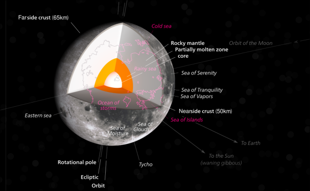
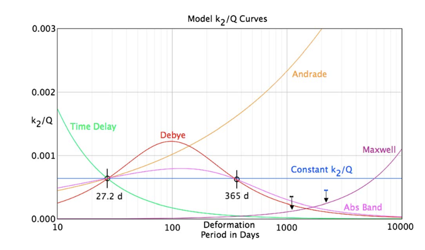
We are at the beginning of the study of lunar dissipation, and our knowledge is still fragmentary. Several directions of improvement are now possible. Firstly, from an observational point of view, the installation of new, more compact and optimised single lunar Cube Corner Retroreflectors (Turyshev et al., 2013; Dell’Agnello et al., 2015), better distributed spatially on the Moon during the next Artemis missions, will make it possible to improve the return of the photon number and the precision of the measurements (Dell’Agnello et al., 2011; Dehant et al., 2012). The accuracy of these measurements is about 1-2 centimeter (Viswanathan et al., 2018; Park et al., 2021) while theoretically the accuracy is expected to be around one millimeter (Samain et al., 1998). This means that data analysis and dynamic models need to be improved to reach the theoretical accuracy. Finally, a better knowledge of long-period lunar tides will be possible by combining other measurements, such as altimetry, active retroreflectors, differential lunar laser ranging or from the zenith telescope (Petrova and Hanada, 2013; Zhang et al., 2020; Dehant et al., 2012; Thor et al., 2020). Lunar seismic measurements will also help to better constrain the Moon’s interior and to better understand tidal effects (Garcia et al., 2019). Finally, laboratory measurements of the dissipation processes of lunar and supposedly lunar materials will help constrain the measurements and models currently used.

5.4 Mars

Owing to numerous successful missions, particularly in the past two decades, Mars has become the most geophysically-explored planet after the Earth. As the only terrestrial planet except the Earth which has natural satellites, body tides in Mars are generated mainly by the Sun and Phobos, whereas the tides caused by Deimos are much weaker because of its small size and larger separation. A vast volume of information about Mars has been obtained from orbiting and landed spacecraft (Mars Pathfinder, Mars Global Surveyor, Mars Odyssey, Mars Reconnaissance Orbiter and Mars Express), and from the geodetic Doppler ranging data (Yoder et al., 2003; Bills et al., 2005; Lainey et al., 2007; Konopliv et al., 2006, 2011; Jacobson and Lainey, 2014; Konopliv et al., 2016, 2020; Genova et al., 2016; Lainey et al., 2020). The Mars InSight lander touched down on the planet on November 2018, carrying on board a suite of geophysical instruments, including a seismometer, a magnetometer, a radio science experiment, and a heat flow probe to explore the planet’s interior (Smrekar et al., 2019; Banerdt et al., 2020; Giardini et al., 2020; Lognonné et al., 2020). Before the recent improvements in our knowledge of the interior structure of Mars owing to the seismic measurements provided by InSight (Banerdt et al., 2020; Lognonné et al., 2020; Stähler et al., 2021; Khan et al., 2021; Durán et al., 2022; Knapmeyer-Endrun et al., 2021), geodetic measurements used to be the sole constraint on the Martian interior.

Figure 11: Artistic view of tides raised by Phobos on Mars (left) and interior of structure Mars with crust, mantle and core (right). Image credit: Left:David Ducros/IPGP, Right: NASA/JPL-CalTech

Constraining the tidal Love number of Mars can considerably help to understand the size and state of the Martian core. Along with that, the Martian tidal quality factor and its frequency-dependence can impose effective constraints on the mantle’s temperature and rheological properties. Several studies based on different data sets have aimed at constraining Mars’s tidal Love number, a summary of which can be found in Figure 6 of Chapter 3 of this volume. Basing their analysis on the tracking data collected by the Mars Orbiter Laser Altimeter on the Mars Global Surveyor (MGS), Smith et al. (2001), obtained a Love number as low as 0.055$\pm$0.008, as the first measurement of the Martian Love number. This value is very close to the $k_{2}$ of a Mars-size hypothetically homogeneous solid planet, which implies that the Martian core has solidified. Yet, a later analysis of the MGS Doppler and range data by Yoder et al. (2003), combined with the information from Mars Pathfinder and Viking Lander, suggested a much larger tidal Love number of 0.153 $\pm$ 0.017 at the period of the Solar tides (11 hr 19 min). Such a large value is incompatible with the existence of a solid core, and instead indicates the presence of a large liquid core. Yoder et al. (2003) obtained a liquid iron core of 1520-1840 km in radius based on their measured $k_{2}$. Using the measurement of the secular acceleration of Phobos, they proposed for the tidal quality factor a value of Q = 92$\pm$11. A caveat in computing the tidal quality factor is that the secular acceleration deals with the Phobos-raised tides at the synodic period (T = 5.55 hr), whereas the tidal Love number is measured at the semi-diurnal tides period (T = 24.62 day), and it is not clear whether this difference is taken into account. By removing the anelastic effect, in analogy to the Earth’s tidal response to the Moon, Yoder et al. (2003) also suggested that the elastic tidal Love number of Mars is in the range of 0.145$\pm$0.017.

Several later studies dealt with constraining the tidal Love number and quality factor of Mars by analysing the accumulated data from different Mars orbiters. The deduced values for $k_{2}$ and $Q_{2}$ were not dramatically different from those obtained by Yoder et al. (2003). Having collected six years of MGS tracking data and three years of Mars Odyssey tracking data, Konopliv et al. (2006) derived a global solution for Mars’s gravity field, including the Solar-tide Love number of $k_{2}$ = 0.152$\pm$0.009 and the elastic tidal Love number of $k_{2}$ = 0.148$\pm$0.009. From the computed values of the Love numbers, these authors inferred the presence of a fluid core of a 1600-1800 km radius. Lemoine et al. (2006) employed six years of MGS data, starting from 1999, to obtain $k_{2}$ = 0.176$\pm$ 0.041. Including tracking data from the MRO spacecraft, Konopliv et al. (2011) improved their previous finding and achieved a noticeable progress in determination of the high frequency portion of the spherical harmonic Mars gravity field. This resulted in a slightly larger value of the tidal Love number ($k_{2}$ = 0.164$\pm$0.009). Using the Deep Space Network tracking data of the NASA Mars missions, Mars Global Surveyor, Mars Odyssey, and the Mars Reconnaissance Orbiter, Genova et al. (2016) presented a higher-order and high-degree spherical harmonic solution of the Martian gravity field, finding $k_{2}$ = 0.1697$\pm$0.0027. Note that Genova et al. (2016) directly take into account the atmospheric effects in their estimations, whereas all other studies need to correct for this effect after computing the Love number. Most recently, Konopliv et al. (2020) analysed several years of data to detect the Chandler wobble of the Martian pole, for the first time for any Solar system body other than the Earth. In line with several previous measurements, this study suggested $k_{2}$ = 0.169$\pm$0.006 at the Solar tides period without taking into account the atmospheric effects, and $k_{2}$ = 0.174$\pm$0.008 after correcting for this effect.

Pou et al. (2021) modeled the response of Mars to Phobos tides using tidal potential deduced from JPL Horizons ephemerides and predicted how the Very Broad Band seismometer (VBB) on the InSight lander can be used as a gravimeter to constrain the tidal response of Mars; however, after 3 years, extracting the tidal signal has proven to be more difficult and to require further data accumulation to reduce the signal-to-noise ratio to the necessary level.

The tidal quality factor of Mars has been constrained by measuring the secular acceleration of Phobos, as the most feasible method. Both Martian moons are very small, faint, and rapidly orbiting the planet, and are difficult to observe from the Earth-based instruments. Nevertheless, before the spacecraft era, several astrometric measurements had been carried out to constrain the orbital properties of the moons. The precision of most of those observations was, however, limited. A list of such observations can be found in Jacobson and Lainey (2014). Bills et al. (2005) used the observed transit of the shadow of Phobos from MOLA, to estimate the tidal quality factor of the planet, and found the secular acceleration of Phobos s = (1.367$\pm$0.006)$\times 10^{-3}~{}\rm deg/yr^{2}$. Therefrom, these authors deduced the tidal quality factor to be Q = 85$\pm$0.37. Further analysis was performed by Rainey and Aharonson (2006); Lainey et al. (2007); Jacobson (2010); Lainey et al. (2020), with the aid of the Martian moons’ ephemerides. In sumary, the quality factor derived by these studies resides in the range 78$\lesssim Q\lesssim$ 105.

The observed tidal response, i.e. the values of the Martian tidal Love number and quality factor, can significantly improve our knowledge of its interior. Rivoldini et al. (2011) used the tidal Love number and the moment of inertia of Mars to constrain the core radius and sulfur content. They considered two main end-members of cold and hot interior models and found a core radius of 1794$\pm$65 km and a sulfur concentration of 16$\pm$2 wt%. These authors concluded that the geodetic data alone are not capable of constraining the mineralogy of the mantle and the crust. Note that Rivoldini et al. (2011) only considered an elastic Mars without taking into account the tidal dissipation in the planet.

Khan et al. (2018) utilised the knowledge on the Martian tidal response, along with mass and moment of inertia, to constrain, in the context of a probabilistic inversion method, the planet’s major interior properties such as the size of the core, mantle, and crust, the composition of each part, the dissipative properties of the mantle, and the temperature profile. They employed a laboratory-based viscoelastic dissipation rheology (extended Burgers, as discussed in Section 2.4) to model the anelasticity of the Martian mantle, and used the known tidal response in inversion. They examined different crust and mantle compositions based on the analysis of Martian meteorites (i.e., Dreibus and Wanke, 1987; Morgan and Anders, 1979; Lodders and Fegley, 1997; Sanloup et al., 1999; Taylor, 2013). Figure 12 from Khan et al. (2018) demonstrates the inversion results for the properties of the core. As shown in this figure, they obtained a core radius of 1730-1840 km and 15-18.5$~{}\rm wt\%$ sulfur, similar to Rivoldini et al. (2011). The colour code in the figure also shows the trade-off between the core radius and core density: the larger the radius, the lighter the core - and the more light elements in it, such as sulfur. Their results show that, except for the composition model of Morgan and Anders (1979), all models were able to fit the data, and hence are not distinguishable based on the available geodetic measurements. Khan et al. (2018) also determined that the parameter $\alpha$ from the extended Burgers model (see equation (18) above) takes values in the range 0.24-0.38. They also found the temperature at the lithosphere to be in the range 1400-1460$~{}^{\circ}\rm C$.

Figure 12: Sampled core properties in a probabilistic inversion method used by Khan et al. (2018): radius, sulfur content, and density for the four main compositions (defined in Table 1). The histograms on the right axis show the probability distributions of core radius for each of the main compositions.

A recent study by Plesa et al. (2018) used global thermal evolution models and calculated the tidal deformation of Mars using an Andrade pseudo period model (Section 2.5 in this paper, Jackson and Faul, 2010; Jackson, 2005). Model results indicate that a cold mantle that may result from concentrating nearly all radioactive heat producing elements in the crust would have a smaller quality factor $Q$ (i.e, the mantle would not be dissipative enough) than the available estimates. Conversely, models with a hot interior, either due to the presence of a large amount of heat sources in the mantle or due to an inefficient heat transport caused by a high mantle viscosity, would be too dissipative to satisfy the constraint given by the tidal quality factor estimates. In order to match the values of the tidal Love number $k_{2}$ of Konopliv et al. (2016) and Genova et al. (2016), the combined thermal evolution and tidal deformation models of Plesa et al. (2018) indicated a core size larger than 1800 km with a preferred value of 1850 km, a value range consistent to the core size estimates of Rivoldini et al. (2011) and Khan et al. (2018).

Bagheri et al. (2019) used an approach similar to Khan et al. (2018), but employed several viscoelastic models mentioned in Section 2 to constrain the interior properties of the planet, particularly the dissipation. They examined the extended Burgers, Andrade, power-law, Sundberg-Cooper, and Maxwell models to fit the observations. Their results show that all these models, except Maxwell, are capable of fitting the tidal response measurements for Mars. The Maxwell model, however, can only fit the observed tidal response only at the expense of unrealistically low mantle viscosities. This is consistent with the conclusions from the work by Bills et al. (2005), in which a very low average viscosity of the mantle was found and was attributed to the possible presence of partial melt within the planet (Kiefer, 2003), or a more volatile-rich mantle, or a tidally forced flow of a fluid within a porous solid (Nield et al., 2004). However, the results of Khan et al. (2018) and Bagheri et al. (2019) demonstrate that the tidal dissipation rate in Mars can be explained by the anelastic strength of the the mantle, without the need for the said phenomena. This observation reveals the necessity of utilising more elaborate viscoelastic models for the planetary bodies, especially for tidal frequencies, because at these frequencies the anelastic relaxation is important. Bagheri et al. (2019) determined that the parameter $\alpha$ that appears in the Andrade and Sundberg-Cooper models, and in the power-law approximation should assume values in the interval of 0.22-0.42, which values are higher than the Earth’s value of 0.15 (McCarthy and Petit, 2004). This serves as another indication that the Martian interior is colder, because generally $\alpha$ tends to decrease with the increase of temperature, especially on approach to melting point (Fontaine et al., 2005; Bagdassarov and Dingwell, 1993), and it is possible that the value of $\alpha$ for the Earth is so low due to the presence of partial melt.

Bagheri et al. (2019) also found the tidal displacement Love numbers $h_{2}$ (0.22-0.24) and $l_{2}$ (0.037-0.040) for Mars. These authors provided estimations of dissipation ($Q$) at different periods, such as seismic waves, normal modes, and Solar tides, based on each viscoelastic model, and showed that while all models are capable of fitting the only available data point for dissipation (the Phobos tides), they do not predict similar dissipative behaviour for other periods (Bagheri et al., 2019) (See Figure 13). The recent findings of seismic attenuation and anelasticity at the Chandler-wobble period can further improve their finding.

Figure 13: The potential Love number and quality factor of Mars as a function of period, for four rheological models: Andrade, Burgers, power-law, and Sundberg-Cooper. Green areas indicate the periods at which measurements currently exist. These are the period of tides raised by Phobos ($\sim$5.55 hrs) and the periods of seismic waves (seconds) (Lainey et al., 2020; Lognonné et al., 2020).

Pou et al. (2022) considered modeling the tidal response of Mars with the aim of linking between the tidal and seismic attenuation using different viscoelastic models. Due to the proximity of Phobos to Mars, they take into account higher degrees of tidal response, up to and including degree 5 tides. They constrain the core radius as 1805$\pm$75 km and the average shear attenuation of the mantle in the range of 100 and 4000. The large uncertainty implies that the current available tidal observations are not precise enough to constrain the attenuation properties of the Martian mantle. In the recent studies based on analysing the seismic data from Marsquakes detected by InSight’s Very Broad Band Seismic Experiment for Interior Structure (SEIS), the radius of the Martian core was precisely constrained (Stähler et al., 2021). The results show a liquid core of a 1830$\pm$40 km radius and the core density of 5700-6300$~{}\rm kg/m^{3}$. These findings were refined with further analysis of the seismic data; Durán et al. (2022) used the analysis of the direct, reflected, and converted seismic waves to obtain the radius of the core as 1820-1870 km and its mean density (6000–6200 $\rm kg/m^{3}$). Moreover, Khan et al. (2022) used a joint geophysical and cosmochemical approach to constrain the radius and density of the core as 1840$\pm$10 km and 6150$\rm\pm$46$~{}\rm kg/m^{3}$, respectively. These findings from precise seismic analysis compare very well with the conclusions based on the tides. This agreement illustrates the strength of the geodetic measurements in probing the large-scale planetary interior structure.

Studying tides in the Mars-Phobos-Deimos system does not only provide information about the interior of the planet, but also can be used to infer knowledge on the interior structure and origin of its two companion moons. Both moons are presently tidally locked in 1:1 spin-orbit resonance to Mars and given their small eccentricity and radius, the dissipation in the system is dominated by that within Mars. In a recent study, Bagheri et al. (2021) used the available information on the tidal response of Mars, in combination with a laboratory-based viscoelastic model and an advanced tidal theory, to integrate back in time the current orbital configuration of the Martian moons and obtain information on the origin of the two moons. Both the tides produced in Mars by its moons and the tides produced in the moons by Mars contribute to these moons’ orbital evolution. The results demonstrated that with a high probability, two moons are remnants of a disintegrated progenitor which was disrupted between 1–2.7 Gyrs ago. Moreover, based on the constraints obtained from the tidal evolution of the moons, they concluded that Phobos and Deimos are highly dissipative bodies and have a highly fractured and porous interior. In an earlier study of tidal evolution of Phobos and Deimos, Yoder (1982) used a simplified tidal model and, assuming that the tidal friction in Phobos is negligible, suggested that Phobos might have a substantial internal strength. Samuel et al. (2019) used the same assumption, i.e. a monolithic Phobos, to jointly study the orbital evolution of Phobos, along with thermal evolution of Mars. However, this conclusion is not compatible with the constraints obtained by modeling the impact that have created the large Stickney crater on Phobos (Asphaug et al., 1998).

A question about Phobos and Deimos is their different tidal quality function ($k_{2}/Q_{2}$) obtained from studying their orbital evolution. All such studies which consider an orbital evolution time of the moons longer than $\sim$1 Gyrs remain to justify the large difference between the tidal quality function ($k_{2}/Q_{2}$) of the moons, as a measure of the interior structure. This difference results from the difference in the moons’ present-day eccentricities, which is as large as two orders of magnitude and considering the eccentricity jumps associate with their crossing several resonance periods in their history. The puzzling origin of Phobos and Deimos is a long-standing problem and is out of the scope of this article. A complete review of the scenarios on the origin of the moons is provided by Rosenblatt (2011).

Although the two moons are tidally locked to Mars, their small orbital eccentricity can cause tides raised on them by Mars. Depending on the moons interior properties, such tides may be significant (e.g., Hurford et al., 2016; Le Maistre et al., 2013). Recently, Dmitrovskii et al. (2021) modeled the tidal deformations of Phobos to assess several possible interior structure models for the moon (See Figure 14). They concluded that the currently available measurements are compatible with several models of the interior, including a rubble pile or monolithic body composed of rock or ice-rock mixtures. (Campagnola et al., 2018; Usui et al., 2020). Similar conclusions were drawn by Rambaux et al. (2012); Le Maistre et al. (2013) and Le Maistre et al. (2019) based on libration measurements. These models will be examined with the upcoming Japanese Martian Moons eXploration (MMX) mission and along with the samples returned from the moons, will be able to further constrain the origin of the Phobos and Deimos.

Figure 14: Normal component of tidal deformations on the surface of the Martian moon, Phobos for an example interior structure from Dmitrovskii et al. (2021). The colored dot indicates the location of the sub-Mars point. As shown in this figure, the tidal displacements on the surface of such a body can vary considerably due to the irregularities in the shape. This necessitates using an appropriate 3D approach for such bodies.

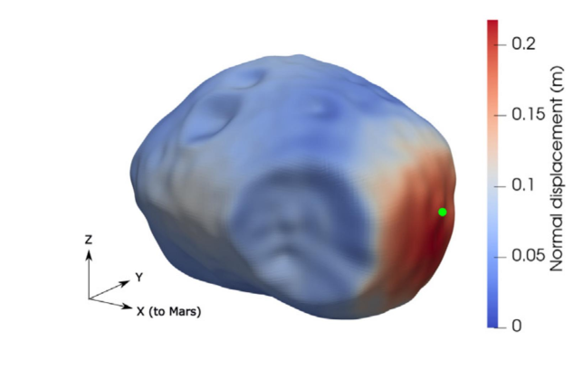
5.5 Moons of giant planets

The tidal response of the moons of the giant planets became a topic of great interest after it was recognised that tidal dissipation in these moons’ interiors can be a significant source of heat (Cassen et al., 1979) (Figures 15 and 17). Like for other bodies addressed in Section 5, tidal forcing also plays a role in the evolution of the moon dynamical properties (spin, orbit), and tidal stress can drive tectonic activity on some of the moons. The most famous examples are Enceladus’s Tiger stripes and associated jet activity whose temporal variability is correlated with tidal forcing (Hedman et al., 2013). Europa is another example, whose regional-scale ridges and cycloidal ridges have been produced from continuous forcing driving fatigue and eventual fracturing of surface material (Rhoden et al., 2021). In this section, we review the knowledge on the largest moons of giant planets with particular attention to the tidal dissipation as a heat source for different phenomenon within the interior of the moons. In Section 5.6, we will concentrate on the surface geological features as a result of tidal activity.

Figure 15: Thermal heat budget for outer Solar System satellites, broken down in terms of radiogenic heating, and eccentricity and obliquity tides applied to the ocean and solid layers of the moons. This example assumes $k_{2}=3/2$. From Chen et al. (2014), permission pending.

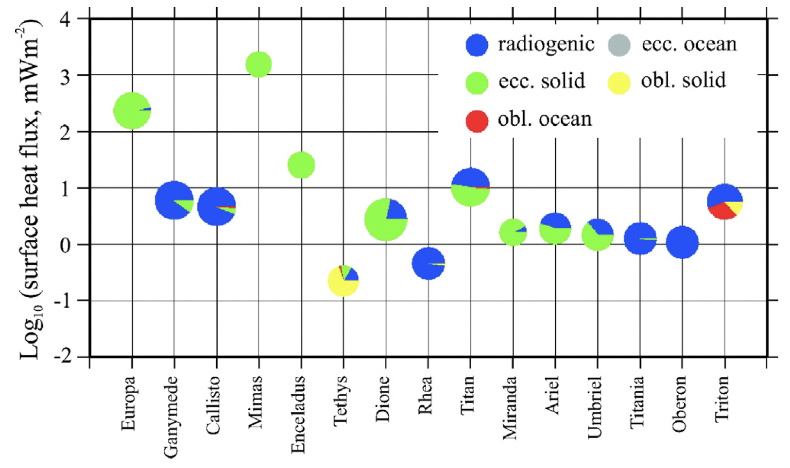
Io is the most volcanically active object in the Solar system (Figure 16). Its tidal heating power is estimated between 65 and 125 TW (Lainey et al., 2009). Io’s potential for significant tidal heating was suspected (Peale et al., 1979) Even before Voyager 1 flew through the Jovian system. Despite several observations by missions and a sustained ground-based observation program, we still lack a full understanding of the mechanisms driving tidal heating in Io, and especially what this activity tells us about Io’s deep interior. Galileo magnetic field observations hint that the moon could contain a deep magma layer, although its origin is debated (see Van Hoolst et al. (2020) for discussion). Using measurements of volcanic activity as a proxy for surface heat flow, based on spacecraft datasets covering several decades, Rathbun et al. (2018) found lower activity in the equatorial region at the anti-Jovian and sub-Jovian points. They also identified peak heat flow at mid-latitudes and a fourfold symmetry of upwellings distribution in longitude. The distribution of high dissipation regions inside Io is very dependent on the localization of the dissipation: in the asthenosphere or the underlying mantle (see Figure 16 for a definition of these terms). Kervazo et al. (2022) demonstrated that the distribution of tidal heating between the mantle and the asthenosphere is very sensitive to the melt fraction in the asthenosphere. If this fraction is low (high), then dissipation may occur preferentially in the mantle (asthenosphere). This behavior is characterized by a drastic difference in the surface expression of tidal heating. Rathbun et al. (2018) suggested that their observations were consistent with the tidal heating model by Tackley et al. (2001) where large-scale convective pattern dominates the distribution of tidal heating, and smaller-scale asthenospheric instabilities spread out the surface heat flux. On the other hand, the presence of a deep magma ocean would shift the distribution of activity peaks by 30 deg. (Tyler et al., 2015) in comparison to the Rathbun et al. observations. Kervazo et al. (2022) predicted that the tidal Love numbers $h_{2}$ and especially $l_{2}$ are more sensitive than $k_{2}$ to the melt distribution and would allow distinguishing between a mantle-dominated and asthenosphere-dominated regimes. This difference is amplified by bulk heat production. Furthermore, Van Hoolst et al. (2020) found that the diurnal libration amplitude of Io is several times larger if Io has a magma ocean compared to a partially molten asthenosphere. These authors predicted that the libration amplitude could be greater than 1 km in the former case. Upcoming missions, such as JUICE (JUpiter ICy moons Explorer, to be launched in 2023) and potential observations by Juno (two close Io flybys in 2023 and 2024) might be able to shed more light on Io’s behavior.

The contribution of tidal heating to promoting global ice melting and then preserving a deep ocean over long-time scales is not well quantified in most bodies. Tidal forcing likely played a major role in the formation of a deep ocean in Enceladus, as the moon’s small size and limited production from radioisotope decay would prevent global scale melting. It has been suggested that Saturn’s inner moons (within Titan’s orbit) formed in Saturn’s rings and evolved outward as a result of tidal interactions with the rings and the planet (Charnoz et al., 2011). The moons could form from heterogeneous accretion of porous ice on silicate chards embedded in the rings. Then, they would exit the rings in sequence, with Rhea being the oldest moon and Mimas the youngest. This scenario could explain why the moons’ densities do not follow a monotonic increase with distance to the planet, as would be expected if they formed in a circumplanetary disk. If the moons emerged from the ring, then they could have been subject to significant heating in their early history since they formed closer to the planet and their eccentricities were potentially excited by collisions with other emerging moons (Charnoz et al., 2011). However, an end-to-end evolution scenarios of these bodies has not been investigated yet.

Figure 16: Cross-sections of the Galilean moons’ interior structure based on the gravity data from Galileo mission. Various phases of ice and ice-silicate mixtures and metallic parts are present within the moons. This necessitates appropriate interior modeling of these objects.

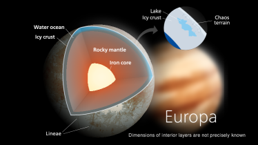
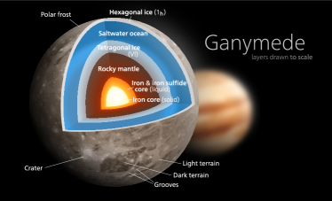
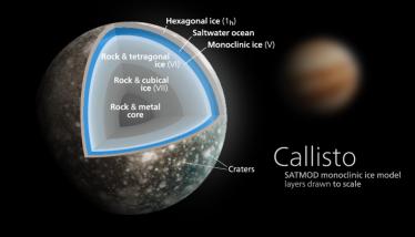
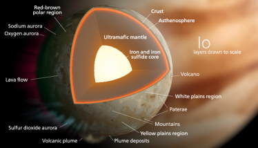
The feedback between tidal dissipation and orbital evolution can lead to a cycle of internal melting and freezing with geological expressions such as partial resurfacing (see for example Hussmann and Spohn (2004) for Europa). Resonance crossing, when the orbital periods of two bodies becomes near-commensurate as a result of orbital migration, can trigger significant heating. For example, Uranus’s moons Miranda and Ariel have recorded in their geology evidence of high heat flow, tens of mW/m² vs. < 0.01 mW/m² for their current eccentricities (e.g., Beddingfield et al. (2015), Beddingfield and Cartwright (2021)). This high heat flow has been attributed to the crossing of resonances: a possible 5:3 resonance between Ariel and Umbriel and a 3:1 resonance between Miranda and Ariel. In resonances, the eccentricities (and sometimes the inclinations) of moons are excited.

Figure 17: Icy satellite rock mass fractions and first-order tidal heating power (assuming $k_{2}/Q=1$) with schematic representation of observed surface geology, which can reflect the potential for endogenic activity and the (past or current) presence of a subsurface ocean. The dashed line indicates current-day heating due to natural decay of radioisotopes in the rock. Based on Castillo-Rogez and Lunine (2012), with updated information on Charon from New Horizons data.

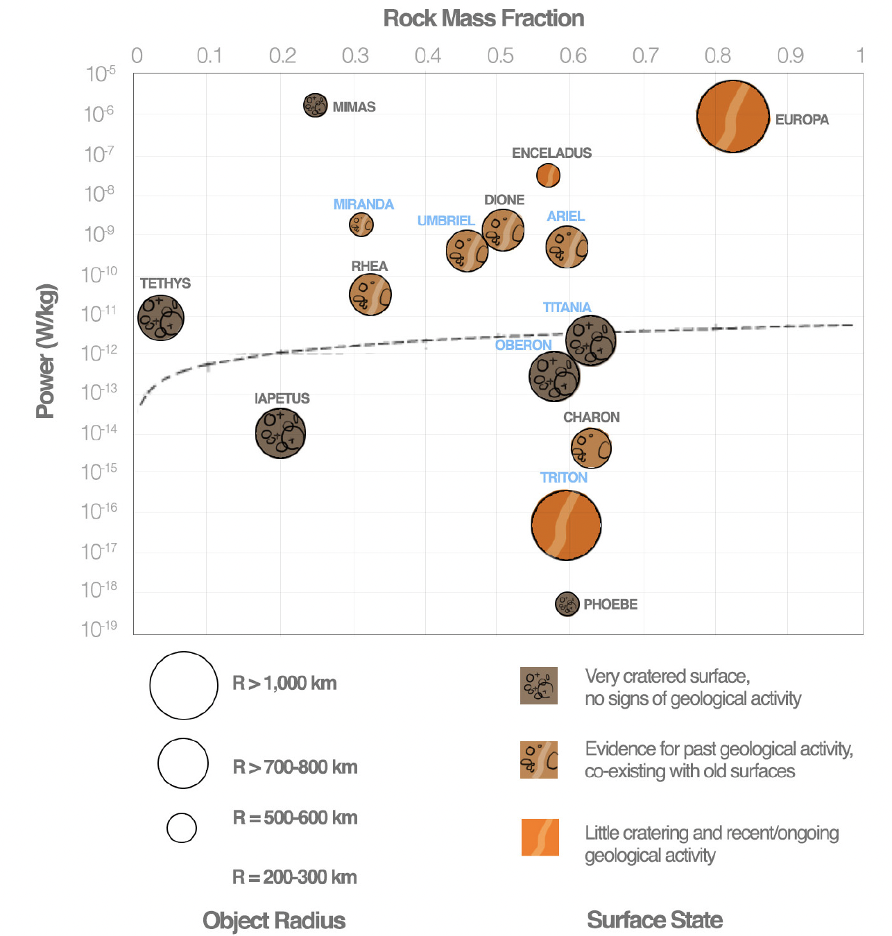
It was recently suggested that tidal forcing could also drive oceanic current (Rossby-Haurwitz waves) with potentially important implications (Tyler, 2014). Whether or not this mechanism could represent a long-term heat source in some of the moons is uncertain at this time. Chen et al. (2014) found that obliquity-driven tides in moon oceans could yield power of the same order as radioactive decay heat (Figure 15). In the case of Neptune’s moon Triton, obliquity-driven tides might be the key to the moon’s geologically young surface and ongoing activity (e.g., Nimmo and Spencer (2015); Hansen et al. (2021)). Indeed, obliquity-driven tides in the ocean could generate up to 300 GW (Nimmo and Spencer, 2015), which is about five times greater than the power produced from radioisotope decay heat and six orders of magnitude greater than power generated from eccentricity tides. Recent work by Matsuyama et al. (2018) focusing on the coupling of the ocean to the ice shell showed that the outer ice shell tends to damp ocean tides and decrease their contribution to tidal heating. These authors highlighted that the obliquity phase lag is sensitive to ocean thickness and is large (18 deg. for a reference ocean thickness of 100 km below a 10-km thick shell) and may be measured by a future mission (e.g., Europa Clipper). Furthermore, Hay et al. (2022) computed that at high frequencies, tidal deformation driven by interactions among moons could be amplified by ocean dynamics. However, the amplitude of this high frequency tidal response is too small to be detectable via spacecraft.

In their work on the endogenic activity near the Enceladean south pole, Howett et al. (2011) proposed that the outgoing energy flow associated with the tiger stripes geysers is of the order of $16$ GW. Many explanations have been suggested for this high power, most of which have been summarized by Nimmo et al. (2018). In a rough calculation, Efroimsky (2018) modeled Enceladus with a homogeneous sphere composed of a Maxwell material, and calculated the amount of tidal power dissipated in it, with an input from forced libration in longitude taken into account. The so-obtained formula established a direct link between the power and the mean viscosity of Enceladus. The subsequent insertion of the measured value of heat outflow resulted in the value of the mean viscosity, which exactly coincided with the viscosity of ice near melting point. This simple estimate demonstrated that tides are sufficient to explain Enceladus’s high heat power.

Among the recent developments in our understanding of the tidal dissipation in icy moons are more elaborate models, e.g. one permitting for water circulation in porous cores (fractured but solid, or rubble piles) (Choblet et al., 2017). Likely active in mid-sized moons (<1000 km radius, Neveu and Rhoden (2019b)), this mechanism may be contributing to Enceladus’s heat production, along with the significant dissipation in the ice shell and, potentially, in the ocean. Further insights in the surface geological activity of Enceladus will be provided in Section 5.6.

The implications of tidal interactions between a moon and planet depend on the $k_{2}/Q$ of the planet. For a long time, these parameters were poorly known. Indeed, tidal friction within Saturn causes its moons to migrate outwards, and tidal evolution determines their current position. Based on astrometric observations obtained with the Cassini spacecraft, Lainey et al. (2017) showed that dissipation in Saturn is at least one order of magnitude larger ($k_{2}/Q=(1.59\pm 0.74)\times 10^{-4}$) than assumed in past theoretical studies. These authors also identified that Saturn’s tidal response might be frequency dependent by comparison between the tidal evolution of the midsized moons.

Disentangling the relationships between internal evolution and dynamical evolution offers prospects to explain the origin of the Saturnian moons (and maybe the Uranian moons when more observation becomes available). If the moons formed in Saturn’s rings then, the evolution to their current locations can set constraints on Saturn’s $k_{2}/Q$. On the other hand, if the moons formed near their current locations, then Saturn’s $Q$ needs to be high (about 80,000, Ćuk et al. (2016)), which does not appear consistent with Enceladus’s high dissipation. Additional observations with Cassini lead Lainey et al. (2020) to demonstrate that Titan is migrating away from Saturn faster than previously envisioned, leading to an estimate of Saturn’s $Q$ of about 100. These authors also inferred that Titan could have formed much closer to Saturn than its current location. Fuller et al. (2016) introduced the resonance locking theory between moons and internal oscillation modes of the planet as a way to address a number of observations in the Saturnian and Galilean systems. Resonance locking opposes the constant $Q$ assumption used for decades. Fuller et al. (2016) inferred that this effect is the dominant driver of tidal dissipation in these systems and suggested that the resonance locking theory allows the large heating rate of Enceladus to be achieved in an equilibrium eccentricity configuration. Nimmo et al. (2018) pointed out that the astrometric observations at the basis of the resonance locking scenarios and follow on studies carry large uncertainties and only a narrow set of Saturn’s $k_{2}/Q$ allows the onset of resonances. These authors further noted that the impact of resonances on the internal evolution of satellites, especially under increase dissipation peak when they cross mean motion resonances is not accounted for. Tidal dissipation within the moons could counteract Saturn’s influence by decreasing eccentricity and semi-major axis.

The thermal and orbital evolution of icy moons are coupled via the thermomechanical properties of their materials (see Section 3.2). There is evidence that Saturn’s midsized moons have been very dissipative in their past, expressed in the geology (e.g., flexure relaxation, crater morphologies). This has been ascribed to resonance crossing (e.g., Chen and Nimmo (2008) for Tethys). Convective regions (e.g., convective plumes) can also be areas of enhanced tidal heating. Sotin et al. (2002) suggested that tidal forcing can drive the formation of diapirs that may be involved in the formation of lenticulae and chaos regions at the surface of Europa. Tobie et al. (2003) further explored this idea and predict a heat flow of 35 to 40 mW/m^-2 constant across Europa’s surface. Further details on the surface geological activity on Europa will be provided in Section 5.6. In the case of Titan, Tobie et al. (2005a) found that a few percent of ammonia in the ocean is needed to limit the dissipation in the shell (by decreasing the basal temperature of the shell) and preserve a high eccentricity (0.009), although alternative models have been suggested to explain this high eccentricity (e.g., Ćuk et al. (2016)) More work is needed to establish an end-to-end model of the evolution of the Saturnian moon system as a whole.

A recent analysis of the tidal evolution of the Uranian moons following their crossing mean motion resonances has led to constraints on their ${Q}/{k_{2}}$ (Ćuk et al., 2020). It ranges from 10⁴ for Oberon (the farthest from Uranus) to 10⁶ for Miranda (closest moon), suggesting a wide range of internal properties across the Uranian moons system. Considering the moon’s $k_{2}$ may range from 10^-3 to 10^-2 (Hussmann et al., 2006), we infer dissipation factors in excess of 1000 in Miranda, and potentially also Oberon, suggesting that the moons are not dissipative at present and may be near frozen. Interestingly, the Uranian moon system is not in resonances at present.

Actual constraints on the tidal parameters of icy moons are few. Multiple flybys of Saturn’s moon Titan by the Cassini orbiter led to the inference of $k_{2}=0.637\pm 0.0220$ (Iess et al. 2014). This high value has been interpreted as evidence for a high density of the ocean, of the order of 1200 kg/m³ (e.g., Mitri et al. (2014); Baland et al. (2014)). This high density points to a high content in salt (Baland et al., 2014) that cannot be uniquely explained by cosmochemical abundances but also involves a contribution of non-water ice volatiles (e.g., CO₂, NH₃) to oceanic solutes (e.g., bi/carbonate and ammonium ions. This high density may also reflect a large abundance of clathrate hydrate, such as CO₂ hydrates, whose density is about 1100 kg/m³ (Boström et al., 2021).

Despite the critical contribution of tidal stressing to the heat budgets of large icy moons, models miss input parameters that have been obtained in conditions relevant to these objects. By lack of knowledge on the internal properties of small moons (<1000 km radius), many studies assume a dissipation factor Q = 100 for these bodies, as well as a tidal Love number based on a homogeneous interior. However, as shown above, dissipation is a function of the material frequency-dependent mechanical response, which itself depends on temperature and the history of the material. Dissipation in porous interiors (e.g., near Earth asteroids), mixtures of water ice, salts, and clathrates, that may be relevant to Europa or Titan, for example, are scarce. Tidal stresses at icy moons have a wide range of amplitudes that invoke different response mechanisms. Reproducing low stress and long forcing periods in laboratory is challenging and most cyclic forcing measurements have been obtained at frequencies greater than 10^-4 Hz. Future experimental work should aim to retire some of these knowledge gaps that prevent more high-fidelity modeling of the moon internal evolution.

The Europa Clipper mission’s gravity measurement is projected to yield Europa’s tidal Love number $k_{2}$ with an accuracy of 0.015 (1-$\sigma$) (Mazarico et al., 2021). The combination of ground penetrating radar and imaging will yield $h_{2}$ (Steinbrügge et al., 2021) but the predicted accuracy is still a work in progress. The JUICE mission is also planning to obtain these parameters at Ganymede, in particular $k_{2}$ with an accuracy of 10^-4 (e.g., Cappuccio et al., 2020).

5.6 Tidal signature on planetary surfaces

This review mainly addresses deciphering the interior structure based on measurements of tidal response presented in the form of Love numbers as well as the reciprocal effect of tidal heating and interior properties in the planetary bodies. However, it is important to mention how surface geological features as a result of tidal activities can also be used to constrain both the present-day interior and thermal-orbital evolution of the planetary bodies through their relationship to tidal stress and tidal evolution.

Hence, we dedicate this section to overview the effect of surface features as a result of tidal activities and their interpretations for the interior in different planetary bodies, particularly the icy moons. While, a more detailed review of the tidal signatures on the surface of the planets would need a dedicated study, here we only provide a summary of the most important findings on the interior as a result of studying the surface of the icy moons.

The extent to which the surface of a moon will be affected by tidal stress not only depends on the orbital elements such as eccentricity, obliquity, and the proximity to the parent planet, but also to the responsiveness of the of the interior of the body to tidal deformation, which in turn is strongly affected by the presence or absence of an ocean, the rheology of the interior, and the amount of internal heat being generated within the moon (e.g., Greenberg et al., 1998; Jara-Orué and Vermeersen, 2011; Rhoden and Walker, 2022). Thus, geologic features on the planetary objects can provide insight as to their interior structures and thermal states. For example, the presence, absence, and style of tectonic activity can be diagnostic of a moon’s thermal history (e.g., Rhoden et al., 2020). Similarly, the presence of eruptions, whether in the form of surface flows or geysers, can provide insight into the cooling history of a moon and the composition of its ocean (e.g., Rudolph et al., 2022). Lastly, indicators of past heat flows, through changes to crater morphology, can constrain the overall thermal history of a moon (e.g., Bland et al., 2012)

Although still an area of active study, some consistent links have been identified between certain geologic features and the inferred thermal-orbital history or interior structure of a moon. We begin with tectonics. The two icy satellites with extensive canyon systems, Tethys at Saturn and Charon at Pluto, both have negligible present-day orbital eccentricities, with reason to expect that they underwent rapid despinning and circularization (Peale, 1999; Neveu and Rhoden, 2019a; Cheng et al., 2014). Neither moon is expected to have an ocean today due to a lack of potential heat sources, although observational constraints on Tethys’s interior are quite limited (Castillo-Rogez et al., 2018). Tethys and Charon both have globally-distributed, but overall sparse, fracture systems that appear unrelated to either the canyons or tidal stress patterns (Castillo-Rogez et al., 2018; Rhoden et al., 2020). Their origin is currently unknown. As described in Rhoden et al. (2020), the best explanation of the formation of the canyons on Tethys and Charon is that both moons began with high eccentricity orbits that generated oceans through tidal dissipation. As a result, the orbits circularized, and the lack of tidal heating led the oceans to freeze out. As oceans freeze, the thermal stresses and the increase in volume of the newly accreted ice at the base of the shell can create radial fractures within an ice shell (Rudolph and Manga, 2009; Rudolph et al., 2022). Hence, the cooling and freezing of the interior may have produced the initial fractures that developed into canyons through continued thickening of the ice shell. The lack of fractures associated with tidal stress patterns comes from the fact that circularization occurred before the ocean froze, so there were no tidal stresses available Rhoden et al. (2020). Thus, we can hypothesize that canyon systems are indicative of a past ocean that has completely frozen out.

One important difference between Charon and Tethys is that only Charon shows evidence of cryovolcanism. A potential explanation for this difference is that fractures formed through ocean freezing were able to crack through the entire ice shell at Charon but not at Tethys, perhaps because the Tethys’s interior did not warm up as much as Charon’s, and the ice shell was correspondingly thicker. Given that Tethys is approximately 94% ice (Castillo-Rogez et al., 2018), it may have had too little rocky material to provide sufficient radiogenic heating to reach a similar level of melting as Charon, or it may have begun with a lower eccentricity that resulted in less tidal heating. The presence of ammonia within Charon’s interior, as explored by Bagheri et al. (2022) could also facilitate eruptions and would likely be absent or less abundant within Tethys. In any case, comparing the geology of these two moons provides insight into differences in the thermal evolution of their interiors. On the opposite end of the tectonic spectrum are moons with oceans thicker than their overlying ice shells. Europa at Jupiter and Enceladus at Saturn (e.g., Nimmo and Pappalardo, 2016) are the two “confirmed" ocean worlds of this type. Both of these moons execute eccentric orbits while orbiting close to their parent planet; their subsurface oceans and warm ice shells allow for significant tidal deformation and stress in the overlying cold ice. Europa’s surface is pervasively, and globally, fractured, and the fractures vary in their surface expression from linear to wavy to cycloidal (e.g., Kattenhorn and Hurford, 2009) (See Figure 16). The shapes of cycloids, linked arcs that can span 100s of km, track the spatial and temporal changes in tidal stress throughout Europa’s orbit (Greenberg et al., 1998; Hoppa et al., 2001; Rhoden et al., 2010, 2021). Fits to both individual cycloid shapes and the overall distribution of cycloids greatly improved when the effects of a small obliquity were added to the tidal stress model, illustrating the powerful link between the orbit, interior, and surface geology. Europa also displays strike-slip offsets along many fractures, long parallel bands formed from extension, and irregularly-shaped bands formed from compression/subsumption (see reviews by Kattenhorn and Hurford (2009); Prockter and Patterson (2009). Many strike-slip offsets have been linked to tides (e.g., Rhoden et al., 2012), whereas band formation appears to result from large-scale plate motion (e.g., Kattenhorn and Prockter, 2014), which may be governed by different processes.

Enceladus displays tectonic features that are morphologically-similar to those at Europa, but Enceladus’s tectonism is regional, with activity concentrated near the south pole (Spencer et al., 2006; Patthoff and Kattenhorn, 2011; Crow-Willard and Pappalardo, 2015). Also, Enceladus lacks cycloids, strike-slip offsets along fractures, and bands of any kind. The four, roughly parallel fractures within the south polar terrain (dubbed “Tiger Stripes") have orientations consistent with eccentricity-driven tidal stresses (Rhoden et al., 2020), and the geyser-like eruptions emanating from the Tiger Stripes vary in output on a diurnal timescale, suggesting a link to tides (Nimmo et al., 2007; Hurford et al., 2007; Hedman et al., 2013). The ice shell thickness on Enceladus appears to vary considerably with location (e.g., Thomas et al., 2016; Beuthe et al., 2016; Čadek et al., 2019); the shell is thinnest at the south pole and thickest along the equator. In a heterogeneous ice shell, tidal stresses are enhanced at thin zones (Beuthe, 2019). Thus, the extent of tectonic activity may well be an indicator of ice shell thickness, with older tectonized regions representing past thin zones. This interpretation would suggest that, as at Europa, multiple generations of crisscrossing, ridge-flanked fractures are indicative of relatively thin ice shells and concentrated tidal stress. Between these two extremes, there are a variety of heavily cratered moons with varying levels of tectonic activity, including Ganymede at Jupiter and Dione at Saturn. Both moons are thought to have thin oceans beneath much thicker ice shells, and they both orbit far enough from their parent planet to have reduced tidal heating and stress, which may be the reason for their limited geologic activity. Callisto at Jupiter and Rhea at Saturn orbit even farther away and both are heavily cratered with little other geologic activity. There is some evidence to suggest a deep, thin ocean within Callisto (Khurana et al., 1998), so it is possible that even heavily cratered worlds can have oceans; much less is known about the interior structure of Rhea (Tortora et al., 2016). Taken together, it seems that there is a correlation between ocean thickness, relative to total hydrosphere thickness, and the extent of tectonic activity.

One curious outlier is Saturn’s smallest and innermost regular satellite, Mimas. With a higher eccentricity than its exterior neighbor, Enceladus, we might expect Mimas to be even more geologically active, akin to Io at Jupiter. However, Mimas is heavily cratered with few tectonic features and no evidence of volcanic activity. And yet, model fits to Cassini measurements of Mimas’s physical librations indicate that Mimas is likely an ocean-bearing world and require that Mimas is differentiated into a rocky interior and outer hydrosphere (Tajeddine et al., 2014; Noyelles, 2017; Caudal, 2017). If Mimas does, indeed, have a subsurface ocean today, it may be a young ocean world, such that its surface has not had time to develop the characteristics features observed on moons such as Europa and Enceladus (see also Rhoden and Walker (2022)). In addition to tectonic and volcanic activity, craters can be quite diagnostic of the interior structure and heating history of a moon. Most obviously, the morphology of the initial impact can be used to constrain the thickness of the outmost layer of the moon. For example, some craters have clearly cracked through Europa’s entire ice shell to the ocean beneath (see Schenk and Turtle (2021), for an overview), whereas several of the mid-sized moons of Saturn have large (100s of km) impact basins that show no evidence of a subsurface ocean. However, tidal dissipation within an icy satellite can also have a more subtle, but still diagnostic, effect on craters.

As heat is transferred from the interior of a moon to the surface, it can modify the shapes of existing craters, creating flatter floors and overall subdued morphologies. The process, called crater relaxation, records the magnitude and longevity of heat flow through the ice shell. Crater relaxation on Enceladus, Tethys, Dione, and Rhea all indicate past episodes of higher heat flows (Bland et al., 2012; White et al., 2013, 2017). Even Enceladus, which has high present-day heat flows, would require a past epoch of considerably more dissipation to explain the observed crater shapes (Bland et al., 2012). For the other moons, to achieve the observed levels of relaxation would imply temperatures above the melting temperature of water ice, suggesting oceans within their surface ages. In contrast, Mimas’s craters show no evidence of relaxation to within the observation limit imposed by image coverage. In that case, crater shapes provide an upper limit on the extent of tidal dissipation that could have taken place within Mimas. In all of these cases, it is the link between interiors, tidal dissipation, and surface geology that allows these features to provide additional insight as to the thermal-orbital evolution of the moons and their past and present interior structures.

6 Summary and conclusions

In this paper, we have attempted to provide an overview of the past, present, and future use of tides as a means of procuring information on the interior structure of planets and moons from orbiting and landed spacecraft. Since tidal response measurements play an inordinate role in understanding the interiors of rocky and icy planetary bodies, we provided a detailed outline of the fundamental concepts connected to modeling the tidal response, including the viscoelastic behaviour of planetary materials, and how the tides couple to the thermal structure within the planetary body to determine its subsequent orbital evolution. We also provided an overview of the surface geological features on icy moons as a result of tidal activity with interpretations for their interior structure and evolution.

This is also of fundamental importance for proper modeling and understanding of the evolution of extra-Solar planetary bodies that ultimately determines their astrobiological potential. In connection herewith are the latest extensions of modern tidal theory (Makarov and Efroimsky, 2013), including tidal evolution formulae that allow for the consideration of higher-order eccentricity functions required for accurate modeling of the evolution of planetary systems in and out of e.g., spin-orbit resonances, non-synchronous rotation, and mean motion resonances (Renaud et al., 2021; Bagheri et al., 2021). For exoplanets trapped in a higher-order spin-orbit resonance for an extended amount of time, for example, important climate variations could ensue as a result of a new Solar configuration (Del Genio et al., 2019) and thus the potential for life to develop. We provided an overview of the current state of investigation of the rocky bodies of our Solar system, including Mercury, Venus, the Moon, and Mars, and the icy moons of the giant planets from the point of view of tides that will invariably remain, relative to the more involved deployment of surface instrumentation, the most prominent means of inferring knowledge on the interior of the planets and satellites. The ongoing development of more refined tidal models, in combination with further experimental studies of the viscoelastic properties of planetary materials, and advances in geophysical models through continued analysis of geodetic and other large-scale measurements (e.g., InSight and LLR), promise new insights into the inner structure of terrestrial planets and moons of the Solar system.

7 Acknowledgments

We acknowledge informative discussions with Ian Jackson and Ulrich Faul on material viscoelasticity, and with Valeri Makarov on tides. A.B. was supported by a grant from the Swiss National Science Foundation (project 172508). J.C.’s contribution was developed at the Jet Propulsion Laboratory, California Institute of Technology, under contract with the National Aeronautics and Space Administration. M.W. and A.C.P. gratefully acknowledge the financial support and endorsement from the DLR Management Board Young Research Group Leader Program and the Executive Board Member for Space Research and Technology. The artistic views of the Moon and the Saturnian moons are taken or modified from https://commons.wikimedia.org/wiki/User:Kelvin13.

References

- Al-Attar and Tromp (2013) D. Al-Attar and J. Tromp. Sensitivity kernels for viscoelastic loading based on adjoint methods. Geophysical Journal International, 196(1):34–77, 2013.
- Alterman et al. (1959) Z. Alterman, H. Jarosch, and C. L. Pekeris. Oscillations of the Earth. Proceedings of the Royal Society of London Series A, 252(1268):80–95, Aug. 1959. 10.1098/rspa.1959.0138.
- Anderson and O’Connell (1967) D. L. Anderson and R. O’Connell. Viscosity of the Earth. Geophysical Journal International, 14(1-4):287–295, 1967.
- Anderson and Smrekar (2006) F. S. Anderson and S. E. Smrekar. Global mapping of crustal and lithospheric thickness on Venus. Journal of Geophysical Research: Planets, 111(E8), 2006.
- Anderson et al. (1987) J. D. Anderson, G. Colombo, P. B. Esposito, E. L. Lau, and G. B. Trager. The mass, gravity Field, and ephemeris of Mercury. Icarus, 71:337–349, 1987. 10.1016/0019-1035(87)90033-9.
- Andrade (1910) E. N. D. C. Andrade. On the viscous flow in metals, and allied phenomena. Proceedings of the Royal Society of London. Series A, Containing Papers of a Mathematical and Physical Character, 84(567):1–12, 1910.
- Arakawa et al. (2021) S. Arakawa, R. Hyodo, D. Shoji, and H. Genda. Tidal evolution of the eccentric moon around dwarf planet (225088) Gonggong. The Astronomical Journal, 162(6):226, 2021.
- Armann and Tackley (2012) M. Armann and P. J. Tackley. Simulating the thermochemical magmatic and tectonic evolution of Venus’s mantle and lithosphere: Two-dimensional models. Journal of Geophysical Research Planets, 117(E12):E12003, Dec. 2012. 10.1029/2012JE004231.
- Asphaug et al. (1998) E. Asphaug, S. J. Ostro, R. Hudson, D. J. Scheeres, and W. Benz. Disruption of kilometre-sized asteroids by energetic collisions. Nature, 393(6684):437, 1998.
- Auclair-Desrotour et al. (2017) P. Auclair-Desrotour, J. Laskar, and S. Mathis. Atmospheric tides in Earth-like planets. Astronomy and Astrophysics, 603:A107, July 2017. 10.1051/0004-6361/201628252.
- Bagdassarov and Dingwell (1993) N. S. Bagdassarov and D. B. Dingwell. Frequency dependent rheology of vesicular rhyolite. Journal of Geophysical Research: Solid Earth, 98(B4):6477–6487, Apr. 1993. 10.1029/92JB02690.
- Bagheri et al. (2015) A. Bagheri, S. Greenhalgh, A. Khojasteh, and M. Rahimian. Dispersion of Rayleigh, Scholte, Stoneley and Love waves in a model consisting of a liquid layer overlying a two-layer transversely isotropic solid medium. Geophysical Journal International, 203(1):195–212, 2015.
- Bagheri et al. (2019) A. Bagheri, A. Khan, D. Al-Attar, O. Crawford, and D. Giardini. Tidal response of Mars constrained from laboratory-based viscoelastic dissipation models and geophysical data. Journal of Geophysical Research planets, 2019.
- Bagheri et al. (2021) A. Bagheri, A. Khan, M. Efroimsky, M. Kruglyakov, and D. Giardini. Dynamical evidence for Phobos and Deimos as remnants of a disrupted common progenitor. Nature Astronomy, pages 1–5, 2021.
- Bagheri et al. (2022) A. Bagheri, A. Khan, F. Deschamps, H. Samuel, M. Kruglyakov, and D. Giardini. The tidal-thermal evolution of the Pluto–Charon system. Icarus, 2022.
- Baland et al. (2014) R.-M. Baland, G. Tobie, A. Lefèvre, and T. Van Hoolst. Titan’s internal structure inferred from its gravity field, shape, and rotation state. Icarus, 237:29–41, 2014.
- Banerdt et al. (2020) W. B. Banerdt, S. E. Smrekar, D. Banfield, D. Giardini, M. Golombek, C. L. Johnson, P. Lognonné, A. Spiga, T. Spohn, C. Perrin, et al. Initial results from the InSight mission on Mars. Nature Geoscience, pages 1–7, 2020.
- Basaltic Volcanism Study Project (1981) Basaltic Volcanism Study Project. Basaltic Volcanism on the Terrestrial Planets. Pergamon Press, New York, 1981.
- Beddingfield et al. (2015) C. Beddingfield, D. Burr, and J. Emery. Fault geometries on Uranus’ satellite Miranda: Implications for internal structure and heat flow. Icarus, 247:35–52, 2015.
- Beddingfield and Cartwright (2021) C. B. Beddingfield and R. J. Cartwright. A lobate feature adjacent to a double ridge on Ariel: Formed by cryovolcanism or mass wasting? Icarus, 367:114583, 2021.
- Benjamin et al. (2006) D. Benjamin, J. Wahr, R. D. Ray, G. D. Egbert, and S. D. Desai. Constraints on mantle anelasticity from geodetic observations, and implications for the J2 anomaly. Geophysical Journal International, 165:3–16, Apr. 2006. 10.1111/j.1365-246X.2006.02915.x.
- Benkhoff et al. (2010) J. Benkhoff, J. van Casteren, H. Hayakawa, M. Fujimoto, H. Laakso, M. Novara, P. Ferri, H. R. Middleton, and R. Ziethe. BepiColombo - Comprehensive exploration of Mercury: Mission overview and science goals. Planetary and Space Science, 58:2–20, Jan. 2010. doi:10.1016/j.pss.2009.09.020.
- Bertone et al. (2021) S. Bertone, E. Mazarico, M. K. Barker, S. Goossens, T. J. Sabaka, G. A. Neumann, and D. E. Smith. Deriving Mercury geodetic parameters with altimetric crossovers from the Mercury Laser Altimeter (MLA). Journal of Geophysical Research: Planets, 126(4):e06683, Apr. 2021. 10.1029/2020JE006683.
- Beuthe (2013) M. Beuthe. Spatial patterns of tidal heating. Icarus, 223(1):308–329, 2013. 10.1016/j.Icarus.2012.11.020.
- Beuthe (2019) M. Beuthe. Enceladus’s crust as a non-uniform thin shell: II tidal dissipation. Icarus, 332:66–91, 2019.
- Beuthe et al. (2016) M. Beuthe, A. Rivoldini, and A. Trinh. Enceladus’s and Dione’s floating ice shells supported by minimum stress isostasy. Geophysical Research Letters, 43(19):10–088, 2016.
- Bierson et al. (2020) C. J. Bierson, F. Nimmo, and S. A. Stern. Evidence for a hot start and early ocean formation on Pluto. Nature Geoscience, 13(7):468–472, 2020.
- Bills et al. (2005) B. G. Bills, G. A. Neumann, D. E. Smith, and M. T. Zuber. Improved estimate of tidal dissipation within Mars from MOLA observations of the shadow of Phobos. Journal of Geophysical Research Planets, 110:E07004, July 2005. 10.1029/2004JE002376.
- Biot (1954) M. A. Biot. Theory of stress-strain relations in anisotropic viscoelasticity and relaxation phenomena. Journal of Applied Physics, 25(11):1385–1391, 1954.
- Bland et al. (2012) M. T. Bland, K. N. Singer, W. B. McKinnon, and P. M. Schenk. Enceladus’ extreme heat flux as revealed by its relaxed craters. Geophysical Research Letters, 39(17), 2012.
- Bolmont et al. (2020) E. Bolmont, S. N. Breton, G. Tobie, C. Dumoulin, S. Mathis, and O. Grasset. Solid tidal friction in multi-layer planets: Application to Earth, Venus, a Super Earth and the TRAPPIST-1 planets. Potential approximation of a multi-layer planet as a homogeneous body. Astronomy and Astrophysics, 644:A165, Dec. 2020. 10.1051/0004-6361/202038204.
- Borrelli et al. (2021) M. E. Borrelli, J. G. O’Rourke, S. E. Smrekar, and C. M. Ostberg. A global survey of lithospheric flexure at steep-sided domical volcanoes on Venus reveals intermediate elastic thicknesses. Journal of Geophysical Research: Planets, 126(7):e2020JE006756, 2021.
- Boström et al. (2021) M. Boström, V. Esteso, J. Fiedler, I. Brevik, S. Y. Buhmann, C. Persson, S. Carretero-Palacios, D. F. Parsons, and R. W. Corkery. Self-preserving ice layers on CO2 clathrate particles: Implications for Enceladus, Pluto, and similar ocean worlds. Astronomy & Astrophysics, 650:A54, 2021.
- Boué and Efroimsky (2019) G. Boué and M. Efroimsky. Tidal evolution of the Keplerian elements. Celestial Mechanics and Dynamical Astronomy., 131(7):30, 2019.
- Briaud (2022) Briaud. . submitted, 2022.
- Burgers (1935) J. Burgers. Mechanical considerations-model systems-phenomenological theories of relaxation and of viscosity. First report on viscosity and plasticity, 1, 1935.
- Běhounková et al. (2015) M. Běhounková, G. Tobie, O. Čadek, G. Choblet, C. Porco, and F. Nimmo. Timing of water plume eruptions on Enceladus explained by interior viscosity structure. Nature Geoscience, 8(8):601–604, Aug. 2015. 10.1038/ngeo2475.
- Čadek et al. (2019) O. Čadek, O. Souček, M. Běhounková, G. Choblet, G. Tobie, and J. Hron. Long-term stability of Enceladus’ uneven ice shell. Icarus, 319:476–484, 2019.
- Campagnola et al. (2018) S. Campagnola, C. H. Yam, Y. Tsuda, N. Ogawa, and Y. Kawakatsu. Mission analysis for the Martian Moons Explorer (MMX) mission. Acta Astronautica, 146:409–417, 2018.
- Canup and Asphaug (2001) R. M. Canup and E. Asphaug. Origin of the Moon in a giant impact near the end of the Earth’s formation. Nature, 412(6848):708–712, 2001.
- Cappuccio et al. (2020) P. Cappuccio, A. Hickey, D. Durante, M. Di Benedetto, L. Iess, F. De Marchi, C. Plainaki, A. Milillo, and A. Mura. Ganymede’s gravity, tides and rotational state from JUICE’s 3GM experiment simulation. Planetary and Space Science, 187:104902, 2020.
- Cartier et al. (2020) C. Cartier, O. Namur, L. R. Nittler, S. Z. Weider, E. Crapster-Pregont, A. Vorburger, E. A. Frank, and B. Charlier. No FeS layer in Mercury? Evidence from Ti/Al measured by MESSENGER. Earth and Planetary Science Letters, 534:116108, Mar. 2020. 10.1016/j.epsl.2020.116108.
- Cascioli et al. (2021) G. Cascioli, S. Hensley, F. De Marchi, D. Breuer, D. Durante, P. Racioppa, L. Iess, E. Mazarico, and S. E. Smrekar. The determination of the rotational state and interior structure of Venus with VERITAS. Planetary Science Journal, 2(6):220, Dec. 2021. 10.3847/PSJ/ac26c0.
- Cassen et al. (1979) P. Cassen, R. T. Reynolds, and S. Peale. Is there liquid water on Europa? Geophysical Research Letters, 6(9):731–734, 1979.
- Castillo-Rogez and Lunine (2012) J. Castillo-Rogez and J. Lunine. Small habitable worlds. Frontiers of astrobiology, pages 201–228, 2012.
- Castillo-Rogez et al. (2018) J. Castillo-Rogez, D. Hemingway, A. Rhoden, G. Tobie, and W. McKinnon. Origin and evolution of Saturn’s mid-sized moons. Enceladus and the Icy Moons of Saturn, page 285, 2018.
- Castillo-Rogez and Banerdt (2012) J. C. Castillo-Rogez and W. B. Banerdt. Impact of Anelasticity on Mars’ Dissipative Properties - Application to the InSight Mission. In The Mantle of Mars: Insights from Theory, Geophysics, High-Pressure Studies, and Meteorites, volume 1684 of LPI Contributions, page 4, Sept. 2012.
- Castillo-Rogez et al. (2011) J. C. Castillo-Rogez, M. Efroimsky, and V. Lainey. The tidal history of Iapetus: Spin dynamics in the light of a refined dissipation model. Journal of Geophysical Research (Planets), 116(E9):E09008, Sept. 2011. 10.1029/2010JE003664.
- Caudal (2017) G. Caudal. The damping of forced librations of triaxial satellites with eccentric orbits: Consequences on the dynamics of Mimas. Icarus, 286:280–288, 2017.
- Cavanaugh et al. (2007) J. F. Cavanaugh, J. C. Smith, X. Sun, A. E. Bartels, L. Ramos-Izquierdo, D. J. Krebs, J. F. McGarry, R. Trunzo, A. M. Novo-Gradac, J. L. Britt, J. Karsh, R. B. Katz, A. T. Lukemire, R. Szymkiewicz, D. L. Berry, J. P. Swinski, G. A. Neumann, M. T. Zuber, and D. E. Smith. The Mercury laser altimeter instrument for the MESSENGER mission. Space Science Reviews, 131(1-4):451–479, Aug. 2007. 10.1007/s11214-007-9273-4.
- Cébron et al. (2019) D. Cébron, R. Laguerre, J. Noir, and N. Schaeffer. Precessing spherical shells: flows, dissipation, dynamo and the lunar core. Geophysical Journal International, 219(Supplement_1):S34–S57, 2019.
- Chabé et al. (2020) J. Chabé, C. Courde, J.-m. Torre, S. Bouquillon, A. Bourgoin, M. Aimar, D. Albanese, B. Chauvineau, H. Mariey, G. Martinot-Lagarde, et al. Recent progress in lunar laser ranging at grasse laser ranging station. Earth and Space Science, 7(3):e2019EA000785, 2020.
- Chabot et al. (2014) N. L. Chabot, E. A. Wollack, R. L. Klima, and M. E. Minitti. Experimental constraints on Mercury’s core composition. Earth and Planetary Science Letters, 390:199–208, Mar. 2014. 10.1016/j.epsl.2014.01.004.
- Chapront-Touzé and Chapront (1988) M. Chapront-Touzé and J. Chapront. ELP 2000-85-A semi-analytical lunar ephemeris adequate for historical times. Astronomy and Astrophysics, 190:342–352, 1988.
- Chapront-Touzé and Chapront (1991) M. Chapront-Touzé and J. Chapront. Lunar tables and programs from 4000 B.C. to A.D. 8000. 1991.
- Charnoz et al. (2011) S. Charnoz, A. Crida, J. C. Castillo-Rogez, V. Lainey, L. Dones, Ö. Karatekin, G. Tobie, S. Mathis, C. Le Poncin-Lafitte, and J. Salmon. Accretion of Saturn’s mid-sized moons during the viscous spreading of young massive rings: Solving the paradox of silicate-poor rings versus silicate-rich moons. Icarus, 216(2):535–550, 2011.
- Chawla and Meyers (1999) K. K. Chawla and M. Meyers. Mechanical behavior of materials. Prentice Hall Upper Saddle River, 1999.
- Chen and Nimmo (2008) E. Chen and F. Nimmo. Implications from Ithaca Chasma for the thermal and orbital history of Tethys. Geophysical research letters, 35(19), 2008.
- Chen et al. (2014) E. Chen, F. Nimmo, and G. Glatzmaier. Tidal heating in icy satellite oceans. Icarus, 229:11–30, 2014.
- Cheng et al. (2014) W. Cheng, M. H. Lee, and S. Peale. Complete tidal evolution of pluto–charon. Icarus, 233:242–258, 2014.
- Choblet et al. (2017) G. Choblet, G. Tobie, C. Sotin, M. Běhounková, O. Čadek, F. Postberg, and O. Souček. Powering prolonged hydrothermal activity inside Enceladus. Nature Astronomy, 1(12):841, 2017.
- Churkin (1998) V. Churkin. The Love numbers for the models of inelastic Earth. IPA Preprint 121, 1998.
- Cooper (2002) R. F. Cooper. Seismic wave attenuation: Energy dissipation in viscoelastic crystalline solids. Reviews in mineralogy and geochemistry, 51(1):253–290, 2002.
- Cormier (1989) V. Cormier. Seismic attenuation: Observation and measurement. Encyclopedia of Geophysics, DE Jeames (ed,), Van Nostrand, pages 1005–1018, 1989.
- Correia et al. (2003) A. C. M. Correia, J. Laskar, and O. N. de Surgy. Long-term evolution of the spin of Venus. I. theory. Icarus, 163(1):1–23, May 2003. 10.1016/S0019-1035(03)00042-3.
- Crawford et al. (2018) O. Crawford, D. Al-Attar, J. Tromp, J. X. Mitrovica, J. Austermann, and H. C. Lau. Quantifying the sensitivity of post-glacial sea level change to laterally varying viscosity. Geophysical Journal International, 214(2):1324–1363, 2018.
- Crow-Willard and Pappalardo (2015) E. N. Crow-Willard and R. T. Pappalardo. Structural mapping of Enceladus and implications for formation of tectonized regions. Journal of Geophysical Research: Planets, 120(5):928–950, 2015.
- Ćuk et al. (2016) M. Ćuk, L. Dones, and D. Nesvorný. Dynamical evidence for a late formation of Saturn’s moons. The Astrophysical Journal, 820(2):97, Apr. 2016. 10.3847/0004-637X/820/2/97.
- Ćuk et al. (2016) M. Ćuk, D. P. Hamilton, S. J. Lock, and S. T. Stewart. Tidal evolution of the Moon from a high-obliquity, high-angular-momentum Earth. Nature, 539(7629):402–406, 2016.
- Ćuk et al. (2020) M. Ćuk, M. El Moutamid, and M. S. Tiscareno. Dynamical history of the Uranian system. The Planetary Science Journal, 1(1):22, 2020.
- Darwin (1879) G. H. Darwin. On the analytical expressions which give the history of a fluid planet of small viscosity, attended by a single satellite. Proceedings of the Royal Society of London Series I, 30:255–278, Jan. 1879.
- de Kleer et al. (2019a) K. de Kleer, A. McEwen, R. Park, C. J. Bierson, A. G. Davies, D. N. DellaGustina, A. I. Ermakov, J. Fuller, C. W. Hamilton, C. D. Harris, and et. al. Tidal Heating: Lessons from Io and the Jovian System-Final Report. 2019a.
- de Kleer et al. (2019b) K. de Kleer, F. Nimmo, and E. Kite. Variability in Io’s volcanism on timescales of periodic orbital changes. Geophysical Research Letters, 46(12):6327–6332, 2019b.
- Dehant (1987) V. Dehant. Tidal parameters for an inelastic Earth. Physics of the Earth and Planetary Interiors, 49(1-2):97–116, 1987.
- Dehant et al. (2012) V. Dehant, J. Oberst, R. Nadalini, U. Schreiber, and N. Rambaux. Geodesy instrument package on the Moon for improving our knowledge of the Moon and the realization of reference frames. Planetary and Space Science, 68(1):94–104, 2012.
- Del Genio et al. (2019) A. D. Del Genio, M. J. Way, D. S. Amundsen, I. Aleinov, M. Kelley, N. Y. Kiang, and T. L. Clune. Habitable climate scenarios for Proxima Centauri b with a dynamic ocean. Astrobiology, 19(1):99–125, 2019.
- Dell’Agnello et al. (2011) S. Dell’Agnello, G. Delle Monache, D. Currie, R. Vittori, C. Cantone, M. Garattini, A. Boni, M. Martini, C. Lops, N. Intaglietta, et al. Creation of the new industry-standard space test of laser retroreflectors for the GNSS and LAGEOS. Advances in Space Research, 47(5):822–842, 2011.
- Dell’Agnello et al. (2015) S. Dell’Agnello et al. Advanced laser retroreflectors for astrophysics and space science. Journal of Applied Mathematics and Physics, 3(02):218, 2015.
- Dermott (1979) S. F. Dermott. Tidal dissipation in the solid cores of the major planets. Icarus, 37(1):310–321, Jan. 1979. 10.1016/0019-1035(79)90137-4.
- D’Incecco et al. (2017) P. D’Incecco, N. Müller, J. Helbert, and M. D’Amore. Idunn Mons on Venus: Location and extent of recently active lava flows. Planetary and Space Science, 136:25–33, 2017.
- Dmitrovskii et al. (2021) A. A. Dmitrovskii, A. Khan, C. Boehm, A. Bagheri, and M. van Driel. Constraints on the interior structure of Phobos from tidal deformation modelling. Icarus, page 114714, 2021.
- Dobrovolskis and Ingersoll (1980) A. R. Dobrovolskis and A. P. Ingersoll. Atmospheric tides and the rotation of Venus I. Tidal theory and the balance of torques. Icarus, 41(1):1–17, Jan. 1980. 10.1016/0019-1035(80)90156-6.
- Dreibus and Wanke (1987) G. Dreibus and H. Wanke. Volatiles on Earth and Mars - A comparison. Icarus, 71:225–240, Aug. 1987. 10.1016/0019-1035(87)90148-5.
- Dumberry (2011) M. Dumberry. The free librations of Mercury and the size of its inner core. Geophysical Research Letters, 38(16):L16202, Aug. 2011. 10.1029/2011GL048277.
- Dumoulin et al. (2017) C. Dumoulin, G. Tobie, O. Verhoeven, P. Rosenblatt, and N. Rambaux. Tidal constraints on the interior of Venus. Journal of Geophysical Research planets, 122(6):1338–1352, 2017.
- Dunne (1974) J. A. Dunne. Mariner 10 Mercury encounter. Science, 185(4146):141–142, 1974. 10.1126/science.185.4146.141.
- Durán et al. (2022) C. Durán, A. Khan, S. Ceylan, G. Zenhäusern, S. Stähler, J. Clinton, and D. Giardini. Seismology on mars: An analysis of direct, reflected, and converted seismic body waves with implications for interior structure. Physics of the Earth and Planetary Interiors, 325:106851, 2022.
- Efroimsky (2012) M. Efroimsky. Bodily tides near spin-orbit resonances. Celestial Mechanics and Dynamical Astronomy, 112(3):283–330, 2012. 10.1007/s10569-011-9397-4.
- Efroimsky (2015) M. Efroimsky. Tidal evolution of asteroidal binaries. ruled by viscosity. ignorant of rigidity. The Astronomical Journal, 150(4):98, 2015.
- Efroimsky (2018) M. Efroimsky. Dissipation in a tidally perturbed body librating in longitude. Icarus, 306:328–354, 2018.
- Efroimsky (2018) M. Efroimsky. Tidal viscosity of Enceladus. Icarus, 300:223–226, Jan. 2018. 10.1016/j.icarus.2017.09.013.
- Efroimsky and Makarov (2013) M. Efroimsky and V. V. Makarov. Tidal friction and tidal lagging. applicability limitations of a popular formula for the tidal torque. The Astrophysical Journal, 764:26, Feb. 2013. 10.1088/0004-637X/764/1/26.
- Efroimsky and Makarov (2014) M. Efroimsky and V. V. Makarov. Tidal dissipation in a homogeneous spherical body. I. Methods. Astronomical Journal, 795(1):6, 2014.
- Egbert and Ray (2003) G. D. Egbert and R. D. Ray. Semi-diurnal and diurnal tidal dissipation from TOPEX/Poseidon altimetry. Geophysical Research Letters, 30(17), 2003.
- Esposito (1984) L. W. Esposito. Sulfur dioxide: Episodic injection shows evidence for active Venus volcanism. Science, 223(4640):1072–1074, 1984.
- Esposito et al. (1988) L. W. Esposito, M. Copley, R. Eckert, L. Gates, A. Stewart, and H. Worden. Sulfur dioxide at the Venus cloud tops, 1978–1986. Journal of Geophysical Research: Atmospheres, 93(D5):5267–5276, 1988.
- Faul and Jackson (2015) U. Faul and I. Jackson. Transient creep and strain energy dissipation: An experimental perspective. Annual Review of Earth and Planetary Sciences, 43:541–569, May 2015. 10.1146/annurev-earth-060313-054732.
- Faul et al. (2004) U. H. Faul, J. D. Fitz Gerald, and I. Jackson. Shear wave attenuation and dispersion in melt-bearing olivine polycrystals: 2. microstructural interpretation and seismological implications. Journal of Geophysical Research Planets: Solid Earth, 109(B6):n/a–n/a, 2004. ISSN 2156-2202. 10.1029/2003JB002407. URL http://dx.doi.org/10.1029/2003JB002407. B06202.
- Findley and Onaran (1965) L. Findley and K. Onaran. Creep and Relaxation of Nonlinear Viscoelastic Materials. Dover Publications, New York, 1965.
- Foley et al. (2020) B. Foley, C. Houser, L. Noack, and N. Tosi. The heat budget of rocky planets. Planetary Diversity: Rocky Planet Processes and Their Observational Signatures, pages 4–1, 2020.
- Fontaine et al. (2005) F. R. Fontaine, B. Ildefonse, and N. S. Bagdassarov. Temperature dependence of shear wave attenuation in partially molten gabbronorite at seismic frequencies. Geophysical Journal International, 163(3):1025–1038, Dec. 2005. 10.1111/j.1365-246X.2005.02767.x.
- Frouard and Efroimsky (2017) J. Frouard and M. Efroimsky. Tides in a body librating about a spin–orbit resonance: generalisation of the Darwin–Kaula theory. Celestial Mechanics and Dynamical Astronomy., 129(1-2):177–214, 2017.
- Fuller et al. (2016) J. Fuller, J. Luan, and E. Quataert. Resonance locking as the source of rapid tidal migration in the Jupiter and Saturn moon systems. Monthly Notices of the Royal Astronomical Society, 458(4):3867–3879, 2016.
- Garcia et al. (2019) R. F. Garcia, A. Khan, M. Drilleau, L. Margerin, T. Kawamura, D. Sun, M. A. Wieczorek, A. Rivoldini, C. Nunn, R. C. Weber, et al. Lunar seismology: An update on interior structure models. Space Science Reviews, 215(8):1–47, 2019.
- Genova et al. (2016) A. Genova, S. Goossens, F. G. Lemoine, E. Mazarico, G. A. Neumann, D. E. Smith, and M. T. Zuber. Seasonal and static gravity field of Mars from MGS, Mars Odyssey and MRO radio science. Icarus, 272:228–245, July 2016. 10.1016/j.Icarus.2016.02.050.
- Genova et al. (2019) A. Genova, S. Goossens, E. Mazarico, F. G. Lemoine, G. A. Neumann, W. Kuang, T. J. Sabaka, S. A. Hauck, D. E. Smith, S. C. Solomon, and M. T. Zuber. Geodetic evidence that Mercury has a solid inner core. Geophysical Research Letters, 46:3625– 3633, 2019. 10.1029/2018GL081135.
- Genova et al. (2021) A. Genova, H. Hussmann, T. Van Hoolst, D. Heyner, L. Iess, F. Santoli, N. Thomas, P. Cappuccio, I. di Stefano, P. Kolhey, B. Langlais, J. Z. D. Mieth, J. S. Oliveira, A. Stark, G. Steinbrügge, N. Tosi, J. Wicht, and J. Benkhoff. Geodesy, geophysics and fundamental physics investigations of the BepiColombo mission. Space Science Reviews, 217(2):31, Mar. 2021. 10.1007/s11214-021-00808-9.
- Gevorgyan (2021) Y. Gevorgyan. Homogeneous model for the TRAPPIST-1e planet with an icy layer. Astronomy and Astrophysics, 650:A141, June 2021. 10.1051/0004-6361/202140736.
- Ghail (2021) R. Ghail. How will EnVision improve our understanding of Venus? In AAS/Division for Planetary Sciences Meeting Abstracts, volume 53 of AAS/Division for Planetary Sciences Meeting Abstracts, page 315.02, Oct. 2021.
- Ghail et al. (2016) R. Ghail, C. F. Wilson, and T. Widemann. EnVision M5 Venus orbiter proposal: Opportunities and challenges. In AAS/Division for Planetary Sciences Meeting Abstracts# 48, volume 48, pages 216–08, 2016.
- Giardini et al. (2020) D. Giardini, P. Lognonné, W. B. Banerdt, W. T. Pike, U. Christensen, S. Ceylan, J. F. Clinton, M. van Driel, S. Stähler, M. Böse, et al. The seismicity of Mars. Nature Geoscience, 13:205–212, 2020.
- Gold and Soter (1969) T. Gold and S. Soter. Atmospheric tides and the resonant rotation of Venus. Icarus, 11(3):356–366, Nov. 1969. 10.1016/0019-1035(69)90068-2.
- Goldreich (1966) P. Goldreich. Final spin states of planets and satellites. Astronomical Journal, 71:1, 1966.
- Goossens et al. (2022) S. Goossens, J. P. Renaud, W. G. Henning, E. Mazarico, S. Bertone, and A. Genova. Evaluation of recent measurements of Mercury’s moments of inertia and tides using a comprehensive Markov Chain Monte Carlo method. The Planetary Science Journal, 3(2):37, Feb. 2022. 10.3847/PSJ/ac4bb8.
- Greaves et al. (2021) J. S. Greaves, A. M. S. Richards, W. Bains, P. B. Rimmer, H. Sagawa, D. L. Clements, S. Seager, J. J. Petkowski, C. Sousa-Silva, S. Ranjan, E. Drabek-Maunder, H. J. Fraser, A. Cartwright, I. Mueller-Wodarg, Z. Zhan, P. Friberg, I. Coulson, E. Lee, and J. Hoge. Phosphine gas in the cloud decks of Venus. Nature Astronomy, 5:655–664, Jan. 2021. 10.1038/s41550-020-1174-4.
- Greenberg et al. (1998) R. Greenberg, P. Geissler, G. Hoppa, B. R. Tufts, D. D. Durda, R. Pappalardo, J. W. Head, R. Greeley, R. Sullivan, and M. H. Carr. Tectonic processes on Europa: Tidal stresses, mechanical response, and visible features. Icarus, 135(1):64–78, 1998.
- Gribb and Cooper (1998) T. T. Gribb and R. F. Cooper. Low-frequency shear attenuation in polycrystalline olivine: Grain boundary diffusion and the physical significance of the Andrade model for viscoelastic rheology. Journal of Geophysical Research Planets: Solid Earth, 103(B11):27267–27279, 1998.
- Haas and Schuh (1996) R. Haas and H. Schuh. Determination of frequency dependent Love and Shida numbers from VLBI data. Geophysical Research Letters, 23(12):1509–1512, 1996.
- Hamilton and Ward (2004) D. P. Hamilton and W. R. Ward. Tilting Saturn. II. Numerical model. The Astronomical Journal, 128(5):2510, 2004.
- Hansen et al. (2021) C. J. Hansen, J. Castillo-Rogez, W. Grundy, J. Hofgartner, E. Martin, K. Mitchell, F. Nimmo, T. Nordheim, C. Paty, L. C. Quick, et al. Triton: Fascinating moon, likely ocean world, compelling destination! The Planetary Science Journal, 2(4):137, 2021.
- Harada et al. (2014) Y. Harada, S. Goossens, K. Matsumoto, J. Yan, J. Ping, H. Noda, and J. Haruyama. Strong tidal heating in an ultralow-viscosity zone at the core-mantle boundary of the Moon. Nature Geoscience, 7:569–572, Aug. 2014. 10.1038/ngeo2211.
- Harada et al. (2016) Y. Harada, S. Goossens, K. Matsumoto, J. Yan, J. Ping, H. Noda, and J. Haruyama. The deep lunar interior with a low-viscosity zone: Revised constraints from recent geodetic parameters on the tidal response of the Moon. Icarus, 276:96–101, Sept. 2016. 10.1016/j.icarus.2016.04.021.
- Hauck et al. (2013) S. A. Hauck, J.-L. Margot, S. C. Solomon, R. J. Phillips, C. L. Johnson, F. G. Lemoine, E. Mazarico, T. J. McCoy, S. Padovan, S. J. Peale, et al. The curious case of Mercury’s internal structure. Journal of Geophysical Research: Planets, 118(6):1204–1220, 2013.
- Hay et al. (2022) H. Hay, I. Matsuyama, and R. Pappalardo. The high-frequency tidal response of ocean worlds: Application to Europa and Ganymede. Journal of Geophysical Research: Planets, page e2021JE007064, 2022.
- Hay et al. (2020) H. C. Hay, A. Trinh, and I. Matsuyama. Powering the Galilean satellites with moon-moon tides. Geophysical Research Letters, 47(15):e2020GL088317, 2020.
- Hedman et al. (2013) M. Hedman, C. Gosmeyer, P. Nicholson, C. Sotin, R. H. Brown, R. Clark, K. Baines, B. Buratti, and M. Showalter. An observed correlation between plume activity and tidal stresses on Enceladus. Nature, 500(7461):182–184, 2013.
- Helbert et al. (2008) J. Helbert, N. Müller, P. Kostama, L. Marinangeli, G. Piccioni, and P. Drossart. Surface brightness variations seen by VIRTIS on Venus Express and implications for the evolution of the Lada Terra region, Venus. Geophysical Research Letters, 35(11), 2008.
- Heller et al. (2011) R. Heller, J. Leconte, and R. Barnes. Tidal obliquity evolution of potentially habitable planets. Astron. Astrophys., 528:A27, 2011.
- Henning and Hurford (2014) W. G. Henning and T. Hurford. Tidal heating in multilayered terrestrial exoplanets. The Astrophysical Journal, 789(1):30, 2014. 10.1088/0004-637X/789/1/30.
- Hoppa et al. (2001) G. V. Hoppa, B. Randall Tufts, R. Greenberg, T. A. Hurford, D. P. O’Brien, and P. E. Geissler. Europa’s rate of rotation derived from the tectonic sequence in the Astypalaea Region. Icarus, 153(1):208–213, Sept. 2001. 10.1006/icar.2001.6663.
- Howett et al. (2011) C. Howett, J. Spencer, J. Pearl, and M. Segura. High heat flow from Enceladus’ south polar region measured using 10–600 cm- 1 Cassini/CIRS data. Journal of Geophysical Research: Planets, 116(E3), 2011.
- Hurford et al. (2007) T. Hurford, P. Helfenstein, G. Hoppa, R. Greenberg, and B. Bills. Eruptions arising from tidally controlled periodic openings of rifts on Enceladus. Nature, 447(7142):292–294, 2007.
- Hurford et al. (2016) T. Hurford, E. Asphaug, J. Spitale, D. Hemingway, A. Rhoden, W. Henning, B. Bills, S. Kattenhorn, and M. Walker. Tidal disruption of Phobos as the cause of surface fractures. Journal of Geophysical Research planets, 121(6):1054–1065, 2016.
- Hussmann and Spohn (2004) H. Hussmann and T. Spohn. Thermal-orbital evolution of Io and Europa. Icarus, 171(2):391–410, 2004.
- Hussmann et al. (2006) H. Hussmann, F. Sohl, and T. Spohn. Subsurface oceans and deep interiors of medium-sized outer planet satellites and large trans-neptunian objects. Icarus, 185(1):258–273, 2006.
- Hut (1981) P. Hut. Tidal evolution in close binary systems. Astronomy and Astrophysics, 99:126–140, 1981.
- Ingersoll and Dobrovolskis (1978) A. P. Ingersoll and A. R. Dobrovolskis. Venus’ rotation and atmospheric tides. Nature, 275(5675):37–38, Sept. 1978. 10.1038/275037a0.
- Ivins et al. (2021) E. R. Ivins, L. Caron, S. Adhikari, and E. Larour. Notes on a compressible extended Burgers model of rheology. Geophysical Journal International, 228(3):1975–1991, 2021.
- Jackson (2000) I. Jackson. Laboratory measurement of seismic wave dispersion and attenuation: recent progress. Earth’s Deep Interior: Mineral Physics and Tomography From the Atomic to the Global Scale, pages 265–289, 2000.
- Jackson (2005) I. Jackson. Laboratory measurement of seismic wave dispersion and attenuation at high pressure and temperature. In Advances in High-Pressure Technology for Geophysical Applications, pages 95–119. Elsevier, 2005.
- Jackson and Faul (2010) I. Jackson and U. H. Faul. Grainsize-sensitive viscoelastic relaxation in olivine: Towards a robust laboratory-based model for seismological application. Phys. Earth Planet. Inter., 183:151–163, Nov. 2010. 10.1016/j.pepi.2010.09.005.
- Jackson et al. (2002) I. Jackson, J. D. F. Gerald, U. H. Faul, and B. H. Tan. Grain-size-sensitive seismic wave attenuation in polycrystalline olivine. Journal of Geophysical Research Planets: Solid Earth, 107(B12):ECV 5–1–ECV 5–16, 2002. 10.1029/2001JB001225. URL https://agupubs.onlinelibrary.wiley.com/doi/abs/10.1029/2001JB001225.
- Jackson et al. (2007) I. Jackson et al. Properties of rock and minerals-physical origins of anelasticity and attenuation in rock. In Treatise on geophysics. Elsevier, 2007.
- Jacobson (2010) R. Jacobson. The orbits and masses of the Martian satellites and the libration of Phobos. Astronomical Journal, 139(2):668, 2010.
- Jacobson and Lainey (2014) R. Jacobson and V. Lainey. Martian satellite orbits and ephemerides. Planetary and Space Science, 102:35–44, 2014.
- Jara-Orué and Vermeersen (2011) H. M. Jara-Orué and B. L. Vermeersen. Effects of low-viscous layers and a non-zero obliquity on surface stresses induced by diurnal tides and non-synchronous rotation: The case of Europa. Icarus, 215(1):417–438, 2011.
- Kamata and Nimmo (2017) S. Kamata and F. Nimmo. Interior thermal state of Enceladus inferred from the viscoelastic state of the ice shell. Icarus, 284:387–393, Mar. 2017. 10.1016/j.icarus.2016.11.034.
- Karato and Spetzler (1990) S. Karato and H. A. Spetzler. Defect microdynamics in minerals and solid-state mechanisms of seismic wave attenuation and velocity dispersion in the mantle. Reviews of Geophysics, 28(4):399–421, 1990. 10.1029/RG028i004p00399. URL https://agupubs.onlinelibrary.wiley.com/doi/abs/10.1029/RG028i004p00399.
- Karato (2008) S. I. Karato. Deformation of Earth Materials. Cambridge University Press, 2008.
- Karato (2013) S.-i. Karato. Geophysical constraints on the water content of the lunar mantle and its implications for the origin of the Moon. Earth and Planetary Science Letters, 384:144–153, Dec. 2013. 10.1016/j.epsl.2013.10.001.
- Karato and Wu (1993) S.-i. Karato and P. Wu. Rheology of the upper mantle: A synthesis. Science, 260(5109):771–778, 1993.
- Kattenhorn and Hurford (2009) S. A. Kattenhorn and T. Hurford. Tectonics of Europa. Europa, pages 199–236, 2009.
- Kattenhorn and Prockter (2014) S. A. Kattenhorn and L. M. Prockter. Evidence for subduction in the ice shell of Europa. Nature Geoscience, 7(10):762–767, 2014.
- Kaula (1961) W. M. Kaula. Analysis of gravitational and geometric aspects of geodetic utilization of satellites. Geophysical Journal, 5(2):104–133, July 1961. 10.1111/j.1365-246X.1961.tb00417.x.
- Kaula (1964) W. M. Kaula. Tidal dissipation by solid friction and the resulting orbital evolution. Reviews of Geophysics, 2(4):661–685, 1964.
- Kervazo et al. (2022) M. Kervazo, G. Tobie, G. Choblet, C. Dumoulin, and M. Běhounková. Inferring Io’s interior from tidal monitoring. Icarus, 373:114737, Feb. 2022. 10.1016/j.icarus.2021.114737.
- Khan et al. (2014) A. Khan, J. A. D. Connolly, A. Pommier, and J. Noir. Geophysical evidence for melt in the deep lunar interior and implications for lunar evolution. Journal of Geophysical Research Planets, 119:2197–2221, 2014. 10.1002/2014JE004661.
- Khan et al. (2018) A. Khan, C. Liebske, A. Rozel, A. Rivoldini, F. Nimmo, J. A. D. Connolly, A.-C. Plesa, and D. Giardini. A geophysical perspective on the bulk composition of Mars. Journal of Geophysical Research Planets, 123(2):575–611, 2018. 10.1002/2017JE005371.
- Khan et al. (2021) A. Khan, S. Ceylan, M. van Driel, D. Giardini, P. Lognonné, H. Samuel, N. C. Schmerr, S. C. Stähler, A. C. Duran, Q. Huang, et al. Upper mantle structure of Mars from InSight seismic data. Science, 373(6553):434–438, 2021.
- Khan et al. (2022) A. Khan, P. Sossi, C. Liebske, A. Rivoldini, and D. Giardini. Geophysical and cosmochemical evidence for a volatile-rich mars. Earth and Planetary Science Letters, 578:117330, 2022.
- Khurana et al. (1998) K. Khurana, M. Kivelson, D. Stevenson, G. Schubert, C. Russell, R. Walker, and C. Polanskey. Induced magnetic fields as evidence for subsurface oceans in Europa and Callisto. Nature, 395(6704):777–780, 1998.
- Kiefer (2003) W. S. Kiefer. Melting in the Martian mantle: Shergottite formation and implications for present-day mantle convection on Mars. Meteoritics & Planetary Science, 38(12):1815–1832, 2003.
- Kiefer and Hager (1991) W. S. Kiefer and B. H. Hager. A mantle plume model for the equatorial highlands of Venus. Journal of Geophysical Research: Planets, 96(E4):20947–20966, 1991.
- Knapmeyer-Endrun et al. (2021) B. Knapmeyer-Endrun, M. P. Panning, F. Bissig, R. Joshi, A. Khan, D. Kim, V. Lekić, B. Tauzin, S. Tharimena, M. Plasman, N. Compaire, R. F. Garcia, L. Margerin, M. Schimmel, É. Stutzmann, N. Schmerr, E. Bozdağ, A.-C. Plesa, M. A. Wieczorek, A. Broquet, D. Antonangeli, S. M. McLennan, H. Samuel, C. Michaut, L. Pan, S. E. Smrekar, C. L. Johnson, N. Brinkman, A. Mittelholz, A. Rivoldini, P. M. Davis, P. Lognonné, B. Pinot, J.-R. Scholz, S. Stähler, M. Knapmeyer, M. van Driel, D. Giardini, and W. B. Banerdt. Thickness and structure of the martian crust from InSight seismic data. Science, 373(6553):438–443, 2021. ISSN 0036-8075. 10.1126/science.abf8966. URL https://science.sciencemag.org/content/373/6553/438.
- Knibbe and van Westrenen (2015) J. S. Knibbe and W. van Westrenen. The interior configuration of planet Mercury constrained by moment of inertia and planetary contraction. Journal of Geophysical Research: Planets, 120(11):1904–1923, 2015. 10.1002/2015JE004908. 2015JE004908.
- Knibbe and van Westrenen (2018) J. S. Knibbe and W. van Westrenen. The thermal evolution of Mercury’s Fe-Si core. Earth and Planetary Science Letters, 482:147–159, Jan. 2018. 10.1016/j.epsl.2017.11.006.
- Konopliv and Yoder (1996) A. Konopliv and C. Yoder. Venusian tidal Love number from Magellan and PVO tracking data. Geophysical research letters, 23(14):1857–1860, 1996.
- Konopliv et al. (2006) A. S. Konopliv, C. F. Yoder, E. M. Standish, D.-N. Yuan, and W. L. Sjogren. A global solution for the Mars static and seasonal gravity, Mars orientation, Phobos and Deimos masses, and Mars ephemeris. Icarus, 182:23–50, May 2006. 10.1016/j.Icarus.2005.12.025.
- Konopliv et al. (2011) A. S. Konopliv, S. W. Asmar, W. M. Folkner, Ö. Karatekin, D. C. Nunes, S. E. Smrekar, C. F. Yoder, and M. T. Zuber. Mars high resolution gravity fields from MRO, Mars seasonal gravity, and other dynamical parameters. Icarus, 211:401–428, Jan. 2011. 10.1016/j.Icarus.2010.10.004.
- Konopliv et al. (2013) A. S. Konopliv, R. S. Park, D.-N. Yuan, S. W. Asmar, M. M. Watkins, J. G. Williams, E. Fahnestock, G. Kruizinga, M. Paik, D. Strekalov, et al. The JPL lunar gravity field to spherical harmonic degree 660 from the GRAIL primary mission. Journal of Geophysical Research: Planets, 118(7):1415–1434, 2013.
- Konopliv et al. (2014) A. S. Konopliv, R. S. Park, D.-N. Yuan, S. W. Asmar, M. M. Watkins, J. G. Williams, E. Fahnestock, G. Kruizinga, M. Paik, D. Strekalov, et al. High-resolution lunar gravity fields from the GRAIL primary and extended missions. Geophysical Research Letters, 41(5):1452–1458, 2014.
- Konopliv et al. (2016) A. S. Konopliv, R. S. Park, and W. M. Folkner. An improved JPL Mars gravity field and orientation from Mars orbiter and lander tracking data. Icarus, 274:253–260, Aug. 2016. 10.1016/j.Icarus.2016.02.052.
- Konopliv et al. (2020) A. S. Konopliv, R. S. Park, and A. I. Ermakov. The Mercury gravity field, orientation, Love number, and ephemeris from the MESSENGER radiometric tracking data. Icarus, 335:113386, Jan. 2020. 10.1016/j.Icarus.2019.07.020.
- Konopliv et al. (2020) A. S. Konopliv, R. S. Park, A. Rivoldini, R.-M. Baland, S. Le Maistre, T. Van Hoolst, M. Yseboodt, and V. Dehant. Detection of the Chandler wobble of Mars from orbiting spacecraft. Geophysical Research Letters, 47(21):e2020GL090568, 2020.
- Krásná et al. (2013) H. Krásná, J. Böhm, and H. Schuh. Tidal Love and Shida numbers estimated by geodetic VLBI. Journal of geodynamics, 70:21–27, 2013.
- Lainey et al. (2007) V. Lainey, V. Dehant, and M. Pätzold. First numerical ephemerides of the Martian moons. Astron. Astrophys., 465:1075–1084, Apr. 2007. 10.1051/0004-6361:20065466.
- Lainey et al. (2009) V. Lainey, J.-E. Arlot, Ö. Karatekin, and T. Van Hoolst. Strong tidal dissipation in Io and Jupiter from astrometric observations. Nature, 459(7249):957–959, 2009.
- Lainey et al. (2017) V. Lainey, R. A. Jacobson, R. Tajeddine, N. J. Cooper, C. Murray, V. Robert, G. Tobie, T. Guillot, S. Mathis, F. Remus, et al. New constraints on Saturn’s interior from Cassini astrometric data. Icarus, 281:286–296, 2017.
- Lainey et al. (2020) V. Lainey, L. G. Casajus, J. Fuller, M. Zannoni, P. Tortora, N. Cooper, C. Murray, D. Modenini, R. S. Park, V. Robert, et al. Resonance locking in giant planets indicated by the rapid orbital expansion of Titan. Nature Astronomy, 4(11):1053–1058, 2020.
- Lark et al. (2022) L. H. Lark, S. Parman, C. Huber, E. M. Parmentier, and J. W. Head. Sulfides in Mercury’s mantle: implications for Mercury’s interior as interpreted From moment of inertia. Geophysical Research Letters, 49(6):e96713, Mar. 2022. 10.1029/2021GL096713.
- Latychev et al. (2009) K. Latychev, J. X. Mitrovica, M. Ishii, N.-H. Chan, and J. L. Davis. Body tides on a 3-D elastic Earth: toward a tidal tomography. Earth and Planetary Science Letters, 277(1-2):86–90, 2009.
- Lau and Faul (2019) H. C. Lau and U. H. Faul. Anelasticity from seismic to tidal timescales: Theory and observations. Earth and Planetary Science Letters, 508:18–29, 2019.
- Lau et al. (2017) H. C. Lau, J. Mitrovica, J. L. Davis, J. Tromp, H.-Y. Yang, and D. Al-Attar. Tidal tomography constrains Earth’s deep-mantle buoyancy. Nature, 551(7680):321, 2017.
- Lau et al. (2021) H. C. Lau, J. Austermann, B. K. Holtzman, C. Havlin, A. J. Lloyd, C. Book, and E. Hopper. Frequency dependent mantle viscoelasticity via the complex viscosity: cases From Antarctica. Journal of Geophysical Research: Solid Earth, 126(11):e2021JB022622, 2021.
- Le Maistre et al. (2013) S. Le Maistre, P. Rosenblatt, N. Rambaux, J. C. Castillo-Rogez, V. Dehant, and J.-C. Marty. Phobos interior from librations determination using Doppler and star tracker measurements. Planetary and Space Science, 85:106–122, 2013.
- Le Maistre et al. (2019) S. Le Maistre, A. Rivoldini, and P. Rosenblatt. Signature of Phobos’ interior structure in its gravity field and libration. Icarus, 321:272–290, 2019.
- Lekić et al. (2009) V. Lekić, J. Matas, M. Panning, and B. Romanowicz. Measurement and implications of frequency dependence of attenuation. Earth and Planetary Science Letters, 282(1-4):285–293, 2009.
- Lemoine et al. (2006) F. Lemoine, S. Bruinsma, D. Chinn, and J. Forbes. Thermospheric studies with Mars global surveyor. In AIAA/AAS Astrodynamics Specialist Conference and Exhibit, page 6395, 2006.
- Lemoine et al. (2013) F. G. Lemoine, S. Goossens, T. J. Sabaka, J. B. Nicholas, E. Mazarico, D. D. Rowlands, B. D. Loomis, D. S. Chinn, D. S. Caprette, G. A. Neumann, et al. High–degree gravity models from GRAIL primary mission data. Journal of Geophysical Research: Planets, 118(8):1676–1698, 2013.
- Lissa et al. (2019) S. Lissa, N. D. Barbosa, J. Rubino, and B. Quintal. Seismic attenuation and dispersion in poroelastic media with fractures of variable aperture distributions. Solid Earth, 10(4):1321–1336, 2019.
- Lodders and Fegley (1997) K. Lodders and B. Fegley. An oxygen isotope model for the composition of Mars. Icarus, 126:373–394, Apr. 1997. 10.1006/icar.1996.5653.
- Lognonné et al. (2020) P. Lognonné, W. Banerdt, W. Pike, D. Giardini, U. Christensen, R. Garcia, T. Kawamura, S. Kedar, B. Knapmeyer-Endrun, L. Margerin, et al. Constraints on the shallow elastic and anelastic structure of Mars from InSight seismic data. Nature Geoscience, 13:213–220, 2020.
- Lourenço et al. (2020) D. L. Lourenço, A. B. Rozel, M. D. Ballmer, and P. J. Tackley. Plutonic-squishy lid: a new global tectonic regime generated by intrusive magmatism on Earth-like planets. Geochemistry, Geophysics, Geosystems, 21(4):e2019GC008756, 2020.
- Love (1911) A. E. H. Love. Some Problems of Geodynamics: Being an Essay to which the Adams Prize in the University of Cambridge was Adjudged in 1911, volume 911. University Press, 1911.
- MacDonald (1964) G. J. MacDonald. Tidal friction. Reviews of Geophysics, 2(3):467–541, 1964.
- Maia and Wieczorek (2022) J. S. Maia and M. A. Wieczorek. Lithospheric structure of Venusian crustal plateaus. Journal of Geophysical Research: Planets, 127(2):e2021JE007004, 2022.
- Makarov and Efroimsky (2013) V. V. Makarov and M. Efroimsky. No pseudosynchronous rotation for terrestrial planets and moons. The Astrophysical Journal, 764(1):27, 2013.
- Marcq et al. (2013) E. Marcq, J.-L. Bertaux, F. Montmessin, and D. Belyaev. Variations of sulphur dioxide at the cloud top of Venus’s dynamic atmosphere. Nature geoscience, 6(1):25–28, 2013.
- Margerin et al. (2000) L. Margerin, M. Campillo, and B. Van Tiggelen. Monte Carlo simulation of multiple scattering of elastic waves. Journal of Geophysical Research: Solid Earth, 105(B4):7873–7892, 2000.
- Margot et al. (2007) J.-L. Margot, S. Peale, R. Jurgens, M. Slade, and I. Holin. Large longitude libration of Mercury reveals a molten core. Science, 316(5825):710–714, 2007.
- Margot et al. (2012) J.-L. Margot, S. Peale, S. Solomon, S. Hauck, F. Ghigo, R. Jurgens, M. Yseboodt, J. Giorgini, S. Padovan, and D. Campbell. Mercury’s moment of inertia from spin and gravity data. Journal of Geophysical Research, 117:E00L09, Oct. 2012. 10.1029/2012JE004161.
- Margot et al. (2021) J.-L. Margot, D. B. Campbell, J. D. Giorgini, J. S. Jao, L. G. Snedeker, F. D. Ghigo, and A. Bonsall. Spin state and moment of inertia of Venus. Nature Astronomy, 5:676–683, Jan. 2021. 10.1038/s41550-021-01339-7.
- Martens et al. (2016) H. R. Martens, L. Rivera, M. Simons, and T. Ito. The sensitivity of surface mass loading displacement response to perturbations in the elastic structure of the crust and mantle. Journal of Geophysical Research: Solid Earth, 121(5):3911–3938, 2016.
- Martens et al. (2019) H. R. Martens, L. Rivera, and M. Simons. LoadDef: A Python-based toolkit to model elastic deformation caused by surface mass loading on spherically symmetric bodies. Earth and Space Science, 6(2):311–323, 2019.
- Matsumoto et al. (2015) K. Matsumoto, R. Yamada, F. Kikuchi, S. Kamata, Y. Ishihara, T. Iwata, H. Hanada, and S. Sasaki. Internal structure of the Moon inferred from Apollo seismic data and selenodetic data from GRAIL and LLR. Geophysical Research Letters, 42(18):7351–7358, 2015. 10.1002/2015GL065335.
- Matsuyama and Nimmo (2009) I. Matsuyama and F. Nimmo. Gravity and tectonic patterns of Mercury: Effect of tidal deformation, spin-orbit resonance, nonzero eccentricity, despinning, and reorientation. Journal of Geophysical Research: Planets, 114(E1), 2009.
- Matsuyama et al. (2016) I. Matsuyama, F. Nimmo, J. T. Keane, N. H. Chan, G. J. Taylor, M. A. Wieczorek, W. S. Kiefer, and J. G. Williams. GRAIL, LLR, and LOLA constraints on the interior structure of the Moon. Geophysical Research Letters, 43(16):8365–8375, 2016.
- Matsuyama et al. (2018) I. Matsuyama, M. Beuthe, H. C. Hay, F. Nimmo, and S. Kamata. Ocean tidal heating in icy satellites with solid shells. Icarus, 312:208–230, 2018.
- Mazarico et al. (2014a) E. Mazarico, M. K. Barker, G. A. Neumann, M. T. Zuber, and D. E. Smith. Detection of the lunar body tide by the lunar orbiter laser altimeter. Geophysical Research Letters, 41(7):2282–2288, 2014a.
- Mazarico et al. (2014b) E. Mazarico, A. Genova, S. Goossens, F. G. Lemoine, G. A. Neumann, M. T. Zuber, D. E. Smith, and S. C. Solomon. The gravity field, orientation, and ephemeris of Mercury from MESSENGER observations after three years in orbit. Journal of Geophysical Research Planets, 119(12):2417–2436, 2014b. 10.1002/2014JE004675.
- Mazarico et al. (2021) E. Mazarico, D. R. Buccino, J. Castillo-Rogez, A. Dombard, A. Genova, H. Hussmann, W. S. Kiefer, J. I. Lunine, W. B. McKinnon, F. Nimmo, R. S. Park, P. Tortora, P. Withers, J. H. Roberts, H. Korth, D. A. Senske, and R. T. Pappalardo. The Europa Clipper gravity/radio science investigation. In 52nd Lunar and Planetary Science Conference, Lunar and Planetary Science Conference, page 1784, Mar. 2021.
- McCarthy and Castillo-Rogez (2013) C. McCarthy and J. C. Castillo-Rogez. Planetary ices attenuation properties. In The Science of Solar System Ices, pages 183–225. Springer, 2013.
- McCarthy and Cooper (2016) C. McCarthy and R. F. Cooper. Tidal dissipation in creeping ice and the thermal evolution of Europa. Earth and Planetary Science Letters, 443:185–194, 2016.
- McCarthy et al. (2011) C. McCarthy, Y. Takei, and T. Hiraga. Experimental study of attenuation and dispersion over a broad frequency range: 2. the universal scaling of polycrystalline materials. Journal of Geophysical Research Planets: Solid Earth, 116(B9):n/a–n/a, 2011. ISSN 2156-2202. 10.1029/2011JB008384. URL http://dx.doi.org/10.1029/2011JB008384. B09207.
- McCarthy and Petit (2004) D. D. McCarthy and G. Petit. IERS Conventions (2003). IERS Technical Note, 32:1, Jan. 2004.
- Métivier and Conrad (2008) L. Métivier and C. P. Conrad. Body tides of a convecting, laterally heterogeneous, and aspherical Earth. Journal of Geophysical Research: Solid Earth, 113(B11), 2008.
- Mignard (1979) F. Mignard. The evolution of the lunar orbit revisited. I. The Moon and the planets, 20(3):301–315, 1979.
- Mignard (1980) F. Mignard. The evolution of the lunar orbit revisited, II. The Moon and the planets, 23(2):185–201, 1980.
- Mignard (1981) F. Mignard. Evolution of the Martian satellites. Monthly Notices of the Royal Astronomical Society, 194(2):365–379, 1981.
- Minster and Anderson (1981) J. B. Minster and D. L. Anderson. A model of dislocation-controlled rheology for the mantle. The Royal Society, 299(1449):319–356, 1981. 10.1098/rsta.1981.0025.
- Mitri et al. (2014) G. Mitri, R. Meriggiola, A. Hayes, A. Lefevre, G. Tobie, A. Genova, J. I. Lunine, and H. Zebker. Shape, topography, gravity anomalies and tidal deformation of Titan. Icarus, 236:169–177, 2014.
- Mitrovica et al. (1994) J. Mitrovica, J. Davis, P. Mathews, and I. Shapiro. Determination of tidal h Love number parameters in the diurnal band using an extensive VLBI data set. Geophysical research letters, 21(8):705–708, 1994.
- Moczo and Kristek (2005) P. Moczo and J. Kristek. On the rheological models used for time-domain methods of seismic wave propagation. Geophysical Research Letters, 32(1), 2005. 10.1029/2004GL021598. URL https://agupubs.onlinelibrary.wiley.com/doi/abs/10.1029/2004GL021598.
- Moore and Schubert (2000) W. B. Moore and G. Schubert. NOTE: The tidal response of Europa. Icarus, 147:317–319, Sept. 2000. 10.1006/icar.2000.6460.
- Morgan and Anders (1979) J. W. Morgan and E. Anders. Mars: a cosmochemical-geophysical estimate of bulk composition. In Mars, page 60, 1979.
- Morris and Jackson (2009) S. Morris and I. Jackson. Implications of the similarity principle relating creep and attenuation in finely grained solids. Materials Science and Engineering: A, 521:124–127, 2009.
- Mosegaard and Tarantola (1995) K. Mosegaard and A. Tarantola. Monte Carlo sampling of solutions to inverse problems. Journal of Geophysical Research Planets: Solid Earth (1978–2012), 100(B7):12431–12447, 1995.
- Murphy (2013) T. Murphy. Lunar laser ranging: the millimeter challenge. Reports on Progress in Physics, 76(7):076901, 2013.
- Murray and Dermott (1999) C. D. Murray and S. F. Dermott. Solar system dynamics. Cambridge university press, 1999.
- Ness et al. (1974) N. F. Ness, K. W. Behannon, R. P. Lepping, Y. C. Whang, and K. H. Schatten. Magnetic field observations near Mercury: preliminary results from Mariner 10. Science, 185(4146):151–160, 1974. 10.1126/science.185.4146.151.
- Neveu and Rhoden (2019a) M. Neveu and A. R. Rhoden. Evolution of saturn’s mid-sized moons. Nature astronomy, 3(6):543–552, 2019a.
- Neveu and Rhoden (2019b) M. Neveu and A. R. Rhoden. Evolution of Saturn’s mid-sized moons. Nature astronomy, 3(6):543–552, 2019b.
- Nield et al. (2004) D. A. Nield, A. V. Kuznetsov, and M. Xiong. Effects of viscous dissipation and flow work on forced convection in a channel filled by a saturated porous medium. Transport in Porous Media, 56(3):351–367, 2004.
- Nimmo and Faul (2013) F. Nimmo and U. Faul. Dissipation at tidal and seismic frequencies in a melt-free, anhydrous Mars. Journal of Geophysical Research planets, 118(12):2558–2569, 2013.
- Nimmo and Pappalardo (2016) F. Nimmo and R. Pappalardo. Ocean worlds in the outer solar system. Journal of Geophysical Research: Planets, 121(8):1378–1399, 2016.
- Nimmo and Spencer (2015) F. Nimmo and J. Spencer. Powering Triton’s recent geological activity by obliquity tides: Implications for Pluto geology. Icarus, 246:2–10, 2015.
- Nimmo et al. (2007) F. Nimmo, J. Spencer, R. Pappalardo, and M. Mullen. Shear heating as the origin of the plumes and heat flux on Enceladus. Nature, 447(7142):289–291, 2007.
- Nimmo et al. (2012) F. Nimmo, U. H. Faul, and E. J. Garnero. Dissipation at tidal and seismic frequencies in a melt-free Moon. Journal of Geophysical Research Planets, 117:E09005, Sept. 2012. 10.1029/2012JE004160.
- Nimmo et al. (2018) F. Nimmo, A. C. Barr, M. Behounková, and W. B. McKinnon. The thermal and orbital evolution of Enceladus: observational constraints and models. Enceladus and the icy moons of Saturn, 475:79–94, 2018.
- Nowick and Berry (1972) A. S. Nowick and B. Berry. Anelastic relaxation in crystalline solids. Academic Press, 1972.
- Noyelles (2017) B. Noyelles. Interpreting the librations of a synchronous satellite–How their phase assesses Mimas’ global ocean. Icarus, 282:276–289, 2017.
- Noyelles et al. (2014) B. Noyelles, J. Frouard, V. V. Makarov, and M. Efroimsky. Spin-orbit evolution of Mercury revisited. Icarus, 241:26–44, Oct. 2014. 10.1016/j.Icarus.2014.05.045.
- O’Rourke and Smrekar (2018) J. G. O’Rourke and S. E. Smrekar. Signatures of lithospheric flexure and elevated heat flow in stereo topography at coronae on Venus. Journal of Geophysical Research: Planets, 123(2):369–389, 2018.
- Padovan et al. (2014) S. Padovan, J.-L. Margot, S. A. Hauck, W. B. Moore, and S. C. Solomon. The tides of Mercury and possible implications for its interior structure. Journal of Geophysical Research planets, 119(4):850–866, 2014. 10.1002/2013JE004459. URL https://agupubs.onlinelibrary.wiley.com/doi/abs/10.1002/2013JE004459.
- Park et al. (2021) R. S. Park, W. M. Folkner, J. G. Williams, and D. H. Boggs. The JPL planetary and lunar ephemerides DE440 and DE441. The Astronomical Journal, 161(3):105, 2021.
- Patthoff and Kattenhorn (2011) D. A. Patthoff and S. A. Kattenhorn. A fracture history on enceladus provides evidence for a global ocean. Geophysical Research Letters, 38(18), 2011.
- Pavlov et al. (2016) D. A. Pavlov, J. G. Williams, and V. V. Suvorkin. Determining parameters of Moon’s orbital and rotational motion from LLR observations using GRAIL and IERS-recommended models. Celestial Mechanics and Dynamical Astronomy, 126(1):61–88, 2016.
- Peale (1999) S. Peale. Origin and evolution of the natural satellites. Annu. Rev. Astron. Astrophys., 37(1):533–602, 1999.
- Peale (2005) S. Peale. The free precession and libration of Mercury. Icarus, 178(1):4–18, 2005.
- Peale (1976) S. J. Peale. Does Mercury have a molten core? Nature, 262:765–766, 1976. 10.1038/262765a0.
- Peale et al. (1979) S. J. Peale, P. Cassen, and R. T. Reynolds. Melting of Io by Tidal Dissipation. Science, 203(4383):892–894, Mar. 1979. 10.1126/science.203.4383.892.
- Peale et al. (1979) S. J. Peale, P. Cassen, and R. T. Reynolds. Melting of Io by tidal dissipation. Science, 203(4383):892–894, 1979.
- Peale et al. (2002) S. J. Peale, R. J. Phillips, D. E. Smith, and M. T. Zuber. A procedure for determining the nature of Mercury’s core. Meteoretics and Planetary Science, 37:1269–1283, 2002. 10.1111/j.1945-5100.2002.tb00895.x.
- Peltier (1974) W. Peltier. The impulse response of a Maxwell Earth. Reviews of Geophysics, 12(4):649–669, 1974.
- Petrov (2000) L. Petrov. Determination of Love numbers h and l for long-period tides using VLBI. In Program and Abstracts of 14th Int. Symp. Earth Tides, volume 16, 2000.
- Petrova and Hanada (2013) N. Petrova and H. Hanada. Computer simulation of observations of stars from the moon using the polar zenith telescope of the Japanese project ILOM. Solar System Research, 47(6):463–476, 2013.
- Plesa et al. (2018) A.-C. Plesa, S. Padovan, N. Tosi, D. Breuer, M. Grott, M. Wieczorek, T. Spohn, S. Smrekar, and W. Banerdt. The thermal state and interior structure of Mars. Geophysical Research Letters, 45(22):12–198, 2018.
- Pou et al. (2021) L. Pou, F. Nimmo, P. Lognonné, D. Mimoun, R. Garcia, B. Pinot, A. Rivoldini, D. Banfield, and W. Banerdt. Forward modeling of the Phobos tides and applications to the first Martian year of the InSight mission. Earth and Space Science, 2021.
- Pou et al. (2022) L. Pou, F. Nimmo, A. Rivoldini, A. Khan, A. Bagheri, T. Gray, H. Samuel, P. Lognonné, A. C. Plesa, T. Gudkova, and D. Giardini. Tidal constraints on the Martian interior. In LPI Contributions, volume 2678 of LPI Contributions, page 1776, Mar. 2022.
- Prockter and Patterson (2009) L. M. Prockter and G. W. Patterson. Morphology and evolution of Europa’s ridges and bands. In Europa, pages 237–258. University of Arizona Press Tucson, 2009.
- Rainey and Aharonson (2006) E. Rainey and O. Aharonson. Estimate of tidal Q of Mars using MOC observations of the shadow of Phobos. In The 37th Annual Lunar and Planetary Science Conference, 13-17 March 2006, 2006.
- Rambaux and Williams (2011) N. Rambaux and J. Williams. The Moon’s physical librations and determination of their free modes. Celestial Mechanics and Dynamical Astronomy, 109(1):85–100, 2011.
- Rambaux et al. (2007) N. Rambaux, T. van Hoolst, V. Dehant, and E. Bois. Inertial core-mantle coupling and libration of Mercury. Astronomy and Astrophysics, 468(2):711–719, June 2007. 10.1051/0004-6361:20053974.
- Rambaux et al. (2010) N. Rambaux, J. C. Castillo-Rogez, J. G. Williams, and Ö. Karatekin. Librational response of Enceladus. GRL, 37:L04202, Feb. 2010. 10.1029/2009GL041465.
- Rambaux et al. (2012) N. Rambaux, J. C. Castillo-Rogez, S. Le Maistre, and P. Rosenblatt. Rotational motion of Phobos. Astronomy and Astrophysics, 548:A14, Dec. 2012. 10.1051/0004-6361/201219710.
- Rambaux et al. (2014) N. Rambaux, J. Castillo-Rogez, J. G. Williams, and D. Boggs. On the lunar dissipation law. In European Planetary Science Congress, volume 9, pages EPSC2014–775, Apr 2014.
- Rathbun et al. (2018) J. A. Rathbun, R. M. C. Lopes, and J. R. Spencer. The global distribution of active ionian volcanoes and implications for tidal heating models. The Astronomical Journal, 156(5):207, Nov. 2018. 10.3847/1538-3881/aae370.
- Ray et al. (2001) R. D. Ray, R. J. Eanes, and F. G. Lemoine. Constraints on energy dissipation in the Earth’s body tide from satellite tracking and altimetry. Geophysical Journal International, 144:471–480, Feb. 2001. 10.1046/j.1365-246X.2001.00356.x.
- Remus et al. (2012) F. Remus, S. Mathis, J.-P. Zahn, and V. Lainey. Anelastic tidal dissipation in multi-layer planets. Astron. Astrophys., 541:A165, 2012.
- Renaud and Henning (2018) J. P. Renaud and W. G. Henning. Increased tidal dissipation using advanced rheological models: Implications for Io and tidally active exoplanets. Astronomical Journal, 857(2):98, 2018.
- Renaud et al. (2021) J. P. Renaud, W. G. Henning, P. Saxena, M. Neveu, A. Bagheri, A. Mandell, and T. Hurford. Tidal dissipation in dual-body, highly eccentric, and nonsynchronously rotating systems: Applications to Pluto–Charon and the exoplanet TRAPPIST-1e. The Planetary Science Journal, 2(1):4, 2021.
- Rhoden and Walker (2022) A. R. Rhoden and M. E. Walker. The case for an ocean-bearing Mimas from tidal heating analysis. Icarus, page 114872, 2022.
- Rhoden et al. (2010) A. R. Rhoden, B. Militzer, E. M. Huff, T. A. Hurford, M. Manga, and M. A. Richards. Constraints on europa’s rotational dynamics from modeling of tidally-driven fractures. Icarus, 210(2):770–784, 2010.
- Rhoden et al. (2012) A. R. Rhoden, G. Wurman, E. M. Huff, M. Manga, and T. A. Hurford. Shell tectonics: A mechanical model for strike-slip displacement on Europa. Icarus, 218(1):297–307, 2012.
- Rhoden et al. (2020) A. R. Rhoden, H. L. Skjetne, W. G. Henning, T. A. Hurford, K. J. Walsh, S. Stern, C. Olkin, J. Spencer, H. Weaver, L. Young, et al. Charon: A brief history of tides. Journal of Geophysical Research: Planets, 125(7):e2020JE006449, 2020.
- Rhoden et al. (2021) A. R. Rhoden, K. J. Mohr, T. A. Hurford, W. Henning, S. Sajous, D. A. Patthoff, and D. Dubois. Obliquity, precession, and fracture mechanics: Implications of Europa’s global cycloid population. Journal of Geophysical Research: Planets, 126(3):e2020JE006710, 2021.
- Rivoldini and van Hoolst (2013) A. Rivoldini and T. van Hoolst. The interior structure of Mercury constrained by the low-degree gravity field and the rotation of Mercury. Earth and Planetary Science Letters, 377:62–72, Sept. 2013. 10.1016/j.epsl.2013.07.021.
- Rivoldini et al. (2009) A. Rivoldini, T. Van Hoolst, and O. Verhoeven. The interior structure of Mercury and its core sulfur content. Icarus, 201(1):12–30, May 2009. 10.1016/j.Icarus.2008.12.020.
- Rivoldini et al. (2011) A. Rivoldini, T. Van Hoolst, O. Verhoeven, A. Mocquet, and V. Dehant. Geodesy constraints on the interior structure and composition of Mars. Icarus, 213:451–472, June 2011. 10.1016/j.Icarus.2011.03.024.
- Roberts and Nimmo (2008) J. H. Roberts and F. Nimmo. Tidal heating and the long-term stability of a subsurface ocean on Enceladus. Icarus, 194:675–689, Apr. 2008. 10.1016/j.Icarus.2007.11.010.
- Rolf et al. (2018) T. Rolf, B. Steinberger, U. Sruthi, and S. C. Werner. Inferences on the mantle viscosity structure and the post-overturn evolutionary state of Venus. Icarus, 313:107–123, 2018.
- Rosenblatt (2011) P. Rosenblatt. The origin of the Martian moons revisited. Astron. Astrophys. Rev., 19(1):44, 2011.
- Rosenblatt et al. (2021) P. Rosenblatt, C. Dumoulin, J.-C. Marty, and A. Genova. Determination of Venus’ interior structure with EnVision. Remote Sensing, 13(9):1624, 2021.
- Rozel et al. (2017) A. Rozel, G. Golabek, C. Jain, P. Tackley, and T. Gerya. Continental crust formation on early Earth controlled by intrusive magmatism. Nature, 2017. 10.1038/nature22042.
- Rudolph and Manga (2009) M. L. Rudolph and M. Manga. Fracture penetration in planetary ice shells. Icarus, 199(2):536–541, 2009.
- Rudolph et al. (2022) M. L. Rudolph, M. Manga, M. Walker, and A. R. Rhoden. Cooling crusts create concomitant cryovolcanic cracks. Geophysical Research Letters, 49(5):e2021GL094421, 2022.
- Rufu and Canup (2020) R. Rufu and R. M. Canup. Tidal evolution of the evection resonance/quasi-resonance and the angular momentum of the Earth-Moon system. Journal of Geophysical Research: Planets, 125(8):e2019JE006312, 2020.
- Ryan et al. (1986) J. Ryan, T. Clark, R. Coates, C. Ma, W. Wildes, C. Gwinn, T. Herring, I. Shapiro, B. Corey, C. Counselman, et al. Geodesy by radio interferometry: Determinations of baseline vector, Earth rotation, and solid Earth tide parameters with the Mark I very long baseline radio interferometry system. Journal of Geophysical Research: Solid Earth, 91(B2):1935–1946, 1986.
- Sabadini and Vermeersen (2004) R. Sabadini and B. Vermeersen. Global Dynamics of the Earth: Applications of Normal Mode Relaxation Theory to Solid-Earth Geophysics. Kluwer Academic Publishers, Dodrech, the Netherlands, 2004. ISBN 1-4020-2135-6.
- Saillenfest et al. (2021) M. Saillenfest, G. Lari, and G. Boué. The large obliquity of Saturn explained by the fast migration of Titan. Nature Astronomy, 5(4):345–349, 2021.
- Samain et al. (1998) E. Samain, J. Mangin, C. Veillet, J. Torre, P. Fridelance, J. Chabaudie, D. Feraudy, M. Glentzlin, J. P. Van, M. Furia, et al. Millimetric lunar laser ranging at OCA (Observatoire de la Côte d’Azur). Astronomy and Astrophysics Supplement Series, 130(2):235–244, 1998.
- Samuel et al. (2019) H. Samuel, P. Lognonné, M. Panning, and V. Lainey. The rheology and thermal history of Mars revealed by the orbital evolution of Phobos. Nature, 569(7757):523, 2019.
- Sanloup et al. (1999) C. Sanloup, A. Jambon, and P. Gillet. A simple chondritic model of Mars. Physics of the Earth and Planetary Interiors, 112:43–54, Mar. 1999. 10.1016/S0031-9201(98)00175-7.
- Saxena et al. (2018) P. Saxena, J. P. Renaud, W. G. Henning, M. Jutzi, and T. Hurford. Relevance of tidal heating on large TNOs. Icarus, 302:245–260, 2018.
- Schenk and Turtle (2021) P. M. Schenk and E. P. Turtle. Tectonics of Europa. University of Arizona Press, Tucsan, 181, 2021.
- Segatz et al. (1988) M. Segatz, T. Spohn, M. N. Ross, and G. Schubert. Tidal dissipation, surface heat flow, and figure of viscoelastic models of Io. Icarus, 75(2):187–206, Aug. 1988. 10.1016/0019-1035(88)90001-2.
- Seitz et al. (2012) F. Seitz, S. Kirschner, and D. Neubersch. Determination of the Earth’s pole tide Love number k2 from observations of polar motion using an adaptive Kalman filter approach. Journal of Geophysical Research: Solid Earth, 117(B9), 2012.
- Shah et al. (2022) O. Shah, R. Helled, Y. Alibert, and K. Mezger. Possible chemical composition and interior structure models of Venus inferred from numerical modelling. The Astrophysical Journal, 926(2):217, 2022.
- Shalygin et al. (2015) E. V. Shalygin, W. J. Markiewicz, A. T. Basilevsky, D. V. Titov, N. I. Ignatiev, and J. W. Head. Active volcanism on Venus in the Ganiki Chasma rift zone. Geophysical Research Letters, 42(12):4762–4769, 2015.
- Shida (1912) T. Shida. On the body tides of the Earth, a proposal for the International Geodetic Association. Proceedings of the Tokyo Mathematico-Physical Society. 2nd Series, 6(16):242–258, 1912.
- Shoji et al. (2014) D. Shoji, H. Hussmann, F. Sohl, and K. Kurita. Non-steady state tidal heating of Enceladus. Icarus, 235:75–85, 2014.
- Singer (1968) S. Singer. The origin of the Moon and geophysical consequences. Geophysical Journal International, 15(1-2):205–226, 1968.
- Smith et al. (1973) D. E. Smith, R. Kolenkiewicz, and P. J. DUNN. Earth tidal amplitude and phase. Nature, 244(5417):498–499, 1973.
- Smith et al. (2001) D. E. Smith, M. T. Zuber, and G. A. Neumann. Seasonal variations of snow depth on Mars. Science, 294(5549):2141–2146, 2001.
- Smith et al. (2012) D. E. Smith, M. T. Zuber, R. J. Phillips, S. C. Solomon, S. A. Hauck II, F. G. Lemoine, E. Mazarico, G. A. Neumann, S. J. Peale, J.-L. Margot, C. L. Johnson, M. H. Torrence, M. E. Perry, D. D. Rowlands, S. Goossens, J. W. Head, and A. H. Taylor. Gravity field and internal structure from MESSENGER. Science, 336(6078):214–217, 2012. 10.1126/science.1218809.
- Smith et al. (2017) D. E. Smith, M. T. Zuber, G. A. Neumann, E. Mazarico, F. G. Lemoine, J. W. Head III, P. G. Lucey, O. Aharonson, M. S. Robinson, X. Sun, et al. Summary of the results from the lunar orbiter laser altimeter after seven years in lunar orbit. Icarus, 283:70–91, 2017.
- Smrekar and Phillips (1991) S. E. Smrekar and R. J. Phillips. Venusian highlands: Geoid to topography ratios and their implications. Earth and Planetary Science Letters, 107(3-4):582–597, 1991.
- Smrekar et al. (2010) S. E. Smrekar, E. R. Stofan, N. Mueller, A. Treiman, L. Elkins-Tanton, J. Helbert, G. Piccioni, and P. Drossart. Recent hotspot volcanism on Venus from VIRTIS emissivity data. Science, 328(5978):605–608, 2010.
- Smrekar et al. (2018) S. E. Smrekar, A. Davaille, and C. Sotin. Venus interior structure and dynamics. Space Science Reviews, 214(5):1–34, 2018.
- Smrekar et al. (2019) S. E. Smrekar, P. Lognonné, T. Spohn, W. B. Banerdt, D. Breuer, U. Christensen, V. Dehant, M. Drilleau, W. Folkner, N. Fuji, et al. Pre-mission InSights on the interior of Mars. Space Science Reviews, 215(1):3, 2019.
- Smrekar et al. (2020) S. E. Smrekar, S. Hensley, M. Dyar, J. Helbert, J. Andrews-Hanna, D. Breuer, D. Buczkowski, B. Campbell, A. Davaille, G. DiAchille, et al. VERITAS (Venus Emissivity, Radio Science, InSAR, Topography, and Spectroscopy): A proposed Discovery mission. In European Planetary Science Congress, pages EPSC2020–447, 2020. ttps://doi.org/10.5194/epsc2020-447.
- Sohl et al. (2014) F. Sohl, A. Solomonidou, F. Wagner, A. Coustenis, H. Hussmann, and D. Schulze-Makuch. Structural and tidal models of Titan and inferences on cryovolcanism. Journal of Geophysical Research: Planets, 119(5):1013–1036, 2014.
- Solomon et al. (2007) S. C. Solomon, R. L. McNutt, R. E. Gold, and D. L. Domingue. MESSENGER mission overview. Space Science Reviews, 131(1):3–39, 2007. 10.1007/s11214-007-9247-6.
- Sotin et al. (2002) C. Sotin, J. W. Head III, and G. Tobie. Europa: Tidal heating of upwelling thermal plumes and the origin of lenticulae and chaos melting. Geophysical Research Letters, 29(8):74–1, 2002.
- Sotin et al. (2009) C. Sotin, G. Tobie, J. Wahr, W. B. McKinnon, W. McKinnon, and K. Khurana. Tides and tidal heating on Europa. Europa, 11, 2009.
- Spencer (2013) J. Spencer. Saturn’s tides control Enceladus’ plume. Nature, 500(7461):155–156, 2013.
- Spencer et al. (2006) J. Spencer, J. Pearl, M. Segura, F. Flasar, A. Mamoutkine, P. Romani, B. Buratti, A. Hendrix, L. Spilker, and R. Lopes. Cassini encounters Enceladus: Background and the discovery of a south polar hot spot. science, 2006.
- Spencer et al. (2009) J. R. Spencer, A. C. Barr, L. W. Esposito, P. Helfenstein, A. P. Ingersoll, R. Jaumann, C. P. McKay, F. Nimmo, and J. H. Waite. Enceladus: An active cryovolcanic satellite. In Saturn from Cassini-Huygens, pages 683–724. Springer, 2009.
- Stähler et al. (2021) S. C. Stähler, A. Khan, W. B. Banerdt, P. Lognonné, D. Giardini, S. Ceylan, M. Drilleau, A. C. Duran, R. F. Garcia, Q. Huang, D. Kim, V. Lekic, H. Samuel, M. Schimmel, N. Schmerr, D. Sollberger, É. Stutzmann, Z. Xu, D. Antonangeli, C. Charalambous, P. M. Davis, J. C. E. Irving, T. Kawamura, M. Knapmeyer, R. Maguire, A. G. Marusiak, M. P. Panning, C. Perrin, A.-C. Plesa, A. Rivoldini, C. Schmelzbach, G. Zenhäusern, É. Beucler, J. Clinton, N. Dahmen, M. van Driel, T. Gudkova, A. Horleston, W. T. Pike, M. Plasman, and S. E. Smrekar. Seismic detection of the martian core. Science, 373(6553):443–448, 2021. ISSN 0036-8075. 10.1126/science.abi7730. URL https://science.sciencemag.org/content/373/6553/443.
- Steinberger et al. (2010) B. Steinberger, S. C. Werner, and T. H. Torsvik. Deep versus shallow origin of gravity anomalies, topography and volcanism on Earth, Venus and Mars. Icarus, 207(2):564–577, June 2010. 10.1016/j.Icarus.2009.12.025.
- Steinbrügge et al. (2018) G. Steinbrügge, S. Padovan, H. Hussmann, T. Steinke, A. Stark, and J. Oberst. Viscoelastic tides of Mercury and the determination of its inner core size. Journal of Geophysical Research: Planets, 123(10):2760–2772, 2018.
- Steinbrügge et al. (2018) G. Steinbrügge, A. Stark, H. Hussmann, K. Wickhusen, and J. Oberst. The performance of the BepiColombo Laser Altimeter (BELA) prior launch and prospects for Mercury orbit operations. Planetary and Space Science, 159:84–92, Sept. 2018. 10.1016/j.pss.2018.04.017.
- Steinbrügge et al. (2021) G. Steinbrügge, M. Dumberry, A. Rivoldini, G. Schubert, H. Cao, D. M. Schroeder, and K. M. Soderlund. Challenges on Mercury’s interior structure posed by the new measurements of its obliquity and tides. Geophysical Research Letters, 48(3):e89895, Feb. 2021. 10.1029/2020GL089895.
- Sundberg and Cooper (2010) M. Sundberg and R. Cooper. A composite viscoelastic model for incorporating grain boundary sliding and transient diffusion creep; correlating creep and attenuation responses for materials with a fine grain size. Philos. Mag., 90(20):2817–2840, 2010. 10.1080/14786431003746656.
- Tackley et al. (2001) P. J. Tackley, G. Schubert, G. A. Glatzmaier, P. Schenk, J. T. Ratcliff, and J. P. Matas. Three-Dimensional Simulations of Mantle Convection in Io. Icarus, 149(1):79–93, Jan. 2001. 10.1006/icar.2000.6536.
- Tajeddine et al. (2014) R. Tajeddine, N. Rambaux, V. Lainey, S. Charnoz, A. Richard, A. Rivoldini, and B. Noyelles. Constraints on Mimas’ interior from Cassini ISS libration measurements. Science, 346(6207):322–324, 2014.
- Takei et al. (2014) Y. Takei, F. Karasawa, and H. Yamauchi. Temperature, grain size, and chemical controls on polycrystal anelasticity over a broad frequency range extending into the seismic range. Journal of Geophysical Research Planets: Solid Earth, 119(7):5414–5443, 2014. ISSN 2169-9356. 10.1002/2014JB011146. URL http://dx.doi.org/10.1002/2014JB011146.
- Takeuchi et al. (1962) H. Takeuchi, M. Saito, and N. Kobayashi. Statical deformations and free oscillations of a model Earth. Journal of Geophysical Research, 67(3):1141–1154, Mar. 1962. 10.1029/JZ067i003p01141.
- Tan and Harada (2021) Y. Tan and Y. Harada. Tidal constraints on the low-viscosity zone of the Moon. Icarus, 365:114361, Sept. 2021. 10.1016/j.icarus.2021.114361.
- Taylor (2013) G. J. Taylor. The bulk composition of Mars. Chem Erde, 73:401–420, Dec. 2013. 10.1016/j.chemer.2013.09.006.
- Thomas et al. (2021) N. Thomas, H. Hussmann, T. Spohn, L. M. Lara, U. Christensen, M. Affolter, T. Bandy, T. Beck, S. Chakraborty, U. Geissbuehler, M. Gerber, K. Ghose, J. Gouman, S. HosseiniArani, K. Kuske, A. Peteut, D. Piazza, M. Rieder, A. Servonet, C. Althaus, T. Behnke, K. Gwinner, C. Hüttig, R. Kallenbach, A. Lichopoj, K. Lingenauber, H. G. Lötzke, F. Lüdicke, H. Michaelis, J. Oberst, R. Schrödter, A. Stark, G. Steinbrügge, S. del Togno, K. Wickhusen, J. M. Castro, M. Herranz, J. Rodrigo, H. Perplies, T. Weigel, S. Schulze-Walewski, S. Blum, A. Casciello, E. Rugi-Grond, W. Coppoolse, M. Rech, K. Weidlich, T. Leikert, R. Henkelmann, B. Trefzger, and B. Metz. The BepiColombo Laser Altimeter. Space Science Reviews, 217(1):25, Feb. 2021. 10.1007/s11214-021-00794-y.
- Thomas et al. (2016) P. Thomas, R. Tajeddine, M. Tiscareno, J. Burns, J. Joseph, T. Loredo, P. Helfenstein, and C. Porco. Enceladus’s measured physical libration requires a global subsurface ocean. Icarus, 264:37–47, 2016.
- Thor et al. (2020) R. N. Thor, R. Kallenbach, U. R. Christensen, A. Stark, G. Steinbrügge, A. Di Ruscio, P. Cappuccio, L. Iess, H. Hussmann, and J. Oberst. Prospects for measuring Mercury’s tidal Love number h2 with the BepiColombo Laser Altimeter. Astronomy & Astrophysics, 633:A85, 2020.
- Thor et al. (2021) R. N. Thor, R. Kallenbach, U. R. Christensen, P. Gläser, A. Stark, G. Steinbrügge, and J. Oberst. Determination of the lunar body tide from global laser altimetry data. Journal of Geodesy, 95(1):1–14, 2021.
- Tobie et al. (2003) G. Tobie, G. Choblet, and C. Sotin. Tidally heated convection: Constraints on Europa’s ice shell thickness. Journal of Geophysical Research: Planets, 108(E11), 2003.
- Tobie et al. (2005a) G. Tobie, O. Grasset, J. I. Lunine, A. Mocquet, and C. Sotin. Titan’s internal structure inferred from a coupled thermal-orbital model. Icarus, 175(2):496–502, 2005a.
- Tobie et al. (2005b) G. Tobie, A. Mocquet, and C. Sotin. Tidal dissipation within large icy satellites: Applications to Europa and Titan. Icarus, 177(2):534–549, 2005b.
- Tobie et al. (2008) G. Tobie, O. Čadek, and C. Sotin. Solid tidal friction above a liquid water reservoir as the origin of the south pole hotspot on Enceladus. Icarus, 196(2):642–652, Aug. 2008. 10.1016/j.Icarus.2008.03.008.
- Tongzhang Qu and Jackson (2019) U. Tongzhang Qu, Faul and I. Jackson. Low-frequency seismic properties of olivine-orthopyroxene mixtures. Journal of Geophysical Research, 2021, 2019.
- Tortora et al. (2016) P. Tortora, M. Zannoni, D. Hemingway, F. Nimmo, R. A. Jacobson, L. Iess, and M. Parisi. Rhea gravity field and interior modeling from Cassini data analysis. Icarus, 264:264–273, 2016.
- Touma and Wisdom (1998) J. Touma and J. Wisdom. Resonances in the early evolution of the Earth-Moon system. The Astronomical Journal, 115(4):1653, 1998.
- Turyshev et al. (2013) S. G. Turyshev, J. G. Williams, W. M. Folkner, G. M. Gutt, R. T. Baran, R. C. Hein, R. P. Somawardhana, J. A. Lipa, and S. Wang. Corner-cube retro-reflector instrument for advanced lunar laser ranging. Experimental Astronomy, 36(1):105–135, 2013.
- Tyler (2014) R. Tyler. Comparative estimates of the heat generated by ocean tides on icy satellites in the outer Solar System. Icarus, 243:358–385, 2014.
- Tyler (2008) R. H. Tyler. Strong ocean tidal flow and heating on moons of the outer planets. Nature, 456(7223):770–772, 2008.
- Tyler (2009) R. H. Tyler. Ocean tides heat Enceladus. Geophysical Research Letters, 36(15), 2009.
- Tyler (2011) R. H. Tyler. Magnetic remote sensing of Europa’s ocean tides. Icarus, 211(1):906–908, 2011.
- Tyler et al. (2015) R. H. Tyler, W. G. Henning, and C. W. Hamilton. Tidal Heating in a Magma Ocean within Jupiter’s Moon Io. The Astrophysical Journal Supplement Series, 218(2):22, June 2015. 10.1088/0067-0049/218/2/22.
- Tyler et al. (2015) R. H. Tyler, W. G. Henning, and C. W. Hamilton. Tidal heating in a magma ocean within Jupiter’s moon Io. The Astrophysical Journal Supplement Series, 218(2):22, 2015.
- Usui et al. (2020) T. Usui, K.-i. Bajo, W. Fujiya, Y. Furukawa, M. Koike, Y. N. Miura, H. Sugahara, S. Tachibana, Y. Takano, and K. Kuramoto. The importance of Phobos sample return for understanding the Mars-moon system. Space Science Reviews, 216(4):1–18, 2020.
- Van Hoolst and Jacobs (2003) T. Van Hoolst and C. Jacobs. Mercury’s tides and interior structure. Journal of Geophysical Research (Planets), 108:5121, Nov. 2003. doi:10.1029/2003JE002126.
- van Hoolst et al. (2007) T. van Hoolst, F. Sohl, I. Holin, O. Verhoeven, V. Dehant, and T. Spohn. Mercury’s interior structure, rotation, and tides. Space Science Reviews, 132(2-4):203–227, Oct. 2007. 10.1007/s11214-007-9202-6.
- Van Hoolst et al. (2020) T. Van Hoolst, R.-M. Baland, A. Trinh, M. Yseboodt, and F. Nimmo. The librations, tides, and interior structure of Io. Journal of Geophysical Research: Planets, 125(8):e2020JE006473, 2020.
- Van Hoolst et al. (2020) T. Van Hoolst, R.-M. Baland, A. Trinh, M. Yseboodt, and F. Nimmo. The Librations, Tides, and Interior Structure of Io. Journal of Geophysical Research (Planets), 125(8):e06473, Aug. 2020. 10.1029/2020JE006473.
- Verma and Margot (2016) A. K. Verma and J.-L. Margot. Mercury’s gravity, tides, and spin from messenger radio science data. Journal of Geophysical Research: Planets, 121(9):1627–1640, 2016.
- Vermeersen et al. (1996) L. L. A. Vermeersen, R. Sabadini, and G. Spada. Compressible rotational deformation. Geophysical Journal International, 126(3):735–761, Sept. 1996. 10.1111/j.1365-246X.1996.tb04700.x.
- Vilella et al. (2020) K. Vilella, G. Choblet, W.-E. Tsao, and F. Deschamps. Tidally heated convection and the occurrence of melting in icy satellites: Application to Europa. Journal of Geophysical Research: Planets, 125(3):e2019JE006248, 2020.
- Villanueva et al. (2021) G. L. Villanueva, M. Cordiner, P. G. J. Irwin, I. de Pater, B. Butler, M. Gurwell, S. N. Milam, C. A. Nixon, S. H. Luszcz-Cook, C. F. Wilson, V. Kofman, G. Liuzzi, S. Faggi, T. J. Fauchez, M. Lippi, R. Cosentino, A. E. Thelen, A. Moullet, P. Hartogh, E. M. Molter, S. Charnley, G. N. Arney, A. M. Mandell, N. Biver, A. C. Vandaele, K. R. de Kleer, and R. Kopparapu. No evidence of phosphine in the atmosphere of Venus from independent analyses. Nature Astronomy, 5:631–635, Jan. 2021. 10.1038/s41550-021-01422-z.
- Viswanathan et al. (2018) V. Viswanathan, A. Fienga, O. Minazzoli, L. Bernus, J. Laskar, and M. Gastineau. The new lunar ephemeris INPOP17a and its application to fundamental physics. Monthly Notices of the Royal Astronomical Society, 476(2):1877–1888, 2018.
- Webb (1982) D. Webb. Tides and the evolution of the Earth-Moon system. Geophysical Journal International, 70(1):261–271, 1982.
- White et al. (2013) O. L. White, P. M. Schenk, and A. J. Dombard. Impact basin relaxation on Rhea and Iapetus and relation to past heat flow. Icarus, 223(2):699–709, 2013.
- White et al. (2017) O. L. White, P. M. Schenk, A. W. Bellagamba, A. M. Grimm, A. J. Dombard, and V. J. Bray. Impact crater relaxation on Dione and Tethys and relation to past heat flow. Icarus, 288:37–52, 2017.
- Williams and Boggs (2009) J. G. Williams and D. H. Boggs. Lunar Core and Mantle. What Does LLR See? In Proceedings of the 16th International Workshop on Laser Ranging held on 13-17 October 2008 in Poznań, Poland. Edited by S. Schilliak. Published by: Space Research Centre, Polish Academy of Sciences, Warsaw, Lunar and Planetary Science Conference, pages 101–120, 2009. URL http://cddis.gsfc.nasa.gov/lw16/docs/papers/proceedings_vol2.pdf, http://cddis.gsfc.nasa.gov/lw16/docs/papers/sci_1_Williams_p.pdf.
- Williams and Boggs (2015) J. G. Williams and D. H. Boggs. Tides on the Moon: Theory and determination of dissipation. Journal of Geophysical Research: Planets, 120(4):689–724, 2015.
- Williams et al. (2001) J. G. Williams, D. H. Boggs, C. F. Yoder, J. T. Ratcliff, and J. O. Dickey. Lunar rotational dissipation in solid body and molten core. Journal of Geophysical Research, 106:27933–27968, Nov. 2001. 10.1029/2000JE001396.
- Williams et al. (2014) J. G. Williams, S. G. Turyshev, and D. H. Boggs. The past and present Earth-Moon system: the speed of light stays steady as tides evolve. Planetary science, 3(1):1–9, 2014.
- Winkler et al. (1979) K. Winkler, A. Nur, and M. Gladwin. Friction and seismic attenuation in rocks. Nature, 277(5697):528–531, 1979.
- Wisdom and Tian (2015) J. Wisdom and Z. Tian. Early evolution of the Earth–Moon system with a fast-spinning Earth. Icarus, 256:138–146, 2015.
- Wu and Peltier (1982) P. Wu and W. R. Peltier. Viscous gravitational relaxation. Geophysical Journal, 70(2):435–485, Aug. 1982. 10.1111/j.1365-246X.1982.tb04976.x.
- Yoder (1981) C. F. Yoder. The free librations of a dissipative Moon. Philosophical Transactions of the Royal Society of London. Series A, Mathematical and Physical Sciences, 303(1477):327–338, 1981.
- Yoder (1982) C. F. Yoder. Tidal rigidity of Phobos. Icarus, 49:327–346, Mar. 1982. 10.1016/0019-1035(82)90040-9.
- Yoder (1995) C. F. Yoder. Venus’ free obliquity. Icarus, 117(2):250–286, 1995.
- Yoder et al. (2003) C. F. Yoder, A. S. Konopliv, D. N. Yuan, E. M. Standish, and W. M. Folkner. Fluid core size of Mars from detection of the Solar tide. Science, 300:299–303, Apr. 2003. 10.1126/science.1079645.
- Yuan et al. (2013) L. Yuan, B. F. Chao, X. Ding, and P. Zhong. The tidal displacement field at Earth’s surface determined using global GPS observations. Journal of geophysical research: solid earth, 118(5):2618–2632, 2013.
- Zahnle et al. (2015) K. J. Zahnle, R. Lupu, A. Dobrovolskis, and N. H. Sleep. The tethered moon. Earth and Planetary Science Letters, 427:74–82, 2015.
- Zhang et al. (2020) S. Zhang, R. F. Wimmer-Schweingruber, J. Yu, C. Wang, Q. Fu, Y. Zou, Y. Sun, C. Wang, D. Hou, S. I. Böttcher, et al. First measurements of the radiation dose on the lunar surface. Science Advances, 6(39):eaaz1334, 2020.
- Zuber et al. (2013) M. T. Zuber, D. E. Smith, M. M. Watkins, S. W. Asmar, A. S. Konopliv, F. G. Lemoine, H. J. Melosh, G. A. Neumann, R. J. Phillips, S. C. Solomon, et al. Gravity field of the Moon from the Gravity Recovery and Interior Laboratory (GRAIL) mission. Science, 339(6120):668–671, 2013.