The Maxwell-scalar field system near spatial infinity

Abstract

We make use of Friedrich’s representation of spatial infinity to study asymptotic expansions of the Maxwell-scalar field system near spatial infinity. The main objective of this analysis is to understand the effects of the non-linearities of this system on the regularity of solutions and polyhomogeneous expansions at null infinity and, in particular, at the critical sets where null infinity touches spatial infinity. The main outcome from our analysis is that the nonlinear interaction makes both fields more singular at the conformal boundary than what is seen when the fields are non-interacting. In particular, we find a whole new class of logarithmic terms in the asymptotic expansions which depend on the coupling constant between the Maxwell and scalar fields. We analyse the implications of these results on the peeling (or rather lack thereof) of the fields at null infinity.

1 Introduction

Among the main open problems in the mathematical relativity there is the so-called problem of spatial infinity —see e.g. [7]. This problem concerns the understanding of the consequences arising from the degeneracy of the conformal structure of the spacetime at spatial infinity. A systematical method to tackle this problem goes back to the seminal work of Friedrich [5]. The key idea of this work is the development of a representation of spatial infinity, the so-called F-gauge, which allows the formulation of a regular Cauchy problem in a neighbourhood of spatial infinity for the conformal Einstein field equations. In this setting it is possible to show that, unless the initial data is fine-tuned, the solutions to the conformal Einstein field equations develop two types of logarithmic singularities at the critical sets $\mathcal{I}^{\pm}$ where null infinity meets spatial infinity. There are logarithmic singularities associated to the linear part of the equations and the ones associated to the nonlinear equations which appear at higher order in the expansion. In the particular case of time-symmetric initial data sets for the Einstein field equations which admit a point compactification at infinity for which the resulting conformal metric is analytic, it is possible to show that a certain subset of the logarithmic singularities can be avoided if the conformal metric ${\bm{h}}$ satisfies the conformally invariant condition

$$D_{\{i_{p}\dots i_{1}}b_{jk\}}=0,\qquad p=0,1,2,\dots,$$

where $b_{jk}$ denotes the Cotton-Bach tensor of the metric ${\bm{h}}$ and $\{\dots\}$ denotes the operation of computing the symmetric tracefree part, in particular if ${\bm{h}}$ is conformally flat then $b_{jk}=0$. Although this condition is necessary to avoid logarithmic singularities at the critical sets it is not sufficient. It has been shown that static solutions to the Einstein field equations are logarithmic free at the critical points of Friedrich’s representation of spatial infinity. Moreover, the analysis in [21, 22] strongly suggests the conjecture that, among the class of time symmetric initial data sets, only those which are static in a neighbourhood of infinity will give rise to developments which are free of logarithmic singularities at the critical sets. The gluing techniques developed in e.g. [4, 3] allow the construction of large classes of initial data sets with this property.

In general, linearised field propagating on the Minkowski spacetime also develop logarithmic singularities at the critical sets —see e.g. [19, 20]. In particular, the Maxwell field system provides useful insights to study the linearised gravitational field and as a model for the Bianchi equations satisfied by the components of the Weyl tensor. Looking beyond linear model problems for the Einstein field equations, it is natural to look for systems which can be used to unterstand the effects of the non-linear interactions on the regularity of solutions at the conformal boundary. In the present article we consider the possibility of using the Maxwell-scalar field system on the Minkowski spacetime to this purpose. More precisely, we develop a theory for the solutions to these equations in a neighbourhood of spatial infinity —in particular, the solution jets at the cylinder at spatial infinity. This can be done by studying their asymptotic expansions near spatial infinity with a technique that goes under the name of F-expansions. This construction exploits the fact that the cylinder at spatial infinity, $\mathcal{I}$, is a total characteristic of the evolution equations associated to the Maxwell-scalar system. Accordingly, the evolution equations reduce to an interior system (transport equations) upon evaluation on the cylinder $\mathcal{I}$. These transport equations allow to relate properties of the initial data, as defined on a fiduciary initial hypersurface $\mathcal{S}_{\star}$, with radiative properties of the solution which are defined at null infinity $\mathcal{I}^{\pm}$ and fully determine the solution jets on the cylinder at spatial infinity. The main outcome of this analysis is contained in the following theorem:

Theorem (Main theorem, rough version).

For generic analytic data for the Maxwell-scalar field system with finite energy, the solution jets on the cylinder at spatial infinity $\mathcal{I}$ develop logarithmic singularities at the critical sets $\mathcal{I}^{\pm}$.

In other words, generic solutions to the Maxwell-scalar field system are singular at the critical sets $\mathcal{I}^{\pm}$. Under the further assumption that these singularities propagate along null infinity, it is possible to analyse the consequences of these singularities on the peeling properties of the Maxwell and scalar fields. One has the following corollary:

Corollary.

If the solution jets give rise to a solution to the Maxwell-scalar field system near $\mathcal{I}$, then the Maxwell-scalar field system generically has logarithmic singularities which spread along the conformal boundary destroying the smoothness of Faraday tensor and scalar field tensor along the conformal boundary. In particular, there is no classical peeling behaviour at null infinity.

Although the content of our Main Theorem is analogous to what it is obtained in the case of the Einstein field equations, the detailed analysis leading to the result shows that, in fact, the Maxwell-scalar system is not a good model problem as the elements of the solution jets are more singular at the critical sets than what a direct extrapolation from the Einstein field equations would suggest. This new singular behaviour can be traced back to the cubic coupling between the Maxwell and scalar fields.The latter is the most important insight obtained from our analysis.

Outline of the paper

This article is structured as follows: Section 2 provides a brief discussion of Friedrich’s representation of spatial infinity for the Minkowski spacetime and the coordinate and frame gauge associated to this description. Section 3 provides a discussion of the Maxwell-scalar field system which is geared towards the analysis in this article. In particular, it provides a description of the system in terms of the space-spinor formalism —to the best of our knowledge this approach is new in the literature. The conformal properties of the system are also analysed. Section 4 provides a discussion of the structural properties of the Maxwell-scalar field system in relation to Friedrich’s representation of spatial infinity. In particular, it is explained how these structural properties can be used to construct solution jets at the cylinder at spatial infinity whose elements are completely determined by initial data for the fields at some fiduciary Cauchy hypersurface. Section 5 discusses the construction of initial data for the Maxwell-scalar field system. Section 6 provides a detailed analysis of the properties of the solution jets at the cylinder at spatial infinity. Of particular interest in the analysis is the behaviour of the elements of the jets at the critical sets where spatial infinity meets null infinity. For completeness and as a reference for completeness, we also provide a discussion of the decoupled case where the constant $\mathfrak{q}$ which couples the Maxwell and scalar fields vanishes. Section 7 explores the implications of the main analysis of the article for the peeling properties of the field. Some brief conclusions are presented in Section 8. In addition to the above, the article contains four technical appendices to ease the presentation of the main text. Appendix A provides details about some of the underlying geometric structures arising in Friedrich’s representation of spatial infinity. Appendix B summarises well-know properties of polynomial solutions to the Jacobi ordinary differentail equation. Appendix C discusses the construction of solutions to the Jacobi ordinary differential equation using Frobenius’s method. Finally, Appendix D provides details on the construction of solutions to inhomogeneous Jacobi equations using the method of variation of parameters.

Notations and Conventions

The signature convention for (Lorentzian) spacetime metrics will be $(+,-,-,-)$. In the rest of this article $\{_{a},_{b},_{c},...\}$ denote spacetime abstract tensor indices and $\{_{\bm{a}},_{\bm{b}},_{\bm{c}},...\}$ will be used as spacetime frame indices taking the values ${0,...,3}$. In this way, given a basis $\{{\bm{e}}_{{\bm{a}}}\}$ a generic tensor is denoted by $T_{ab}$ while its components in the given basis are denoted by $T_{{\bm{a}}{\bm{b}}}\equiv T_{ab}{\bm{e}}_{{\bm{a}}}{}^{a}{\bm{e}}_{{\bm{b}}}{}^{b}$. The Greek indices ${}_{\mu},\,{}_{\nu},\ldots$ denote spacetime coordinate indices while the indices ${}_{\alpha},\,{}_{\beta},\ldots$ denote spatial coordinate indices.

Part of the analysis will require the use of spinors. In this respect, the notation and conventions of Penrose & Rindler [11] will be followed. In particular, capital Latin indices $\{_{A},_{B},_{C},...\}$ will denote abstract spinor indices while boldface capital Latin indices $\{_{\bm{A}},_{\bm{B}},_{\bm{C}},...\}$ will denote frame spinorial indices with respect to a specified spin dyad ${\{\epsilon_{\bm{A}}{}^{A}\}}.$

The conventions for the curvature tensors are fixed by the relation

$$(\nabla_{a}\nabla_{b}-\nabla_{b}\nabla_{a})v^{c}=R^{c}{}_{dab}v^{d}.$$

2 The cylinder at spatial infinity and the F-gauge

The purpose of this section is to provide a succinct discussion of Friedrich’s representation of the neighbourhood of spatial infinity for the Minkowski spacetime. Further details on this construction can be found in [5, 18, 8]. A discussion of the relation between this representation of spatial infinity and other representations can be found in [9].

2.1 Conformal extensions of the Minkowski spacetime

We start with the Minkowski metric $\tilde{{\bm{\eta}}}$ written in Cartesian coordinates $(\tilde{x}^{\mu})=(\tilde{t},\tilde{x}^{\alpha})$,

$$\tilde{{\bm{\eta}}}=\eta_{\mu\nu}\mathbf{d}\tilde{x}^{\mu}\otimes\mathbf{d}\tilde{x}^{\nu},$$

where $\eta_{\mu\nu}=\text{diag}(1,-1,-1,-1)$. By introducing spherical coordinates defined by $\tilde{\rho}^{2}\equiv\delta_{\alpha\beta}\tilde{x}^{\alpha}\tilde{x}^{\beta}$ where $\delta_{\alpha\beta}=\text{diag(1,1,1)}$, and an arbitrary choice of coordinates on $\mathbb{S}^{2}$, the metric $\tilde{{\bm{\eta}}}$ can be written as

$$\tilde{{\bm{\eta}}}=\mathbf{d}\tilde{t}\otimes\mathbf{d}\tilde{t}-\mathbf{d}\tilde{\rho}\otimes\mathbf{d}\tilde{\rho}-\tilde{\rho}^{2}\mathbf{\bm{\sigma}},$$

with $\tilde{t}\in(-\infty,\infty)$, $\tilde{\rho}\in[0,\infty)$ and where $\bm{\sigma}$ denotes the standard metric on $\mathbb{S}^{2}$. A strategy to construct a conformal representation of the Minkowski spacetime close to $i^{0}$ is to make use of inversion coordinates $(x^{\alpha})=(t,x^{i})$ defined by —see [14]—

$$x^{\mu}=-{\tilde{x}^{\mu}}/{\tilde{X}^{2}},\qquad\tilde{X}^{2}\equiv\tilde{\eta}_{\mu\nu}\tilde{x}^{\mu}\tilde{x}^{\nu},$$

which is valid in the domain

$$\tilde{\mathcal{D}}\equiv\{p\in\mathbb{R}^{4}\;|\;\eta_{\mu\nu}\tilde{x}^{\mu}(p)\tilde{x}^{\nu}(p)<0\}.$$

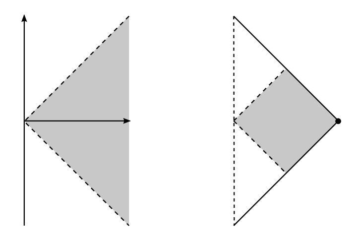
Figure 1: Left: The region $\tilde{\mathcal{D}}$, the complement of the light cone through the origin, in the physical Minkowski spacetime. Intuitively, this region contains spatial infinity. Right: the corresponding region $\mathcal{D}$ in the Penrose diagram of the Minkowski spacetime.

The inverse transformation is given by

$$\tilde{x}^{\mu}=-x^{\mu}/X^{2},\qquad X^{2}=\eta_{\mu\nu}x^{\mu}x^{\nu}.$$

Observe, in particular that $X^{2}=1/\tilde{X}^{2}$. Using these coordinates one identifies a conformal representation of the Minkowski spacetime with unphysical metric given by

$$\bar{\bm{\eta}}=\Xi^{2}\tilde{{\bm{\eta}}},\qquad\Xi\equiv X^{2},$$

where

$$\bar{\bm{\eta}}=\eta_{\mu\nu}\mathbf{d}x^{\mu}\otimes\mathbf{d}x^{\nu}.$$

Introducing an unphysical radial coordinate via the relation $\rho^{2}\equiv\delta_{\alpha\beta}x^{\alpha}x^{\beta}$, one finds that the metric $\bar{\bm{\eta}}$ can be written as

$$\bar{\bm{\eta}}=\mathbf{d}t\otimes\mathbf{d}t-\mathbf{d}\rho\otimes\mathbf{d}\rho-\rho^{2}\mathbf{\bm{\sigma}},\qquad\Xi=t^{2}-\rho^{2},$$

with $t\in(-\infty,\infty)$ and $\rho\in(0,\infty)$. In this conformal representation, spatial infinity $i^{0}$ corresponds to the origin of the domain

$$\mathcal{D}\equiv\{p\in\mathbb{R}^{4}\;|\;\eta_{\mu\nu}x^{\mu}(p)x^{\nu}(p)<0\}.$$

This region contains the asymptotic region of the Minkowski spacetime around spatial infinity. Observe that $(\tilde{t},\tilde{\rho})$ are related to $(t,\rho)$ via

$$\tilde{t}=-\dfrac{t}{t^{2}-\rho^{2}},\qquad\tilde{\rho}=-\dfrac{\rho}{t^{2}-\rho^{2}}.$$

Finally, introducing a time coordinate $\tau$ through the relation $t=\rho\tau$ one finds that the metric $\bar{\bm{\eta}}$ can be written as

$$\bar{\bm{\eta}}=\rho^{2}\mathbf{d}\tau\otimes\mathbf{d}\tau-(1-\tau^{2})\mathbf{d}\rho\otimes\mathbf{d}\rho+\rho\tau\mathbf{d}\rho\otimes\mathbf{d}\tau+\rho\tau\mathbf{d}\tau\otimes\mathbf{d}\rho-\rho^{2}{\bm{\sigma}}.$$

2.2 The cylinder at spatial infinity

The conformal representation containing the cylinder at spatial infinity is obtained by considering the rescaled metric

$${\bm{\eta}}\equiv\dfrac{1}{\rho^{2}}\bar{\bm{\eta}}.$$ (1)

Introducing the coordinate $\varrho\equiv-\ln\rho$ the metric ${\bm{\eta}}$ can be reexpressed as

$${\bm{\eta}}=\mathbf{d}\tau\otimes\mathbf{d}\tau-(1-\tau^{2})\mathbf{d}\varrho\otimes\mathbf{d}\varrho-\tau\mathbf{d}\tau\otimes\mathbf{d}\varrho-\tau\mathbf{d}\varrho\otimes\mathbf{d}\tau-\bm{\sigma}.$$

Observe that spatial infinity $i^{0}$, which is at infinity respect to the metric ${\bm{\eta}}$, corresponds to a set which has the topology of $\mathbb{R}\times\mathbb{S}^{2}$ —see [5, 1]. Following the previous discussion, one considers the conformal extension $(\mathcal{M},{\bm{\eta}})$ where

$${\bm{\eta}}=\Theta^{2}\tilde{{\bm{\eta}}},\qquad\Theta\equiv\rho(1-\tau^{2}),$$

and

$$\mathcal{M}\equiv\big{\{}p\in\mathbb{R}^{4}\;\rvert\;-1\leq\tau\leq 1,\;\;\rho(p)\geq 0\big{\}}.$$

In this representation future and past null infinity are described by the sets

$$\mathscr{I}^{+}\equiv\big{\{}p\in\mathcal{M}\;\rvert\;\tau(p)=1\big{\}},\qquad\mathscr{I}^{-}\equiv\big{\{}p\in\mathcal{M}\;\rvert\;\tau(p)=-1\big{\}},$$

while the physical Minkowski spacetime can be identified with the set

$$\tilde{\mathcal{M}}\equiv\big{\{}p\in\mathcal{M}\;\rvert\;-1<\tau(p)<1,\;\;\rho(p)>0\big{\}}.$$

In addition, the following sets play a role in our discussion:

$$\mathcal{I}\equiv\big{\{}p\in\mathcal{M}\;\rvert\;\;|\tau(p)|<1,\;\rho(p)=0\big{\}},$$

corresponding to the cylinder at spatial infinity, and

$$\mathcal{I}^{+}\equiv\big{\{}p\in\mathcal{M}\;\rvert\;\tau(p)=1,\;\rho(p)=0\big{\}},\qquad\mathcal{I}^{-}\equiv\big{\{}p\in\mathcal{M}\;\rvert\;\tau(p)=-1,\;\rho(p)=0\big{\}},$$

which describe the critical sets where null infinity touches spatial infinity. Additionally, let

$$\tilde{\mathcal{S}}_{\star}=\{p\in\mathbb{R}^{4}\;\rvert\;\tilde{t}(p)=0\},\qquad{\mathcal{S}}_{\star}=\{p\in\mathcal{M}\;\rvert\;\tau(p)=0\},$$

describing the time symmetric hypersurface of the Minkowski spacetime. The region where ${\mathcal{S}}_{\star}$ intersect $\mathcal{I}$ is denoted with $\mathcal{I}^{0}$.

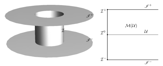
Figure 2: Left: schematic representation of the cylinder at spatial infinity of the Minkowski spacetime in the so-called F-gauge where null infinity corresponds to the locus of points with $\tau=\pm 1$. The cylinder $\mathcal{I}$ is a total characteristic of Maxwell-scalar field equations. Right: longitudinal section in which the angular dependence has been suppressed. Here $\mathcal{U}$ denotes an open set in a neighbourhood of $i$ and $\mathcal{M}(\mathcal{U})$ its development; $\mathcal{I}^{\pm}$ are the critical sets where the cylinder meets spatial infinity and $\mathcal{I}^{0}$ is the intersection of the cylinder with the initial hypersurface. These figures are coordinate rather than conformal diagrams —in particular, conformal geodesics correspond to vertical lines. Figure taken from Figure 20.3 in page 543 of [23]. ©Cambridge University Press. Reprinted with permission.

3 The Maxwell-scalar field system

In this section we provide a brief account of the Maxwell-scalar field system with particular attention to its conformal properties and formulation in terms of spinors.

3.1 Equations in the physical spacetime

In the following let $\tilde{F}_{ab}$ denote an antisymmetric tensor (the Faraday tensor) over a spacetime $(\tilde{\mathcal{M}},\tilde{{\bm{g}}})$ and let $\tilde{\nabla}$ be the Levi-Civita connection of the metric $\tilde{\bm{g}}$. The Maxwell equations with source are given by

$$\tilde{\nabla}^{a}\tilde{F}_{ab}=\tilde{J}_{b},$$ (2a)

$$\tilde{\nabla}_{[a}\tilde{F}_{bc]}=0.$$ (2b)

The homogeneous equation (2b) is automatically satisfied if one sets

$$\tilde{F}_{ab}=\tilde{\nabla}_{a}\tilde{A}_{b}-\tilde{\nabla}_{b}\tilde{A}_{a},$$

where $\tilde{A}_{a}$ denotes the 4-vector gauge potential. Coupled to the above, we consider the conformally invariant wave equation

$$\tilde{\mathfrak{D}}_{a}\tilde{\mathfrak{D}}^{a}\tilde{\phi}-\frac{1}{6}\tilde{R}\tilde{\phi}=0,$$ (3)

where $\tilde{\phi}$ denotes a complex scalar field. The coupling between the Maxwell field and the scalar field is encoded in the covariant derivative

$$\tilde{\mathfrak{D}}_{a}=\tilde{\nabla}_{a}-\mbox{i}\mathfrak{q}\tilde{A}_{a},$$

where $\mathfrak{q}$ is a coupling constant (the charge). The current $\tilde{J}_{a}$ in the inhomogeneous equation (2a) is given by

$$\tilde{J}_{a}=\mbox{i}\mathfrak{q}\bigg{(}\overline{\tilde{\phi}}\tilde{\mathfrak{D}}_{a}\tilde{\phi}-\tilde{\phi}\overline{(\tilde{\mathfrak{D}}_{a}\tilde{\phi})}\bigg{)}$$

3.1.1 Gauge invariance

The Maxwell-scalar field system (2a)-(2b) and (3) is invariant under the gauge transformation

$$\tilde{\phi}\rightarrow\tilde{\phi}^{\prime}=e^{\mathrm{i}\chi}\tilde{\phi},\qquad\tilde{A}_{a}\rightarrow\tilde{A}^{\prime}_{a}=\tilde{A}_{a}+\nabla_{a}\chi,$$ (4)

in the sense that $\tilde{F}_{ab}$ and $\tilde{J}_{a}$ are not affected by the transformation. Moroever, the Lorenz gauge condition

$$\tilde{\nabla}^{a}\tilde{A}_{a}=0,$$ (5)

is preserved by the transformation (4) for any $\chi$ such that

$$\square\chi=0.$$

Even with the Lorenz gauge condition imposed, there is some residual gauge freedom left. This residual gauge freedom can be fixed at the level of the initial conditions —in particular, there is a natural choice which allows to control the initial value of the components of $A_{a}$ and its derivatives by the energy of the system —see Section 5.

3.1.2 Conformal transformation properties

Consider a conformal rescaling of the form

$$g_{ab}=\Xi^{2}\tilde{g}_{ab}.$$

Associated to the latter we define the unphysical Faraday tensor, unphysical vector potential and the unphysical scalar field via

$$F_{ab}\equiv\tilde{F}_{ab},\qquad A_{a}\equiv\tilde{A}_{a},\qquad\phi\equiv\Xi^{-1}\tilde{\phi},$$

so that a computation using the standard conformal transformation formulae (see e.g. [23]) shows that

$$\nabla^{a}F_{ab}=J_{b},$$ (6a)

$$\nabla_{[a}F_{bc]}=0,$$ (6b)

$$F_{ab}=\nabla_{a}A_{b}-\nabla_{b}A_{a},$$ (6c)

$$\mathfrak{D}_{a}\mathfrak{D}^{a}\phi-\frac{1}{6}R\phi=0,$$ (6d)

where

$$\mathfrak{D}_{a}\equiv\nabla_{a}-\mbox{i}\mathfrak{q}A_{a}$$

and

$$J_{a}=\mbox{i}\mathfrak{q}\bigg{(}\overline{\phi}\mathfrak{D}_{a}\phi-\phi\overline{(\mathfrak{D}_{a}\phi)}\bigg{)}.$$ (7)

In particular, it follows that

$$\tilde{J}_{a}=\Xi^{2}J_{a}.$$

Moreover, one can verify that

$$\nabla^{a}J_{a}=0.$$

Introducing the Hodge dual $F^{*}_{ab}$ of the Faraday tensor in the usual way via

$$F^{*}_{ab}\equiv\frac{1}{2}\epsilon_{ab}{}^{cd}F_{cd},$$

the Maxwell equation (6b) can be rewritten as

$$\nabla^{a}F^{*}_{ab}=0.$$ (8)

3.2 Spinorial expressions

In this subsection we provide the spinorial version of the equations in the unphysical spacetime.

Let $F_{AA^{\prime}BB^{\prime}}$ denote the spinorial counterpart of the Faraday tensor $F_{ab}$. It satisfies the well-know decomposition

$$F_{AA^{\prime}BB^{\prime}}=\phi_{AB}\epsilon_{A^{\prime}B^{\prime}}+\bar{\phi}_{A^{\prime}B^{\prime}}\epsilon_{AB},$$

where $\phi_{AB}=\phi_{(AB)}$ is the so-called Maxwell spinor —see e.g. [14, 23]. A calculation with this expression shows that equations (6a) and (8) are equivalent to

$$\nabla^{B}{}_{A^{\prime}}\phi_{AB}=J_{AA^{\prime}},$$ (9)

where

$$J_{AA^{\prime}}\equiv\mbox{i}\mathfrak{q}\bigg{(}\bar{\phi}\nabla_{AA^{\prime}}\phi-\phi\nabla_{AA^{\prime}}\bar{\phi}\bigg{)}+2\mathfrak{q}^{2}|\phi|^{2}A_{AA^{\prime}},$$

is the spinorial counterpart of the current $J_{a}$ and $A_{AA^{\prime}}$ is the spinorial counterpart of the vector potential $A_{a}$. Observe that both $A_{AA^{\prime}}$ and $J_{AA^{\prime}}$ are Hermitian spinors. In view of its symmetries, equation (6c) can be rewritten as

$$\phi_{AB}=\nabla_{A^{\prime}(A}A_{B)}{}^{A^{\prime}}.$$ (10)

3.2.1 The wave equation for the vector potential and the generalised Lorenz gauge

It is well known that in the Lorenz gauge, the vector potential satisfies a wave equation. In light of the Lorenz gauge condition in spinorial form

$$\nabla^{AA^{\prime}}A_{AA^{\prime}}=0,$$ (11)

it is possible to remove the symmetrisation in equation (10) so as to obtain

$$\nabla_{AA^{\prime}}A_{B}{}^{A^{\prime}}=\phi_{AB}.$$ (12)

Applying $\nabla^{A}{}_{B^{\prime}}$, using the spinorial Maxwell equation (9) and making use of the commutator of the covariant derivative $\nabla_{AA^{\prime}}$ one obtains

$$\square A_{BB^{\prime}}+2\Phi_{AA^{\prime}BB^{\prime}}A^{AA^{\prime}}=J_{BB^{\prime}}.$$

Now, since

$$J_{BB^{\prime}}=2\mathfrak{q}^{2}|\phi|^{2}A_{BB^{\prime}}+\mbox{i}\bar{\phi}\nabla_{BB^{\prime}}\phi-\mbox{i}\mathfrak{q}\phi\nabla_{BB^{\prime}}\bar{\phi}$$

the wave equation for the vector potential reads as

$$\square A_{BB^{\prime}}+2\Phi_{AA^{\prime}BB^{\prime}}A^{AA^{\prime}}=2\mathfrak{q}^{2}|\phi|^{2}A_{BB^{\prime}}+\mbox{i}\mathfrak{q}\bar{\phi}\nabla_{BB^{\prime}}\phi-\mbox{i}\mathfrak{q}\phi\nabla_{BB^{\prime}}\bar{\phi}.$$

3.2.2 The wave equation for the Maxwell spinor

The unphysical charged wave equation is given by

$$g^{ab}\mathfrak{D}_{a}\mathfrak{D}_{b}\phi-\frac{R\phi}{6}=0.$$

This equation can be recast in spinor formalism by replacing

$$\mathfrak{D}_{a}=\nabla_{a}-\mbox{i}\mathfrak{q}A_{a}$$

and then by separating the soldering forms so that we have

$$\square\phi=\mathfrak{q}^{2}\phi A_{AA^{\prime}}A^{AA^{\prime}}+2\mathrm{i}\mathfrak{q}A^{AA^{\prime}}\nabla_{AA^{\prime}}\phi+\mathrm{i}\mathfrak{q}\phi\nabla_{AA^{\prime}}A^{AA^{\prime}}.$$

Hence, by using the Lorenz gauge condition (11) we have

$$\square\phi=\mathfrak{q}^{2}\phi A_{AA^{\prime}}A^{AA^{\prime}}+2\mathrm{i}\mathfrak{q}A^{AA^{\prime}}\nabla_{AA^{\prime}}\phi.$$

3.2.3 Summary

In summary, the study of the Maxwell-scalar field system can be reduced, making use of the generalised Lorenz gauge condition (11), to the system of wave equations

$$\square\phi=\mathfrak{q}^{2}\phi A_{AA^{\prime}}A^{AA^{\prime}}+2\mathrm{i}\mathfrak{q}A^{AA^{\prime}}\nabla_{AA^{\prime}}\phi,$$ (13a)

$$\square A_{AA^{\prime}}+2\Phi_{ABA^{\prime}B^{\prime}}A^{BB^{\prime}}=2\mathfrak{q}|\phi|^{2}A_{AA^{\prime}}+\mbox{i}\mathfrak{q}\bar{\phi}\nabla_{AA^{\prime}}\phi-\mbox{i}\mathfrak{q}\phi\nabla_{AA^{\prime}}\bar{\phi}.$$ (13b)

These equations are supplemented by initial conditions for the values of $\phi$ and $A_{AA^{\prime}}$ and of their normal derivatives. This will be discussed in more detail in Section 5.

3.3 Decomposition of the equations in the space-spinor formalism

Before providing a detailed decomposition of the equations (13a)-(13b), it is convenient to provide a rougher decomposition which brings to the foreground the structural properties of the evolution system and its relation to the Maxwell constraint equations. This decomposition is done using the space-spinor formalism as described in e.g. [23] —see also [2, 13].

3.3.1 Basic relations

Let $\tau^{AA^{\prime}}$ denote the spinorial counterpart of a timelike vector field $\tau^{a}$ tangent to a congruence of curves. The Hermitian spinor $\tau^{AA^{\prime}}$ is chosen to have the normalisation

$$\tau_{AA^{\prime}}\tau^{AA^{\prime}}=2.$$

Consistent with the latter, we consider a spin dyad $\{o^{A},\,\iota^{A}\}$ chosen so that

$$\tau^{AA^{\prime}}=o^{A}\bar{o}^{A^{\prime}}+\iota^{A}\bar{\iota}^{A^{\prime}}.$$

It follows then that

$$\tau_{AA^{\prime}}\tau^{BA^{\prime}}=\delta_{A}{}^{B}.$$

The above relations induce a Hermitian conjugation operation via the relation

$$\mu^{\dagger}_{A}\equiv\tau_{A}{}^{A^{\prime}}\bar{\mu}_{A^{\prime}},$$

with the obvious extension to higher valence spinors. In particular, one has that $\iota_{A}=o^{\dagger}_{A}$. The space-spinor allows to work with spinors with unprimed indices. In this spirit one has the following decompositions for the spinorial counterpart of the current vector and the vector potential:

$$J_{AA^{\prime}}=\tfrac{1}{2}j\tau_{AA^{\prime}}-j_{AB}\tau^{B}{}_{A^{\prime}},$$ (14a)

$$A_{AA^{\prime}}=\tfrac{1}{2}\alpha\tau_{AA^{\prime}}-\alpha_{AB}\tau^{B}{}_{A^{\prime}},$$ (14b)

with $j_{AB}$ and $\alpha_{AB}$ symmetric spinors.

Decomposition of the covariant derivative. The spinor $\tau^{AA^{\prime}}$ also induces a decomposition of the spinorial covariant derivatives $\nabla_{AA^{\prime}}$. For this, one defines the differential operators

$$\mathcal{D}\equiv\tau^{AA^{\prime}}\nabla_{AA^{\prime}},\qquad\mathcal{D}_{AB}\equiv\tau_{(A}{}^{A^{\prime}}\nabla_{B)A^{\prime}}.$$

The covariant derivatives $\mathcal{D}$ and $\mathcal{D}_{AB}$ correspond, respectively, to the Fermi and Sen connections associated to the congruence defined by $\tau^{a}$.

The Maxwell equations in space-spinor form. Some manipulations show that the spinorial Maxwell equation (9) can be decomposed as

$$\mathcal{D}^{AB}\phi_{AB}=\tfrac{1}{2}j,$$

$$\mathcal{D}\phi_{AB}-2\mathcal{D}^{Q}{}_{(A}\phi_{B)Q}=-j_{AB}.$$

The former equation is to be interpreted as a constraint while the latter as evolution equations —in fact, it can be shown to be (up to some numerical factors) a symmetric hyperbolic system for the independent components of $\phi_{AB}$, see [23]. Similarly, from equation (12) one obtains the system

$$\mathcal{D}\alpha+2\mathcal{D}^{AC}\alpha_{AC}+\sqrt{2}\alpha\chi^{AC}{}_{AC}-2\sqrt{2}\alpha^{AC}\chi_{A}{}^{B}{}_{CB}-\chi^{AC}\alpha_{AC}=2\mathcal{A}(x),$$

$$\mathcal{D}\alpha_{CD}-\mathcal{D}_{CD}\alpha-\sqrt{2}\alpha\chi_{(C}{}^{A}{}_{D)A}-2\mathcal{D}_{(C}{}^{A}\alpha_{D)A}-\chi_{(C}{}^{A}\alpha_{D)A}$$

$$\hskip 142.26378pt+2\sqrt{2}\alpha^{AB}\chi_{(C|A|D)B}+\tfrac{1}{2}\alpha\chi_{CD}=2\hat{\phi}_{CD},$$

where $\chi_{AB}$ and $\chi_{ABCD}$ are, respectively, the acceleration and Weingarten spinors defined by the relation

$$\nabla_{AA^{\prime}}\tau_{CC^{\prime}}=-\tfrac{1}{2}\chi_{CD}\tau_{AA^{\prime}}\tau^{D}{}_{C^{\prime}}+\sqrt{2}\chi_{ABCD}\tau^{B}{}_{A^{\prime}}\tau^{D}{}_{C^{\prime}}.$$

and where

$$\hat{\phi}_{AB}\equiv\tau_{A}{}^{C^{\prime}}\tau_{B}{}^{D^{\prime}}\bar{\phi}_{C^{\prime}D^{\prime}}$$

is the Hermitian conjugate of $\phi_{AB}$.

The scalar field. It is also illustrative to express equation (13a) in terms of the Fermi and the Sen connections $\mathcal{D}$ and $\mathcal{D}_{AB}$. Making use of the decomposition

$$\nabla_{AA^{\prime}}=\tfrac{1}{2}\tau_{AA^{\prime}}\mathcal{D}-\tau^{Q}{}_{A^{\prime}}\mathcal{D}_{AQ},$$

a calculation gives that

$$\mathcal{D}^{2}\phi+2\mathcal{D}_{AB}\mathcal{D}^{AB}=-\sqrt{2}\chi^{AB}{}_{AB}\mathcal{D}\phi+\chi^{AB}\mathcal{D}_{AB}\phi+2\sqrt{2}\chi_{A}{}^{Q}{}_{BC}\mathcal{D}^{AB}\phi.$$

Remark 1.

The equations presented in this section are completely general and make no assumption on the background spacetime. When evaluated on a the conformal representation of the Minkowski spacetime discussed in Section 2.2 they acquire a much simpler form.

3.3.2 Detailed decomposition in conformal Minkowski

In this section we particularise the decomposition of the various fields to the case of the conformal representation of Minkowski spacetime discussed in Section 2.2.

Frame choice. Following [6] we consider a so-called Newman-Penrose (NP) frame satisfying

$${\bm{g}}({\bm{e}}_{{\bm{A}}{\bm{A}}^{\prime}},{\bm{e}}_{{\bm{B}}{\bm{B}}^{\prime}})=\epsilon_{{\bm{A}}{\bm{B}}}\epsilon_{{\bm{A}}^{\prime}{\bm{B}}^{\prime}},$$

of the form

$${\bm{e}}_{{\bm{0}}{\bm{0}}^{\prime}}=\frac{1}{\sqrt{2}}\bigg{(}(1-\tau){\bm{\partial}}_{\tau}+\rho{\bm{\partial}}_{\rho}\bigg{)},$$

$${\bm{e}}_{{\bm{1}}{\bm{1}}^{\prime}}=\frac{1}{\sqrt{2}}\bigg{(}(1+\tau){\bm{\partial}}_{\tau}-\rho{\bm{\partial}}_{\rho}\bigg{)},$$

$${\bm{e}}_{{\bm{0}}{\bm{1}}^{\prime}}=-\frac{1}{\sqrt{2}}{\bm{X}}_{+},$$

$${\bm{e}}_{{\bm{1}}{\bm{0}}^{\prime}}=-\frac{1}{\sqrt{2}}{\bm{X}}_{-},$$

where ${\bm{X}}_{+}$ and ${\bm{X}}_{-}$ are vectors spanning the tangent space of $\mathbb{S}^{2}$ with dual covectors ${\bm{\alpha}}_{+}$ and ${\bm{\alpha}}_{-}$ such that metric of the 2-sphere is given by

$${\bm{\sigma}}=2({\bm{\alpha}}^{+}\otimes{\bm{\alpha}}^{-}+{\bm{\alpha}}^{-}\otimes{\bm{\alpha}}^{+}).$$

The vector $\tau^{a}$ giving rise to the space-spinor decomposition of the Maxwell-scalar field introduced in Section 3.3 is chosen as

$$\tau^{a}=e_{{\bm{0}}{\bm{0}}^{\prime}}{}^{a}+e_{{\bm{1}}{\bm{1}}^{\prime}}{}^{a}=\sqrt{2}({\bm{\partial}}_{\tau})^{a}.$$

A peculiarity of the conformal representation introduced in equation (1) is that the Ricci scalar vanishes —that is,

$$R[{\bm{g}}]=0.$$

The reduced wave equations. As the expression of the wave operator in the F-gauge acting on a spin-weighted scalar will be used repeatedly , it is convenient to define the F-reduced wave operator $\blacksquare$ acting on a scalar $\zeta$ as

$$\blacksquare\zeta\equiv(1-\tau^{2})\ddot{\zeta}+2\tau\rho\dot{\zeta}^{\prime}-\rho^{2}\zeta^{\prime\prime}-2\tau\dot{\zeta}-\frac{1}{2}\eth\bar{\eth}\zeta-\frac{1}{2}\bar{\eth}\eth\zeta,$$ (15)

where for simplicity of the presentation we have used the notation

$$\dot{\phantom{X}}\equiv\partial_{\tau},\qquad\phantom{X}^{\prime}\equiv\partial_{\rho},$$

and $\eth$ and $\bar{\eth}$ denote the NP eth and eth bar operators —see e.g. [11, 14]. In particular, the operator $\tfrac{1}{2}(\eth\bar{\eth}-\bar{\eth}\eth)$ corresponds to the Laplacian on $\mathbb{S}^{2}$.

After some lengthy computations, best carried out using the suite xAct for tensorial and spinorial manipulations in the Wolfram programming language [10], the wave equations (13a)-(13b) can be seen to be equivalent to the scalar system:

$$\blacksquare\phi=\mathfrak{q}^{2}\phi\bigg{(}\frac{1}{2}\alpha^{2}-2\alpha_{1}^{2}+2\alpha_{0}\alpha_{2}\bigg{)}+\mathrm{i}\sqrt{2}\mathfrak{q}\big{(}2\alpha_{1}\rho\phi^{\prime}+\alpha\dot{\phi}-2\tau\alpha_{1}\dot{\phi}+\alpha_{0}\eth\phi-\alpha_{2}\bar{\eth}\phi\big{)},$$

$$\blacksquare\alpha-4\dot{\alpha}_{1}=2\mathfrak{q}^{2}\alpha|\phi|^{2}+\mbox{i}\sqrt{2}\mathfrak{q}\big{(}\dot{\phi}\bar{\phi}-\dot{\bar{\phi}}\phi\big{)},$$

$$\blacksquare\alpha_{0}+\alpha_{0}=2\mathfrak{q}^{2}\alpha_{0}|\phi|^{2}+\frac{\mathrm{i}\mathfrak{q}}{\sqrt{2}}(\phi\bar{\eth}\bar{\phi}-\bar{\phi}\bar{\eth}\phi),$$

$$\blacksquare\alpha_{1}-\dot{\alpha}=2\mathfrak{q}^{2}\alpha_{1}|\phi|^{2}+\frac{\mathrm{i}\mathfrak{q}\rho}{\sqrt{2}}(\phi\bar{\phi}^{\prime}-\bar{\phi}\phi^{\prime})+\frac{\mathrm{i}\mathfrak{q}\tau}{\sqrt{2}}(\bar{\phi}\dot{\phi}-\phi\dot{\bar{\phi}}),$$

$$\blacksquare\alpha_{2}+\alpha_{2}=2\mathfrak{q}^{2}\alpha_{2}|\phi|^{2}+\frac{\mathrm{i}\mathfrak{q}}{\sqrt{2}}(\bar{\phi}\eth\phi-\phi\eth\bar{\phi}).$$

The scalars $\alpha$, $\alpha_{0}$, $\alpha_{1}$ and $\alpha_{2}$ have spin weight $0,\;1,\;0,\;-1$, respectively. In particular, $\alpha$ denotes the time component of the Hermitian spinor $A_{AA^{\prime}}$ while $\alpha_{0},\;\alpha_{1},\;\alpha_{2}$ are the independent components of its spatial part —cfr. the decomposition in equation (14b).

It is observed that the righthand sides of the above wave equations can be decoupled if one defines

$$\alpha_{\pm}\equiv\alpha\pm\alpha_{1},\qquad j_{\pm}\equiv j\pm j_{1},$$

all of them of spin-weight $0$. In terms of these new variables the system of wave equations can be rewritten as

$$\blacksquare\phi=s,$$

$$\blacksquare\alpha_{+}-2\dot{\alpha}_{+}=j_{+},$$

$$\blacksquare\alpha_{-}+2\dot{\alpha}_{-}=j_{-},$$

$$\blacksquare\alpha_{0}+\alpha_{0}=j_{0},$$

$$\blacksquare\alpha_{2}+\alpha_{2}=j_{2},$$

with the obvious definitions. For future use, it is observed that the source terms

$$s=s(\bar{x},\phi,\alpha_{0},\alpha_{2},\alpha_{\pm}),$$

$$j_{0}=j_{0}(\bar{x},\phi,\alpha_{0},\alpha_{2},\alpha_{\pm}),\qquad j_{2}=j_{2}(\bar{x},\phi,\alpha_{0},\alpha_{2},\alpha_{\pm}),\qquad j_{\pm}=j_{\pm}(\bar{x},\phi,\alpha_{0},\alpha_{2},\alpha_{\pm}),$$

are at most cubic polynomial expression in the unknowns $\phi,\,\alpha_{0},\,\alpha_{2},\,\alpha_{\pm}$.

4 General structural properties and expansions near spatial infinity

In this section we discuss general structural properties of the evolution system, equations (24a)-(24e), associated to the Maxwell-scalar field system. In particular, we study a type of asymptotic expansions near spatial infinity which was first introduced, for the conformal Einstein field equations, by H. Friedrich in [5]. In the following, we refer to these expansions as F-expansions. This construction exploits the fact that the cylinder at spatial infinity, $\mathcal{I}$, introduced in Section 2.2 is a total characteristic of the evolution equations associated to the Maxwell-scalar system. Accordingly, the evolution equations reduce to an interior system (transport equations) upon evaluation on the cylinder $\mathcal{I}$. This can clearly seen from the form of the reduced wave operator $\blacksquare$ as given by equation (15) —all the $\partial_{\rho}$ derivatives disappear from the equation if one sets $\rho=0$. These transport equations allow to relate properties of the initial data, as defined on a fiduciary initial hypersurface $\mathcal{S}_{\star}$, with radiative properties of the solution which are defined at null infinity $\mathscr{I}^{\pm}$.

For convenience of the subsequent discussion we define

$${\bm{\alpha}}\equiv\left(\begin{array}[]{c}\alpha_{+}\\ \alpha_{-}\\ \alpha_{0}\\ \alpha_{2}\end{array}\right),\qquad{\bm{j}}\equiv\left(\begin{array}[]{c}j_{+}\\ j_{-}\\ j_{0}\\ j_{2}\end{array}\right),\qquad\mathbf{A}\equiv\left(\begin{array}[]{cccc}-2&0&0&0\\ 0&2&0&0\\ 0&0&0&0\\ 0&0&0&0\end{array}\right),\qquad\mathbf{B}\equiv\left(\begin{array}[]{cccc}0&0&0&0\\ 0&0&0&0\\ 0&0&1&0\\ 0&0&0&1\end{array}\right).$$

In terms of the above vectors an matrices the system (24a)-(24e) can be rewritten as

$$\blacksquare\phi=s,$$ (16a)

$$\blacksquare{\bm{\alpha}}+\mathbf{A}\dot{\bm{\alpha}}+\mathbf{B}{\bm{\alpha}}={\bm{j}}.$$ (16b)

The source terms can, in turn, be written as

$$s=\phi{\bm{\alpha}}^{\dagger}\mathbf{Q}{\bm{\alpha}}+{\bm{\alpha}}^{\dagger}\mathbf{K}(x){\bm{\partial}}\phi,$$

$${\bm{j}}=2\mathfrak{q}|\phi|^{2}{\bm{\alpha}}+\phi\mathbf{L}{\bm{\partial}}\bar{\phi}+\bar{\phi}\mathbf{L}{\bm{\partial}}\phi,$$

where ^† denotes the Hermitian transpose of a vector (i.e. transposition plus complex conjugation), $\mathbf{Q}$ is a constant matrix, while $\mathbf{K}(x)$ and $\mathbf{L}(x)$ are coordinate-dependent matrices. Observe that if $\mathfrak{q}=0$ then $\mathbf{K}(x)=\mathbf{L}(x)=0$.

4.1 Transport equations on the cylinder at spatial infinity

The key observation in our analysis is that the F-reduced wave operator $\blacksquare$, as defined by (15), reduces to an operator intrinsic to $\mathcal{I}$. Defining the F-reduced wave operator on $\mathcal{I}$, $\blacktriangle\equiv\blacksquare|_{\mathcal{I}}$, acting on a scalar $\zeta$ as

$$\blacktriangle\zeta\equiv(1-\tau^{2})\ddot{\zeta}-2\tau\dot{\zeta}-\frac{1}{2}(\eth\bar{\eth}+\bar{\eth}\eth)\zeta.$$

one readily observes that this operator is intrinsic to $\mathcal{I}$. An alternative way of expressing this observation is that the cylinder at spatial infinity is a total characteristic of the evolution system (16a)-(16b).

Remark 2.

The intrinsic operator $\blacktriangle$ is clearly hyperbolic for $|\tau|<1$. However, at $\tau=\pm 1$ it degenerates. To investigate the effect of this degeneracy at the critical sets $\mathcal{I}^{\pm}$ it is convenient to study the transport equations implied by evolution equations.

4.1.1 The leading order transport equations

Evaluating equations (16a)-(16b) on $\mathcal{I}$ (i.e. at $\rho=0$) one obtains the interior system of wave equations:

$$\blacktriangle\phi^{(0)}=\phi^{(0)}{\bm{\alpha}}^{(0)\dagger}\mathbf{Q}{\bm{\alpha}}^{(0)}+{\bm{\alpha}}^{(0)\dagger}\mathbf{K}{\bm{\partial}}\phi^{(0)},$$ (17a)

$$\blacktriangle{\bm{\alpha}}^{(0)}+\mathbf{A}\dot{\bm{\alpha}}^{(0)}+\mathbf{B}{\bm{\alpha}}^{(0)}=2\mathfrak{q}|\phi^{(0)}|^{2}{\bm{\alpha}}^{(0)}+\phi^{(0)}\mathbf{L}{\bm{\partial}}\bar{\phi}^{(0)}+\bar{\phi}^{(0)}\mathbf{L}{\bm{\partial}}\phi^{(0)},$$ (17b)

with

$$\phi^{(0)}\equiv\phi|_{\mathcal{I}},\qquad{\bm{\alpha}}^{(0)}\equiv{\bm{\alpha}}|_{\mathcal{I}}.$$

Initial data for the system (17a)-(17b) is provided by the restriction of the initial data for the fields $\phi$, $\dot{\phi}$, ${\bm{\alpha}}$ and $\dot{\bm{\alpha}}$ on $\mathcal{S}_{\star}$ to $\mathcal{I}$.

Remark 3.

The interior system (17a)-(17b) is, in principle, coupled and non-linear. However, certain classes of initial data allow for a decoupling of the system. This feature is discussed in Section 6.

4.1.2 Higher order transport equations

Making use of the structural properties of the evolution system (16a)-(16b) it is possible to consider higher order generalisations of the transport equations introduced the previous subsection. To this end, one consider the commutator

$$\partial_{\rho}^{p}\blacksquare\zeta-\blacksquare\partial_{\rho}^{p}\zeta=2\tau p\partial_{\rho}^{p}\dot{\zeta}-2p\rho\partial_{\rho}^{p}\zeta^{\prime}-p(p-1)\partial_{\rho}^{p}\zeta,$$

with $\partial^{p}_{\rho}$ denoting $p$ applications of the derivative $\partial_{\rho}$. Now, applying the operator $\partial_{\rho}$ to equations (16a)-(16b) a total number of $p$ times and restricting to $\mathcal{I}$ one finds that

$$\blacktriangle\phi^{(p)}+2\tau p\dot{\phi}^{(p)}-p(p-1)\phi^{(p)}=s^{(p)},$$

$$\blacktriangle{\bm{\alpha}}^{(p)}+\mathbf{A}\dot{\bm{\alpha}}^{(p)}+2\tau p\dot{{\bm{\alpha}}}^{(p)}+\mathbf{B}{\bm{\alpha}}^{(p)}-p(p-1){\bm{\alpha}}^{(p)}=\mathbf{R}^{(p)},$$

where $s^{(p)}$ and $\mathbf{R}^{(p)}$ denote source terms which depend on the solutions of the lower order transport equations —i.e. $(\phi^{(p^{\prime})},\,{\bm{\alpha}}^{(p^{\prime})})$ for $p^{\prime}$ such that $0\leq p^{\prime}\leq p-1$. This observation allows to implement a recursive scheme to compute the solutions to the transport equations to any arbitrary order —module computational complexities.

5 Initial conditions

In this section we discuss the construction of initial data for the Maxwell-scalar field system in the Lorenz gauge. Accordingly, throughout it is assumed that

$$\nabla^{a}A_{a}=0.$$

5.1 General remarks

The wave equations (13a)-(13b) suggest that a natural prescription of initial data for the Maxwell-scalar field system is

$$\phi_{\star},\qquad\mathcal{D}\phi_{\star},\qquad A_{AA^{\prime}\star},\qquad\mathcal{D}A_{AA^{\prime}\star}.$$

Notice that the components of $A_{AA^{\prime}}$ and $\mathcal{D}A_{AA^{\prime}\star}$ cannot be prescribed freely. Moreover, there is some gauge freedom that can be used to set certain components to zero —see below.

Remark 4.

The above is not necessarily the most physical way of prescribing initial conditions. A more physical choice is to prescribe

$$\phi_{\star},\qquad\mathcal{D}\phi_{\star},\qquad\eta_{AB\star},\qquad\mu_{AB\star},$$

where $\eta_{AB}$ and $\mu_{AB}$ denote, respectively, the spinorial counterparts of the electric and magnetic parts of the Faraday tensor respect to the normal to the initial hypersurface $\mathcal{S}_{\star}$. In order to fix the asymptotic behaviour one requires finiteness of the energy

$$\mathcal{E}_{\star}\equiv\frac{1}{2}\int_{\mathbb{R}^{3}}\big{(}|\mathfrak{D}\phi_{\star}|^{2}+|{\bm{\eta}}_{\star}|^{2}+|{\bm{\mu}}_{\star}|^{2}\big{)}\mathrm{d}\mu.$$ (18)

In addition, the electric and magnetic parts are subject to the Gauss constraints implied by the equation

$$\mathcal{D}^{AB}\phi_{AB}=\tfrac{1}{2}j.$$

5.2 Data on time symmetric hypersurfaces

In the following we assume, for simplicity, that the initial hypersurface $\mathcal{S}_{\star}$ is the time symmetric hypersurface with $t=\mbox{constant}$ in the Minkowski spacetime. Accordingly the extrinsic curvature vanishes in this hypersurface —thus, we have that in the initial hypersurface $\mathcal{D}_{AB}=D_{AB}$ —that is, the Sen connection coincides with the Levi-Civita connection of the intrinsic metric to $\mathcal{S}_{\star}$. Notice, however, that it is not assumed that the acceleration vanishes on the initial hypersurface —this is for consistency with the conformal Gaussian gauge used to write the evolution equations.

Following the discussion in [12] we make use of the residual gauge freedom in the Lorenz gauge to set the initial value of the time components of $A_{a}$ and $\mathcal{D}A_{a}$ to zero initially. In terms of the space-spinor split of $A_{a}$ this is equivalent to requiring

$$\alpha_{\star}=0,\qquad\mathcal{D}\alpha_{\star}=0.$$

It follows then from the Lorenz gauge condition that

$$D^{AB}\alpha_{AB}=\tfrac{1}{2}\chi^{AB}\alpha_{AB}.$$ (19)

This equation has to be treated as a constraint on the spatial part $\alpha_{AB}$. Observe how this last equation involves the acceleration.

The definition of the Maxwell spinor in terms of $A_{AA^{\prime}}$ yields the condition

$$\phi_{AB}=-\tfrac{1}{2}\dot{\alpha}_{AB}-D_{(A}{}^{Q}\alpha_{B)Q},\qquad\mbox{on}\quad\mathcal{S}_{\star},$$

where for brevity we have written $\dot{\alpha}_{AB}\equiv\mathcal{D}\alpha_{AB}$. Substituting this relation into the Gauss constraint

$$D^{AB}\phi_{AB}=\tfrac{1}{2}j$$

one concludes that

$$D^{AB}\dot{\alpha}_{AB}=-j.$$ (20)

5.2.1 Solving the constraints for $\alpha_{AB}$ and $\dot{\alpha}_{AB}$

In order to solve the constraint equations (19) and (20) one can make use of the Ansatz

$$\alpha_{AB}=D_{AB}\sigma+D_{(A}{}^{Q}\sigma_{B)Q},$$ (21a)

$$\dot{\alpha}_{AB}=D_{AB}\pi+D_{(A}{}^{Q}\pi_{B)Q},$$ (21b)

with $\sigma$, $\pi$ scalars and $\sigma_{AB}$, $\pi_{AB}$ symmetric, real valence 2 spinors —the latter is essentially a spinorial version of the Helmholtz decomposition. The substitution of the Ansatz (21a)-(21b) in the constraints (19) and (20) leads to elliptic equations for the scalars $\sigma$, $\pi$. The spinors $\sigma_{AB}$ and $\pi_{AB}$ are free data.

5.2.2 Time symmetric initial conditions

Time symmetric initial data conditions for the Maxwell-scalar system, i.e. initial conditions giving rise to solutions which are time reflection symmetric with respect to the hypersurface $\mathcal{S}_{\star}$, are set by requiring

$$\dot{\phi}=0,\qquad\dot{\alpha}_{AB}=0,\qquad\mbox{on}\quad\mathcal{S}_{\star}.$$

It follows from the above that $j=0$. Thus, the only constraint equation left to solve is equation (19) which can then be solved using the Ansatz (21a). A further consequence of $\dot{\alpha}_{AB}=0$ is that

$$\phi_{AB}=-D_{(A}{}^{Q}\alpha_{B)Q},\qquad\hat{\phi}_{AB}=-D_{(A}{}^{Q}\alpha_{B)Q}.$$

Now, defining the electric and magnetic parts of $\phi_{\star}$ with respect to the Hermitian spinor $\tau^{AA^{\prime}}$ by

$$\eta_{AB}\equiv\tfrac{1}{2}\mathrm{i}(\phi_{AB}+\hat{\phi}_{AB}),\qquad{\mu}_{AB}\equiv\tfrac{1}{2}(\phi_{AB}-\hat{\phi}_{AB}),$$

one readily finds that

$$\mu_{AB}=0,\qquad\mbox{on}\quad\mathcal{S}_{\star}.$$

Remark 5.

This is the spinorial version of the well-known result stating that the magnetic part of time symmetric data for the Maxwell field has vanishing magnetic part.

5.2.3 Asymptotic conditions

The asymptotic behaviour of the initial data can be fixed in a natural way from the requirement of the finiteness of the energy on the (physical) initial hypersurface.

Scalar field. The finiteness of the energy as defined by equation (18) requires

$$\tilde{\mathfrak{D}}_{a}\tilde{\phi}_{\star}=o(\tilde{r}^{-1}),\qquad(\tilde{\eta}_{{\bm{A}}{\bm{B}}})_{\star}=o(\tilde{r}^{-1}),\qquad(\tilde{\mu}_{{\bm{A}}{\bm{B}}})_{\star}=o(\tilde{r}^{-1}).$$

These conditions are satisfied if

$$\tilde{\phi}_{\star}=o(\tilde{r}^{-1/2}),\qquad(\tilde{\alpha}_{{\bm{A}}{\bm{B}}})_{\star}=o(\tilde{r}^{-1/2}).$$

In particular, one can consider an initial scalar field with leading behaviour given by

$$\tilde{\phi}_{\star}=\mathring{\varphi}\tilde{r}^{-1}+\cdots,\qquad\mbox{with}\quad\mathring{\varphi}\quad\mbox{a constant}.$$

In order to obtain the conformal version of the above condition recall that $\Theta=\rho(1-\tau^{2})$ and, moreover, $\tilde{r}=1/\rho$ and $\varpi=\Theta_{\star}=\tilde{r}^{-1}=\rho$. Thus,

$$\phi_{\star}=\varpi^{-1}\tilde{\phi}_{\star}=\rho^{-1}\tilde{\phi}_{\star}=\mathring{\varphi}+\cdots.$$

For simplicity one can assume that $\phi_{\star}$ is analytic in a neighbourhood of spatial infinity.

Electric field. To analyse the asymptotic behaviour of the electric part of the Maxwell field from the conformal point of view, it is observed that

$$\tau^{a}=\varpi^{-1}\tilde{\tau}^{a},$$

where $\tilde{\tau}^{a}$ and $\tau^{a}$ are, respectively, the physical and unphysical normals to the initial hypersurface $\mathcal{S}_{\star}$. Accordingly, for a Coulomb-type field $\tilde{E}_{i}=O(1/\tilde{r}^{2})$ it follows that

$$E_{i}=\varpi^{-1}\tilde{E}_{i}=O(\rho).$$

In terms of the components with respect to the frame one has

$$E_{\bm{i}}=O(1),\qquad\eta_{{\bm{A}}{\bm{B}}}=O(1).$$

Gauge potential. For the gauge potential one has that $\tilde{A}_{a}=A_{a}$. Moreover, for a Coulomb-type field one has $\tilde{A}_{a}=O(1/\tilde{r})$ so that in terms of the spatial components with respect to the frame:

$$A_{\bm{i}}=O(1),\qquad\alpha_{{\bm{A}}{\bm{B}}}=O(1).$$

5.2.4 An Ansatz for the initial data

In order to give a more concrete Ansatz for the construction of the initial data for the Maxwell-scalar field system, in the following it will be assumed that the freely specifiable data $\phi_{\star}$ and $\sigma_{{\bm{A}}{\bm{B}}}$ are analytic in a neighbourhood of spatial infinity. It follows then from the ellipticity of the equation for the $\sigma$ that this scalar will also be analytic in a neighbourhood of $i^{0}$. Consistent with the above let

$$\phi_{\star}=\sum_{n=0}^{\infty}\sum_{l=0}^{n}\sum_{m=-1}^{l}\frac{1}{n!}\varphi_{n;l,m}(Y_{lm})\rho^{n},$$ (22a)

$$\sigma_{i}=\sum_{n=|1-i|}^{\infty}\sum_{l=|1-i|}^{n}\sum_{m=-l}^{l}\frac{1}{n!}\sigma_{i,n;l,m}({}_{1-s}Y_{lm})\rho^{n},$$ (22b)

where $\sigma_{i}$ for $i=0,\,1,\,2$ denote the three (complex) independent components of $\sigma_{{\bm{A}}{\bm{B}}}$ and ${}_{s}Y_{lm}$ denote the spin-weighted spherical harmonics —see e.g. [11, 14]. Moreover, $\varphi_{n;l,m}$ and $\sigma_{i,n;l,m}$ are constants. Finally, in accordance to the above we look for a scalar of the form

$$\sigma=\sum_{n=0}^{\infty}\sum_{l=0}^{n}\sum_{m=-1}^{l}\frac{1}{n!}\sigma_{n;l,m}(Y_{lm})\rho^{n},$$ (23)

with $\sigma_{n;l,m}$ constants.

6 Solution jets

In this section we start our systematic study of the solutions to the Maxwell-scalar field in a neighbourhood of spatial infinity. In order to gain some insight into the nature of the solution we first analyse the decoupled case in which the charge constant $\mathfrak{q}$ is set to zero. In this case the Maxwell field and the scalar field decouple from each other and the resulting evolution equations are linear. We then contrast the behaviour of this decoupled case with that of the case where $\mathfrak{q}\neq 0$.

We recall that the system to be solved can be written as

$$\blacksquare\phi=s,$$ (24a)

$$\blacksquare\alpha_{+}-2\dot{\alpha}_{+}=j_{+},$$ (24b)

$$\blacksquare\alpha_{-}+2\dot{\alpha}_{-}=j_{-},$$ (24c)

$$\blacksquare\alpha_{0}+\alpha_{0}=j_{0},$$ (24d)

$$\blacksquare\alpha_{2}+\alpha_{2}=j_{2},$$ (24e)

where the source terms $s$, $j_{\pm}$, $j_{0}$ and $j_{2}$ are polynomial expressions (at most of third order) in the unknowns.

Remark 6.

A key property of the unknowns in the system (24a)-(24e) is that they all possess a well defined spin-weight —see e.g. [11, 14, 23]. More precisely, one has that:

$$\phi,\;\alpha_{\pm}\qquad\mbox{have spin-weight $0$},$$

$$\alpha_{0}\qquad\mbox{has spin-weight $1$},$$

$$\alpha_{2}\qquad\mbox{has spin-weight $-1$.}$$

The above spin-weights determine the type of expansions of the coefficients in terms of spin-weighted spherical harmonics.

In order to ease the discussion we make the following simplifying assumptions:

Assumption 1.

The discussion will be restricted, in first instance, to the time symmetric case. Accordingly, it is assumed that

$$\dot{\phi}_{\star}=0,\qquad\dot{\alpha}_{\star}=0,\qquad\dot{\alpha}_{AB\star}=0.$$

In addition, assume initial conditions for which

$$\alpha_{\pm\star}|_{\mathcal{I}}=0,\qquad\alpha_{0\star}|_{\mathcal{I}}=0,\qquad\alpha_{2\star}|_{\mathcal{I}}=0.$$

and, in general,

$$\phi_{\star}|_{\mathcal{I}}\neq 0.$$

Observe that the class of initial data to be considered has a vector potential which, on the initial hypersurface, vanishes to leading order at spatial infinity. Crucially, the scalar field does not vanish at leading order. The main conclusions of our analysis can be extended, at the expense of lengthier computations, to a more general non-time symmetric setting.

In the following, for conciseness we write the conditions in Assumption 1 as:

$$\alpha_{\pm\star}^{(0)}=\alpha_{0\star}^{(0)}=\alpha_{2\star}^{(0)}=0,$$ (25a)

$$\dot{\alpha}_{\pm\star}^{(0)}=\dot{\alpha}_{0\star}^{(0)}=\dot{\alpha}_{2\star}^{(0)}=0,$$ (25b)

$$\phi_{\star}^{(0)}=\varphi_{\star},\qquad\dot{\phi}_{\star}^{(0)}=0,$$ (25c)

with $\varphi_{\star}\in\mathbb{C}$ a constant.

As we have seen before, see Section 4, the cylinder at spatial infinity is a total characteristic of our evolution equations. We can use this property to construct, in a recursive manner, the jets of order $p$ at $\mathcal{I}$, $J^{p}[\phi,{\bm{\alpha}}]$, $p\geq 0$ of the solutions to the evolution equations. Recall that the jet is defined as

$$J^{p}[\phi,{\bm{\alpha}}]\equiv\{\partial_{\rho}^{p}\phi|_{\rho=0},\;\partial_{\rho}^{p}{\bm{\alpha}}|_{\rho=0}\}.$$

Knowledge of the jet $J^{p}[\phi,{\bm{\alpha}}]$ provides very precise information about the regularity of the solutions to the evolution equations in a neighbourhood of spatial infinity and its relation to the structure and properties of the initial data.

6.1 The decoupled case

Setting the charge parameter $\mathfrak{q}=0$, equations (24a)-(24e) readily reduce to the linear system of equations

$$\blacksquare\phi=0$$

$$\blacksquare\alpha_{+}=0,$$

$$\blacksquare\alpha_{-}=0,$$

$$\blacksquare\alpha_{0}+2\dot{\alpha}_{0}=0,$$

$$\blacksquare\alpha_{2}-2\dot{\alpha}_{2}=0.$$

Defining

$$\phi^{(p)}\equiv\partial_{\rho}^{p}\phi|_{\rho=0},\qquad\alpha_{\pm}^{(p)}\equiv\partial^{p}_{\rho}\alpha_{\pm}|_{\rho=0},\qquad\alpha_{0}^{(p)}\equiv\partial^{p}_{\rho}\alpha_{0}|_{\rho=0},\qquad\alpha_{2}^{(p)}\equiv\partial^{p}_{\rho}\alpha_{2}|_{\rho=0},\qquad p\geq 0,$$

a calculation the shows that the order elements of $J^{p}[\phi,{\bm{\alpha}}]$ solutions satisfy the intrinsic equations

$$\blacktriangle\phi^{(p)}+2p\tau\dot{\phi}{}^{(p)}=0,$$

$$\blacktriangle\alpha^{(p)}_{+}+2p\tau\dot{\alpha}{}^{(p)}_{+}=0,$$

$$\blacktriangle\alpha^{(p)}_{-}+2p\tau\dot{\alpha}{}^{(p)}_{-}=0,$$

$$\blacktriangle\alpha^{(p)}_{0}+2(p\tau+1)\dot{\alpha}{}^{(p)}_{0}=0,$$

$$\blacktriangle\alpha^{(p)}_{2}+2(p\tau-1)\dot{\alpha}{}^{(p)}_{2}=0.$$

Accordingly, in the following we study the following three model equations:

$$\blacktriangle\zeta+2p\tau\dot{\zeta}=0,$$ (26a)

$$\blacktriangle\zeta+2(p\tau+1)\dot{\zeta}=0,$$ (26b)

$$\blacktriangle\zeta+2(p\tau-1)\dot{\zeta}=0.$$ (26c)

Remark 7.

In the subsequent analysis it is assumed that:

• the scalar $\zeta$ in equation (26a) has spin-weight $0$ and admits an expansion of form

  $$\zeta=\sum_{p=0}^{\infty}\sum_{l=0}^{p}\sum_{m=-1}^{l}\frac{1}{p!}\zeta_{p;l,m}(Y_{lm})\rho^{p};$$

• in equation (26b) the scalar $\zeta$ has spin-weight $1$ and admits an expansion of the form

  $$\zeta=\sum_{p=1}^{\infty}\sum_{l=1}^{p}\sum_{m=-l}^{l}\frac{1}{p!}\zeta_{0,p;l,m}({}_{1}Y_{lm})\rho^{p};$$

• in equation (26c) the scalar $\zeta$ has spin-weight $-1$ and an expansion of the form

  $$\zeta=\sum_{p=1}^{\infty}\sum_{l=1}^{p}\sum_{m=-l}^{l}\frac{1}{p!}\zeta_{2,p;l,m}({}_{-1}Y_{lm})\rho^{p}.$$

The above expansions are consistent with the discussion regarding the freely specifiable initial data in Section 5.2.4 and equations (22a)-(22b) and (23), in particular. Observe that at order $\rho^{p}$ the highest allowed spherical harmonic corresponds to $\ell=p$.

Substituting the Ansätze in Remark 7 into the model equations (26a)-(26c) one obtains, respectively, the ordinary differential equations

$$(1-\tau^{2})\ddot{\zeta}_{p;\ell,m}+2\tau(p-1)\dot{\zeta}_{p;\ell,m}+(p+\ell)(\ell-p+1)\zeta_{p;\ell,m}=0,$$ (27a)

$$(1-\tau^{2})\ddot{\zeta}_{0,p;\ell,m}+2\big{(}(p-1)\tau+1\big{)}\dot{\zeta}_{0,p;\ell,m}+(p+\ell)(\ell-p+1)\zeta_{0,p;\ell,m}=0,$$ (27b)

$$(1-\tau^{2})\ddot{\zeta}_{2,p;\ell,m}+2\big{(}(p-1)\tau-1\big{)}\dot{\zeta}_{2,p;\ell,m}+(p+\ell)(\ell-p+1)\zeta_{2,p;\ell,m}=0.$$ (27c)

Equations (27a)-(27c) are examples of Jacobi ordinary differential equations. A discussion of the theory of these equations can be found in the monograph [15]. The subsequent analysis is strongly influenced by this reference. More details can be found in Appendix B.

Remark 8.

It can be readily verified that if $\zeta_{0,p;p,m}(\tau)$ is a solution to equation (27b) then $\zeta{}_{0,p;p,m}(-\tau)$ solves (27c). Thus, it is only necessary to study two model equations.

In the decoupled case, the key insight is that the behaviour of the solutions to equations (27a)-(27c) depends on the value of the parameter $\ell$. For $0\leq\ell\leq p-1$, $p\geq 1$ the nature of the solutions is summarised in the following:

Lemma 1.

The solutions to the system (27a), (27b) and (27c) can be written as

$$\zeta_{p;\ell,m}(\tau)=A_{p;\ell,m}\left(\frac{1-\tau}{2}\right)^{p}P_{\ell}^{(p,-p)}(\tau)+B_{p;\ell,m}\left(\frac{1+\tau}{2}\right)^{p}P_{\ell}^{(-p,p)}(\tau),$$

$$\zeta_{0,p;\ell,m}(\tau)=C_{p;\ell,m}\left(\frac{1-\tau}{2}\right)^{(p+1)}P_{\ell}^{(1+p,1-p)}(\tau)+D_{p;\ell,m}\left(\frac{1+\tau}{2}\right)^{(p-1)}P_{\ell}^{(-1-p,p-1)}(\tau),$$

$$\zeta_{2,p;\ell,m}(\tau)=E_{p;\ell,m}\left(\frac{1-\tau}{2}\right)^{(p+1)}P_{\ell}^{(1+p,1-p)}(-\tau)+F_{p;\ell,m}\left(\frac{1+\tau}{2}\right)^{(p-1)}P_{\ell}^{(-1-p,p-1)}(-\tau),$$

with $P^{(\alpha,\beta)}_{n}(\tau)$ Jacobi polynomials of order $n$ and where

$$A_{p;\ell,m},\quad B_{p;\ell,m},\quad C_{p;\ell,m},\quad D_{p;\ell,m},\quad E_{p;\ell,m},\quad F_{p;\ell,m}\in\mathbb{C}$$

denote some constants which can be expressed in terms of the initial conditions.

However, for equation (27a) in the case $\ell=p$ we have the following proposition:

Lemma 2.

For $l=p$ the solution to the equation (27a) can be written as

$$\zeta_{p;p,m}(\tau)=\left(\frac{1-\tau}{2}\right)^{p}\left(\frac{1+\tau}{2}\right)^{p}\left(C_{1,p;\ell,m}+C_{2,p;\ell,m}\int_{0}^{\tau}\frac{\mathrm{d}s}{(1-s^{2})^{p+1}}\right),$$

where $C_{1,p;\ell,m},\;C_{2,p;\ell,m}$ are integration constants.

Remark 9.

Observe that the general solution given in Lemma 2 has logarithmic singularities unless the constant $C_{2,p;\ell,m}$ vanishes. Letting $\zeta_{\star p;p,m}\equiv\zeta_{p;p,m}(0)$ and $\dot{\zeta}_{\star p;p,m}\equiv\dot{\zeta}_{p;p,m}(0)$ one readily finds that

$$C_{1,p;\ell,m}=2^{2p}\zeta_{\star p;p,m}.$$

Similarly, one has that

$$C_{2,p;\ell,m}=2^{2p}\dot{\zeta}_{\star p;p,m}.$$

Thus, there is no logarithmic divergence if and only if $\dot{\zeta}_{\star p;p,m}=0$ —that is, when the initial data for $\zeta$ is time symmetric. In particular

$$\zeta_{0;0,0}=C_{1}+C_{2}\big{(}\log(1-\tau)-\log(1+\tau)\big{)}.$$

In this case one has that the logarithmic divergences are avoided if $\dot{\zeta}_{0;0,0}(0)=0$.

Similarly, one obtains an analogous result for equations (27b) and (27c):

Lemma 3.

For $\ell=p$ the solution to equations (27b) and (27c) can be written as

$$\zeta_{0,p;p,m}(\tau)=\left(\frac{1-\tau}{2}\right)^{(p+1)}\left(\frac{1+\tau}{2}\right)^{(p-1)}\left(C_{3,p;\ell,m}+C_{4,p;\ell,m}\int_{0}^{\tau}\frac{\mathrm{d}s}{(1-s)^{p+2}(1+s)^{p}}\right),$$

$$\zeta_{2,p;p,m}(\tau)=\left(\frac{1-\tau}{2}\right)^{(p-1)}\left(\frac{1+\tau}{2}\right)^{(p+1)}\left(C_{5,p;\ell,m}+C_{6,p;\ell,m}\int_{0}^{\tau}\frac{\mathrm{d}s}{(1+s)^{p+2}(1-s)^{p}}\right),$$

where $C_{3,p;\ell,m},\;C_{4,p;\ell,m},\;C_{5,p;\ell,m},\;C_{6,p;\ell,m}$ are integration constants.

It follows from the above that the solutions for $\zeta_{0,p;p,m}(\tau)$ and $\zeta_{2,p;p,m}(\tau)$ have logarithmic singularities unless the constants $C_{4,p;\ell,m}$ and $C_{6,p;\ell,m}$ vanish. Now, if we let $\zeta_{0,\star p;p,m}\equiv\zeta_{0,p;p,m}(0)$ and $\dot{\zeta}_{0,\star p;p,m}\equiv\dot{\zeta}_{0,p;p,m}(0)$, it follows that

$${\zeta}_{0,\star p;p,m}={\bigg{(}\frac{1}{2}\bigg{)}}^{(p+1)}{\bigg{(}\frac{1}{2}\bigg{)}}^{(p-1)}a_{\star}={\bigg{(}\frac{1}{2}\bigg{)}}^{2p}a_{\star}.$$

On the other hand, we have that

$$\begin{split}\dot{\zeta}_{0,p;p,m}(\tau)&=-\frac{1}{2}(p+1)\bigg{(}\frac{1-\tau}{2}\bigg{)}^{p}\bigg{(}\frac{1+\tau}{2}\bigg{)}^{(p-1)}\bigg{(}a_{\star}+\dot{a}_{\star}\int_{0}^{\tau}\frac{\mathrm{d}s}{(1-s)^{p+2}(1+s)^{p}}\bigg{)}\\ &+\frac{1}{2}(p-1)\bigg{(}\frac{1-\tau}{2}\bigg{)}^{(p+1)}\bigg{(}\frac{1+\tau}{2}\bigg{)}^{p}\bigg{(}a_{\star}+\dot{a}_{\star}\int_{0}^{\tau}\frac{\mathrm{d}s}{(1-s)^{p+2}(1+s)^{p}}\bigg{)}\\ &+\bigg{(}\frac{1-\tau}{2}\bigg{)}^{(p+1)}\bigg{(}\frac{1+\tau}{2}\bigg{)}^{(p-1)}\frac{\dot{a}_{\star}}{(1-\tau)^{p+2}(1+\tau)^{p}}.\end{split}$$

Thus, it follows that

$$\dot{\zeta}_{0\star,p;p,m}=-\frac{1}{2^{(2p-1)}}a_{\star}+\frac{1}{2^{2p}}\dot{a}_{\star}.$$

Hence in this case the condition $\dot{\zeta}_{0\star,p;p,m}=0$ does not eliminate the logarithms in the solution. However, recalling that ${\zeta}_{0\star,p;p,m}={\big{(}\frac{1}{2}\big{)}}^{2p}a_{\star}$, it follows from the previous equation that

$$\dot{a}_{\star}=2^{2p}\dot{\zeta}_{0\star,p;p,m}+2^{(2p+1)}{\zeta}_{0\star,p;p,m}.$$

Consequently, in order to have solutions without logarithmic divergences one needs $\dot{a}_{\star}=0$ or, equivalently,

$$\dot{\zeta}_{0\star,p;p,m}=-2{\zeta}_{0\star,p;p,m}.$$

Remark 10.

The polynomial solutions to equation (27b)in the case $\ell=p$ are, thus, of the form

$$\zeta_{0,p;p,m}=\zeta_{0\star,p;p,m}(1-\tau)^{(p+1)}(1+\tau)^{(p-1)}.$$

Now, since $a{}_{s}(\tau)\equiv a(-\tau)$ is a solution for the equation for $\zeta_{2,p;p,m}$ we have that to avoid logarithms in the solutions to equation (27c) one needs the condition

$$\dot{\zeta}_{2\star,p;p,m}=2{\zeta}_{2\star,p;p,m}.$$

In this case, the polynomial solution is given by

$$\zeta_{2,p;p,m}(\tau)=\zeta_{2\star,p;p,m}(1+\tau)^{(p+1)}(1-\tau)^{(p-1)}.$$

Making use of the above results, the properties of the solutions to the transport equations implied by the decoupled (i.e. linear) Maxwell-scalar system at the cylinder at spatial infinity $\mathcal{I}$ can be succinctly summarised in the following proposition:

Proposition 1.

Given the jet $J^{p}[\phi,{\bm{\alpha}}]$ for $\mathfrak{q}=0$ one has that:

• the elements of the jet have polynomial dependence in $\tau$ for the harmonic sectors with $0\leq\ell\leq p-1$ and, thus, they extend analytically through $\tau=\pm 1$;

• generically, for $\ell=p$, the solutions have logarithmic singularities at $\tau=\pm 1$. These logarithmic divergences can be precluded by fine-tuning of the initial data.

Remark 11.

The key insight form the analysis of the decoupled system is that for a given order $p$, the elements in $J^{p}[\phi,{\bm{\alpha}}]$ only exhibit singular behaviour at the critical sets $\mathcal{I}^{\pm}$ where spatial infinity touches null infinity for the harmonics with the highest admissible $\ell$. All other sectors with $\ell<p$ are completely regular for generic initial conditions.

6.2 The coupled case

In this section we provide an analysis of the behaviour of the elements of the jet $J^{p}[\phi,{\bm{\alpha}}]$ in the case $\mathfrak{q}\neq 0$ with particular emphasis on their regularity at the critical sets $\mathcal{I}^{\pm}$. In order to keep the presentation concise we focus on the differences with the decoupled case —see Remark 11.

6.2.1 The $p=0$ order transport equations

We start our analysis of the full non-linear system by looking at the solutions corresponding to the jet $J^{0}[\phi,{\bm{\alpha}}]$ —that is, the order $p=0$. Evaluating the system (24a)-(24e) one finds that

$$\blacktriangle\phi^{(0)}=s^{(0)},$$ (28a)

$$\blacktriangle\alpha^{(0)}_{+}-2\dot{\alpha}{}^{(0)}_{+}=j^{(0)}_{+},$$ (28b)

$$\blacktriangle\alpha^{(0)}_{-}+2\dot{\alpha}{}^{(0)}_{-}=j^{(0)}_{-},$$ (28c)

$$\blacktriangle\alpha^{(0)}_{0}+\alpha^{(0)}_{0}=j^{(0)}_{0},$$ (28d)

$$\blacktriangle\alpha^{(0)}_{2}+\alpha^{(0)}_{2}=j^{(0)}_{2}.$$ (28e)

This order is non-generic as under Assumption 1, it can be readily verified that the above transport equations decouple and it is possible to write down the solution explicitly. More precisely, one has that:

Lemma 4.

The unique solution to the $0$-th order system (28a)-(28e) with initial conditions (25a)-(25c) is given by

$$\phi^{(0)}=\varphi_{\star},\qquad\alpha^{(0)}_{\pm}=0,\qquad\alpha_{0}^{(0)}=0,\qquad\alpha^{(0)}_{2}=0.$$

Remark 12.

As it will be seen, the $0$-th order jet $J^{0}[\phi,{\bm{\alpha}}]$ given by the above lemma allows to start a recursive scheme to compute the higher order jets $J^{p}[\phi,{\bm{\alpha}}]$ with $p\geq 1$.

6.2.2 The $p\geq 1$ transport equations

In order to analyse the properties of the jet of order $p$, $J^{p}[\phi,{\bm{\alpha}}]$ for given $p=n$, we assume that we have knowledge of the jets

$$J^{0}[\phi,{\bm{\alpha}}],\;\;J^{1}[\phi,{\bm{\alpha}}],\ldots,J^{n-1}[\phi,{\bm{\alpha}}].$$

Under this assumption and taking into account Lemma 4 one finds that the elements of $J^{p}[\phi,{\bm{\alpha}}]$ satisfy the equations —cfr. the general discussion in Subsection 4.1.2:

$$\blacktriangle\phi^{(n)}+2n\tau\dot{\phi}{}^{(n)}=s^{(n)},$$ (29a)

$$\blacktriangle\alpha^{(n)}_{+}+2(n\tau-1)\dot{\alpha}{}^{(n)}_{+}=2\mathfrak{q}^{2}|\varphi_{\star}|^{2}\alpha^{(n)}_{+}+\tilde{j}_{+}^{(n)},$$ (29b)

$$\blacktriangle\alpha^{(n)}_{-}+2(n\tau+1)\dot{\alpha}{}^{(n)}_{-}=2\mathfrak{q}^{2}|\varphi_{\star}|^{2}\alpha^{(n)}_{-}+\tilde{j}_{-}^{(n)},$$ (29c)

$$\blacktriangle\alpha^{(n)}_{0}+2n\tau\dot{\alpha}{}^{(n)}_{0}+\alpha^{(n)}_{0}=2\mathfrak{q}^{2}|\varphi_{\star}|^{2}\alpha^{(n)}_{0}+\tilde{j}^{(n)}_{0},$$ (29d)

$$\blacktriangle\alpha^{(n)}_{2}+2n\tau\dot{\alpha}{}^{(n)}_{2}+\alpha^{(n)}_{2}=2\mathfrak{q}^{2}|\varphi_{\star}|^{2}\alpha^{(n)}_{2}+\tilde{j}_{2}^{(n)},$$ (29e)

where $s^{(n)}$, $\tilde{j}^{(n)}_{\pm}$, $\tilde{j}^{(n)}_{0}$ and $\tilde{j}_{2}^{(n)}$ depend, solely, on the elements of $J^{p}[\phi,{\bm{\alpha}}]$, $0\leq p\leq n-1$.

Remark 13.

The key new feature in the above equations is the presence in (29b)-(29e) of the terms involving the constant $2\mathfrak{q}^{2}|\varphi_{\star}|^{2}$ in the right-hand side of the equations. These terms arise from the cubic nature of the coupling in the source terms in the Maxwell-scalar field system. This feature does not arise in systems with quadratic coupling like the conformal Einstein-field equations or the Maxwell-Dirac system. In particular, observe that one is lead to consider model homogeneous equations of the form

$$\blacktriangle\zeta+2(n\tau-1)\dot{\zeta}-\varkappa\zeta=0,$$ (30a)

$$\blacktriangle\zeta+2n\tau\dot{\zeta}+(1-\varkappa)\zeta=0$$ (30b)

with $\varkappa\equiv 2\mathfrak{q}^{2}|\varphi_{\star}|^{2}$. As it will be seen in the sequel, the solutions of these equations for generic choice of $\varkappa$ is radically different to that of the case $\varkappa=0$ —i.e. $\mathfrak{q}=0$.

Now, assuming that the various fields have an asymptotic expansion as in Remark 7 one is lead to consider a hierarchy of ordinary differential equations of the form

$$(1-\tau^{2})\ddot{\phi}{}_{n;\ell,m}+2(n-1)\tau\dot{\phi}{}_{n;\ell,m}+((\ell-n+1)(n+\ell)){\phi}{}_{n;\ell,m}=s_{n;\ell,m},$$ (31a)

$$(1-\tau^{2})\ddot{\alpha}{}_{+,n;\ell,m}+2(-1+(n-1)\tau)\dot{\alpha}{}_{+,n;\ell,m}+(\ell(\ell+1)-n(n-1)-\varkappa){\alpha}{}_{+,n;\ell,m}=\tilde{j}_{+,n;\ell,m},$$ (31b)

$$(1-\tau^{2})\ddot{\alpha}{}_{-,n;\ell,m}+2(1+(n-1)\tau)\dot{\alpha}{}_{-,n;\ell,m}+(\ell(\ell+1)-n(n-1)-\varkappa){\alpha}{}_{-,n;l,m}=\tilde{j}_{-,n;\ell,m},$$ (31c)

$$(1-\tau^{2})\ddot{\alpha}{}_{0,n;\ell,m}+2(n-1)\tau\dot{\alpha}{}_{0,n;\ell,m}+((\ell-n+1)(n+\ell)-\varkappa){\alpha}{}_{0,n;\ell,m}=\tilde{j}_{0,n;\ell,m},$$ (31d)

$$(1-\tau^{2})\ddot{\alpha}{}_{2,n;\ell,m}+2(n-1)\tau\dot{\alpha}{}_{2,n;\ell,m}+((\ell-n+1)(n+\ell)-\varkappa){\alpha}{}_{2,n;\ell,m}=\tilde{j}_{2,n;\ell,m},$$ (31e)

for $0\leq\ell\leq n$, $-\ell\leq m\leq\ell$ and with the source terms

$$s_{n;\ell,m},\quad\tilde{j}_{+,n;\ell,m},\quad\tilde{j}_{-,n;\ell,m},\quad\tilde{j}_{0,n;\ell,m},\quad\tilde{j}_{2,n;\ell,m},$$

known as a result of the spherical harmonics decomposition of the lower order jets $J^{p}[\phi,{\bm{\alpha}}]$ for $0\leq p\leq n-1$. The homogeneous version of equations (31b)-(31e) does not fit the general scheme of solutions discussed in Subsection 6.1 for the decoupled system. In fact, one has the following general result from [15] which we quote for completeness

Lemma 5.

The Jacobi ordinary differential equation

$$(1-\tau^{2})\ddot{a}+\big{(}\beta-\alpha-(\alpha+\beta+2)\tau\big{)}\dot{a}+\gamma a=0$$

has polynomial solutions if and only if $\gamma$ is rational.

So, the question is whether it is possible to characterise the solutions in an easy manner? For this, we resort to Frobenius’s method to study the properties of the equations in terms of asymptotic expansions at the values $\tau=\pm 1$ —see [16], Chapter 4. The homogeneous version of equation (31b)-(31e) can be described in terms of the model equation

$$(1-\tau^{2})\ddot{\zeta}+2(\varsigma+(n-1)\tau)\dot{\zeta}+(\ell(\ell+1)-n(n-1)-\varkappa){\zeta}=0$$ (32)

where

$$\varsigma=\left\{\begin{array}[]{l}-1\quad\mbox{for}\quad\alpha_{+}\\ 1\quad\mbox{for}\quad\alpha_{-}\\ 0\quad\mbox{for}\quad\phi,\;\alpha_{0},\;\alpha_{2}\end{array}\right.$$

—recall also that $\varkappa=2\mathfrak{q}^{2}\varphi_{\star}^{2}$. Following Frobenius’s method we look for power series solutions of the form

$$\zeta=(1-\tau)^{r}\sum_{k=0}^{\infty}D_{k}(1-\tau)^{k},\qquad D_{0}\neq 0.$$ (33)

Substitution of the Ansatz (33) into the model equation (32) leads to the indicial equation

$$2r(r-1)-2\varsigma r-2(n-1)r=0.$$

The solutions to the indicial equation for the various values of $\varsigma$ are given in Table 1.

$\varsigma$	$r_{1}$	$r_{2}$
$-1$	$0$	$n-1$
$0$	$0$	$n$
$1$	$0$	$n+1$

Table 1: Roots of the indicial equation.

Once the solutions to the indicial equation are known, Ansatz (33) leads to a recurrence relation for the coefficients $D_{k}$ in the series. The details of this computation are given in Appendix C. The key observation for the subsequent discussion is that for a given value of $\varsigma$, the root $r_{1}=0$ of the indicial polynomial does not lead to a valid series solution as the recursion relation breaks down at some order. In order to obtain a second, linearly independent solution to equation (32) one needs to consider a more general type of Ansatz. Again, following the discussion in [16] we look for a second solution of the form

$$\zeta=\sum_{k=0}^{\infty}G_{k}(1-\tau)^{k}+(1-\tau)^{r_{2}}\log(1-\tau)\sum_{k=0}^{\infty}M_{k}(1-\tau)^{k},\qquad G_{0}\neq 0,\quad M_{0}\neq 0.$$ (34)

A detailed inspection of the recurrence relations implied by the Ansatz (34) shows that all the coefficients $M_{k}$ for $k=1,\,2,\ldots$ and $G_{k}$ for $k=0,\,1,\,2,\ldots$ can be expressed in terms of the coefficient $M_{0}$ —again, see Appendix C for further details.

Remark 14.

The previous analysis has been restricted, for concreteness, to the behaviour of the solutions to the homogeneous model equation (32) near $\tau=1$. A similar analysis can be carried out mutatis mutandi to obtain the behaviour of the solutions near $\tau=-1$.

Remark 15.

Observe that the logarithmic singularity of the solutions given by (34) is modulated by a term of the form $(1-\tau)^{r_{2}}$. Accordingly, within the radius of convergence of the series, the whole solution is of class $C^{r_{2}-1}$ at $\tau=\pm 1$.

Remark 16.

It is of some interest that the solutions to the model equation (32) can be written in closed form in terms of hypergeometric functions. This representation, however, makes it harder to examine the regularity properties of the solutions at the critical values $\tau=\pm 1$.

The discussion in the previous paragraphs can be summarised in the following:

Proposition 2.

The general solution to the (32)

$$(1-\tau^{2})\ddot{\zeta}+2(\varsigma+(n-1)\tau)\dot{\zeta}+(\ell(\ell+1)-n(n-1)-\varkappa){\zeta}=0,\qquad\varkappa\neq 0$$

with $\varsigma=-1,0,1$, $0\leq\ell\leq n$, $n=1,\,2,\,\ldots$ consists, of:

• one solution which is analytic for $\tau\in[-1,1]$;

• one solution with is analytic for $\tau\in(-1,1)$ and has logarithmic singularities at $\tau=\pm 1$. At these singular points the solution is of class $C^{r_{2}-1}$.

Remark 17.

The key observation from the previous analysis is the fact that the solutions to the homogeneous equations in the coupled case have one solution with logarithmic singularities for every $0\leq\ell\leq n$ and $-\ell\leq m\leq\ell$. This is in contrast to the decoupled case where only the solutions corresponding to the spherical harmonics with $\ell=n$ had logarithmic divergences.

6.2.3 The solution to the inhomogeneous equations

Having analysed the behaviour of the solutions to the homogeneous part of the transport equations we proceed now to briefly discuss the behaviour to the full inhomogeneous equations (31a)-(31e). For this we rely on the method of variation of parameters as discussed in Appendix D.

In the following let $\zeta$ denote any of the unknowns $(\phi_{n;\ell,m},\,\alpha_{+,n;\ell,m},\,\alpha_{-,n;\ell,m},\,\alpha_{0,n;\ell,m},\,\alpha_{2,n;\ell,m})$ in the transport equations (31a)-(31e). These equations are described through the model equation

$$(1-\tau^{2})\ddot{\zeta}+2(\varsigma+(n-1)\tau)\dot{\zeta}+(n(1-n)+\ell(\ell+1)-\varkappa){\zeta}=f(\tau),\qquad\varsigma=-1,\,0,\,1,$$ (35)

where $f$ denotes the corresponding source terms ($s_{n;\ell,m},\,\tilde{j}_{+,n;\ell,m},\,\tilde{j}_{-,n;\ell,m},\,\tilde{j}_{0,n;\ell,m},\,\tilde{j}_{2,n;\ell,m}$). Moreover, let $\zeta_{1}$ and $\zeta_{2}$ denote two linearly independent solutions to the homogeneous problem. The method of variation of parameters gives the general solution to (35) in the form

$${\zeta}(\tau)=A_{1}(\tau){a}_{1}(\tau)+A_{2}(\tau){a}_{2}(\tau),$$ (36)

where

$$A_{1}(\tau)=A_{1\star}-\int_{0}^{\tau}\frac{\zeta_{2}(s)f(s)}{W_{\star}(1-s^{2})^{n}}\bigg{(}\frac{1+s}{1-s}\bigg{)}^{2\varsigma}\mathrm{d}s,$$ (37a)

$$A_{2}(\tau)=A_{2\star}+\int_{0}^{\tau}\frac{\zeta_{1}(s)f(s)}{W_{\star}(1-s^{2})^{n}}\bigg{(}\frac{1+s}{1-s}\bigg{)}^{2\varsigma}\mathrm{d}s,$$ (37b)

with $A_{1\star}$ and $A_{2\star}$ constants fixed by the initial data. The details of the derivation of these expressions can be found in Appendix D. For ease of presentation, the discussion in this subsection is focused on the the behaviour of the solutions at $\tau=1$. A similar discussion can be made, mutatis mutandi, for the behaviour at $\tau=-1$.

Consistent with Proposition (2), we distinguish two cases for the solutions of (36) as follows:

• the two solutions to the homogeneous equation are smooth at $\tau=1$;

• one of the solutions to the homogeneous problem is smooth at $\tau=1$ while the other has a logarithmic singularity.

In the following for simplicity of the presentation it is assumed that the source term $f$ is regular at $\tau=1$ —i.e. it does not contain singularities of either logarithmic type or poles.

Case (i). We observe that the integrands in equations (37a) and (37b) contain a pole of order $n+2\varsigma$ at $\tau=1$. The decomposition in partial fractions will, for generic source $f(s)$, contain a term of the form

$$\frac{1}{1-s}$$

which, when integrated gives rise to a logarithmic term $\ln(1-\tau)$. This type of logarithmic singularity can be precluded if the zeros of the expressions

$$\zeta_{1}(s)f(s)(1+\tau)^{2\varsigma},\qquad\zeta_{2}(s)f(s)(1+\tau)^{2\varsigma}$$

have a very fine-tuned structure. The latter can be, in principle, reexpressed in terms of conditions on the initial —this task, however, goes beyond the scope of this article. Thus, the generic conclusion is that even if the solutions $\zeta_{1}$ and $\zeta_{2}$ to the homogeneous problem do not contain logarithmic singularities at $\tau=1$, the actual solutions to the transport equations at a given order will have this type of singularities unless the initial conditions are fine-tuned. The regularity (or more precisely, lack thereof) of these singularities is controlled by the factors of $(1-\tau)$ appearing in the functions $\zeta_{1}$ and $\zeta_{2}$. It can also be readily verified that the structure of these factors in $\zeta_{1}$ and $\zeta_{2}$ is such that the final solution as given by formula (36) has no poles at $\tau=1$ —that is to say, the only possible singularities are of logarithmic type.

Case (ii). In the following we assume that $\zeta_{2}$ is the solution to the model homogeneous equation containing the logarithmic term. A quick inspection of equation (37b) the shows that this term will give rise, generically, to logarithmic singularities similar to those in Case (i). The situation is, however, different for expression (37a) for which the denominator already contains a $\ln(1-\tau)$ term. The decomposition in terms of partial fractions gives rise to a term of the form

$$\frac{\ln(1-\tau)}{(1-\tau)},$$

which, after being integrated, gives rise to a singular term of the form

$$\ln^{2}(1-\tau).$$

This is the most singular term arising from the integration of the partial fractions decomposition of the integrand in (37a). As in Case (i), the coefficients in the partial fractions decomposition can, in principle, be expressed in terms of initial data —thus, this singular term could be removed by fine-tuning. The remaining terms in the expansion give rise, at worst, to singular terms containing $\ln(1-\tau)$ and some power of $1-\tau$. As in Case (i), it can be verified that the solution arising from formula (36) does not contain poles at $1-\tau$ —that is, again, all singular behaviour is of logarithmic type.

Remark 18.

More generally, in view of the recursive nature of the of the transport equation in which the source terms at order $n$ are given explicitly in terms of lower order jets, the source terms will contain logarithmic terms involving powers of $\ln(1-\tau)$. Because of the structural properties of the variation of parameters formula will then give rise to higher order logarithmic terms. The discussion in the previous paragraphs thus shows that even in the optimal case where the source is completely regular, logarithmic terms will arise.

6.3 Summary

The discussion in this section can be summarised in the following:

Theorem 1.

For generic initial data for the Maxwell-scalar field the jet $J^{p}[\phi,{\bm{\alpha}}]$, $p\geq 1$ contains logarithmic divergences at the $\tau=\pm 1$ —i.e. at the critical sets $\mathcal{I}^{\pm}$ where null infinity meets spatial infinity— for all spherical harmonic sectors. The logarithmic divergences are of the form

$$(1\pm\tau)^{\mu_{1}}\ln^{\mu_{2}}(1\pm\tau)$$

for some non-negative integers $\mu_{1}$, $\mu_{2}$.

Remark 19.

The situation described in Theorem 1 is to be contrasted with the situation in the decoupled case in which for the solution jet at order $p$, for generic initial data, there always exist spherical sectors without logarithmic singularities —see Proposition 1. Moreover, due to the absence of source terms the logarithmic singularities are of the form

$$(1\pm\tau)^{\mu_{3}}\ln(1\pm\tau)$$

for some non-negative integer $\mu_{3}$. It is in this sense that the non-linear coupling of the Maxwell and scalar fields gives rise to a more singular behaviour at the conformal boundary and, consequently, a more complicated type of asymptotics.

7 Peeling properties of the Maxwell-scalar system

In this section we translate the results on the regularity of the solutions of the Einstein-Maxwell at the conformal boundary obtained in Section 6 into statements about the asymptotic decay of the fields in the physical spacetime. The most important consequence of regularity (smoothness) at the conformal boundary of a field is the so-called peeling —i.e a hierarchical decay of the various components of, say, the Maxwell field along the generators of outgoing light cones. As the asymptotic expansions of Section 6 generically imply a non-smooth behaviour at the conformal boundary, one expects a modified peeling behaviour.

7.1 The Newman-Penrose gauge

The discussion of peeling properties fields is usually done in terms of a gauge which is adapted to null infinity —the so-called Newman Penrose (NP) gauge. The relation between the NP-gauge and the F-gauge used to compute the expansions in Section 6 has been studied in detail, for the Minkowski spacetime, in [8]. In this subsection we briefly discuss the associated transformation formulae.

In the following, the discussion will be restricted to the case of $\mathscr{I}^{+}$. Analogous conditions can be formulated, mutatis mutandi, for $\mathscr{I}^{-}$. The NP gauge is adapted to the geometry of null infinity. Let $\{{\bm{e}}^{\prime}_{{\bm{A}}{\bm{A}}^{\prime}}\}$ denote a frame satisfying ${\bm{\eta}}({\bm{e}}^{\prime}_{{\bm{A}}{\bm{A}}^{\prime}},{\bm{e}}^{\prime}_{{\bm{B}}{\bm{B}}^{\prime}})=\epsilon_{{\bm{A}}{\bm{B}}}\epsilon_{{\bm{A}}^{\prime}{\bm{B}}^{\prime}}$ in a neighbourhood $\mathcal{U}$ of $\mathscr{I}^{+}$. The frame is said to be in the NP-gauge if it satisfies the conditions:

• the vector ${\bm{e}}^{\prime}_{{\bm{1}}{\bm{1}}^{\prime}}$ is tangent to $\mathscr{I}^{+}$ and is such that

  $$\nabla_{{\bm{1}}{\bm{1}}^{\prime}}{\bm{e}}^{\prime}_{{\bm{1}}{\bm{1}}}=0.$$

• There exits a smooth function $u$ (retarded time) on $\mathcal{U}$ that satisfies ${\bm{e}}^{\prime}_{{\bm{1}}{\bm{1}}^{\prime}}(u)=1$ at $\mathscr{I}^{+}$.

• The vector ${\bm{e}}^{\prime}_{{\bm{0}}{\bm{0}}^{\prime}}$ is required to satisfy

  $${\bm{e}}^{\prime}_{{\bm{0}}{\bm{0}}^{\prime}}={\bm{\eta}}(\mathbf{d}{u},\cdot).$$

• Let

  $$\mathcal{N}_{u_{\bullet}}\equiv\{p\in\mathcal{U}\ |\ u(p)=u_{\bullet}\},$$

  where $u_{\bullet}$ is constant. Then the frame ${\bm{e}}^{\prime}_{{\bm{A}}{\bm{A}}^{\prime}}$, tangent to $\mathcal{N}_{u_{\bullet}}\cup\mathscr{I}^{+}$, satisfies

  $$\nabla_{{\bm{0}}{\bm{0}}^{\prime}}{\bm{e}}^{\prime}_{{\bm{A}}{\bm{A}}^{\prime}}=0\hskip 5.69054pt\text{on}\hskip 5.69054pt\mathcal{N}_{u_{\bullet}}.$$

In [8], the relation between the NP-gauge frame $\{{\bm{e}}^{\prime}_{{\bm{A}}{\bm{A}}^{\prime}}\}$ and the F-gauge frame $\{{\bm{e}}_{{\bm{A}}{\bm{A}}^{\prime}}\}$ for the Minkowski spacetime, as defined in Section 3.3.2, was explicitly computed. This computation assumes the conformal factor

$$\Theta=\rho(1-\tau^{2}),$$

and its key outcomes are summarised in the following:

Proposition 3.

The NP-gauge frame at $\mathscr{I}^{+}$ and F-gauge frame in the Minkowski spacetime are related via

$${\bm{e}}^{\prime}_{{\bm{A}}{\bm{A}}^{\prime}}=\Lambda^{{\bm{B}}}{}_{{\bm{A}}}\bar{\Lambda}^{{\bm{B}}^{\prime}}{}_{{\bm{A}}^{\prime}}{\bm{e}}_{{\bm{B}}{\bm{B}}^{\prime}},$$ (38)

with

$$\Lambda^{{\bm{0}}}{}_{{\bm{1}}}=\frac{2e^{i\omega}}{\sqrt{\rho}(1+\tau)},\hskip 14.22636pt\Lambda^{{\bm{1}}}{}_{{\bm{0}}}=\frac{e^{-i\omega}\sqrt{\rho}(1+\tau)}{2},\hskip 14.22636pt\Lambda^{{\bm{1}}}{}_{{\bm{1}}}=\Lambda^{{\bm{0}}}{}_{{\bm{0}}}=0,$$ (39)

where $\omega$ is an arbitrary real number that encodes the spin rotation of the frames on $\mathbb{S}^{2}$. For the NP-gauge frame at $\mathscr{I}^{-}$, the roles of the vectors ${\bm{e}}^{\prime}_{{\bm{0}}{\bm{0}}^{\prime}}$ and ${\bm{e}}^{\prime}_{{\bm{1}}{\bm{1}}^{\prime}}$ are interchanged, and NP-gauge frame is related to the F-gauge by equation (38) with $\Lambda^{{\bm{A}}}{}_{{\bm{B}}}$ given by

$$\Lambda^{{\bm{0}}}{}_{{\bm{1}}}=\frac{e^{-i\omega}\sqrt{\rho}(1-\tau)}{2},\hskip 14.22636pt\Lambda^{{\bm{1}}}{}_{{\bm{0}}}=\frac{2e^{i\omega}}{\sqrt{\rho}(1-\tau)},\hskip 14.22636pt\Lambda^{{\bm{1}}}{}_{{\bm{1}}}=\Lambda^{{\bm{0}}}{}_{{\bm{0}}}=0.$$ (40)

7.2 The scalar field

We start our discussion of the peeling properties looking at the scalar field. In order to carry out this computation we make the following assumption:

Assumption 2.

On $\mathcal{M}$, the scalar field $\phi$ satisfies the asymptotic expansion

$$\phi=\sum_{p=0}^{N}\frac{1}{p!}\phi^{(p)}\rho^{p}+o_{1}(\rho^{N})$$

for some sufficiently large $N$ and where $\phi^{(p)}$ are contained in the solution jet $J^{(p)}[\phi,{\bm{\alpha}}]$ as discussed in Section 6. The reminder $o_{1}(\rho^{N})$ is assumed to be, at least, of class $C^{1}$.

Remark 20.

Making use of a generalisation of the estimates near $\mathcal{I}$ introduced in [6] for the massless spin-2 filed it is, in principle, possible to relate, in a rigorous manner, Taylor-like expansions like the one in Assumption 2 arising from the jets computed in Section 6 and actual solutions to the Maxwell-scalar field. The main challenge in the present case compared to the analysis in [6] is the non-linearity of the system of equations. The discussion of this problem, which would allow to reduce Assumption 2 to more basic hypothesis falls, however, outside the scope of the present article.

Consistent with Assumption 2 and following the discussion of Section 6, generically, the scalar field has, near $\mathcal{I}$ the form

$$\phi=\varphi_{\star}+{\rm O}(\rho(1-\tau){\rm log}(1-\tau)).$$

Now, recall that the physical scalar field $\tilde{\phi}$ is related to the unphysical one via $\tilde{\phi}=\Theta\phi$ with $\Theta=\rho(1-\tau^{2})\approx\rho(1-\tau)$ near $\tau=1$ —i.e $\mathscr{I}^{+}$. Accordingly, one has that

$$\tilde{\phi}=\rho(1-\tau)\varphi_{\star}+{\rm O}(\rho^{2}(1-\tau)^{2}{\rm ln}(1-\tau)).$$

Finally, expressing the latter in terms of the physical radial Bondi coordinate $\tilde{r}\approx 1-\tau$ one concludes that

$$\tilde{\phi}=\frac{\varphi_{\star}}{\tilde{r}}+O\left(\frac{\ln\tilde{r}}{\tilde{r}^{2}}\right).$$

Thus, to leading order, the physical scalar field satisfies the classic peeling behaviour. Polyhomogeneous (i.e. logarithmic contributions) are subleading.

7.3 The Maxwell field

In analogy to the discussion of the scalar field, we make the following assumption on the components of the Maxwell spinor —cfr. Assumption 2:

Assumption 3.

On $\mathcal{M}$, the components of the Maxwell spinor $\phi-{AB}$ satisfy the asymptotic expansion

$$\phi_{i}=\sum_{p=0}^{N}\frac{1}{p!}\phi_{i}^{(p)}\rho^{p}+o_{1}(\rho^{N}),\qquad i=0,\;1,\;2,$$

for some sufficiently large $N$ and where $\phi_{i}^{(p)}$ the coefficients contained in the jet $J^{p}[{\bm{\phi}}]$ of the Maxwell field which can be computed from the solution jet $J^{(p)}[\phi,{\bm{\alpha}}]$ as discussed in Section 6. The reminder $o_{1}(\rho^{N})$ is assumed to be, at least, of class $C^{1}$.

A careful inspection of the solutions to the Maxwell-scalar field equations at order $p=1$ following the discussion in Section 6 shows that, for generic data, close to null infinity, $\mathscr{I}^{+}$, one has that

$$\phi_{0}=O\big{(}(1-\tau)^{2}\ln(1-\tau)\big{)},$$

$$\phi_{1}=O\big{(}(1-\tau)\ln(1-\tau)\big{)},$$

$$\phi_{2}=O\big{(}\ln(1-\tau)\big{)}.$$

The above expressions are given in the F-gauge. To analyse the peeling properties of solutions with this behaviour we transform into the NP gauge making use of Proposition 3. More precisely, the physical components of the Maxwell spinor in the NP gauge $\tilde{\phi}_{0}$, $\tilde{\phi}_{1}$, $\tilde{\phi}_{2}$, are given by:

$$\tilde{\phi}_{0}=\Theta\Lambda{}^{P}{}_{0}\Lambda{}^{Q}{}_{0}\phi_{PQ},$$

$$\tilde{\phi}_{1}=\Theta\Lambda{}^{P}{}_{1}\Lambda{}^{Q}{}_{0}\phi_{PQ},$$

$$\tilde{\phi}_{2}=\Theta\Lambda{}^{P}{}_{1}\Lambda{}^{Q}{}_{1}\phi_{PQ}.$$

Observing that, to leading order, the physical Bondi radial coordinate satisfies $\tilde{r}\approx 1-\tau$, one concludes that

$$\tilde{\phi}_{0}=O\left(\frac{\ln\tilde{r}}{\tilde{r}^{3}}\right),\qquad\tilde{\phi}_{1}=O\left(\frac{\ln\tilde{r}}{\tilde{r}^{2}}\right),\qquad\tilde{\phi}_{2}=O\left(\frac{\ln\tilde{r}}{\tilde{r}}\right).$$

The key point to notice in the above expressions is the presence of a logarithm in the leading term of the radiation field —$\phi_{2}$ in the conventions used in this article. This is a specific property of the Maxwell-scalar field —in a decoupled text Maxwell field on flat spacetime the behaviour of this particular component is always

$$\phi_{2}=O\left(\frac{1}{\tilde{r}}\right),$$

see, e.g. [17].

8 Conclusions

The study of the non-linear interaction between a Maxwell and a scalar field shows a more singular behaviour than what can be expected by studying the behaviour of the fields when non interacting. The cubic coupling in the Maxwell-scalar field equations generically makes the solutions more singular than what it would be expected from the mere analysis of the linear analogue. This situation stands in stark contrast to that of systems with quadratic coupling like that of the Einstein field equations for which the solutions to the homogeneous transport equations in both the linear and full non-linear case share the same type of logarithmic divergences. In this sense, the Maxwell-scalar field is not a good toy model to analyse the effects of non-linear interactions in a neighbourhood of spatial infinity. A model which potentially overcomes this shortcoming is the Dirac-Maxwell system for which the coupling is quadratic —this will be discussed elsewhere.

Finally, we observe that for generic initial data which have finite energy and are analytic around $\mathcal{I}$ the solution to the transport equations on $\mathcal{I}$ have logarithmic singularities at the critical sets $\mathcal{I}^{+}$ and $\mathcal{I}^{-}$. The propagation of the singularities at $\mathcal{I}^{\pm}$ along the conformal boundary will destroy the smoothness of the Faraday tensor and the scalar field tensor at $\mathcal{I}^{\pm}$ so that, in contrast to a decoupled context, there is no peeling behaviour.

Appendix A The tracefree Ricci spinor

The use of commutators to obtain the wave equations satisfied by the components of the gauge potential leads to terms involving the spinorial counterpart of the tracefree Ricci spinor —see equation (13b). The symmetries of the tracefree Ricci spinor $\Phi_{AA^{\prime}BB^{\prime}}$ imply the decomposition

$$\Phi_{AB^{\prime}CD^{\prime}}=\tfrac{1}{6}\Phi_{AC}\epsilon_{B^{\prime}D^{\prime}}+\tfrac{1}{3}\Phi_{CB}\tau_{AD^{\prime}}\tau^{B}{}_{B^{\prime}}+\tfrac{1}{6}\Phi_{CB}\tau_{AB^{\prime}}\tau^{B}{}_{D^{\prime}}$$

$$\hskip 56.9055pt+\tfrac{1}{6}\Phi_{AB}\tau^{B}{}_{D^{\prime}}\tau_{CB^{\prime}}+\tfrac{1}{3}\Phi_{AB}\tau^{B}{}_{B^{\prime}}\tau_{CD^{\prime}}+\Phi_{ABCD}\tau^{B}{}_{B^{\prime}}\tau^{D}{}_{D^{\prime}}$$

$$\hskip 56.9055pt+\tfrac{1}{3}\Phi h_{ACBD}\tau^{B}{}_{B^{\prime}}\tau^{D}{}_{D^{\prime}},$$

where

$$\Phi_{AB}=\Phi_{(AB)},\qquad\Phi_{ABCD}=\Phi_{(ABCD)}.$$

A direct computation of the components of the Schouten tensor of the Weyl connection associated to the covector $f_{AA^{\prime}}$ in the conformal representation of the Minkowski spacetime given in the F-gauge shows that all its components vanish. Observing that

$$\hat{L}_{ba}=L_{ab}+f_{a}f_{b}-\frac{1}{2}f_{c}f^{c}g_{ab}-\nabla_{b}f_{a},$$

it follows then that

$$\Phi_{ABA^{\prime}B^{\prime}}=f_{AA^{\prime}}f_{BB^{\prime}}-\frac{1}{2}f_{CC^{\prime}}f^{CC^{\prime}}\epsilon_{AB}\epsilon_{A^{\prime}B^{\prime}}-\nabla_{BB^{\prime}}f_{AA^{\prime}}.$$

In the present case one has that

$$f_{AA^{\prime}}=-x_{AB}\tau^{B}{}_{A^{\prime}},$$

consistent with the fact that $f_{AA^{\prime}}\tau^{AA^{\prime}}=0$. Combining the above observations one can conclude that

$$\Phi=-1,\qquad\Phi_{AB}=0,\qquad\Phi_{ABCD}=x_{(AB}x_{CD)}.$$

Appendix B Properties of the solutions to the Jacobi ordinary differential equation

In the following it will be convenient to define

$$D_{(n,\alpha,\beta)}a\equiv(1-\tau^{2})\ddot{a}+\big{(}\beta-\alpha-(\alpha+\beta+2)\tau\big{)}\dot{a}+n(n+\alpha+\beta+1)a,$$ (41)

so that the general Jacobi equation can be written as

$$D_{(n,\alpha,\beta)}a=0.$$ (42)

A class of solutions to (42) is given by the Jacobi polynomial of degree $n$ with integer parameters $(\alpha,\beta)$ given by

$$P_{n}^{(\alpha,\beta)}(\tau)\equiv\sum_{s=0}^{n}\binom{n+\alpha}{s}\binom{n+\beta}{n-s}\left(\frac{\tau-1}{2}\right)^{n-s}\left(\frac{\tau+1}{2}\right)^{s}.$$

It follows from the above that

$$P_{0}^{(\alpha,\beta)}(\tau)=1,$$

and that

$$P_{n}^{(\alpha,\beta)}(-\tau)=(-1)^{n}P_{n}^{(\beta,\alpha)}(\tau).$$

Solutions to (42) satisfy the identities

$$D_{(n,\alpha,\beta)}\left(\left(\frac{1-\tau}{2}\right)^{-\alpha}a(\tau)\right)=\left(\frac{1-\tau}{2}\right)^{-\alpha}D_{(n+\alpha,-\alpha,\beta)}a(\tau),$$ (43a)

$$D_{(n,\alpha,\beta)}\left(\left(\frac{1+\tau}{2}\right)^{-\beta}a(\tau)\right)=\left(\frac{1+\tau}{2}\right)^{-\beta}D_{(n+\beta,\alpha,-\beta)}a(\tau),$$ (43b)

$$D_{(n,\alpha,\beta)}\left(\left(\frac{1-\tau}{2}\right)^{-\alpha}\left(\frac{1+\tau}{2}\right)^{-\beta}a(\tau)\right)=\left(\frac{1-\tau}{2}\right)^{-\alpha}\left(\frac{1+\tau}{2}\right)^{-\beta}D_{(n+\alpha+\beta,-\alpha,-\beta)}a(\tau),$$ (43c)

which hold for $|\tau|<1$, arbitrary $C^{2}$-functions $a(\tau)$ and arbitrary values of the parameters $\alpha$, $\beta$, $n$.

An alternative definition of the Jacobi polynomials, convenient for verifying when the functions vanish identically, is given by

$$P_{n}^{(\alpha,\beta)}(\tau)=\frac{1}{n!}\sum_{k=0}^{n}c_{k}\left(\frac{\tau-1}{2}\right)^{k}$$

with

$$c_{0}\equiv(\alpha+1)(\alpha+2)\cdots(\alpha+n),$$

$$\hskip 56.9055pt\vdots$$

$$c_{k}\equiv\frac{n!}{k!(n-k)!}(\alpha+k+1)(\alpha+k+2)\cdots(\alpha+n)\times(n+1+\alpha+\beta)(n+2+\alpha+\beta)\cdots(n+k+\alpha+\beta),$$

$$\hskip 56.9055pt\vdots$$

$$c_{n}\equiv(n+1+\alpha+\beta)(n+2+\alpha+\beta)\cdots(2n+\alpha+\beta).$$

Thus, for example, for $\alpha=\beta=-p$ and $n=p+\ell$ one finds that the string of products in the above coefficients start at a negative integer value and end up at a positive one indicating that one of the factors vanishes. Accordingly, the whole coefficient must vanish.

Appendix C Details on the computation of the series solutions

The purpose of this appendix is to discuss some of the details in the computation of the series solutions presented in Proposition 2. The approach followed here is a variation of the classical Frobenius method —see e.g. [16], Chapter 4.

C.1 The first solution

Following the main text, we consider the model equation

$$(1-\tau^{2})\ddot{\zeta}{}+2(\varsigma+(n-1)\tau)\dot{\zeta}+(\ell(\ell+1)-n(n-1)-\varkappa){\zeta}=0,$$ (44)

and we look for solutions satisfying the Ansatz

$${\zeta}=(1-\tau)^{r}\sum_{k=0}^{\infty}D_{k}(1-\tau)^{k},\qquad D_{0}\neq 0.$$ (45)

Differentiation of this power series gives

$$\dot{\zeta}=(-1)\sum_{k=0}^{\infty}(k+r)D_{k}(1-\tau)^{k+r-1},$$

$$\ddot{\zeta}=\sum_{k=0}^{\infty}(k+r)(k+r-1)D_{k}(1-\tau)^{k+r-2}.$$

Hence, observing that

$$2(n-1)\tau=2(n-1)(1-(1-\tau))$$

and by replacing the derivatives into the model equation (44) one obtains the indicial polynomial

$$(2r(r-1)-2\varsigma r-2(n-1)r)=0.$$ (46)

Accordingly, one has that for $\varsigma=-1$ one has the roots $r_{1}=0$ and $r_{2}=n-1$; for $\varsigma=1$ the roots are $r_{1}=0$ and $r_{2}=n+1$; whereas for $\varsigma=0$ one has the roots $r_{1}=0$ and $r_{2}=n$. Some further lengthy manipulations lead to the following recurrence relations for the coefficients in the Ansatz (45):

• for $\varsigma=1$ and $r_{1}=0$

  $$D_{k+1}=-\frac{k(k-3)+2n+(n(1-n)+\ell(\ell+1)-\varkappa)}{2k(k-n-1)}D_{k},$$

  while if $r_{2}=n+1$ one has

  $$D_{k+1}=-\frac{(k+n+1)(k+n)+(n(1-n)+\ell(\ell+1)-\varkappa)-2(k+1)}{2(k+n+1)(k+n-1)}D_{k};$$

• for $\varsigma=-1$ and $r_{1}=0$ one has

  $$D_{k+1}=-\frac{k(k-3)+2n+(n(1-n)+\ell(\ell+1)-\varkappa)}{2k(k-n+1)}D_{k},$$

  while if $r_{2}=n-1$ one has

  $$D_{k+1}=-\frac{(k+n-1)(k+n-4)+2n+(n(1-n)+l(l+1)-x)}{2k(k+n-1)}D_{k};$$

• finally, if $\varkappa=0$ and $r_{1}=0$ one has that

  $$D_{k+1}=-\frac{k(k-3)+2n+(n(1-n)+\ell(\ell+1)-\varkappa)}{2k(k-n+1)}D_{k},$$

  while if $r_{2}=n$ one has

  $$D_{k+1}=-\frac{(k+n)(k+n-3)+2n+(n(1-n)+\ell(\ell+1)-\varkappa)}{2k(k+n)}D_{k}.$$

Two key observations can be drawn from the previous expressions:

• all the recurrence relations associated to non-zero roots of the indicial polynomial are well defined for $k\geq 0$. Accordingly, these lead to an infinite Taylor series for the solutions. These series can be resumed as hypergeometric functions. These solutions are regular and, in fact, analytic at $\tau=1$. Analogous series solutions can be obtained for $\tau=-1$.

• All the recurrence relations associated to zero roots of the indicial polynomial become singular for a certain non-zero value of $k$. Accordingly, these recurrence relations do not lead to well defined series solutions.

In summary, the procedure described in this section only provides one independent solution to the second order model ordinary differential equation (44).

C.2 The second solution

Motivated by the method of reduction of order we look for a second solution to the model equation (44) of the form

$${\zeta}=\sum_{k=0}^{\infty}G_{k}(1-\tau)^{k}+\ln(1-\tau)\sum_{k=0}^{\infty}M_{k}(1-\tau)^{k+r},\qquad G_{0}\neq 0,\qquad M_{0}\neq 0.$$ (47)

The substitution of the Ansatz (47) into equation (44) leads again to the indicial polynomial (46). Moreover, the coefficients $M_{k}$ can be shown to satisfy, for the various choices of the parameter $\varsigma$, the same recurrence relations as in the previous section. Accordingly, in the following we only consider the non-zero roots of the indicial polynomial and the series

$$\sum_{k=0}^{\infty}M_{k}(1-\tau)^{k+r_{2}}$$

is a formal solution to the model equation (44). The rest of the analysis is split in cases corresponding to the possible values of $\varsigma$.

The case $\varsigma=0$. In this case the root of the indicial polynomial is $r=n$. For $k\leq n-2$ one has the recurrence relation

$$G_{k+1}=\frac{k(k-1)-2(n-1)k-(n(1-n)+\ell(\ell+1))}{2k(k+1)-2(n-1)(k+1)}G_{k}.$$

For $k=n-1$ one has

$$G_{n-1}=\frac{-2n}{-(n-1)(n-2)+2n(n-1)-2(n-1)+(n(1-n)+\ell(\ell+1))}M_{0}.$$

For $0\geq k\geq n$ one has

$$\begin{split}G_{k+1}=&\frac{k(k-1)-2nk+2k-(n(1-n)+\ell(\ell+1))}{2k(k+1)-2(n-1)(k+1)}G_{k}+\frac{-2k-2(k+1)+2(n-1)}{2k(k+1)-2(n-1)(k+1)}M_{k-n+1}\\ &+\frac{(k-1)+k-2n+2}{2k(k+1)-2(n-1)(k+1)}M_{k-n}.\end{split}$$

In conclusion, in the case $\varsigma=0$ one obtains a second linearly independent solution which contains a logarithmic singularity at $\tau=1$. This solution has only one undetermined constant —namely $M_{0}$.

The case $\varsigma=1$. In this case the non-zero root of the indicial polynomial is given by $r_{2}=n+1$. For $k\leq n-1$ we have the recurrence relation

$$G_{k+1}=\frac{k(k-1)-2(n-1)k-(n(1-n)+\ell(\ell+1)-\varkappa)}{2k(k+1)-2(k+1)-2(n-1)(k+1)}G_{k}.$$

For $k=n$ we have the recurrence relation

$$G_{n}=-\frac{(n+2)}{-n(n-1)+2n(n-1)+(n(1-n)+\ell(\ell+1)-\varkappa)}M_{0}.$$

For $k\geq n+1$ we have the recurrence relation

$$\begin{split}G_{k+1}=&\frac{k(k-1)-2(n-1)k-(n(1-n)+\ell(\ell+1)-\varkappa)}{2k(k+1)-2(k+1)-2(n-1)(k+1)}G_{k}+\frac{-2k-2(k+1)+k+2+2(n-1)}{2k(k+1)-2(k+1)-2(n-1)(k+1)}M_{k-n}\\ &+\frac{k-2n+2}{2k(k+1)-2(k+1)-2(n-1)(k+1)}M_{k-n-1}.\end{split}$$

Again, this solution has a logarithmic singularity at $\tau=1$ and the free constant is $M_{0}$.

The case $\varsigma=-1$. In this case the non-zero root of the indicial polynomial is given by $r_{2}=n-1$. If $k\leq n-3$, we have the recurrence relation

$$G_{k+1}=\frac{k(k-1)-2(n-1)k-(n(1-n)+\ell(\ell+1)-\varkappa)}{2(k+1)(k-n+2)}G_{k}.$$

If $k=n-2$ we have

$$G_{n-2}=-\frac{2(n-1)}{(n-2)(n+1)+(n(1-n)+\ell(\ell+1)-x)}M_{0}.$$

If $k\geq n-1$ the recurrence relation is the following

$$\begin{split}G_{k+1}=&\frac{k(k-1)-2(n-1)k-(n(1-n)+\ell(\ell+1)-\varkappa)}{2(k+1)(k-n+2)}G_{k}-\frac{4(k+1)-2(n-1)}{2(k+1)(k-n+2)}M_{k-n+2}\\ &+\frac{2k-2n+1}{2(k+1)(k-n+2)}M_{k-n+1}.\end{split}$$

All the above expressions lead to well-defined formal series solutions to the model equation (44) containing a logarithmic singularity at $\tau=1$. The regularity of the solutions is regulated by the value of the corresponding root to the indicial polynomial. For example, for $\varsigma=0$, the logarithmic part of the solution contains the factor

$$\ln(1-\tau)(1-\tau)^{n}.$$

Accordingly, the first $n$ derivatives of the solution are finite at $\tau=1$.

The analysis sketched in this appendix is summarised in Proposition 2 in the main text.

Appendix D Solving the inhomogeneous transport equations

In this section we discuss a general procedure to compute the solutions to the inhomogeneous equation

$$(1-\tau^{2})\ddot{\zeta}+2(\varsigma+(n-1)\tau)\dot{\zeta}+(n(1-n)+\ell(\ell+1)-\varkappa){\zeta}=f(\tau),\qquad\varsigma=-1,\,0,\,1.$$

In the following, for convenience we write the latter in the form

$$\ddot{\zeta}+\frac{2(\varsigma+(n-1)\tau)}{(1-\tau^{2})}\dot{\zeta}+\frac{(n(1-n)+\ell(\ell+1)-\varkappa)}{(1-\tau^{2})}{\zeta}=\tilde{f}(\tau),\qquad\tilde{f}(\tau)\equiv\frac{f(\tau)}{1-\tau^{2}}.$$ (48)

Let, in the following $\zeta_{1}$ and $\zeta_{2}$ denote solutions to the homogeneous problem

$$\ddot{\zeta}+\frac{2(\varsigma+(n-1)\tau)}{(1-\tau^{2})}\dot{\zeta}+\frac{(n(1-n)+\ell(\ell+1)-\varkappa)}{(1-\tau^{2})}{\zeta}=0.$$

We follow the method of variation of the parameters and look for solutions of the form

$${\zeta}(\tau)=A_{1}(\tau){\zeta}_{1}(\tau)+A_{2}(\tau){\zeta}_{2}(\tau)$$

subject to the restriction

$$\dot{A}_{1}\zeta_{1}+\dot{A}_{2}\zeta_{2}=0.$$

A calculation readily yields

$$\dot{\zeta}=A_{1}\dot{\zeta}_{1}+A_{2}\dot{\zeta}_{2},$$

$$\ddot{\zeta}=A_{1}\ddot{\zeta}_{1}+A_{2}\ddot{\zeta}_{2}+\dot{A}_{1}\dot{\zeta}_{1}+\dot{A}_{2}\dot{\zeta}_{2},$$

so that by replacing these relations into (48) one has that

$$\dot{A}_{1}\dot{\zeta}_{1}+\dot{A}_{2}\dot{\zeta}_{2}=\tilde{f}.$$

Accordingly, one obtains the algebraic system

$$\zeta_{1}\dot{A}_{1}+\zeta_{2}\dot{A}_{2}=0,$$

$$\dot{\zeta}_{1}\dot{A}_{1}+\dot{\zeta}_{2}\dot{A}_{2}=\tilde{f}.$$

For convenience, we rewrite this in matricial form as

$$\left(\begin{array}[]{cc}\zeta_{1}&\zeta_{2}\\ \dot{\zeta}_{1}&\dot{\zeta}_{2}\end{array}\right)\left(\begin{array}[]{c}\dot{A}_{1}\\ \dot{A}_{2}\end{array}\right)=\left(\begin{array}[]{c}0\\ \tilde{f}\end{array}\right).$$ (49)

The latter can be recast as

$$\left(\begin{array}[]{c}\dot{A}_{1}\\ \dot{A}_{2}\end{array}\right)=\frac{1}{(1-\tau^{2})W(\tau)}\left(\begin{array}[]{cc}\dot{\zeta}_{2}&-\zeta_{2}\\ -\dot{\zeta}_{1}&\zeta_{1}\end{array}\right)\left(\begin{array}[]{c}0\\ f\end{array}\right),$$

where

$$W(\tau)\equiv\left|\begin{array}[]{cc}\zeta_{1}&\zeta_{2}\\ \dot{\zeta}_{1}&\dot{\zeta}_{2}\end{array}\right|=\zeta_{1}\dot{\zeta}_{2}-\zeta_{2}\dot{\zeta}_{1},$$ (50)

denotes the Wronskian of the system (49). It readily follows then that

$$\dot{A}_{1}(\tau)=-\frac{\zeta_{2}(\tau)f(\tau)}{(1-\tau^{2})W(\tau)},$$

$$\dot{A}_{2}(\tau)=\frac{\zeta_{1}(\tau)f(\tau)}{(1-\tau^{2})W(\tau)}.$$

Integrating, we conclude that

$$A_{1}(\tau)=A_{1\star}-\int_{0}^{\tau}\frac{\zeta_{2}(s)f(s)}{(1-s^{2})W(s)}\mathrm{d}s,$$ (51a)

$$A_{2}(\tau)=A_{2\star}+\int_{0}^{\tau}\frac{\zeta_{1}(s)f(s)}{(1-s^{2})W(s)}\mathrm{d}s,$$ (51b)

with $A_{1\star}$ and $A_{2\star}$ constants.

The Wronskian

Differentiating the definition of the Wronskian $W(\tau)$, equation (50), and using equation (48) one readily finds that

$$\dot{W}(\tau)=\alpha(\tau)W(\tau),\qquad\alpha(\tau)\equiv-\frac{2(\varsigma+(n-1)\tau)}{(1-\tau^{2})}.$$

The solution to this ordinary differential equation is given by

$$W(\tau)=e^{A(\tau)},\qquad\dot{A}(\tau)=\alpha(\tau).$$

It follows then that

$$W(\tau)=W_{\star}\bigg{(}\frac{1-\tau}{1+\tau}\bigg{)}^{2\varsigma}(1-\tau^{2})^{n-1},\qquad W_{\star}\;\;\mbox{a constant}.$$

Substituting the latter expression in (51a)-(51b) one obtains the explicit expressions:

$$A_{1}(\tau)=A_{1\star}-\int_{0}^{\tau}\frac{a_{2}(s)f(s)}{W_{\star}(1-s^{2})^{n}}\bigg{(}\frac{1+s}{1-s}\bigg{)}^{2\varsigma}\mathrm{d}s,$$

$$A_{2}(\tau)=A_{2\star}+\int_{0}^{\tau}\frac{a_{1}(s)f(s)}{W_{\star}(1-s^{2})^{n}}\bigg{(}\frac{1+s}{1-s}\bigg{)}^{2\varsigma}\mathrm{d}s.$$

References

- [1] A. Aceña & J. A. Valiente Kroon, Conformal extensions for stationary spacetimes, Class. Quantum Grav. 28, 225023 (2011).
- [2] A. Ashtekar, Lectures on non-perturbative canonical gravity, World Scientific, 1991.
- [3] P. T. Chruściel & E. Delay, Existence of non-trivial, vacuum, asymptotically simple spacetimes, Class. Quantum Grav. 19, L71 (2002).
- [4] J. Corvino, Scalar curvature deformations and a gluing construction for the Einstein constraint equations, Comm. Math. Phys. 214, 137 (2000).
- [5] H. Friedrich, Gravitational fields near space-like and null infinity, J. Geom. Phys. 24, 83 (1998).
- [6] H. Friedrich, Spin-2 fields on Minkowski space near space-like and null infinity, Class. Quantum Grav. 20, 101 (2003).
- [7] H. Friedrich, Peeling or not peeling —is that the question?, Class. Quantum Grav. 35, 083001 (2018).
- [8] E. Gasperín & J. A. Valiente Kroon, Zero rest-mass fields and the Newman-Penrose constants on flat space, J. Math. Phys. 61, 122503 (2020).
- [9] M. Magdy Ali Mohammed & J.A. Valiente Kroon, A comparison of Ashtekar’s and Friedrich’s formalisms of spatial infinity, Class. Quantum Grav. 38, 165015 (2021).
- [10] J. M. Martín-García, http://www.xact.es, 2014.
- [11] R. Penrose & W. Rindler, Spinors and space-time. Volume 1. Two-spinor calculus and relativistic fields, Cambridge University Press, 1984.
- [12] S. Selberg & A. Tesfahun, Finite-energy global well-posedness of the Maxwell-Klein-Gordon system in Lorenz gauge, Comm. Part. Diff. Eqns. 35, 1029 (2010).
- [13] P. Sommers, Space spinors, J. Math. Phys. 21, 2567 (1980).
- [14] J. Stewart, Advanced general relativity, Cambridge University Press, 1991.
- [15] G. Szegö, Orthogonal polynomials, volume 23 of AMS Colloq. Pub., AMS, 1978.
- [16] G. Teschl, Ordinary differential equations and dynamical systems, American Mathematical Society, 2011.
- [17] J. A. Valiente Kroon, Polyhomogeneity and zero-rest-mass fields with applications to Newman-Penrose constants, Class. Quantum Grav. 17, 605 (2000).
- [18] J. A. Valiente Kroon, Polyhomogeneous expansions close to null and spatial infinity, in The Conformal Structure of Spacetimes: Geometry, Numerics, Analysis, edited by J. Frauendiner & H. Friedrich, Lecture Notes in Physics, page 135, Springer, 2002.
- [19] J. A. Valiente Kroon, The Maxwell field on the Schwarzschild spacetime: behaviour near spatial infinity, Proc. Roy. Soc. Lond. A 463, 2609 (2007).
- [20] J. A. Valiente Kroon, Estimates for the Maxwell field near the spatial and null infinity of the Schwarzschild spacetime, J. Hyp. Diff. Eqns. 6, 229 (2009).
- [21] J. A. Valiente Kroon, A rigidity property of asymptotically simple spacetimes arising from conformally flat data, Comm. Math. Phys. 298, 673 (2010).
- [22] J. A. Valiente Kroon, Asymptotic simplicity and static data, Ann. Henri Poincaré 13, 363 (2011).
- [23] J. A. Valiente Kroon, Conformal Methods in General Relativity, Cambridge University Press, 2016.