Cross-Model Conjunctive Queries over Relation and Tree-structured Data (Extended)

Abstract

Conjunctive queries are the most basic and central class of database queries. With the continued growth of demands to manage and process the massive volume of different types of data, there is little research to study the conjunctive queries between relation and tree data. In this paper, we study of Cross-Model Conjunctive Queries (CMCQs) over relation and tree-structured data (XML and JSON). To efficiently process CMCQs with bounded intermediate results, we first encode tree nodes with position information. With tree node original label values and encoded position values, it allows our proposed algorithm CMJoin to join relations and tree data simultaneously, avoiding massive intermediate results. CMJoin achieves worst-case optimality in terms of the total result of label values and encoded position values. Experimental results demonstrate the efficiency and scalability of the proposed techniques to answer a CMCQ in terms of running time and intermediate result size.

1 Introduction

Conjunctive queries are the most fundamental and widely used database queries [2]. They correspond to project-select-join queries in the relational algebra. They also correspond to non-recursive datalog rules [8]

$$R_{0}(u_{0})\leftarrow R_{1}(u_{1})\wedge R_{2}(u_{2})\wedge\ldots\wedge R_{n}(u_{n}),$$ (1)

where $R_{i}$ is a relation name of the underlying database, $R_{0}$ is the output relation, and each argument $u_{i}$ is a list of $|u_{i}|$ variables, where $|u_{i}|$ is the arity of the corresponding relation. The same variable can occur multiple times in one or more argument lists.

It turns out that traditional database engines are not optimal to answer conjunctive queries, as all pair-join engines may produce unnecessary intermediate results on many join queries [30]. For example, consider a typical triangle conjunctive query $R_{0}(a,b,c)\leftarrow R_{1}(a,b)\wedge R_{2}(b,c)\wedge R_{3}(a,c)$, where the size of input relations $|R_{1}|$= $|R_{2}|$ =$|R_{3}|$ = $N$. The worst-case size bound of the output table $|R_{0}|$ yields $\mathcal{O}(N^{\frac{3}{2}})$. But any pairwise relational algebra plan takes at least $\Omega(N^{2})$, which is asymptotically worse than the optimal engines. To solve this problem, recent algorithms (e.g. NPRR [30], LeapFrog [36], Joen [12]) were discovered to achieve the optimal asymptotic bound for conjunctive queries.

Conjunctive queries over trees have recently attracted attention [17], as trees are a clean abstraction of HTML, XML, JSON, and LDAP. The tree structures in conjunctive queries are represented using node label relations and axis relations such as Child and Descendant. For example, the XPath query $A[B]//C$ is equivalent to the conjunctive query:

$$\begin{split}R(z)&\leftarrow Label(x,``A")\wedge Child(x,y)\wedge Label(y,``B")\\ &~{}~{}~{}~{}\wedge Descendant(x,z)\wedge Label(z,``C").\end{split}$$ (2)

Conjunctive queries with trees have been studied extensively. For example, see [17] on their complexity, [3] on their expressive power, and [4, 17] on the satisfiability problem. While conjunctive queries with relations or trees have been studied separately in the literature, to the best of our knowledge, there is no existing work to combine them together to study a hybrid conjunctive query. This paper fills this gap to embark on the study of a Cross-Model Conjunctive Query (CMCQ) over both relations and trees. This problem emerges in modern data management and analysis, which often demands a hybrid evaluation with data organized in different formats and models, as illustrated in the following.

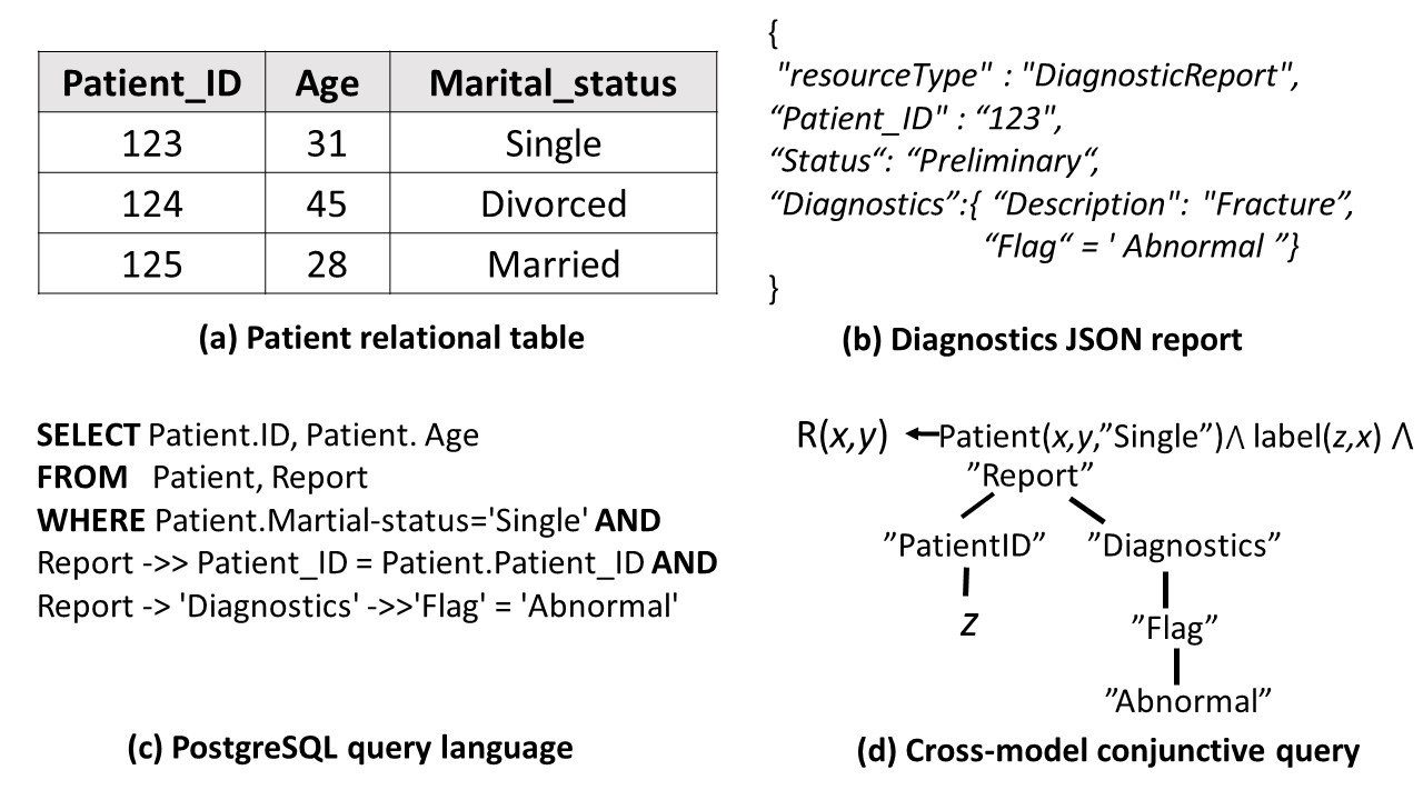
Figure 1: Illustration for the motivation and example of cross-model conjunctive query.

Example 1

Suppose we want to perform data analysis synergistically for heterogeneous medical records where the patient information is stored in a relational table and the diagnostic reports are formatted with JSON documents (See Figure 1). Assume that one query is to find the patient who is single and has an “abnormal” flag in the diagnostic report. Figure 1(c) illustrates the query language based on PostgreSQL database to perform the cross-model join between the relational table and the JSON document. This query can be naturally represented with a cross-model conjunctive query in Figure 1(d).

(a) A CMCQ

(b) Instances

(c) Result

Figure 2: An example of a CMCQ.

This paper embarks on the study of a Cross-Model Conjunctive Query (CMC Q) over both relations and trees. Figure 2 depicts a CMCQ. CMCQs emerge in modern data management and analysis, which often demands a hybrid evaluation with data organized in different formats and models, e.g. data lake [20], multi-model databases [26], polystores [13], and computational linguistics [38]. The detailed application scenarios of CMCQs can be exemplified as follows:

Data integration in data lake Data which resides in the data lake [20] may include highly structured data stored in SQL databases or data warehouses, and nesting or multiple values data in Parquet or JSON documents. Cross-model conjunctive queries on trees and relations can be used to integrate structured data from relational databases and semi-structured data in open data formats (e.g., through the PartiQL query language in Amazon Data lake [7]).

Cross-model query processing In the scenarios of multi-model databases [26] and polystores [13], query evaluation often involves data formatted with different models. The join problems between the structured and semi-structured data can boil down to evaluating a CMCQ over relations and trees.

Queries in computational linguistics A further area in which CMCQs are employed is computational linguistics, where one needs to search in, or check properties of large corpora of parsed natural language. Corpora such as Penn Treebank [38] are unranked trees labeled with the phrase structure of parsed texts. A conjunctive query on trees and relations can find sentences to satisfy specific semantic structure by relations (e.g. hyponym relations [37]) and corpora trees [41].

The number of applications that we have hinted at above motivates the study of CMCQs, and the main contributions of this paper are as follows:

1. This paper embarks on the study of the cross-model conjunctive query (CMC Q) and formally defines the problem of CMCQ processing, which integrates both relational conjunctive query and tree conjunctive pattern together.

2. We propose CMJoin-algorithm to process relations and encoded tree data efficiently. CMJoin produces worst-case optimal join result in terms of the label values as well as the encoded information values. In some cases, CMJoin is worst-case optimal join in the absence of encoded information.

3. Experiments on real-life and benchmark datasets show the effectiveness and efficiency of the algorithm in terms of running time and intermediate result size.

The remainder of the paper is organized as follows. In section 2 we provide preliminaries of approaches. We then extend the worst-case optimal algorithm for CMCQs in section 4. We evaluate our approaches empirically in section 5. We review related works in section 6. section 7 concludes the paper. Note that this is an extended version of previous work [9, 10, 11]

2 Preliminary

Cross-model conjunctive query Let $\mathbb{R}$ be a database schema and $R_{1},\ldots,$ $R_{n}$ be relation names in $\mathbb{R}$. A rule-based conjunctive query over $\mathbb{R}$ is an expression of the form $R_{0}(u_{0})\leftarrow R_{1}(u_{1})\wedge R_{2}(u_{2})\wedge\ldots\wedge R_{n}(u_{n})$, where $n\geq 0$, $R_{0}$ is a relation not in $\mathbb{R}$. Let $u_{0},u_{1},\ldots,u_{n}$ be free tuples, i.e. they may be either variables or constants. Each variable occurring in $u_{0}$ must also occur at least once in $u_{1},\ldots,u_{n}$.

Let $T$ be a tree pattern with two binary axis relations: Child and Descendant. The axis relations Child and Descendant are defined in the normal way [17]. In general, a cross-model conjunctive query contains three components: (i) the relational expression $\tau_{1}:=\exists r_{1},\ldots,r_{k}\colon R_{1}(u_{1})\wedge R_{2}(u_{2})\wedge\ldots\wedge R_{n}(u_{n})$, where $r_{1},\ldots,r_{k}$ are all the variables in the relations $R_{1},\ldots,R_{n}$; (ii) the tree expression $\tau_{2}:=\exists t_{1},\ldots,t_{k}\colon Child(v_{1})\wedge\ldots\wedge Descendant(v_{n})$, where $t_{1},\ldots,t_{k}$ are all the node variables occurring in $v_{i}$, for $i\geq 1$ and each $v_{i}$ is a binary tuple $(t_{i_{1}},t_{i_{2}})$; and (iii) the cross-model label expression $\tau_{3}:=\exists r_{1},\ldots,r_{k},t_{1},\ldots,t_{k}\colon label_{1}(t_{i_{1}},r_{j_{1}})\wedge\ldots\wedge label_{n}(t_{i_{n}},r_{j_{n}})$, where $\Sigma$ denotes a labeling alphabet. Given any node $t\in T$, $label(t,s)$ means that the label of the node $t$ is $s\in\Sigma$. The label relations bridge the expressions of relations and trees by the equivalence between the label values of the tree nodes and the values of relations.

By combining the three components together, we define a cross-model conjunctive query with the calculus of form $\left\{e_{1},\ldots,e_{m}\mid\tau_{1}\wedge\tau_{2}\wedge\tau_{3}\right\}$, where the variables $e_{1},\ldots,e_{m}$ are the return elements which occur at least once in relations.

(a) Conjunctive query form

(b) Simplified expression

Figure 3: Complete and simplified expressions of CMCQ

3(a) shows an example of a cross-model conjunctive query, which includes two relations and one tree pattern. For the purpose of expression simplicity, we do not explicitly distinguish between the variable of trees (e.g. $t_{a}$) and that of relations (e.g. $r_{a}$), but simply write them with one symbol (i.e. $a$) if $label(t_{a},r_{a})$ holds. We omit the label relation when it is clear from the context. 3(b) shows a simplified representation of a query.

Revisiting relational size bound We review the size bound for the relational model, which Asterias, Grohe, and Marx (AGM) [2] developed. The AGM bound is computed with linear programming (LP). Formally, given a relational schema $\mathbb{R}$, for every table $R\in\mathbb{R}$ let $A_{R}$ be the set of attributes of $R$ and $\mathcal{A}=\cup_{R}A_{R}$. Then the worst-case size bound is precisely the optimal solution for the following LP:

$$\underset{}{\text{maximize}} \Sigma^{\mathcal{A}}_{r}x_{r}$$ (3)

subject to $$\Sigma^{A_{R}}_{r}x_{r}\leq 1 \text{ for all }R\in\mathbb{R},$$

$$0\leq x_{r}\leq 1 \text{ for all }r\in\mathcal{A}.$$

Let $\rho$ denote the optimal solution of the above LP. Then the size bound of the query is $N^{\rho}$, where $N$ denotes the maximal size of each table. The AGM bound can be proved as a special case of the discrete version of the well-known Loomis-Whitney inequality [24] in geometry. Interested readers may refer to the details of the proof in [2]. We present these results informally and refer the readers to Ngo et al. [31] for a complete survey.

For example, we consider a typical triangle conjunctive query $R_{0}(a,b,c)\leftarrow R_{1}(a,b)\wedge R_{2}(b,c)\wedge R_{3}(a,c)$ that we introduced in section 1. Then the three LP inequalities corresponding to three relations include $x_{a}+x_{b}\leq 1$, $x_{b}+x_{c}\leq 1$, and $x_{a}+x_{c}\leq 1$. Therefore, the maximal value of $x_{a}+x_{b}+x_{c}$ is $3/2$, meaning that the size bound is $\mathcal{O}(N^{\frac{3}{2}})$. Interestingly, the similar case for CMCQ in Figure 7, the query $Q$ = $a[b]/c\bowtie R(b,c)$ has also the size bound $\mathcal{O}(N^{\frac{3}{2}})$.

3 Worst-case Size bound

Given a CMCQ $Q$, our analysis will be carried out in two assumptions: (1) regarding the tree database, given any label $s\in\Sigma$, the number of nodes with the label $s$ is at most $N$; (2) regarding the relational database, the size of each table is also at most $N$. Based on these two assumptions, we study how to find the maximum bound of the size of answers for $Q$ in the worst case. In this section, we start our investigation with two simple yet important special cases followed with a generalized algorithm and optimizations.

3.1 Glance at two special cases

(a) Descendant axes query

(b) Tree instance

(c) Child axes query

(d) Tree instance

Figure 4: Tree conjunctive queries with (a) Descendant axes and (c) Child axes, and their worst-case instance tree (b) for query (a) and tree (d) for query (c).

A cross-model query $Q$ include two components: relation expressions and tree patterns. As mentioned in section 2, the conditions of relational part can be captured through LP inequalities in the AGM bound. Now the key challenge is how to represent the tree structure with the inequalities. In fact, the most important component of our algorithms is a method to appropriately define LP inequality constraints for the tree pattern. To this end, we start our journey with two special cases, where the tree pattern contains only child or descendant axes, which shed light on the computation of a general case later.

Only descendant axes   When the tree pattern in $Q$ contains only descendant axes, it is a lucky fluke, thus there is no need to add any extra inequalities beside the existing relational inequalities. For example, consider a query $Q$ in 4(a) is a tree pattern. 4(b) shows an instance tree which realize the worst size bound. The result of $Q$ is $\mathcal{O}(N^{3})$ from all combination result of three nodes. Therefore, the existence of tree patterns with only descendant axes does not require any extra inequalities.

Only child axes   When the tree pattern in $Q$ contains only child axes, this case is different from the first one. For each path in the tree pattern, we need to add one parent-child (PC)-path inequality constraint. This is because each child node can have only one parent node to match the axis condition.

Definition 1 (PC-path inequality)

Let $P$ be a PC path in the tree pattern $\mathbf{T}$ and $A_{P}$ denote the set of labels of nodes in $P$. The PC-path inequality of $P$ is defined as $\Sigma^{A_{P}}_{r}x_{r}\leq 1$.

The matching result of attributes in a inequality is $\mathcal{O}(N)$ in relation as they are in one table and in PC-path, as they have one-to-one parent-child relationship. For example, see 4(c) for an example of query with only child axes. The pattern matching result of attribute ($a$,$b$,$c$) and ($a$,$d$) are both $\mathcal{O}(N)$. So, the PC-path inequalities are $x_{a}+x_{b}+x_{c}\leq 1$ and $x_{a}+x_{d}\leq 1$. The solution is 2 in this case, meaning that the result of $Q$ in 4(c) is $\mathcal{O}(N^{2})$. 4(d) shows one of the worst-case construction tree.

Mixed child and descendant axes   Given a tree pattern with both child and descendants axis relations, one may wonder whether the relational inequalities and PC-path inequalities are sufficient to produce the correct bound. Unfortunately, this situation is more complicated. The fact is that all relational and PC-path inequalities do not suffice to derive the correct bound, as illustrated below.

Example 2

Consider the query in 5(a) with only a tree pattern. The corresponding PC-path inequalities are $x_{a}+x_{b}\leq 1$, $x_{a}+x_{c}\leq 1$, and $x_{d}\leq 1$. Thus, the maximum value of $x_{a}+x_{b}+x_{c}+x_{d}$ is 3 when $x_{b}$=$x_{c}$=$x_{d}$=1 and $x_{a}$=0 (one of the possible solution). However, it is infeasible to construct a tree instance with $\Theta(N^{3})$ to match the result. In fact, the tight upper bound is only $\mathcal{O}(N^{2})$. 5(b) and 5(c) show two instances of trees in the worst case situation.

In this case, when we obtain $\mathcal{O}(N^{2})$ result for $b$ and $c$ in 5(b), $c$ and $d$ can not yield $\mathcal{O}(N^{2})$ result any more, meaning the $c$ and $d$ is no more equivalent to no constraint for descendant axe. And vice verse. So bound seems to be two alternatives: (i) $x_{a}+x_{b}\leq 1$, $x_{a}+x_{c}+x_{d}\leq 1$, and (ii) $x_{a}+x_{b}+x_{c}\leq 1$, $x_{d}\leq 1$, responding to two instance trees. They obtain the same size bound $\mathcal{O}(N^{2})$. These two different alternatives are meaningful to compute the size bound with more complex case. For example, give relation $R_{1}(b,c,d)$ (corresponding to $x_{b}+x_{c}+x_{d}\leq 1$), then with inequalities $(ii)$, it leads to the maximum bound $2$, while with the inequalities (i) it can obtain only $\frac{3}{2}$. For another example with relation $R_{3}(b,d)$ and $R_{4}(a,c,d)$ (corresponding to $x_{b}+x_{d}\leq 1$ and $x_{a}+x_{c}+x_{d}\leq 1$), this time with inequalities (i) is a winner with maximum value $2$, comparing to $\frac{3}{2}$ for the inequalities $(ii)$.

(a) Tree query

(b) Tree instance 1

(c) Tree instance 2

Figure 5: Tree conjunctive query (a) and its alternative worst-case instance tree (b) and tree (c).

Given a query with both ancestor and child axes, the above example hints at a possible approach to generate inequalities. That is, multiple options of LP problem settings need to be generated. In contrast to the AGM bound (with polynomial complexity), the computation of the size bound for a CMCQ is in general $\mathcal{NP}$-hard with respect to query complexity (i.e. the complexity is measured in the size of the query).

Theorem 3.1 (NP-hardness)

The query complexity of the worst-case bound evaluation of databases for a cross-model conjunctive query is $\mathcal{NP}$-hard.

The main idea of the proof is to polynomially reduce the 1-IN-3SAT problem [34] to our problem. See the Appendix in section 9 for the proof.

Remark   Note that this complexity is respect to the size of query. It should not be confused with the data complexity of query answering algorithm in section 4 later, which has polynomial complexity with respect to data complexity. Considering a practical size of a query is limited, from the point of view of applications, the above theorem mainly makes it of theoretical interest. In contrast to relational conjunctive queries that are tractable with respect to query complexity, this paper makes a contribution to demonstrate the theoretical complexity gap due to the occurrence of tree pattern in a conjunctive query.

3.2 Recursive conversion and split

This subsection develops a concrete algorithm to compute the worst-case bound. Here the high level idea is that we eliminate all descendant axis relations in the tree pattern recursively by two operations, called conversion and split, until the final tree pattern remains only child axis which can be solved through LP solutions. Then we acquire the size bound by picking the maximum solution for all generated LP problems.

Definition 2 (Conversion and split operations)

Let T be a tree pattern and $\alpha$ be a descendant axis between $x$ and $y$ nodes in T. Assume that $x$ is the parent of $y$.

1. Conversion: $T\mid\alpha$ denotes an operation to convert the descendant axis $\alpha$ to the child axis between $x$ and $y$.

2. Split: $T\parallel\alpha$ denotes an operation to remove $\alpha$ from $T$ and thereby $T$ is split into two subtrees. It is important to note that this split operation must be adjoined with one or multiple compensation inequalities defined below.

1

Input: A cross-model conjunctive query $Q$={$T,R$}

Output: Worst-case output size bound

2

$\mathbb{C}\leftarrow CP(T,\emptyset)$ ;

  // compute canonical suites

3 foreach  $(CT,CI)\in\mathbb{C}$ do

4       Generate the LP inequalities induced by $CT,CI$ and $R$

5       Solve the associated LP problem

6

7Return the maximum value for all solutions of LP problems

8

Algorithm 1 Computing bound

Definition 3 (Compensation inequalities)

With respective to the split operation in a tree pattern $T$, assume that node $x$ is split from node $y$. Let $P$ denote the root-to-$x$ path. For each root-to-leaf path $P^{\prime}$ that does not contain $x$, let $\mathbf{A}$ denote all labels in $P$ and $P^{\prime}$, then we generate a compensation inequality of $P^{\prime}$: $\Sigma x_{r}\leq 1$ for all labels $r\in\mathbf{A}$.

To understand the reason of compensation inequalities, recall the tree pattern in 2. When node $c$ is split from node $d$, a compensation inequality is emitted: $x_{a}+x_{b}+x_{c}\leq 1$. This is because due to the split of node $c$ and $d$ in the tree pattern, in the worst-case tree instance, each node $c$ should match each node $d$ (see Figure 5 c). Meanwhile, node $c$ must also have one parent node $a$ and this node $a$ must have at least one child $b$ node. Therefore, $x_{a}+x_{b}+x_{c}\leq 1$ is necessary to capture those structural constraints.

algorithm 1 illustrates the main steps to compute the bound. The input is a single tree pattern $T$ and relations $\mathbb{R}$. If there are multiple tree patterns, then we can easily merge them together by using a dummy root. The output is the value of the worst-case size bound. The key idea of this algorithm is to generate all canonical suites which can be converted to LP inequalities, as formally defined below.

Definition 4 (Suites and canonical suites)

A suite is a triple tuple ($\mathbb{R}$,$\mathbb{C}$,$\mathbb{T}$), where $\mathbb{R}$ denotes relations, $\mathbb{C}$ compensation inequalities and $\mathbb{T}$ tree patterns. In particular, we say one suite is canonical if all tree patterns in $\mathbb{T}$ contain only child axes. A canonical suite can be directly converted to a set of inequalities during the computation.

Given any canonical suite ($\mathbb{R}$,$\mathbb{C}$,$\mathbb{T}$), the LP problem setting can be generated as follows:

$$\underset{}{\text{maximize}} \Sigma^{\mathcal{A}}_{r}x_{r}$$ (4)

subject to $$\Sigma^{A_{R}}_{r}x_{r}\leq 1 for\ all\ R\in\mathbb{R}$$

$$\Sigma^{A_{P}}_{r}x_{r}\leq 1 for\ all\ P\in\mathbb{T}$$

$$\Sigma^{A_{C}}_{r}x_{r}\leq 1 for\ all\ C\in\mathbb{C}$$

$$0\leq x_{r}\leq 1 for\ all\ r\in\mathcal{A}$$

1

Input: A tree pattern query $T$ and the associated compensation inequalities $CI$ and relations R

Output: A set of canonical suites $\mathbb{C}$

2

3if there exists any descendant axis in $T$ then

4       Let $\alpha$ be a highest descendant axis in $T$

       $T_{1}\leftarrow T\mid\alpha$ ;

        // tree conversion

5       $\mathbb{C}\leftarrow CS(T_{1},CI,R)$

       $T_{2},T_{3},CI\leftarrow T\parallel\alpha$ ;

        // tree split

6      

7      foreach  $(CT_{2},CI_{2},R)$ in $CS(T_{2},CI,R)$ do

8            foreach  $(CT_{3},CI_{3},R)$ in $CS(T_{3},CI,R)$ do

9                  $\mathbb{M}$ = $\mathbb{C}$ $\cup$ {$(CT_{2}\cup CT_{3},CI_{2}\cup CI_{3},R)$}

10            

11      return $\mathbb{C}$

12      

13else

14      return $\big{\{}(\{T\},CI,R)\big{\}}$

15

Algorithm 2 Find all canonical suites $CS(T,CI,R)$

algorithm 2 illustrates the procedure to generate all canonical suites. At a high level, the main idea is to traverse the query tree pattern $T$ in a top down fashion to recursively eliminate all descendant axes through split and conversion operations. Let us walk through the algorithm. If there is any descendant axis, then we pick a highest one $\alpha$, to which there is no descendant axis in the path from root. Line 3 performs conversion operation and Line 4 adds the generated suites to $\mathbb{C}$. Then Line 5 performs the conversion operation and Line 6-8 recursively call the functions to process subtrees which are generated from split operation. When there is no descendant axis, Line 11 returns the canonical suite.

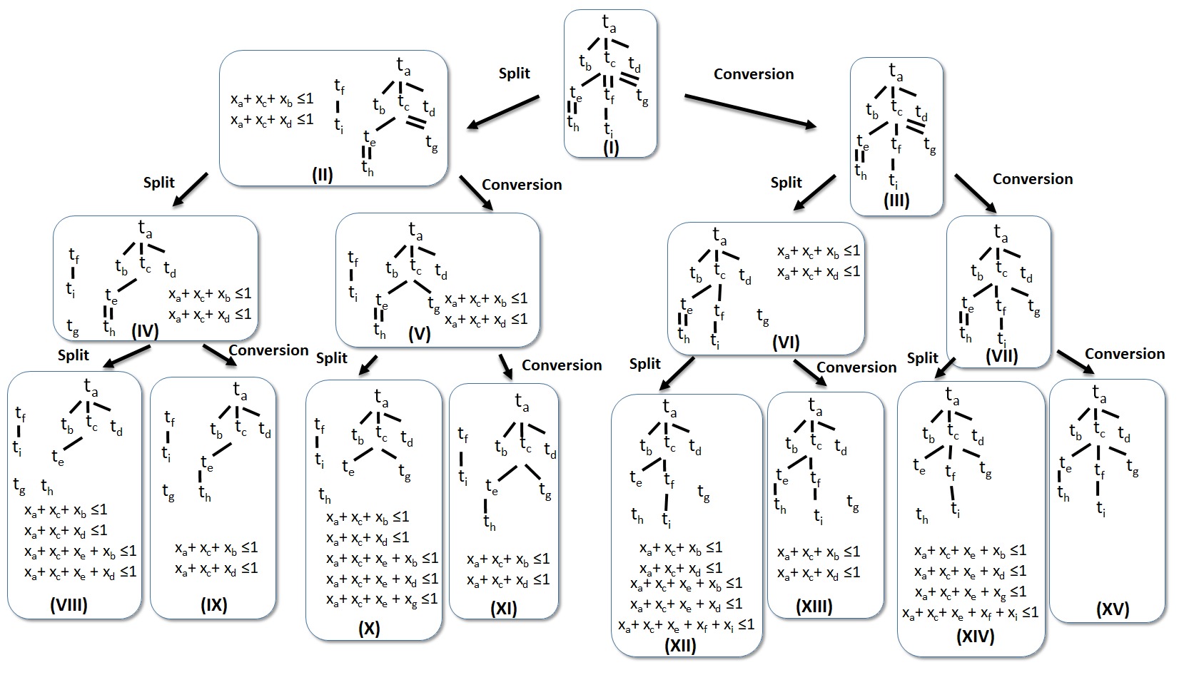
Figure 6: The tree query example for illustrating conversion and split.

Example 3

Figure 6 depicts the detailed procedure to process a cross-model query, where the tree query is shown in Figure 6(I) and the two relations are $R_{1}(a,c,e,h)$ and $R_{2}(h,g,i)$. Since $T$ has three descendant axes, Algorithm 2 generates eight ($2^{3}$) sets of canonical suites. Then those canonical suites are converted to LP inequalities in Algorithm 1. By solving all LP problems, the maximal value of bound is $\mathcal{O}(N^{5})$, where $x_{b}=x_{d}=x_{e}=x_{f}=x_{g}=1$. In particular, the max bound of each suite is shown as follows: suite (VIII) = 4, suite (IX) = 5, suite (X) = 4, suite (XI) = 5, suite (XII) = 4, suite (XIII) = 5, suite (XIV) = 4, and suite (XV) = 5,

Theorem 3.2

Our algorithm finds the correct size bound.

The proof can be found in the Appendix.

3.3 Two optimization rules

Given a tree pattern with $n$ descendant axes, the above algorithm needs to generate all $2^{n}$ canonical suites to find the maximum bound. Although in the worst case, this complexity nature cannot be alleviated if $NP\neq P$, this subsection proposes two rules to significantly reduce the search space in most cases to improve the efficiency.

Optimization 1: Given any single tree pattern $T$, assume that there is already a conversion operation performed on $T$, then we observe that any following split operations can be safely canceled without affecting the correctness of the computation. For example, recall Figure 6. We can safely stop the computation for all conversion operations after the split. That is, suites (X), (XII), (XIII) and (XIV) can be canceled. Note that although suite (XIII) generates the maximal value 5, this value can be also provided from other suites (e.g. from suites (IX) and (XI)).

Lemma 1

Given a single tree pattern $T$, the conversion operations in $T$ after the spit are avoidable without affecting the final result of worst-case bound.

The proof of 1 can be found in Appendix. Intuitively, this result holds because, to construct the worst case tree instance, a conversion operation requires the horizontal expansion of tree nodes, while a split operation demands the vertical expansion. The key observation is that the vertical expansion after the horizontal expansion cannot produce a new worst-case bound. Therefore, there is no need to carry out the conversion operation after the spit. Further, it is worthy to note that the above optimization can be applied only if the split and conversion operations are performed within the same tree. If the tree is split into two separated subtrees, then the split operation in the other subtree cannot be canceled.

Optimization 2: Given any descendant axis $\alpha$, if there is no more descendant axis under $\alpha$, then we call $\alpha$ a leaf descendant axis. We observe that, if the condition in 2 is satisfied, then the split operation for $\alpha$ can be safely canceled.

Lemma 2

Given a leaf descendant axis $\alpha$ between node $x$ and $y$, assume that $A$ denotes all labels for the root-to-$y$ path, we define an inequality $\Sigma^{\mathcal{A}}_{r}x_{r}\leq 1$. If this inequality cannot change the maximum solution for the current LP problem, then the split operation in the leaf descendant axis can be safely canceled .

Recall Figure 6. We can safely avoid the computation for the suites (VIII), (X), (XII) and (XIV) based on 2. Combining the rule in Lemma 1 together, we compute only 3 suites out of a total of 8, significantly reducing the search space.

One might wonder why the second optimization would not be more aggressive to apply on all descendant axis. This is because this aggressive strategy cannot be combined with Optimization 1. For example, consider a path pattern “$a//b//c$”. If we perform a conversion operation between $a$ and $b$, then based on Optimization 1, we cannot do the split between $b$ and $c$, leading to a suboptimal solution. Therefore, in Optimization 2, we consider a conservative strategy for only leaf descendant axis.

4 Approach

In this section, we tackle the challenges in designing a worst-case optimal algorithm for CMCQs over relational and tree data. We briefly review the existing relational worst-case optimal join algorithms. We represent these results informally and refer the readers to Ngo et al. [31] for a complete survey. The first algorithm to have a running time matching these worst-case size bounds is the NPRR algorithm [30]. An important property in NPRR is to estimate the intermediate join size and avoid to produce the case which is larger than the worst-case bound. In fact, for any join query, its execution time can be upper bounded by the AGM [2]. Interestingly, LeapFrog [36] and Joen [12] completely abandon the “query plan” and propose to deal with one attribute at a time with multiple relations at the same time.

(a) Tree query $Q$

(b) Table $D_{R_{1}}$

(c) Encode Tree $D_{T}$

Figure 7: A CMCQ (a) and its table instance (b) and tree instance (c).

4.1 Tree and relational data representation

To answer a tree pattern query, a positional representation of occurrences of tree elements and string values in the tree database are widely used, which extends the classic inverted index data structure in information retrieval. There existed two common ways to encode an instance tree, i.e. Dewey encoding [27] and containment encoding [6]. These decodings are necessary as they allow us to partially join tree patterns to avoid undesired intermediate result. After encoding, each attribute $j$ in the query node can be represented as a node table in form of $t_{j}(r_{j},p_{j})$, where $r_{j}$ and $p_{j}$ are the label value and position value, respectively. Check an example from a encoded tree instance in 7(c). The position value can be added in $\mathcal{O}(N)$ by one scan of the original tree. Note that we use Dewey coding in our implementation but the following algorithm is not limited to such representation. Any representation scheme which captures the structure of trees such as a region encoding [6] and an extended Dewey encoding [27] can all be applied in the algorithm.

All the data in relational are label data, and all relation tables and node tables will be expressed by the Trie index structure, which is commonly applied in the relational worst-case optimal algorithms (e.g. [1, 36]). The Trie structure can be accomplished using standard data structures (notably, balanced trees with $\mathcal{O}(\log n)$ look-up time or nested hashed tables with $\mathcal{O}(1)$ look-up time).

4.2 Challenges

In our context, tree data and twig pattern matching do make situation more complex. Firstly, directly materializing tree pattern matching may yield asymptotically more intermediate results. If we ignore the pattern, we may loose some bound constraints. Secondly, since tree data are representing both label and position values, position value joining may require more computation cost for pattern matching while we do not need position values in our final result.

Example 4

Recall that a triangle relational join query $Q$=$R_{1}(r_{a},r_{b})\bowtie R_{2}(r_{a},r_{c})$ $\bowtie R_{3}(r_{b},r_{c})$ has size bound $\mathcal{O}(N^{\frac{3}{2}})$. Figure 7 depicts an example of a CMCQ $Q$ with the table $R_{1}(r_{b},r_{c})$ and twig query $a[b]/c$ to return result $R_{0}(r_{a},r_{b},r_{c})$, which also has size bound $\mathcal{O}(N^{\frac{3}{2}})$ since the PC paths $a/b$ and $a/c$ are equivalent to the constraints $x_{a}+x_{b}\leq 1$ and $x_{a}+x_{c}\leq 1$, respectively. 7(b) and 7(c) show the instance table $D_{R_{1}}$ and the encoded tree $D_{T}$. The number of label values in the result $R_{0}(r_{a},r_{b},r_{c})$ is only $4$ rows which is $\mathcal{O}(N)$. On the other hand, the result size of only the tree pattern is $16$ rows which is $\mathcal{O}(N^{2})$, where $N$ is a table size or a node size for each attribute. The final result with the position values is also $\mathcal{O}(N^{2})$. Here, $\mathcal{O}(N^{2})$ is from the matching result of the position values of the attributes $t_{b}$ and $t_{c}$.

EmptyHeaded [1] applied the existing worst-case optimal algorithms to process the graph edge pattern matching. We may also attempt to solve relation-tree joins by representing the trees as relations with the node-position and the node-label tables and then reformulating the cross-model conjunctive query as a relational conjunctive query. However, as 4 illustrated, such method can not guarantee the worst-case optimality as extra computation is required for position value matching in a tree.

4.3 Cross-model join (CMJoin) algorithm

In this part, we discuss the algorithm to process both relational and tree data. As the position values are excluded in the result set while being required for the tree pattern matching, our algorithm carefully deals with it during the join. We propose an efficient cross-model join algorithm called CMJoin (cross-model join). In certain cases it guarantees the runtime optimality. We discover the join result size under three scenarios: with all node position values, with only branch node position value, and without position value.

Lemma 3

Given relational tables $\mathcal{R}$ and pattern queries $\mathcal{T}$, let $S_{r}$, $S_{p}$, and $S_{p}^{\prime}$ be the sets of all relation attributes, all position attributes, and only branch node position attributes, respectively. Then it holds that

$$\rho_{1}(S_{r}\cup S_{p})\geq\rho_{2}(S_{r}\cup S_{p}^{\prime})\geq\rho_{3}(S_{r}).$$ (5)

Proof

$Q(S_{r})$ is the projection result from $Q(S_{r}\cup S_{p}^{\prime})$ by removing all position values, and $Q(S_{r}\cup S_{p}^{\prime})$ is the projection result from $Q(S_{r}\cup S_{p})$ by removing non-branch position values. Therefore, the result size holds $\rho_{1}(S_{r}\cup S_{p})\geq\rho_{2}(S_{r}\cup S_{p}^{\prime})\geq\rho_{3}(S_{r})$.

Example 5

Recall the CMCQ $Q$ in 7(a), which is $Q$=$R_{1}(r_{b},r_{c})\bowtie a[b]/c$. Nodes $a$, $b$, $c$ in the tree pattern can be represented as node tables $(r_{a},p_{a})$, $(r_{b},p_{b})$, and $(r_{c},p_{c})$, respectively. So we have $Q(S_{r}\cup S_{p})=R(r_{a},r_{b},r_{c},p_{a},p_{b},p_{c})$, $Q(S_{r}\cup S_{p}^{\prime})=R(r_{a},r_{b},r_{c},p_{a})$, and $Q(S_{r})=R(r_{a},r_{b},r_{c})$. By the LP constraint bound for the relations and PC-paths, we achieve $\mathcal{O}(N^{2})$, $\mathcal{O}(N^{\frac{3}{2}})$, and $\mathcal{O}(N^{\frac{3}{2}})$ for the size bounds $\rho_{1}(S_{r}\cup S_{p})$, $\rho_{2}(S_{r}\cup S_{p}^{\prime})$, and $\rho_{3}(S_{r})$, respectively.

We elaborate CMJoin algorithm 3 more in the following. In the case of $\rho_{1}(S_{r}\cup S_{p})$=$\rho_{3}(S_{r})$, CMJoin executes a generic relational worst-case optimal join algorithm [1, 12] as the extra position values do not affect the worst-case final result. In other cases, CMJoin computes the path result of the tree pattern first. In this case, we project out all position values of a non-branch node for the query tree pattern. Then, we keep the position values of the only branch node so that we still can match the whole part of the tree pattern.

Input: Relational tables $\mathcal{R}$, pattern queries $\mathcal{T}$

$\mathcal{R}^{\prime}\leftarrow\emptyset$

  // Tree intermediate result

1

2if $\rho_{1}(S_{r}\cup S_{p})\leq\rho_{3}(S_{r})$ then // Theorem 4.1 condition (1)

3       foreach  $N\in\mathcal{T}$ do

             $\mathcal{R}^{\prime}\leftarrow\mathcal{R}^{\prime}\cup C_{N}(r_{N},p_{N})$

              // Nodes as tables

4            

5      

6else

7       $\mathcal{P}\leftarrow\mathcal{T}.getPaths()$

8       foreach  $P\in\mathcal{P}$ do

             $R_{P}(S_{r}\cup S_{p})\leftarrow$ path result of $P$

              // Paths as tables

9             $R_{P}^{\prime}(S_{r}\cup S_{p}^{\prime})\leftarrow$ project out non-branch position values of $R_{P}(S_{r}\cup S_{p})$

10             $\mathcal{R}^{\prime}\leftarrow\mathcal{R}^{\prime}\cup\{R_{P}^{\prime}(S_{r}\cup S_{p}^{\prime})\}$

11      

12

13$Q(S_{r}\cup S_{p}^{\prime})\leftarrow generic\_join(\mathcal{R}\cup\mathcal{R}^{\prime})$

14$Q(S_{r})\leftarrow$ project out all position values $Q(S_{r}\cup S_{p}^{\prime})$

Output: Join results $Q(S_{r})$

15

Algorithm 3 CMJoin

Theorem 4.1

Assume we have relations $\mathcal{R}$ and pattern queries $\mathcal{T}$. If either

1. $\rho_{1}(S_{r}\cup S_{p})\leq\rho_{3}(S_{r})$ or

2. (i) $\rho_{1}(S_{r}\cup S_{p}^{\prime})\leq\rho_{3}(S_{r})$ and (ii) for each path $P$ in $\mathcal{T}$ let $S_{r}^{\prime\prime}$ and $S_{p}^{\prime\prime}$ be the set of label and position attributes for $P$ so that $\rho_{4}(S_{r}^{\prime\prime}\cup S_{p}^{\prime\prime})\leq\rho_{3}(S_{r})$.

Then, CMJoin is worst-case optimal to $\rho_{3}(S_{r})$.

Proof

(1) Since the join result of the only label value $\rho_{3}(S_{r})$ is the projection of $\rho_{1}(S_{r}\cup S_{p})$, we can compute $Q(S_{r}\cup S_{p})$ first, then project out all the position value in linear of $\mathcal{O}(N^{\rho_{1}(S_{r}\cup S_{p})})$. Since $\rho_{1}(S_{r}\cup S_{p})\leq\rho_{3}(S_{r})$, we can estimate that the result size is limited by $\mathcal{O}(N^{\rho_{3}(S_{r})})$.

(2) $\rho_{1}(S_{r}^{\prime\prime}\cup S_{p}^{\prime\prime})\leq\rho_{3}(S_{r})$ means that each path result with label and position values are under worst-case result of $\rho_{3}(S_{r})$. We may first compute the path result and then project out all the non-branch position values. The inequality $\rho_{2}(r,p^{\prime})\leq\rho_{3}(r)$ means that the join result containing all branch position values has a worst-case result size which is still under $\rho_{3}(S_{r})$. Then by considering those position values as relational attribute values and by a generic relation join [30, 1], CMJoin is worst-case optimal to $\rho_{3}(S_{r})$.

Example 6

Recall the CMCQ query $Q=R_{1}(r_{b},r_{c})\bowtie a[b]/c$ in 7(a). Since $\rho_{1}(S_{r}\cup S_{p})>\rho_{3}(r)$, directly computing all label and position values may generate asymptotically bigger result ($\mathcal{O}(N^{2})$ in this case). So we can compute path results of $a/b$ and $a/c$, which are $(r_{a},p_{a},r_{b},p_{b})$ and $(r_{a},p_{a},r_{c},p_{c})$ and in $\mathcal{O}(N)$. Then we obtain only branch node results $(r_{a},p_{a},r_{b})$ and $(r_{a},p_{a},r_{c})$. By joining these project-out result with relation $R_{1}$ by a generic worst-case optimal algorithm, we can guarantee the size bound is $\mathcal{O}(N^{\frac{3}{2}})$.

Table 1: Intermediate result size ($10^{6}$) and running time (S) for queries. “/” and “-” indicate “timeout” ($\geq$ 10 mins) and “out of memory”. We measure the intermediate size by accumulating all intermediate and final join results.

	Intermediate result size($10^{6}$)					Running time (second)
Query	PG	SJ	VJ	EH	CMJoin	PG	SJ	VJ	EH	CMJoin
Q1	7.87x	2.60x	2.00x	1.68x	0.15	18.02x	1.39x	1.51x	1.66x	3.22
Q2	/	-	3.75x	4.83x	0.08	/	-	4.52x	129x	1.96
Q3	86.0x	62.6x	3.63x	4.61x	0.08	21.3x	4.27x	1.99x	4.28x	3.06
Q4	/	1.96x	1.75x	1.64x	0.24	/	2.34x	2.63x	1.82x	3.55
Q5	/	-	1.86x	1.77x	0.22	/	-	4.75x	39.8x	3.11
Q6	/	2.24x	2.00x	1.85x	0.21	/	6.10x	3.30x	2.89x	3.00
Q7	133x	106x	-	35.1x	0.29	4.82x	9.05x	-	7.18x	8.36
Q8	350x	279.8x	-	/	0.11	4.36x	5.61x	-	/	13.8
Q9	8.87x	8.34x	-	2.01x	4.62	1.12x	2.13x	-	1.48x	35.0
Q10	110x	440x	4.86x	/	0.07	2.91x	12.7x	1.22x	/	5.62
Q11	110x	440x	4.86x	/	0.07	2.11x	10.5x	0.88x	/	6.84
Q12	110x	440x	4.86x	/	0.07	2.68x	9.99x	1.06x	/	7.25
Q13	1.04x	1.22x	1.22x	1.07x	43.2	1.37x	4.81x	4.79x	1.31x	34.2
Q14	19.7x	2.56x	2.56x	3.90x	0.39	2.04x	3.82x	3.79x	2.14x	2.73
Q15	14.2x	1.85x	1.85x	17.0x	0.54	1.68x	3.53x	3.54x	2.01x	2.87
Q16	1.24x	1.24x	6.81x	2.15x	0.37	2.88x	1.32x	1.96x	1.02x	12.9
Q17	1.59x	7.84x	2.28x	1.31x	0.32	7.03x	3.58x	3.38x	2.10x	5.08
Q18	1.59x	7.13x	1.59x	1.64x	0.32	14.1x	5.21x	5.02x	2.06x	2.98
Q19	/	5.47x	6.62x	1.77x	0.45	/	1.41x	1.94x	0.89x	14.7
Q20	7.80x	25.1x	7.30x	4.19x	0.10	12.1x	6.77x	6.39x	3.17x	3.37
Q21	12.0x	36.1x	18.4x	14.7x	0.10	14.6x	8.82x	8.75x	10.9x	2.89
Q22	1.00x	18.5x	18.5x	0.96x	0.57	1.16x	5.22x	4.31x	2.35x	12.7
Q23	18.5x	18.5x	18.5x	1.61x	0.57	1.92x	2.17x	1.83x	1.02x	15.8
Q24	14.3x	3.02x	4.02x	0.96x	0.57	$>$9kx	$>$11kx	$>$12kx	0.18x	0.01
AVG	5.46x	5.90x	1.92x	1.90x	2.24	4.37x	5.34x	3.33x	3.46x	8.54

5 Evaluation

In this section, we experimentally evaluate the performance of the proposed algorithms and CMJoin with four real-life and benchmark data sets. We comprehensively evaluate CMJoin against state-of-the-art systems and algorithms concerning efficiency, scalability, and intermediate cost.

5.1 Evaluation setup

Datasets and query design Table 2 provides the statistics of datasets and designed CMCQs. These diverse datasets differ from each other in terms of the tree structure, data skewness, data size, and data model varieties. Accordingly, we designed 24 CMCQs to evaluate the efficiency, scalability, and cost performance of the CMJoin in various real-world scenarios.

Comparison systems and algorithms CMJoin is compared with two types of state-of-the-art cross-model solutions. The first solution is to use one query to retrieve a result without changing the nature of models [29, 40]. We implemented queries in PostgreSQL (PG), that supports cross-model joins. This enables the usage of the PG’s default query optimizer.

The second solution is to encode and retrieve tree nodes in a relational engine [5, 33, 42, 1]. We implemented two algorithms, i.e. structure join (SJ) (pattern matching first, then matching the between values) and value join (VJ) (label value matching first, then matching the position values). Also, we compared to a worst-case optimal relational engine called EmptyHeaded (EH) [1].

Experiment Setting We conducted all experiments on a 64-bit Windows machine with a 4-core Intel i7-4790 CPU at 3.6GHz, 16GB RAM, and 500GB HDD. We implemented all solutions, including CMJoin and the compared algorithms, in memory processing by Python 3. We measured the computation time of joining as the main metric excluding the time used for compilation, data loading, index presorting, and representation/index creation for all the systems and algorithms. We employed the Dewey encoding [27] in all experiments. The join order of attributes is greedily chosen based on the frequency of attributes. We measured the intermediate cost metric by accumulating all intermediate and final join results. For PG we accumulated all sub-query intermediate results. We repeated five experiments excluding the lowest and the highest measure and calculated the average of the results. Between each measurement of queries we wiped caches and re-loaded the data to avoid intermediate results.

Figure 8: Efficiency: runtime performance for all queries by $PG$, $SJ$, $VJ$, $EH$, and $CMJoin$. The performance time of more than 80s is cut for better presentation.

Efficiency Figure 8 shows the evaluation of the efficiency. In general, CMJoin is $3.33$-$13.43$ times faster in average than other solutions as shown in Table 1. These numbers are conservative as we exclude the “out of memory” (OOM) and “time out” (TO) results from the average calculation. Algorithms SJ, VJ, and EH perform relatively better compared to PG in the majority of the cases as they encoded the tree data into relation-like formats, making it faster to retrieve the tree nodes and match twig patterns.

Specifically in queries $Q1$-$Q6$, CMJoin, SJ, VJ, and EH perform better than PG, as the original tree is deeply recursive in the TreeBank dataset [38], and designed tree pattern queries are complex. So, it is costly to retrieve results directly from the original tree by PG. Instead, CMJoin, SJ, and VJ use encoded structural information to excel in retrieving nodes and matching tree patterns in such cases. In $Q2$ and $Q5$, EH performs worse. The reason is that it seeks for a better instance bound by joining partial tables and sub-twigs first and then aggregates the result. However, the separated joins yield more intermediate result in such cases in this dataset. In $Q1$ and $Q4$, which deal with a single table, SJ and VJ perform relatively close as no table joining occurs in these cases. However, in $Q2$-$Q3$ and $Q5$-$Q6$, SJ performs worse as joining two tables first leads to huge intermediate results in this dataset.

In contrast to the above, SJ outperforms VJ in $Q7$-$Q9$. The reason is that in the Xmark dataset [35], the tree data are flat and with less matching results in twig queries. The data in tables are also less skew. Therefore, SJ operates table joins and twig matching separately yielding relatively low results. Instead, VJ considers tree pattern matching later yielding too many intermediate results (see details of $Q7$ in Figure 9 and Figure 10) when joining label values between two models with non-uniform data. PG, which implements queries in a similar way of SJ, performs satisfactorily as well. The above comparisons show that compared solutions, which can achieve superiority only in some cases, and can not adapt well to dataset dynamics.

Queries $Q10$-$Q12$ have more complex tree pattern nodes involved. In these cases VJ filters more values and produces less intermediate results. Thus it outperforms SJ ($\sim$10x) and PG ($\sim$2x). For queries $Q10$-$Q12$ EH also yields huge intermediate results with more connections in attributes. The comparison between $Q7$-$Q9$ and $Q10$-$Q12$ indicates that the solutions can not adapt well to query dynamics.

Considering queries $Q13$-$Q15$ and $Q22$-$Q24$, PG performs relatively well since it involves only JSON and relational data. PG performs well in JSON retrieving because JSON documents have a simple structure. In $Q14$-$Q15$ most of the solutions perform reasonably well when the result size is small but SJ, and VJ still suffer from a large result size in $Q13$. With only JSON data, SJ and VJ perform similarly, as they both treat a simple JSON tree as one relation. In contrast in $Q16$-$Q21$, it involves XML, JSON and relational data from the UniBench dataset [40]. CMJoin, SJ, VJ, and EH perform better than PG. This is again because employing the encoding technique in trees accelerates node retrieval and matching tree patterns. Also, CMJoin, SJ, VJ, and EH are able to treat all the data models together instead of achieving results separately from each model by queries in PG.

Though compared systems and algorithms possess their advantages of processing and matching data, they straightforwardly join without bounding intermediate results, thus achieving sub-optimal performance during joining. CMJoin is the clear winner against other solutions, as it can wisely join between models and between data to avoid unnecessary quadratic intermediate results.

Figure 9: Scalability: runtime performance of PG, SJ, VJ, EH, and CMJoin. The x-axis is the percentage of data size. “oom” and “to” stand for “out of memory” error and “timeout” ($\geq$ 10 mins), respectively.

Scalability Figure 9 shows the scalability evaluation. In most queries, CMJoin performs flatter scaling as data size increases because CMJoin is designed to control the unnecessary intermediate output.

As discussed, CMJoin, SJ, VJ, and EH outperform PG in most of the queries, as the encoding method of the algorithms speeds up the twig pattern matching especially when the documents or queries are complex. However, PG scales better when involving simpler documents (e.g. in $Q15$ and $Q23$) or simpler queries (e.g. in $Q7$). Comparing to processing XML tree pattern queries, PG processes JSON data more efficiently.

Interestingly in $Q2$, SJ and PG join two relational tables separately from twig matching, generating quadratic intermediate results, thus leading to the OOM and TO, respectively. In $Q7$ VJ joins tables with node values without considering tree pattern structural matching and outputs an unwanted non-linear increase of intermediate results, thus leading to OOM in larger data size. Likewise evaluating EH between $Q2$ and $Q7$, it can not adapt well with different datasets. Performing differently in diverse datasets between SJ/PG and VJ/EH indicates that they can not smartly adapt to dataset dynamics. While increasing twig queries in $Q11$ compared to $Q7$, VJ filters more results and thus decreases the join cost and time in $Q11$. The comparison between SJ/EH and VJ shows dramatically different performance in the same dataset with different queries that indicates they can not smartly adapt to query dynamics.

In $Q11$, both CMJoin and VJ perform efficiently as they can filter out most of the values at the beginning. In this case, CMJoin runs slightly slower than VJ, which is reasonable as CMJoin maintains a tree structure whereas VJ keeps only tuple results. Overall, CMJoin judiciously joins between models and controls unwanted massive intermediate results. The evaluation shows that it performs efficiently and stably in dynamical datasets, with various queries and it also scales well.

Figure 10: Cost: intermediate result size. CM: CMJoin. JS: Joining step.

Cost analysis Table 1 presents the intermediate result sizes showing that CMJoin outputs 5.46x, 5.90x, 1.92x, and 1.90x less intermediate results on average than PG, SJ, VJ, and EH, respectively. Figure 10 depicts more detailed intermediate results for each joining step. In general, CMJoin generates less intermediate results due to its designed algorithmic process, worst-case optimality, as well as join order selections. In contrast, PG, SJ, and VJ can easily yield too many (often quadratic) intermediate results during joining in different datasets or queries. This is because they have no technique to avoid undesired massive intermediate results.

PG and SJ suffer when the twig matching becomes complex in datasets (e.g. $Q3$ and $Q10$), while VJ suffers in the opposite case of simpler twig pattern matching (e.g. $Q7$ and $Q16$). More specifically in $Q3$, PG and SJ output significant intermediate results by joining of two relational tables. In turn, VJ controls intermediate results utilizing the values of common attributes and tags between two models. On the other hand, in $Q7$, $Q9$, and $Q16$ VJ does not consider structural matching at first yielding unnecessary quadratic intermediate results. The above two-side examples indicate that solutions considering only one model at a time or joining values first without twig matching produce an undesired significant intermediate result.

EH suffers when the queries and attributes are more connected that leads to larger intermediate results during join procedures. The reason is that EH seeks a better instance bound so that it follows the query plan based on the GHD decomposition [1]. Our proposed method, CMJoin, by wisely joining between models, avoids an unnecessary massive intermediate output from un-joined attributes.

Summary We summarize evaluations of CMJoin as follows:

1. Extensive experiments on diverse datasets and queries show that averagely CMJoin achieves up to 13.43x faster runtime performance and produces up to 5.46x less intermediate results compared to other solutions.

2. With skew data CMJoin avoids undesired huge intermediate results by wisely joining data between models. With uniform data CMJoin filters out more values by joining one attribute at a time between all models.

3. With more tables, twigs, or common attributes involved CMJoin seems to perform more efficiently and scale better.

6 Related work

Worst-case size bounds and optimal algorithms Recently, Grohe and Marx [19] and Atserias, Grohe, and Marx [2] estimated size bounds for conjunctive joins using the fractional edge cover. That allows us to compute the worst-case size bound by linear programming. Based on this worst-case bound, several worst-case optimal algorithms have been proposed (e.g. NPRR [30], LeapFrog [36], Joen [12]). Ngo et al. [30] constructed the first algorithm whose running time is worst-case optimal for all natural join queries. Veldhuizen [36] proposed an optimal algorithm called LeapFrog which is efficient in practice to implement. Ciucanu et al. [12] proposed an optimal algorithm Joen which joins each attribute at a time via an improved tree representation. Besides, there exist research works on applying functional dependencies (FDs) for size bound estimation. The initiated study with FDs is from Gottlob, Lee, Valiant, and Valiant (GLVV) [18], which introduces an upper bound called GLVV-bound based on a solution of a linear program on polymatroids. The follow-up study by Gogacz et al. [15] provided a precise characterization of the worst-case bound with information theoretic entropy. Khamis et al. [23] provided a worst-case optimal algorithm for any query where the GLVV-bound is tight. See an excellent survey on the development of worst-case bound theory [31].

Multi-model data management As more businesses realized that data, in all forms and sizes, are critical to make the best possible decisions, we see a continuing growth of demands to manage and process massive volumes of different types of data [25]. The data are represented in various models and formats: structured, semi-structured, and unstructured. A traditional database typically handles only one data model. It is promising to develop a multi-model database to manage and process multiple data models against a single unified backend while meeting the increasing requirements for scalability and performance [25, 28]. Yet, it is challenging to process and optimize cross-model queries.

Previous work applied naive or no optimizations on (relational and tree) CMCQs. There exist two kinds of solutions. The first is to use one query to retrieve the result from the system without changing the nature of the model [29, 40]. The second is to encode and retrieve the tree data into a relational engine [1, 5, 33, 42]. Even though the second solution accelerates twig matching, they both may suffer from generating large, unnecessary intermediate results. These solutions or optimizations did not consider cross-model worst-case optimality. Some advances are already in development to process graph patterns [32, 21, 1]. In contrast to previous work, this paper initiates the study on the worst-case bound for cross-model conjunctive queries with both relation and tree structure data.

Join order In this paper, we do not focus on more complex query plan optimization. A better query plan [16, 14] may lead to a better bound for some instances [1] by combining the worst-case optimal algorithm and non-cyclic join optimal algorithm (i.e. Yannakakis [39]). We leave this as the future work to continue optimizing CMCQs.

Table 2: Dataset statistics and designed queries ($m$=$10^{6}$, $k$=$10^{3}$).

Dataset	Statistics	Query	Relational table	XML or JSON path query	LP	#Result
D1:TreeBank[38] (Linguistic data)	Zipfian Tables: 1$m$ rows XML: 2.4$m$ nodes	Q1	R1(NP,VP)	S[NP]/VP//PP[IN]//NNP	$N^{3}$	7.6$k$
		Q2	R1(NP,VP) R2(NP,PP)		$N^{3}$	4.6$k$
		Q3	R1(NP,VP) R3(NP,NNP)		$N^{3}$	¡0.1$k$
		Q4	R1(NP,VP)	S[NP]/VP//PP[IN]//NNP S/VP/PP/IN	$N^{3}$	1.4$k$
		Q5	R1(NP,VP) R2(NP,PP)		$N^{2}$	0.8$k$
		Q6	R1(NP,VP) R3(NP,NNP)		$N^{3}$	¡0.1$k$
D2:Xmark[35] (Auction data)	Normal Tables: 1$m$ rows XML: 1.6$m$ nodes	Q7	R1(incategory,quantity,email) R2(item,incategory,email) R3(item,quantity,email)	T7=Item[incategory]/quantity	$N^{2}$	91$k$
		Q8		T8=Item[incategory][localtion][quantity]//email	$N^{3}$	0.4$k$
		Q9		T9=Item[location]//email	$N^{3}$	2.4$m$
		Q10		T7, T8	$N^{3}$	0.7$k$
		Q11		T7, T9	$N^{3}$	0.7$k$
		Q12		T7, T8, T9	$N^{3}$	0.7$k$
D3:UniBench[40] (E-commerce)	Uniform Tables: 1$m$ rows JSON: 2$m$-4$m$ nodes	Q13	R1(asin,productID,orderID) R2(personID,lastname) R3(productID,product_info)	$.[orderID,personID]	$N^{3}$	37.0$m$
		Q14		$.[orderID,personID,orderline[productID]]	$N^{3}$	¡0.1$k$
		Q15		$.[personID,orderline[productID, asin]]	$N^{3}$	0.1$k$
D3:UniBench[40] (E-commerce)	Uniform Tables: 1$m$ rows JSON: 4$m$ nodes XML: 1.4$m$ nodes	Q16	R1(asin,orderID) R2(personID,lastname) $.[orderID,personID,orderline[asin]]	OrderLine[asin]/price	$N^{3}$	1.1$k$
		Q17		T17=Invoice[orderID]/orderline[asin]/price	$N^{3}$	¡0.1$k$
		Q18		T18=Invoice[orderID]//asin	$N^{3}$	¡0.1$k$
		Q19		orderline/asin, orderline/price	$N^{3}$	1.1$k$
		Q20		Invoice(I)/orderID, I/orderline(O)/asin, I/O/price	$N^{3}$	¡0.1$k$
		Q21		T17, T18	$N^{3}$	¡0.1$k$
D4:MIMIC-III[22] (Clinical data)	Uniform Tables:0.5-10$m$ rows JSON: 10$m$ nodes	Q22	R1(RowID,ICUstayID,ItemID,CGID), R2(RowID,SubjectID,ICUstayID,ItemID)	T22=$.[RowID,SubjectID,HADMID]	$N$	¡0.1$k$
		Q23	R1,R3(SubjectID,ItemID)	T22	$N^{\frac{3}{2}}$	¡0.1$k$
		Q24	R1,R2,R4(RowID,SubjectID,HADMID)	T22, T23=$.[RowID,ICUstayID,ItemID,CGID], T24=$.[RowID,SubjectID,HADMID,ICUstayID,ItemID,CGID]	$N$	¡0.1$k$

7 Conclusion and future work

In this paper, we studied the problems to find the worst-case size bound and optimal algorithm for cross-model conjunctive queries with relation and tree structured data. We provide the optimized algorithm, i.e. CMJoin, to compute the worst-case bound and the worst-case optimal algorithm for cross-model joins. Our experimental results demonstrate the superiority of proposal algorithms against state-of-the-art systems and algorithms in terms of efficiency, scalability, and intermediate cost. Exciting follow-ups will focus on adding graph structured data into our problem setting and designing a more general cross-model algorithm involving three data models, i.e. relation, tree and graph.

8 Acknowledgment

This paper is partially supported by Finnish Academy Project 310321 and Oracle ERO gift funding.

9 Appendix

Proof (of Theorem 3.1)

The proof idea is to polynomially reduce the 1-IN-3SAT problem [34] to our problem. The goal is to show that once we find the size bound of the query, we achieve the solution for 1-IN-3SAT. We briefly exploit the 1-in-3SAT problem in this part:

• Instance: A collection of clauses $l_{1}$, …, $l_{m}$, $m>$ 1; each $l_{i}$ is a disjunction of exactly three literals.

• Question: Is there a truth assignment to the variables occurring so that exactly one literal is true in each $l_{i}$?

Query construction functions: First, we introduce the basic functions for the proof as follows:

• $\mathcal{K}_{1}((A,B),(C,D))$ constructs a tree pattern query $T=A[C]/D[B]$ and two relations $R_{1}(B,C)$ and $R_{2}(B,D)$, i.e., $\mathcal{K}_{1}=T\bowtie R_{1}\bowtie R_{2}$;

• $\mathcal{K}_{2}((A,B),(C,D,E,F)$ constructs a tree pattern query $T=D[A]/F/B//C/E$ and three relations $R_{1}(A,F)$, $R_{2}(A,C,E)$, and $R_{3}(B,C,E)$, i.e., $\mathcal{K}_{2}=T\bowtie R_{1}\bowtie R_{2}\bowtie R_{3}$;

Polynomial Construction Given any 1-IN-3SAT input $\phi$ with $m$ clauses $\mathcal{L}=\{l_{1},...l_{i}...l_{m}\}$, where each $l_{i}$ is with $3$ variables, we create tree pattern and relation query set $\mathcal{Q}_{\phi}$, which is constructed as follows:

(1) Variable construction: In each clause $l_{i}$, for each variable in positive literal $x_{j}$, we establish two variables $x_{ij}$ and $a_{ij}$, while for its negative literal $\neg x_{j}$, we establish $y_{ij}$ and $b_{ij}$.

(2) Within clause restriction: For variable $x_{ik}$, $x_{ip}$, and $x_{id}$ in clause $l_{i}$, the construction form for each $l_{i}$ is following:

$$\mathcal{Q}_{1}=\mathcal{K}_{2}((x_{ik},a_{ik}),(x_{ip},a_{ip},x_{id},a_{id}))\bowtie$$ (6)

$$\mathcal{K}_{2}((x_{ip},a_{ip}),(x_{ik},a_{ik},x_{id},a_{id}))\bowtie$$

$$\mathcal{K}_{2}((x_{id},a_{id}),(x_{ik},a_{ik},x_{ip},a_{ip}))$$

(3) Variable restriction: For each variable’s positive literal $x_{k}$ in $l_{i}$ and its negative literal $\neg x_{k}$ in $l_{j}$, the construction form is as follows:

$$\mathcal{Q}_{2}=\mathcal{K}_{1}((x_{ik},a_{ik}),(y_{jk},b_{jk}))$$ (7)

(4) Between clauses restriction: For each two clauses $l_{i}=\{x_{ik},x_{ip},x_{id}\}$ and $l_{j}=\{\neg x_{jk},x_{jt},x_{jc}\}$ with same variable $x_{j}$ but in form of both positive and negative literals, the restrictions are constructed as follows:

$$\mathcal{Q}_{3}=\mathcal{K}_{2}((x_{ip},a_{ip}),(x_{jt},a_{jt},x_{jc},a_{jc}))\bowtie$$ (8)

$$\mathcal{K}_{2}((x_{id},a_{id}),(x_{jt},a_{jt},x_{jc},a_{jc}))\bowtie$$

$$\mathcal{K}_{2}((x_{jt},a_{jt}),(x_{ip},a_{ip},x_{id},a_{id}))\bowtie$$

$$\mathcal{K}_{2}((x_{jc},a_{jc}),(x_{ip},a_{ip},x_{id},a_{id}))$$

Table 3: Example of reduction from a 1-IN-3SAT instance to a CMCQ.

$\phi$	$(x_{1}\vee\neg x_{2}\vee x_{3})$	$(\neg x_{1}\vee x_{2}\vee x_{3})$	$(\neg x_{1}\vee x_{4}\vee x_{5})$	Description
$\mathcal{Q}_{1}$	$\begin{aligned} \mathcal{K}_{2}((x_{11},a_{11}),(y_{12},b_{12},x_{13},a_{13}))\\ \mathcal{K}_{2}((y_{12},b_{12}),(x_{11},a_{11},x_{13},a_{13}))\\ \mathcal{K}_{2}((x_{13},a_{13}),(x_{11},a_{11},y_{12},b_{12}))\end{aligned}$	$\begin{aligned} \mathcal{K}_{2}((y_{21},b_{21}),(x_{22},a_{22},x_{23},a_{23}))\\ \mathcal{K}_{2}((x_{22},a_{22}),(y_{21},b_{21},x_{23},a_{23}))\\ \mathcal{K}_{2}((x_{23},a_{23}),(y_{21},b_{21},x_{22},a_{22}))\end{aligned}$	$\begin{aligned} \mathcal{K}_{2}((y_{31},b_{31}),(x_{34},a_{34},x_{35},a_{35}))\\ \mathcal{K}_{2}((x_{34},a_{34}),(y_{31},b_{31},x_{35},a_{35}))\\ \mathcal{K}_{2}((x_{35},a_{35}),(y_{31},b_{31},x_{34},a_{34}))\end{aligned}$	One of $x_{j}$, $x_{d}$, $x_{p}$ in each clause $l_{i}$ is $True$
$\mathcal{Q}_{2}$	$\begin{aligned} \mathcal{K}_{1}((x_{11},a_{11}),(y_{21},b_{21})\\ \mathcal{K}_{1}((x_{11},a_{11}),(y_{31},b_{31})\end{aligned}$	$\begin{aligned} \mathcal{K}_{1}((x_{22},a_{22}),(y_{12},b_{12})\end{aligned}$		$x_{i}$ and $\neg x_{i}$ cannot be both $True$
$\mathcal{Q}_{3}$	$\begin{aligned} \mathcal{K}_{2}((y_{12},b_{12}),(x_{22},a_{22},x_{23},a_{23}))\\ \mathcal{K}_{2}((x_{13},a_{13}),(x_{22},a_{22},x_{23},a_{23}))\\ \mathcal{K}_{2}((y_{12},b_{12}),(x_{34},a_{34},x_{35},a_{35}))\\ \mathcal{K}_{2}((x_{13},a_{13}),(x_{34},a_{34},x_{35},a_{35}))\\ \end{aligned}$	$\begin{aligned} \mathcal{K}_{2}((x_{22},a_{22}),(y_{12},b_{12},x_{13},a_{13}))\\ \mathcal{K}_{2}((x_{23},a_{23}),(y_{12},b_{12},x_{13},a_{13}))\\ \mathcal{K}_{2}((y_{21},b_{21}),(x_{11},a_{11},x_{13},a_{13}))\\ \mathcal{K}_{2}((x_{23},a_{23}),(x_{11},a_{11},x_{13},a_{13}))\end{aligned}$	$\begin{aligned} \mathcal{K}_{2}((x_{34},a_{34}),(y_{12},b_{12},x_{13},a_{13}))\\ \mathcal{K}_{2}((x_{35},a_{35}),(y_{12},b_{12},x_{13},a_{13}))\end{aligned}$	$x_{i}$ and $\neg x_{i}$ cannot be both $False$

Therefore, $\mathcal{Q}_{\phi}=\mathcal{Q}_{1}\bowtie,\mathcal{Q}_{2}\bowtie\mathcal{Q}_{3}$. For $\mathcal{Q}_{\phi}$ construction, we establish $2*m$ variables, which is $\mathcal{O}(m)$. For each clause in $\mathcal{Q}_{1}$, we call three times of $\mathcal{K}_{2}()$ function, with each of $14$ elements of variables. So the construction cost is $3*m*14$, which is $\mathcal{O}(m)$. For variable in $\mathcal{Q}_{2}$, we call one time of $\mathcal{K}_{1}()$ for each variable with both positive and negative literals. In worst case, each positive literal has a negative literals, then the construction cost is at most $8*(3*m/2)^{2}$, which is $\mathcal{O}(m^{2})$. For each variable in $\mathcal{Q}_{3}$, the construction cost is linear (4 times, i.e., two variables to two variables) to $\mathcal{Q}_{2}$, i.e., $4*8*(3*m/2)^{2}$, which is $\mathcal{O}(m^{2})$. So the total construction cost is $\mathcal{O}(m^{2})$, which is a polynomial transformation. Note that we can replace relation tables by PC paths so that the CMCQ has only tree pattern queries.

Next, we introduce lemmas for the $\mathcal{K}_{1}()$ and $\mathcal{K}_{2}()$ functions as the proof foundation. Figure 11 shows an example to illustrate the $\mathcal{K}_{1}()$ and Figure 12 shows an example to illustrate the $\mathcal{K}_{2}()$ function and how it relates to $\phi$ instance.

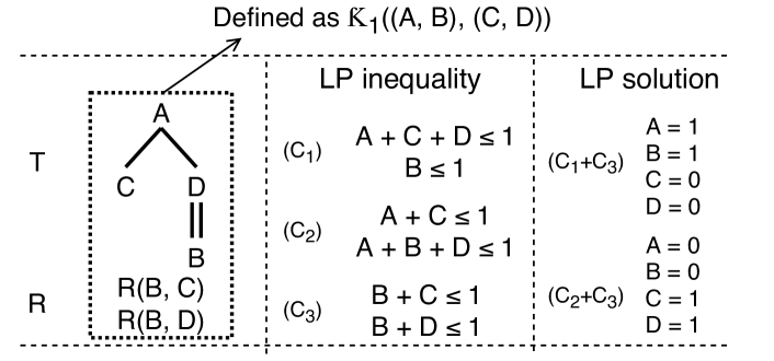
Figure 11: Illustration example for 4

Lemma 4

Given a tree pattern query $T=A[C]/D[B]$ and two relations $R_{1}(B,C)$ and $R_{2}(B,D)$, size bound $\Theta(N^{2})$ is obtained for $|Q=T\bowtie R_{1}\bowtie R_{2}|$ by constructing either $|A|=|B|=\Theta(N)$ or $|A|=|B|=\mathcal{O}(1)$.

Proof

First, $T$ can be equivalently transformed into two alternative constraint sets $C_{1}=\{(A,C,D),(B)\}$ and $C_{2}=\{(A,C),(B,C,D)\}$, i.e., $C_{1}:\{A+C+D\leq 1;~{}B\leq 1\}$ and $C_{2}:\{A+C\leq 1;~{}B+C+D\leq 1\}$ in LP form. And $R_{1}$ and $R_{2}$ is equivalent to $C_{3}=\{(B,C),(B,D)\}$, i.e., $C_{3}:\{B+C\leq 1;~{}B+D\leq 1\}$. The final size bound $\Theta(N^{2})$ is obtained by either $C_{1}\cup C_{3}$ or $C_{2}\cup C_{3}$, with LP solution $A=B=1$ or $A=B=0$ ($C=D=1$), respectively. In $C_{1}\cup C_{3}$, by combining $A+C+D\leq 1$ with $B+C\leq 1$ (or $B+D\leq 1$), we have $A+B+2C+D\leq 2$ (or $A+B+C+2D\leq 2$). If $C>0$ (or $D>0$), then $A+B+C+D<2$, meaning $Q$ can not achieve $\Theta(N^{2})$. Thus $C=D=0$, meaning $A=B=1$. Likewise in $C_{2}\cup C_{3}$, we obtain $A=B=0;~{}C=D=1$.

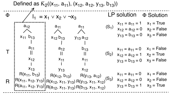
Figure 12: Illustration example for 5 and the query construction for a single clause.

Lemma 5

Given a tree pattern query $T=D[A]/F/B//C/E$ and three relations $R_{1}(A,F)$, $R_{2}(A,C,E)$, and $R_{3}(B,C,E)$, size bound $\Theta(N^{2})$ is obtained for $|Q=T\bowtie R_{1}\bowtie R_{2}\bowtie R_{3}|$ by constructing either $|A|=|B|=\Theta(N)$ or $|A|=|B|=\mathcal{O}(1)$.

Proof

First, $T$ can be transformed into two alternative inequality sets i.e., $C_{1}:\{A+B+D+F\leq 1;~{}C+E\leq 1\}$ and $C_{2}:\{A+D\leq 1;~{}B+C+D+E+F\leq 1\}$. And $R_{1}$, $R_{2}$, and $R_{2}$ is equivalent to $C_{3}:\{A+F\leq 1;~{}A+C+E\leq 1;~{}B+C+E\leq 1\}$. The final size bound $\Theta(N^{2})$ is obtained by either $C_{1}\cup C_{3}$ or $C_{2}\cup C_{3}$, with LP solution $A=B=1$ or $A=B=0$, respectively. In $C_{1}\cup C_{3}$, by combining $A+B+D+F\leq 1$ and $A+C+E\leq 1$, we have $2A+B+C+D+E+F\leq 2$, so $A$ should be $0$ to achieve final result $2$. By combining $A+B+D+F\leq 1$ and $B+C+E\leq 1$, we achieve $B=0$. Thus $A=B=0$ achieves $\mathcal{O}(N^{2})$ in this case. While in $C_{2}\cup C_{3}$, combining $B+C+D+E+F\leq 1$ with $A+D\leq 1$, $A+F\leq 1$, and $A+C+E\leq 1$, we obtain $D=0$, $F=0$ and $C=E=0$, respectively. Thus $A=B=1$ achieves $\Theta(N^{2})$.

We now prove that $\mathcal{Q}_{\phi}$ achieves size bound $\Theta(N^{2m})$ if and only if $\phi$ is satisfiable, where $m$ is number of clause.

(1) If we achieve $\Theta(N^{2m})$ size bound for $\mathcal{Q}_{\phi}$, then we can achieve $\Theta(N^{2})$ for each clause. By within clause restriction $\mathcal{Q}_{1}$, for variable $x_{ij}$, $x_{ip}$, and $x_{id}$ in clause $l_{i}$, only one of $x_{ij}=a_{ij}$, $x_{ip}=a_{ip}$, and $x_{id}=a_{id}$ is assigned to be $1$ to achieve size bound $\Theta(N^{2})$, corresponding to only one of $x_{j}$, $x_{p}$, or $x_{d}$ in each clause $l_{i}$ to be assigned to be $True$. By $\mathcal{Q}_{2}$ for each variable $x_{k}$, by 4, either $x_{ik}=a_{ik}=1$ or $y_{jk}=b_{jk}=1$, corresponding to $x_{i}=True$ or $\neg x_{i}=True$ in $\phi$, respectively, meaning that $x_{k}$ and $\neg x_{k}$ can not be both $True$. By $\mathcal{Q}_{3}$ for each two clauses $l_{i}=\{x_{ik},x_{ip},x_{id}\}$ and $l_{j}=\{\neg x_{jk},x_{jt},x_{jc}\}$ with common variable $x_{k}$ in different (one positive and one negative) literal forms, $\mathcal{Q}_{3}$ guarantees, if $x_{ik}=a_{ik}=0$, then $x_{ip}=a_{ip}=1$ or $x_{id}=a_{id}=1$, which forces $x_{jt}=n_{jt}=0$ and $x_{jc}=n_{jc}=0$, thus making $y_{jk}=b_{jk}=1$. Likewise, when $y_{jk}=b_{jk}=0$, we have $x_{ik}=a_{ik}=1$. $\mathcal{Q}_{3}$ corresponds to property that $x_{j}$ and $\neg x_{j}$ can not be both $False$. By these assignments, each clause is with one $True$, and each variable pair $x_{k}$ and $\neg x_{k}$ can not be both $True$ and both $False$, then $\phi$ is satisfiable.

(2) Conversely, if $\phi$ is satisfiable, then we have only one $True$ variable in one of $x_{j}$, $x_{p}$, or $x_{d}$ in each clause $l_{i}$. We can assign LP values to corresponding variables $x_{ij}=a_{ij}$, $x_{ip}=a_{ip}$, or $x_{id}=a_{id}$ in $\mathcal{Q}_{\phi}$ such that each clause achieve $\Theta(N^{2})$. Since each variable pair $x_{k}$ and $\neg x_{k}$ can not be both $True$ and both $False$. So assigning LP values satisfies our $\mathcal{Q}_{2}$ and $\mathcal{Q}_{3}$ constructions. By summing up $m$ clause results, we achieve $|\mathcal{Q}_{\phi}|=\Theta(N^{2m})$. By our construction, as each clause has $6$ variables and is with $\mathcal{O}(N^{2})$ by 5, meaning that $\mathcal{Q}_{\phi}$ is upper bounded by $\mathcal{O}(N^{2m})$. Therefore, we achieve the size bound of $\mathcal{Q}_{\phi}$.

Therefore, $\mathcal{Q}_{\phi}$ achieves the size bound $\Theta(N^{2m})$ if and only if $\phi$ is satisfiable.

Example 7

Table 3 shows a full example to illustrate the reduction from a 1-in-3SAT instance. Given $\phi$, we construct the tree pattern query and relation by our polynomial transformation.

We can achieve the size bound $\Theta(N^{(2*m)})$ = $\Theta(N^{6})$ by assigning $x_{11}=a_{11}=x_{22}=a_{22}=x_{34}=a_{34}=1$, where $m=3$ is the clause numbers. So the LP solution corresponds to the satisfiable solution for $\phi$, i.e., $x_{1}=True$, $x_{2}=False$, and $x_{3}=False$.

Conversely, satisfiable solution $x_{1}=True$, $x_{2}=False$, and $x_{3}=False$ in $\phi$ achieves size bound $\Theta(N^{6})$ by assigning $x_{11}=a_{11}=x_{22}=a_{22}=x_{34}=a_{34}=1$.

References

- [1] Christopher R. Aberger, Susan Tu, Kunle Olukotun, and Christopher Ré. Emptyheaded: A relational engine for graph processing. In SIGMOD Conference, pages 431–446. ACM, 2016.
- [2] Albert Atserias, Martin Grohe, and Dániel Marx. Size bounds and query plans for relational joins. In FOCS, pages 739–748. IEEE Computer Society, 2008.
- [3] Michael Benedikt, Wenfei Fan, and Gabriel Kuper. Structural properties of xpath fragments. Theoretical Computer Science, 336(1):3 – 31, 2005. Database Theory.
- [4] Henrik Björklund, Wim Martens, and Thomas Schwentick. Conjunctive query containment over trees. In Proceedings of the 11th International Conference on Database Programming Languages, DBPL’07, 2007.
- [5] Zakaria Bousalem and Ilias Cherti. Xmap: A novel approach to store and retrieve XML document in relational databases. JSW, 10(12):1389–1401, 2015.
- [6] Nicolas Bruno, Nick Koudas, and Divesh Srivastava. Holistic twig joins: optimal XML pattern matching. In SIGMOD Conference, pages 310–321. ACM, 2002.
- [7] Mengchu Cai, Martin Grund, Anurag Gupta, Fabian Nagel, Ippokratis Pandis, Yannis Papakonstantinou, and Michalis Petropoulos. Integrated querying of SQL database data and S3 data in amazon redshift. IEEE Data Eng. Bull., 41(2):82–90, 2018.
- [8] Surajit Chaudhuri and Moshe Y. Vardi. On the equivalence of recursive and nonrecursive datalog programs. In PODS, pages 55–66. ACM Press, 1992.
- [9] Yuxing Chen. Worst case optimal joins on relational and XML data. In SIGMOD Conference, pages 1833–1835. ACM, 2018.
- [10] Yuxing Chen. Performance tuning and query optimization for big data management. 2021.
- [11] Yuxing Chen, Valter Uotila, Jiaheng Lu, Zhen Hua Liu, and Souripriya Das. Cross-model conjunctive queries over relation and tree-structured data. In DASFAA (1), volume 13245 of Lecture Notes in Computer Science, pages 21–37. Springer, 2022.
- [12] Radu Ciucanu and Dan Olteanu. Worst-case optimal join at a time. Technical report, Technical report, Oxford, 2015.
- [13] Jennie Duggan, Aaron J. Elmore, Michael Stonebraker, Magdalena Balazinska, Bill Howe, Jeremy Kepner, Sam Madden, David Maier, Tim Mattson, and Stanley B. Zdonik. The bigdawg polystore system. SIGMOD Record, 44(2):11–16, 2015.
- [14] Wolfgang Fischl, Georg Gottlob, and Reinhard Pichler. General and fractional hypertree decompositions: Hard and easy cases. In PODS, pages 17–32. ACM, 2018.
- [15] Tomasz Gogacz and Szymon Toruńczyk. Entropy bounds for conjunctive queries with functional dependencies. arXiv preprint arXiv:1512.01808, 2015.
- [16] Georg Gottlob, Martin Grohe, Nysret Musliu, Marko Samer, and Francesco Scarcello. Hypertree decompositions: Structure, algorithms, and applications. In International Workshop on Graph-Theoretic Concepts in Computer Science, pages 1–15. Springer, 2005.
- [17] Georg Gottlob, Christoph Koch, and Klaus U. Schulz. Conjunctive queries over trees. J. ACM, 53(2):238–272, 2006.
- [18] Georg Gottlob, Stephanie Tien Lee, Gregory Valiant, and Paul Valiant. Size and treewidth bounds for conjunctive queries. J. ACM, 59(3):16:1–16:35, 2012.
- [19] Martin Grohe and Dániel Marx. Constraint solving via fractional edge covers. ACM Trans. Algorithms, 11(1), August 2014.
- [20] Rihan Hai, Sandra Geisler, and Christoph Quix. Constance: An intelligent data lake system. In SIGMOD Conference, pages 2097–2100. ACM, 2016.
- [21] Aidan Hogan, Cristian Riveros, Carlos Rojas, and Adrián Soto. A worst-case optimal join algorithm for SPARQL. In ISWC (1), volume 11778 of Lecture Notes in Computer Science, pages 258–275. Springer, 2019.
- [22] Alistair EW Johnson, Tom J Pollard, Lu Shen, H Lehman Li-wei, Mengling Feng, Mohammad Ghassemi, Benjamin Moody, Peter Szolovits, Leo Anthony Celi, and Roger G Mark. Mimic-iii, a freely accessible critical care database. Scientific data, 3:160035, 2016.
- [23] Mahmoud Abo Khamis, Hung Q. Ngo, and Dan Suciu. Computing join queries with functional dependencies. In PODS, pages 327–342. ACM, 2016.
- [24] Lynn H Loomis and Hassler Whitney. An inequality related to the isoperimetric inequality. Bulletin of the American Mathematical Society, 55(10):961–962, 1949.
- [25] Jiaheng Lu and Irena Holubová. Multi-model data management: What’s new and what’s next? In EDBT, pages 602–605. OpenProceedings.org, 2017.
- [26] Jiaheng Lu and Irena Holubová. Multi-model databases: A new journey to handle the variety of data. ACM Comput. Surv., 52(3):55:1–55:38, June 2019.
- [27] Jiaheng Lu, Tok Wang Ling, Chee Yong Chan, and Ting Chen. From region encoding to extended dewey: On efficient processing of XML twig pattern matching. In VLDB, pages 193–204. ACM, 2005.
- [28] Jiaheng Lu, Zhen Hua Liu, Pengfei Xu, and Chao Zhang. UDBMS: road to unification for multi-model data management. CoRR, abs/1612.08050, 2016.
- [29] Hassana Nassiri, Mustapha Machkour, and Mohamed Hachimi. One query to retrieve XML and relational data. In FNC/MobiSPC, volume 134 of Procedia Computer Science, pages 340–345. Elsevier, 2018.
- [30] Hung Q. Ngo, Ely Porat, Christopher Ré, and Atri Rudra. Worst-case optimal join algorithms. J. ACM, 65(3):16:1–16:40, March 2018.
- [31] Hung Q. Ngo, Christopher Ré, and Atri Rudra. Skew strikes back: new developments in the theory of join algorithms. SIGMOD Record, 42(4):5–16, 2013.
- [32] Dung T. Nguyen, Molham Aref, Martin Bravenboer, George Kollias, Hung Q. Ngo, Christopher Ré, and Atri Rudra. Join processing for graph patterns: An old dog with new tricks. In GRADES@SIGMOD/PODS, pages 2:1–2:8. ACM, 2015.
- [33] Amjad Qtaish and Kamsuriah Ahmad. Xancestor: An efficient mapping approach for storing and querying XML documents in relational database using path-based technique. Knowl.-Based Syst., 114:167–192, 2016.
- [34] Thomas J Schaefer. The complexity of satisfiability problems. In Proceedings of the tenth annual ACM symposium on Theory of computing, pages 216–226. ACM, 1978.
- [35] Albrecht Schmidt, Florian Waas, Martin L. Kersten, Michael J. Carey, Ioana Manolescu, and Ralph Busse. Xmark: A benchmark for XML data management. In VLDB, pages 974–985. Morgan Kaufmann, 2002.
- [36] Todd L Veldhuizen. Leapfrog triejoin: A simple, worst-case optimal join algorithm. arXiv preprint arXiv:1210.0481, 2012.
- [37] Bifan Wei, Jun Liu, Jian Ma, Qinghua Zheng, Wei Zhang, and Boqin Feng. Motif-based hyponym relation extraction from wikipedia hyperlinks. IEEE Trans. Knowl. Data Eng., 26(10):2507–2519, 2014.
- [38] Naiwen Xue, Fei Xia, Fu-Dong Chiou, and Marta Palmer. The penn chinese treebank: Phrase structure annotation of a large corpus. Natural language engineering, 11(2):207–238, 2005.
- [39] Mihalis Yannakakis. Algorithms for acyclic database schemes. In VLDB, pages 82–94. IEEE Computer Society, 1981.
- [40] Chao Zhang, Jiaheng Lu, Pengfei Xu, and Yuxing Chen. Unibench: A benchmark for multi-model database management systems. In Technology Conference on Performance Evaluation and Benchmarking, pages 7–23. Springer, 2018.
- [41] Junru Zhou and Hai Zhao. Head-driven phrase structure grammar parsing on Penn treebank. In Proceedings of the 57th Annual Meeting of the Association for Computational Linguistics, July 2019.
- [42] Huchao Zhu, Huiqun Yu, Guisheng Fan, and Huaiying Sun. Mini-xml: An efficient mapping approach between XML and relational database. In ICIS, pages 839–843. IEEE Computer Society, 2017.