Trajectory-dependent Generalization Bounds for Deep Neural Networks via Fractional Brownian Motion

Abstract

Despite being tremendously overparameterized, it is appreciated that deep neural networks trained by stochastic gradient descent (SGD) generalize surprisingly well. Based on the Rademacher complexity of a pre-specified hypothesis set, different norm-based generalization bounds have been developed to explain this phenomenon. However, recent studies suggest these bounds might be problematic as they increase with the training set size, which is contrary to empirical evidence. In this study, we argue that the hypothesis set SGD explores is trajectory-dependent and thus may provide a tighter bound over its Rademacher complexity. To this end, we characterize the SGD recursion via a stochastic differential equation by assuming the incurred stochastic gradient noise follows the fractional Brownian motion. We then identify the Rademacher complexity in terms of the covering numbers and relate it to the Hausdorff dimension of the optimization trajectory. By invoking the hypothesis set stability, we derive a novel generalization bound for deep neural networks. Extensive experiments demonstrate that it predicts well the generalization gap over several common experimental interventions. We further show that the Hurst parameter of the fractional Brownian motion is more informative than existing generalization indicators such as the power-law index and the upper Blumenthal-Getoor index.

Keywords: generalization bound, optimization trajectory, fractional Brownian motion, hypothesis set stability, stochastic gradient descent

1 Introduction

Over the past decade, deep neural networks (DNNs) have enjoyed remarkable success in many scientific fields. Despite suffering from serious overparameterization, they generalize surprisingly well. One point of view argues that this is due to the implicit regularization imposed via stochastic gradient descent (SGD) (Keskar et al., 2017; Barrett and Dherin, 2021; Smith et al., 2021). However, DNNs are observed to achieve zero training error even with fully shuffled labels (Zhang et al., 2017) and they obviously cannot generalize. This observation inevitably casts shadows on the classical theory of statistical learning that models with high complexity tend to overfit the training data, whereas models with low complexity tend to underfit the training data. Therefore, it is necessary to call for new theories to study the generalization behavior of DNNs.

Generalization depicts the prediction performance of DNNs on unseen data. In statistical learning theory, one quantity to bound the generalization gap is the well-known Vapnik-Chervonenkis (VC) dimension (Vapnik and Chervonenkis, 1971), upon which the notion of uniform convergence is built. However, for DNNs, the VC dimension is fundamentally limited since it treats all candidates from the hypothesis set equally and is independent of the training data. To address the undesirable uniformity of the hypothesis set, structural risk minimization (SRM) is then put forward in the context of non-uniform convergence (Vapnik, 1999). To further include data dependence, Bartlett and Mendelson (2002) propose Rademacher complexity to quantify the capacity of a hypothesis set over the received training examples.

Based on Rademacher complexity, there are a large number of works explaining the generalization behavior of DNNs. In the seminal work, Bartlett and Mendelson (2002) develop a generalization error bound for the two-layer neural networks from the product of the $l_{1,\infty}$ norm of layerwise weight matrices. In follow-up studies, researchers have extended this result to encapsulate different norms of weight matrices such as the Frobenius and spectral norm (Neyshabur et al., 2015; Bartlett et al., 2017; Neyshabur et al., 2018; Golowich et al., 2018). In parallel, similar results have also been uncovered concerning different network architectures, activation functions, and even data complexities (Pitas et al., 2018; Neyshabur et al., 2018; Barron and Klusowski, 2019; Arora et al., 2019).

However, recent studies suggest these norm-based bounds might be problematic as they abnormally increase with the number of training examples (Nagarajan and Kolter, 2019). Moreover, norm-based bounds are numerically vacuous as they are far greater than the number of network parameters (Bartlett and Mendelson, 2002; Neyshabur et al., 2015; Bartlett et al., 2017; Neyshabur et al., 2017; Arora et al., 2018). In a large-scale empirical study (Jiang et al., 2020), it is also found that the norm-based bounds tend to anti-correlate with the generalization gap while changing the popular training hyperparameters such as the learning rate and mini-batch size. Besides, it is shown that there exist linear models with arbitrarily large weight norms which, though not necessarily found by gradient descent, can generalize as well (Kawaguchi et al., 2020).

One major issue of norm-based bounds is that the Rademacher complexity often is evaluated on a pre-specified hypothesis set (Neyshabur et al., 2015; Bartlett et al., 2017; Arora et al., 2019). Indeed, we do not want to have a bound that holds uniformly over the pre-specified hypothesis set, since we are more interested in the hypotheses that the learning algorithm might explore, and our goal in this paper is to address this issue. Since many tasks of modern neural networks are attacked by the SGD algorithm, we are particularly interested in bounding the Rademacher complexity of the hypothesis set that SGD explores in the course of training.

To develop a concrete generalization bound, one can characterize the dynamics of SGD through the lens of stochastic differential equations (SDEs). An important ingredient to studying SGD from this perspective is stochastic gradient noise (SGN), which can be thought of as the difference between the empirical gradient over a mini-batch and the expected gradient over the data distribution. In early attempts, by invoking the central limit theorem, SGN is assumed to be asymptotically Gaussian and SGD recursion is viewed as the Euler-Mayaruma discretization of SDE driven by Brownian motion (Mandt et al., 2017; Li et al., 2017; Hu et al., 2017; Chaudhari and Soatto, 2018). While the Gaussian approximation for SGN holds for very large mini-batch sizes (Panigrahi et al., 2019), further empirical evidence nevertheless demonstrates that SGN is heavy-tailed in fully connected, recurrent, and convolutional neural networks (Simsekli et al., 2019; Nguyen et al., 2019; Zhang et al., 2020). These findings, however, are compliant with an implicit assumption that SGN incurred at different iterations is mutually independent. By examining the Hurst parameter, Tan et al. (2021) argue that SGN estimated from different iterations is interdependent and propose to characterize SGD with an SDE driven by fractional Brownian motion (fBm), a self-similar random process that imposes temporal correlation for any two moments.

While the fBm-driven SDE representation of SGD recursion has provided many insights on how SGD selects local minima in overparameterized neural networks, a rigorous treatment of its relationship with the generalization is still lacking. Due to the insufficiency of norm-based bounds to explain the surprisingly good generalization behavior of DNNs, we propose to analyze it from the perspective of fractal geometry. At the core of our approach lies the fact that the optimization trajectory picked by SGD in the course of training is restricted to a small subset of the hypothesis space, which is fractal-like due to the incurred fBm noise (Klingenhöfer and Zähle, 1999; Lou and Ouyang, 2016).

In brief, our contributions are two-fold:

1. Following the definition of hypothesis set stability (Foster et al., 2019), we first present an upper bound over the maximal generalization gap in terms of the Rademacher complexity of the hypothesis set that SGD explores in the course of training. We further bound the Rademacher complexity by resorting to the classical covering number techniques and find it to be dominated by two constants: one is the diameter of the minimum ball enclosing the hypothesis set and the other is the Hausdorff dimension of the optimization trajectory, which happens to be the reciprocal of the Hurst parameter of the incurred fBm noise.

2. We conduct extensive experiments to verify whether the proposed bound predicts well the generalization gap over the most common experimental interventions. Unlike popular norm-based bounds, our bound is well correlated with the training set size. That is, the bound decreases with the number of training examples. Moreover, it can capture the differences in generalization between different model architectures, such as varying the width and depth of the neural network. As to the training hyperparameters, we find that the bound decreases with the learning rate and increases with the mini-batch size. In most cases, it is consistent with the generalization gap. Finally, we show that the Hurst parameter as an indicator is informative about the generalization ability of DNNs and is superior to other indicators such as the power-law index (Mahoney and Martin, 2019) and the upper Blumenthal-Getoor index (Simsekli et al., 2020).

The remainder is organized as follows. In Section 2 we recap some mathematical notions, which we use throughout. Section 3 reviews the related works and Section 4 establishes the generalization bound using the hypothesis set stability and the Rademacher complexity of the optimization trajectory. Before concluding the paper, we present the experimental results in Section 5.

2 Background and Definitions

In this section, we briefly overview several mathematical concepts that we will use throughout this paper.

2.1 Fractional Brownian Motion

In probability theory, fractional Brownian motion (fBm), introduced by Mandelbrot and Van Ness (1968), is an extension of Brownian motion and is defined as follows.

Definition 1

Given a complete probability space $(\Omega,\mathcal{B},\mathbb{P})$, fBm is an almost surely continuous centered Gaussian process $\{B_{t}^{H},t\geq 0\}$ with covariance function

$$\mathbb{E}[B_{t}^{H}B_{s}^{H}]=\frac{1}{2}\left(t^{2H}+s^{2H}-(t-s)^{2H}\right),$$

where $H$ is a real value in $(0,1)$ and is often referred to as the Hurst parameter.

Unlike Brownian motion and other stochastic processes, the increments of fBm need not be independent. In particular, when $H\in(0,1/2)$, the increments of fBm are negatively correlated and exhibit short-range dependence, implying that it is more likely to overturn the past changes. By contrast, fBm shows long-range dependence when $H\in(1/2,1)$, that is, if it was increasing in the past, it is persistent to keep the trend and vice versa. To gain some intuition about the long short-range dependence, we plot several three-dimensional trajectories of fBm in Figure 1 where fBm degenerates into Brownian motion when $H=1/2$. We find that, when the Hurst parameter $H$ is small, the trajectory is seriously ragged. By contrast, it appears dramatically smoother when the Hurst parameter $H$ is larger.

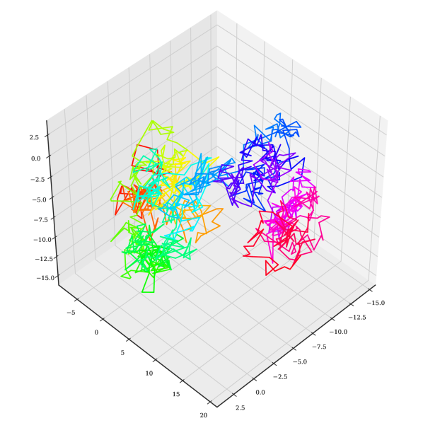
(a) $H=0.3$

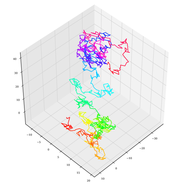
(b) $H=0.5$

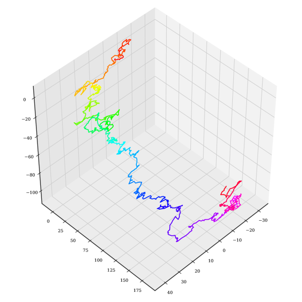
(c) $H=0.7$

Figure 1: Trajectories of fBm in three-dimensional space. The colors indicate the evolution over time. The Hurst parameter $H$ corresponds to the raggedness of the trajectory, with a higher value leading to a smoother motion.

2.2 Fractal Dimension

The notion of dimension is central to our analysis. One that we are most familiar with is the ambient dimension. Roughly speaking, a dimension describes how much space a set occupies near each of its points. For instance, $\mathbb{R}^{d}$ as a vector space has an ambient dimension of $d$ since $d$ different coordinates are required to identify a point in this space. Fractal dimension, however, extends this notion to the fractional case. While it has proven very useful in many mathematical fields such as number theory and dynamical systems, there are many different ways to define fractal dimension, and not all the definitions are equivalent to each other. Of the wide variety of fractal dimensions, we focus on probably the most important box-counting and Hausdorff dimensions.

Box-counting dimension. Suppose $\mathcal{K}$ is a non-empty subset of $\mathbb{R}^{d}$, and the diameter of $\mathcal{K}$ is defined as $\mathrm{diam}(\mathcal{K})=\sup\{\|x-y\|:x,y\in\mathcal{K}\}$. For any non-empty bounded subset $\mathcal{W}$ of $\mathbb{R}^{d}$, let $N_{\delta}(\mathcal{W})$ be the least number of subsets $\{\mathcal{K}_{i}\}$ of diameter at most $\delta$ to cover $\mathcal{W}$, that is, $\mathcal{W}\subseteq\cup_{i=1}^{N_{\delta}(\mathcal{W})}\mathcal{K}_{i}$ and $\mathrm{diam}(\mathcal{K}_{i})\leq\delta$ for each $i$. Then, the lower and upper box-counting dimensions of $\mathcal{W}$, respectively, are defined as

$$\underline{\dim}_{\mathrm{B}}\mathcal{W}=\varliminf_{{\delta\rightarrow 0}}\frac{\log N_{\delta}(\mathcal{W})}{\log(1/\delta)},$$

and

$$\overline{\dim}_{\mathrm{B}}\mathcal{W}=\varlimsup_{{\delta\rightarrow 0}}\frac{\log N_{\delta}(\mathcal{W})}{\log(1/\delta)}.$$

Note that $\underline{\dim}_{\mathrm{B}}\mathcal{W}\leq\overline{\dim}_{\mathrm{B}}\mathcal{{W}}$ and if the equality holds, the box-counting dimension of $\mathcal{W}$ is then denoted by

$$\dim_{\mathrm{B}}\mathcal{W}=\lim_{{\delta\rightarrow 0}}\frac{\log N_{\delta}(\mathcal{W})}{\log(1/\delta)}.$$

The popularity of the box-counting dimension is largely due to its intuitive definition and relative ease of empirical calculation. By contrast, the Hausdorff dimension below is defined in terms of measure theory and is mathematically convenient to work with. Consequently, a disadvantage of the Hausdorff dimension is that it is often difficult to estimate by computational methods. However, for a proper understanding of fractal geometry, familiarity with the Hausdorff dimension is essential.

Hausdorff dimension. Let $\{\mathcal{K}_{i}\}_{i=1}^{\infty}$ be a $\delta$-cover of a non-empty bounded set $\mathcal{W}$, and for each ${\alpha}\geq 0$, we call

$$\mathcal{H}^{\alpha}(\mathcal{W})=\lim_{{\delta\rightarrow 0}}\left\{\sum_{i=1}^{\infty}\mathrm{diam}(\mathcal{K}_{i})^{\alpha}:\mathcal{W}\subseteq\cup_{i=1}^{\infty}\mathcal{K}_{i},\mathrm{diam}(\mathcal{K}_{i})<\delta\right\},$$

the $\alpha$-dimensional Hausdorff measure of $\mathcal{W}$. Usually, it equals $0$ or $\infty$. The critical value of $\alpha$ at which $\mathcal{H}^{\alpha}(\mathcal{W})$ jumps from $\infty$ to $0$ is referred to as the Hausdorff dimension. Rigorously, it is defined as

$$\dim_{\mathrm{H}}\mathcal{W} =\inf\left\{\alpha\geq 0:\mathcal{H}^{\alpha}(\mathcal{W})=0\right\}$$

$$=\sup\left\{\alpha\geq 0:\mathcal{H}^{\alpha}(\mathcal{W})=\infty\right\}.$$

Generically, for the box-counting and Hausdorff dimension, we have the inequality: $\dim_{\mathrm{H}}\mathcal{W}\leq\dim_{\mathrm{B}}\mathcal{W}$. For example, considering the set of rationals in $[0,1]$, the Hausdorff dimension is 0, while the box-counting dimension is 1. Although they are not equivalent to each other, for some fractals, they are sometimes equal (Mattila, 1999, Theorem 5.7).

2.3 Statistical Learning Methodology

Let $\mathcal{X}\subseteq\mathbb{R}^{p}$ be the input space and $\mathcal{Y}\subseteq\mathbb{R}^{q}$ the output or label space, we assume that the pairs $(X,Y)\in\mathcal{X}\times\mathcal{Y}$ are random variables that are distributed according to an unknown distribution $\mathfrak{D}$. After seeing a sequence of $m$ i.i.d. pairs $(X_{i},Y_{i})$ sampled according to $\mathfrak{D}$, the goal of supervised learning is to construct a hypothesis $f:\mathcal{X}\mapsto\mathcal{Y}$ which predicts $Y$ from $X$. In the special case of DNNs, the hypothesis $f\in\mathcal{F}$ is dependent on the corresponding network parameter $W\in\mathbb{R}^{d}$. For convenience, let $Z_{i}=(X_{i},Y_{i})$ and $Z=(X,Y)$. In addition, we denote a training set of size $m$ by $S=(Z_{1},\ldots,Z_{m})$.

To assess the quality of estimated parameter $W$, we consider a non-negative loss function $\ell:\mathbb{R}^{d}\times\mathcal{Z}\to\mathbb{R}_{+}$, such that $\mathcal{\ell}(W;Z)$ quantifies the loss for a particular choice of neural network with parameter $W\in\mathbb{R}^{d}$ with respect to an example $Z\in\mathcal{Z}$. To find out the neural network that attains the lowest loss, we need to minimize the population loss given by

$$R(W)=\underset{Z\sim\mathfrak{D}}{\mathbb{E}}\left[\ell(W;Z)\right].$$

However, due to the unknown data distribution $\mathfrak{D}$, we use the empirical loss over the training set $S$ as a surrogate for the population loss,

$$\widehat{R}_{S}(W)=\frac{1}{m}\sum_{i=1}^{m}\ell(W;Z_{i}).$$

The population loss is also known as the generalization error. The difference between $R(W)$ and $\widehat{R}_{S}(W)$ is referred to as the generalization gap. In the realizable case where the empirical loss equals zero, the generalization gap is interchangeable with the generalization error.

3 Related Literature

In this section, we first survey previous works on generalization and then review the related works where SGD is treated as an SDE analogy.

Generalization. Apart from norm-based bounds, there are still several important classes of generalization bounds. One class is the stability-based bounds, which are built upon the conjecture that if the output of an algorithm is weakly dependent on the training set, then it can be shown to be generalizable (Littlestone and Warmuth, 1986). Especially, the algorithmic stability considers how sensitive the output of an algorithm is when removing one single example from the training set (Bousquet and Elisseeff, 2002; Hardt et al., 2016; Mou et al., 2018). Different from generalization bounds that are based on complexity measures of the hypothesis set used for learning, this approach leads to a finer guarantee by taking into account the properties of a specific algorithm.

Another line of studying generalization relies on the neural tangent kernel (NTK), with which infinite-width DNNs evolve in the function space as linear models (Jacot et al., 2018; Lee et al., 2019). Like the norm-based bounds, the NTK-based bounds also aim to bound the Rademacher complexity of the hypothesis set, which usually depends on the distance of the weights from the initialization (Arora et al., 2019). Similar results are extended to networks with any depth as well (Cao and Gu, 2019). The ease of theoretical analysis of NTK, however, prevents its wide usage on realistic DNNs as assumptions such as infinite width and infinitesimal learning rate are sometimes hard to match in practice.

Thirdly, the correlation between the flatness of the loss landscape and generalization has also attracted numerous attention (Hochreiter and Schmidhuber, 1997; Keskar et al., 2017; Dinh et al., 2017). Empirically, they find that models ending in flat minima, which are indicated by small Hessian eigenvalues, usually generalize well. Based on the flatness of minima found by SGD, a deterministic PAC-Bayes bound is also proposed (Banerjee et al., 2020). However, the flat minima alone do not suffice to explain the generalization behavior of DNNs and should be complemented with some other measures such as the norm of weights (Neyshabur et al., 2018).

Very recently, similar to our study, generalization is also related to the geometric structure of the optimization trajectory (Simsekli et al., 2020). However, the theoretical underpinning of Simsekli et al. (2020) might be flawed under certain conditions (Xie et al., 2021). Unlike Hurst parameter, their proposed upper Blumenthal-Getoor (BG) index fails to capture the correct trend with generalization gap in scenarios such as changing the training set size, as shown in Section 5.

Discrete-time SGD and continuous-time SDE. Before employing SDE to approximate SGD, there are many convergence results for SGD and its variants in the literature (Bach and Moulines, 2011; Needell et al., 2014; Défossez and Bach, 2015). However, most of these analysis techniques are ad hoc and lack a systematic approach to studying the behavior of SGD dynamics. To address this issue, Li et al. (2015) generalize the method of modified equations (Noh and Protter, 1963; Hirt, 1968; Warming and Hyett, 1974) to the stochastic setting, where discrete-time stochastic gradient algorithms are approximated by continuous-time SDEs with a noising term.

One central ingredient for SDE approximation is SGN incurred by SGD during the training process. In the simplest case, SGN is assumed to follow an isotropic Gaussian, from which the equilibrium of SDE is given by the Gibbs distribution (Jastrzebski et al., 2017). By considering the covariance structure, Zhu et al. (2019) show that anisotropic gradient noise is superior to isotropic gradient noise in terms of the escaping efficiency from local minima. Presuming that the covariance of SGN may be parameter-dependent, Smith et al. (2020) successfully explain the phenomenon of sudden rising error after decaying the learning rate and derive a linear scaling rule for infinitesimal learning rate. Moreover, under the assumption that the covariance is constant in the vicinity of local minima, Mandt et al. (2017) demonstrate how SGD could be modified to perform approximate Bayesian posterior sampling. The assumption that SGN follows a Gaussian distribution is first challenged by Simsekli et al. (2019) and Nguyen et al. (2019) and they propose that SGN is heavy-tailed and follows $\alpha$-stable Lévy motion instead. However, a recent work (Xie et al., 2021) argues that the method of Simsekli et al. (2019) to estimate SGN is flawed and SGN might still be Gaussian.

Despite the popularity of employing SDEs to study SGD, theoretical justification for this approximation, in general, is validated only for small learning rates (Hu et al., 2017; Yaida, 2019; Li et al., 2019). Recently, Li et al. (2021) propose an efficient simulation algorithm SVAG that provably converges to the vanilla Itô SDE approximation and recover a theoretically provable and empirically testable necessary condition for the SDE approximation to hold.

4 Bounding the Maximal Generalization Gap

In this section, we first formally state the problem to be solved and then present the main results in two steps: (1) bounding the maximal generalization gap in terms of the Rademacher complexity by invoking the hypothesis set stability (see Section 4.2); (2) relating the Rademacher complexity of the optimization trajectory to its Hausdorff dimension using existing covering number techniques (see Section 4.3).

4.1 Problem Setup

Given a training set $S=(Z_{1},\ldots,Z_{m})$ and a loss function $\ell:\mathbb{R}^{d}\times\mathcal{Z}\mapsto\mathbb{R}_{+}$, the $k$th update of SGD is described as

$$W_{k+1}=W_{k}-\eta\nabla\hat{\ell}_{k}(W_{k}),$$ (1)

where $\eta$ is the learning rate and $\nabla\hat{\ell}_{k}(W_{k})$ is an unbiased stochastic gradient, which is computed by

$$\nabla\hat{\ell}_{k}(W_{k})=\frac{1}{|I_{k}|}\sum_{i\in I_{k}}\nabla\ell(W_{k};Z_{i}),$$

where $I_{k}$ is the set of example indices that are i.i.d. drawn from $[m]=\{1,\ldots,m\}$ and $|\cdot|$ is used to denote cardinality. Many studies have shown that mini-batch stochastic gradient $\nabla\hat{\ell}_{k}(W_{k})$ outperforms the full-batch gradient $\nabla\ell_{k}(W_{k})$ in terms of speed and accuracy (Zhu et al., 2019). The difference between the mini-batch stochastic gradient $\nabla\hat{\ell}_{k}(W_{k})$ and its full-batch counterpart $\nabla\ell_{k}(W_{k})$ is the so-called SGN, defined as

$$\lambda_{k}=\nabla\hat{\ell}_{k}(W_{k})-\nabla\ell_{k}(W_{k}).$$

If one assumes that $\eta$ is small enough and $\lambda_{k}$ follows a zero-mean distribution, the SGD recursion can be seen as a first-order discretization of a continuous-time SDE.

Recently, perspectives from SDEs have provided many insights on studying the generalization behavior of DNNs through the asymptotic convergence rate and local dynamic behavior of SGD (Mandt et al., 2017; Simsekli et al., 2019; Xie et al., 2021). In our analysis, we will in particular consider the case where SGD is viewed as the Euler-Maruyama discretization of the following SDE (Tan et al., 2021),

$$\mathrm{d}W_{t}=-\mu(W_{t},t)\mathrm{d}t+\sigma(W_{t},t)\mathrm{d}B_{t}^{H},$$ (2)

where $\mu(W_{t},t)$ is the drift coefficient, $\sigma(W_{t},t)$ is the diffusion coefficient, and $B_{t}^{H}$ represents fBm with Hurst parameter $H$. Such class of SDEs admits SGN produced at different iterations to be mutually interdependent, which significantly varies from previous studies where SGN is assumed to follow a Gaussian distribution (Li et al., 2017; Mandt et al., 2017; Li et al., 2019).

A pairwise correspondence between discrete-time SGD recursion (1) and continuous-time SDE driven by fBm (2) can be easily established. For a finite number of iterations $K$ of the optimization process, let $\mathcal{W}_{1:K}=\left\{W_{1},\ldots,W_{k},\ldots,W_{K}\right\}$ be the entire evolution of network parameter, where $W_{k}\in\mathbb{R}^{d}$ is the network parameter picked by SGD at $k$th iteration. When the learning rate $\eta$ is small enough, for a given $t\in[k\eta,(k+1)\eta)$, we can always define a stochastic process $\widehat{W}_{t}$ as the interpolation of two successive iterates $W_{k}$ and $W_{k+1}$ such that $\widehat{W}_{k\eta}=W_{k}$ for all $k$. This approach is frequently adopted in SDE literature (Mishura and Shevchenko, 2008) and allows the trajectory to be continuous to represent the SGD recursion.

In contrast to the discrete-time trajectory $\mathcal{W}_{1:K}$, for any training set $S\in\mathcal{Z}^{m}$, let $\mathcal{W}_{S}$ denote the collection of network parameters in the continuous-time trajectory over a period of time $t\in[0,T]$,

$$\mathcal{W}_{S}=\left\{W\in\mathbb{R}^{d}:\exists~{}t\in[0,T],W=\widehat{W}_{t}\right\},$$

and $\mathcal{W}=\cup_{S\in\mathcal{Z}^{m}}\mathcal{W}_{S}$ the union of all possible network parameters that SGD explores. Moreover, let $\mathcal{G}_{S}$ denote the loss functions associated to $\mathcal{W}_{S}$ mapping from $\mathcal{Z}=\mathcal{X}\times\mathcal{Y}$ to $\mathbb{R}_{+}$,

$$\mathcal{G}_{S}=\{Z\mapsto\ell(W;Z):W\in\mathcal{W}_{S}\},$$

and let $\mathcal{G}=\cup_{S\in\mathcal{Z}^{m}}\mathcal{G}_{S}$ denote the union of loss functions $\mathcal{G}_{S}$.

For any $\epsilon>0$, our goal is to bound the following term

$$\mathbb{P}\left[\sup_{W\in\mathcal{W}_{S}}|\widehat{R}_{S}(W)-R(W)|\geq\epsilon\right],$$

which is trajectory-dependent and differs from what is usually studied where $\mathcal{W}_{S}$ is replaced by a pre-specified hypothesis set. It should be noted that we do not consider bounding the maximal generalization gap over the discrete-time trajectory since dealing with the continuous-time situation is mathematically more convenient. In addition, the maximal generalization gap over the discrete-time trajectory $\mathcal{W}_{1:K}$ is controlled by that over the continuous-time trajectory $\mathcal{W}_{S}$. In the sequel, we will present our first result in terms of the Rademacher complexity $\mathfrak{R}_{m}(\mathcal{G})$ (Bartlett and Mendelson, 2002), which is defined as

$$\mathfrak{R}_{m}(\mathcal{G})\triangleq\frac{1}{m}~{}\underset{\boldsymbol{\sigma}\sim\{\pm 1\}^{m}}{\mathbb{E}}\left[\sup_{W\in\mathcal{W}}\sum_{i=1}^{m}\sigma_{i}~{}\ell(W;Z_{i})\right],$$

where the Rademacher variables $\sigma_{i}$ are i.i.d. with $\mathbb{P}(\sigma_{i}=\pm 1)=1/2$.

4.2 Hypothesis Set Stability and Generalization

Algorithmic stability (Bousquet and Elisseeff, 2002) describes how a learning algorithm is perturbed by small changes to its input. In this section, we will use a more broad concept of stability, hypothesis set stability (Foster et al., 2019), which admits the algorithmic stability as a special case.

Definition 2 (Hypothesis Set Stability)

Let $\mathcal{W}={\cup}_{S\in\mathcal{Z}^{m}}\mathcal{W}_{S}$ be the collection of data-dependent network parameters. We say $\mathcal{W}$ is $\beta$-stable if for some $\beta\geq 0$ and for any two samples $S$ and $S^{\prime}$ of size $m$ differing only by an example, the following holds:

$$\forall~{}W\in\mathcal{W}_{S},~{}\exists~{}W^{\prime}\in\mathcal{W}_{S^{\prime}}:~{}\forall~{}Z\in\mathcal{Z},~{}|\ell(W;Z)-\ell(W^{\prime};Z)|\leq\beta.$$

Under this assumption, two training sets differing only one single point will cause the learning algorithm to return two sets of network parameters that are very close. Namely, any network parameter appearing in one set admits a counterpart in another set with at most a $\beta$-similar loss. To derive the maximal generalization gap in terms of $\mathfrak{R}(\mathcal{G})$, we need to use an inequality that relates moments of multi-dimensional random functions to their first-order finite differences. This inequality is attributed to McDiarmid et al. (1989) and gives an exponential bound.

Theorem 3 (McDiarmid Inequality)

Assume that $S$ is an i.i.d. sample of size $m$ drawn from $\mathfrak{D}$ and $S^{i}$ differs from $S$ exactly by an example $Z_{i}^{\prime}$, which is also drawn from $\mathfrak{D}$ and is independent of $S$. Let $\Phi:\mathcal{Z}^{m}\mapsto\mathbb{R}$ be any measurable function for which there exists constants $o_{i}~{}(i=1,\ldots,m)$ such that

$$\sup_{S\in\mathcal{Z}^{m},Z_{i}^{\prime}\in\mathcal{Z}}\left|\Phi(S)-\Phi\left(S^{i}\right)\right|\leq o_{i},$$

then

$$\mathbb{P}\left[\Phi(S)-\mathbb{E}_{S}[\Phi(S)]\geq\epsilon\right]\leq e^{-2\epsilon^{2}/\sum_{i=1}^{m}o_{i}^{2}}.$$

On the basis of the McDiarmid inequality, we now prove that the maximal generalization gap is controlled by the Rademacher complexity of the hypothesis set that SGD explores.

Theorem 4

Assume that the loss function $\ell:\mathbb{R}^{d}\times\mathcal{Z}\mapsto\mathbb{R}_{+}$ is bounded in $[0,\zeta]$ and $\mathcal{W}=\cup_{S\in\mathcal{Z}^{m}}\mathcal{W}_{S}$ is $\beta$-stable. Then, for any $\tau>0$, with probability at least $1-\tau$ over the draw of an i.i.d. sample $S\in\mathcal{Z}^{m}$, the following inequality holds:

$$\forall~{}W\in\mathcal{W}_{S},R(W)\leq\widehat{R}_{S}(W)+2\mathfrak{R}_{m}(\mathcal{G})+(\zeta+2m\beta)\sqrt{\frac{1}{2m}\log{\frac{1}{\tau}}}.$$

Proof  The proof is based on Mohri et al. (2018, Theorem 3.3) and Foster et al. (2019, Theorem 2). For any two samples $S=(Z_{1},\ldots,Z_{m})$ and $S^{\prime}$ which differs from $S$ exactly by an example, say $Z_{m}$ in $S$ and $Z_{m}^{\prime}$ in $S^{\prime}$, we define the function $\Phi(S,S^{\prime})$ as follows

$$\Phi(S,S^{\prime})=\sup_{W\in\mathcal{W}_{S}}\left[\mathcal{R}(W)-\widehat{\mathcal{R}}_{S^{\prime}}(W)\right].$$

It is obvious that $\mathbb{E}_{S\sim\mathfrak{D}^{m}}[\Phi(S,S)]=\mathbb{E}_{S^{\prime}\sim\mathfrak{D}^{m}}[\Phi(S^{\prime},S^{\prime})]$, so we are able to leverage McDiarmid’s inequality directly. Consider the following decomposition

$$\Phi(S,S)-\Phi(S^{\prime},S^{\prime})=\left[\Phi(S,S)-\Phi(S,S^{\prime})\right]+\left[\Phi(S,S^{\prime})-\Phi(S^{\prime},S^{\prime})\right].$$ (3)

By the sud-addtivity of the supremum function, the first term of Equation (3) can be upper-bounded as follows

$$\Phi(S,S)-\Phi(S,S^{\prime}) =\sup_{W\in\mathcal{W}_{S}}[\mathcal{R}(W)-\widehat{\mathcal{R}}_{S}(W)]-\sup_{W\in\mathcal{W}_{S}}[\mathcal{R}(W)-\widehat{\mathcal{R}}_{S^{\prime}}(W)]$$

$$\leq\sup_{W\in\mathcal{W}_{S}}\left[\widehat{\mathcal{R}}_{S^{\prime}}(W)-\widehat{\mathcal{R}}_{S}(W)\right]$$

$$=\sup_{W\in\mathcal{W}_{S}}\frac{1}{m}[\ell(W;Z_{m}^{\prime})-\ell(W;Z_{m})]$$

$$\leq\frac{\zeta}{m}.$$ (4)

The last inequality holds since the loss function $\ell$ is bounded and non-negative. As to the second part of Equation (3), we have

$$\Phi(S,S^{\prime})-\Phi(S^{\prime},S^{\prime})=\sup_{W\in\mathcal{W}_{S}}\left[\mathcal{R}(W)-\widehat{\mathcal{R}}_{S^{\prime}}(W)\right]-\sup_{W\in\mathcal{W}_{S^{\prime}}}\left[\mathcal{R}(W)-\widehat{\mathcal{R}}_{S^{\prime}}(W)\right].$$

For any $\epsilon>0$, on one hand, following the definition of the supremum function, there exists some $W^{\ast}\in\mathcal{W}_{S}$ such that

$$\sup_{W\in\mathcal{W}_{S}}\left[\mathcal{R}(W)-\widehat{\mathcal{R}}_{S^{\prime}}(W)\right]\leq\left[\mathcal{R}(W^{\ast})-\widehat{\mathcal{R}}_{S^{\prime}}(W^{\ast})\right]+\epsilon.$$

Meanwhile, since $\cup_{S\in\mathcal{Z}^{m}}\mathcal{W}_{S}$ is $\beta$-stable, there exists some $W^{\prime}\in\mathcal{W}_{S^{\prime}}$ such that for all $Z\in\mathcal{Z}$, $|\ell(W^{\ast};Z)-\ell(W^{\prime};Z)|\leq\beta$. Hence, we have

$$\Phi(S,S^{\prime})-\Phi(S^{\prime},S^{\prime}) \leq\left[\mathcal{R}(W^{\ast})-\widehat{\mathcal{R}}_{S^{\prime}}(W^{\ast})\right]+\epsilon-\sup_{W\in\mathcal{W}_{S^{\prime}}}\left[\mathcal{R}(W)-\widehat{\mathcal{R}}_{S^{\prime}}(W)\right]$$

$$\leq\left[\mathcal{R}(W^{\ast})-\widehat{\mathcal{R}}_{S^{\prime}}(W^{\ast})\right]+\epsilon-\left[\mathcal{R}(W^{\prime})-\widehat{\mathcal{R}}_{S^{\prime}}(W^{\prime})\right]$$

$$=\epsilon+\left[\mathcal{R}(W^{\ast})-\mathcal{R}(W^{\prime})\right]+\left[\widehat{\mathcal{R}}_{S^{\prime}}(W^{\prime})-\widehat{\mathcal{R}}_{S^{\prime}}(W^{\ast})\right]$$

$$=\epsilon+\underset{Z\sim\mathfrak{D}}{\mathbb{E}}\left[\ell(W^{\ast};Z)-\ell(W^{\prime};Z)\right]+\left[\widehat{\mathcal{R}}_{S^{\prime}}(W^{\prime})-\widehat{\mathcal{R}}_{S^{\prime}}(W^{\ast})\right]$$

$$\leq\epsilon+\beta+\left[\widehat{\mathcal{R}}_{S^{\prime}}(W^{\prime})-\widehat{\mathcal{R}}_{S^{\prime}}(W^{\ast})\right]$$

$$=\epsilon+\beta+\frac{1}{m}\sum_{Z_{i}\in S^{\prime}}\left[\ell(W^{\prime};Z_{i})-\ell(W^{\ast};Z_{i})\right]$$

$$\leq\epsilon+2\beta.$$

Since the above inequality holds for any $\epsilon>0$, it implies that

$$\Phi(S,S^{\prime})-\Phi(S^{\prime},S^{\prime})\leq 2\beta.$$ (5)

Therefore, by summing up Equations (4) and (5), we have

$$\Phi(S,S)-\Phi(S^{\prime},S^{\prime})\leq\frac{\zeta}{m}+2\beta.$$

Finally, by invoking McDiarmid inequality, for any $\tau>0$, with probability at least $1-\tau$, we have

$$\Phi(S,S)\leq\mathbb{E}[\Phi(S,S)]+(\zeta+2m\beta)\sqrt{\frac{1}{2m}\log{\frac{1}{\tau}}}.$$ (6)

In the last step, we will prove that $\mathbb{E}[\Phi(S,S)]$ is bounded by $2\mathfrak{R}_{m}(\mathcal{G})$:

$$\underset{{S\sim\mathfrak{D}^{m}}}{\mathbb{E}}[\Phi(S,S)] =\underset{S\sim\mathfrak{D}^{m}}{\mathbb{E}}\left[\sup_{W\in\mathcal{W}_{S}}\left[\mathcal{R}(W)-\widehat{\mathcal{R}}_{S}(W)\right]\right]$$

$$=\underset{S\sim\mathfrak{D}^{m}}{\mathbb{E}}\left[\sup_{W\in\mathcal{W}_{S}}\underset{Q\sim\mathfrak{D}^{m}}{\mathbb{E}}\left[\widehat{\mathcal{R}}_{Q}(W)-\widehat{\mathcal{R}}_{S}(W)\right]\right]$$ (7)

$$\leq\underset{S,Q\sim\mathfrak{D}^{m}}{\mathbb{E}}\sup_{W\in\mathcal{W}_{S}}\left[\widehat{\mathcal{R}}_{Q}(W)-\widehat{\mathcal{R}}_{S}(W)\right]$$ (8)

$$=\underset{S,Q\sim\mathfrak{D}^{m}}{\mathbb{E}}\sup_{W\in\mathcal{W}_{S}}\frac{1}{m}\sum_{i=1}^{m}\left[\ell(W;Z_{i}^{Q})-\ell(W;Z_{i}^{S})\right]$$

$$\leq\underset{S,Q\sim\mathfrak{D}^{m}}{\mathbb{E}}\sup_{W\in\mathcal{W}}\frac{1}{m}\sum_{i=1}^{m}\left[\ell(W;Z_{i}^{Q})-\ell(W;Z_{i}^{S})\right]$$ (9)

$$=\underset{S,Q\sim\mathfrak{D}^{m}}{\mathbb{E}}\left[\underset{\boldsymbol{\sigma}\sim\{\pm 1\}^{m}}{\mathbb{E}}\left[\sup_{W\in\mathcal{W}}\frac{1}{m}\sum_{i=1}^{m}\sigma_{i}\left[\ell(W;Z_{i}^{Q})-\ell(W;Z_{i}^{S})\right]\right]\right]$$ (10)

$$\leq\underset{\stackrel{{\scriptstyle S,Q\sim\mathfrak{D}^{m}}}{{\boldsymbol{\sigma}\sim\{\pm 1\}^{m}}}}{\mathbb{E}}\left[\sup_{W\in\mathcal{W}}\frac{1}{m}\sum_{i=1}^{m}\sigma_{i}\ell(W;Z_{i}^{Q})+\sup_{W\in\mathcal{W}}\frac{1}{m}\sum_{i=1}^{m}-\sigma_{i}\ell(W;Z_{i}^{S})\right]$$ (11)

$$=\underset{\stackrel{{\scriptstyle S,Q\sim\mathfrak{D}^{m}}}{{\boldsymbol{\sigma}\sim\{\pm 1\}^{m}}}}{\mathbb{E}}\left[\sup_{W\in\mathcal{W}}\frac{1}{m}\sum_{i=1}^{m}\sigma_{i}\ell(W;Z_{i}^{Q})+\sup_{W\in\mathcal{W}}\frac{1}{m}\sum_{i=1}^{m}\sigma_{i}\ell(W;Z_{i}^{S})\right]$$ (12)

$$=2\mathfrak{R}_{m}(\mathcal{G}).$$

Equation (7) uses the fact that the points in $Q$ are i.i.d. drawn from $\mathfrak{D}$ and thus $\underset{Q\sim\mathfrak{D}^{m}}{\mathbb{E}}\widehat{\mathcal{R}}_{Q}(W)=\mathcal{R}(W)$. Inequality (8) holds due to the fact that the supremum of expectation is smaller than the expectation of the supremum. Besides, we introduce a superscript to represent $Z_{i}^{Q}\in Q$ and $Z_{i}^{S}\in S$. Inequality (9) stems from the fact that $\mathcal{W}_{S}\subseteq\mathcal{W}$ and Equation (10) holds since $\mathcal{W}$ is independent of $S$ and $Q$ and introducing Rademacher variables $\mathbf{\sigma}$ does not affect the overall expectation. Equation (11) is valid due to the sub-addtivity of the supremum function. Finally, Equation (12) holds since the variables $\sigma_{i}$ and $-\sigma_{i}$ are distributed in the same way.

Combining this result with Equation (6) completes the proof.  

Remark 5

This result is similar to the generalization bound derived from the Rademacher complexity for a fixed hypothesis set (Mohri et al., 2018, Theorem 3.3), except for the extra coefficient $\beta$. When $\beta=0$, it implies that $\mathcal{W}_{S}$ remains the same for all $S\in\mathcal{Z}^{m}$ and the result degenerates to the special case of Mohri et al. (2018, Theorem 3.3). There indeed exists a positive correlation between $\beta$ and $\mathfrak{R}(\mathcal{G})$. This can be illustrated by the fact that Rademacher complexity characterizes the richness of a function class. When $\beta$ is small, similar training sets result in loss vectors pointing in almost the same direction, then the Rademacher complexity is low due to the expectation over the random Rademacher variable. By contrast, when $\beta$ is large, similar training sets result in loss vectors in many different directions and thus the Rademacher complexity stays high.

Though we have derived an upper bound over the maximal generalization gap, we wish to determine $\mathfrak{R}(\mathcal{G})$ by taking into account the Hausdorff dimension of the optimization trajectory. The Hausdorff dimension determines the raggedness of the optimization trajectory and characterizes the dynamic behavior of SGD around the local minimum.

4.3 Rademacher Complexity of the Optimization Trajectory

Let $\mathcal{G}\circ S$ be the set of all possible loss evaluations that a loss function $g\in\mathcal{G}$ can achieve over the training set $S$, namely,

$$\mathcal{G}\circ S=\left\{\left(g(Z_{1}),\ldots,g(Z_{m})\right):g\in\mathcal{G}\right\}.$$

To simplify the notation, let $\mathcal{H}=\mathcal{G}\circ S$. According to the definition of Rademacher complexity, $\mathfrak{R}(\mathcal{G})$ is actually the same as $\mathfrak{R}(\mathcal{H})$. We will first present several assumptions used in our theoretical analysis. Thereafter, the assumptions are explained explicitly and the bound over $\mathfrak{R}(\mathcal{H})$ is stated.

Assumption 6

The loss function $\ell:\mathbb{R}^{d}\times\mathcal{Z}\mapsto\mathbb{R}_{+}$ is Lipschitz continuous with respect to its first argument.

If a mapping satisfies the Lipschitz continuity, then the Hausdorff dimension of the image is no greater than the Hausdorff dimension of the preimage (Falconer, 2004, Proposition 3.3). Consequently, we arrive at the conclusion that $\dim_{\mathrm{H}}\mathcal{H}\leq\dim_{\mathrm{H}}\mathcal{W}$. This inequality is critical in our analysis and allows us to bound the loss space with the Hausdorff dimension of the optimization trajectory.

Assumption 7

The drift coefficient $\mu(W_{t},t)$ and diffusion coefficient $\sigma(W_{t},t)$ in Equation (2) are both bounded vector fields on $\mathbb{R}^{d}$.

This assumption is reasonable due to the existence of batch normalization (Ioffe and Szegedy, 2015), weight decay (Krogh and Hertz, 1992) and other popular tricks. Under this assumption, the Hausdorff dimension of the optimization trajectory implemented by Equation (2) attains a value of $1/H$ as a consequence of $d\gg 1/H$, where $d$ represents the number of network parameters (Lou and Ouyang, 2016).

Assumption 8

The data distribution $\mathfrak{D}$ is countable.

We note that this assumption is crucial to our results. Thanks to this condition, we are able to invoke the countable stability of the Hausdorff dimension to determine the upper bound of $\dim_{\mathrm{H}}\mathcal{W}$ in terms of the Hurst parameter $H$.

Assumption 9

Given the data distribution $\mathfrak{D}$, for any i.i.d. sample of fixed size, the Hurst parameter $H$ is determined only by the network architecture and the optimizer hyperparameters such as the learning rate and mini-batch size.

By imposing this condition, we argue that the Hurst parameter $H$ behaves like an order parameter in a physical system. That is, the Hurst parameter $H$ remains unchanged when the neural network receives different training examples from the same data distribution.

Assumption 10

Let $\mathcal{H}$ be a non-empty bounded subset of $\mathbb{R}_{+}^{m}$ and there exists a Borel measure $\nu$ on $\mathbb{R}_{+}^{m}$ and positive numbers $a$, $b$, $r_{0}$ and $\kappa$ such that $0<\nu(\mathcal{H})\leq\nu(\mathbb{R}_{+}^{m})<\infty$ and for $h\in\mathcal{H}$

$$0<ar^{\kappa}\leq\nu(B_{\mathrm{distance}}(h,r))\leq br^{\kappa}<\infty,\quad 0<r<r_{0},$$

where

$$B_{\mathrm{distance}}(h,r)=\{h^{\prime}\in\mathcal{H}|distance(h,h^{\prime})<r\}.$$

This condition indeed implies that $\dim_{\mathrm{B}}\mathcal{H}=\dim_{\mathrm{H}}\mathcal{H}=\kappa$, and is commonly used in fractal geometry to ensure the trajectory is regular enough so that the Hausdorff dimension is equivalent to the box-counting dimension and so we can use the covering number techniques (Mattila, 1999, Theorem 5.7).

Based on these assumptions, we are ready to present an upper bound over $\mathfrak{R}(\mathcal{H})$. To the best of our knowledge, we are the first to bound the Rademacher complexity of the trajectory-dependent hypothesis set.

Theorem 11

Let $\mathcal{H}$ be defined as above and denote its diameter by $\mathrm{diam}(\mathcal{H})=\sup\{\|h-h^{\prime}\|:h,h^{\prime}\in\mathcal{H}\}$. Assume the assumptions (6)-(10) hold, then

$$\mathfrak{R}(\mathcal{H})\leq\frac{12\mathrm{diam}(\mathcal{H})}{m}\sqrt{\frac{\log 4}{H}}.$$ (13)

Proof  As $\mathcal{H}$ lives in a very high-dimensional subspace of $\mathbb{R}^{m}$, $\mathrm{diam}(\mathcal{H})$ actually is very large and scales with $\mathcal{O}(\sqrt{m})$ in practice. Without loss of generality, we assume that $\mathrm{diam}(\mathcal{H})\geq 1$. Let $\{\delta_{k}\}$ be a monotonically decreasing sequence such that $\delta_{k}=\mathrm{diam}(\mathcal{H})2^{-k}$ for all $k\in\mathbb{Z}$. According to the definition of the box-counting dimension, we have the following equation

$$\dim_{\mathrm{B}}\mathcal{H}=\lim_{{\delta\rightarrow 0}}\frac{\log N_{\delta}(\mathcal{H})}{-\log\delta}.$$

On one hand, for any $\epsilon>0$, there exists a $k_{\epsilon}$ such that for all $k>k_{\epsilon}$,

$$\log N_{\delta_{k}}(\mathcal{H})\leq(\dim_{\mathrm{B}}\mathcal{H}+\epsilon)\log(\delta_{k}^{-1}).$$

In particular, we choose $\epsilon=\dim_{\mathrm{B}}\mathcal{H}$, and we have for all $k>k_{\epsilon}$,

$$\log N_{\delta_{k}}(\mathcal{H})\leq k\log 4\dim_{\mathrm{B}}\mathcal{H}\leq k^{2}\log 4\dim_{\mathrm{B}}\mathcal{H}.$$ (14)

On the other hand, by selecting $k_{i}=\operatorname*{arg\,inf}\limits_{k\geq i}{\frac{\log N_{\delta_{k}}(\mathcal{H})}{-\log\delta_{k}}}$, we can construct a monotonically increasing sub-sequence {$\frac{\log N_{\delta_{k_{i}}}(\mathcal{H})}{-\log\delta_{k_{i}}}$}, which is also convergent to $\dim_{\mathrm{B}}\mathcal{H}$. Letting $i_{\epsilon}=\operatorname*{arg\,inf}\limits_{i}\{k_{i}\geq k_{\epsilon}\}$, then inequality (14) naturally holds for all $k\geq k_{i_{\epsilon}}$. In the next, we show that inequality (14) applies to $k\leq k_{i_{\epsilon}}$ as well. We will first prove this result for the discrete endpoints $\{k_{i}:i\leq i_{\epsilon}\}$ and then argue this holds for any integers $k\in\left(k_{i},k_{i+1}\right)$. To examine the former case, given $k_{i}<k_{i+1}\leq k_{i_{\epsilon}}$, we have

$${\log N_{\delta_{k_{i}}}(\mathcal{H})}\leq\frac{-\log\delta_{k_{i}}}{-\log\delta_{k_{i+1}}}\log N_{\delta_{k_{i+1}}}(\mathcal{H})\leq\frac{-\log\delta_{k_{i}}}{-\log\delta_{k_{i_{\epsilon}}}}\log N_{\delta_{k_{i_{\epsilon}}}}(\mathcal{H}),$$

implying that

$$\log N_{\delta_{k_{i}}}(\mathcal{H})\leq k_{i}\log 4\dim_{\mathrm{B}}\mathcal{H}\leq k_{i}^{2}\log 4\dim_{\mathrm{B}}\mathcal{H}.$$

To determine the bound for $\log N_{\delta_{k}}(\mathcal{H})$ when $k_{i}<k<k_{i+1}$, two cases need to be separately considered:

(1) If $k_{i+1}\leq k_{i}^{2}$, then we can infer that

$$\log N_{\delta_{k}}(\mathcal{H}) \leq\log N_{\delta_{k_{i+1}}}(\mathcal{H})\leq k_{i+1}\log 4\dim_{\mathrm{B}}\mathcal{H}$$

$$\leq k_{i}^{2}\log 4\dim_{\mathrm{B}}\mathcal{H}\leq k^{2}\log 4\dim_{\mathrm{B}}\mathcal{H};$$

(2) When $k_{i+1}>k_{i}^{2}$, it becomes more tricky. We exclude the $k_{i+1}$ entry from the sequence and reconstruct another monotonically increasing sub-sequence while keeping all the entries before $k_{i+1}$ fixed. It is easy to verify that the new index $\hat{k}_{i+1}$ will not be greater than $k_{i+1}$. Repeat this process until $\hat{k}_{i+1}\leq k_{i}^{2}$, and then we can apply the above result.

Overall, the following inequality holds for all $k\geq 0$

$$\sqrt{\log N_{\delta_{k}}(\mathcal{H})}\leq\sqrt{k^{2}\log 4\dim_{\mathrm{B}}\mathcal{H}}=\sqrt{\log 4\dim_{\mathrm{B}}\mathcal{H}}k.$$ (15)

Recall Dudley’s lemma (Shalev-Shwartz and Ben-David, 2014, Lemma 27.5), we have

$$\mathfrak{R}(\mathcal{H})\leq\frac{12\mathrm{diam}(\mathcal{H})}{m}\sqrt{\dim_{\mathrm{B}}\mathcal{H}\log 4}.$$ (16)

Therefore, the next crucial step is to determine $\dim_{\mathrm{B}}\mathcal{H}$. According to Assumption 10, the box-counting dimension of $\mathcal{H}$ is equivalent to its Hausdorff dimension $\dim_{\mathrm{H}}\mathcal{H}$. Moreover, the loss function is assumed to be Lipschitz continuous, thus we have $\dim_{\mathrm{H}}\mathcal{H}\leq\dim_{\mathrm{H}}\mathcal{W}$ and the inequality now becomes $\dim_{\mathrm{B}}\mathcal{H}\leq\dim_{\mathrm{H}}\mathcal{W}$. Since $\mathfrak{D}$ is countable, then $\mathfrak{D}^{m}$ is countable as well. By invoking the countable stability of the Hausdorff dimension, we have

$$\dim_{\mathrm{H}}\mathcal{W}=\dim_{\mathrm{H}}\cup_{S\in\mathcal{Z}^{m}}\mathcal{W}_{S}=\sup_{S\in\mathcal{Z}^{m}}\dim_{\mathrm{H}}\mathcal{W}_{S}.$$

Meanwhile, for all $S\in\mathcal{Z}^{m}$, $\dim_{\mathrm{H}}\mathcal{W}_{S}$ is bounded by $1/H$ due to Assumption 7. Consequently, we obtain $\dim_{\mathrm{H}}\mathcal{W}\leq 1/H$. Substituting these results into Equation (16) completes the proof.  

Remark 12

The optimization trajectory we discuss here refers to the continuous-time trajectory implemented by SDE (2) rather than the discrete-time trajectory picked by SGD recursion (1) since the Hausdorff dimension of a finite set equals zero and leaves the discussion meaningless. Besides, as the continuous-time trajectory is the interpolation of the discrete-time trajectory, it is easy to conclude that the maximal generalization gap over the discrete-time trajectory is upper bounded by the one over the continuous-time trajectory. This theorem indicates that a larger Hurst parameter of $H$ leads to a smaller Rademacher complexity of the optimization trajectory. This follows from the fact that a large Hurst parameter indicates that the network parameters are persistent with the past and the loss evaluations will largely keep the same direction. As a consequence, the Rademacher complexity as an expectation over the Rademacher variable will be relatively smaller when compared to the case of a smaller Hurst parameter.

4.4 Main Result

Our main result is immediate from Theorem 4 and Theorem 11.

Theorem 13

Assume that $\mathcal{W}=\cup_{S\in\mathcal{Z}^{m}}\mathcal{W}_{S}$ is $\beta$-stable and $\mathrm{diam}(\mathcal{H})$ is defined as above. Assume that the loss function $\ell:\mathbb{R}^{d}\times\mathcal{Z}\mapsto\mathbb{R}_{+}$ is bounded in $[0,\zeta]$ and that the assumptions (6)-(10) hold. Then, with probability of at least $1-\tau$ over i.i.d. sample $S$ of size $m$, the following holds:

$$\forall~{}W\in\mathcal{W}_{S},R(W)\leq\widehat{R}_{S}(W)+\frac{24\zeta\mathrm{diam}(\mathcal{H})}{m}\sqrt{\frac{\log 4}{H}}+(\zeta+2\beta m)\sqrt{\frac{1}{2m}\log{\frac{1}{\tau}}}.$$

This theorem shows that the maximal generalization gap can be controlled by the Hurst parameter $H$ along with other constants inherited from the imposed conditions. Though $H\in(0,1)$ seems too narrow at first glance, we argue that the value of $\mathrm{diam}(\mathcal{H})$ empirically changes in the opposite direction with $H$. A large Hurst parameter of $H$ encourages the optimizer to select a smooth trajectory and end in flat regions where the test errors are low. This finding is central to our work and reminiscent of the phenomenon that flat minima tend to generalize better (Hochreiter and Schmidhuber, 1997; Keskar et al., 2017). The link between the flatness and Hurst parameter can be elaborated as follows. When the curvature is large, it is difficult for the optimizer to escape from the local minima. Accordingly, the resultant trajectory would be ragged and correspond to a large value of $H$. As such, in scenarios such as model selection, we no longer need to calculate the theoretical generalization bound, but rather use a proxy indicator $H$ to assess which model is superior. Though our theoretical analysis is limited to vanilla SGD, empirical results demonstrate that our results also hold for SGD with momentum and weight decay (see Section 5.4).

5 Experiments

In this section, we aim to examine how well the proposed bound predicts the generalization bound over the most common experimental interventions. As a starting point, we first investigate how the bound changes with the training set size. We then study its dependence on the depth (number of layers) and the width (number of channels) of the neural network. The effects of different choices of training hyperparameters such as mini-batch size and learning rate are also discussed. Though our bound is derived from vanilla SGD, the effects of momentum and weight decay are studied as well. Finally, we compare the Hurst parameter against existing generalization indicators, namely the power-law index (Mahoney and Martin, 2019) and the upper Blumenthal-Getoor index (Simsekli et al., 2020).

Implementation details. In this study, we consider three different data sets: CIFAR10 (Krizhevsky et al., 2009), CIFAR100 (Krizhevsky et al., 2009), and SVHN (Netzer et al., 2011). Both CIFAR10 and CIFAR100 are randomly split into training and testing subsets with sizes $5\text{\times}{10}^{4}$ and $1\text{\times}{10}^{4}$, respectively. SVHN is randomly split into a training subset of size $7\text{\times}{10}^{4}$ and a testing subset of size $3\text{\times}{10}^{4}$. We do not use data augmentation in all experiments, since doing so will prevent the model from consistently reaching low cross-entropy loss and impose uncontrollable effects on SGN as the training examples are no longer i.i.d. distributed (Dziugaite et al., 2020; Jiang et al., 2020).

We select the vanilla SGD as the default optimizer without employing any techniques, such as momentum or weight decay. Each model is repeated $3$ times with different random seeds and the mean is plotted throughout the experiments. Without further specification, we use a default mini-batch size of $64$ and a learning rate of $0.01$ to ensure that the model in most cases can fit the training set completely. Determining when to stop the training process is important to quantitatively assess the generalization measures, especially for those that can only be calculated after the training is finished. Stopping too early or too late may produce different results. We adopt the cross-entropy loss instead of the training accuracy as the stopping criterion (Jiang et al., 2020; Dziugaite et al., 2020). When the cross-entropy loss decreases to the threshold of $0.01$, the training process is terminated to avoid overfitting.

In the course of training, we record the loss evaluations at every iteration and use the Python package cyminiball to estimate the diameter $\mathrm{diam}(\mathcal{H})$ at the end of training. Practically, it works well in low dimensions and is efficient up to a dimension of $1\text{\times}{10}^{4}$. In our preliminary experiments, we find that in most cases this algorithm calculates the diameter in several seconds even for a dimension of $5\text{\times}{10}^{4}$.

By propagating the loss back into the neural network, we obtain an unbiased gradient vector every time we feed a mini-batch of training examples into the network. By analyzing the gradient vectors from different mini-batches with the Python package hurst, we can calculate the Hurst parameter of the corresponding SGN. Since we have assumed that any two gradient vectors from different iterations are mutually interdependent, we do not need to estimate the expected gradient, which is slightly different from Simsekli et al. (2019) and Xie et al. (2021).

For large networks such as ResNets, we randomly designate a small subset of the components of $W\in\mathbb{R}^{d}$ to be used due to limited computer memory. In our preliminary experiments, using only as few as a hundredth of all the parameters still works (see Appendix A). The code is implemented using PyTorch and a demo notebook from scratch is also included.

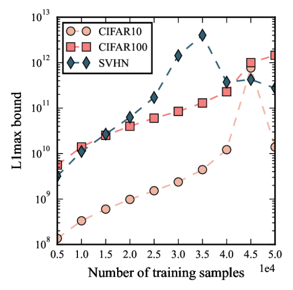
(a)

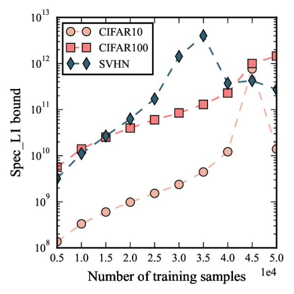
(b)

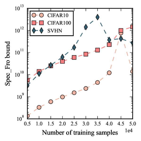
(c)

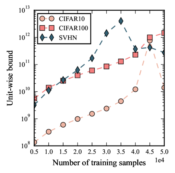
(d)

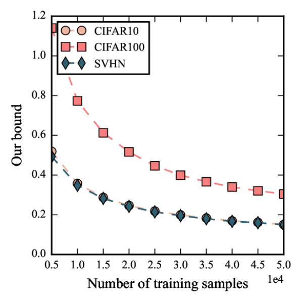
(e)

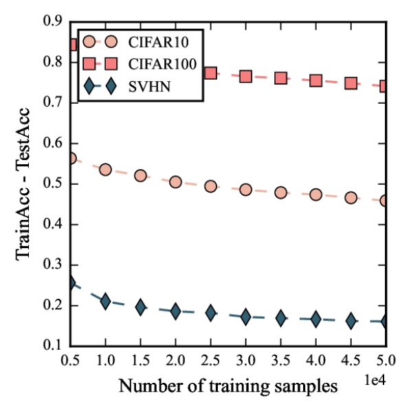
(f)

Figure 2: Comparison between the norm-based generalization measures from (a) Bartlett and Mendelson (2002), (b) Bartlett et al. (2017), (c) Neyshabur et al. (2018), (d) Neyshabur et al. (2019) and (e) our proposed bound on fully connected networks. The subplot (f) depicts the empirical generalization gap (training accuracy minus testing accuracy). The training set size equally ranges from $5\text{\times}{10}^{3}$ to $5\text{\times}{10}^{4}$ with a step size of $5\text{\times}{10}^{3}$ for CIFAR10 (peach) and CIFAR100 (salmon). The lines for SVHN (teal) are normalized to fit the plot due to the mismatch in the size of the training sets.

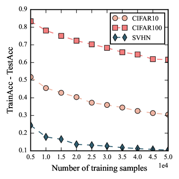
(a)

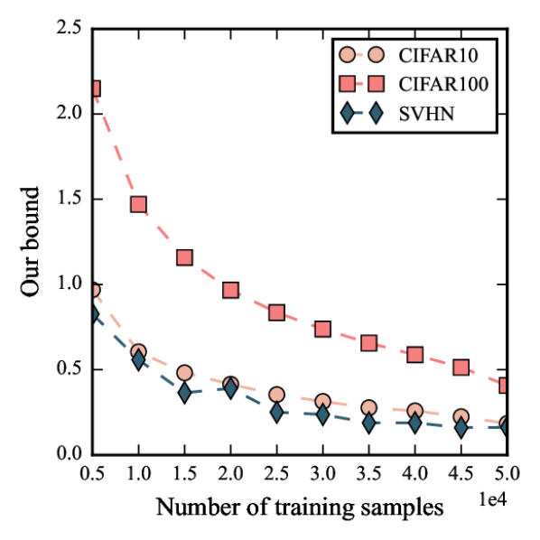
(b)

Figure 3: Generalization gap (a) and our proposed bound (b) for different training set sizes on ResNet18. The training set size equally ranges from $5\text{\times}{10}^{3}$ to $5\text{\times}{10}^{4}$ with a step size of $5\text{\times}{10}^{3}$ for CIFAR10 (peach) and CIFAR100 (salmon). The lines for SVHN (teal) are normalized to fit the plot due to the mismatch in the size of the training sets.

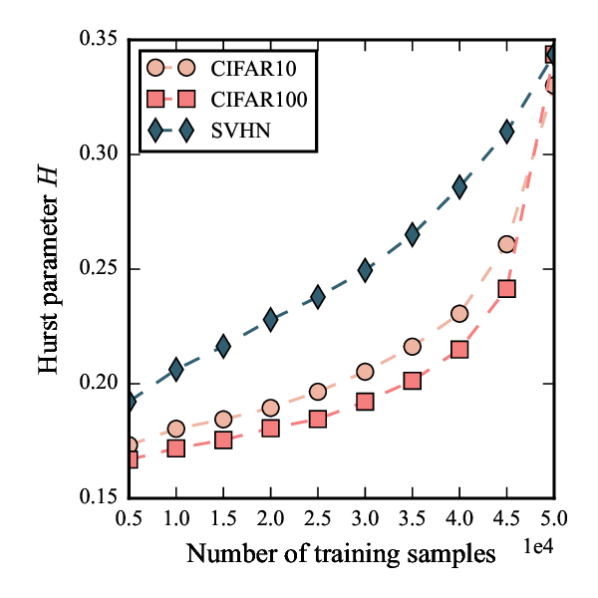
(a) ResNet18

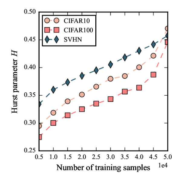
(b) VGG16

Figure 4: Estimation of the Hurst parameter $H$ on (a) ResNet18 and (b) VGG16 for different training set sizes. The training set size equally ranges from $5\text{\times}{10}^{3}$ to $5\text{\times}{10}^{4}$ with a step size of $5\text{\times}{10}^{3}$ for CIFAR10 (peach) and CIFAR100 (salmon). The lines for SVHN (teal) are normalized to fit the plot due to the mismatch in the size of the training sets.

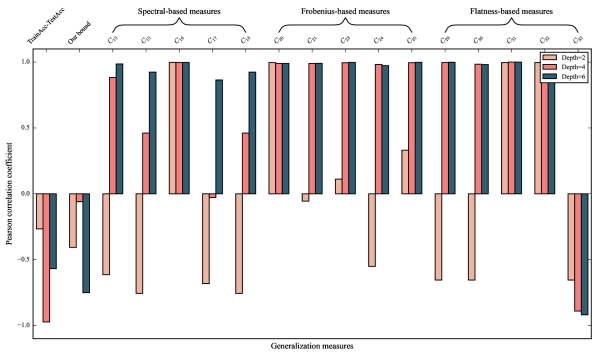
(a) Width

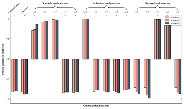
(b) Depth

Figure 5: Effects of varying the width and the depth of the NiN model architecture on SVHN. The x-axis displays three typical types of generalization measures that are excerpted from Dziugaite et al. (2020). The subscript indicates the corresponding equation number in its appendix. The empirical generalization gap (first bar) and our proposed bound (second bar) are also illustrated. The y-axis is the Pearson correlation coefficient between the generalization measure and the width (depth).

5.1 Effects of Training Set Size

Generically, increasing the training set size will boost the generalization performance of DNNs and exhibit an extensive power-law regime of learning curves (Hestness et al., 2017; Spigler et al., 2019; Kaplan et al., 2020; Henighan et al., 2020). As stated before, a wide variety of norm-based bounds nevertheless increase with the training set size (Nagarajan and Kolter, 2019), which has been largely ignored by previous studies. Although a generalization bound that correlates well with the generalization error has been derived (Kuzborskij and Lampert, 2018), it is designed only for one-pass SGD, which is impractical in real scenarios. Recently, a marginal-likelihood PAC-Bayesian bound which, though limited to binary classification, exhibits correct correlation with the training set size is also proposed (Valle-Pérez and Louis, 2020).

Intuitively, it is much easier for DNNs to model a smaller subset of the training set. One may anticipate that SGD will end in local minima that are not far away from the initialization in a short period. By contrast, to model a larger subset, DNNs will spend more time searching for flat minima and move further from the initialization. To verify this intuition, we train models with ten different training set sizes, ranging from $5\text{\times}{10}^{3}$ to $5\text{\times}{10}^{4}$ with a step size of $5\text{\times}{10}^{3}$ for CIFAR10 and CIFAR100. As for SVHN, we also gradually increase the number of training examples with a tenth of the training set every time.

We compare our approach with the covering number bound (Bartlett et al., 2017), the PAC-Bayesian bound (Neyshabur et al., 2018), and two kinds of Rademacher complexity based bounds (Bartlett and Mendelson, 2002; Neyshabur et al., 2019). We must clarify, although we only focus on these four generalization bounds, the conclusion applies to other norm-based bounds as they also depend on the norms that appear in these four bounds, which have been shown to increase with the training set size (Nagarajan and Kolter, 2019).

To start with, we consider a simple fully connected network that consists of only one hidden layer with $1,024$ neurons. As shown in Figure 2, our bound follows the same trend as the generalization gap, while the other bounds display a negative correlation with the training set size. To further validate this observation, we conduct the same experiments with ResNet18 and VGG16. The results are plotted in Figure 3 and 11 and they display a similar trend as well. We also plot the Hurst parameter for these two different model architectures in Figure 4. It clearly illustrates that the estimated Hurst parameter grows with the training set size, implying that increasing the training set size will lead SGD to end in flat minima (Hochreiter and Schmidhuber, 1997; Keskar et al., 2017; Tan et al., 2021).

5.2 Effects of Width and Depth

In this section, we compare our proposed bound against three typical classes of generalization measures that are excerpted from a large-scale empirical study (Dziugaite et al., 2020). The first class of generalization measures is the spectral-based measure, which characterizes the generalization bound in terms of the spectral norm of the weight matrices (Pitas et al., 2018; Neyshabur et al., 2018; Bartlett et al., 2017). The second class is the Frobenius-based measure, which is similar to the first class but uses the Frobenius norm instead (Neyshabur et al., 2015; Jiang et al., 2020). The last class is the flatness-based measure, which connects the flatness of a solution to the generalization through the PAC-Bayesian framework (McAllester, 1999). For each class of generalization measures, we only choose 5 different measures in our study. For convenience, we will refer to each generalization measure according to its equation number appearing in the appendix of Dziugaite et al. (2020).

Since most of the generalization measures cannot be applied to modern network architectures such as skip connection and attention mechanism, we are not able to make use of the most successful model architecture, such as ResNets for a fair comparison. Following the same experimental configuration of Jiang et al. (2020) and Dziugaite et al. (2020), we only focus on a fully convolutional Network-in-Network (NiN), which has achieved reasonably competitive performance on image classification tasks. The model is constructed by stacking multiple blocks, each of which consists of 3 convolutional layers. We can alter the model size by changing the number of blocks (depth) or the number of filters at each convolutional layer (width). In our experiments, we vary the depth from $2$ to $7$ and the width from $6\times 25$ to $16\times 25$.

To better illustrate the effects of varying the width and depth, we calculate the corresponding Pearson correlation coefficient. As shown in the first bar of Figure 5(a), the Pearson correlation coefficient between the empirical generalization gap and the width is negative, indicating that a wider network leads to a smaller generalization gap. This is reasonable since a wider network has more parameters and is more capable in terms of expressivity. The same finding is also true when changing the depth of the network, which can be verified in Figure 5(b).

However, as shown in Figure 5(a), most generalization measures appear to change reversely with the generalization gap while varying the width, especially when the network is deep (depth=6). For a shallow network (depth=2), generalization measures from different classes are more likely to predict correctly. When it comes to varying the depth, we find that most generalization measures can follow the correct trend with the generalization gap, as shown in Figure 5(b). As a comparison, our bound follows the same trend as the generalization gap when changing the width or depth of the network in most cases. Similar observations can also be found for CIFAR10 and CIFAR100, see Figure 14 and 15. Apart from our proposed bound, we find that the flatness-based measure $C_{33}$ (last bar) also correlates well with the empirical generalization gap. In contrast to other flatness-based generalization measures, $C_{33}$ is parameter-dependent and it may suggest that the flatness of the local minima is determined not only by the largest eigenvalue direction but also by the rest of the dimensions. This happens to coincide with the fact that the Hurst parameter is also an average measure of the raggedness of the optimization trajectory.

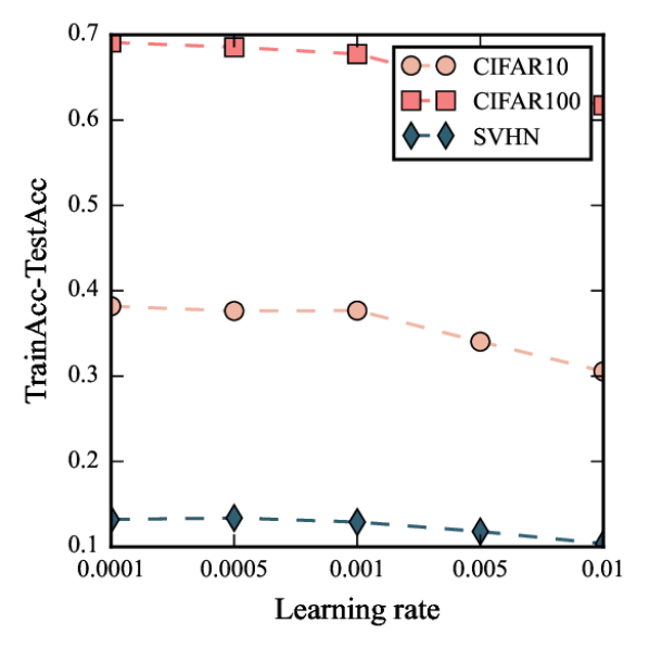
(a)

(b)

Figure 6: Generalization gap (a) and our proposed bound (b) on ResNet18 for different learning rates.

(a)

(b)

Figure 7: Generalization gap (a) and our proposed bound (b) on ResNet18 for different mini-batch sizes.

5.3 Effects of Learning Rate and Mini-batch Size

Another issue that hinders norm-based bounds from wide usage is that they often anti-correlate with the generalization error when changing the commonly used training hyperparameters (Jiang et al., 2020). In this section, we only consider the learning rate and mini-batch size, which typically dominate the generalization performance of different model architectures. We first investigate the effects of varying the learning rate, which ranges in {$1\text{\times}{10}^{-4}$, $5\text{\times}{10}^{-4}$, $1\text{\times}{10}^{-3}$, $5\text{\times}{10}^{-3}$, $1\text{\times}{10}^{-2}$}. Figure 6 exhibits a promising result that our bound decreases with the learning rate, and follows the same trend as the generalization gap.

The effects of varying the mini-batch size are investigated using a sweep $\{32,64,\ldots,2048\}$. As depicted in Figure 7, large mini-batch size usually corresponds to poor generalization.

(a) Vanilla SGD

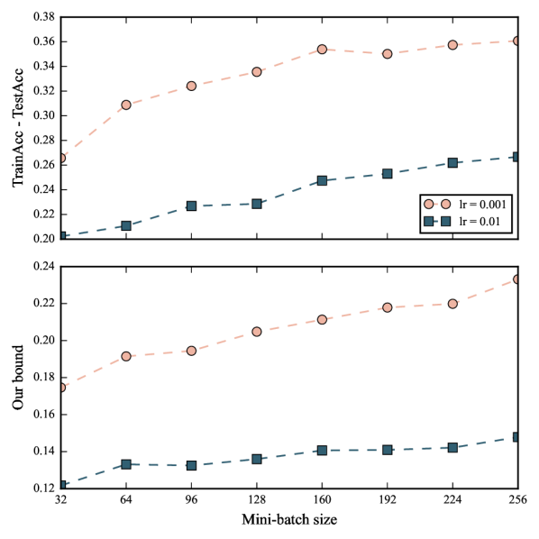
(b) Momentum

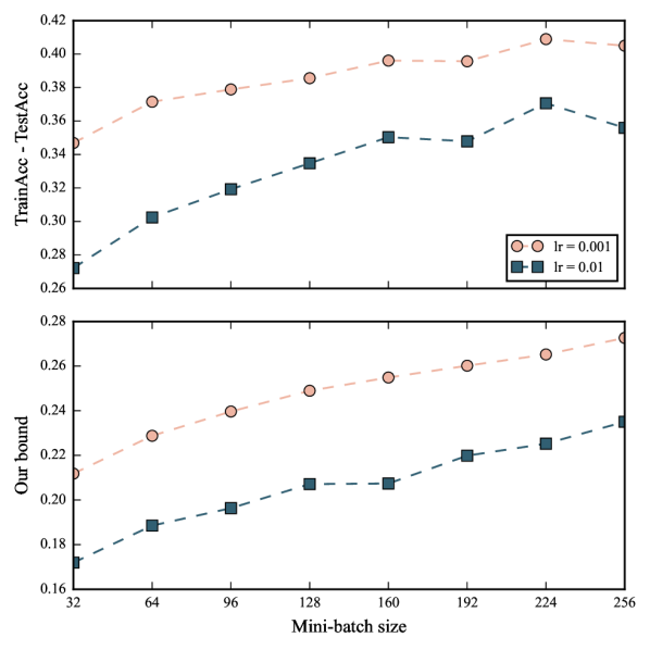
(c) Weight decay

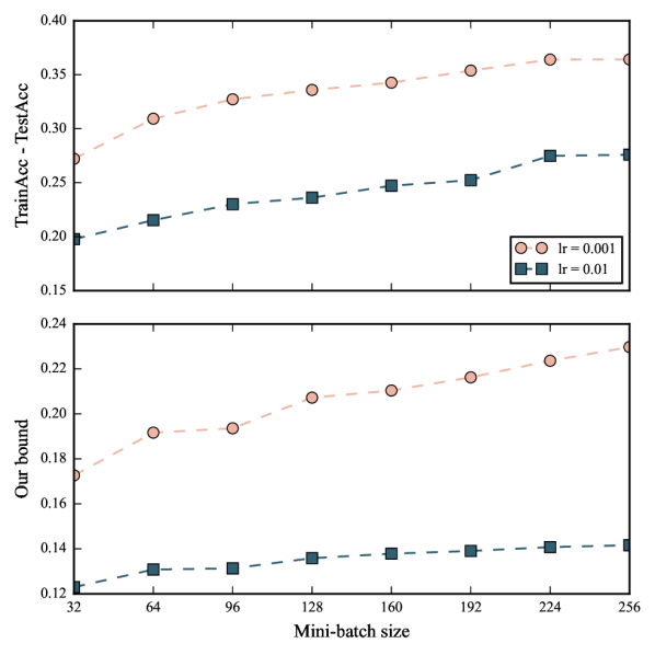
(d) Momentum & Weight decay

Figure 8: Effects of momentum and weight decay on generalization gap (upper panel) and our proposed bound (lower panel) by changing the mini-batch size and learning rate.

5.4 Effects of Momentum and Weight Decay

Though our theoretical analysis is based on vanilla SGD, we also investigate the impacts of momentum and weight decay as both of them are indispensable ingredients to achieving better results. To reveal the influence of different training strategies, we train ResNet18 on CIFAR10 with mini-batches from $\{32,64,\ldots,256\}$ and learning rates from {$1\text{\times}{10}^{-3}$, $1\text{\times}{10}^{-2}$}. We choose the coefficient of momentum as $0.9$ and set the weight decay to a value of $1\text{\times}{10}^{-4}$. As can be seen in Figure 8, the findings of our bound on mini-batch size and learning rate for vanilla SGD are still true in this context: a larger learning rate or a smaller mini-batch size generally leads to a smaller generalization gap. It is noteworthy that momentum is more effective in reducing the generalization gap than weight decay if we compare the results of Figure 8 (a)-(c). And this subtle difference is also captured by our bound.

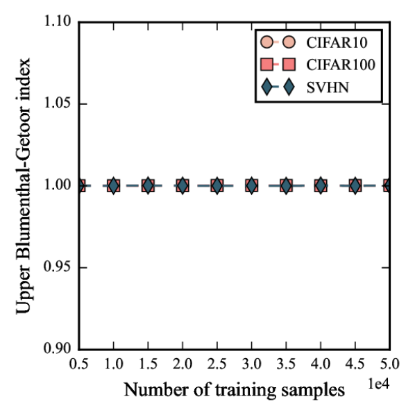
(a)

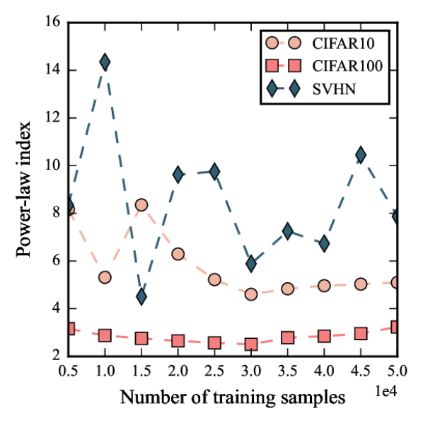
(b)

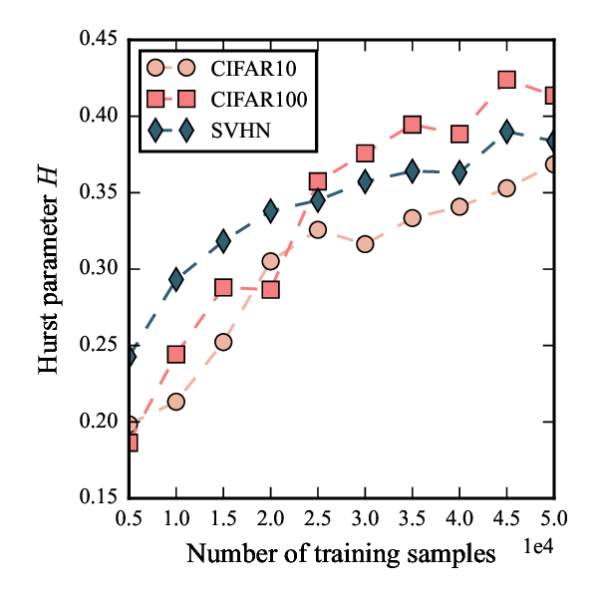
(c)

Figure 9: The effects of changing training set size on (a) upper Blumenthal-Getoor index from Simsekli et al. (2020), (b) power-law index from Mahoney and Martin (2019) and (c) Hurst parameter. The training set size equally ranges from $5\text{\times}{10}^{3}$ to $5\text{\times}{10}^{4}$ with a step size of $5\text{\times}{10}^{3}$ for CIFAR10 (peach) and CIFAR100 (salmon). The lines for SVHN (teal) are normalized to fit the plot due to the mismatch in the size of the training sets.

5.5 Comparison with Existing Generalization Indicators

In this section, we empirically compare the Hurst parameter against existing generalization indicators developed for DNNs. Still, we monitor how the indicators change with the training set size. As the first comparison, we consider the upper Blumenthal-Getoor index (Simsekli et al., 2020), which describes the tailedness of SGN. Another indicator is the power-law index (Mahoney and Martin, 2019), characterizing the empirical spectral density of weight matrices. Ideally, these two indicators would suggest a better generalization if they are smaller. We consider a fully connected network consisting of 4 hidden layers with $1,024$ neurons at each layer. Except for ReLU activation, no other techniques such as dropout or batch normalization are employed. As illustrated in Figure 9, the upper Blumenthal-Getoor index stays around $1.0$ and is non-informative about the training set size. Though the power-law index is sensitive to the training set size, it fails to convey any meaningful information. Meanwhile, the Hurst parameter $H$ gradually increases, implying that increasing training set size will encourage the SGD optimizer to end in flat minima (Tan et al., 2021).

6 Conclusion

Based on the Rademacher complexity of the optimization trajectory picked by SGD, we propose a novel generalization bound from the perspective of fractal geometry, which is different from the norm-based generalization bounds. Empirical results suggest that the proposed bound predicts well the generalization gap over the commonly used experimental interventions, including increasing the training set size, varying the model architecture, and adjusting the choices of training hyperparameters such as learning rate and mini-batch size. Moreover, the Hurst parameter has proved superior to existing generalization indicators such as the power-law index and the upper Blumenthal-Getoor index. Although our theoretical analysis is based on vanilla SGD, empirical evidence suggests that the findings also hold for SGD with momentum and weight decay. Following this line, it would be highly recommended to investigate the impacts of different model ingredients such as skip connection and attention mechanism, and different training strategies, such as Adam and RMSprop. Besides, due to the existence of a break-even point in the first few epochs (Jastrzebski et al., 2020), it is intriguing to study the Hurst parameter in the early phase of SGD dynamics and relate it to the generalization.

Acknowledgments

We would like to give special thanks to the anonymous reviewers, who have suggested numerous improvements in the earlier versions of the manuscript. This work is supported in part by the National Key Research and Development Program of China under Grant 2020AAA0105601 and in part by the National Natural Science Foundation of China under Grants 61976174 and 61877049.

A Robustness of Hurst Parameter

Since large neural networks such as ResNets contain millions of parameters, it is computationally infeasible to estimate the Hurst parameter from the overall parameters. In the experiments, we only use a small random portion of the parameters to estimate the Hurst parameter $H$. To demonstrate this approach is robust, here we use different numbers of parameters to estimate the Hurst parameter, ranging from $1\text{\times}{10}^{4}$ to $11\text{\times}{10}^{6}$ with a step size of $2\text{\times}{10}^{5}$. As shown in Figure 10, the Hurst parameter is insensitive to the number of parameters we use to estimate it. This finding allows us to use only a small random portion, say $5\text{\times}{10}^{4}$, in our experiments without performance degradation.

B Additional Figures

To avoid clutter, several figures are deferred to this section, including experimental results using VGG16 (Figure 11, 12, and 13) and effects of changing width and depth of NiN architecture on CIFAR10 and CIFAR100 (Figure 14 and 15).

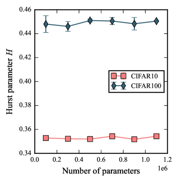
(a)

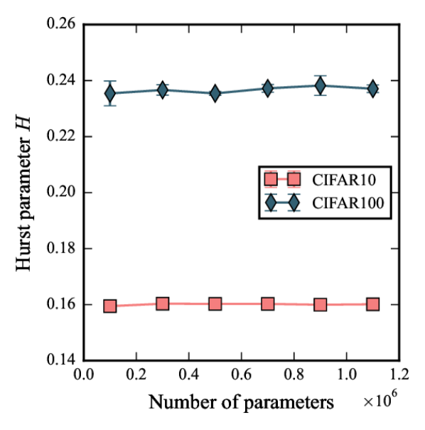
(b)

Figure 10: Hurst parameter estimations for (a) mini-batch size=64 and (b) mini-batch size=512 with different numbers of parameters. The model we use is ResNet18 and the data sets to which we apply are CIFAR10 and CIFAR100. The mean and standard deviation are plotted with three random seeds.

(a)

(b)

Figure 11: Generalization gap (a) and our proposed bound (b) for different training set sizes on VGG16. The training set size equally ranges from $5\text{\times}{10}^{3}$ to $5\text{\times}{10}^{4}$ with a step size of $5\text{\times}{10}^{3}$ for CIFAR10 (peach) and CIFAR100 (salmon). The lines for SVHN (teal) are normalized to fit the plot due to the mismatch in the size of the training sets.

(a)

(b)

Figure 12: Generalization gap (a) and our proposed bound (b) on VGG16 for different learning rates.

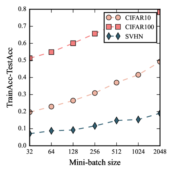
(a)

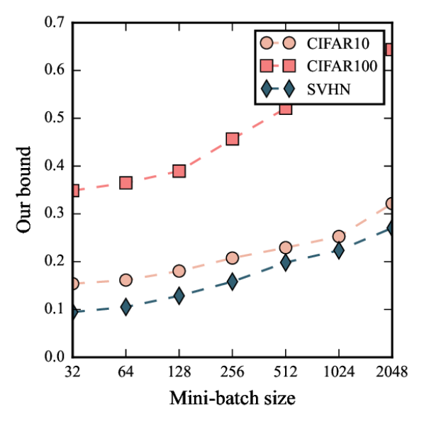
(b)

Figure 13: Generalization gap (a) and our proposed bound (b) on VGG16 for different mini-batch sizes.

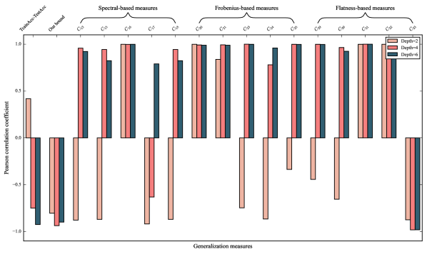
(a) Width

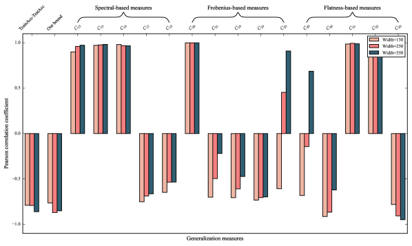
(b) Depth

Figure 14: Effects of varying the width and the depth of the NiN model architecture on CIFAR10. The x-axis displays three typical types of generalization measures that are excerpted from Dziugaite et al. (2020). The subscript indicates the corresponding equation number in its appendix. The empirical generalization gap (first bar) and our proposed bound (second bar) are also illustrated. The y-axis is the Pearson correlation coefficient between the generalization measure and the width (depth).

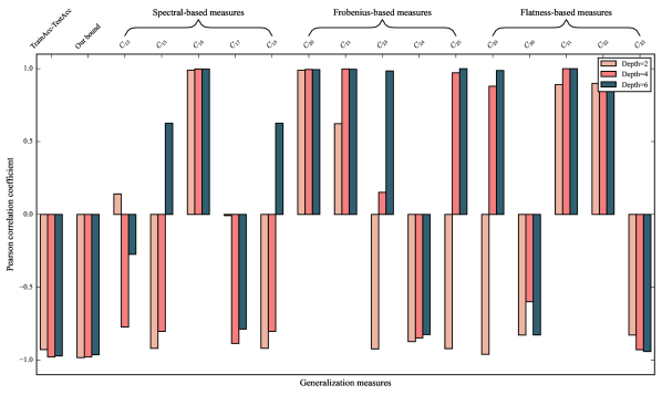
(a) Width

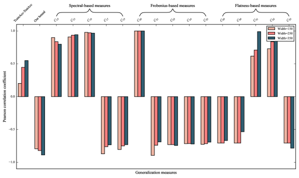
(b) Depth

Figure 15: Effects of varying the width and the depth of the NiN model architecture on CIFAR100. The x-axis displays three typical types of generalization measures that are excerpted from Dziugaite et al. (2020). The subscript indicates the corresponding equation number in its appendix. The empirical generalization gap (first bar) and our proposed bound (second bar) are also illustrated. The y-axis is the Pearson correlation coefficient between the generalization measure and the width (depth).

References

- Arora et al. (2018) S. Arora, R. Ge, B. Neyshabur, and Y. Zhang. Stronger generalization bounds for deep nets via a compression approach. In Proceedings of the 35th International Conference on Machine Learning, pages 254–263, 2018.
- Arora et al. (2019) S. Arora, S. S. Du, W. Hu, Z. Li, and R. Wang. Fine-grained analysis of optimization and generalization for overparameterized two-layer neural networks. In Proceedings of the 36th International Conference on Machine Learning, pages 322–332, 2019.
- Bach and Moulines (2011) F. R. Bach and E. Moulines. Non-asymptotic analysis of stochastic approximation algorithms for machine learning. In Proceedings of the 25th Conference on Neural Information Processing Systems, pages 451–459, 2011.
- Banerjee et al. (2020) A. Banerjee, T. Chen, and Y. Zhou. De-randomized PAC-Bayes margin bounds: Applications to non-convex and non-smooth predictors. ArXiv preprint, abs/2002.09956, 2020.
- Barrett and Dherin (2021) D. G. T. Barrett and B. Dherin. Implicit gradient regularization. In Proceedings of the 9th International Conference on Learning Representations, pages 1–25, 2021.
- Barron and Klusowski (2019) A. R. Barron and J. M. Klusowski. Complexity, statistical risk, and metric entropy of deep nets using total path variation. ArXiv preprint, abs/1902.00800, 2019.
- Bartlett and Mendelson (2002) P. L. Bartlett and S. Mendelson. Rademacher and Gaussian complexities: Risk bounds and structural results. Journal of Machine Learning Research, 3:463–482, 2002.
- Bartlett et al. (2017) P. L. Bartlett, D. J. Foster, and M. Telgarsky. Spectrally-normalized margin bounds for neural networks. In Proceedings of the 31st Conference on Neural Information Processing Systems, pages 6240–6249, 2017.
- Bousquet and Elisseeff (2002) O. Bousquet and A. Elisseeff. Stability and generalization. Journal of Machine Learning Research, 2:499–526, 2002.
- Cao and Gu (2019) Y. Cao and Q. Gu. Generalization bounds of stochastic gradient descent for wide and deep neural networks. In Proceedings of the 33rd Conference on Neural Information Processing Systems, pages 10835–10845, 2019.
- Chaudhari and Soatto (2018) P. Chaudhari and S. Soatto. Stochastic gradient descent performs variational inference, converges to limit cycles for deep networks. In Proceedings of the 6th International Conference on Learning Representations, pages 1–20, 2018.
- Défossez and Bach (2015) A. Défossez and F. R. Bach. Averaged least-mean-squares: Bias-variance trade-offs and optimal sampling distributions. In Proceedings of the 18th International Conference on Artificial Intelligence and Statistics, pages 1–9, 2015.
- Dinh et al. (2017) L. Dinh, R. Pascanu, S. Bengio, and Y. Bengio. Sharp minima can generalize for deep nets. In Proceedings of the 34th International Conference on Machine Learning, pages 1019–1028, 2017.
- Dziugaite et al. (2020) G. K. Dziugaite, A. Drouin, B. Neal, N. Rajkumar, E. Caballero, L. Wang, I. Mitliagkas, and D. M. Roy. In search of robust measures of generalization. In Proceedings of the 34th Conference on Neural Information Processing Systems, pages 1–28, 2020.
- Falconer (2004) K. Falconer. Fractal Geometry: Mathematical Foundations and Applications. John Wiley & Sons, 2004.
- Foster et al. (2019) D. J. Foster, S. Greenberg, S. Kale, H. Luo, M. Mohri, and K. Sridharan. Hypothesis set stability and generalization. In Proceedings of the 33rd Conference on Neural Information Processing Systems, pages 6726–6736, 2019.
- Golowich et al. (2018) N. Golowich, A. Rakhlin, and O. Shamir. Size-independent sample complexity of neural networks. In Proceedings of the 31st Annual Conference on Learning Theory, pages 297–299, 2018.
- Hardt et al. (2016) M. Hardt, B. Recht, and Y. Singer. Train faster, generalize better: Stability of stochastic gradient descent. In Proceedings of the 33rd International Conference on Machine Learning, pages 1225–1234, 2016.
- Henighan et al. (2020) T. Henighan, J. Kaplan, M. Katz, M. Chen, C. Hesse, J. Jackson, H. Jun, T. B. Brown, P. Dhariwal, S. Gray, et al. Scaling laws for autoregressive generative modeling. ArXiv preprint, abs/2010.14701, 2020.
- Hestness et al. (2017) J. Hestness, S. Narang, N. Ardalani, G. Diamos, H. Jun, H. Kianinejad, M. Patwary, M. Ali, Y. Yang, and Y. Zhou. Deep learning scaling is predictable, empirically. ArXiv preprint, abs/1712.00409, 2017.
- Hirt (1968) C. W. Hirt. Heuristic stability theory for finite-difference equations. Journal of Computational Physics, 2(4):339–355, 1968.
- Hochreiter and Schmidhuber (1997) S. Hochreiter and J. Schmidhuber. Flat minima. Neural Computation, 9(1):1–42, 1997.
- Hu et al. (2017) W. Hu, C. J. Li, L. Li, and J.-G. Liu. On the diffusion approximation of nonconvex stochastic gradient descent. ArXiv preprint, abs/1705.07562, 2017.
- Ioffe and Szegedy (2015) S. Ioffe and C. Szegedy. Batch normalization: Accelerating deep network training by reducing internal covariate shift. In Proceedings of the 32nd International Conference on Machine Learning, pages 448–456, 2015.
- Jacot et al. (2018) A. Jacot, C. Hongler, and F. Gabriel. Neural tangent kernel: Convergence and generalization in neural networks. In Proceedings of the 32nd Conference on Neural Information Processing Systems, pages 8580–8589, 2018.
- Jastrzebski et al. (2017) S. Jastrzebski, Z. Kenton, D. Arpit, N. Ballas, A. Fischer, Y. Bengio, and A. Storkey. Three factors influencing minima in SGD. ArXiv preprint, abs/1711.04623, 2017.
- Jastrzebski et al. (2020) S. Jastrzebski, M. Szymczak, S. Fort, D. Arpit, J. Tabor, K. Cho, and K. Geras. The break-even point on optimization trajectories of deep neural networks. In Proceedings of the 8th International Conference on Learning Representations, pages 1–21, 2020.
- Jiang et al. (2020) Y. Jiang, B. Neyshabur, H. Mobahi, D. Krishnan, and S. Bengio. Fantastic generalization measures and where to find them. In Proceedings of the 8th International Conference on Learning Representations, pages 1–33, 2020.
- Kaplan et al. (2020) J. Kaplan, S. McCandlish, T. Henighan, T. B. Brown, B. Chess, R. Child, S. Gray, A. Radford, J. Wu, and D. Amodei. Scaling laws for neural language models. ArXiv preprint, abs/2001.08361, 2020.
- Kawaguchi et al. (2020) K. Kawaguchi, L. P. Kaelbling, and Y. Bengio. Generalization in deep learning. ArXiv preprint, abs/2010.11924, 2020.
- Keskar et al. (2017) N. S. Keskar, D. Mudigere, J. Nocedal, M. Smelyanskiy, and P. T. P. Tang. On large-batch training for deep learning: Generalization gap and sharp minima. In Proceedings of the 5th International Conference on Learning Representations, pages 1–16, 2017.
- Klingenhöfer and Zähle (1999) F. Klingenhöfer and M. Zähle. Ordinary differential equations with fractal noise. Proceedings of the American Mathematical Society, 127(4):1021–1028, 1999.
- Krizhevsky et al. (2009) A. Krizhevsky, G. Hinton, et al. Learning multiple layers of features from tiny images. Technical report, University of Toronto, 2009.
- Krogh and Hertz (1992) A. Krogh and J. A. Hertz. A simple weight decay can improve generalization. In Proceedings of the 6th Conference on Neural Information Processing Systems, pages 950–957, 1992.
- Kuzborskij and Lampert (2018) I. Kuzborskij and C. H. Lampert. Data-dependent stability of stochastic gradient descent. In Proceedings of the 35th International Conference on Machine Learning, pages 2820–2829, 2018.
- Lee et al. (2019) J. Lee, L. Xiao, S. S. Schoenholz, Y. Bahri, R. Novak, J. Sohl-Dickstein, and J. Pennington. Wide neural networks of any depth evolve as linear models under gradient descent. In Proceedings of the 33rd Conference on Neural Information Processing Systems, pages 8570–8581, 2019.
- Li et al. (2015) Q. Li, C. Tai, and E. Weinan. Dynamics of stochastic gradient algorithms. ArXiv preprint, abs/1511.06251, 2015.
- Li et al. (2017) Q. Li, C. Tai, and W. E. Stochastic modified equations and adaptive stochastic gradient algorithms. In Proceedings of the 34th International Conference on Machine Learning, pages 2101–2110, 2017.
- Li et al. (2019) Q. Li, C. Tai, and E. Weinan. Stochastic modified equations and dynamics of stochastic gradient algorithms i: Mathematical foundations. Journal of Machine Learning Research, 20:40–1, 2019.
- Li et al. (2021) Z. Li, S. Malladi, and S. Arora. On the validity of modeling SGD with stochastic differential equations (SDEs). ArXiv preprint, abs/2102.12470, 2021.
- Littlestone and Warmuth (1986) N. Littlestone and M. Warmuth. Relating data compression and learnability. Technical report, University of California Santa Cruz, 1986.
- Lou and Ouyang (2016) S. Lou and C. Ouyang. Fractal dimensions of rough differential equations driven by fractional Brownian motions. Stochastic Processes and their Applications, 126(8):2410–2429, 2016.
- Mahoney and Martin (2019) M. W. Mahoney and C. Martin. Traditional and heavy tailed self regularization in neural network models. In Proceedings of the 36th International Conference on Machine Learning, pages 4284–4293, 2019.
- Mandelbrot and Van Ness (1968) B. B. Mandelbrot and J. W. Van Ness. Fractional Brownian motions, fractional noises and applications. SIAM Review, 10(4):422–437, 1968.
- Mandt et al. (2017) S. Mandt, M. D. Hoffman, and D. M. Blei. Stochastic gradient descent as approximate Bayesian inference. Journal of Machine Learning Research, 18:1–35, 2017.
- Mattila (1999) P. Mattila. Geometry of Sets and Measures in Euclidean Spaces: Fractals and Rectifiability. Cambridge University Press, 1999.
- McAllester (1999) D. A. McAllester. PAC-Bayesian model averaging. In Proceedings of the 12nd Annual Conference on Computational learning theory, pages 164–170, 1999.
- McDiarmid et al. (1989) C. McDiarmid et al. On the method of bounded differences. Surveys in combinatorics, 141(1):148–188, 1989.
- Mishura and Shevchenko (2008) Y. Mishura and G. Shevchenko. The rate of convergence for Euler approximations of solutions of stochastic differential equations driven by fractional Brownian motion. Stochastics, 80(5):489–511, 2008.
- Mohri et al. (2018) M. Mohri, A. Rostamizadeh, and A. Talwalkar. Foundations of Machine Learning. MIT Press, 2018.
- Mou et al. (2018) W. Mou, L. Wang, X. Zhai, and K. Zheng. Generalization bounds of SGLD for non-convex learning: Two theoretical viewpoints. In Proceedings of the 31st Conference On Learning Theory, pages 605–638, 2018.
- Nagarajan and Kolter (2019) V. Nagarajan and J. Z. Kolter. Uniform convergence may be unable to explain generalization in deep learning. In Proceedings of the 33rd Conference on Neural Information Processing Systems, pages 11611–11622, 2019.
- Needell et al. (2014) D. Needell, R. Ward, and N. Srebro. Stochastic gradient descent, weighted sampling, and the randomized Kaczmarz algorithm. In Proceedings of the 28th Conference on Neural Information Processing Systems, pages 1017–1025, 2014.
- Netzer et al. (2011) Y. Netzer, T. Wang, A. Coates, A. Bissacco, B. Wu, and A. Y. Ng. Reading digits in natural images with unsupervised feature learning. In Proceedings of the 25th Conference on Neural Information Processing Systems, Workshop on Deep Learning and Unsupervised Feature Learning, pages 1–9, 2011.
- Neyshabur et al. (2015) B. Neyshabur, R. Tomioka, and N. Srebro. Norm-based capacity control in neural networks. In Proceedings of the 28th Conference on Learning Theory, pages 1376–1401, 2015.
- Neyshabur et al. (2017) B. Neyshabur, S. Bhojanapalli, D. McAllester, and N. Srebro. Exploring generalization in deep learning. In Proceedings of the 31st Conference on Neural Information Processing Systems, pages 5947–5956, 2017.
- Neyshabur et al. (2018) B. Neyshabur, S. Bhojanapalli, and N. Srebro. A PAC-Bayesian approach to spectrally-normalized margin bounds for neural networks. In Proceedings of the 6th International Conference on Learning Representations, pages 1–9, 2018.
- Neyshabur et al. (2019) B. Neyshabur, Z. Li, S. Bhojanapalli, Y. LeCun, and N. Srebro. The role of over-parametrization in generalization of neural networks. In Proceedings of the 7th International Conference on Learning Representations, pages 1–19, 2019.
- Nguyen et al. (2019) T. H. Nguyen, U. Simsekli, M. Gürbüzbalaban, and G. Richard. First exit time analysis of stochastic gradient descent under heavy-tailed gradient noise. In Proceedings of the 33rd Conference on Neural Information Processing Systems, pages 273–283, 2019.
- Noh and Protter (1963) W. Noh and M. Protter. Difference methods and the equations of hydrodynamics. Journal of Mathematics and Mechanics, 12(2):149–191, 1963.
- Panigrahi et al. (2019) A. Panigrahi, R. Somani, N. Goyal, and P. Netrapalli. Non-Gaussianity of stochastic gradient noise. In Proceedings of The 33rd Conference on Neural Information Processing Systems, Workshop on Science Meets Engineering of Deep Learning, pages 1–10, 2019.
- Pitas et al. (2018) K. Pitas, M. Davies, and P. Vandergheynst. PAC-Bayesian margin bounds for convolutional neural networks. ArXiv preprint, abs/1801.00171, 2018.
- Shalev-Shwartz and Ben-David (2014) S. Shalev-Shwartz and S. Ben-David. Understanding Machine Learning: From Theory to Algorithms. Cambridge University Press, 2014.
- Simsekli et al. (2019) U. Simsekli, L. Sagun, and M. Gürbüzbalaban. A tail-index analysis of stochastic gradient noise in deep neural networks. In Proceedings of the 36th International Conference on Machine Learning, pages 5827–5837, 2019.
- Simsekli et al. (2020) U. Simsekli, O. Sener, G. Deligiannidis, and M. A. Erdogdu. Hausdorff dimension, heavy tails, and generalization in neural networks. In Proceedings of the 34th Conference on Neural Information Processing Systems, pages 1–14, 2020.
- Smith et al. (2020) S. L. Smith, E. Elsen, and S. De. On the generalization benefit of noise in stochastic gradient descent. In Proceedings of the 37th International Conference on Machine Learning, pages 9058–9067, 2020.
- Smith et al. (2021) S. L. Smith, B. Dherin, D. G. T. Barrett, and S. De. On the origin of implicit regularization in stochastic gradient descent. In Proceedings of the 9th International Conference on Learning Representations, pages 1–14, 2021.
- Spigler et al. (2019) S. Spigler, M. Geiger, and M. Wyart. Asymptotic learning curves of kernel methods: empirical data vs teacher-student paradigm. ArXiv preprint, abs/1905.10843, 2019.
- Tan et al. (2021) C. Tan, J. Zhang, and J. Liu. Understanding short-range memory effects in deep neural networks. ArXiv preprint, abs/2105.02062, 2021.
- Valle-Pérez and Louis (2020) G. Valle-Pérez and A. A. Louis. Generalization bounds for deep learning. ArXiv preprint, abs/2010.11924, 2020.
- Vapnik (1999) V. Vapnik. The Nature of Statistical Learning Theory. Springer Science & Business Media, 1999.
- Vapnik and Chervonenkis (1971) V. Vapnik and A. Chervonenkis. On the uniform convergence of relative frequencies of events to their probabilities. Theory of Probability & Its Applications, 16(2):264–280, 1971.
- Warming and Hyett (1974) R. Warming and B. Hyett. The modified equation approach to the stability and accuracy analysis of finite-difference methods. Journal of Computational Physics, 14(2):159–179, 1974.
- Xie et al. (2021) Z. Xie, I. Sato, and M. Sugiyama. A diffusion theory for deep learning dynamics: Stochastic gradient descent escapes from sharp minima exponentially fast. In Proceedings of the 9th International Conference on Learning Representations, pages 1–28, 2021.
- Yaida (2019) S. Yaida. Fluctuation-dissipation relations for stochastic gradient descent. In Proceedings of the 7th International Conference on Learning Representations, pages 1–15, 2019.
- Zhang et al. (2017) C. Zhang, S. Bengio, M. Hardt, B. Recht, and O. Vinyals. Understanding deep learning requires rethinking generalization. In Proceedings of the 5th International Conference on Learning Representations, pages 1–15, 2017.
- Zhang et al. (2020) J. Zhang, S. P. Karimireddy, A. Veit, S. Kim, S. Reddi, S. Kumar, and S. Sra. Why are adaptive methods good for attention models? In Proceedings of the 34th Conference on Neural Information Processing Systems, pages 1–23, 2020.
- Zhu et al. (2019) Z. Zhu, J. Wu, B. Yu, L. Wu, and J. Ma. The anisotropic noise in stochastic gradient descent: Its behavior of escaping from sharp minima and regularization effects. In Proceedings of the 36th International Conference on Machine Learning, pages 7654–7663, 2019.