A Multiwavelength Study of the Sgr B Region: Contiguous Cloud-Cloud Collisions Triggering Widespread Star Formation Events?

Abstract

The Sgr B region, including Sgr B1 and Sgr B2, is one of the most active star-forming regions in the Galaxy. Hasegawa et al. (1994) originally proposed that Sgr B2 was formed by a cloud-cloud collision (CCC) between two clouds with velocities of $\sim$45 km s^-1 and $\sim$75 km s^-1. However, some recent observational studies conflict with this scenario. We have re-analyzed this region, by using recent, fully sampled, dense-gas data and by employing a recently developed CCC identification methodology, with which we have successfully identified more than 50 CCCs and compared them at various wavelengths. We found two velocity components that are widely spread across this region and that show clear signatures of a CCC, each with a mass of $\sim$10⁶ M_⊙. Based on these observational results, we suggest an alternative scenario, in which contiguous collisions between two velocity features with a relative velocity of $\sim$20 km s^-1 created both Sgr B1 and Sgr B2. The physical parameters, such as the column density and the relative velocity of the colliding clouds, satisfy a relation that has been found to apply to the most massive Galactic CCCs, meaning that the triggering of high-mass star formation in the Galaxy and starbursts in external galaxies can be understood as being due to the same physical CCC process.

1 Introduction

1.1 The Center of the Galaxy

Despite its small volume, the inner 1 kpc of the Galaxy contains several to 10$\%$ of molecular gas, and thus it is a prominent mass reservoir (Morris & Serabyn, 1996). As expected from the large amount of gas, the strength of the frozen-in magnetic fields is very high in the Galactic Center (GC). It has been estimated to be at least 30 $\mu$G (Crocker et al., 2010) and this leads to very large Alfvén speeds of a few tens to a hundred km s^-1. Thus, the nonnegligible field can accelerate gas, and this makes the situation more complicated in the GC (Fukui et al., 2006).

Molecular-line observations have revealed that the molecular gas in the GC exhibits a very large velocity width and a parallelogram shape in the $l$–$v$ diagram, which cannot be explained by Galactic rotation (e.g., Oka et al., 1998; Tsuboi et al., 1999). The acceleration mechanism of the gas is still unclear, but so far two possible accelerators have been suggested.

One is the bar potential, originally proposed by Binney et al. (1991). They suggested that the framework of the parallelogram in the $l$–$v$ diagram is explained by the innermost orbits of the so-called $x_{1}$ orbits. However, there has been no firm observational evidence of the small bar, which is required to fit the size of the parallelogram to the observed one. Furthermore, many recent theoretical and observational works have revealed that the bar is much larger and rotates at a much slower pattern speed than assumed in Binney et al. (1991) (see e.g., Wegg & Gerhard, 2013; Sormani et al., 2015; Portail et al., 2017; Sanders et al., 2019).

In accordance with those findings, Fux (1999) performed simulations using a composite $N$-body and hydro code, and exhibited asymmetric and non-stationary gas flows that substantially reproduce the observed $l$–$v$ diagrams of Hi and CO. Recent hydrodynamic simulations by Rodríguez-Fernández (2011) and Sormani et al. (2018) have successfully explained the lateral sides of the parallelogram as dust lanes or gas that has been collisionally accelerated by dust lanes. On the other hand, the top and bottom sides of the parallelogram are still unclear. Although Sormani et al. (2018) have interpreted them as brushed gas between the dust lanes and the central molecular zone (CMZ), the boundaries of the top and bottom sides in the simulations still remain obscured and are not so clear compared to the CO emissions seen in Oka et al. (1998).

The other acceleration mechanism involves magnetic instabilities, such as the magnetorotational instability and Parker instability originally proposed by Fukui et al. (2006). Some magnetohydrodynamic (MHD) simulations have revealed that this mechanism can also accelerate gas and can reproduce a parallelogram-like distribution as a transient feature (e.g., Suzuki et al., 2015), although the shape is blobby and not clear. This model also has observational difficulty. Obtaining a direct detection of the magnetic field embedded in the dense molecular gas with a large line width is fairly difficult, so there have been few works that have tackle the situation through a new method, using far-infrared (FIR) polarimetry and velocity gradients of gas (Hu et al., 2021).

Similar to the acceleration mechanism, many models for the dynamical structure of the molecular condensation within the central 200 pc—hereafter, the CMZ (Morris & Serabyn, 1996)—have been proposed (e.g., an expanding shell—Sofue 1995; a twisted ring—Molinari et al. 2011; and an open orbit—Kruijssen et al. 2015). Regardless of which model is ultimately proven to be correct, revealing the star formation mechanism in the dense molecular cloud in such an extreme magnetized, highly pressured environment is important for our understanding of the Galaxy evolution.

Although the central mass reservoir often acts as a star formation engine, star formation in the GC is inactive compared to the theoretical expectation, and possibly suppressed (e.g., Longmore et al., 2013). In order to unveil this star formation mystery, a multiwavelength study—including both dense- and diffuse-gas tracers—will be important, because the star formation timescale is shortened in such extreme condition by external pressures (Kauffmann, 2016), and hence the dense gas no longer holds information regarding the triggering mechanism. Thanks to the improvement in heterodyne receivers over the last two decades, plenty of molecular line surveys have been carried out (e.g., Jones et al., 2012). However, most works focus only on the main streams of the CMZ, with dense-gas tracers, and do not include the diffuse gas traced by CO. We therefore focus on the most active star forming region in the CMZ, Sgr B, and conduct a multiwavelength study with the latest archival data sets, which cover large area and density range, integrating them with knowledge obtained from previous studies.

1.2 The Sgr B region

The Sgr B region, consisting of Sgr B1 and B2, is one of the brightest radio sources, and is located a projected distance of $\sim$100 pc away from the GC. The Sgr B region is also known to be a strong SiO source in the Galaxy (Martín-Pintado et al., 1997). Mehringer et al. (1992) carried out observations of the radio-continuum and recombination lines toward Sgr B1 using the Very Large Array (VLA), and they found extended emission in Sgr B1, unlike Sgr B2. They discussed the possibility that the emission may have been caused by coalesced, evolved Hii regions, and from the proximities of Sgr B1 and Sgr B2 in terms of their projected distances and revealed ionized gas velocities, they suggested that Sgr B1 and Sgr B2 are a unified structure. Mehringer et al. (1993) investigated OH and H₂O masers toward Sgr B1 using the VLA, and discovered an OH maser and ten H₂O maser spots. These observations provide evidence for ongoing star formation in Sgr B1, although the majority of the radio-continuum emission—or, in other words, the star-forming activity—in this region is dominated by evolved Hii regions. Although estimating a quantitative value for the star-forming activity in the GC region is very difficult, due to the heavy extinction at optical wavelengths, Simpson et al. (2018) found that at least eight separate subregions were highly excited by high-mass stars. From their analyses of the spectral energy distributions obtained from [Oiii] 52 and 88 $\mu$m data, taken with the Stratospheric Observatory for Infrared Astronomy, they concluded that these high-mass stars were equivalent to late O-type stars. They also estimated the ages of those late O-type stars to be at least a few Myr. From analyses of radio-continuum emissions obtained with the Wilkinson Microwave Anisotropy Probe, Barnes et al. (2017) also estimated the total stellar mass embedded within Sgr B1 to be $\sim$8000 M_⊙.

Sgr B2 is young, and it is the most active star-forming region in the Galaxy. It contains numerous O-type stars, Hii regions, ultracompact and compact Hii regions, H₂O masers (e.g., Yusef-Zadeh et al., 2004; McGrath et al., 2004), and also a wealth of chemical species, such as organic molecules. The IR luminosity is incredibly high, $\sim$10⁷ L_⊙ (Goldsmith et al., 1987), and its FIR spectrum and [Cii] 157.7 $\mu$m line are comparable to those in FIR-bright galaxies (Vastel et al., 2002). Almost all of the star-forming activity is concentrated within three regions, with diameters of $\sim$1 pc, called Sgr B2(N), Sgr B2(M), and Sgr B2(S), which are aligned from north to south (Benson & Johnston, 1984). Sgr B2(M) is a notable starburst region that contains 49 ultracompact Hii regions (Gaume et al., 1995). Recently, Ginsburg et al. (2018) carried out 3 mm radio-continuum observations with ALMA, and discovered 271 compact sources, which may consist of hypercompact Hii regions and massive young stellar objects, within a 5 pc radius around Sgr B2(M).

Sgr B2 is associated with a giant molecular cloud containing 6 $\times$ 10⁶ M_⊙ (Lis & Goldsmith, 1989). Sofue (1990) discovered giant molecular complexes associated with Sgr B1 and B2, namely, the Sgr B1 molecular shell and the Sgr B2 molecular complex. He suggested that star formation in Sgr B2 was triggered by a compression induced by the expansion of the Sgr B1 molecular shell, driven by feedback from Sgr B1. On the other hand, Hasegawa et al. (1994) proposed a cloud-cloud collision (hereafter, CCC) scenario for the Sgr B2 region, based on their ¹³CO($J$=1–0) observations with the Nobeyama 45 m telescope. They discovered three clouds in the direction of this region, which they named the Shell, at $V_{LSR}$ = 20–40 km s^-1; the Hole, at $V_{LSR}$ = 40–50 km s^-1; and the Clump, at $V_{LSR}$ = 70–80 km s^-1 (see also Figure 1). They interpreted the Clump, Hole, and Shell as clouds that have been compressed, hollowed, and shocked by the CCC, respectively, and they concluded that massive star formation in the Sgr B2 complex was triggered by the collision. Sato et al. (2000) and Hasegawa et al. (2008) lent further support to this model, by comparing the spatial and velocity distributions of their C¹⁸O($J$=1–0), C¹⁸O($J$=3–2), CS($J$=1–0), and CS($J$=7–6) data sets with those of the masers. However, these models are based on under-sampled datasets, so the effective spatial resolution is low. Also, this scenario conflicts with recent observational results at other wavelengths. By analyzing HNCO data, Henshaw et al. (2016) found that there is only one cloud toward Sgr B2, and they suggested that the cloud identification by Hasegawa et al. (1994) was suspicious. Based on a dynamical model of the CMZ, Kruijssen et al. (2019) suggested that the complex kinematic structure of Sgr B2 was naturally explained by the superimposition of fragmentation and orbital motion of a cloud in the line of sight (LOS).

Although Sgr B2 is the most active star-forming region in the Galaxy, the other active star-forming region that physically connects with it—i.e., Sgr B1—has not been explained together with Sgr B2 in either scenarios. Furthermore, the CCC scenario has been gradually taken into account in recent dynamical models of the CMZ. Sormani et al. (2020) suggested that CCCs were naturally present in their hydrodynamic simulations, thus it is important to examine whether the observational footprints of the CCCs are consistent with those simulations and dynamical models. Therefore, reexamination of the CCC scenario for Sgr B2 based on existing dynamical models is required, and this scenario also needs to be applicable mot only to Sgr B2 but also to Sgr B1.

1.3 CCC and High-mass Star Formation

It is well-known that a starburst in a merger is triggered by a collision between two giant molecular clouds belonging to the two galaxies (see, Young et al., 1986). A CCC is a mechanism that collects gas and magnetic fields at super sonic velocity. Numerical simulations indicate that a CCC produces a compressed layer of gas that generates massive, gravitationally unstable, molecular clumps within it. Owing to the enhancement of the magnetic field strength by shock compression, the clumps have effective Jeans masses large enough to develop into high-mass stars (Habe & Ohta, 1992; Inoue & Fukui, 2013; Inoue et al., 2018). However, it is still unknown how many new stars are triggered by a CCC. In other words, the controlling parameters, which determine the scale of the star-forming activity initiated by a CCC, are still unknown, although they must be related to the initial physical conditions of the collision.

Thanks to recent Galactic plane surveys with 1 pc to subpc resolution—such as those done by the Mopra and Nobeyama 45 m telescopes in CO (Braiding et al., 2018; Umemoto et al., 2017)—the mechanism operating in CCCs have gradually been unveiled. These datasets exhibit many candidate CCCs in the Galaxy; in total, more than 50 Hii regions and star clusters are possible sites of CCCs (e.g., Nishimura et al., 2018; Fukui et al., 2018c, b; Ohama et al., 2018; Enokiya et al., 2018; Kohno et al., 2018; Torii et al., 2018; Sano et al., 2018; Hayashi et al., 2018). Also, nearby extragalactic giant Hii regions, such as NGC 604 in M 33 and R136 in the Large Magellanic Cloud, have been suggested to be the results of large-scale collisions between two giant Hi clouds (Tachihara et al., 2018; Fukui et al., 2017). These results suggest that a CCC may be the major mechanism responsible for triggering high-mass star formation (Fukui et al., 2021).

In order to link our understanding of CCCs in starburst galaxies with those in the Galactic Hii regions, the nearest center of the galaxy—the GC of the Milky Way—is the most important target. The GC has the highest volume density of molecular clouds in the Galaxy, and hence, it is likely to have the highest frequency of CCCs as well (Enokiya & Fukui, 2021). The physical parameters of molecular clouds in the GC, such as their densities and relative velocities, are different from those in the Galactic disk. The GC is thus a suitable region for investigating these control parameters. As a first step for investigating CCCs in the GC, Enokiya et al. (2021a) applied a CCC identification methodology developed by Fukui et al. (2021) to the common footpoint of magnetic loops 1 and 2, and they found two pairs of colliding clouds. Thus, they not only demonstrated the validity of this methodology in the GC, but also determined a unique property only seen in CCCs in the GC: they detected SiO emissions caused by a larger relative velocity of $\sim$a few tens of km s^-1.

1.4 The Aims of This Paper

The CCC scenario in Sgr B2, originally proposed by Hasegawa et al. (1994) and followed by Sato et al. (2000), has attracted much attention. However, there are still some uncertainties, as below. This scenario:

1. selected three velocity clouds by eye, but this is arbitrary;

2. was only based on the distribution of molecular gas, and did not consider other wavelengths;

3. used undersampled data sets;

4. neglected Sgr B1; and

5. did not consider the dynamical structure of the CMZ, leaving the possibility of clouds colliding at the position of Sgr B2 uncertain.

In the present paper, we utilize the CCC identification method recently developed by Fukui et al. (2021) and Enokiya et al. (2021a), employing recent, fully sampled data sets with large enough coverage to include Sgr B1 and large enough density dynamic range to investigate whether the CCC model is still applicable. By comparing the gas distribution and recent high-resolution IR and radio-continuum data, we have constructed a multiwavelength view of the region. We finally discuss the possibility of the CCC event and resulting star formation, together with the dynamical structures of the CMZ.

Sections 2 and 3 provide information about the methodology and data sets used in this paper. Our main results are described in Section 4. Section 5 is divided into three sub-Sections, in which we discuss comparisons with numerical simulations (5.1), a possible scenario based on a CCC (5.2), and comparisons with other CCCs in the Galaxy (5.3). We summaries the present study in Section 6.

2 Methodology

2.1 Signatures of a CCC

In this Section, we first introduce the methodology developed by Fukui et al. (2018a, 2021) and Enokiya et al. (2021a, b) to identify a CCC. This methodology has so far successfully identified more than 50 CCC candidates. Based on synthetic observations of numerical simulations (Takahira et al., 2014; Haworth et al., 2015) and on observational data of the Galactic Hii regions, Fukui et al. (2021) proposed the following signatures of a CCC;

1. Complementary distributions between two colliding clouds: a larger cloud is hollowed out by a smaller cloud during a collision and forms the complementary spatial signature. This signature is sometimes accompanied by a spatial displacement, depending on the inclination angle of the relative motion to the LOS.

2. A V-shaped structure or bridge feature in the position-velocity diagram: In the early stage of a CCC, the contact surface between the two clouds forms bridge features by exchanging momenta. This signature develops into a V-shaped structure when the larger cloud is hollowed out.

3. Positional coincidence between the compressed layer and the high-mass star-forming region.

However, not all of these signatures are always observable, because the signatures are weakened by dispersion of the natal clouds caused by the CCC and by ionization and projection effects (Fukui et al., 2021). In addition, Enokiya et al. (2021a) found that CCCs in the GC are accompanied by SiO emissions, due to the larger relative velocity achieved only in the GC. We utilize these observational signatures to identify a CCC.

2.2 The Cold Gas Tracer

A gas density tracer is quite important for utilizing this methodology. Sgr B2 has an extremely high column density, 4 $\times$ 10²⁵ cm^-2 (Molinari et al., 2011), and emissions from this region often show self-absorption. Thus, the region is usually traced by rare molecules such as HNCO (e.g., Henshaw et al., 2016). On the other hand, diffuse low-density gas, which is the dominant mass reservoir, and mainly traced by CO, is also important for this work, because a CCC is a mechanism for compressing the gas, and both cause and effect—in other words, diffuse and dense gases—are required to identify a CCC. Fukui et al. (2021) suggested that C¹⁸O is the best tracer for the condition of Sgr B2.

We carefully checked various lines obtained with previous surveys, not only toward the Sgr B region, but also the entire CMZ, and found almost all lines, such as ¹²CO, ¹³CO, SiO($J$=1–0), H¹³CO⁺($J$=1–0), CS($J$=1–0), HCN($J$=4–3), H¹³CN($J$=1–0), HNC($J$=1–0), etc., were optically thick toward Sgr B2 and Sgr A. On the other hand, a few lines, i. e., C¹⁸O, SiO($J$=5–4), HC₃N($J$=10–9), and HNCO(4–3) did not show significant self-absorption even toward Sgr B2. Within these optically thin lines, SiO and HC₃N($J$=10–9) are a shock tracer and warm gas tracer, respectively, and do not show any diffuse emissions traced by CO. Thus, they do not trace density of cold molecular gas. By comparing a high sensitivity H₂ column density map derived from $Herschel$ data (Molinari et al., 2011), we found C¹⁸O($J$=2–1) to be the best gas tracer, with the largest density dynamic range of density. HNCO is a good gas tracer, also including the diffuse component but the distribution of Sgr B2 is apparently different from that of the H₂ column density. This is possibly caused by the special chemical environment in Sgr B2(N), where rare molecules are very abundant (e.g., Belloche et al., 2013). Also, the sensitivity of archival C¹⁸O data was much better than that of the HNCO data. In this paper, therefore, we mainly use C¹⁸O($J$=2–1) as the molecular-gas tracer for identifying a CCC in Sgr B2.

2.3 Cloud Identification

One of the signatures of a CCC, i. e., a V-shaped structure or bridge feature in the position-velocity diagram, as introduced above, can also be seen in the velocity gradient of a cloud. Thus, identifying two independent clouds is important factor for the CCC methodology; whereas two clouds are often merged by the collision and are observed as a single cloud, at least partially. We utilized a cloud separation method, using moment maps introduced by Enokiya et al. (2021b). This method can clearly separate two merging clouds in terms of velocity, and it has been successfully applied to GC clouds (Enokiya et al., 2021a). The detailed justification of this method is described in the Appendix in Enokiya et al. (2021b).

3 Data Sets

3.1 Molecular Lines

As the main tracer of molecular gas, we use the public C¹⁸O($J$=2–1) data obtained by Ginsburg et al. (2016), taken in the on-the-fly mode with the Atacama Pathfinder Experiment (APEX). The spectra in the Sgr B region show moderate, uniform subsidences, and we subtracted them by the linear fitting of the data. The half-power-beam-width (HPBW), spatial grid, and velocity resolution are 30″, 7$\farcs$2, and 1 km s^-1, respectively.

As a shock tracer, we use SiO($J$=5–4) data that was also obtained by Ginsburg et al. (2016). We subtracted moderate, uniform subsidences from these spectra, by linear fitting of the data. The HPBW, spatial grid, and velocity resolution for the data are also 30″, 7$\farcs$2, and 1 km s^-1, respectively.

In order to calculate the intensity ratio between the $J$ = 2–1 and 1–0 transitions of C¹⁸O, we used the C¹⁸O($J$=1–0) data obtained by Tokuyama et al. (2019) with the Nobeyama 45 m telescope. These spectra also show moderate, uniform subsidences, and we subtracted them by linear fitting of the data. The HPBW, spatial grid, and velocity resolution for the data are 21″, 7$\farcs$5, and 2 km s^-1, respectively.

3.2 Other Wavelengths

We mainly utilize the 90 cm radio-continuum data obtained by LaRosa et al. (2000) as an indicator of star formation activity. In order to trace cold dust, we utilize the FIR (250, 350, and 500 $\mu$m) data obtained by the Spectral and Photometric Imaging Receiver installed on Herschel We also use mid-infrared (MIR; 24, 8, and 3.6 $\mu$m) data obtained with the Multiband Imaging Photometer (MIPS) and Infrared Array Camera installed on Spitzer (Rieke et al., 2004; Fazio et al., 2004)

4 Results

4.1 Spatial Distribution of C¹⁸O($J$=2–1) toward the Sgr B region

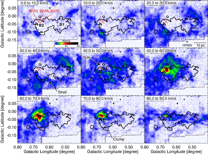
Figure 1: Velocity channel distributions of C¹⁸O($J$=2–1) toward the Sgr B region, including Sgr B1 and Sgr B2, obtained with APEX, overlaid with thick black contours outlining the 90 cm radio-continuum emission. The red circles indicate the positions of Sgr B2(N), (M), and (S), respectively. Known CO features (the Shell, the Hole, and the Clump) are labeled.

Figure 1 shows the velocity channel distribution of C¹⁸O($J$=2–1) toward the Sgr B region. Molecular clouds with velocities out of the figure are located in the foreground or in the so-called “expanding molecular ring” (Kaifu et al., 1972), and are not associated with Sgr B1 and Sgr B2 (see also Figure 4 of Vastel et al., 2002). The positions of the active star-forming regions (Sgr B1, Sgr B2) and star-forming cores (Sgr B2(N), Sgr B2(M), and Sgr B2(S)) are indicated in the top-left panel. The black contours indicate the boundaries of the active star-forming regions obtained from the 90 cm radio-continuum data (LaRosa et al., 2000). As seen in Figure 1, C¹⁸O($J$=2–1) traces the diffuse gas well, and it peaks at $V_{LSR}$ $\sim 60$ km s^-1 toward Sgr B2(M), meaning that there is no significant self-absorption, even toward Sgr B2(M). At $V_{LSR}$ = 20–40 km s^-1, 40–50 km s^-1, and 60–80 km s^-1, the Shell appears as a $\sim$30 pc cavity, the Hole is slightly north of Sgr B2, and the Clump is located near the star-forming cores, as proposed by Hasegawa et al. (1994). The figure shows that the Clump is obviously associated with the star-forming cores. This has already been reported in the literature (e.g., Tsuboi et al., 1999). The shapes of the Shell and the black contours agree well with each other. The filamentary clouds elongated in the direction of Galactic longitude in $V_{LSR}$ $\sim$80–90 km s^-1 are probably located in another arm (arm II; Sofue, 1995) or stream (Kruijssen et al., 2015).

4.2 Application of the CCC Identification Methodology

In this section, we use the identification methodology developed by Fukui et al. (2018a) and Enokiya et al. (2021a) to investigate the possibility of a CCC in the Sgr B region. As described in Section 2.2, we use the C¹⁸O($J$=2–1) line as the best tracer for the methodology in this region.

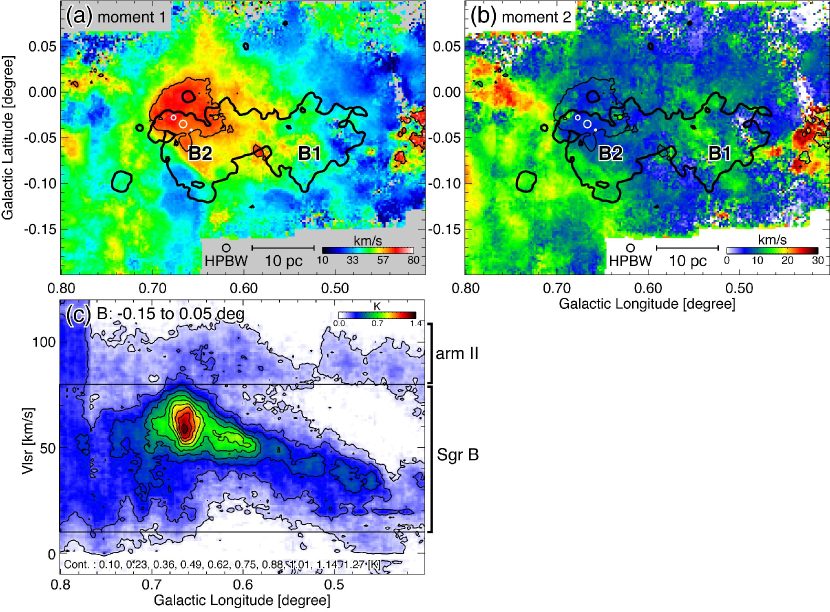
Figure 2: Panels (a) and (b): intensity-weighted first-moment and second-moment maps of C¹⁸O($J$=2–1) in 10 $\leq$ $V_{LSR}$ $\leq$ 80 km s^-1. The white circles indicate the positions of Sgr B2(N), (M), and (S). The thin and thick black contours indicate the boundaries of the first-moment = 60.0 km s^-1 and the radio-continuum emission at 90 cm, respectively. Panel (c): longitude–velocity diagram for C¹⁸O($J$=2–1) toward the Sgr B region. The black lines indicate the velocity range used for the moment calculations.

Following Enokiya et al. (2021a), we first define the velocity components in this region by analyzing the moments of C¹⁸O($J$=2–1). Figures 2(a) and 2(b) show the distributions of the intensity-weighted mean velocity and the standard deviation of the velocity, respectively. We used only voxels with at least a 5 $\sigma$ significance level for this analysis, in order to reduce noise fluctuations. Figure 2(c) shows a longitude-velocity diagram toward the Sgr B region. The associated clouds reported in previous works are seen as major bright features in 10 $\leq$ $V_{LSR}$$\leq$ 80 km s^-1, indicated by the black lines. We use this velocity range to calculate the moments. Figure 2(a) shows that redshifted features (from the interior to the thin black contour: $V_{LSR}$ $\geq$ 60 km s^-1) are seen toward the star-forming cores in Sgr B2. This component contains the Clump (Hasegawa et al., 1994). We hereafter call this velocity component the “60 km s^-1 component”. The exterior of the black contour shows velocity gradients ranging from yellow to blue in Figure 2a. We hereafter call this velocity feature the “40 km s^-1 component”. The eastern contact line of the 60 km s^-1 component has relatively larger line widths, colored light green (Figure 2(b)).

In accordance with Enokiya et al. (2021a), we determine $V_{\mathrm{center}}$ and $dV$, respectively, as the averages of velocity of the first and second moments in the given area, and we take the representative velocity range to be $V_{\mathrm{center}}$ $\pm$ $dV$. We use the interior and exterior of the thin black contour (first moment = 60.0 km s^-1) in Figure 2(a) as the 60 km s^-1 and 40 km s^-1 component areas, respectively. We have confirmed that the difference between these areas does not significantly change the results shown below. We list the representative velocity range, $V_{\mathrm{center}}$, and $dV$ for each velocity component in Table 1.

Table 1: Physical Parameters of the Velocity Components

Name	Representative velocity range	$V_{\mathrm{center}}$	$dV$	$N_{\mathrm{H_{2}}}$ (typical/peak)	Mass
	(km s-1)	(km s-1)	(km s-1)	($\times$1023 cm-2)	($\times$106 M⊙)
40 km s-1 component	29 – 53	41.6	12.2	$\sim$0.5 / 1.7	1.4
60 km s-1 component	53 – 74	63.8	10.4	$\sim$1 / 6.6	1.1

Note. — Column 1: names of the components, column 2: velocity ranges; column 3: peak velocities derived from the moment 1 map; column 4: velocity line widths derived from the moment 2 map; column 5: typical and peak molecular column densities toward each component; column 6: molecular masses.

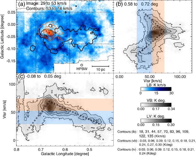
Figure 3: Panel (a): integrated intensity distributions of the 40 km s^-1 component (blue color) and 60 km s^-1 component (orange contours) in C¹⁸O($J$=2–1). Panels (b)and (c): velocity–latitude diagram and longitude–velocity diagram of C¹⁸O($J$=2–1) toward the Sgr B region. The velocity integration ranges for the 40 km s^-1 and 60 km s^-1 components are indicated by the transparent blue and orange belts, respectively.

Figures 3(a)–3(c) show the integrated intensity distributions, the velocity–latitude diagram, and the longitude–velocity diagram for the 40 km s^-1 and 60 km s^-1 components in C¹⁸O($J$=2–1). The two velocity components exhibit the typical signature of a CCC: a complementary distribution in space (Figure 3(a)). The star-forming cores, indicated as the red circles, are located at the intensity peak of the higher–column density cloud, the 60 km s^-1 component. Furthermore, there are rotated, V-shaped features in the position–velocity diagrams. All of these features are typical signatures of a CCC. We also investigated the SiO emissions and the line-intensity ratios between C¹⁸O($J$=2–1) and C¹⁸O($J$=1–0) (R${}_{2-1/1-0}^{18}$) toward this region (see the Appendix, Figures 9 and 10). From Figure 4 of Nishimura et al. (2015), the typical value of R${}_{2-1/1-0}^{18}$ and those in the star-forming regions in Orion are $\sim$0.5 and 1.0–1.2, respectively. In the Sgr B region, a typical value of R${}_{2-1/1-0}^{18}$ is $\sim$0.8; it is higher at the boundary of the Shell and the boundary of the Hole (1.0–1.6) and highest at the Clump (1.6–2.8). The SiO($J$=5–4) emissions are detected only in the areas where R${}_{2-1/1-0}^{18}$ is higher.

4.3 Physical Parameters of the Two Components

Here, we derive physical parameters, such as column densities and masses, for the 40 km s^-1 and 60 km s^-1 components, assuming local thermodynamic equilibrium (LTE). We assume that the excitation temperature is $T_{\mathrm{ex}}$ = 30 K, which is similar to the temperatures of previous studies (Hasegawa et al., 1994; Morris et al., 1983). Although the temperatures may vary with position or component, the differences in $T_{\mathrm{ex}}$ do not significantly affect the results.

First, we define the equivalent brightness temperature $J(T)$ as

$$J(T)=\frac{h\nu}{\mbox{$k_{\mathrm{B}}$}}~{}[~{}\exp(\frac{h\nu}{\mbox{$k_{\mathrm{B}}$}T-1})~{}]^{-1}.$$ (1)

where $h$, k_B, and $\nu$ are Planck’s constant, Boltzmann’s constant, and the frequency, respectively. A variation of the radiative transfer equation gives the optical depth $\tau_{\nu}$ as

$$\tau(v)=-\ln(~{}1~{}-~{}\frac{\mbox{$T_{\mathrm{obs}}$}}{J(\mbox{$T_{\mathrm{ex}}$})~{}-~{}J(\mbox{$T_{\mathrm{bg}}$})}~{}).$$ (2)

where $T_{\mathrm{obs}}$ and $T_{\mathrm{bg}}$ are the observed intensity on the $T_{\mathrm{mb}}$ scale and the temperature of the background (= 3 K), respectively. The column density $N$ of the molecules can be calculated as follows:

$$N=\sum_{V}~{}\tau(v)~{}\Delta v~{}\frac{3\mbox{$k_{\mathrm{B}}$}\mbox{$T_{\mathrm{ex}}$}}{4\pi^{3}\nu\mu^{2}}~{}\exp(\frac{h\nu J}{2\mbox{$k_{\mathrm{B}}$}\mbox{$T_{\mathrm{ex}}$}})~{}\frac{1}{1-\exp({-\frac{h\nu}{\mbox{$k_{\mathrm{B}}$}\mbox{$T_{\mathrm{ex}}$}}})},$$ (3)

where $V$, $\Delta v$, $\mu$, and $J$ are the velocity of the cloud, the velocity resolution of the data, the electric-dipole moment of the molecule, and the rotational transition level, respectively. Substituting $k_{\mathrm{B}}$ = 1.38 $\times~{}10^{-16}$ (erg/K), $T_{\mathrm{ex}}$ = 30 (K), $\nu$ = 2.196 $\times~{}10^{11}$ (Hz), $\mu$ = 1.10 $\times~{}10^{-19}$ (esu cm), $h$ = 6.63 $\times~{}10^{-27}$ (erg s), and $J$ = 1 into Equation (3) gives

$$\mbox{$N_{\mathrm{C^{18}O}}$}=1.518\times 10^{16}~{}\sum_{V}~{}\tau(v)~{}\Delta v.$$ (4)

The relation between $N_{\mathrm{C^{18}O}}$ and $N_{\mathrm{H_{2}}}$ was determined by Frerking et al. (1982) to be

$$\mbox{$N_{\mathrm{H_{2}}}$}=(\frac{\mbox{$N_{\mathrm{C^{18}O}}$}}{1.7\times 10^{14}}+1.3)\times 10^{21}.$$ (5)

Using Equations (4) and (5), we find the typical / peak column densities of the 40 km s^-1 and 60 km s^-1 components to be 0.5 / 1.7 $\times$ 10²⁴ and 1 / 6.6 $\times$ 10²³ cm^-2, respectively.

The molecular mass is determined from following equation:

$$M=\mbox{$\mu_{\mathrm{m}}$}\mbox{$m_{\mathrm{p}}$}\sum_{i}~{}[d^{2}\Omega\mbox{$N_{\mathrm{H_{2}}}$}_{,i}],$$ (6)

where $\mu_{\mathrm{m}}$, $m_{\mathrm{p}}$, $d$, $\Omega$ and $\mbox{$N_{\mathrm{H_{2}}}$}_{,i}$ are the mean molecular weight, proton mass, distance, solid angle subtended by a pixel, and column density of molecular hydrogen for the $i$th pixel, respectively. We assume a helium abundance of 20$\%$, which corresponds to $\mu_{\mathrm{m}}$ = 2.8. If we take $d$ = 8300 pc, the masses of the 40 km s^-1 and 60 km s^-1 components are $\sim$1.4 and $\sim$1.1 $\times$ 10⁶ M_⊙, respectively. These physical parameters are listed in Table 1.

4.4 Multiwavelength View of the Sgr B Region

Above, we have defined two velocity components (the 40 km s^-1 component and 60 km s^-1 component), and we have shown that a CCC model is applicable in this region. In this section, we present a multiwavelength view of the region and compare it with the results obtained in the previous section.

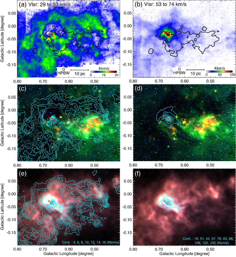
Figure 4: Panels (a) and (b): integrated intensity distributions of the 40 km s^-1 component and the 60 km s^-1 component in C¹⁸O($J$=2–1), obtained with APEX. The red circles indicate the positions of Sgr B2(N), (M), and (S), from north to south. The thick black contours indicate the outline of the radio-continuum emission at 90 cm. Panels (c) and (d): the cyan contours obtained from the distributions of C¹⁸O($J$=2–1) in Figures 4(a), and 4(b), respectively are superposed on a three-color composite image obtained with Spitzer. The red, green, and blue correspond to 24, 8, and 3.6 $\mu$m, respectively. Panels (e) and (f): the same contours of Figures 4(b), and 4(c), respectively, are superposed on a three-color composite image obtained with Herschel. Here, the red, green, and blue correspond 500, 350, and 250 $\mu$m, respectively.

Figure 4(a) shows the spatial distribution of the 40 km s^-1 component, overlaid with the black contours of the boundary of the star-forming region traced by the 90 cm radio-continuum emission. The representative velocity ranges defined in Section 4.2 are used as the integration ranges. Figures 4(c) and 4(e) are superpositions of contours of the contours of the 40 km s^-1 component on the MIR and FIR images obtained with Spitzer and Herschel, respectively. The FIR composite image shows only a single burgundy color. This likely indicates that the properties of the cold dust emitting the FIR are the same throughout this region, except for the white area, where the radiation is very strong and saturated. The cold dust is seen as dark clouds in the MIR, which means that a bright MIR source radiates from behind. The major radiative process in the MIR is irradiation with UV photons from high-mass stars, so the MIR is another indicator of star-forming activity, in addition to the radio-continuum. It is clear that the bright MIR regions coincide well, excluding the vicinity of the star-forming cores, with the radio-continuum boundary (the black contour in Figure 4(a)). Thus, the bright background sources are Sgr B1 and Sgr B2.

The distribution of the 40 km s^-1 component in the dense-gas tracer, C¹⁸O($J$=2–1), is very similar to that of the cold dust or the MIR dark clouds. These three therefore originate from the same object at different wavelengths, and they are located in front of Sgr B1 and Sgr B2. At the northwest edge of Sgr B1, the integrated intensity of C¹⁸O($J$=2–1) is enhanced and well delineate the boundary of the radio-continuum emission (Figure 4(a)); thus, the 40 km s^-1 component is likely interacting with Sgr B1. These are the dense clouds labeled “cloud d” and “cloud e” by Longmore et al. (2013).

Figure 4(b) also shows the spatial distribution of the 60 km s^-1 component in C¹⁸O($J$=2–1), overlaid with the black contours of the boundary of the star-forming region traced by the 90 cm radio-continuum emission. Figures 4(d) and 4(f) are similar superpositions of the contours of the 60 km s^-1 component on the MIR and FIR images obtained with Spitzer and Herschel, respectively. The 60 km s^-1 component coincides with the strong FIR peak and the star-forming cores in Sgr B2. This result clearly shows that the star-forming cores of Sgr B2 are still at a very young stage of cluster formation, and are deeply embedded in the high-density cloud with $N_{\mathrm{H_{2}}}$ $\geq$ 10²³ cm^-2, as already reported in ealier studies. The 60 km s^-1 component is also dark in the MIR image, although this region is very bright in the radio-continuum. Thus, the 60 km s^-1 component is located a bit closer to the Sun than Sgr B2. The darkness in the MIR image also indicates that Sgr B2 is a much younger system than Sgr B1.

4.5 Summary of Observational Insights

Here, we summarize the observational aspects of the Sgr B region and the results of our analyses.

1. Following Enokiya et al. (2021a), we identified two velocity features (the 40 km s^-1 and 60 km s^-1 components) associated with Sgr B1 and Sgr B2 by using moment maps of C¹⁸O($J$=2–1).

2. These two components clearly show all the signatures of a CCC proposed by Fukui et al. (2018a): the complementary spatial distribution between the two components, the V-shaped structure formed by the two colliding clouds in the position–velocity diagrams, and the coincidence between the location of the intensity peak of the denser component and the high-mass star-forming region. We also detected SiO emission, which accompanies CCCs in the GC (Enokiya et al., 2021a).

3. Using the LTE approximation, we estimated the physical parameters of the two velocity components with C¹⁸O($J$=2–1). The peak column densities and masses of the 40 km s^-1/60 km s^-1 components are $\sim$2 $\times$ 10²³ cm^-2 / $\sim$7 $\times$ 10²³ cm^-2, and 1.4 $\times$ 10⁶ M_⊙ / 1.1 $\times$ 10⁶ M_⊙, respectively.

4. By comparing the CO distributions and other wavelengths, we found that the 40 km s^-1 component, which is observed as an IR dark cloud, is located in front of Sgr B1 and Sgr B2. The 60 km s^-1 component is a high-density dust clump, with $N_{\mathrm{H_{2}}}$ $\geq$ 10²³ cm^-2, which includes star-forming cores. It is at a very young stage of cluster formation, and is located in front of Sgr B2.

5 Discussion

In the previous Section, we applied the CCC identification methodology to the Sgr B region and found clear signatures of a CCC. In this section, we investigate further observational evidence for a CCC and discuss the CCC scenario, including star-forming activities.

5.1 Comparison with Numerical Simulations

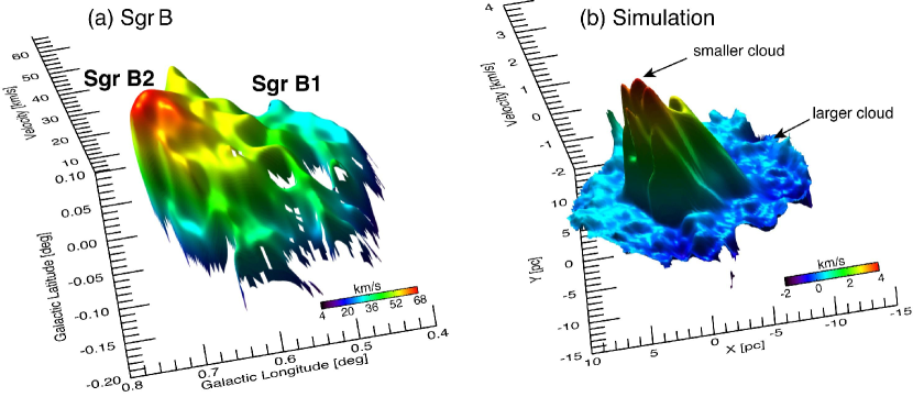
Figure 5: Panel (a): longitude-latitude-velocity surface plot of the Sgr B region in C¹⁸O($J$=2–1). Panel (b): ppv surface plot of a numerical simulation of a CCC performed by Takahira et al. (2014) and Haworth et al. (2015).

Figures 5(a) and 5(b), respectively, show a lngitude-latitude-velocity surface plot of C¹⁸O($J$=2–1) in the Sgr B region and a position-position-velocity (ppv) surface plot in the ¹²CO($J$=1–0) synthetic observational data obtained by Haworth et al. (2015) (for a head-on collision with a relative velocity of 10 km s^-1, observed from the angle of the relative motion). The color in Figure 5(a) corresponds to velocity. Both ppv plots show similar, cone-shaped structures. Henshaw et al. (2016) found a similar structure by using HNCO data obtained with the Mopra telescope (Jones et al., 2012). Note that these surface density plots were produced by velocities derived from the first moment (intensity-weighted mean velocity), and hence the velocity of the smaller cloud in the plot reflects the velocities of both the smaller and larger clouds, and does not directly present its original velocity. Thus, the quantitative comparison between Figure 5(a) and 5(b) does not make sense.

The conical structures seen in Figure 5 typically result from a collisional interaction between two clouds, due to the exchange of the clouds’ momenta, which is observed as the V shape in the position–velocity diagram (See Section 2.1). This structure is easily weakened by projection effects (see Fukui et al., 2018a, for details). The observation shows a clear conical structure, but the apex is shifted slightly from the center, in the direction of positive Galactic longitude, suggesting that the collision may not be head-on and that the 60 km s^-1 component has a relative velocity toward positive Galactic longitudes (see Fukui et al., 2018a, for details).

The part of the larger cloud that surrounds the cone shape, but that does not participate in any collisional interactions, preserves the larger cloud’s original velocity structures, as illustrated by the light and dark blue in Figure 5(b). In the observational data, the velocity gradient of the cone extends from the eastern boundary of Sgr B2 to the western boundary of Sgr B1. Thus, if we adopt the CCC model, a comprehensive CCC probably occurred between the two clouds, as shown in light blue and red in Figure 5(a). These two clouds correspond to the Shell and the Clump. Sgr B1 is located in the interior of the Shell, and thus it is possible that not only Sgr B2, but also Sgr B1, were triggered by the CCC. Larger velocity widths are observed at the collisional interface (that is, at the base of the cone structure in the synthetic observations), and the enhanced line widths and SiO emissions detected along the inner boundary of the Shell lend support to a comprehensive collision at the 30 pc scale.

Figure 4(c) shows that the 40 km s^-1 component, which appears dark, intercepts the MIR emission from the background source, Sgr B1. In spite of this, the boundary of the MIR emission from Sgr B1 coincides with the optically thin radio-continuum emission, which is not intercepted by the foreground cloud of the 40 km s^-1 component (see Figure 4(a)). This means that the star-forming activities of Sgr B1 only spread toward the region where the CO intensity of the 40 km s^-1 component is depressed. This is clear evidence that a past collision at the position of Sgr B1 hollowed out the 40 km s^-1 component and created the hole, and that the collision triggered high-mass star formation in Sgr B1. Conversely, if we abandon the CCC model, the coincidence between the CO and radio-continuum toward Sgr B1 is rather unnatural.

5.2 CCC Scenario

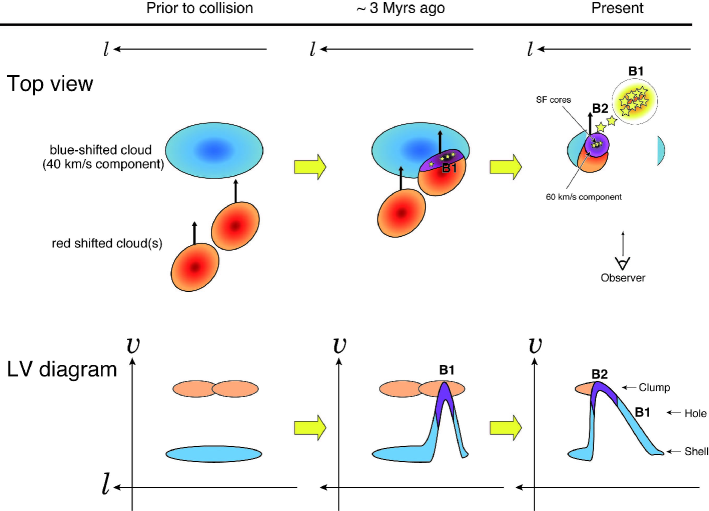
Figure 6: Upper panel: schematic image of the time evolution of the CCC in the Sgr B region (top view). Lower panel: schematic image of the time evolution of the longitude–velocity diagram.

From the above discussion, we here propose the following plausible collision scenario: two redshifted clouds—or one large redshifted cloud with two density peaks—approached a blueshifted cloud (the leftmost panel of Figure 6). About 3 Myr ago, the two velocity features started to collide at the position of Sgr B1, and formed Sgr B1 first (the middle panel of Figure 6). The region involved in this collision then extended from west to east (from Sgr B1 to Sgr B2). A recent collision at the positions of Sgr B2(N), (M), and (S) triggered star-forming activities there (the rightmost panel of Figure 6). The blueshifted cloud is likely to be the 40 km s^-1 component. If we assume the age of Sgr B1 to be 3 Myr, then, by dividing the distance between Sgr B2 and Sgr B1 by the age, we obtain the speed at which the collision spread along the Galactic longitude as 30 pc / 3 Myr = 10 km s^-1.

We suggest two possible candidates for the redshifted cloud(s). One possibility is that the clouds are located in arm II at $V_{LSR}$ $\sim$90 km s^-1, as shown in Figures 1 and 2(c). These figures show that the 60 km s^-1 component connects to arm II in space and velocity. In this case, the velocity difference of $\sim$30 km s^-1 between the 60 km s^-1 component and arm II can be explained by the exchange of momenta between the 40 km s^-1 component and arm II (90 km s^-1). The other possibility is a cloud with an initial velocity of $\sim$60 km s^-1. If this cloud had a very high-density, compared to that of the 40 km s^-1 component, the cloud might maintain its initial velocity even after the collision. However, there is so far no clear evidence for the existence of clouds with 60 km s^-1 in this direction, and furthermore, the 60 km s^-1 component has apparently extended gas to the higher velocity (see e.g., Figure 3(b)), then the first case might be more plausible.

According to Fukui et al. (2018a) two velocity components are not always observable in a CCC, due to projection effects and so on. Fukui et al. (2018b) present a case of a CCC with a single-velocity component in the star cluster GM24. Therefore, even though the conical structure in the ppv plot consists of a single-peak velocity profile, this model is still possible.

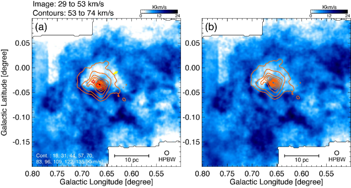
Figure 7: Panel (a): close-up view of integrated intensity distribution of the 40 km s^-1 component (blue color) and the 60 km s^-1 component (orange contours). The red circles indicate the positions of Sgr B2(N), (M), and (S). Panel (b): the same as Figure 7(a), but the contours are displaced 4 pixels (1.16 pc) to the west and 2 pixel (0.58 pc) to the north. The length and the direction of the displacement is indicated by the yellow arrow in Figure 7(a).

Figure 7(a) shows distributions of the 40 km s^-1 component (blue contours) and the 60 km s^-1 component (orange contours). The distributions of the hole in the 40 km s^-1 component and the 60 km s^-1 component display a slight displacement. Following Enokiya et al. (2021a), and by using an algorithm developed by Fujita et al. (2021), we estimate the displacement to be $\sim$1.3 pc to the northwest, which maximizes the complementarity between the two components. The yellow arrow in Figure 7(a) indicates the derived displacement vector. Figure 7(b), which shows the contours displaced by that arrow overlaid on the 40 km s^-1 component, exhibits perfect coincidence between the two components. Three active star-forming cores are located at the center of the 60 km s^-1 component. If we assume that the LOS relative velocity and the relative velocity in the direction of Galactic longitude are same, then by dividing the displacement by the relative velocity, we estimate the duration time of the collision at the star-forming cores to be 1 pc/30 km s^-1 $\simeq$ 4 $\times$ 10⁴ yr. This value is comparable to the typical age of hypercompact Hii regions (10³–10⁴ yr, e.g., Qin et al., 2008). From numerical MHD simulations, Fukui et al. (2021) reported that molecular flows colliding at a relative velocity of 20 km s^-1 and with densities of 1000 cm^-3 generate massive clumps at the collision interface, with mass accretion rates larger than 10^-4 M_⊙ yr^-1. Since the 60 km s^-1 component is denser than their simulations, a CCC is a viable process for creating the star-forming cores.

5.3 Origin of the Large Velocity Difference between the Two Clouds

The driving force responsible for producing the large relative velocity of a few tens of km s^-1 between two massive clouds is still unclear, but we propose two possibilities. One is a bar-potential-driven model. As Binney et al. (1991) originally proposed, two families of x1 and x2 orbits can be produced in the central 1 kpc of a galaxy under certain bar-potential conditions. The probability of a CCC increases at the intersections of these orbits (or arms). According to the x1–x2 orbits dynamical model, as in Binney et al. (1991), Bally et al. (2010), and Molinari et al. (2011), the Sgr B region is located at one of the intersections.

Based on hydrodynamic simulations, Sormani et al. (2019) discussed the origins of extended velocity features (EVFs), and suggested that EVFs are consequently obtained as results from two types of cloud collisions, overshot type or connection type, accelerated by the bar potential. The overshot type requires an interloper, which is overshoot from the dust lane. The redshifted clouds likely belong to arm II (see Section 5.2), and have not been overshoot; thus, the other cloud—i.e., the blueshifted cloud, or, in other words, the 40 km s^-1 component—should be overshot from a dust lane resulting from bar-potential acceleration, if this model is true. Although the mass and size of the overshoot cloud is quite large (see Table1), and thus it is apparently unnatural, it still remains a possible scenario. If the Sgr B region is a connection type EVF, it needs to be a connecting point for at least two streams. As discussed at the beginning of this section, this scenario is also possible.

Another possibility is a magnetically driven model. The GC has strong magnetic fields at least 50 $\mu$G (Crocker et al., 2010), and such conditions can easily excite Alfvén velocities of the order of a few tens of km s^-1 (see Suzuki et al., 2015). Some authors have also reported observational evidence of loop-like gas streams perpendicular to the Galactic plane produced by magnetic buoyancy (Fukui et al., 2006; Enokiya et al., 2014). The probability of a CCC increases at the footpoints of these loops. Enokiya et al. (2021a) discovered an enhancement in the probability of a CCC at the footpoints of the loops. They suggested that the enhancement is caused by rear end collisions originated from the stagnation of the flow at the footpoints. According to the open-orbit dynamical model, the orbit has warps in $z$-direction. Although this warp has so far not been clearly explained, if we assume that the warp is reflecting the shape of toroidal magnetic field line, the Sgr B region is located at the foot point of the loop (i. e., the base of the warp). Thus, the collision at the Sgr B region can be interpreted as a rear end collision resulting from the gravitationally accelerated cloud sliding down along the loop.

5.4 The Star Formation Triggered by the CCC Event

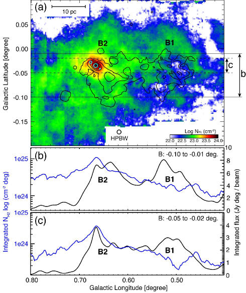
Figure 8: Panel (a): H₂ column-density map of the molecular gas associated with the Sgr B region estimated from the C¹⁸O($J$=2–1) emission in 20 km s^-1 $\leq$ $V_{LSR}$ $\leq$ 90 km s^-1. The contours show the distribution of the radio-continuum emission at 90 cm. The cyan circles indicate the positions of Sgr B2(N), (M), and (S). The integration latitude ranges for Figures 8(b) and 8(c) are indicated by the black lines and dashed black lines, respectively. Panel (b): the integrated column density (blue) and integrated 90 cm flux (black) plots toward the star-forming regions in the Sgr B region. Panel (c): the same plots for the limited latitude range focused on the Sgr B2 star-forming cores.

The image and contours in Figure 8(a) show the distributions of the column densities ($N_{\mathrm{H_{2}}}$) derived by using the LTE approximation and the radio-continuum emission, respectively. We adopted $T_{\mathrm{ex}}$ = 30 K and the velocity range 20 $\leq$ $V_{LSR}$ $\leq$ 90 km s^-1 for the calculation. Figure 8(a) clearly shows that the column density is typically $\sim$10²³ cm^-2 and increases up to $\sim$10²⁴ cm^-2 toward the star-forming cores, and it decreases to less than $\sim$10²² cm^-2 toward Sgr B1. We assume here that the radio-continuum emission is optically thin, in which case it is a good tracer of star formation activity. Figures 8(a) shows that the correlations between gas and star-formation activity get better/worse toward Sgr B2/Sgr B1.

The plots of the integrated $N_{\mathrm{H_{2}}}$ and radio-continuum flux versus the Galactic longitude shown in Figures 8(b) and 8(c) delineate the above picture more quantitatively. The integrated latitude ranges of Figure 8(b) and 8(c) correspond to the two star-forming regions and the star-forming cores, respectively. Figure 8(b) shows that the star-forming activities in Sgr B1 and Sgr B2 are fairly comparable, although the mass of the molecular gas concentrated in Sgr B2 is one order of magnitude higher than in Sgr B1. This may mean that 90$\%$ of the molecular gas in Sgr B1 has been consumed to form stars or has been dissipated by ionization or the CCC. As discussed in Section 5.1, the shape of the cavity in the 40 km s^-1 component and Sgr B1 are very similar, although they have slightly different LOS distances. Therefore, the collision may have hollowed out the 40 km s^-1 component, creating the cavity and triggering high-mass stars, thus dissipating the natal cloud. Figure 8c shows that $\sim$50$\%$ of the star-forming activity and the molecular gas in Sgr B2 are contained in a small volume. On the other hand, the molecular gas in Sgr B1 is significantly decreased. Again, this depression is likely caused by the collision and ionization.

5.5 Position of the Sgr B Region among Other CCC Regions

Enokiya et al. (2021a) collected all the literature reporting the signatures of CCCs, and they carried out a statistical analysis of the data. For more than 50 Galactic objects, they found correlations between the number of O- and early B-type stars and the peak column densities of the colliding clouds, as well as between the relative velocities and peak column densities of the colliding clouds (see Figure 9 of Enokiya et al., 2021a). The CCC in the Sgr B region shows the following relative velocity, peak column density, and number of high-mass stars (candidates): 22 km s^-1, $\sim$10²⁴, and a few hundreds, respectively, in the star forming cores. These physical parameters mostly satisfy the correlations found by Enokiya et al. (2021a) for the most massive cases.

The correlation plots indicate that only a CCC with a lower column density triggers the formation of a normal star cluster, that a moderate column density triggers a superstar cluster, and that a high column density may trigger a starburst. The threshold column densities for triggering a normal cluster, a superstar cluster, and a starburst are $\sim$10^21.5, $\sim$10²³, and $\sim$10²⁴ cm^-2, respectively. Some authors have suggested that a collision between two large-scale Hi flows can trigger a massive cluster containing M_∗ of a few hundred thousands M_⊙, such as R136 in the Large Magellanic Cloud (Fukui et al., 2017; Tachihara et al., 2018). Detailed molecular observations of the star-forming cores in Sgr B2 with ALMA may reveal the CCC star-forming process at a very young stage, and link the triggering mechanism with the active star formation seen in the external galaxies.

6 Summary

We have used a recently developed CCC identification methodology to investigate the possibility of a CCC in the Sgr B region, by using datasets at various wavelengths and fully sampled molecular-line data. Our major findings are summarized as follows.

1. We identified two CO components, with velocities of $\sim$42 (the 40 km s^-1 component) and $\sim$64 km s^-1 (the 60 km s^-1 component) by using C¹⁸O($J$=2–1) as the optically thin, dense-gas tracer. These velocity components form a cone-like structure covering both Sgr B1 and Sgr B2 in the ppv plot.

2. From comparisons with other wavelengths, we identified the locations of the velocity components and the star-forming regions in the Sgr B region as follows: Sgr B1 and Sgr B2 are located farthest from the Sun, while the 40 km s^-1 component is nearest, and intercepts the light from Sgr B1 and Sgr B2. The star-forming cores in Sgr B2—namely Sgr B2(N), (M), and (S), accompanied by the 60 km s^-1 component—are located nearer to the remaining region of Sgr B2. According to previous work, Sgr B2 is likely to be located nearer to the Sun than Sgr B1. Although the LOS distances to Sgr B1 and the 40 km s^-1 component are likely to be slightly different, the distributions of these two regions show an interaction between them.

3. Two clouds satisfy all the signatures of a CCC, as suggested by Fukui et al. (2018a). If we apply the CCC model, Sgr B1 and Sgr B2 are explained as results of contiguous collisions between the 40 km s^-1 and redshifted clouds. One of the cores of the redshifted cloud, with a column density of 10^23-24 cm^-2, collided first and formed Sgr B1 a few Myr ago, while a very recent collision of another core of the redshifted cloud a few $\times$ 10⁴ yr ago triggered active star formation in the star-forming cores in Sgr B2, which include a few hundred high-mass stars. The candidates for the redshifted cloud are either a cloud with a velocity of $\sim$60 km s^-1 or the so-called arm II.

4. The CCC in the Sgr B region satisfies the correlation among the relative velocity, peak column density, and the number of O- and early B-type stars found in Enokiya et al. (2021a) in the most active star formation case.

Although we do not have clear evidence for this, the mechanism responsible for driving the large relative velocity of the clouds may either be an encounter between arms or streams, or else a magnetic instability, such as the Parker instability. Higher-resolution observations will be required in order to determine the detailed mechanism responsible for triggering star formation in Sgr B2.

Appendix A Appendix information

Here we show the distributions of the shocked gas (Figure 9) and the relative excitation states (Figure 10) toward the Sgr B1 and Sgr B2 regions. Figures 9 and 10 show the velocity channel distributions of SiO($J$=5–4) and R${}_{2-1/1-0}^{18}$, respectively.

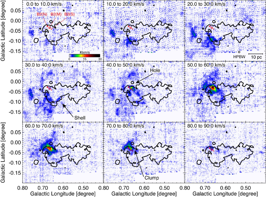
Figure 9: Velocity channel distributions of SiO($J$=5–4) toward the Sgr B region, obtained with APEX, overlaid with the thick black contours of the 90 cm radio-continuum emission. The red circles indicate the positions of Sgr B2(N), (M), and (S).

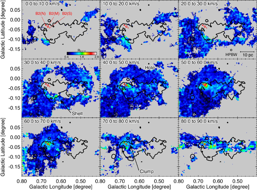
Figure 10: Velocity channel distributions of the intensity ratios of C¹⁸O($J$=2–1) and C¹⁸O($J$=1–0) toward the Sgr B region, overlaid with the thick black contours of the 90 cm radio-continuum emission. The red circles indicate the positions of Sgr B2(N), (M), and (S).

References

- Bally et al. (2010) Bally, J., Aguirre, J., Battersby, C., et al. 2010, ApJ, 721, 137
- Barnes et al. (2017) Barnes, A. T., Longmore, S. N., Battersby, C., et al. 2017, MNRAS, 469, 2263
- Belloche et al. (2013) Belloche, A., Müller, H. S. P., Menten, K. M., Schilke, P., & Comito, C. 2013, A&A, 559, A47
- Benson & Johnston (1984) Benson, J. M., & Johnston, K. J. 1984, ApJ, 277, 181
- Binney et al. (1991) Binney, J., Gerhard, O. E., Stark, A. A., Bally, J., & Uchida, K. I. 1991, MNRAS, 252, 210
- Braiding et al. (2018) Braiding, C., Wong, G. F., Maxted, N. I., et al. 2018, PASA, 35, e029
- Crocker et al. (2010) Crocker, R. M., Jones, D. I., Melia, F., Ott, J., & Protheroe, R. J. 2010, Nature, 463, 65
- Enokiya & Fukui (2021) Enokiya, R., & Fukui, Y. 2021, in Astronomical Society of the Pacific Conference Series, Vol. 528, New Horizons in Galactic Center Astronomy and Beyond, ed. M. Tsuboi & T. Oka, 279
- Enokiya et al. (2021a) Enokiya, R., Torii, K., & Fukui, Y. 2021a, PASJ, 73, S75
- Enokiya et al. (2014) Enokiya, R., Torii, K., Schultheis, M., et al. 2014, ApJ, 780, 72
- Enokiya et al. (2018) Enokiya, R., Sano, H., Hayashi, K., et al. 2018, PASJ, 70, S49
- Enokiya et al. (2021b) Enokiya, R., Ohama, A., Yamada, R., et al. 2021b, PASJ, 73, S256
- Fazio et al. (2004) Fazio, G. G., Hora, J. L., Allen, L. E., et al. 2004, ApJS, 154, 10
- Frerking et al. (1982) Frerking, M. A., Langer, W. D., & Wilson, R. W. 1982, ApJ, 262, 590
- Fukui et al. (2021) Fukui, Y., Habe, A., Inoue, T., Enokiya, R., & Tachihara, K. 2021, PASJ, 73, S1
- Fukui et al. (2017) Fukui, Y., Tsuge, K., Sano, H., et al. 2017, PASJ, 69, L5
- Fukui et al. (2006) Fukui, Y., Yamamoto, H., Fujishita, M., et al. 2006, Science, 314, 106
- Fukui et al. (2018a) Fukui, Y., Torii, K., Hattori, Y., et al. 2018a, ApJ, 859, 166
- Fukui et al. (2018b) Fukui, Y., Kohno, M., Yokoyama, K., et al. 2018b, PASJ, 70, S44
- Fukui et al. (2018c) Fukui, Y., Ohama, A., Kohno, M., et al. 2018c, PASJ, 70, S46
- Fux (1999) Fux, R. 1999, A&A, 345, 787
- Gaume et al. (1995) Gaume, R. A., Claussen, M. J., de Pree, C. G., Goss, W. M., & Mehringer, D. M. 1995, ApJ, 449, 663
- Ginsburg et al. (2016) Ginsburg, A., Henkel, C., Ao, Y., et al. 2016, A&A, 586, A50
- Ginsburg et al. (2018) Ginsburg, A., Bally, J., Barnes, A., et al. 2018, ApJ, 853, 171
- Goldsmith et al. (1987) Goldsmith, P. F., Snell, R. L., & Lis, D. C. 1987, ApJ, 313, L5
- Griffin et al. (2010) Griffin, M. J., Abergel, A., Abreu, A., et al. 2010, A&A, 518, L3
- Habe & Ohta (1992) Habe, A., & Ohta, K. 1992, PASJ, 44, 203
- Hasegawa et al. (2008) Hasegawa, T., Arai, T., Yamaguchi, N., & Sato, F. 2008, Ap&SS, 313, 91
- Hasegawa et al. (1994) Hasegawa, T., Sato, F., Whiteoak, J. B., & Miyawaki, R. 1994, ApJ, 429, L77
- Haworth et al. (2015) Haworth, T. J., Tasker, E. J., Fukui, Y., et al. 2015, MNRAS, 450, 10
- Hayashi et al. (2018) Hayashi, K., Sano, H., Enokiya, R., et al. 2018, PASJ, 70, S48
- Henshaw et al. (2016) Henshaw, J. D., Longmore, S. N., Kruijssen, J. M. D., et al. 2016, MNRAS, 457, 2675
- Hu et al. (2021) Hu, Y., Lazarian, A., & Wang, Q. D. 2021, arXiv e-prints, arXiv:2105.03605
- Inoue & Fukui (2013) Inoue, T., & Fukui, Y. 2013, ApJ, 774, L31
- Inoue et al. (2018) Inoue, T., Hennebelle, P., Fukui, Y., et al. 2018, PASJ, 70, S53
- Jones et al. (2012) Jones, P. A., Burton, M. G., Cunningham, M. R., et al. 2012, MNRAS, 419, 2961
- Kaifu et al. (1972) Kaifu, N., Kato, T., & Iguchi, T. 1972, Nature Physical Science, 238, 105
- Kauffmann (2016) Kauffmann, J. 2016, in From Interstellar Clouds to Star-Forming Galaxies: Universal Processes, ed. P. Jablonka, P. André, & F. van der Tak, Vol. 315, 163–166
- Kohno et al. (2018) Kohno, M., Torii, K., Tachihara, K., et al. 2018, PASJ, 70, S50
- Kruijssen et al. (2015) Kruijssen, J. M. D., Dale, J. E., & Longmore, S. N. 2015, MNRAS, 447, 1059
- Kruijssen et al. (2019) Kruijssen, J. M. D., Dale, J. E., Longmore, S. N., et al. 2019, MNRAS, 484, 5734
- LaRosa et al. (2000) LaRosa, T. N., Kassim, N. E., Lazio, T. J. W., & Hyman, S. D. 2000, AJ, 119, 207
- Lis & Goldsmith (1989) Lis, D. C., & Goldsmith, P. F. 1989, ApJ, 337, 704
- Longmore et al. (2013) Longmore, S. N., Kruijssen, J. M. D., Bally, J., et al. 2013, MNRAS, 433, L15
- Martín-Pintado et al. (1997) Martín-Pintado, J., de Vicente, P., Fuente, A., & Planesas, P. 1997, ApJ, 482, L45
- McGrath et al. (2004) McGrath, E. J., Goss, W. M., & De Pree, C. G. 2004, ApJS, 155, 577
- Mehringer et al. (1993) Mehringer, D. M., Palmer, P., & Goss, W. M. 1993, ApJ, 402, L69
- Mehringer et al. (1992) Mehringer, D. M., Yusef-Zadeh, F., Palmer, P., & Goss, W. M. 1992, ApJ, 401, 168
- Molinari et al. (2011) Molinari, S., Bally, J., Noriega-Crespo, A., et al. 2011, ApJ, 735, L33
- Morris et al. (1983) Morris, M., Polish, N., Zuckerman, B., & Kaifu, N. 1983, AJ, 88, 1228
- Morris & Serabyn (1996) Morris, M., & Serabyn, E. 1996, ARA&A, 34, 645
- Nishimura et al. (2015) Nishimura, A., Tokuda, K., Kimura, K., et al. 2015, ApJS, 216, 18
- Nishimura et al. (2018) Nishimura, A., Minamidani, T., Umemoto, T., et al. 2018, PASJ, 70, S42
- Ohama et al. (2018) Ohama, A., Kohno, M., Hasegawa, K., et al. 2018, PASJ, 70, S45
- Oka et al. (1998) Oka, T., Hasegawa, T., Sato, F., Tsuboi, M., & Miyazaki, A. 1998, ApJS, 118, 455
- Pilbratt et al. (2010) Pilbratt, G. L., Riedinger, J. R., Passvogel, T., et al. 2010, A&A, 518, L1
- Portail et al. (2017) Portail, M., Gerhard, O., Wegg, C., & Ness, M. 2017, MNRAS, 465, 1621
- Qin et al. (2008) Qin, S.-L., Huang, M., Wu, Y., Xue, R., & Chen, S. 2008, ApJ, 686, L21
- Rieke et al. (2004) Rieke, G. H., Young, E. T., Engelbracht, C. W., et al. 2004, ApJS, 154, 25
- Rodríguez-Fernández (2011) Rodríguez-Fernández, N. J. 2011, Memorie della Societa Astronomica Italiana Supplementi, 18, 195
- Sanders et al. (2019) Sanders, J. L., Smith, L., & Evans, N. W. 2019, MNRAS, 488, 4552
- Sano et al. (2018) Sano, H., Enokiya, R., Hayashi, K., et al. 2018, PASJ, 70, S43
- Sato et al. (2000) Sato, F., Hasegawa, T., Whiteoak, J. B., & Miyawaki, R. 2000, ApJ, 535, 857
- Simpson et al. (2018) Simpson, J. P., Colgan, S. W. J., Cotera, A. S., Kaufman, M. J., & Stolovy, S. R. 2018, ApJ, 867, L13
- Sofue (1990) Sofue, Y. 1990, PASJ, 42, 827
- Sofue (1995) —. 1995, PASJ, 47, 527
- Sormani et al. (2015) Sormani, M. C., Binney, J., & Magorrian, J. 2015, MNRAS, 454, 1818
- Sormani et al. (2020) Sormani, M. C., Tress, R. G., Glover, S. C. O., et al. 2020, MNRAS, 497, 5024
- Sormani et al. (2018) Sormani, M. C., Treß, R. G., Ridley, M., et al. 2018, MNRAS, 475, 2383
- Sormani et al. (2019) Sormani, M. C., Treß, R. G., Glover, S. C. O., et al. 2019, MNRAS, 488, 4663
- Suzuki et al. (2015) Suzuki, T. K., Fukui, Y., Torii, K., Machida, M., & Matsumoto, R. 2015, MNRAS, 454, 3049
- Tachihara et al. (2018) Tachihara, K., Gratier, P., Sano, H., et al. 2018, PASJ, 70, S52
- Takahira et al. (2014) Takahira, K., Tasker, E. J., & Habe, A. 2014, ApJ, 792, 63
- Tokuyama et al. (2019) Tokuyama, S., Oka, T., Takekawa, S., et al. 2019, PASJ, 71, S19
- Torii et al. (2018) Torii, K., Fujita, S., Matsuo, M., et al. 2018, PASJ, 70, S51
- Tsuboi et al. (1999) Tsuboi, M., Handa, T., & Ukita, N. 1999, ApJS, 120, 1
- Umemoto et al. (2017) Umemoto, T., Minamidani, T., Kuno, N., et al. 2017, PASJ, 69, 78
- Vastel et al. (2002) Vastel, C., Polehampton, E. T., Baluteau, J. P., et al. 2002, ApJ, 581, 315
- Wegg & Gerhard (2013) Wegg, C., & Gerhard, O. 2013, MNRAS, 435, 1874
- Young et al. (1986) Young, J. S., Kenney, J. D., Tacconi, L., et al. 1986, ApJ, 311, L17
- Yusef-Zadeh et al. (2004) Yusef-Zadeh, F., Hewitt, J. W., & Cotton, W. 2004, ApJS, 155, 421