Photogalvanic transport in fluctuating Ising superconductors

Abstract

In a two-dimensional noncentrosymmetric Ising superconductor in the fluctuating regime under the action of a uniform external electromagnetic field there emerge two contributions to the photogalvanic effect due to the trigonal warping of the valleys. The first contribution stems from the current of the electron gas in its normal state, while the second contribution is of Aslamazov-Larkin nature: it originates from the presence of fluctuating Cooper pairs when the ambient temperature approaches (from above) the temperature of superconducting transition in the sample. The way to lift the valley degeneracy is the application of a weak out-of-plane external magnetic field producing a Zeeman effect. The Boltzmann equations approach for the electron gas in the normal state and the time-dependent Ginzburg-Landau equations for the fluctuating Cooper pairs allow for the study of the photogalvanic current in two-dimensional transition metal dichalcogenide Ising superconductors.

I Introduction

In two-dimensional (2D) materials, photoinduced transport phenomena, which are second-order with respect to external electromagnetic (EM) field, are in the focus of state-of-the-art research [1]. The majority of these effects fall into two categories. The first one includes the rectification effects to occur under an external uniform alternating EM illumination, which produces stationary uniform electric currents in the system. The second category encompasses all the effects characterised by the system response at doubled field frequency, thus describing the second-harmonic generation phenomena.

The second-order transport phenomena are usually sensitive to the polarization of the EM field and the symmetry of the system under study, namely, the time-reversal symmetry and the spatial inversion symmetry. The phenomenological relation between the photoinduced rectified electric current and the amplitude of external EM field reads $j_{\alpha}=\zeta_{\alpha\beta\gamma}E_{\beta}E^{*}_{\gamma}$, where $\zeta_{\alpha\beta\gamma}$ is the third-order tensor acquiring non-zero components in non-centrosymmetric materials. In non-gyrotropic semiconductor materials, the (rectified) photoinduced electric current occurs as a second-order response to linearly polarized external EM wave. This constitutes the photogalvanic effect (PGE). This effect does not directly relate to either light pressure, the photon-drag phenomena, or non-uniformity of either the sample or light field intensity, like the photoinduced Dember effect. Instead, the microscopic origin of the conventional PGE lies in the asymmetry of the interaction potential or the crystal-induced Bloch wave function [2, 3, 4].

In modern Wan-der-Waals structures based on 2D monolayers of transition-metal dichalcogenides (TMDs) [5, 6], the PGE current may arise due to specific band structure of the material possessing two time-reversal-coupled valleys in the Brillouin zone. A typical example of these materials is molybdenum disulfide, MoS₂. It possesses the D_3h point group, and the presence of the $C_{3}$ axis results in the emergence of a trigonal warping of the electron dispersion in each valley reflecting the noncentrsymmetricity of the crystal structure. The theoretical analysis shows that the PGE current arises here in each valley (involving electrons residing in both the valleys), and these currents have different signs in different valleys. As a result, net PGE current self-compensates and vanishes. A nonzero net current may only occur if the time-reversal symmetry is broken due to, e.g., the presence of external magnetic field or illumination of the sample by a circularly-polarized EM field causing interband transitions [7, 8, 9].

Furthermore, a resent discovery of the superconducting (SC) transition in TMDs [10, 11, 12] stimulated additional interest to the study of transport phenomena in 2D Dirac materials exposed to external EM fields at lower temperatures [13, 14, 15]. In the intermediate range of temperatures lying in between the normal and SC state of the electron gas, when $0<T-T_{c}\ll T_{c}$ (where $T_{c}$ is a SC critical temperature), the order parameter starts to experience fluctuations [16, 17, 18]. Moreover, large spin-orbit coupling in TMDs results in strong out-of-plane electron spin polarization and large in-plane critical magnetic fields beyond the Pauli limit. Thus, all the ingredients of an Ising superconductor possessing unique physical properties are available. When the time-reversal symmetry breaks by a weak magnetic field due to the Zeeman effect, and given the absence of spatial reversal symmetry, TMDs might demonstrate pronounced nonreciprocal response in the regime of SC fluctuations [11, 12, 19, 20, 21, 22].

The goal of this work is to develop a microscopic theory of a linear PGE effect in fluctuating Ising superconductors exposed to linearly-polarized EM field. The time-reversal symmetry here is waved due to the presence of a weak Zeeman field pointed across the monolayer [23, 24]. Trigonal warping of the valleys $K$ and $K^{\prime}$ characteristic of MoS₂ serves as a microscopic mechanism of the effect. Within the D_3h point symmetry group, the third-order conductivity (or transport coefficient) tensor possesses only one nonzero component. Thus, phenomenologically, the PGE current can be expressed as $j_{x}=\zeta(|E_{x}|^{2}-|E_{y}|^{2}),\,\,j_{y}=-\zeta(E_{x}E^{*}_{y}+E_{x}^{*}E_{y})$. Therefore, the main task comes down to the calculation of the coefficient $\zeta$ and analyzing its behavior for various EM field frequencies and temperatures in the vicinity of $T_{c}$, taking into account the contribution of normal electrons and the corrections arising from the SC order parameter fluctuations.

II Effective electron dispersion in conduction band

The superconducting transition in MoS₂ monolayer occurs at electron densities exceeding $10^{14}$ cm^-2 [10]. At such high densities, the Fermi level lies deeply in the conduction band. Thus, it is feasible to use a simplified electron energy dispersion. Then, according to the two-band model, the Hamiltonian reads (in $\hbar=k_{B}=1$ units)

$$H=\frac{\Delta}{2}\sigma_{z}+v(\eta p_{x}\sigma_{x}+p_{y}\sigma_{y})+\left(\begin{array}[]{cc}0&\mu p_{+}^{2}\\ \mu p_{-}^{2}&0\\ \end{array}\right)$$ (3)

$$+s\eta\frac{\lambda_{c}}{2}(\sigma_{z}+1)-s\eta\frac{\lambda_{v}}{2}(\sigma_{z}-1)+s\Delta_{Z},$$

where $\Delta$ is the material bandgap, $\sigma_{i}$ are the Pauli matrices, $v$ is the band parameter with the dimensionality of velocity, $\eta=\pm 1$ is the valley index, $\mathbf{p}$ is the electron momentum, $p_{\pm}=\eta p_{x}\pm ip_{y}$, $\mu$ is the band parameter describing the trigonal warping and nonparabolicity of electron dispersion, $s$ is the $z$-component of electron spin, $\lambda_{c,v}$ describe spin-orbit splitting of the conduction and valence bands, and $\Delta_{Z}\propto B$ is the Zeeman energy due to the external magnetic field applied across the monolayer plane.

The eigenvalues of the Hamiltonian (3) read

$$E_{s\eta}({\bf p})=s\Delta_{Z}+s\eta\frac{\lambda_{c}+\lambda_{v}}{2}$$ (4)

$$~{}~{}~{}~{}~{}~{}~{}~{}~{}~{}~{}~{}~{}~{}\pm\sqrt{\left[\frac{\Delta-s\eta(\lambda_{v}-\lambda_{c})}{2}\right]^{2}+|h_{\bf p}|^{2}},$$

$$~{}~{}~{}~{}~{}\frac{|h_{\bf p}|^{2}}{\Delta}=\epsilon_{p}+\eta w(p_{x}^{3}-3p_{x}p_{y}^{2}),$$

where $\epsilon_{p}=p^{2}/2m$ is electron kinetic energy in the conduction band, $m=\Delta/(2v^{2})$ is the electron effective mass, $w=2v\mu/\Delta$ is a warping amplitude. Expression (4) can be further expanded using the inequality $|h_{\bf p}|^{2}/\Delta^{2}\ll 1$,

$$E_{s\eta}({\bf p})\approx s(\Delta_{Z}+\eta\lambda_{c})+\epsilon_{p}+\eta w(p_{x}^{3}-3p_{x}p_{y}^{2}),$$ (5)

counting the conduction band energy from the value $\Delta/2$.

III Normal-state electron gas contribution to PGE

Let us, first, study the PGE current of normal-state electrons exposed to a uniform external EM field ${\bf E}(t)={\bf E}e^{-i\omega t}+{\bf E}^{*}e^{i\omega t}$ with normal incidence to the monolayer, thus ${\bf E}=(E_{x},E_{y},0)$. In the case $\omega\ll\epsilon_{F}$, where $\epsilon_{F}$ is the Fermi energy, the Boltzmann equation [25, 26] represents a suitable tool to analyse the PGE transport [1, 7]. In the framework of the (single) relaxation time approximation, the Boltzmann equation reads

$$\frac{\partial f}{\partial t}+e{\bf E}(t)\cdot\frac{\partial f}{\partial{\bf p}}=-\frac{f-f_{0}}{\tau},$$ (6)

where $f$ is the electron distribution function, $f_{0}$ is the Fermi distribution, $e$ is the elementary charge, $\tau$ is the scattering time (on the point-like impurities). In the expansion $f=f_{0}+f_{1}(t)+f_{2}+f_{2}(t)+...$ with respect to the amplitude of external electric field, the first-order correction depends on time, $f_{1}(t)=f_{1}e^{-i\omega t}+f_{1}^{*}e^{i\omega t}$, whereas the second-order correction consists of the stationary, $f_{2}$, and alternating part, $f_{2}(t)$. Summing up all the first-order terms yields

$$f_{1}=-e\tau_{\omega}{\bf E}\cdot\frac{\partial f_{0}}{\partial{\bf p}}=e\tau_{\omega}{\bf v}\cdot{\bf E}(-f_{0}^{\prime}),$$ (7)

where $\tau_{\omega}=\tau/(1-i\omega\tau)$, $f_{0}^{\prime}=\partial f_{0}/\partial E_{s\eta}$, and the electron velocity reads ${\bf v}=\partial_{\bf p}E_{s\eta}({\bf p})$.

The stationary part of the second-order correction reads

$$f_{2}=-e\tau\left({\bf E}\cdot\frac{\partial f_{1}^{*}}{\partial{\bf p}}+{\bf E}^{*}\cdot\frac{\partial f_{1}}{\partial{\bf p}}\right),$$ (8)

which determines the PGE current,

$$j_{\alpha}=e\int\frac{d{\bf p}}{(2\pi)^{2}}v_{\alpha}\,f_{2},~{}~{}~{}~{}~{}\alpha=x,~{}y.$$ (9)

Combining Eq. (7) and Eq. (8), and integrating by parts in Eq. (9), yields the expression for the PGE current density in the form,

$$j_{\alpha}=e^{3}\tau\left(\tau^{*}_{\omega}E_{\beta}E^{*}_{\gamma}+\tau_{\omega}E^{*}_{\beta}E_{\gamma}\right)$$ (10)

$$~{}~{}~{}~{}~{}~{}~{}~{}~{}~{}\times\sum_{s,\eta}\int\frac{d{\bf p}}{(2\pi)^{2}}\frac{\partial^{2}v_{\alpha}}{\partial p_{\beta}\partial p_{\gamma}}\,f_{0}[E_{s\eta}({\bf p})];$$

$$~{}~{}~{}~{}~{}~{}~{}~{}~{}~{}\frac{\partial^{2}v_{\alpha}}{\partial p_{\beta}\partial p_{\gamma}}\equiv\frac{\partial^{3}E_{s\eta}({\bf p})}{\partial p_{\beta}\partial p_{\gamma}\partial p_{\alpha}},$$

where $f_{0}[E_{s\eta}({\bf p})]=\theta[\epsilon_{F}-E_{s\eta}({\bf p})]$ for a degenerate electron gas with $\theta[x]$ the Heaviside step function. Accounting that $\partial^{2}v_{\alpha}/\partial p_{\beta}\partial p_{\gamma}=\pm 6\eta w$ (here, $"+"$ stands for $xxx$ component, while $"-"$ stands for $xyy$, $yxy$, $yyx$ components, the others are zero), from Eq. (10) it follows that the PGE current is proportional to the differences between electron densities, $n_{\pm}$, in both valleys, $j_{\alpha}\propto\sum_{s,\eta}\eta\,n_{\eta}$. Therefore, the normal-state electron gas does not contribute to the nonreciprocal current in the framework of this model, as it is also claimed in work [23]. The reason for such behavior is that the Zeeman field only redistributes the electrons between spin-resolved subbands in each valley, keeping the total electron density in the valley unchanged.

In order to have a finite PGE response, it is necessary to modify the original model, Eqs. (5) and (6), by introducing energy-dependent relaxation time, $\tau_{\varepsilon}$. In a particular case of electron scattering on Coulomb impurities in a 2D system, the relaxation time is proportional to the electron energy, $\tau_{\varepsilon}=\tau_{0}\varepsilon_{\textbf{p}}$, where $\tau_{0}$ is a coefficient. Henceforth, in Eqs. (6)–(9), $\tau$ should be replaced by $\tau_{\varepsilon}=\tau_{0}\varepsilon_{\textbf{p}}=\tau_{0}[\epsilon_{p}+\eta w(p_{x}^{3}-3p_{x}p_{y}^{2})]$. Then, the PGE current density in the static limit $\omega\tau_{\varepsilon}$$=$$\tau_{0}\omega\epsilon_{F}\ll 1$ (which additionally provides the relation between $\omega$ and the doping) reads

$$j_{\alpha}=2e^{3}E_{\beta}E^{*}_{\gamma}\sum_{s,\eta}\int\frac{d{\bf p}}{(2\pi)^{2}}v_{\alpha}\tau_{\varepsilon}\frac{\partial}{\partial p_{\beta}}\left\{\tau_{\varepsilon}\frac{\partial}{\partial p_{\gamma}}f_{0}\right\}.$$ (11)

To derive (11), we also assumed the absence of the inter-valley scattering [27] and neglected the spin-flip processes transferring the electrons between spin-resolved subbands in a given valley.

Expanding Eq. (11) in the lowest-order in $w$ and restoring dimensionality yields (see the Supplemental Material [[SeeSupplementalMaterialat[URL]forthedetailedderivations]SMBG])

$$\textbf{{j}}=108\frac{e^{3}\tau_{0}^{2}\Delta_{Z}\lambda_{c}wn_{e}}{\hbar^{3}}\textbf{F}(\textbf{E}),$$ (12)

where $\textbf{F}(\textbf{E})=(|E_{x}|^{2}-|E_{y}|^{2},-E_{x}E_{y}^{\ast}-E_{y}E_{x}^{\ast})$, and $n_{e}=n_{+}+n_{-}$ is a total electron density in both the valleys. The PGE current of the normal-state electron gas, Eq. (12) represents the first important result of this article: Nonreciprocal PGE response is finite in the case of electron scattering off Coulomb impurities in 2D samples.

Taking the electron density $n_{e}\sim 10^{14}\,{\rm cm}^{-2}$, the external magnetic field $B=1\,\textrm{T}$, the amplitude of EM field $E_{0}=1\,\textrm{V/cm}$, $\tau_{0}=10\,\textrm{ps/eV}$ (which is the highest possible value found from the relation $\tau_{0}\omega\epsilon_{F}\ll 1$ for $n_{e}=10^{14}\,\textrm{cm}^{-2}$ and $\omega=0.1\,\textrm{ps}^{-1}$), and typical parameters for MoS₂ [29, 23], $\lambda_{c}=3$ meV and $w=-3.4\,\textrm{ eV}\cdot\textrm{\rm\AA}^{3}$, we find that a typical magnitude of the PGE current due to the normal 2D electron gas contribution amounts to $j\sim 10$ nA/cm.

IV Superconducting fluctuations contribution to PGE

The electric current density operator due to the presence of SC fluctuations reads

$$\textbf{{j}}=\frac{e^{\ast}}{2}\left\{\Psi^{\ast}{\bf v}(\hat{\textbf{p}})\Psi+\Psi{\bf v}(-\hat{\textbf{p}})\Psi^{\ast}\right\},$$ (13)

where $e^{\ast}=2e$ is a charge of a Cooper pair, ${\bf v}(\hat{\textbf{p}})$ is a Cooper pair velocity operator, ${\hat{\bf p}}=-i\nabla$ is a momentum operator, and the superconducting order parameter $\Psi(\textbf{r},t)$ satisfies the time-dependent Ginzburg-Landau (TDGL) equation with account of the trigonal warping contribution to the kinetic energy of a Cooper pair,

$$\left[\gamma\frac{\partial}{\partial t}+\varepsilon(\hat{{\bf p}})+2ie\gamma\varphi(\textbf{r},t)\right]\Psi(\textbf{r},t)=f(\textbf{r},t).$$ (14)

In Eq. (14), $\gamma=\pi\alpha/8$, $\alpha$ is the parameter of GL theory, which is inversely proportional to the effective mass $m$ and square of the coherence length $\xi$: $4m\alpha T_{c}\xi^{2}=1$, thus, $\varepsilon({\bf p})=p^{2}/4m+\alpha T_{c}\epsilon+\Lambda(p_{x}^{3}-3p_{x}p_{y}^{2})\equiv\alpha T_{c}(\epsilon+p^{2}\xi^{2})+\Lambda(p_{x}^{3}-3p_{x}p_{y}^{2})$ is the Cooper pair kinetic energy, and $\epsilon=(T-T_{c})/T_{c}$ is the reduced temperature. The coherence length in 2D reads

$$\xi^{2}=\frac{v_{F}^{2}\tau^{2}}{2}\Bigl{[}\psi\left(\frac{1}{2}\right)-\psi\left(\frac{1}{2}+\frac{1}{4\pi T\tau}\right)+\frac{\psi^{\prime}\left(\frac{1}{2}\right)}{4\pi T\tau}\Bigr{]},~{}~{}~{}$$ (15)

where $\psi(x)$ is the digamma function, and $v_{F}=\sqrt{4\pi n_{e}}/m$ is the Fermi velocity. Furthermore, in Eq. (14), $\varphi(\textbf{r},t)=\varphi e^{i\textbf{k}\textbf{r}-i\omega t}+\varphi^{\ast}e^{-i\textbf{k}\textbf{r}+i\omega t}$ is the scalar potential, which obeys standard correspondence with the external uniform EM field, $\textbf{E}=-\nabla\varphi$.

The Cooper pair trigonal warping amplitude, $\Lambda$, entering Eq. (14) through the term $\varepsilon(\hat{{\bf p}})$, in a clean superconductor ($\tau T_{c}\gg 1$) and for the $s$-wave singlet pairing can be expressed through the Zeeman field and the normal electrons warping amplitude $w$ [23],

$$\Lambda=\frac{93\zeta(5)\Delta_{Z}\lambda_{c}w}{28\zeta(3)(\pi T_{c})^{2}}.$$ (16)

To estimate it, let us substitute typical parameters for MoS₂ (given in the last paragraph of the previous section) and the SC critical temperature $T_{c}=10\,\textrm{K}$: $|\Lambda|\approx 0.46\,\textrm{eV}\cdot\textrm{\AA}^{3}$ for $B=1\,\textrm{T}$.

The r.h.s. of Eq. (14) is the Langevin force, describing SC fluctuations in the equilibrium. It satisfies the white-noise law,

$$\langle f^{\ast}(\textbf{r})f(\textbf{r}^{\prime},t^{\prime})\rangle=2\gamma T\delta(\textbf{r}-\textbf{r}^{\prime})\delta(t-t^{\prime}),$$ (17)

which allows us to find an expression for the SC order parameter in equilibrium, $\langle|\Psi_{0\textbf{p}}|^{2}\rangle=[\alpha(\epsilon+\xi^{2}\textbf{p}^{2})]^{-1}$ (here, $\Psi_{0\textbf{p}}$ is the Fourier transform of the order parameter).

As concerns the applicability of the TDGL equation in the form (14), it is only valid in the low-frequency domain ($\omega\tau\ll 1$) given an arbitrary ration between $\omega$ and $T_{c}$. In the range of moderate and high frequencies ($\omega\tau\gtrsim 1$), various non-locality corrections emerge [30]. Treating them requires the usage of quantum-field theory approaches beyond the TDGL equation. Therefore, this theory is applicable to either clean superconductors, $\omega<\tau^{-1}<T_{c}$, or “dirty” superconductors obeying the relation $(\omega,T_{c})\tau<1$. Moreover, in addition to Aslamazov-Larkin correction there exist other fluctuating contributions, such as the Maki-Tompson [31, 32] and the “density of states” [33] ones, which are beyond the scope of present paper. Treating them also requires the using of quantum-field theory approaches beyond the TDGL equation [17].

Let us start with a clean superconductor case. Expanding the order parameter with respect to the scalar potential, $\Psi(\textbf{r},t)=\Psi_{0}(\textbf{r},t)+\Psi_{1}(\textbf{r},t)+\Psi_{2}(\textbf{r},t)+...$, and then, substituting this expansion in Eq. (13) keeping only the second-order terms, gives two contributions to the electric current density,

$$j^{I}_{\alpha}= e\left\{\Psi_{1}^{\ast}v_{\alpha}(\hat{\textbf{p}})\Psi_{1}+\Psi_{1}v_{\alpha}(-\hat{\textbf{p}})\Psi_{1}^{\ast}\right\},$$ (18)

$$j^{II}_{\alpha}= e\left\{\Psi_{0}^{\ast}v_{\alpha}(\hat{\textbf{p}})\Psi_{2}+\Psi_{2}^{\ast}v_{\alpha}(\hat{\textbf{p}})\Psi_{0}\right\}$$

$$+ e\left\{\Psi_{0}^{\ast}v_{\alpha}(-\hat{\textbf{p}})\Psi_{2}+\Psi_{2}^{\ast}v_{\alpha}(-\hat{\textbf{p}})\Psi_{0}\right\},$$ (19)

where

$$\Psi_{0}(x)=\int dx^{\prime}g(x-x^{\prime})f(x^{\prime}),$$ (20)

$$\Psi_{1(2)}(x)=-2ie\gamma\int dx^{\prime}g(x-x^{\prime})\varphi(x^{\prime})\Psi_{0(1)}(x^{\prime}).~{}~{}~{}$$ (21)

with $x=(\textbf{r},t)$ the short-hand notation, and

$$g(\textbf{r},t)=\sum_{\varepsilon,\textbf{p}}e^{i\textbf{p}\textbf{r}-i\varepsilon t}g_{\textbf{p}}(\varepsilon)\equiv\sum_{\varepsilon,\textbf{p}}\frac{e^{i\textbf{p}\textbf{r}-i\varepsilon t}}{-i\gamma\varepsilon+\varepsilon(\textbf{p})}$$ (22)

the fluctuation propagator in standard form.

Combining Eqs. (18)–(22) and performing the averaging over the fluctuating Langevin forces gives a general expression for the PGE current:

$$j_{\alpha}=2(2e\gamma)^{3}T\sum_{\varepsilon,\textbf{q}}|g_{\textbf{q}}(\varepsilon)|^{2}\left\{|g_{\textbf{k+q}}(\varepsilon+\omega)|^{2}v_{\alpha}(\textbf{q}+\textbf{k})\right.$$

$$\left.~{}~{}-v_{\alpha}(\textbf{q})[g_{\textbf{q}}(\varepsilon)g_{\textbf{q}+\textbf{k}}(\varepsilon+\omega)+g_{\textbf{q}}^{\ast}(\varepsilon)g_{\textbf{q}+\textbf{k}}^{\ast}(\varepsilon+\omega)]\right\}|\varphi|^{2}$$

$$~{}~{}~{}~{}~{}~{}~{}~{}~{}~{}~{}~{}~{}~{}~{}~{}~{}+(\textbf{k}\rightarrow-\textbf{k},\,\omega\rightarrow-\omega).\quad$$ (23)

Let us mention, that in Eq. (23), only the static contribution to the product of two scalar potentials is accounted for, thus disregarding the $2\omega$ harmonics.

After the integration over energy, Eq. (23) acquires a more compact form,

$$j_{\alpha}=(2e)^{3}\gamma^{2}T\sum_{\textbf{q}}\left\{\frac{v_{\alpha}(\textbf{q}+\textbf{k})}{\varepsilon(\textbf{q})\varepsilon(\textbf{q}+\textbf{k})}-\frac{v_{\alpha}(\textbf{q})}{\varepsilon^{2}(\textbf{q})}\right\}$$ (24)

$$~{}~{}~{}~{}~{}~{}~{}~{}~{}\times\frac{\varepsilon(\textbf{q})+\varepsilon(\textbf{q}+\textbf{k})}{\gamma^{2}\omega^{2}+\left[\varepsilon(\textbf{q})+\varepsilon(\textbf{q}+\textbf{k})\right]^{2}}|\varphi|^{2}$$

$$~{}~{}~{}~{}~{}~{}~{}~{}~{}~{}~{}~{}~{}+(\textbf{k}\rightarrow-\textbf{k},\omega\rightarrow-\omega).$$

Evidently, this current vanishes at $\textbf{k}\rightarrow 0$. It motivates the need to expand the PGE current up to the second order over k using the correspondence between the electrostatic potential and components of the electric field, $(-ik_{\beta})(ik_{\gamma})|\varphi|^{2}=E_{\beta}E^{\ast}_{\gamma}$. The first-order corrections vanish since the terms with opposite signs (directions) of k cancel each other out.

Furthermore, expanding $\varepsilon(\textbf{p})$ in Eq. (24) up to the first order in warping $\Lambda$ and integrating over the momentum q, gives the paraconductivity contribution to the PGE as $\textbf{{j}}=\zeta_{S}\mathbf{F}$, where after restoring dimensionality

$$\zeta_{S}=\frac{3e^{3}\Lambda m\pi}{16\hbar^{3}k_{B}T_{c}\epsilon^{2}}\frac{1}{\tilde{\omega}^{2}}\left[1+\frac{\log\left(1+\tilde{\omega}^{2}\right)}{\tilde{\omega}^{2}}+\frac{\pi}{2}\left(\frac{1}{\tilde{\omega}^{3}}-\frac{1}{\tilde{\omega}}\right)\right.$$

$$\left.-\frac{1}{\tilde{\omega}}\left(1+\frac{1}{\tilde{\omega}^{2}}\right)\arctan\tilde{\omega}+\frac{1}{\tilde{\omega}}\left(1-\frac{1}{\tilde{\omega}^{2}}\right)\arctan\frac{1}{\tilde{\omega}}\right],$$ (25)

$$~{}~{}~{}~{}~{}~{}~{}~{}~{}~{}~{}~{}~{}~{}~{}~{}~{}~{}~{}~{}~{}~{}~{}\tilde{\omega}=\frac{\pi\hbar\omega}{16k_{B}(T-T_{c})},$$

which represents the second important result of this paper.

The third-order ac paraconductivity tensor $\zeta_{S}$ experiences its maximum at the static limit, $\zeta_{S}(\tilde{\omega}\ll 1)\approx\zeta_{0}(1-2\tilde{\omega}^{2}/5)$, whereas it decays with the increase of the frequency of the EM field as $\zeta_{S}(\tilde{\omega}\gg 1)\approx 6\zeta_{0}/\tilde{\omega}^{2}$, where $\zeta_{0}=2e^{3}\Lambda m\pi/64\hbar^{3}T_{c}\epsilon^{2}$ is the paraconductivity tensor for the dc nonreciprocal current [23, 24] (interestingly, using the Boltzmann kinetic equation gives the same result, see the Supplemental Material [[SeeSupplementalMaterialat[URL]forthedetailedderivations]SMBG]).

Evidently, the dc component of $\zeta_{S}$ decays as $(T-T_{c})^{-2}$ that is much faster than the conventional Aslamazov-Larkin correction in 2D, $\sigma^{AL}\propto(T-T_{c})^{-1}$ [16]. Moreover, the paraconductivity starts to decrease rapidly with the increase of frequency even for $\omega\gtrsim(T-T_{c})$ while the power of this decrease coincides with the power of $\epsilon$-dependence of the dc conductivity component. Note, Eq. (IV) is only valid for a linearly polarized EM field, while the PGE vanishes in the case of a circularly polarized light.

The next task is to generalize Eq. (IV) for the case of an arbitrary impurity concentration by accounting for the relaxation time in the derivation of the Ginzburg-Landau free energy using the Green’s function technique, see the Supplemental Material [[SeeSupplementalMaterialat[URL]forthedetailedderivations]SMBG]. Indeed, the influence of SC fluctuations might be more prominent in dirty samples in accordance with the Ginzburg-Levanyuk criterion [34]. The calculations in the case of an arbitrary $\tau T_{c}$ show that instead of the trigonal warping amplitude for the Cooper pairs $\Lambda$, which enters Eq. (IV) in the clean limit, there comes in play an effective warping coefficient, $\Lambda_{\tau}=\Lambda\cdot f_{\tau}(2\pi T_{c}\tau)$, where

$$f_{\tau}(x) = \frac{7\zeta(3)}{31\zeta(5)}\frac{\pi n_{e}}{m^{2}}\frac{x^{3}}{(\pi T_{c}\xi)^{2}}\left\{-2\pi^{2}+4\psi^{\prime}\left(\frac{1}{2}+\frac{1}{2x}\right)\right.$$ (26)

$$\left.+\frac{1}{x}\left[14\zeta(3)-\psi^{\prime\prime}\left(\frac{1}{2}+\frac{1}{2x}\right)\right]\right\},$$

which represents a monotonous function of $\tau$, and $f_{\tau}(2\pi T_{c}\tau\gg 1)\rightarrow 1$ in the limit of a clean superconductor, whereas it vanishes linearly in the dirty case, $f_{\tau}(2\pi T_{c}\tau\ll 1)\rightarrow 0$. Interestingly enough, the trigonal warping term in the Ginzburg-Landau free energy and, as the consequence, in the photogalvanic current depends on the coherence length $\xi$ and the relaxation time $\tau$. Thus, the Cooper pairs in the fluctuating regime turn out sensitive to the presence of impurities in the sample, which is in contrast with the conclusions of the Aslamazov-Larkin theory being applied to the first-order response current.

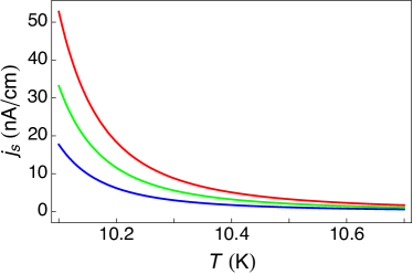
Figure 1: Photogalvanic current of fluctuating Cooper pairs [Eq. (IV) where $\Lambda$ is replaced with $\Lambda_{\tau}$] as a function of temperature for $\omega=0.1$ ps^-1 and various relaxation times: $\tau=5\,{\rm ps}$ (red), $\tau=0.3\,{\rm ps}$ (green), and $\tau=0.1\,{\rm ps}$ (blue). All parameters are for MoS₂: superconducting critical temperature $T_{c}=10\,{\rm K}$, the warping amplitude $w=3.4\,{\rm eV}\cdot\textrm{\AA}^{3}$, $\lambda_{c}=3\,{\rm meV}$, $B=1\,{\rm T}$, and the amplitude of electromagnetic field is $E_{0}=1\,{\rm V/cm}$.

Figure 1 and Fig. 2 show the temperature and frequency dependencies of the PGE current. Red curves correspond to the case of a clean superconductor, $\tau T_{c}\gg 1$. In terms of the EM field intensity, $I=c\epsilon_{0}|\textbf{E}|^{2}/2$ with $c$ the speed of light and $\epsilon_{0}$ the vacuum permittivity, the estimation gives $j/I\approx 4\,\textrm{nA}\cdot\textrm{cm}/\textrm{W}$ for $T=10.1\,\textrm{K}$ and $B=1\,\textrm{T}$. Green and blue curves correspond to the case of dirty superconductors, $\tau T_{c}\ll 1$ and demonstrate the effect of the point-like impurities on the temperature and frequency dependencies of the PGE contribution due to SC fluctuations.

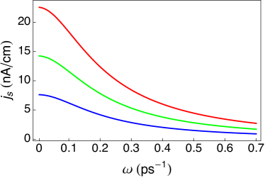
Figure 2: Photogalvanic current of fluctuating Cooper pairs [Eq. (IV) where $\Lambda$ is replaced with $\Lambda_{\tau}$] as a function of electromagnetic field frequency for $T=10.2\,\textrm{K}$ and various relaxation times: $\tau=5\,{\rm ps}$ (red), $\tau=0.3\,{\rm ps}$ (green), and $\tau=0.1\,{\rm ps}$ (blue). All other parameters are the same as in Fig. 1.

Conclusions

We conclude, that in a two-dimensional noncentrosymmetric fluctuating Ising superconductor possessing trigonal warping of the valleys and exposed to a uniform external electromagnetic field there emerge two contributions to the photogalvanic effect. The first contribution originates from the normal-state electron gas in the presence of Coulomb impurities in the sample. The second contribution stems from the presence of superconducting fluctuations. In order to lift the valley degeneracy and, thus, have a nonzero photogalvanic electric current in the system, it is sufficient to use a weak out-of-plane external magnetic field producing a Zeeman effect and breaking the time-reversal symmetry.

The photogalvanic effect, thus, possesses Aslamazov-Larkin nature since it originates from the presence of fluctuating Cooper pairs when the ambient temperature approaches the temperature of superconducting transition in the sample. The electric current, as a second-order response of the system, possesses, first, a more pronounced temperature divergence $(T-T_{c})^{-2}$, as compared with the Aslamazov-Larkin correction to the Drude conductivity, and, second, the current density has no smallness related to the electron-hole asymmetry of the quasiparticle spectrum, as it takes place in other second-order response effects [35, 36, 37].

References

- Glazov and Ganichev [2014] M. Glazov and S. Ganichev, Physics Reports 535, 101 (2014).
- Sturman and Fridkin [1992] B. I. Sturman and V. Fridkin, The photovoltaic and photorefractive effects in non-centrosymmetric materials (Gordon and Breach, New York, 1992).
- Ivchenko [2005] E. L. Ivchenko, Optical spectroscopy of semiconductor nanostructures (Alpha Science International, Harrow, UK, 2005).
- Ganichev and Prettl [2006] S. D. Ganichev and W. Prettl, Intense Terahertz Excitation of Semiconductors (Oxford Univ. Press, Oxford, 2006).
- Wang et al. [2012] Q. H. Wang, K. Kalantar-Zadeh, A. Kis, J. N. Coleman, and M. S. Strano, Nature Nanotechnology 7, 699 (2012).
- Manzeli et al. [2017] S. Manzeli, D. Ovchinnikov, D. Pasquier, O. V. Yazyev, and A. Kis, Nature Reviews Materials 2, 1 (2017).
- Entin et al. [2019] M. V. Entin, L. I. Magarill, and V. M. Kovalev, Journal of Physics: Condensed Matter 31, 325302 (2019).
- Kovalev and Savenko [2019] V. M. Kovalev and I. G. Savenko, Phys. Rev. B 99, 075405 (2019).
- Entin and Kovalev [2021] M. V. Entin and V. M. Kovalev, Phys. Rev. B 104, 075424 (2021).
- Ye et al. [2012] J. T. Ye, Y. J. Zhang, R. Akashi, M. S. Bahramy, R. Arita, and Y. Iwasa, Science 338, 1193 (2012).
- Lu et al. [2015] J. M. Lu, O. Zheliuk, I. Leermakers, N. F. Q. Yuan, U. Zeitler, K. T. Law, and J. T. Ye, Science 350, 1353 (2015).
- Costanzo et al. [2016] D. Costanzo, S. Jo, H. Berger, and A. F. Morpurgo, Nature Nanotechnology , 339 (2016).
- Sun et al. [2021] M. Sun, A. V. Parafilo, K. H. A. Villegas, V. M. Kovalev, and I. G. Savenko, 2D Materials 8, 031004 (2021).
- Sun et al. [2019] M. Sun, K. H. A. Villegas, V. M. Kovalev, and I. G. Savenko, Phys. Rev. B 99, 115408 (2019).
- Villegas et al. [2020] K. H. A. Villegas, F. V. Kusmartsev, Y. Luo, and I. G. Savenko, Phys. Rev. Lett. 124, 087701 (2020).
- Aslamazov and Larkin [1968] L. G. Aslamazov and A. I. Larkin, Fiz. Tverd. Tela 10, 1104 (1968).
- Larkin and Varlamov [2005] A. Larkin and A. Varlamov, Theory of Fluctuations in Superconductors (Oxford University Press, 2005).
- Kovalev and Savenko [2020] V. M. Kovalev and I. G. Savenko, Phys. Rev. Lett. 124, 207002 (2020).
- Saito et al. [2016] Y. Saito, T. Nojima, and Y. Iwasa, Nature Reviews Materials 2, 16094 (2016).
- Xi et al. [2016] X. Xi, Z. Wang, W. Zhao, J.-H. Park, K. T. Law, H. Berger, L. Forró, J. Shan, and K. F. Mak, Nature Physics 12, 139 (2016).
- Yuan et al. [2014] N. F. Q. Yuan, K. F. Mak, and K. T. Law, Phys. Rev. Lett. 113, 097001 (2014).
- Li et al. [2021] W. Li, J. Huang, X. Li, S. Zhao, J. Lu, Z. V. Han, and H. Wang, Materials Today Physics 21, 100504 (2021).
- Wakatsuki et al. [2017] R. Wakatsuki, Y. Saito, S. Hoshino, Y. M. Itahashi, T. Ideue, M. Ezawa, Y. Iwasa, and N. Nagaosa, Science Advances 3, e1602390 (2017).
- Hoshino et al. [2018] S. Hoshino, R. Wakatsuki, K. Hamamoto, and N. Nagaosa, Phys. Rev. B 98, 054510 (2018).
- Zaitsev [2014] R. O. Zaitsev, Introduction to modern kinetic theory (URSS editorial, 2014).
- Ziman [2001] J. Ziman, Electrons and Phonons: The Theory of Transport Phenomena in Solids (Oxford University Press, Oxford, 2001).
- Kaasbjerg et al. [2019] K. Kaasbjerg, T. Low, and A.-P. Jauho, Phys. Rev. B 100, 115409 (2019).
- [28] .
- Kormányos et al. [2015] A. Kormányos, G. Burkard, M. Gmitra, J. Fabian, V. Zólyomi, N. D. Drummond, and V. Fal’ko, 2D Materials 2, 022001 (2015).
- Aronov et al. [1995] A. G. Aronov, S. Hikami, and A. I. Larkin, Phys. Rev. B 51, 3880 (1995).
- Maki [1968] K. Maki, Prog. Theor. Phys. 40, 193 (1968).
- Thompson [1970] R. S. Thompson, Phys. Rev. B 1, 327 (1970).
- Aslamazov and Larkin [1974] L. G. Aslamazov and A. I. Larkin, Zh. Eksp. Teor. Fiz. 67, 647 (1974).
- Levanyuk [1959] A. Levanyuk, Sov. Phys. JETP 9, 571 (1959).
- Kamenev and Oreg [1995] A. Kamenev and Y. Oreg, Phys. Rev. B 52, 7516 (1995).
- Mironov et al. [2021] S. V. Mironov, A. S. Mel’nikov, I. D. Tokman, V. Vadimov, B. Lounis, and A. I. Buzdin, Phys. Rev. Lett. 126, 137002 (2021).
- Boev [2020] M. V. Boev, Phys. Rev. B 101, 104512 (2020).