Residual flavor symmetry breaking in the landscape of modular flavor models

Abstract

We study a symmetry breaking of residual flavor symmetries realized at fixed points of the moduli space. In the supersymmetric modular invariant theories, a small departure of the modulus from fixed points is required to realize fermion mass hierarchies and sizable CP-breaking effects. We investigate whether one can dynamically fix the moduli values in the vicinity of the fixed points in the context of Type IIB string theory. It is found that the string landscape prefers $|\delta\tau|\simeq 10^{-5}$ for the deviation of the complex structure modulus from all fixed points and the CP-breaking vacuum is statistically favored. To illustrate phenomenological implications of distributions of moduli values around fixed points, we analyze the lepton sector on a concrete $A_{4}$ modular flavor model.

1 Introduction

The flavor symmetry is a powerful approach to understand the flavor structure of quarks and leptons, and in addition, it provides the bridge between bottom-up and top-down approaches of model building. Indeed, when the flavor symmetry is embedded into a geometric symmetry of an extra-dimensional space, subgroups of the geometric symmetry would control the flavor structure of matter zero-modes. For instance, the $PSL(2,\mathbb{Z})$ modular symmetry incorporates the phenomenologically interesting non-Abelian discrete symmetries such as $S_{3},S_{4},A_{4}$ and $A_{5}$ in the principal subgroups deAdelhartToorop:2011re . From the viewpoint of ultraviolet physics, it was known that the $SL(2,\mathbb{Z})$ modular group and its subgroups appearing in toroidal compactifications are connected to the flavor symmetries of matter zero-modes in heterotic orbifold models Ferrara:1989qb ; Lerche:1989cs ; Lauer:1990tm ; Baur:2019kwi ; Baur:2019iai and Type IIB superstring theories with magnetized D-branes Kobayashi:2018rad ; Kobayashi:2018bff ; Ohki:2020bpo ; Kikuchi:2020frp ; Kikuchi:2020nxn ; Kikuchi:2021ogn ; Almumin:2021fbk . Such flavor symmetries are called modular flavor symmetries. The multi moduli cases such as $Sp(2h,\mathbb{Z})$ symplectic modular symmetry are also discussed in the context of heterotic string theory on toroidal orbifolds Baur:2020yjl and Calabi-Yau manifolds Strominger:1990pd ; Candelas:1990pi ; Ishiguro:2020nuf ; Ishiguro:2021ccl .

From the phenomenological point of view, the modular flavor symmetries are attractive for predicting the masses and mixing angles of quarks and leptons under a certain value of the moduli fields Feruglio:2017spp ; Kobayashi:2018vbk ; Penedo:2018nmg ; Novichkov:2018nkm ; Ding:2019xna ; Liu:2019khw ; Chen:2020udk ; Novichkov:2020eep ; Liu:2020akv ; Wang:2020lxk ; Yao:2020zml ; Ding:2020msi . The higher-dimensional operators in the Standard Model effective field theory are also controlled by the modular symmetries Kobayashi:2021pav ; Kobayashi:2022jvy , taking into account the selection rule of the string theory Kobayashi:2021uam . The flavor symmetry of quarks/leptons, as well as CP symmetry, is broken only by the modulus $\tau$ parametrizing the shape of the torus. Note that the CP transformation is regarded as an outer automorphism of the modular group for the single modulus Baur:2019kwi ; Novichkov:2019sqv and multi moduli cases Ishiguro:2021ccl . Once the modulus is fixed, there is no flavor symmetry in a generic moduli space. However, there exist so-called fixed points in the fundamental region of the $PSL(2,\mathbb{Z})$: $\tau=i,w,i\infty$ with $w=\frac{-1+i\sqrt{3}}{2}$, preserving $\mathbb{Z}_{2}$, $\mathbb{Z}_{3}$ and $\mathbb{Z}_{2}$ symmetries, respectively. Such fixed points play an important role for several phenomenological applications of the lepton sector Novichkov:2018ovf ; Novichkov:2018yse ; Novichkov:2018nkm ; Ding:2019gof ; Okada:2019uoy ; King:2019vhv ; Okada:2020rjb ; Okada:2020ukr ; Okada:2020brs ; Feruglio:2021dte ; Kobayashi:2021pav ; Kobayashi:2022jvy as well as controlling the effective action such as the dark matter (DM) stability Kobayashi:2021ajl . To dynamically fix the moduli values gives a strong prediction on proposed modular flavor models. These attempts were performed in Refs. Kobayashi:2019xvz ; Kobayashi:2019uyt ; Kobayashi:2020uaj ; Ishiguro:2020tmo ; Novichkov:2022wvg . However, in most of modular flavor models, one requires a slight difference in moduli values from fixed points to explain the observed masses and mixing angles of quarks/leptons as recently discussed in Ref. Novichkov:2022wvg .

In this paper, we adopt a top-down approach to dynamically fix the moduli values around the fixed points of the moduli space. In the string theory, background fluxes can stabilize the moduli fields such that subgroups of $SL(2,\mathbb{Z})$ are realized Kobayashi:2020hoc and also the CP symmetry is spontaneously broken Kobayashi:2020uaj ; Ishiguro:2020nuf . In addition, the flux landscape prefers the stabilization of moduli fields at fixed points with enhanced symmetries DeWolfe:2004ns ; Ishiguro:2020tmo . The purpose of this paper is to investigate the stabilization of moduli values at nearby fixed points and discuss the phenomenological implications. For concreteness, we focus on Type IIB string theory on toroidal orientifolds, where the complex structure moduli determine the flavor structure of quarks and leptons. Turning on background three-form fluxes, these complex structure moduli, as well as the dilaton, will be stabilized at statistically-favored symmetric points. To break enhanced symmetries in the complex structure moduli space, we incorporate non-perturbative effects whose existence is motivated by the stabilization of remaining volume moduli associated with the metric of extra-dimensional space. It is then expected that these non-perturbative effects can slightly shift the values of complex structure moduli from fixed points. Indeed, our systematic analysis of flux vacua with non-perturbative effects reveals that the complex structure moduli are stabilized at nearby fixed points whose magnitudes are controlled by non-perturbative effects.

Furthermore, we also incorporate the uplifting potential to obtain the de Sitter (dS) vacuum as discussed in the Kachru-Kallosh-Linde-Trivedi (KKLT) scenario Kachru:2003aw . Such a supersymmetry (SUSY) breaking source also shift the value of the complex structure moduli from fixed points. It turns out that the string landscape prefers $|\delta\tau|\simeq 10^{-5}$ for the deviation of the complex structure modulus from fixed points $\langle\tau\rangle=i,w,2i$, respectively. It corresponds to a specific SUSY breaking scale. In addition, the CP-breaking vacua are statistically favored due to the existence of non-perturbative effects as well as the uplifting source, although the number of CP-breaking vacua is statistically small in the finite number of flux vacua Ishiguro:2020tmo . These moduli values are well fitted with observed masses and mixing angles in the lepton sector on a concrete $A_{4}$ modular flavor model. Furthermore, a quasi-stable dark matter (DM) would be realized due to the softly broken residual flavor symmetry at fixed points.

This paper is organized as follows. After reviewing the structure of Type IIB flux vacua on $T^{6}/(\mathbb{Z}_{2}\times\mathbb{Z}_{2}^{\prime})$ orientifolds in section 2.1, we incorporate the non-perturbative effects to stabilize the volume moduli in section 2.2. We numerically estimate the deviations of the complex structure modulus $\tau$ from fixed points in section 2.3, taking into account SUSY breaking effects. These effects slightly break the enhanced symmetries in the moduli space of toroidal orientifolds. Given these moduli values, we study the concrete $A_{4}$ modular flavor model in section 3 with an emphasis on the lepton sector. The distributions of $A_{4}$ model and the string landscape are compared. We summarize the paper in section 4. In Appendix A, we list the $A_{4}$ modular forms used in this paper.

2 Moduli distributions in the string landscape

In section 2.1, we first review the flux vacua in Type IIB string theory on $T^{6}/(\mathbb{Z}_{2}\times\mathbb{Z}_{2}^{\prime})$ orientifolds with an emphasis on the enhanced symmetry in the complex structure moduli space. Next, we focus on non-perturbative effects, which slightly break the enhanced symmetries in moduli space of toroidal orbifolds as discussed in section 2.2. Finally, we plot the deviation of the complex structure modulus from fixed points and the typical SUSY breaking scale in section 2.3.

2.1 Flux vacua with enhanced symmetries

In Type IIB string theory on $T^{6}/(\mathbb{Z}_{2}\times\mathbb{Z}_{2}^{\prime})$ orientifolds, the moduli Kähler potential and the flux-induced superpotential are given by

$$K =-\ln(-i(S-\bar{S}))-2\ln{\cal V}(T)-3\ln\left(i(\tau-\bar{\tau})\right),$$ (2.1)

where $S,T,\tau$ denote the dilaton, Kähler moduli (volume moduli) and the complex structure modulus, respectively. Here and in what follows, we adopt the reduced Planck mass unit unless we specify it, and we consider the isotropic torus $\tau=\tau_{1}=\tau_{2}=\tau_{3}$ to simplify our analysis. In Type IIB flux compactifications, one can consider the so-called Gukov-Vafa-Witten type superpotential Gukov:1999ya induced by background three-form fluxes:

$$W_{\rm flux} =a^{0}\tau^{3}-3a\tau^{2}-3b\tau-b_{0}-S\left(c^{0}\tau^{3}-3c\tau^{2}-3d\tau-d_{0}\right),$$ (2.2)

where $\{a^{0},a,b,b_{0},c^{0},c,d,d_{0}\}$ represent three-form flux quanta with the notation of Ref. Ishiguro:2020tmo . These integers are now quantized in multiple of 8 on $T^{6}/(\mathbb{Z}_{2}\times\mathbb{Z}_{2}^{\prime})$ geometry. In this paper, we analyze the SUSY minima:

$$\partial_{S}W=\partial_{\tau}W=W=0\,,$$ (2.3)

at which the energy of scalar potential vanishes $V=e^{K}(K^{I\bar{J}}D_{I}W\overline{D_{J}W}-3|W|^{2})=0$ with $D_{I}W=\partial_{I}W+W\partial_{I}K$. Here, we use the so-called no-scale structure for the Kähler moduli: $K^{i\bar{j}}K_{i}K_{\bar{j}}=3$ with $K_{i}=\partial_{T^{i}}K$ and $K^{i\bar{j}}$ being the inverse of Kähler metric. The SUSY conditions can be analytically solved by redefining the superpotential as

$$W_{\rm RR}=a^{0}\tau^{3}-3a\tau^{2}-3b\tau-b_{0}=(r\tau+s)P(\tau)\,,$$ (2.4)

$$W_{\rm NS}=c^{0}\tau^{3}-3c\tau^{2}-3d\tau-d_{0}=(u\tau+v)P(\tau)\,.$$ (2.5)

Here, we denote a quadratic (integer-coefficient) polynomial $P(\tau)$ with respect to $\tau$, and the minimum of $\tau$ is found by solving $P(\tau)=0$. Following Ref. Betzler:2019kon , we write

$$P(\tau)=l\tau^{2}+m\tau+n\,,$$ (2.6)

under $m^{2}-4ln<0$, whose expression leads to the vacuum expectation value of $\tau$:

$$\langle\tau\rangle =\frac{-m+\sqrt{m^{2}-4ln}}{2l}\quad(l,n>0)\,,$$

$$\langle\tau\rangle =\frac{-m-\sqrt{m^{2}-4ln}}{2l}\quad(l,n<0)\,.$$ (2.7)

The vacuum expectation value of the dilaton field is obtained by solving $\partial_{\tau}W=0$, i.e.,

$$P(\tau)\partial_{\tau}\{(r\tau+s)-S(u\tau+v)\}+\{(r\tau+s)-S(u\tau+v)\}\partial_{\tau}P(\tau)=0\,.$$ (2.8)

Since the $\tau$ is now stabilized at Eq. (2.7) determined by $P(\tau)=0$, we require

$$\langle S\rangle=\frac{r\tau+s}{u\tau+v}\,.$$ (2.9)

Note that the condition $\partial_{\tau}P(\tau)=0$ gives rise to a real $\tau$ and the dilaton cannot be stabilized anymore. At this stage, one cannot stabilize the Kähler moduli and requires additional sources such as non-perturbative effects.

Before going into the detail of the volume moduli stabilization, we also review the structure of flux vacua on the toroidal orientifold. Remarkably, the background three-form fluxes induce a net D3-brane charge:

$$N_{\rm flux} =\frac{1}{l_{s}^{4}}\int H_{3}\wedge F_{3}=c^{0}b_{0}-d_{0}a^{0}+\sum_{i=1}^{3}(c^{i}b_{i}-d_{i}a^{i})=c^{0}b_{0}-d_{0}a^{0}+3(cb-da)\,,$$ (2.10)

with the string length $l_{s}$, which should be canceled on a compact manifold. Taking into the contributions of D3/D7-branes and O3/O7-planes, the flux-induced D3-brane charge is constrained as

$$0\leq N_{\rm flux}\leq N_{\rm flux}^{\rm max}={\cal O}(10^{5})\,.$$ (2.11)

Here, we admit the F-theory extension of the Type IIB orientifolds where a largest value of O3-plane contribution is given by $1820448$ Candelas:1997eh ; Taylor:2015xtz . Furthermore, $N_{\rm flux}$ should be in multiple of 192 due to the fact that $\{a^{0},a,b,b_{0},c^{0},c,d,d_{0}\}\in 8\mathbb{Z}$.

For concreteness, we focus on the vacuum structure of $\tau$ whose fixed points in the moduli space are $\tau=i,w=\frac{-1+i\sqrt{3}}{2},i\infty$, each of which corresponds to the $\mathbb{Z}_{2}$, $\mathbb{Z}_{3}$, $\mathbb{Z}_{2}$ fixed points, respectively. The $\tau=i,w$ fixed points are statistically favored in the flux landscape, as seen in Fig. 1, where the higher the degeneracy of vacua, the darker the color is. Note that one cannot realize $\tau=i\infty$ requiring the infinite value of flux quanta, and it is inconsistent with the charge cancellation condition of D3-brane charge (2.11), namely the tadpole cancellation condition. In this respect, we adopt $\tau=2i$ as an approximation of $\tau=i\infty$. Such an approximation will often be used in the phenomenological analysis of modular flavor models.

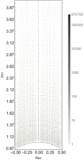
Figure 1: The numbers of stable vacua on the fundamental domain of $\tau$ in the case of $N_{\rm flux}^{\rm max}=192\times 1000$ Ishiguro:2020tmo .

2.2 Stabilization of volume moduli by non-perturbative effects

In this section, we analyze the stabilization of volume moduli along the line of KKLT scenario Kachru:2003aw . The stabilization of volume moduli is performed by the following non-perturbative effects:

$$W=W_{\rm flux}(\tau,S)+W_{\rm np}(S,T)\,,$$ (2.12)

where

$$W_{\rm np}=\sum_{m}C_{m}e^{ia_{m}T+ib_{m}S}$$ (2.13)

is supposed to be generated by D-brane instanton effects with $a_{m},b_{m}=2\pi$ or strong dynamics on D7-branes wrapping the rigid cycle with $a_{m}=2\pi/N$ and $N$ being the rank of the gauge group. Here and in what follows, we consider a simple setup where the volume of internal manifold is determined by a single Kähler modulus $T$ whose Kähler potential is given by $K=-3\ln(i(\bar{T}-T))$.

In the KKLT construction, the dilaton and the complex structure moduli are determined in the context of Type IIB flux compactifications as discussed in section 2.1. Note that the vacuum expectation value of flux superpotential vanishes in our analysis in the previous section; thereby the dilaton-dependent non-perturbative effects would induce the constant term in the effective superpotential:

$$W_{\rm eff}=W_{\rm np}(\langle S\rangle,T)\,,$$ (2.14)

which includes the following terms required in the KKLT construction:

$$W_{\rm eff}\simeq\langle e^{ibS}\rangle+Ce^{iaT}\,.$$ (2.15)

Thus, the overall Kähler modulus is stabilized at $T=T_{0}$ satisfying

$$D_{T}W_{\rm eff}=\partial_{T}W_{\rm eff}+K_{T}W_{\rm eff}=0\,,$$ (2.16)

at which the minimum value of $T$ is estimated as

$$a\langle T\rangle\approx\ln(C/w_{0})\,,$$ (2.17)

with $w_{0}=\langle e^{ibS}\rangle$. Here, the origin of small superpotential $w_{0}$ relies on the dilaton-dependent non-perturbative effects. It is also possible to realize the small flux superpotential in Type IIB/F-theory flux compactifications (see, Refs. Demirtas:2019sip ; Honma:2021klo , for the large complex structure regime). In what follows, the prefactor $C$ is assumed to be a constant, in particular, 1.

So far, we have assumed that the dilaton and the complex structure moduli are stabilized in flux compactifications. However, the presence of non-perturbative effects slightly shifts their values. Indeed, the true vacuum is found by solving

$$D_{I}W=0\,,$$ (2.18)

which changes the moduli values obtained in the previous section. To find the slight difference from the fixed points of complex structure modulus, we utilize the perturbation method; the non-perturbative superpotential $W_{\rm np}$ causes the shift of the minima:

$$\tau =\langle\tau\rangle+\delta\tau\,,$$

$$S =\langle S\rangle+\delta S\,,$$

$$T =\langle T\rangle+\delta T\,,$$ (2.19)

where the reference points $\{\langle\tau\rangle,\langle S\rangle,\langle T\rangle\}$ are given in Eqs. (2.7), (2.9) and (2.17), respectively.

Following Ref.Abe:2006xi , we estimate the deviation up to a linear order. Let us consider the Kähler-invariant quantity $G=K+\ln|W|^{2}$ satisfying $G_{A}=\partial_{A}G=0$ at the SUSY minima. Here and in what follows, the index $A$ denotes both the holomorphic and anti-holomorphic fields: $\{S,T,\tau,\bar{S},\bar{T},\bar{\tau}\}$. From the expansion (2.19), $G_{A}$ is expanded as

$$G_{A}=G_{A}\bigl{|}_{\langle\rangle}+\delta\phi^{B}G_{AB}\bigl{|}_{\langle\rangle}+({\cal O}(\delta\phi)^{2})\,,$$ (2.20)

where $\bigl{|}_{\langle\rangle}$ means $\bigl{|}_{\tau=\langle\tau\rangle,S=\langle S\rangle,T=\langle T\rangle}$. Under the assumption $a,b>1$, we obtain

$$G_{IJ},G_{\bar{I}\bar{J}}\gg G_{I\bar{J}},G_{\bar{I}J}\,,$$ (2.21)

which implies that $G_{AB}$ and $G^{AB}$ are diagonalized only by the holomorphic and anti-holomorphic parts, respectively. As a result, we obtain

$$\delta\phi^{I}=G^{IJ}G_{J}\bigl{|}_{\langle\rangle}+({\cal O}(\delta\phi)^{2})\,,$$ (2.22)

whose explicit form is written by

$$\delta\tau =W_{\rm eff}\left(-\frac{G_{S}}{W_{S\tau}}\right)\biggl{|}_{\langle\rangle}+{\cal O}(W_{\rm eff}^{2})\,,$$

$$\delta S =\frac{W_{\rm eff}}{W_{S\tau}}\left(\frac{W_{\tau\tau}}{W_{S\tau}}G_{S}-G_{\tau}\right)\biggl{|}_{\langle\rangle}+{\cal O}(W_{\rm eff}^{2})\,,$$

$$\delta T =\left(-\frac{G_{ST}}{G_{TT}}\right)\biggl{|}_{\langle\rangle}\delta S\,.$$ (2.23)

Note that the internal volume should be larger than the string length,

$${\rm Im}(T)\gg 1\,,$$ (2.24)

and the weak string coupling ${\rm Im}(S)>1$; thereby the magnitude of the flux superpotential is exponentially small:

$$\langle W_{\rm eff}\rangle\simeq w_{0}+e^{iaT}<10^{-3}\,.$$ (2.25)

Here and in the following numerical calculations, we take $a=b=2\pi$ for concreteness.

In this way, the deviation of the vacuum values $\{\delta\tau,\delta S,\delta T\}$ are determined by the non-perturbative effects, implying that the deviation is naturally suppressed with respect to the volume modulus. From the phenomenological point of view, such a small deviation of $\tau$ is useful for predicting the masses and mixing angles of quarks and leptons, as discussed in detail in section 3. Before going into a phenomenological analysis, we discuss the supersymmetry breaking effects in the next section.

2.3 Moduli values at nearby fixed points

So far, we have analyzed the stabilization of the complex structure modulus, dilaton and Kähler moduli at SUSY minima. However, the obtained vacuum energy is negative, i.e., anti-de Sitter (AdS) vacuum. To realize a dS vacuum, it is required to uplift the AdS vacuum to the dS one. Among several proposals for the uplifting scenarios, we focus on the anti D3-brane as originally utilized in the KKLT scenario Kachru:2003aw . The anti D3-brane induces the positive vacuum energy due to its SUSY breaking effect,

$$V_{\rm up}=\frac{D}{(i(\bar{T}-T))^{3}}\,,$$ (2.26)

where a constant $D$ is chosen to realize the present vacuum energy. Then, the effective scalar potential is described as

$$V=e^{K}\left(K^{I\bar{J}}D_{I}W\overline{D_{J}W}-3|W|^{2}\right)+V_{\rm up}\,,$$ (2.27)

indicating that the uplifting source further causes the shift of the moduli values obtained in the previous section.

To see the deviation of complex structure moduli values from fixed points, we numerically calculate the deviation of $\tau$ from $\langle\tau\rangle=i,w,2i$ by utilizing a finite number of flux vacua with $N_{\rm flux}^{\rm max}=1000$. By calculating the minimization condition of the full scalar potential $\partial_{I}V=0$ for $I=\tau,S,T$, we find deviations of the complex structure modulus from fixed points $\delta\tau\equiv\tau-\langle\tau\rangle$ as shown in Figs. 2, 3 and 4. It turns out that the flux landscape prefers $|\delta\tau|\simeq 10^{-5}$ from fixed points $\langle\tau\rangle=i,w,2i$, but there is no sizable difference in the phase direction. It means that the CP symmetry parametrized by $\tau\rightarrow-\bar{\tau}$ is broken in a generic moduli space. Furthermore, we plot the typical SUSY breaking scale, i.e., the gravitino mass $m_{3/2}=e^{K/2}W$, in the same figures. At the statistically favored moduli values $|\delta\tau|={\cal O}(10^{-5})$, the gravitino mass is $m_{3/2}={\cal O}(10^{-5})$ in the reduced Planck mass unit. Note that the small $\delta\tau$ is originating from non-perturbative effects and the uplifting source, both of which are the same order.

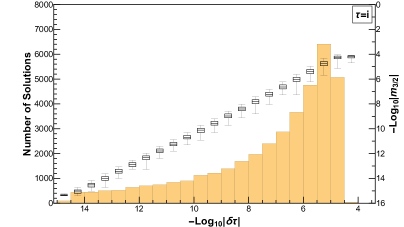
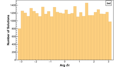
Figure 2: The number of vacua at nearby $\langle\tau\rangle=i$ as a function of $|\delta\tau|$ in the left panel and ${\rm Arg}(\delta\tau)$ in the right panel, respectively. In the left panel, the absolute value of gravitino mass is plotted as a function of $|\delta\tau|$.

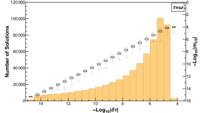
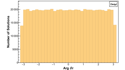
Figure 3: The number of vacua at nearby $\langle\tau\rangle=w$ as a function of $|\delta\tau|$ in the left panel and ${\rm Arg}(\delta\tau)$ in the right panel, respectively. In the left panel, the absolute value of gravitino mass is plotted as a function of $|\delta\tau|$.

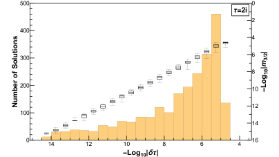
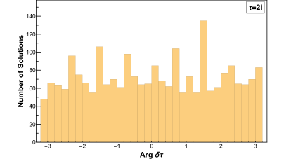
Figure 4: The number of vacua at nearby $\langle\tau\rangle=2i$ as a function of $|\delta\tau|$ in the left panel and ${\rm Arg}(\delta\tau)$ in the right panel, respectively. In the left panel, the absolute value of gravitino mass is plotted as a function of $|\delta\tau|$.

3 $A_{4}$ modular flavor model

To illustrate implications of distributions of moduli fields around fixed points, we study the phenomenology of lepton sector on a concrete $A_{4}$ modular flavor model.

3.1 Setup

	$L$	$\{e^{c},\mu^{c},\tau^{c}\}$	$N^{c}$	$H_{u}$	$H_{d}$
$SU(2)_{L}$	$\bf{2}$	$\bf{1}$	$\bf{1}$	$\bf{2}$	$\bf{2}$
$U(1)_{Y}$	$-\frac{1}{2}$	$1$	$0$	$\frac{1}{2}$	$-\frac{1}{2}$
$A_{4}$	${\bf 3}$	$\{\bf 1,1^{\prime},1^{\prime}\}$	${\bf 3}$	${\bf 1}$	${\bf 1}$
$-k_{I}$	$-2$	$\{-2,-4,-4\}$	$-2$	$0$	$0$

Table 1: Charge assignments under $SU(2)_{L}\times U(1)_{Y}\times A_{4}$ in the lepton and Higgs sectors, where $k_{I}$ denotes the modular weight of matter superfields $\Phi_{I}$.

For concreteness, we specify charge assignments under $SU(2)_{L}\times U(1)_{Y}\times A_{4}$ for the lepton and Higgs sectors as summarized in Tab. 1. Here, the $A_{4}$ group belongs to the $SL(2,\mathbb{Z})$ modular group parametrized by the modulus $\tau$. The Yukawa couplings are constructed in a modular invariant way. (For more details, see, Appendix A.) Then, we can write down the modular invariant superpotential:

$$W =y_{e}(Y_{\bf 3}^{(4)}L)_{1}H_{d}e^{c}+\sum_{\bf r=3,3^{\prime}}y_{\mu}^{({\bf r})}(Y_{\bf r}^{(6)}L)_{1}H_{d}\mu^{c}+\sum_{\bf r=3,3^{\prime}}y_{\tau}^{({\bf r})}(Y_{\bf r}^{(6)}L)_{1}H_{d}\tau^{c}$$

$$+\sum_{\bf r=1,1^{\prime}}y_{d}^{({\bf r})}(Y_{\bf r}^{(4)}LH_{u}N^{c})_{1}+y_{d}^{({\bf 3_{S}})}(Y_{\bf 3}^{(4)}H_{u}(LN^{c})_{\bf 3_{S}})_{1}+y_{d}^{({\bf 3_{A}})}(Y_{\bf 3}^{(4)}H_{u}(LN^{c})_{\bf 3_{A}})_{1}$$

$$+\sum_{\bf r=1,1^{\prime},3}M^{({\bf r})}(Y_{\bf r}^{(4)}N^{c}N^{c})_{1},$$ (3.1)

where $Y_{\bf r}^{(k)}$ denotes the holomorphic modular form with weight $k$ for ${\bf r}$ representations under the $A_{4}$ group, and $\{y_{e},y_{\mu}^{({\bf r})},y_{\tau}^{({\bf r})},y_{d}^{({\bf r})}\}$ are parameters. Here, we introduce the Majorana mass terms to realize small neutrino masses.

In the following, we enumerate the mass matrix of the lepton sector.

1. Charged-lepton mass matrix

   After the electroweak symmetry breaking, charged-lepton mass matrix is written as

   $$(m_{l})_{LR}=\frac{v_{d}}{\sqrt{2}}\begin{pmatrix}Y_{1}^{(4)}&Y_{3}^{(6)}+\epsilon_{\mu}Y_{3^{\prime}}^{(6)}&Y_{3}^{(6)}+\epsilon_{\tau}Y_{3^{\prime}}^{(6)}\\ Y_{3}^{(4)}&Y_{2}^{(6)}+\epsilon_{\mu}Y_{2^{\prime}}^{(6)}&Y_{2}^{(6)}+\epsilon_{\tau}Y_{2^{\prime}}^{(6)}\\ Y_{2}^{(4)}&Y_{1}^{(6)}+\epsilon_{\mu}Y_{1^{\prime}}^{(6)}&Y_{1}^{(6)}+\epsilon_{\tau}Y_{1^{\prime}}^{(6)}\\ \end{pmatrix}\times\begin{pmatrix}y_{e}&0&0\\ 0&y_{\mu}^{(\bf 3)}&0\\ 0&0&y_{\tau}^{(\bf 3)}\\ \end{pmatrix},$$ (3.2)

   where we introduce

   $$\langle H_{d}\rangle=v_{d},\quad\epsilon_{\mu}=\frac{y_{\mu}^{(\bf 3^{\prime})}}{y_{\mu}^{({\bf 3})}},\quad\epsilon_{\tau}=\frac{y_{\tau}^{(\bf 3^{\prime})}}{y_{\tau}^{({\bf 3})}},\quad Y_{\bf 3}^{(k)}=\begin{pmatrix}Y_{1}^{(k)}\\ Y_{2}^{(k)}\\ Y_{3}^{(k)}\\ \end{pmatrix},\quad Y_{\bf 3^{\prime}}^{(k)}=\begin{pmatrix}Y_{1^{\prime}}^{(k)}\\ Y_{2^{\prime}}^{(k)}\\ Y_{3^{\prime}}^{(k)}\\ \end{pmatrix}.$$ (3.3)

   The explicit modular forms are listed in Appendix A. Then the charged-lepton mass square eigenstate can be found by ${\rm diag}(|m_{e}|^{2},|m_{\mu}|^{2},|m_{\tau}|^{2})\equiv V^{\dagger}_{l_{L}}m_{l}^{\dagger}m_{l}V_{l_{L}}$. We numerically determine the three parameters $y_{e},y_{\mu}^{(\bf 3)},y_{\tau}^{(\bf 3)}$ to fit the three charged-lepton masses by applying the relations:

   $${\rm Tr}[m_{l}^{\dagger}m_{l}]=|m_{e}|^{2}+|m_{\mu}|^{2}+|m_{\tau}|^{2},$$ (3.4)

   $${\rm Det}[m_{l}^{\dagger}m_{l}]=|m_{e}|^{2}|m_{\mu}|^{2}|m_{\tau}|^{2},$$ (3.5)

   $$({\rm Tr}[m_{l}^{\dagger}m_{l}])^{2}-{\rm Tr}[(m_{l}^{\dagger}m_{l})^{2}]=2(|m_{e}|^{2}|m_{\nu}|^{2}+|m_{\mu}|^{2}|m_{\tau}|^{2}+|m_{e}|^{2}|m_{\tau}|^{2}).$$ (3.6)

   Therefore, input parameters are $\epsilon_{\mu},\ \epsilon_{\tau}$ in the charged-lepton sector.

2. Dirac Yukawa mass matrix

   $$(m_{D})_{LN} =\frac{v_{u}}{\sqrt{2}}\Biggl{[}\frac{y_{d}^{({\bf 3_{S}})}}{3}\begin{pmatrix}2Y_{1}^{(4)}&-Y_{3}^{(4)}&-Y_{2}^{(4)}\\ -Y_{3}^{(4)}&2Y_{2}^{(4)}&-Y_{1}^{(4)}\\ -Y_{2}^{(4)}&-Y_{1}^{(4)}&2Y_{3}^{(4)}\\ \end{pmatrix}+\frac{y_{d}^{({\bf 3_{A}})}}{2}\begin{pmatrix}0&Y_{3}^{(4)}&-Y_{2}^{(4)}\\ -Y_{3}^{(4)}&0&Y_{1}^{(4)}\\ Y_{2}^{(4)}&-Y_{1}^{(4)}&0\\ \end{pmatrix}$$

   $$\hskip 40.0pt+y_{d}^{({\bf 1})}Y_{\bf 1}^{(4)}\begin{pmatrix}1&0&0\\ 0&0&1\\ 0&1&0\\ \end{pmatrix}+y_{d}^{({\bf 1^{\prime}})}Y_{\bf 1^{\prime}}^{(4)}\begin{pmatrix}0&0&1\\ 0&1&0\\ 1&0&0\\ \end{pmatrix}\Biggl{]}$$

   $$=m_{d_{0}}\Biggl{[}\begin{pmatrix}2Y_{1}^{(4)}&(-1+g_{D})Y_{3}^{(4)}&-(1+g_{D})Y_{2}^{(4)}\\ -(1+g_{D})Y_{3}^{(4)}&2Y_{2}^{(4)}&(-1+g_{D})Y_{1}^{(4)}\\ (-1+g_{D})Y_{2}^{(4)}&-(1+g_{D})Y_{1}^{(4)}&2Y_{3}^{(4)}\\ \end{pmatrix}$$

   $$\hskip 40.0pt+h_{1}\begin{pmatrix}1&0&0\\ 0&0&1\\ 0&1&0\\ \end{pmatrix}+h_{2}\begin{pmatrix}0&0&1\\ 0&1&0\\ 1&0&0\\ \end{pmatrix}\Biggl{]}$$

   $$\equiv m_{d_{0}}\tilde{m}_{D},$$ (3.7)

   where we define

   $$\langle H_{u}\rangle=v_{u},\quad m_{d_{0}}\equiv\frac{y_{d}^{(\bf 3_{S})}}{3\sqrt{2}}v_{u},\quad g_{D}=\frac{3y_{d}^{(\bf 3_{A})}}{2y_{d}^{(\bf 3_{S})}},\quad h_{1}=\frac{3y_{d}^{({\bf 1})}Y_{\bf 1}^{(4)}}{y_{d}^{(\bf 3_{S})}},\quad h_{2}=\frac{3y_{d}^{({\bf 1^{\prime}})}Y_{\bf 1^{\prime}}^{(4)}}{y_{d}^{(\bf 3_{S})}}.$$ (3.8)

3. Majorana mass matrix

   $$M_{N} =\frac{M_{1}}{3}\begin{pmatrix}2Y_{1}^{(4)}&-Y_{3}^{(4)}&-Y_{2}^{(4)}\\ -Y_{3}^{(4)}&2Y_{2}^{(4)}&-Y_{1}^{(4)}\\ -Y_{2}^{(4)}&-Y_{1}^{(4)}&2Y_{3}^{(4)}\\ \end{pmatrix}+M_{2}Y_{\bf 1}^{(4)}\begin{pmatrix}1&0&0\\ 0&0&1\\ 0&1&0\\ \end{pmatrix}+M_{3}Y_{\bf 1^{\prime}}^{(4)}\begin{pmatrix}0&0&1\\ 0&1&0\\ 1&0&0\\ \end{pmatrix}$$

   $$=M_{0}\Biggl{[}\begin{pmatrix}2Y_{1}^{(4)}&-Y_{3}^{(4)}&-Y_{2}^{(4)}\\ -Y_{3}^{(4)}&2Y_{2}^{(4)}&-Y_{1}^{(4)}\\ -Y_{2}^{(4)}&-Y_{1}^{(4)}&2Y_{3}^{(4)}\\ \end{pmatrix}+f_{1}\begin{pmatrix}1&0&0\\ 0&0&1\\ 0&1&0\\ \end{pmatrix}+f_{2}\begin{pmatrix}0&0&1\\ 0&1&0\\ 1&0&0\\ \end{pmatrix}\Biggl{]}$$

   $$\equiv M_{0}\tilde{M}_{N},$$ (3.9)

   where we define

   $$M_{0}\equiv\frac{M_{1}}{3},\quad f_{1}=\frac{3Y_{\bf 1}^{(4)}M_{2}}{M_{1}},\quad f_{2}=\frac{3Y_{\bf 1^{\prime}}^{(4)}M_{3}}{M_{1}}.$$ (3.10)

   Then, the active neutrino mass matrix is given by

   $$m_{\nu} \approx-m_{D}^{T}M_{N}^{-1}m_{D}=-\kappa\tilde{m}_{D}^{T}\tilde{M}_{N}^{-1}\tilde{m}_{D}=-\kappa\tilde{m}_{\nu},$$ (3.11)

   where the mass dimensional parameter $\kappa$ is defined by $m_{d_{0}}^{2}/M_{0}$. $\tilde{m}_{\nu}$ is diagonalized by applying a unitary matrix as $V^{\dagger}_{\nu}(\tilde{m}_{\nu}^{\dagger}\tilde{m}_{\nu})V_{\nu}=(\tilde{m}_{1}^{2},\tilde{m}_{2}^{2},\tilde{m}_{3}^{2})$. In this case, $\kappa$ is determined by

   $$({\rm NH}):\ \kappa^{2}=\frac{|\Delta m_{\rm atm}^{2}|}{\tilde{m}_{3}^{2}-\tilde{m}_{1}^{2}},\quad({\rm IH}):\ \kappa^{2}=\frac{|\Delta m_{\rm atm}^{2}|}{\tilde{m}_{2}^{2}-\tilde{m}_{3}^{2}},$$ (3.12)

   where $\Delta m_{\rm atm}^{2}$ is atmospheric neutrino mass square difference, and NH and IH stand for normal and inverted hierarchies, respectively. The solar mass square difference is also found in terms of $\kappa$ as follows:

   $$\Delta m_{\rm sol}^{2}={\kappa^{2}}({\tilde{m}_{2}^{2}-\tilde{m}_{1}^{2}}).$$ (3.13)

   In our numerical analysis, we regard $\Delta m_{\rm atm}^{2}$ as an input parameter from experiments so that $\Delta m_{\rm sol}^{2}$ be output parameter giving numerical $(\tilde{m}_{1}^{2},\tilde{m}_{2}^{2},\tilde{m}_{3}^{2})$. Then, one finds $U_{\rm PMNS}=V^{\dagger}_{l_{L}}V_{\nu}$, and it is parametrized by three mixing angles $\theta_{ij}(i,j=1,2,3;i<j)$, one CP violating Dirac phase $\delta_{\rm CP}$, and two Majorana phases $\{\alpha_{21},\alpha_{32}\}$ as follows:

   $$U_{\rm PMNS}=\begin{pmatrix}c_{12}c_{13}&s_{12}c_{13}&s_{13}e^{-i\delta_{\rm CP}}\\ -s_{12}c_{23}-c_{12}s_{23}s_{13}e^{i\delta_{\text{CP}}}&c_{12}c_{23}-s_{12}s_{23}s_{13}e^{i\delta_{\text{CP}}}&s_{23}c_{13}\\ s_{12}s_{23}-c_{12}c_{23}s_{13}e^{i\delta_{\text{CP}}}&-c_{12}s_{23}-s_{12}c_{23}s_{13}e^{i\delta_{\text{CP}}}&c_{23}c_{13}\end{pmatrix}\begin{pmatrix}1&0&0\\ 0&e^{i\frac{\alpha_{21}}{2}}&0\\ 0&0&e^{i\frac{\alpha_{31}}{2}}\end{pmatrix},$$ (3.14)

   where $c_{ij}$ and $s_{ij}$ stand for $\cos\theta_{ij}$ and $\sin\theta_{ij}$, respectively. These mixings are rewritten in terms of the component of $U_{\rm PMNS}$ as follows:

   $$\sin^{2}\theta_{13}=|(U_{\rm PMNS})_{13}|^{2},\quad\sin^{2}\theta_{23}=\frac{|(U_{\rm PMNS})_{23}|^{2}}{1-|(U_{\rm PMNS})_{13}|^{2}},\quad\sin^{2}\theta_{12}=\frac{|(U_{\rm PMNS})_{12}|^{2}}{1-|(U_{\rm PMNS})_{13}|^{2}}.$$ (3.15)

   In addition, we can compute the Jarlskog invariant, $\delta_{\text{CP}}$ from PMNS matrix elements $(U_{\rm PMNS})_{\alpha i}\equiv U_{\alpha i}$:

   $$J_{\rm CP}=\text{Im}[U_{e1}U_{\mu 2}U_{e2}^{*}U_{\mu 1}^{*}]=s_{23}c_{23}s_{12}c_{12}s_{13}c^{2}_{13}\sin\delta_{\rm CP},$$ (3.16)

   and the Majorana phases are also estimated in terms of other invariants $I_{1}$ and $I_{2}$ constructed by PMNS matrix elements:

   $$I_{1}=\text{Im}[U^{*}_{e1}U_{e2}]=c_{12}s_{12}c_{13}^{2}\sin\left(\frac{\alpha_{21}}{2}\right),\ I_{2}=\text{Im}[U^{*}_{e1}U_{e3}]=c_{12}s_{13}c_{13}\sin\left(\frac{\alpha_{31}}{2}-\delta_{\rm CP}\right).$$ (3.17)

   Furthermore, the effective mass for the neutrinoless double beta decay is given by

   $$\langle m_{ee}\rangle=\kappa|\tilde{D}_{\nu_{1}}c^{2}_{12}c^{2}_{13}+\tilde{D}_{\nu_{2}}s^{2}_{12}c^{2}_{13}e^{i\alpha_{21}}+\tilde{D}_{\nu_{3}}s^{2}_{13}e^{i(\alpha_{31}-2\delta_{\rm CP})}|\,,$$ (3.18)

   where its observed value could be measured by KamLAND-Zen experiment in future KamLAND-Zen:2016pfg . In our numerical analysis below, we will do $\Delta\chi$ square analysis referring to Ref. Esteban:2020cvm .

3.2 Numerical analysis

In this section, we show the allowed region with $\chi$ square analysis to satisfy the current neutrino oscillation data, where we randomly select within the following ranges of input parameters,

$$|\delta\tau|\in[10^{-20},0.1],\ \{\epsilon_{\mu},\epsilon_{\tau},g_{D},f_{1},f_{2},h_{1},h_{2}\}\in[10^{-4},2],$$ (3.19)

where we assume all the parameters (except $\tau$) are real for simplicity. We also take Yukawa couplings of the SM charged leptons at the GUT scale $2\times 10^{16}$ GeV and $\Delta m_{\rm atm}^{2}$ as input parameters, where $\tan\beta=5$ is taken as a bench mark Bjorkeroth:2015ora :

$$y_{e}=(1.97\pm 0.024)\times 10^{-6},\ y_{\mu}=(4.16\pm 0.050)\times 10^{-4},\ y_{\tau}=(7.07\pm 0.073)\times 10^{-3},$$ (3.20)

$$|\Delta m_{\rm atm}^{2}|=(2.431-2.598)\times 10^{-21}\ {\rm eV^{2}}\,\,\ {\rm for}\ {\rm NH},$$ (3.21)

$$|\Delta m_{\rm atm}^{2}|=(2.412-2.583)\times 10^{-21}\ {\rm eV^{2}}\,\,\ {\rm for}\ {\rm IH},$$ (3.22)

where the charged-lepton masses are within 1$\sigma$ region, while $\Delta m_{\rm atm}^{2}$ is within 3$\sigma$ region. Here, the lepton masses are defined by $m_{\ell}=y_{\ell}v_{H}$ with $v_{H}=174$ GeV. Then, we pick the output data up only when the $\chi$ square is within 5$\sigma$ considering five measured neutrino oscillation data; $(\Delta m^{2}_{\rm sol},\ \sin^{2}\theta_{13},\ \sin^{2}\theta_{23},\ \sin^{2}\theta_{12}$) Esteban:2018azc . Here, we do not include $\delta_{\rm CP}$ in the $\chi$ square analysis due to the large ambiguity of experimental results in $3\sigma$ interval. In general, IH case is more difficult to accumulate more data to satisfy the neutrino oscillation data, because the minimum $\chi$ square is $2.7$ in Nufit 5.0 Esteban:2018azc .

3.2.1 Nearby $\tau=i$

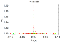
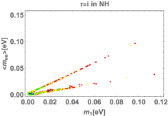
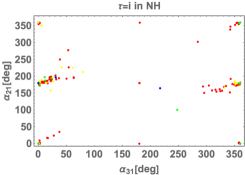
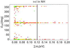
Figure 5: Each of color represents ${\rm blue}\leq 1\sigma$, $1\sigma<{\rm green}\leq 2\sigma$, $2\sigma<{\rm yellow}\leq 3\sigma$, $3\sigma<{\rm red}\leq 5\sigma$.

In Fig. 5, we show our several allowed regions on $\tau$ at nearby $\tau=i$ in case of NH, where each of color represents ${\rm blue}\leq 1\sigma$, $1\sigma<{\rm green}\leq 2\sigma$, $2\sigma<{\rm yellow}\leq 3\sigma$, $3\sigma<{\rm red}\leq 5\sigma$. The up-left one represents the allowed region of the imaginary part of $\tau$ in terms of the real part of $\tau$. The up-right one demonstrates the allowed region of neutrinoless double beta decay $\langle m_{ee}\rangle$ in terms of the lightest active neutrino mass $m_{1}$. There are two linear correlations between them. Furthermore, the smaller $\chi$ square is localized at nearby their smaller masses. The down-left one shows the allowed region of Majorana phases $\alpha_{21}$ and $\alpha_{31}$. Since we take all input parameters (except $\tau$) to be real values, both the allowed regions are localized at nearby by $0^{\circ},\ 180^{\circ}$. The down-right one depicts the allowed region of Dirac phase $\delta_{\text{CP}}$ in terms of the sum of neutrino masses $\sum m_{i}$. The vertical line is the upper bound on cosmological constraint $\sum m_{i}<0.12$ eV Planck:2018vyg . There is an intriguing tendency that allowed region of smaller $\chi$ square is localized at smaller $\sum m_{i}$ that is within the cosmological bound. Another feature is that the best fit value of Dirac CP phase $\sim 195^{\circ}$ would be reproduced when we allow up to $5\sigma$ interval.

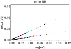
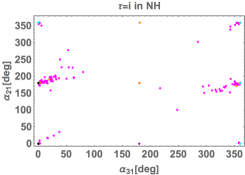
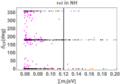
Figure 6: $|\delta\tau|<10^{-15}$ for black, $10^{-15}\leq|\delta\tau|<10^{-12}$ for gray, $10^{-12}\leq|\delta\tau|<10^{-10}$ for purple, $10^{-10}\leq|\delta\tau|<10^{-7}$ for brown, $10^{-7}\leq|\delta\tau|<10^{-5}$ for blue green, $10^{-5}\leq|\delta\tau|<10^{-3}$ for orange, and $10^{-3}\leq|\delta\tau|<10^{-1}$ for magenta.

In Fig. 6, we show the several figures in terms of deviation from $\tau=i$ in the same case of Fig. 5 at 5 $\sigma$ interval, where each of color represents $|\delta\tau|<10^{-15}$ for black, $10^{-15}\leq|\delta\tau|<10^{-12}$ for gray, $10^{-12}\leq|\delta\tau|<10^{-10}$ for purple, $10^{-10}\leq|\delta\tau|<10^{-7}$ for brown, $10^{-7}\leq|\delta\tau|<10^{-5}$ for blue green, $10^{-5}\leq|\delta\tau|<10^{-3}$ for orange, and $10^{-3}\leq|\delta\tau|<10^{-1}$ for magenta. The up-left one is the same as the case of up-right one in Fig. 5. It implies that smaller deviations $|\delta\tau|$ tend to be localized at nearby their smaller masses. The up-right one is the same as the case of down-left one in Fig. 5. This figure would show rather trivial. Therefore, the smaller deviation is localized at $0^{\circ}$ and $180^{\circ}$, while the larger deviation deviates from these two points. It directly follows from our phase source is $\tau$ only. The down-left one is the same as the case of down-right one in Fig. 5. The smaller deviation would be favored in the point of view of the bound on cosmological constraint.

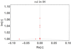
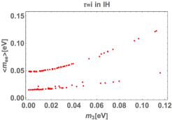
Figure 7: Each of color represents ${\rm blue}\leq 1\sigma$, $1\sigma<{\rm green}\leq 2\sigma$, $2\sigma<{\rm yellow}\leq 3\sigma$, $3\sigma<{\rm red}\leq 5\sigma$.

In Fig. 7, we show our several allowed regions on $\tau$ at nearby $\tau=i$ in case of IH, where color legends are the same as the one of Fig. 5. Therefore, we have found only the allowed region of $3\sigma-5\sigma$. The up-left one represents the allowed region of imaginary part of $\tau$ in terms of real part of $\tau$. The up-right one demonstrates the allowed region of neutrinoless double beta decay $\langle m_{ee}\rangle$ in terms of the lightest active neutrino mass $m_{3}$. There are two correlations between them; one is a linear line and another is a slightly curved one. The solutions tend to be localized at nearby smaller mass of $m_{3}$ with $\langle m_{ee}\rangle=0.015,\ 0.05$ eV. The down-left one shows the allowed region of Majorana phases $\alpha_{21}$ and $\alpha_{31}$. Both the allowed regions are localized at nearby by $0^{\circ},\ 180^{\circ}$ similar to the case of NH. The down-right one depicts the allowed region of the sum of neutrino masses $\sum m_{i}$ in terms of Dirac phase $\delta_{\text{CP}}$. The vertical line is the upper bound on cosmological constraint. $\delta_{\rm CP}$ is allowed at the points $0^{\circ}$ and $180^{\circ}$. While a large part of $\sum m_{i}$ would be ruled out by the cosmological bound. Therefore, we would predict a narrow range of $0.1~{}{\rm eV}\leq\sum m_{i}\leq 0.12~{}{\rm eV}$ in this case.

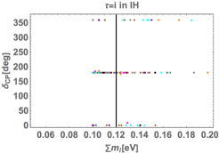
Figure 8: $|\delta\tau|<10^{-15}$ for black, $10^{-15}\leq|\delta\tau|<10^{-12}$ for gray, $10^{-12}\leq|\delta\tau|<10^{-10}$ for purple, $10^{-10}\leq|\delta\tau|<10^{-7}$ for brown, $10^{-7}\leq|\delta\tau|<10^{-5}$ for blue green, $10^{-5}\leq|\delta\tau|<10^{-3}$ for orange, and $10^{-3}\leq|\delta\tau|<10^{-1}$ for magenta.

In Fig. 8, we show the several figures in terms of deviation from $\tau=i$ where the color legends are the same as the one in Fig. 6. The up-left one corresponds to the case of up-right one in Fig. 7. It implies that smaller deviations $|\delta\tau|$ tend to be localized at nearby their smaller masses $m_{3}$. The up-right one corresponds to the case of down-left one in Fig. 7. This figure would show rather trivial. Therefore, the smaller deviation is localized at $0^{\circ}$ and $180^{\circ}$, while the larger deviation deviates from these two points. It directly follows from the fact that our phase source is $\tau$ only. The down-left one corresponds to the case of down-right one in Fig. 7. The smaller deviation would be favored in the point of view of the bound on cosmological constraint.

Finally, we discuss ratios of the number of solutions in a corresponding range of $-{\rm Log}_{10}|\delta\tau|$ to the number of whole solutions for both the string landscape in Fig. 2 and the $A_{4}$ model within $5\sigma$. Fig. 9 indicates both the distributions of $A_{4}$ model with NH and the moduli fields in the string landscape peak around $|\delta\tau|={\cal O}(10^{-5})$, but such a signal will not be found in the IH case.

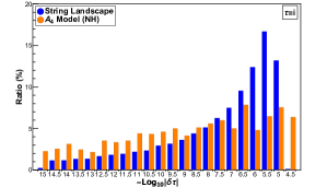
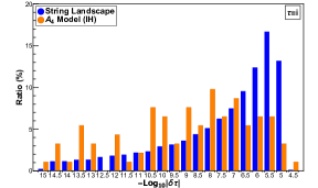
Figure 9: Ratios of the number of solutions in a corresponding range of $-{\rm Log}_{10}|\delta\tau|$ to the number of whole solutions for both the string landscape in Fig. 2 and the $A_{4}$ model within $5\sigma$. We present the NH and the IH in the left and right panels, respectively.

3.2.2 Nearby $\tau=\omega$

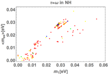
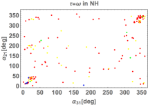
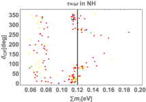
Figure 10: Each of color represents ${\rm blue}\leq 1\sigma$, $1\sigma<{\rm green}\leq 2\sigma$, $2\sigma<{\rm yellow}\leq 3\sigma$, $3\sigma<{\rm red}\leq 5\sigma$.

In Fig. 10, we show our several allowed regions on $\tau$ at nearby $\tau=\omega$ in case of NH, where the color legends are the same as the one in Fig. 6. The up-left one represents the allowed region of the imaginary part of $\tau$ in terms of the real part of $\tau$. The smaller $\chi$ square denoted by blue color is closest to the fixed point of $\tau=\omega$, which would be a good tendency. The up-right one demonstrates the allowed region of neutrinoless double beta decay $\langle m_{ee}\rangle$ in terms of the lightest active neutrino mass $m_{1}$. There is a linear correlation with width between them. Furthermore, all the regions of $\chi$ square tend to run the whole range. The down-left one shows the allowed region of Majorana phases $\alpha_{21}$ and $\alpha_{31}$. Even though the whole region is allowed, there exist two islands at around $-50^{\circ}\leq\alpha_{21},\alpha_{31}\leq 50^{\circ}$. The down-right one depicts the allowed region of Dirac phase $\delta_{\text{CP}}$ in terms of the sum of neutrino masses $\sum m_{i}$. The vertical line is the upper bound on cosmological constraint. Below this bound, the whole region is allowed for $\delta_{\rm CP}$. At nearby this bound, $\delta_{\rm CP}$ is allowed by $0^{\circ}-100^{\circ}$ and $270^{\circ}-360^{\circ}$. Furthermore, the smaller $\chi$ square tends to be localized at nearby the cosmological bound, and its testability would be enhanced.

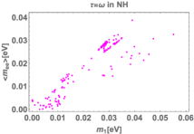
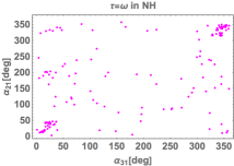
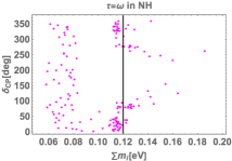
Figure 11: $|\delta\tau|<10^{-15}$ for black, $10^{-15}\leq|\delta\tau|<10^{-12}$ for gray, $10^{-12}\leq|\delta\tau|<10^{-10}$ for purple, $10^{-10}\leq|\delta\tau|<10^{-7}$ for brown, $10^{-7}\leq|\delta\tau|<10^{-5}$ for blue green, $10^{-5}\leq|\delta\tau|<10^{-3}$ for orange, and $10^{-3}\leq|\delta\tau|<10^{-1}$ for magenta.

In Fig. 11, we show the several figures in terms of deviation from $\tau=\omega$ where the color legends are the same as the one in Fig. 6. The up-left one corresponds to the case of up-right one in Fig. 10. The up-right one corresponds to the case of down-left one in Fig. 10. The down-left one corresponds to the case of down-right one in Fig. 10. These figures show us that larger deviation; $10^{-3}\leq|\delta\tau|<10^{-1}$, is requested when the neutrino oscillations are satisfied. It is not favored by the theoretical point of view as we already discussed in Sec. 2.

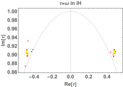
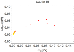
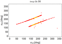
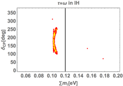
Figure 12: Each of color represents ${\rm blue}\leq 1\sigma$, $1\sigma<{\rm green}\leq 2\sigma$, $2\sigma<{\rm yellow}\leq 3\sigma$, $3\sigma<{\rm red}\leq 5\sigma$.

In Fig. 12, we show our several allowed regions on $\tau$ at nearby $\tau=\omega$ in case of IH, where the color legends are the same as the one in Fig. 6. The up-left one represents the allowed region of the imaginary part of $\tau$ in terms of the real part of $\tau$. We have found only the allowed region of $2\sigma-5\sigma$. The up-right one demonstrates the allowed region of neutrinoless double beta decay $\langle m_{ee}\rangle$ in terms of the lightest active neutrino mass $m_{3}$. There seems to be a linear correlation between them, and 0.02 eV$\lesssim\langle m_{ee}\rangle\lesssim$ 0.06 eV up to $5\sigma$, but the allowed regions are localized at nearby small masses up to $2\sigma$. The down-left one shows the allowed region of Majorana phases $\alpha_{21}$ and $\alpha_{31}$. We find the allowed regions $100^{\circ}\lesssim\alpha_{21}\lesssim 280^{\circ}$ and $50^{\circ}\lesssim\alpha_{31}\lesssim 340^{\circ}$. The down-right one depicts the allowed region of Dirac phase $\delta_{\text{CP}}$ in terms of the sum of neutrino masses $\sum m_{i}$. The allowed region at yellow plots; $\sum m_{i}\simeq 0.11$ eV, is totally within the cosmological constraint. This implies that $m_{3}$ is almost zero combined with the up-right figure.

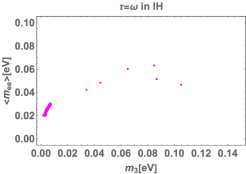
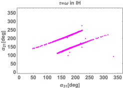
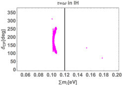
Figure 13: $|\delta\tau|<10^{-15}$ for black, $10^{-15}\leq|\delta\tau|<10^{-12}$ for gray, $10^{-12}\leq|\delta\tau|<10^{-10}$ for purple, $10^{-10}\leq|\delta\tau|<10^{-7}$ for brown, $10^{-7}\leq|\delta\tau|<10^{-5}$ for blue green, $10^{-5}\leq|\delta\tau|<10^{-3}$ for orange, and $10^{-3}\leq|\delta\tau|<10^{-1}$ for magenta.

In Fig. 13, we show the several figures in terms of deviation from $\tau=\omega$ where the color legends are the same as the one in Fig. 8. The up-left one corresponds to the case of up-right one in Fig. 12. The up-right one corresponds to the case of down-left one in Fig. 12. The down-left one corresponds to the case of down-right one in Fig. 12. These figures also show us that larger deviation; $10^{-3}\leq|\delta\tau|<10^{-1}$, is requested when the neutrino oscillations are satisfied. It is not favored by the theoretical point of view as we already discussed in Sec. 2. In conclusion, in the case of $\tau=\omega$, both the case of NH and IH would not be favored by the theoretical viewpoint.

3.2.3 Nearby $\tau=2i$

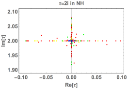
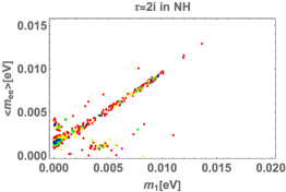
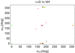
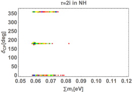
Figure 14: Each of color represents ${\rm blue}\leq 1\sigma$, $1\sigma<{\rm green}\leq 2\sigma$, $2\sigma<{\rm yellow}\leq 3\sigma$, $3\sigma<{\rm red}\leq 5\sigma$.

In Fig. 14, we show our several allowed regions on $\tau$ at nearby $\tau=2i$ in case of NH, where the color legends are the same as the one in Fig. 6. The up-left one represents the allowed region of the imaginary part of $\tau$ in terms of the real part of $\tau$. The smaller $\chi$ square denoted by blue color is closest to the fixed point of $\tau=2i$, which would be a good tendency. The up-right one demonstrates the allowed region of neutrinoless double beta decay $\langle m_{ee}\rangle$ in terms of the lightest active neutrino mass $m_{1}$. There is main linear correlation between them. We find the allowed regions 0 eV$\leq m_{1}\leq$0.014 eV, and 0 eV$\leq\langle m_{ee}\rangle\leq$0.013 eV. The down-left one shows the allowed region of Majorana phases $\alpha_{21}$ and $\alpha_{31}$. Both the phases allow to be $0^{\circ}$ or $180^{\circ}$. The down-right one depicts the allowed region of Dirac phase $\delta_{\text{CP}}$ in terms of the sum of neutrino masses $\sum m_{i}$. The whole allowed region of $\sum m_{i}$ is totally within the bound on cosmological constraint; 0.058 eV$\leq\sum m_{i}\leq$ 0.082 eV, whereas the allowed region of $\delta_{\rm CP}$ is the same as Majorana phases; $0^{\circ}$ or $180^{\circ}$. Note that it is trivial that we find no phases since the situation is similar to the case of $\tau=i$.

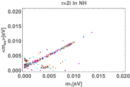
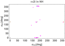
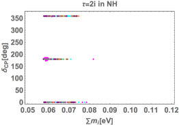
Figure 15: $|\delta\tau|<10^{-15}$ for black, $10^{-15}\leq|\delta\tau|<10^{-12}$ for gray, $10^{-12}\leq|\delta\tau|<10^{-10}$ for purple, $10^{-10}\leq|\delta\tau|<10^{-7}$ for brown, $10^{-7}\leq|\delta\tau|<10^{-5}$ for blue green, $10^{-5}\leq|\delta\tau|<10^{-3}$ for orange, and $10^{-3}\leq|\delta\tau|<10^{-1}$ for magenta.

In Fig. 15, we show the several figures in terms of deviation from $\tau=2i$ in the same case of Fig. 5, where the color legends are the same as the one in Fig. 6. The up-left one is the same as the case of up-right one in Fig. 14. The up-right one is the same as the case of down-left one in Fig. 14. The down-left one is the same as the case of down-right one in Fig. 14. These figures suggest us that size of deviation almost run the whole ranges that are allowed by the neutrino oscillation data.

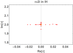
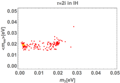
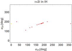
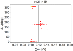
Figure 16: Each of color represents ${\rm blue}\leq 1\sigma$, $1\sigma<{\rm green}\leq 2\sigma$, $2\sigma<{\rm yellow}\leq 3\sigma$, $3\sigma<{\rm red}\leq 5\sigma$.

In Fig. 16, we show our several allowed regions on $\tau$ at nearby $\tau=2i$ in case of IH, where color legends are the same as the one of Fig. 5. Therefore, we have found only the allowed region of $2\sigma-5\sigma$. The up-left one represents the allowed region of the imaginary part of $\tau$ in terms of the real part of $\tau$. The up-right one demonstrates the allowed region of neutrinoless double beta decay $\langle m_{ee}\rangle$ in terms of the lightest active neutrino mass $m_{3}$. We find the allowed regions as follows: 0 eV$\leq m_{3}\leq$0.03 eV and 0.014 eV$\leq\langle m_{ee}\rangle\leq$0.04 eV up to $5\sigma$, but the allowed regions are localized at nearby small masses at yellow plots. The down-left one shows the allowed region of Majorana phases $\alpha_{21}$ and $\alpha_{31}$. $\alpha_{21}$ is allowed by $100^{\circ}$ to $200^{\circ}$, while $\alpha_{31}$ is wider region than $\alpha_{21}$. However the allowed regions are localized at nearby $\alpha_{21}=180^{\circ}$ and $\alpha_{31}=0^{\circ}$ at yellow plots. The down-right one depicts the allowed region of Dirac phase $\delta_{\text{CP}}$ in terms of the sum of neutrino masses $\sum m_{i}$. The vertical line is the upper bound on cosmological constraint. $\delta_{\rm CP}$ is allowed at the points $0^{\circ}$ and $180^{\circ}$. On the other hand, almost half the points of $\sum m_{i}$ would be ruled out by the cosmological bound. Therefore, we would predict a narrow range of $0.1$eV $\leq\sum m_{i}\leq 0.12$ eV that is almost the same as the one in case of $\tau=i$.

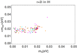
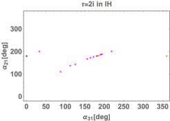
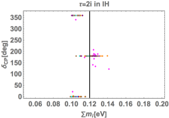
Figure 17: $|\delta\tau|<10^{-15}$ for black, $10^{-15}\leq|\delta\tau|<10^{-12}$ for gray, $10^{-12}\leq|\delta\tau|<10^{-10}$ for purple, $10^{-10}\leq|\delta\tau|<10^{-7}$ for brown, $10^{-7}\leq|\delta\tau|<10^{-5}$ for blue green, $10^{-5}\leq|\delta\tau|<10^{-3}$ for orange, and $10^{-3}\leq|\delta\tau|<10^{-1}$ for magenta.

In Fig. 17, we show the several figures in terms of deviation from $\tau=2i$ in the same case of Fig. 5, where the color legends are the same as the one in Fig. 8. The up-left one is the same as the case of up-right one in Fig. 16. The up-right one is the same as the case of down-left one in Fig. 16. The down-left one is the same as the case of down-right one in Fig. 16. These figures suggest us that size of deviation almost run the whole ranges that are allowed by the neutrino oscillation data.

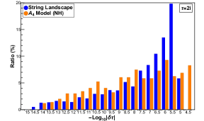
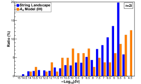
Figure 18: Ratios of the string landscape in Fig. 4 and the $A_{4}$ model within $5\sigma$, where the ratios are defined as those of the number of solutions in a corresponding range of $-{\rm Log}_{10}|\delta\tau|$ to the number of whole solutions. We present the NH and the IH in the left and right panels, respectively.

In a similar to $\tau\simeq i$, we plot ratios of the number of solutions in a corresponding range of $-{\rm Log}_{10}|\delta\tau|$ to the number of whole solutions for both the string landscape in Fig. 2 and the $A_{4}$ model within $5\sigma$ in Fig. 18. It indicates both the distributions of $A_{4}$ model with NH and the moduli fields in the string landscape peak around $|\delta\tau|={\cal O}(10^{-5})$, but such a signal will not be found in the IH case.

Here, we summarize our results where $\tau=\omega$ does not favor a theoretical point of view from the string landscape. Thus, we focus on $\tau=i$ and $\tau=2i$ only. In the case of $\tau=i$ with NH, there is an intriguing tendency that the allowed region of smaller $\chi$ square is localized at smaller $\sum m_{i}$ that is within the cosmological bound. Another feature is that the best fit value of Dirac CP phase $\sim 195^{\circ}$ would be reproduced when we allow up to $5\sigma$ interval. It implies that smaller deviations $|\delta\tau|$ tend to be localized at nearby their smaller masses. In the case of $\tau=i$ with IH, There are two correlations between them; one is a linear line, and another is a slightly curved one. The solutions tend to be localized at nearby smaller mass of $m_{3}$ with $\langle m_{ee}\rangle=0.015,\ 0.05$ eV. A large part of $\sum m_{i}$ would be ruled out by the cosmological bound. Therefore, we would predict a narrow range of $0.1~{}{\rm eV}\leq\sum m_{i}\leq 0.12~{}{\rm eV}$. It implies that smaller deviations $|\delta\tau|$ tend to be localized at nearby their smaller masses $m_{3}$. The smaller deviation would be favored in the point of view of the bound on the cosmological constraint. Both the distributions of $A_{4}$ model with NH and the moduli fields in the string landscape peak around $|\delta\tau|={\cal O}(10^{-5})$, but such a signal is not found. In the case of $\tau=2i$ with NH, the smaller $\chi$ square denoted in blue is closest to the fixed point of $\tau=2i$, which would be a good tendency. We find the allowed regions 0 eV$\leq m_{1}\leq$0.014 eV, and 0 eV$\leq\langle m_{ee}\rangle\leq$0.013 eV. The whole allowed region of $\sum m_{i}$ is totally within the bound on cosmological constraint; 0.058 eV$\leq\sum m_{i}\leq$ 0.082 eV. The size of the deviation from $\tau=2i$ almost runs the whole ranges that are allowed by the neutrino oscillation data. In the case of $\tau=2i$ with IH, we find the allowed regions as follows: 0 eV$\leq m_{3}\leq$0.03 eV and 0.014 eV$\leq\langle m_{ee}\rangle\leq$0.04 eV up to $5\sigma$, but the allowed regions are localized at nearby small masses at yellow plots. $\alpha_{21}$ is allowed by $100^{\circ}$ to $200^{\circ}$, while $\alpha_{31}$ is wider region than $\alpha_{21}$. Almost half the points of $\sum m_{i}$ would be ruled out by the cosmological bound. Therefore, we would predict a narrow range of $0.1$eV $\leq\sum m_{i}\leq 0.12$ eV that is almost the same as the one in the case of $\tau=i$. The size of the deviation from $\tau=2i$ almost runs the whole ranges that are allowed by the neutrino oscillation data. Both the distributions of $A_{4}$ model with NH and moduli fields in the string landscape peak around $|\delta\tau|={\cal O}(10^{-5})$, but such a signal is not found in the IH.

4 Conclusions

The residual flavor symmetries appearing in fixed points of $PSL(2,\mathbb{Z})$ moduli space are employed in a wide variety of modular flavor models, but a small departure of the modulus from fixed points is required to realize the observed masses and mixing angles of quarks/leptons and CP-breaking effects in the bottom-up modular invariant theories. In this paper, we have explicitly demonstrated the breaking of residual flavor symmetry from the top-down approach.

Following Ref. Ishiguro:2020nuf , we have studied the moduli stabilization in the context of Type IIB string theory on $T^{6}/(\mathbb{Z}_{2}\times\mathbb{Z}_{2}^{\prime})$ orientifold. In Type IIB flux compactifications, it was known that $\mathbb{Z}_{2}$ and $\mathbb{Z}_{3}$ fixed points on the fundamental domain of the complex structure modulus space are statistically favored in the finite number of vacua. However, the volume moduli have not been stabilized yet, and a present stage of acceleration of the Universe should be realized. In this respect, we have incorporated non-perturbative corrections to the superpotential as well as uplifting sources to stabilize the volume moduli at the dS vacua. These sources naturally shift the value of $\tau$ from fixed points by a small amount. We find that the deviations of $\tau$ from fixed points $\langle\tau\rangle=i,w,2i$ are statistically favored at $|\delta\tau|\simeq 10^{-5}$ and the CP symmetry $\tau\rightarrow-\bar{\tau}$ is broken in a generic choice of background fluxes. Since the SUSY is broken by the existence of uplifting source, the typical SUSY-breaking scale, i.e., the gravitino mass, is estimated as of ${\cal O}(10^{13})$ GeV at the small departure $|\delta\tau|\simeq 10^{-5}$. In this way, the top-down approach restricts ourselves to the specific value of the modulus $\tau$ as well as the SUSY-breaking scale.

To illustrate phenomenological implications, we analyze the concrete $A_{4}$ modular flavor model with an emphasis on the lepton sector. Under charge assignments for the lepton and Higgs sectors in Tab. 1, we have presented several predictions in the vicinity of three fixed points by a global $\chi^{2}$ analysis in both the normal and inverted hierarchies of neutrinos. It turns out that there exist many phenomenologically promising models around $\langle\tau\rangle=i$ with the normal hierarchy, whose number is compared with that of the string landscape in Fig. 9. It implies similar distributions for string and $A_{4}$ models with respect to $\delta\tau$. Furthermore, there is an intriguing tendency that allowed region of smaller $\chi$ square is localized at smaller $\sum m_{i}$ that is within the cosmological bound.

Before closing our paper, it is worthwhile mentioning the quasi-stable DM candidate due to the tiny deviation from the fixed points in $\tau=i,\ 2i$. In Ref. Kobayashi:2021ajl , especially, DM and neutrino oscillation data can simultaneously be explained at $\tau=i$ where DM is a Majorana heavy fermion with modular weight $-2$. In this set up , DM decays into leptons and Higgses via a Dirac term. Assuming order one free parameter and the DM mass ($m_{X}$) is much heavier than the leptons and Higgses, we estimate its lifetime ($\tau_{X}$) as follows:

$$\tau_{X}\simeq 1.32\times 10^{-25}\times\left|Y^{(6)}_{1}\right|^{-2}\left(\frac{1\ {\rm TeV}}{m_{X}}\right){\rm sec}.$$ (4.1)

When $m_{X}=1$ TeV, the upper limit of $\left|Y^{(6)}_{1}\right|$ be less than the order $10^{-21}$ in order $X$ to be a quasi-stable DM imposing $10^{17}{\rm sec}\lesssim\tau_{X}$. Here, $10^{17}$ sec is the age of the Universe. This constraint is equivalent to $|\delta\tau|\lesssim 5.57\times 10^{-9}$ that is within our valid parameter space.

Appendix A $A_{4}$ modular forms

Note that the modulus-dependent modular forms are constructed by the weight 2 modular form,

$$Y_{\bf 3}^{(2)}=\begin{pmatrix}Y_{1}\\ Y_{2}\\ Y_{3}\\ \end{pmatrix},$$ (A.1)

with

$$Y_{1}(\tau) =\frac{i}{2\pi}\left(\frac{\eta^{\prime}(\tau/3)}{\eta(\tau/3)}+\frac{\eta^{\prime}((\tau+1)/3)}{\eta((\tau+1)/3)}+\frac{\eta^{\prime}((\tau+2)/3)}{\eta((\tau+2)/3)}-\frac{27\eta^{\prime}(3\tau)}{\eta(3\tau)}\right),$$ (A.2)

$$Y_{2}(\tau) =\frac{-i}{\pi}\left(\frac{\eta^{\prime}(\tau/3)}{\eta(\tau/3)}+\omega^{2}\frac{\eta^{\prime}((\tau+1)/3)}{\eta((\tau+1)/3)}+\omega\frac{\eta^{\prime}((\tau+2)/3)}{\eta((\tau+2)/3)}\right),$$ (A.3)

$$Y_{3}(\tau) =\frac{-i}{\pi}\left(\frac{\eta^{\prime}(\tau/3)}{\eta(\tau/3)}+\omega\frac{\eta^{\prime}((\tau+1)/3)}{\eta((\tau+1)/3)}+\omega^{2}\frac{\eta^{\prime}((\tau+2)/3)}{\eta((\tau+2)/3)}\right)\,,$$ (A.4)

where $\eta(\tau)$ denotes the Dedekind eta-function and $\omega=e^{2\pi i/3}$. Recalling that the other modular forms are constructed by tensor products of $Y_{\bf 3}^{(2)}$, we list the modular forms used in our analysis:

$${Y^{\rm(4)}_{\bf 3}}(\tau)=\begin{pmatrix}Y_{1}^{2}-Y_{2}Y_{3}\\ Y_{3}^{2}-Y_{1}Y_{2}\\ Y_{2}^{2}-Y_{1}Y_{3}\end{pmatrix}\,,$$

$$Y_{\bf 1}^{(4)}=Y_{1}^{2}+2Y_{2}Y_{3}\,,\qquad\qquad Y_{\bf 1^{\prime}}^{(4)}=Y_{3}^{2}+2Y_{1}Y_{2}\,.$$

$${Y^{\rm(6)}_{\bf 3}}(\tau)=Y_{\bf 1}^{(4)}{Y^{\rm(2)}_{\bf 3}}(\tau)=(Y_{1}^{2}+2Y_{2}Y_{3})\begin{pmatrix}Y_{1}\\ Y_{2}\\ Y_{3}\end{pmatrix}\,,$$

$${Y^{\rm(6)}_{\bf 3^{\prime}}}(\tau)=Y_{\bf 1^{\prime}}^{(4)}{Y^{\rm(2)}_{\bf 3}}(\tau)=(Y_{3}^{2}+2Y_{1}Y_{2})\begin{pmatrix}Y_{3}\\ Y_{1}\\ Y_{2}\end{pmatrix}\,.$$ (A.5)

References

- (1) R. de Adelhart Toorop, F. Feruglio and C. Hagedorn, Finite Modular Groups and Lepton Mixing, Nucl. Phys. B 858 (2012) 437 [1112.1340].
- (2) S. Ferrara, .D. Lust and S. Theisen, Target Space Modular Invariance and Low-Energy Couplings in Orbifold Compactifications, Phys. Lett. B 233 (1989) 147.
- (3) W. Lerche, D. Lust and N.P. Warner, Duality Symmetries in Landau-ginzburg Models, Phys. Lett. B 231 (1989) 417.
- (4) J. Lauer, J. Mas and H.P. Nilles, Twisted sector representations of discrete background symmetries for two-dimensional orbifolds, Nucl. Phys. B 351 (1991) 353.
- (5) A. Baur, H.P. Nilles, A. Trautner and P.K.S. Vaudrevange, Unification of Flavor, CP, and Modular Symmetries, Phys. Lett. B 795 (2019) 7 [1901.03251].
- (6) A. Baur, H.P. Nilles, A. Trautner and P.K.S. Vaudrevange, A String Theory of Flavor and , Nucl. Phys. B 947 (2019) 114737 [1908.00805].
- (7) T. Kobayashi, S. Nagamoto, S. Takada, S. Tamba and T.H. Tatsuishi, Modular symmetry and non-Abelian discrete flavor symmetries in string compactification, Phys. Rev. D 97 (2018) 116002 [1804.06644].
- (8) T. Kobayashi and S. Tamba, Modular forms of finite modular subgroups from magnetized D-brane models, Phys. Rev. D 99 (2019) 046001 [1811.11384].
- (9) H. Ohki, S. Uemura and R. Watanabe, Modular flavor symmetry on a magnetized torus, Phys. Rev. D 102 (2020) 085008 [2003.04174].
- (10) S. Kikuchi, T. Kobayashi, S. Takada, T.H. Tatsuishi and H. Uchida, Revisiting modular symmetry in magnetized torus and orbifold compactifications, Phys. Rev. D 102 (2020) 105010 [2005.12642].
- (11) S. Kikuchi, T. Kobayashi, H. Otsuka, S. Takada and H. Uchida, Modular symmetry by orbifolding magnetized : realization of double cover of , JHEP 11 (2020) 101 [2007.06188].
- (12) S. Kikuchi, T. Kobayashi and H. Uchida, Modular flavor symmetries of three-generation modes on magnetized toroidal orbifolds, Phys. Rev. D 104 (2021) 065008 [2101.00826].
- (13) Y. Almumin, M.-C. Chen, V. Knapp-Pérez, S. Ramos-Sánchez, M. Ratz and S. Shukla, Metaplectic Flavor Symmetries from Magnetized Tori, JHEP 05 (2021) 078 [2102.11286].
- (14) A. Baur, M. Kade, H.P. Nilles, S. Ramos-Sanchez and P.K.S. Vaudrevange, Siegel modular flavor group and CP from string theory, Phys. Lett. B 816 (2021) 136176 [2012.09586].
- (15) A. Strominger, SPECIAL GEOMETRY, Commun. Math. Phys. 133 (1990) 163.
- (16) P. Candelas and X. de la Ossa, Moduli Space of Calabi-Yau Manifolds, Nucl. Phys. B 355 (1991) 455.
- (17) K. Ishiguro, T. Kobayashi and H. Otsuka, Spontaneous CP violation and symplectic modular symmetry in Calabi-Yau compactifications, Nucl. Phys. B 973 (2021) 115598 [2010.10782].
- (18) K. Ishiguro, T. Kobayashi and H. Otsuka, Symplectic modular symmetry in heterotic string vacua: flavor, CP, and R-symmetries, JHEP 01 (2022) 020 [2107.00487].
- (19) F. Feruglio, Are neutrino masses modular forms?, in From My Vast Repertoire …: Guido Altarelli’s Legacy, A. Levy, S. Forte and G. Ridolfi, eds., pp. 227–266 (2019), DOI [1706.08749].
- (20) T. Kobayashi, K. Tanaka and T.H. Tatsuishi, Neutrino mixing from finite modular groups, Phys. Rev. D 98 (2018) 016004 [1803.10391].
- (21) J.T. Penedo and S.T. Petcov, Lepton Masses and Mixing from Modular Symmetry, Nucl. Phys. B 939 (2019) 292 [1806.11040].
- (22) P.P. Novichkov, J.T. Penedo, S.T. Petcov and A.V. Titov, Modular A5 symmetry for flavour model building, JHEP 04 (2019) 174 [1812.02158].
- (23) G.-J. Ding, S.F. King and X.-G. Liu, Neutrino mass and mixing with modular symmetry, Phys. Rev. D 100 (2019) 115005 [1903.12588].
- (24) X.-G. Liu and G.-J. Ding, Neutrino Masses and Mixing from Double Covering of Finite Modular Groups, JHEP 08 (2019) 134 [1907.01488].
- (25) P. Chen, G.-J. Ding, J.-N. Lu and J.W.F. Valle, Predictions from warped flavor dynamics based on the family group, Phys. Rev. D 102 (2020) 095014 [2003.02734].
- (26) P.P. Novichkov, J.T. Penedo and S.T. Petcov, Double cover of modular for flavour model building, Nucl. Phys. B 963 (2021) 115301 [2006.03058].
- (27) X.-G. Liu, C.-Y. Yao and G.-J. Ding, Modular invariant quark and lepton models in double covering of modular group, Phys. Rev. D 103 (2021) 056013 [2006.10722].
- (28) X. Wang, B. Yu and S. Zhou, Double covering of the modular group and lepton flavor mixing in the minimal seesaw model, Phys. Rev. D 103 (2021) 076005 [2010.10159].
- (29) C.-Y. Yao, X.-G. Liu and G.-J. Ding, Fermion masses and mixing from the double cover and metaplectic cover of the modular group, Phys. Rev. D 103 (2021) 095013 [2011.03501].
- (30) G.-J. Ding, S.F. King, C.-C. Li and Y.-L. Zhou, Modular Invariant Models of Leptons at Level 7, JHEP 08 (2020) 164 [2004.12662].
- (31) T. Kobayashi, H. Otsuka, M. Tanimoto and K. Yamamoto, Modular symmetry in the SMEFT, Phys. Rev. D 105 (2022) 055022 [2112.00493].
- (32) T. Kobayashi, H. Otsuka, M. Tanimoto and K. Yamamoto, Lepton flavor violation, lepton and electron EDM in the modular symmetry, 2204.12325.
- (33) T. Kobayashi and H. Otsuka, On stringy origin of minimal flavor violation, Eur. Phys. J. C 82 (2022) 25 [2108.02700].
- (34) P.P. Novichkov, J.T. Penedo, S.T. Petcov and A.V. Titov, Generalised CP Symmetry in Modular-Invariant Models of Flavour, JHEP 07 (2019) 165 [1905.11970].
- (35) P.P. Novichkov, J.T. Penedo, S.T. Petcov and A.V. Titov, Modular S4 models of lepton masses and mixing, JHEP 04 (2019) 005 [1811.04933].
- (36) P.P. Novichkov, S.T. Petcov and M. Tanimoto, Trimaximal Neutrino Mixing from Modular A4 Invariance with Residual Symmetries, Phys. Lett. B 793 (2019) 247 [1812.11289].
- (37) G.-J. Ding, S.F. King, X.-G. Liu and J.-N. Lu, Modular S4 and A4 symmetries and their fixed points: new predictive examples of lepton mixing, JHEP 12 (2019) 030 [1910.03460].
- (38) H. Okada and M. Tanimoto, Towards unification of quark and lepton flavors in modular invariance, Eur. Phys. J. C 81 (2021) 52 [1905.13421].
- (39) S.F. King and Y.-L. Zhou, Trimaximal TM1 mixing with two modular groups, Phys. Rev. D 101 (2020) 015001 [1908.02770].
- (40) H. Okada and M. Tanimoto, Quark and lepton flavors with common modulus in modular symmetry, 2005.00775.
- (41) H. Okada and M. Tanimoto, Modular invariant flavor model of and hierarchical structures at nearby fixed points, Phys. Rev. D 103 (2021) 015005 [2009.14242].
- (42) H. Okada and M. Tanimoto, Spontaneous CP violation by modulus in model of lepton flavors, JHEP 03 (2021) 010 [2012.01688].
- (43) F. Feruglio, V. Gherardi, A. Romanino and A. Titov, Modular invariant dynamics and fermion mass hierarchies around , JHEP 05 (2021) 242 [2101.08718].
- (44) T. Kobayashi, H. Okada and Y. Orikasa, Dark matter stability at fixed points in a modular symmetry, 2111.05674.
- (45) T. Kobayashi, Y. Shimizu, K. Takagi, M. Tanimoto and T.H. Tatsuishi, lepton flavor model and modulus stabilization from modular symmetry, Phys. Rev. D 100 (2019) 115045 [1909.05139].
- (46) T. Kobayashi, Y. Shimizu, K. Takagi, M. Tanimoto, T.H. Tatsuishi and H. Uchida, violation in modular invariant flavor models, Phys. Rev. D 101 (2020) 055046 [1910.11553].
- (47) T. Kobayashi and H. Otsuka, Challenge for spontaneous violation in Type IIB orientifolds with fluxes, Phys. Rev. D 102 (2020) 026004 [2004.04518].
- (48) K. Ishiguro, T. Kobayashi and H. Otsuka, Landscape of Modular Symmetric Flavor Models, JHEP 03 (2021) 161 [2011.09154].
- (49) P.P. Novichkov, J.T. Penedo and S.T. Petcov, Modular Flavour Symmetries and Modulus Stabilisation, 2201.02020.
- (50) T. Kobayashi and H. Otsuka, Classification of discrete modular symmetries in Type IIB flux vacua, Phys. Rev. D 101 (2020) 106017 [2001.07972].
- (51) O. DeWolfe, A. Giryavets, S. Kachru and W. Taylor, Enumerating flux vacua with enhanced symmetries, JHEP 02 (2005) 037 [hep-th/0411061].
- (52) S. Kachru, R. Kallosh, A.D. Linde and S.P. Trivedi, De Sitter vacua in string theory, Phys. Rev. D 68 (2003) 046005 [hep-th/0301240].
- (53) S. Kikuchi, T. Kobayashi, K. Nasu, H. Otsuka, S. Takada and H. Uchida, Modular symmetry of soft supersymmetry breaking terms, 2203.14667.
- (54) X. Du and F. Wang, SUSY breaking constraints on modular flavor invariant SU(5) GUT model, JHEP 02 (2021) 221 [2012.01397].
- (55) T. Kobayashi, T. Shimomura and M. Tanimoto, Soft supersymmetry breaking terms and lepton flavor violations in modular flavor models, Phys. Lett. B 819 (2021) 136452 [2102.10425].
- (56) H. Otsuka and H. Okada, Radiative neutrino masses from modular symmetry and supersymmetry breaking, 2202.10089.
- (57) S. Gukov, C. Vafa and E. Witten, CFT’s from Calabi-Yau four folds, Nucl. Phys. B 584 (2000) 69 [hep-th/9906070].
- (58) P. Betzler and E. Plauschinn, Type IIB flux vacua and tadpole cancellation, Fortsch. Phys. 67 (2019) 1900065 [1905.08823].
- (59) P. Candelas, E. Perevalov and G. Rajesh, Toric geometry and enhanced gauge symmetry of F theory / heterotic vacua, Nucl. Phys. B 507 (1997) 445 [hep-th/9704097].
- (60) W. Taylor and Y.-N. Wang, The F-theory geometry with most flux vacua, JHEP 12 (2015) 164 [1511.03209].
- (61) M. Demirtas, M. Kim, L. Mcallister and J. Moritz, Vacua with Small Flux Superpotential, Phys. Rev. Lett. 124 (2020) 211603 [1912.10047].
- (62) Y. Honma and H. Otsuka, Small flux superpotential in F-theory compactifications, Phys. Rev. D 103 (2021) 126022 [2103.03003].
- (63) H. Abe, T. Higaki and T. Kobayashi, Remark on integrating out heavy moduli in flux compactification, Phys. Rev. D 74 (2006) 045012 [hep-th/0606095].
- (64) KamLAND-Zen collaboration, Search for Majorana Neutrinos near the Inverted Mass Hierarchy Region with KamLAND-Zen, Phys. Rev. Lett. 117 (2016) 082503 [1605.02889].
- (65) I. Esteban, M.C. Gonzalez-Garcia, M. Maltoni, T. Schwetz and A. Zhou, The fate of hints: updated global analysis of three-flavor neutrino oscillations, JHEP 09 (2020) 178 [2007.14792].
- (66) F. Björkeroth, F.J. de Anda, I. de Medeiros Varzielas and S.F. King, Towards a complete A SU(5) SUSY GUT, JHEP 06 (2015) 141 [1503.03306].
- (67) I. Esteban, M.C. Gonzalez-Garcia, A. Hernandez-Cabezudo, M. Maltoni and T. Schwetz, Global analysis of three-flavour neutrino oscillations: synergies and tensions in the determination of , , and the mass ordering, JHEP 01 (2019) 106 [1811.05487].
- (68) Planck collaboration, Planck 2018 results. VI. Cosmological parameters, Astron. Astrophys. 641 (2020) A6 [1807.06209].