Limit results for distributed estimation of invariant subspaces in multiple networks inference and PCA

Abstract

We study the problem of distributed estimation of the leading singular vectors for a collection of matrices with shared invariant subspaces. In particular we consider an algorithm that first estimates the projection matrices corresponding to the leading singular vectors for each individual matrix, then computes the average of the projection matrices, and finally returns the leading eigenvectors of the sample averages. We show that the algorithm, when applied to (1) parameters estimation for a collection of independent edge random graphs with shared singular vectors but possibly heterogeneous edge probabilities or (2) distributed PCA for independent sub-Gaussian random vectors with spiked covariance structure, yields estimates whose row-wise fluctuations are normally distributed around the rows of the true singular vectors. Leveraging these results we also consider a two-sample test for the null hypothesis that a pair of random graphs have the same edge probabilities and we present a test statistic whose limiting distribution converges to a central (resp. non-central) $\chi^{2}$ under the null (resp. local alternative) hypothesis.

and

1 Introduction

Distributed estimation, also known as divide-and-conquer or aggregated inference, is used in numerous methodological applications including regression [aggregated_inference_huo, ridge_regression_dobriban], integrative data analysis [jive, feng2018angle, hector], multiple networks inference [arroyo2019inference], distributed PCA and image populations analysis [population_svd, sagonas2017robust, tang2021integrated, fan2019distributed, chen2021distributed], and is also a key component underlying federated learning [federated_survey]. These types of procedures are particularly important for analyzing large-scale datasets that are scattered across multiple organizations and/or computing nodes where both the computational complexities and communication costs (as well as possibly privacy constraints) prevent the transfer of all the raw data to a single location.

In this paper, we focus on distributed estimation of the leading singular vectors for a collection of matrices with shared invariant subspaces, and we analyze an algorithm that first estimates the projection matrices corresponding to the leading singular vectors for each individual matrix, then computes the average of the projection matrices, and finally returns the leading eigenvectors of the sample averages. One widely studied example of this problem is distributed PCA in which there are $N$ independent $D$-dimensional sub-Gaussian random vectors $\{X_{j}\}_{j=1}^{N}$ with common covariance matrix $\bm{\Sigma}$ scattered across $m$ computing nodes, and the goal is to find the leading eigenspace of $\bm{\Sigma}$. Letting $\mathbf{X}^{(i)}$ be the $D\times n_{i}$ matrix whose columns are the subsample of $\{X_{j}\}_{i=1}^{N}$ stored in node $i$, the authors of [fan2019distributed] analyze a procedure where each node $i\in\{1,2,\dots,m\}$ first computes the $D\times d$ matrix $\hat{\mathbf{U}}^{(i)}$ whose columns are the leading left singular vectors of $\mathbf{X}^{(i)}$. These $\{\hat{\mathbf{U}}^{(i)}\}$ are then sent to a central computing node which outputs the leading eigenvectors of $m^{-1}\sum_{i=1}^{m}\hat{\mathbf{U}}^{(i)}(\hat{\mathbf{U}}^{(i)})^{\top}$ as the estimate for the principal components of $\bm{\Sigma}$. An almost identical procedure is also used for simultaneous dimension reduction of high-dimensional images $\{\mathbf{Y}_{i}\}_{i=1}^{m}$, i.e., each $\mathbf{Y}_{i}$ is a $F\times T$ matrix whose entries are measurements recorded for various frequencies and various times, and the goal is to find a “population value decomposition” of each $\mathbf{Y}_{i}$ as $\mathbf{Y}_{i}\approx\mathbf{P}\mathbf{V}_{i}\mathbf{D}$. Here $\mathbf{P}$ and $\mathbf{D}$ are $F\times A$ and $A\times T$ matrices (with $A\ll\min\{F,T\}$) representing population frames of references, and $\{\mathbf{V}_{i}\}$ are the subject-level features; see [population_svd] for more details. The procedure in [fan2019distributed, population_svd] can also be used for estimating the invariant leading eigenspace of multiple adjacency matrices $\{\mathbf{A}^{(i)}\}$ generated from the COSIE model [arroyo2019inference] where $\mathbb{E}[\mathbf{A}^{(i)}]=\mathbf{U}\mathbf{R}^{(i)}\mathbf{U}^{\top}$ and $\mathbf{U}$ (resp. $\{\mathbf{R}^{(i)}\}$) represents the common structure (resp. possibly heterogeneity) across $\{\mathbf{A}^{(i)}\}$. As a final example, a typical setting for integrative data analysis assumes that there is a collection of data matrices $\{\mathbf{X}^{(i)}\}$ from multiple disparate sources and the goal is to decompose each $\mathbf{X}^{(i)}$ as $\mathbf{X}^{(i)}=\mathbf{J}^{(i)}+\mathbf{I}^{(i)}+\mathbf{N}^{(i)}$, where $\{\mathbf{J}^{(i)}\}$ share a common row space $\mathbf{J}_{*}$ which captures the joint structure among all $\{\mathbf{X}^{(i)}\}$, $\{\mathbf{I}^{(i)}\}$ represent the individual structure in each $\mathbf{X}^{(i)}$, and $\{\mathbf{N}^{(i)}\}$ are noise matrices. Several algorithms, such as aJIVE and robust aJIVE [feng2018angle, ponzi2021rajive], compute an estimate $\hat{\mathbf{J}}_{*}$ of $\mathbf{J}_{*}$ by aggregating the leading (right) singular vectors $\{\hat{\mathbf{U}}^{(i)}\}$ of $\{\mathbf{X}^{(i)}\}$ and then estimate each individual $\mathbf{I}^{(i)}$ by projecting $\mathbf{X}^{(i)}$ onto the orthogonal complement of the $\hat{\mathbf{J}}_{*}$.

1.1 Outline of results

Despite the wide applicability of the distributed estimators for invariant subspaces described above, their theoretical results are still somewhat limited. For example, the papers that proposed the aJIVE/rAJIVE procedures [feng2018angle, ponzi2021rajive] and the PVD [population_svd] do not consider any specific noise models and thus also do not present explicit error bounds for the estimates. Similarly, in the context of the COSIE model and distributed PCA, [arroyo2019inference] and [population_svd, tang2021integrated, fan2019distributed, chen2021distributed], only provide Frobenius norm upper bounds between $\hat{\mathbf{U}}$ and $\mathbf{U}$. In this paper we present a general framework for analyzing these types of estimators, with special emphasis on uniform $\ell_{2\to\infty}$ error bounds and normal approximations for the row-wise fluctuations of $\hat{\mathbf{U}}$ around $\mathbf{U}$. A key contribution of our paper is summarized in the following result (see Section 1.2 for a description of the notations used here).

Theorem 1.

Let $\{\mathbf{U}^{(i)}=[\mathbf{U}_{c}|\mathbf{U}_{s}^{(i)}]\}_{i=1}^{m}$ be a collection of matrices of size $n_{\ell}\times d_{i}$, with $\mathbf{U}^{(i)\top}\mathbf{U}^{(i)}=\mathbf{I}$ for all $i\in[m]$. Let $d_{0}$ denote the number of columns of $\mathbf{U}_{c}$ and define $\bm{\Pi}_{s}=m^{-1}\sum_{i=1}^{m}\mathbf{U}^{(i)}\mathbf{U}^{(i)\top}$. Now let $\{\mathbf{A}^{(i)}\}_{i=1}^{m}$ be any arbitrary collection of $n_{\ell}\times n_{r}^{(i)}$ matrices and denote $\hat{\mathbf{U}}^{(i)}$ as the matrix whose columns are the leading $d_{i}$ left singular vectors of each $\mathbf{A}^{(i)}$. Suppose that for each $i\in[m]$ one has the expansion

$$\hat{\mathbf{U}}^{(i)}\mathbf{W}_{\mathbf{U}}^{(i)}-\mathbf{U}^{(i)}=\mathbf{T}_{0}^{(i)}+\mathbf{T}^{(i)},$$

where $\mathbf{W}^{(i)}_{\mathbf{U}}$ is a orthogonal matrix and $\mathbf{T}_{0}^{(i)},\mathbf{T}^{(i)}$ satisfy

$$\max_{i\in[m]}\Bigl{(}2\|\mathbf{T}_{0}^{(i)}\|+2\|\mathbf{T}^{(i)}\|+\|\mathbf{T}_{0}^{(i)}+\mathbf{T}^{(i)}\|^{2}\Bigr{)}\leq c(1-\|\bm{\Pi}_{s}\|)$$ (1.1)

for some constant $c<\frac{1}{2}$. Define the quantities

$$\begin{split}\zeta_{\mathbf{U}}=\max_{i\in[m]}\|\mathbf{U}^{(i)}\|_{2\to\infty},\quad\epsilon_{\star}=\max_{i\in[m]}\|\mathbf{U}^{(i)\top}\mathbf{T}_{0}^{(i)}\|,\\ \epsilon_{\mathbf{T}_{0}}=\max_{i\in[m]}\|\mathbf{T}_{0}^{(i)}\|,\quad\zeta_{\mathbf{T}_{0}}=\max_{i\in[m]}\|\mathbf{T}_{0}^{(i)}\|_{2\to\infty},\\ \epsilon_{\mathbf{T}}=\max_{i\in[m]}\|\mathbf{T}^{(i)}\|,\quad\zeta_{\mathbf{T}}=\max_{i\in[m]}\|\mathbf{T}^{(i)}\|_{2\to\infty}.\end{split}$$ (1.2)

Now let $\hat{\mathbf{U}}_{c}$ be the matrix whose columns are the $d_{0}$ leading eigenvectors of $m^{-1}\sum_{i=1}^{m}\hat{\mathbf{U}}^{(i)}\hat{\mathbf{U}}^{(i)\top}$ and let $\mathbf{W}_{\mathbf{U}_{c}}$ be a minimizer of $\|\hat{\mathbf{U}}_{c}\mathbf{O}-\mathbf{U}_{c}\|_{F}$ over all $d_{0}\times d_{0}$ orthogonal matrix $\mathbf{O}$. Then

$$\hat{\mathbf{U}}_{c}\mathbf{W}_{\mathbf{U}_{c}}-\mathbf{U}_{c}=\frac{1}{m}\sum_{i=1}^{m}\mathbf{T}_{0}^{(i)}\mathbf{U}^{(i)\top}\mathbf{U}_{c}+\mathbf{Q}_{\mathbf{U}_{c}},$$ (1.3)

where $\mathbf{Q}_{\mathbf{U}_{c}}$ is a matrix satisfying

$$\|\mathbf{Q}_{\mathbf{U}_{c}}\|\lesssim\epsilon_{\star}+\epsilon_{\mathbf{T}_{0}}^{2}+\epsilon_{\mathbf{T}},$$ (1.4)

$$\|\mathbf{Q}_{\mathbf{U}_{c}}\|_{2\to\infty}\lesssim\zeta_{\mathbf{U}}(\epsilon_{\star}+\epsilon_{\mathbf{T}_{0}}^{2}+\epsilon_{\mathbf{T}})+\zeta_{\mathbf{T}_{0}}(\epsilon_{\star}+\epsilon_{\mathbf{T}_{0}}+\epsilon_{\mathbf{T}})+\zeta_{\mathbf{T}}.$$

Given $\hat{\mathbf{U}}_{c}$, let $\hat{\mathbf{U}}_{s}^{(i)}$ be the matrix whose columns are the $d_{i}-d_{0}$ leading left singular vectors of $(\mathbf{I}-\hat{\mathbf{U}}_{c}\hat{\mathbf{U}}_{c}^{\top})\hat{\mathbf{U}}^{(i)}$ and let $\mathbf{W}^{(i)}_{\mathbf{U}_{s}}$ be a minimizer of $\|\hat{\mathbf{U}}_{s}^{(i)}\mathbf{O}-\mathbf{U}_{s}^{(i)}\|_{F}$ over all orthogonal matrix $\mathbf{O}$. Then for all $i\in[m]$ we have

$$\hat{\mathbf{U}}_{s}^{(i)}\mathbf{W}^{(i)}_{\mathbf{U}_{s}}-\mathbf{U}_{s}^{(i)}=\mathbf{T}_{0}^{(i)}\mathbf{U}^{(i)\top}\mathbf{U}_{s}^{(i)}+\mathbf{Q}_{\mathbf{U}_{s}}^{(i)},$$ (1.5)

where $\mathbf{Q}_{\mathbf{U}_{s}}^{(i)}$ is a matrix satisfying the same upper bounds as those for $\mathbf{Q}_{\mathbf{U}_{c}}$.

Theorem 1 is a deterministic matrix perturbation bound which combines the individual expansions for $\{\hat{\mathbf{U}}^{(i)}\}$ into a single expansion for $\hat{\mathbf{U}}$. The upper bounds for $\mathbf{Q}_{\mathbf{U}_{c}}$ and $\{\mathbf{Q}_{\mathbf{U}_{s}}^{(i)}\}$ in Theorem 1 depend only on $\epsilon_{\star},\epsilon_{\mathbf{T}_{0}},\zeta_{\mathbf{T}_{0}},\epsilon_{\mathbf{T}},\zeta_{\mathbf{T}}$ and $\zeta_{\mathbf{U}}$. While bounds for these quantities can be derived for many different settings, in this paper for conciseness and ease of presentation we analyze these quantities only for the COSIE model and distributed PCA as (1) both problems are widely studied and yet (2) our results are still novel. In particular, the COSIE model is a natural extension of the multi-layer SBM, and although there are a wealth of theoretical results for multi-layer SBMs (see e.g., [paul2020spectral, chen2020global, jing2021community, lei2020bias]), they are mainly based on procedures that first aggregate the individual networks (either through a joint likelihood or by taking a weighted sum of the adjacency matrices) before computing an estimate, and are thus conceptually quite different from the distributed estimators considered in Theorem 1 (where the aggregation is done on the individual estimates); see Section 2.2 for a detailed comparison. Similarly, existing results for distributed PCA [chen2021distributed, charisopoulos2021communication, fan2019distributed, liang2014improved] mainly focus on spectral/Frobenius error bounds for $\mathbf{U}$ and are thus coarser than the row-wise limiting results presented here.

The structure of our paper is as follows. In Section 2 we study parameters estimations for the COSIE model for both undirected networks (where $\mathbf{P}^{(i)}=\mathbf{U}\mathbf{R}^{(i)}\mathbf{U}^{\top}$ as considered in [arroyo2019inference]) and directed networks (where $\mathbf{P}^{(i)}=\mathbf{U}\mathbf{R}^{(i)}\mathbf{V}^{\top}$). We show that the rows of the estimates $\hat{\mathbf{U}}$ and $\hat{\mathbf{V}}$ are normally distributed around the rows of $\mathbf{U}$ and $\mathbf{V}$, respectively, and that for all $i\in[m]$, $\hat{\mathbf{R}}^{(i)}$ also converges to a multivariate normal distribution centered around $\mathbf{R}^{(i)}$ with a specific bias. We then consider two-sample (and multi-sample) testing for the null hypothesis that a collection of graphs from the COSIE model have the same edge probabilities matrices, and leveraging the theoretical results for $\{\hat{\mathbf{R}}^{(i)}\}$, we derive a test statistic whose limiting distribution converges to a central $\chi^{2}$ (resp. non-central $\chi^{2}$) under the null (resp. local alternative) hypothesis. In Section 3 we apply Theorem 1 to the distributed PCA setting, and derive normal approximations for the rows of the leading principal components when the data exhibit a spiked covariance structure. Numerical simulations and experiments on real data are presented in Section 4. Detailed proofs of all stated results are presented in the supplementary material.

1.2 Notations

We summarize some notations used in this paper. For a positive integer $p$, we denote by $[p]$ the set $\{1,\dots,p\}$. For two non-negative sequences $\{a_{n}\}_{n\geq 1}$ and $\{b_{n}\}_{n\geq 1}$, we write $a_{n}\lesssim b_{n}$ ($a_{n}\gtrsim b_{n}$, resp.) if there exists some constant $C>0$ such that $a_{n}\leq Cb_{n}$ ($a_{n}\geq Cb_{n}$, resp.) for all $n\geq 1$, and we write $a_{n}\asymp b_{n}$ if $a_{n}\lesssim b_{n}$ and $a_{n}\gtrsim b_{n}$. The notation $a_{n}\ll b_{n}$ ($a_{n}\gg b_{n}$, resp.) means that there exists some sufficiently small (large, resp.) constant $C>0$ such that $a_{n}\leq Cb_{n}$ ($a_{n}\geq Cb_{n}$, resp.). If $a_{n}/b_{n}$ stays bounded away from $+\infty$, we write $a_{n}=O(b_{n})$ and $b_{n}=\Omega(a_{n})$, and we use the notation $a_{n}=\Theta(b_{n})$ to indicate that $a_{n}=O(b_{n})$ and $a_{n}=\Omega(b_{n})$. If $a_{n}/b_{n}\to 0$, we write $a_{n}=o(b_{n})$ and $b_{n}=\omega(a_{n})$. We say a sequence of events $\mathcal{A}_{n}$ holds with high probability if for any $c>0$ there exists a finite constant $n_{0}$ depending only on $c$ such that $\mathbb{P}(\mathcal{A}_{n})\geq 1-n^{-c}$ for all $n\geq n_{0}$. We write $a_{n}=O_{p}(b_{n})$ (resp. $a_{n}=o_{p}(b_{n})$) to denote that $a_{n}=O(b_{n})$ (resp. $a_{n}=o(b_{n})$) holds with high probability. We denote by $\mathcal{O}_{d}$ the set of $d\times d$ orthogonal matrices. Given a matrix $\mathbf{M}$, we denote its spectral, Frobenius, and infinity norms by $\|\mathbf{M}\|$, $\|\mathbf{M}\|_{F}$, and $\|\mathbf{M}\|_{\infty}$, respectively. We also denote the maximum entry (in modulus) of $\mathbf{M}$ by $\|\mathbf{M}\|_{\max}$ and the $2\to\infty$ norm of $\mathbf{M}$ by

$$\|\mathbf{M}\|_{2\to\infty}=\max_{\|\bm{x}\|=1}\|\mathbf{M}\bm{x}\|_{\infty}=\max_{i}\|m_{i}\|,$$

where $m_{i}$ denote the $i$th row of $\mathbf{M}$, i.e., $\|\mathbf{M}\|_{2\to\infty}$ is the maximum of the $\ell_{2}$ norms of the rows of $\mathbf{M}$. We note that the $2\to\infty$ norm is not sub-multiplicative. However, for any matrices $\mathbf{M}$ and $\mathbf{N}$ of conformal dimensions, we have

$$\|\mathbf{M}\mathbf{N}\|_{2\to\infty}\leq\min\{\|\mathbf{M}\|_{2\to\infty}\times\|\mathbf{N}\|,\|\mathbf{M}\|_{\infty}\times\|\mathbf{N}\|_{2\to\infty}\};$$

see Proposition 6.5 in [cape2019two]. Perturbation bounds using the $2\to\infty$ norm for the eigenvectors and/or singular vectors of a noisily observed matrix norm had recently attracted interests from the statistics community, see e.g., [chen2021spectral, cape2019two, lei2019unified, damle, fan2018eigenvector, abbe2020entrywise] and the references therein.

2 COSIE Model

Inference for multiple networks is an important and nascent research area with applications to diverse scientific fields including neuroscience [bullmore2009complex, battiston2017multilayer, de2017multilayer, kong2021multiplex], economics [schweitzer2009economic, lee2016strength], and social sciences [papalexakis2013more, greene2013producing]. One of the simplest and most widely-studied models for a single network $\mathcal{G}$ is the stochastic blockmodel (SBM) [holland1983stochastic] where each node $v$ of $\mathcal{G}$ is assigned to a block $\tau_{v}\in[d]$ and the edges between pairs of vertices $\{u,v\}$ are independent Bernoulli random variables with success probabilities $\mathbf{B}_{\tau_{u},\tau_{v}}$. Here $d\geq 2$ denotes the number of blocks and $\mathbf{B}$ is a $d\times d$ symmetric matrix with real-valued entries in $[0,1]$ specifying the edge probabilities within and between blocks. A natural generalization of the SBM is the multi-layer SBM [tang2009clustering, kumar2011co, han2015consistent, paul2016consistent, lei2020bias, paul2020spectral] wherein there are a collection of $m$ SBM graphs $\{\mathcal{G}_{1},\dots,\mathcal{G}_{m}\}$ on the same vertex set $\mathcal{V}$ with a common community assignment $\tau\colon\mathcal{V}\mapsto[d]$ but possibly different block probabilities matrices $\{\mathbf{B}^{(i)}\}_{i=1}^{m}$. The single and multi-layer SBMs can be viewed as edge-independent graphs where the edge probabilities matrices have both a low-rank and block constant structure. More specifically let $\{\mathcal{G}_{i}\}$ be a multi-layer SBM and denote by $\mathbf{Z}$ the $|\mathcal{V}|\times d$ matrix with binary entries such that $z_{vk}=1$ if and only if the $v$th vertex is assigned to the $k$th block. Then $\mathbf{P}^{(i)}=\mathbf{Z}\mathbf{B}^{(i)}\mathbf{Z}^{\top}$ is the edge probabilities matrix for each $\mathcal{G}_{i}$, i.e., the edges of $\mathcal{G}_{i}$ are independent Bernoulli random variables with success probabilities given by entries of $\mathbf{P}^{(i)}$.

Another class of model for multiple networks is based on the notion of generalized random dot product graphs (GRDPG) [young2007random, grdpg1]. A graph $\mathcal{G}$ is an instance of a GRDPG if each vertex $v$ is associated with a latent position $X_{v}\in\mathbb{R}^{d}$ and the edges between pairs of vertices $\{u,v\}$ are independent Bernoulli random variables with success probablities $\langle X_{u},X_{v}\rangle$ where $\langle\cdot,\cdot\rangle$ denotes a (generalized) inner product in $\mathbb{R}^{d}$. The edge probabilities matrix of a GRDPG can be written as $\mathbf{P}=\mathbf{U}\mathbf{R}\mathbf{U}^{\top}$ where the rows of $\mathbf{U}$ are the (normalized) latent positions associated with the vertices in $\mathcal{G}$ and $\mathbf{R}$ is a $d\times d$ matrix representing a (generalized) inner product; $\mathbf{P}$ is also low-rank but, in contrast to a SBM, needs not to have any constant block structure. The GRDPG thus includes, as special cases, the SBM and its variants including the degree-corrected, mixed-memberships, and popularity adjusted block models [sengupta_chen, karrer2011stochastic, Airoldi2008]. A natural formulation of the GRDPG for multiple networks $\{\mathcal{G}_{i}\}$ is to assume that each $\mathcal{G}_{i}$ is an edge independent random graph where the edge probabilities are $\mathbf{P}^{(i)}=\mathbf{U}\mathbf{R}^{(i)}\mathbf{U}^{\top}$. The resulting networks share a common latent structure induced by $\mathbf{U}$ but with possibly heterogeneous connectivity patterns across networks as modeled by $\{\mathbf{R}^{(i)}\}$. Examples of the above formulation include the common subspace independent edge graphs (COSIE) model [arroyo2019inference] where $\{\mathbf{R}^{(i)}\}$ are arbitrary invertible matrices and the multiple eigenscaling model [nielsen2018multiple, wang2019joint, draves2020bias] where $\{\mathbf{R}^{(i)}\}$ are diagonal matrices. In this paper we consider a slight variant of the COSIE model that is suitable for directed networks.

Definition 1 (Common subspace independent edge graphs).

Let $\mathbf{U}$ and $\mathbf{V}$ be $n\times d$ matrices with orthonormal columns and let $\mathbf{R}^{(1)},\ldots,\mathbf{R}^{(m)}$ be $d\times d$ matrices such that $u_{s}^{\top}\mathbf{R}^{(i)}v_{t}\in[0,1]$ for all $s,t\in[n]$ and $i\in[m]$. Here $u_{s}$ and $v_{t}$ denote the $s$th and $t$th row of $\mathbf{U}$ and $\mathbf{V}$, respectively. We say that the random adjacency matrices $\mathbf{A}^{(1)},\ldots,\mathbf{A}^{(m)}$ are jointly distributed according to the common subspace independent-edge graph model with parameters $\mathbf{U},\mathbf{V},\mathbf{R}^{(1)},\ldots,\mathbf{R}^{(m)}$ if, for each $i\in[m]$, $\mathbf{A}^{(i)}$ is a $n\times n$ random matrix whose entries $\{\mathbf{A}_{st}^{(i)}\}$ are independent Bernoulli random variables with $\mathbb{P}[\mathbf{A}_{st}^{(i)}=1]=u_{s}^{\top}\mathbf{R}^{(i)}v_{t}$. In other words,

$$\mathbb{P}\big{(}\mathbf{A}^{(i)}\mid\mathbf{U},\mathbf{V},\mathbf{R}^{(i)}\big{)}=\prod_{s\in[n]}\prod_{t\in[n]}\big{(}u_{s}^{\top}\mathbf{R}^{(i)}v_{t}\big{)}^{\mathbf{A}_{st}^{(i)}}\big{(}1-u_{s}^{\top}\mathbf{R}^{(i)}v_{t}\big{)}^{1-\mathbf{A}_{st}^{(i)}}.$$

We write $\left(\mathbf{A}^{(1)},\ldots,\mathbf{A}^{(m)}\right)\sim\operatorname{COSIE}\left(\mathbf{U},\mathbf{V};\mathbf{R}^{(1)},\ldots,\mathbf{R}^{(m)}\right)$ to denote a collection of random graphs generated from the above model, and we write $\mathbf{P}^{(i)}=\mathbf{U}\mathbf{R}^{(i)}\mathbf{V}^{\top}$ to denote the (unobserved) edge probabilities matrix for each graph $\mathbf{A}^{(i)}$. We note that the COSIE model in [arroyo2019inference] is for undirected graphs wherein $\mathbf{U}=\mathbf{V}$ and $\{\mathbf{R}^{(i)}\}$ are symmetric. Our subsequent theoretical results, while stated for directed graphs, continue to hold for the undirected COSIE model once we account for the symmetry of $\{\mathbf{A}^{(i)}\}$; see Remark 9 for more details. Finally we emphasize that $\{\mathbf{A}^{(i)}\}$ are not necessarily independent in the statement of Definition 1. Indeed, while the assumption that $\{\mathbf{A}^{(i)}\}$ are mutually independent appears extensively in the literature (see e.g., the original COSIE model [arroyo2019inference], multi-layer GRDPGs [jones2020multilayer], multi-layer SBMs [han2015consistent, tang2009clustering, paul2016consistent, lei2020bias, paul2020spectral], and the multiNESS model [macdonald2022latent]), it is either not needed or can be relaxed for the theoretical results in this paper. See Remark 5 for more details.

Remark 1.

Recall that in the multi-layer SBM, $\mathbf{P}^{(i)}=\mathbf{Z}\mathbf{B}^{(i)}\mathbf{Z}^{\top}$ where $\mathbf{Z}\in\mathbb{R}^{n\times d}$ with entries in $\{0,1\}$ and $\sum_{k=1}^{d}\mathbf{Z}_{sk}=1$ for all $s\in[n]$ represents the consensus community assignments (which does not change across graphs), and $\{\mathbf{B}^{(i)}\}\in\mathbb{R}^{d\times d}$ with entries in $[0,1]$ represent the varying community-wise edge probabilities. The multi-layer SBM is a special case of the COSIE model with $\mathbf{U}=\mathbf{V}=\mathbf{Z}(\mathbf{Z}^{\top}\mathbf{Z})^{-1/2}$ and $\mathbf{R}^{(i)}=(\mathbf{Z}^{\top}\mathbf{Z})^{1/2}\mathbf{B}^{(i)}(\mathbf{Z}^{\top}\mathbf{Z})^{1/2}$; see Proposition 1 in [arroyo2019inference] for more details.

Given $\left(\mathbf{A}^{(1)},\ldots,\mathbf{A}^{(m)}\right)\sim\operatorname{COSIE}\left(\mathbf{U},\mathbf{V};\mathbf{R}^{(1)},\ldots,\mathbf{R}^{(m)}\right)$, we will estimate $\mathbf{U},\mathbf{V}$ and $\{\mathbf{R}^{(i)}\}$ using the same idea as that in [arroyo2019inference] (see Algorithm 1 for a detailed description). As we alluded to in the introduction, an almost identical procedure is also used for distributed PCA [fan2019distributed] and “population value decomposition” of images [population_svd].

Algorithm 1 Joint estimation of common subspaces

0:  Adjacency matrices of graphs $\mathbf{A}^{(1)},\dots,\mathbf{A}^{(m)}$; initial embedding dimensions $d_{1},\dots,d_{m}$ and a final embedding dimension $d$.

1. For each $i\in[m]$, obtain $\hat{\mathbf{U}}^{(i)}$ and $\hat{\mathbf{V}}^{(i)}$ as the $n\times d_{i}$ matrices whose columns are the $d_{i}$ leading left and right singular vectors of $\mathbf{A}^{(i)}$, respectively.

2. Let $\hat{\mathbf{U}}$ and $\hat{\mathbf{V}}$ be $n\times d$ matrices whose columns are the leading left singular vectors of $[\hat{\mathbf{U}}^{(1)}\mid\cdots\mid\hat{\mathbf{U}}^{(m)}]$ and $[\hat{\mathbf{V}}^{(1)}\mid\cdots\mid\hat{\mathbf{V}}^{(m)}]$, respectively.

3. For each $i\in[m]$, compute $\hat{\mathbf{R}}^{(i)}=\hat{\mathbf{U}}^{\top}\mathbf{A}^{(i)}\hat{\mathbf{V}}$.

0:  $\hat{\mathbf{U}},\hat{\mathbf{V}},\hat{\mathbf{R}}^{(1)},\dots,\hat{\mathbf{R}}^{(m)}$.

2.1 Main results

We shall make the following assumptions on the edge probabilities matrices $\mathbf{P}^{(i)}$ for $1\leq i\leq m$. We emphasize that, because our theoretical results address either large-sample approximations or limiting distributions, these assumptions should be interpreted in the regime where $n$ is arbitrarily large and/or $n\rightarrow\infty$. For ease of exposition we also assume that the number of graphs $m$ is bounded as (1) there are many applications for which we only have a finite number of graphs and (2) if the graphs are not too sparse then having $m\rightarrow\infty$ makes inference for $\mathbf{U}$ and $\mathbf{V}$ easier while not having detrimental effect on estimation of $\{\mathbf{R}^{(i)}\}$.

Assumption 1.

The following conditions hold when $n$ is arbitrarily large.

• The matrices $\mathbf{U}$ and $\mathbf{V}$ are $n\times d$ matrices with bounded coherence, i.e.,

  $$\|\mathbf{U}\|_{2\to\infty}\lesssim d^{1/2}n^{-1/2}\quad\text{and}\quad\|\mathbf{V}\|_{2\to\infty}\lesssim d^{1/2}n^{-1/2}.$$

• There exists a factor $\rho_{n}\in[0,1]$ depending on $n$ such that for each $i\in[m]$, $\mathbf{R}^{(i)}$ is a $d\times d$ matrix with $\|\mathbf{R}^{(i)}\|=\Theta(n\rho_{n})$ where $n\rho_{n}\geq C\log n$ for some sufficiently large but finite constant $C>0$. We interpret $n\rho_{n}$ as the growth rate for the average degree of the graphs $\mathbf{A}^{(i)}$ generated from $\mathbf{P}^{(i)}$.

• $\{\mathbf{R}^{(i)}\}$ have bounded condition numbers, i.e., there exists a finite constant $M$ such that

  $$\max_{i\in[m]}\frac{\sigma_{1}(\mathbf{R}^{(i)})}{\sigma_{d}(\mathbf{R}^{(i)})}\leq M,$$

  where $\sigma_{1}(\mathbf{R}^{(i)})$ (resp. $\sigma_{d}(\mathbf{R}^{(i)})$) denotes the largest (resp. smallest) singular value of $\mathbf{R}^{(i)}$.

Remark 2.

We now provide some brief discussions surrounding Assumption 1. The first condition of bounded coherence for $\mathbf{U}$ (resp. $\mathbf{V}$) is a prevalent and typically mild assumption in random graphs and many other high-dimensional statistics inference problems including matrix completion, covariance estimation, and subspace estimation, see e.g., [candes_recht, fan2018eigenvector, lei2019unified, abbe2020entrywise, cape2019two, cai2021subspace]. Bounded coherence together with the second condition $\|\mathbf{R}^{(i)}\|\asymp n\rho_{n}=\Omega(\log n)$ also implies that the average degree of each graph $\mathbf{A}^{(i)}$ grows poly-logarithmically in $n$. This semisparse regime $n\rho_{n}=\Omega(\log n)$ is generally necessary for spectral methods to work, e.g., if $n\rho_{n}=o(\log n)$ then the singular vectors of any individual $\mathbf{A}^{(i)}$ are no longer consistent estimate of $\mathbf{U}$ and $\mathbf{V}$. The last condition of bounded condition number implies that $\{\mathbf{R}^{(i)}\}$ are full-rank and hence the column space (resp. row space) of each $\mathbf{P}^{(i)}$ is identical to that of $\mathbf{U}$ (resp. $\mathbf{V}$). The main reason for this condition is to enforce model identifiabilitity as it prevents pathological examples such as when $\{\mathbf{P}^{(i)}\}$ are rank $1$ matrices with no shared common structure but, by defining $\mathbf{U}$ (resp. $\mathbf{V}$) as the union of the column spaces (resp. row spaces) of $\{\mathbf{P}^{(i)}\}$, can still correspond to a valid (but vacuous) COSIE model.

We now present uniform error bounds and normal approximations for the row-wise fluctuations of $\hat{\mathbf{U}}$ and $\hat{\mathbf{V}}$ around $\mathbf{U}$ and $\mathbf{V}$, respectively. These results provide much stronger theoretical guarantees than the Frobenius norm error bounds for $\min_{\mathbf{W}}\|\hat{\mathbf{U}}\mathbf{W}-\mathbf{U}\|_{F}$ and $\min_{\mathbf{W}}\|\hat{\mathbf{V}}\mathbf{W}-\mathbf{V}\|_{F}$ that is commonly encountered in the literature. See Section 2.2 for more detailed discussions. For ease of exposition we shall assume that the dimension $d$ of $\mathbf{U}$ and $\mathbf{V}$ is known and we set $d_{i}\equiv d$ in Algorithm 1. If $d$ is unknown then it can be estimated using the following approach: for each $i\in[m]$ let $\hat{d}_{i}$ be the number of eigenvalues of $\mathbf{A}^{(i)}$ exceeding $4\sqrt{\delta(\mathbf{A})^{(i)}}$ in modulus where $\delta(\mathbf{A}^{(i)})$ denotes the max degree of $\mathbf{A}^{(i)}$ and take $\hat{d}$ as the mode of the $\{\hat{d}_{i}\}$. We can then show that $\hat{d}$ is, under the conditions in Assumption 1, a consistent estimate of $d$ by combining tail bounds for $\|\mathbf{A}^{(i)}-\mathbf{P}^{(i)}\|$ (such as those in [rinaldo_2013, oliveira2009concentration]) and Weyl’s inequality; we omit the details. Finally, for the COSIE model, the entries of noise $\mathbf{E}^{(i)}=\mathbf{A}^{(i)}-\mathbf{P}^{(i)}$ are (centered) Bernoulli random variables. Our theoretical results, however, can be easily adapted to the more general setting where each $\mathbf{E}^{(i)}$ can be decomposed as the sum of two mean-zero random matrices $\mathbf{E}^{(i,1)}$ and $\mathbf{E}^{(i,2)}$ where $\{\mathbf{E}^{(i,1)}\}$ have independent bounded entries with $\max_{i,s,t}\mathbb{E}[(\mathbf{E}^{(i,1)}_{st})^{2}]\lesssim\rho_{n}$ and $\{\mathbf{E}^{(i,2)}\}$ have independent sub-Gaussian entries with $\max_{i,s,t}\|\mathbf{E}^{(i,2)}_{st}\|_{\psi_{2}}\lesssim\rho_{n}^{1/2}$. In particular our proofs in Section A.2 and Section A.3 are written for this more general noise model. The reason for presenting only (centered) Bernoulli noise in this section is purely for simplicity of presentation as the COSIE model ties in nicely with many existing random graph models.

Theorem 2.

Let $\mathbf{R}^{(1)},\ldots,\mathbf{R}^{(m)}$ be a collection of full rank matrices of size $d\times d$, $\mathbf{U},\mathbf{V}$ be matrices of size $n\times d$ with orthonormal columns, and let $\left(\mathbf{A}^{(1)},\ldots,\mathbf{A}^{(m)}\right)$ be a sample of random adjacency matrices generated from the model in Definition 1. Let $\mathbf{P}^{(i)}=\mathbf{UR}^{(i)}\mathbf{V}^{\top}$ and suppose that $\rho_{n}$ and $\{\mathbf{P}^{(i)}\}$ satisfy the conditions in Assumption 1. Let $\hat{\mathbf{U}}$ and $\hat{\mathbf{V}}$ be the estimates of $\mathbf{U}$ and $\mathbf{V}$ obtained by Algorithm 1. Let $\mathbf{W}_{\mathbf{U}}$ minimize $\|\hat{\mathbf{U}}\mathbf{O}-\mathbf{U}\|_{F}$ over all $d\times d$ orthogonal matrix $\mathbf{O}$ and define $\mathbf{W}_{\mathbf{V}}$ similarly. We then have

$$\hat{\mathbf{U}}\mathbf{W}_{\mathbf{U}}-\mathbf{U}=\frac{1}{m}\sum_{i=1}^{m}\mathbf{E}^{(i)}\mathbf{V}(\mathbf{R}^{(i)})^{-1}+\mathbf{Q}_{\mathbf{U}},$$ (2.1)

where $\mathbf{E}^{(i)}=\mathbf{A}^{(i)}-\mathbf{P}^{(i)}$ and $\mathbf{Q}_{\mathbf{U}}$ is a random matrix satisfying

$$\|\mathbf{Q}_{\mathbf{U}}\|\lesssim(n\rho_{n})^{-1}\max\{1,d^{1/2}\rho_{n}^{1/2}(\log n)^{1/2}\},$$ (2.2)

$$\|\mathbf{Q}_{\mathbf{U}}\|_{2\to\infty}\lesssim d^{1/2}n^{-1/2}(n\rho_{n})^{-1}\log n$$

with high probability. Eq. (2.1) implies

$$\|\hat{\mathbf{U}}\mathbf{W}_{\mathbf{U}}-\mathbf{U}\|_{2\to\infty}\lesssim d^{1/2}n^{-1/2}(n\rho_{n})^{-1/2}(\log{n})^{1/2}$$ (2.3)

with high probability. The matrix $\hat{\mathbf{V}}$ has an expansion similar to Eq. (2.1) but with $\mathbf{W}_{\mathbf{U}}$, $\mathbf{E}^{(i)}$, $\mathbf{V}$, $\mathbf{R}^{(i)}$ and $\mathbf{Q}_{\mathbf{U}}$ replaced by $\mathbf{W}_{\mathbf{V}}$, $\mathbf{E}^{(i)\top}$, $\mathbf{U}$, $\mathbf{R}^{(i)\top}$ and $\mathbf{Q}_{\mathbf{V}}$, respectively.

Remark 3.

If we fix an $i\in[m]$ and let $\hat{\mathbf{U}}^{(i)}$ denote the leading left singular vectors of $\mathbf{A}^{(i)}$ then there exists an orthogonal matrix $\mathbf{W}_{\mathbf{U}}^{(i)}$ such that

$$\hat{\mathbf{U}}^{(i)}\mathbf{W}_{\mathbf{U}}^{(i)}-\mathbf{U}=\mathbf{E}^{(i)}\mathbf{V}(\mathbf{R}^{(i)})^{-1}+\mathbf{Q}^{(i)}_{\mathbf{U}},$$

where $\mathbf{Q}^{(i)}_{\mathbf{U}}$ satisfy the same bounds as those for $\mathbf{Q}_{\mathbf{U}}$. This type of expansion for the leading eigenvectors of a single random graph $\mathbf{A}^{(i)}$ is well-known and appears frequently in the literature; see e.g., [cape2019signal, xie2021entrywise, abbe2020entrywise]. The main conceptual and technical contribution of Theorem 2 is in showing that, while $\hat{\mathbf{U}}$ is a non-linear function of $\{\hat{\mathbf{U}}^{(i)}\}$, the expansion for $\hat{\mathbf{U}}$ is nevertheless still given by a linear combination of the expansions for $\{\hat{\mathbf{U}}^{(i)}\}$. Finally, as we mentioned previously, Theorem 2 does not require $\{\mathbf{A}^{(i)}\}$ to be mutually independent. As a simple example, let $m=2$ and suppose $\mathbf{A}^{(1)}$ is an edge-independent random graph with edge probabilities $\mathbf{P}=\mathbf{U}\mathbf{R}\mathbf{V}^{\top}$ while $\mathbf{A}^{(2)}$ is a partially observed copy of $\mathbf{A}^{(1)}$ where the entries are set to $0$ with probability $1-p_{*}$ completely at random for some $p_{*}>0$. $\mathbf{A}^{(2)}$ is dependent on $\mathbf{A}^{(1)}$ but is also marginally, an edge independent random graph with edge probabilities $p_{*}\mathbf{P}$. Hence, by Theorem 2, we have

$$\hat{\mathbf{U}}\mathbf{W}-\mathbf{U}=(\mathbf{A}^{(1)}-\mathbf{P})\mathbf{V}\mathbf{R}^{-1}+\frac{1}{2}(p_{*}^{-1}\mathbf{A}^{(2)}-\mathbf{A}^{(1)})\mathbf{V}\mathbf{R}^{-1}+\mathbf{Q}_{\mathbf{U}},$$

where $\mathbf{Q}_{\mathbf{U}}$ satisfies the bounds in Eq. (2.2) with high probability. The difference between $\hat{\mathbf{U}}^{(1)}$ (which depends only on $\mathbf{A}^{(1)}$) and $\hat{\mathbf{U}}$ thus corresponds to $p_{*}^{-1}\mathbf{A}^{(2)}-\mathbf{A}^{(1)}$.

Theorem 3.

Consider the setting in Theorem 2 and furthermore assume that $\{\mathbf{A}^{(i)}\}$ are mutually independent. For any $i\in[m]$ and $k\in[n]$, let $\mathbf{\Xi}^{(k,i)}$ be a $n\times n$ diagonal matrix whose diagonal elements are of the form

$$\mathbf{\Xi}^{(k,i)}_{\ell\ell}=\mathbf{P}_{k\ell}^{(i)}(1-\mathbf{P}_{k\ell}^{(i)}).$$

Define $\bm{\Upsilon}^{(k)}$ as the $d\times d$ symmetric matrix

$$\bm{\Upsilon}^{(k)}=\frac{1}{m^{2}}\sum_{i=1}^{m}(\mathbf{R}^{(i)\top})^{-1}\mathbf{V}^{\top}\mathbf{\Xi}^{(k,i)}\mathbf{V}(\mathbf{R}^{(i)})^{-1}.$$

Note that $\|\bm{\Upsilon}^{(k)}\|\lesssim m^{-1}n^{-2}\rho_{n}^{-1}$. Finally suppose that $\sigma_{\min}(\bm{\Upsilon}^{(k)})\gtrsim m^{-1}n^{-2}\rho_{n}^{-1}$ and $n\rho_{n}=\omega(\log^{2}{n})$. We then have

$$(\bm{\Upsilon}^{(k)})^{-1/2}\big{(}\mathbf{W}_{\mathbf{U}}^{\top}\hat{u}_{k}-u_{k}\big{)}\rightsquigarrow\mathcal{N}\big{(}\mathbf{0},\mathbf{I}\big{)}$$

as $n\rightarrow\infty$, where $\hat{u}_{k}$ and $u_{k}$ denote the $k$th row of $\hat{\mathbf{U}}$ and $\mathbf{U}$, respectively. A similar result holds for the rows $\hat{v}_{k}$ of $\hat{\mathbf{V}}$ and ${v}_{k}$ of ${\mathbf{V}}$ with $\mathbf{W}_{\mathbf{U}}$, $\mathbf{V}$, $\mathbf{P}^{(i)}_{k\ell}$ and $\mathbf{R}^{(i)}$ replaced by $\mathbf{W}_{\mathbf{V}}$, $\mathbf{U}$, $\mathbf{P}^{(i)}_{\ell k}$ and $\mathbf{R}^{(i)\top}$, respectively.

Remark 4.

Theorem 3 assumes $n\rho_{n}=\omega(\log^{2}n)$ instead of the weaker $n\rho_{n}=\omega(\log n)$. This is done purely for ease of exposition, i.e., the normal approximations in Theorem 3 still hold in the regime $n\rho_{n}=\omega(\log n)$. More specifically, let $q_{k,\mathbf{U}}$ be the $k$th row of $\mathbf{Q}_{\mathbf{U}}$. Then, for any fixed index $k$, we derive the normal approximations in Theorem 3 by showing that (1) the $k$th row of $m^{-1/2}n\rho_{n}^{1/2}\sum_{i=1}^{m}\mathbf{E}^{(i)}\mathbf{V}(\mathbf{R}^{(i)})^{-1}$ converges to a multivariate normal and (2) $m^{1/2}n\rho_{n}^{1/2}\|q_{k,\mathbf{U}}\|=o_{p}(1)$. Now the limiting normality for the $k$th row of $m^{-1/2}n\rho_{n}^{1/2}\sum_{i=1}^{m}\mathbf{E}^{(i)}\mathbf{V}(\mathbf{R}^{(i)})^{-1}$ still holds in the $n\rho_{n}=\omega(\log n)$ regime. Meanwhile, we show $m^{1/2}n\rho_{n}^{1/2}\|q_{k,\mathbf{U}}\|=o_{p}(1)$ by using the high-probability bound for $\|\mathbf{Q}_{\mathbf{U}}\|_{2\to\infty}$ given in Theorem 2; however the resulting bound only guarantees $m^{1/2}n\rho_{n}^{1/2}\|\mathbf{Q}_{\mathbf{U}}\|_{2\to\infty}=o_{p}(1)$ in the $n\rho_{n}=\omega(\log^{2}n)$ regime. Thus for $n\rho_{n}=\omega(\log n)$ we need to bound $\|q_{k,\mathbf{U}}\|$ directly and this can be done with some careful book-keeping of $\|q_{k,\mathbf{U},4}\|$ and $\|q_{k,\mathbf{U},5}\|$. Here $q_{k,\mathbf{U},\ell}$ is the $k$th row of the matrices $\mathbf{Q}_{\mathbf{U},\ell}$ that appeared in the proof of Theorem 1; see Eq. (A.6). More specifically for any fixed $k$ we have $\|q_{k,\mathbf{U}}\|\lesssim d^{1/2}n^{-1/2}(n\rho_{n})^{-1}(\log n)^{1/2}\max\{1,d^{1/2}\rho_{n}^{1/2}\}$ with probability converging to $1$, and this is sufficient to guarantee $m^{1/2}n\rho_{n}^{1/2}\|q_{k,\mathbf{U}}\|\stackrel{{\scriptstyle p}}{{\longrightarrow}}0$ when $n\rho_{n}=\omega(\log n)$. The details are tedious and mostly technical and thus, for conciseness and mathematical expediency, we only state normal approximations for the $n\rho_{n}=\omega(\log^{2}n)$ regime in this paper.

Theorem 3 also assumes that the minimum eigenvalue of $\bm{\Upsilon}^{(k)}$ grows at rate $m^{-1}n^{-2}\rho_{n}^{-1}$, and this condition holds whenever the entries of $\mathbf{P}^{(i)}$ are homogeneous, e.g., suppose $\min_{k\ell}\mathbf{P}^{(i)}_{k\ell}\asymp\max_{k\ell}\mathbf{P}^{(i)}_{k\ell}\asymp\rho_{n}$, then for any $i\in[m]$ we have $\min_{k,i,\ell}\mathbf{\Xi}^{(k,i)}_{\ell\ell}\gtrsim\rho_{n}$ and hence

$$\sigma_{\min}\big{(}(\mathbf{R}^{(i)\top})^{-1}\mathbf{V}^{\top}\mathbf{\Xi}^{(k,i)}\mathbf{V}(\mathbf{R}^{(i)})^{-1}\big{)} \geq\min_{\ell\in[n]}(\mathbf{\Xi}^{(k,i)}_{\ell\ell})\cdot\sigma_{\min}\big{(}(\mathbf{R}^{(i)\top})^{-1}\mathbf{V}^{\top}\mathbf{V}(\mathbf{R}^{(i)})^{-1}\big{)}$$

$$\geq\min_{\ell\in[n]}(\mathbf{\Xi}^{(k,i)}_{\ell\ell})\cdot\sigma_{\min}\big{(}(\mathbf{R}^{(i)})^{-2}\big{)}\gtrsim n^{-2}\rho_{n}^{-1}.$$

Weyl’s inequality then implies

$$\sigma_{\min}(\bm{\Upsilon}^{(k)})\geq\frac{1}{m^{2}}\sum_{i=1}^{m}\sigma_{\min}\big{(}(\mathbf{R}^{(i)\top})^{-1}\mathbf{V}^{\top}\mathbf{\Xi}^{(k,i)}\mathbf{V}(\mathbf{R}^{(i)})^{-1}\big{)}\gtrsim m^{-1}n^{-2}\rho_{n}^{-1}.$$

The main reason for requiring a lower bound for the eigenvalues of $\bm{\Upsilon}^{(k)}$ is that we do not require $\bm{\Upsilon}^{(k)}$ to converge to any fixed matrix as $n\rightarrow\infty$ and thus we cannot use $\bm{\Upsilon}^{(k)}$ directly in our limiting normal approximation. Rather, we need to scale $\mathbf{W}_{\mathbf{U}}^{\top}\hat{u}_{k}-u_{k}$ by $(\bm{\Upsilon}^{(k)})^{-1/2}$ and, in order to guarantee that the scaling is well-behaved, we need to control the smallest eigenvalue of $\bm{\Upsilon}^{(k)}$.

Remark 5.

For simplicity of presentation we had assumed in Theorem 3 that $\{\mathbf{A}^{(i)}\}_{i=1}^{m}$ are mutually independent, but our result also holds under weaker conditions. More specifically the normal approximations in Theorem 3 is based on writing $\mathbf{W}_{\mathbf{U}}^{\top}\hat{u}_{k}-u_{k}$ as

$$\begin{split}\mathbf{W}_{\mathbf{U}}^{\top}\hat{u}_{k}-u_{k}&=\frac{1}{m}\sum_{i=1}^{m}(\mathbf{R}^{(i)\top})^{-1}\sum_{\ell=1}^{n}\mathbf{E}^{(i)}_{k\ell}v_{\ell}+q_{k}=\frac{1}{m}\sum_{\ell=1}^{n}\Bigl{(}\sum_{i=1}^{m}\mathbf{E}^{(i)}_{k\ell}(\mathbf{R}^{(i)\top})^{-1}\Bigr{)}v_{\ell}+q_{k},\end{split}$$

where $q_{k}$ is negligible in the limit. If $\{\mathbf{A}^{(i)}\}_{i=1}^{m}$ are mutually independent then the above is (ignoring $q_{k}$) a sum of independent mean $\mathbf{0}$ random vectors and we can apply the Lindeberg-Feller central limit theorem to show that $\mathbf{W}_{\mathbf{U}}^{\top}\hat{u}_{k}-u_{k}$ is approximately multivariate normal. Now suppose we make the weaker assumption that, for a fixed index $k$, $\xi_{k1},\xi_{k2},\dots,\xi_{kn}$ are mutually independent random vectors where $\xi_{k\ell}=(\mathbf{E}^{(1)}_{k\ell},\dots,\mathbf{E}^{(m)}_{k\ell})$ for each $\ell\in[n]$. Then under certain mild conditions on the covariance matrices for $\xi_{k\ell}$, we have

$$(\tilde{\bm{\Upsilon}}^{(k)})^{-1/2}\bigl{(}\mathbf{W}_{\mathbf{U}}^{\top}\hat{u}_{k}-u_{k}\bigr{)}\rightsquigarrow\mathcal{N}(0,\mathbf{I})$$

as $n\rightarrow\infty$ where $\tilde{\bm{\Upsilon}}^{(k)}$ is a $d\times d$ covariance matrix of the form

$$\tilde{\bm{\Upsilon}}^{(k)}=\frac{1}{m^{2}}\sum_{\ell=1}^{n}\sum_{i=1}^{m}\sum_{j=1}^{m}(\mathbf{R}^{(i)\top})^{-1}v_{\ell}v_{\ell}^{\top}(\mathbf{R}^{(j)})^{-1}\mathrm{Cov}\bigl{(}\mathbf{E}^{(i)}_{k\ell},\mathbf{E}^{(j)}_{k\ell}\bigr{)}.$$

For example, suppose that the entries of $\xi_{k\ell}$ are pairwise uncorrelated, i.e., $\mathbb{E}[\mathbf{E}^{(i)}_{k\ell}\mathbf{E}^{(j)}_{k\ell}]=0$ for all $i\not=j$ and all $\ell\in[n]$. Then $\mathrm{Var}[\xi_{k\ell}]$ is a diagonal matrix for all $\ell$ in which case $\tilde{\bm{\Upsilon}}^{(k)}$ coincides with $\bm{\Upsilon}^{(k)}$ as given Theorem 3. As another example, suppose that $\mathbf{A}^{(i)}$ and $\mathbf{A}^{(j)}$ are pairwise $\rho$-correlated random graphs [zheng2022vertex] for all $i\not=j$. Then

$$\tilde{\bm{\Upsilon}}^{(k)}=\frac{1}{m^{2}}\sum_{\ell=1}^{n}\sum_{i=1}^{m}\sum_{j=1}^{m}(\mathbf{R}^{(i)\top})^{-1}v_{\ell}v_{\ell}^{\top}(\mathbf{R}^{(j)})^{-1}\Bigl{(}\mathrm{Var}[\mathbf{A}^{(i)}_{k\ell}]\mathrm{Var}[\mathbf{A}^{(j)}_{k\ell}]\Bigr{)}^{1/2}(\rho\bm{1}\{i\not=j\}+\bm{1}\{i=j\}).$$

Theorem 2 and Theorem 3, formulated for the COSIE model, assume that the subspaces $\mathbf{U}$ and $\mathbf{V}$ are shared across all $\{\mathbf{P}^{(i)}\}$. We now extend these results to the case where $\{\mathbf{P}^{(i)}\}$ share some common invariant subspaces $\mathbf{U}_{c}$ and $\mathbf{V}_{c}$ but also have possibly distinct subspaces $\{\mathbf{U}_{s}^{(i)},\mathbf{V}_{s}^{(i)}\}$. More specifically, we assume that for each $i\in[m]$, $\mathbf{P}^{(i)}$ is of the form

$$\mathbf{P}^{(i)}=\mathbf{U}^{(i)}\mathbf{R}^{(i)}\mathbf{V}^{(i)\top}=[\mathbf{U}_{c}\mid\mathbf{U}_{s}^{(i)}]\mathbf{R}^{(i)}[\mathbf{V}_{c}\mid\mathbf{V}_{s}^{(i)}]^{\top}.$$ (2.4)

Here $\mathbf{U}_{c}$ is a $n\times d_{0,\mathbf{U}}$ matrix, $\mathbf{U}_{s}^{(i)}$ is a $n\times(d_{i}-d_{0,\mathbf{U}})$ matrix (all with orthonormal columns), and $\mathbf{U}^{(i)}$ is the $n\times d$ matrix formed by concatenating the columns of $\mathbf{U}_{c}$ and $\mathbf{U}_{s}^{(i)}$; $\mathbf{V}^{(i)}$ has a similar structure. Note that the number of columns in $\mathbf{V}_{c}$, which is denoted by $d_{0,\mathbf{V}}$, can be different from that for $\mathbf{U}_{c}$, and furthermore one of $d_{0,\mathbf{U}}$ and $d_{0,\mathbf{V}}$ can even be $0$.

Now suppose we have a collection of edge independent graphs $\{\mathbf{A}^{(i)}\}$ with edge probabilities $\{\mathbf{P}^{(i)}\}$ of the form in Eq. (2.4). We can once again use Algorithm 1 to estimate $\mathbf{U}_{c}$ (resp. $\mathbf{V}_{c}$) where, in Step 2, we set $d=d_{0,\mathbf{U}}$ (resp. $d=d_{0,\mathbf{V}}$). We then have the following result.

Theorem 4.

Let $\{\mathbf{R}^{(i)}\}_{i=1}^{m}$ be a collection of full rank matrices of size $d_{i}\times d_{i}$, $\{\mathbf{U}^{(i)}=[\mathbf{U}_{c}|\mathbf{U}_{s}^{(i)}],\mathbf{V}^{(i)}=[\mathbf{V}_{c}|\mathbf{V}_{s}^{(i)}]\}_{i=1}^{m}$ be a collection of matrices of size $n\times d_{i}$ with orthonormal columns where the invariant subspaces $\mathbf{U}_{c}$ and $\mathbf{V}_{c}$ have $d_{0,\mathbf{U}}$ and $d_{0,\mathbf{V}}$ columns, respectively, and let $\left(\mathbf{A}^{(1)},\ldots,\mathbf{A}^{(m)}\right)$ be a sample of random adjacency matrices generated from the probability matrices $\{\mathbf{P}^{(i)}=\mathbf{U}^{(i)}\mathbf{R}^{(i)}\mathbf{V}^{(i)\top}\}$ as described in Eq. (2.4). Suppose that $\rho_{n}$ and $\{\mathbf{P}^{(i)}\}$ satisfy the conditions in Assumption 1, and furthermore, there exists a constant $c_{s}>0$ not depending on $m$ and $n$ such that $\bigl{\|}m^{-1}\sum_{i=1}^{m}\mathbf{U}_{s}^{(i)}\mathbf{U}_{s}^{(i)\top}\bigr{\|}\leq 1-c_{s}.$ Let $\hat{\mathbf{U}}_{c}$ be the estimate of $\mathbf{U}_{c}$ obtained by Algorithm 1. Let $\mathbf{W}_{\mathbf{U}_{c}}$ be a minimizer of $\|\hat{\mathbf{U}}_{c}\mathbf{O}-\mathbf{U}_{c}\|_{F}$ over all $d_{0,\mathbf{U}}\times d_{0,\mathbf{U}}$ orthogonal matrix $\mathbf{O}$. Then

$$\hat{\mathbf{U}}_{c}\mathbf{W}_{\mathbf{U}_{c}}-\mathbf{U}_{c}=\frac{1}{m}\sum_{i=1}^{m}\mathbf{E}^{(i)}\mathbf{V}^{(i)}(\mathbf{R}^{(i)})^{-1}\mathbf{U}^{(i)\top}\mathbf{U}_{c}+\mathbf{Q}_{\mathbf{U}_{c}},$$ (2.5)

where $\mathbf{E}^{(i)}=\mathbf{A}^{(i)}-\mathbf{P}^{(i)}$ and $\mathbf{Q}_{\mathbf{U}_{c}}$ is a random matrix satisfying

$$\|\mathbf{Q}_{\mathbf{U}_{c}}\|\lesssim(n\rho_{n})^{-1}\max\{1,d_{\max}^{1/2}\rho_{n}^{1/2}(\log n)^{1/2}\},$$

$$\|\mathbf{Q}_{\mathbf{U}_{c}}\|_{2\to\infty}\lesssim d_{\max}^{1/2}n^{-1/2}(n\rho_{n})^{-1}\log n$$

with high probability, where $d_{\max}=\max_{i\in[m]}d_{i}$. Eq. (2.5) implies

$$\|\hat{\mathbf{U}}_{c}\mathbf{W}_{\mathbf{U}_{c}}-\mathbf{U}_{c}\|_{2\to\infty}\lesssim d_{\max}^{1/2}n^{-1/2}(n\rho_{n})^{-1/2}(\log{n})^{1/2}$$

with high probability. Given $\hat{\mathbf{U}}_{c}$ let $\hat{\mathbf{U}}_{s}^{(i)}$ denote the $d_{i}-d_{0,\mathbf{U}}$ leading left singular vectors of $(\mathbf{I}-\hat{\mathbf{U}}_{c}\hat{\mathbf{U}}_{c}^{\top})\hat{\mathbf{U}}^{(i)}$. Let $\mathbf{W}^{(i)}_{\mathbf{U}_{s}}$ be a minimizer of $\|\hat{\mathbf{U}}_{s}^{(i)}\mathbf{O}-\mathbf{U}_{s}^{(i)}\|_{F}$ over all orthogonal matrix $\mathbf{O}$. We then have

$$\hat{\mathbf{U}}_{s}^{(i)}\mathbf{W}^{(i)}_{\mathbf{U}_{s}}-\mathbf{U}_{s}^{(i)}=\mathbf{E}^{(i)}\mathbf{V}^{(i)}(\mathbf{R}^{(i)})^{-1}\mathbf{U}^{(i)\top}\mathbf{U}_{s}^{(i)}+\mathbf{Q}_{\mathbf{U}_{s}}^{(i)},$$

where $\mathbf{Q}_{\mathbf{U}_{s}}^{(i)}$ is a random matrix satisfying the same upper bound as that for $\mathbf{Q}_{\mathbf{U}_{c}}$. The estimates $\hat{\mathbf{V}}_{c}$ and $\hat{\mathbf{V}}_{s}^{(i)}$ have similar expansions with $\mathbf{E}^{(i)}$ and $\mathbf{R}^{(i)}$ replaced by $\mathbf{E}^{(i)\top}$ and $\mathbf{R}^{(i)\top}$, and then swapping the roles of $\mathbf{V}^{(i)},\mathbf{U}_{c}$ and $\mathbf{U}_{s}^{(i)}$ with $\mathbf{U}^{(i)}$, $\mathbf{V}_{c}$ and $\mathbf{V}_{s}^{(i)}$, respectively.

Once again, for ease of exposition, we assume that $d_{0,\mathbf{U}}$ (resp. $d_{0,\mathbf{V}}$) is known in the statement of Theorem 4. If $d_{0,\mathbf{U}}$ (resp. $d_{0,\mathbf{V}}$) is unknown then it can be consistently estimated by choosing the number of eigenvalues of $\hat{\bm{\Pi}}_{\mathbf{U}}:=m^{-1}\sum_{i=1}^{m}\hat{\mathbf{U}}^{(i)}\hat{\mathbf{U}}^{(i)\top}$ (resp. $\hat{\bm{\Pi}}_{\mathbf{V}}:=m^{-1}\sum_{i=1}^{m}\hat{\mathbf{V}}^{(i)}\hat{\mathbf{V}}^{(i)\top}$) that are approximately $1$, e.g., let $\{\lambda_{k}(\hat{\bm{\Pi}}_{\mathbf{U}})\}_{k\geq 1}$ denote the eigenvalues with descending order and choose $\hat{d}_{0,\mathbf{U}}=\max\{k\colon\lambda_{k}(\hat{\bm{\Pi}}_{\mathbf{U}})\geq 1-(n\rho_{n})^{-1/2}\log n\}.$ Under Assumption 1 we have $\hat{d}_{0,\mathbf{U}}\rightarrow d_{0,\mathbf{U}}$ (resp. $\hat{d}_{0,\mathbf{V}}\rightarrow d_{0,\mathbf{V}}$) almost surely. Finally, while Theorem 4 is stated for $\{\mathbf{E}^{(i)}\}$ having (centered) independent Bernoulli entries, the same result also holds when $\{\mathbf{E}^{(i)}\}$ are of the form described in Assumption 2 (see Section A.2).

Given the expansions in Theorem 4, we can derive row-wise normal approximations for $\mathbf{U}_{c}$ and $\mathbf{U}_{s}^{(i)}$ following the same argument as that for Theorem 3, with the only difference being the form of the limiting covariance matrix. In particular let $\hat{u}_{c,k}$ and $u_{c,k}$ denote the $k$th row of $\hat{\mathbf{U}}_{c}$ and $\mathbf{U}_{c}$. Then $(\bm{\Upsilon}_{c}^{(k)})^{-1/2}(\mathbf{W}_{\mathbf{U}_{c}}^{\top}\hat{u}_{c,k}-u_{c,k})\rightsquigarrow\mathcal{N}(\mathbf{0},\mathbf{I})$ as $n\rightarrow\infty$ where

$$\bm{\Upsilon}_{c}^{(k)}=\frac{1}{m^{2}}\sum_{i=1}^{m}\mathbf{U}_{c}^{\top}\mathbf{U}^{(i)}(\mathbf{R}^{(i)\top})^{-1}\mathbf{V}^{(i)\top}\mathbf{\Xi}^{(k,i)}\mathbf{V}^{(i)}(\mathbf{R}^{(i)})^{-1}\mathbf{U}^{(i)\top}\mathbf{U}_{c}.$$

Remark 6.

We now describe two potential applications of Theorem 4, namely to the MultiNeSS model for multiplex networks of [macdonald2022latent] and the joint and individual variation explained (JIVE) model for integrative data analysis of [jive]. One formulation of the MultiNeSS model assumes that we have a collection of $n\times n$ symmetric matrix $\mathbf{P}^{(i)}=\mathbf{X}_{c}\mathbf{I}_{p_{0},q_{0}}\mathbf{X}_{c}^{\top}+\mathbf{X}_{s}^{(i)}\mathbf{I}_{p_{i},q_{i}}\mathbf{X}_{s}^{(i)\top}$; here $\mathbf{I}_{r,s}=\text{diag}(\mathbf{I}_{r},-\mathbf{I}_{s})$ is a diagonal matrix with $r$ “1” and $s$ “-1” on the diagonal. Then, given a collection of noisily observed $\mathbf{A}^{(i)}=\mathbf{P}^{(i)}+\mathbf{E}^{(i)}$ where the (upper triangular) entries of $\mathbf{E}^{(i)}$ are independent mean $0$ random variables, the authors of [macdonald2022latent] propose estimating $\mathbf{F}=\mathbf{X}_{c}\mathbf{I}_{p_{0},q_{0}}\mathbf{X}_{c}^{\top}$ and $\mathbf{G}^{(i)}=\mathbf{X}_{s}^{(i)}\mathbf{I}_{p_{i},q_{i}}\mathbf{X}_{s}^{(i)\top}$ by solving a convex optimization problem of the form

$$\min_{\mathbf{F},\{\mathbf{G}^{(i)}\}_{i=1}^{m}}\ell(\mathbf{F},\{\mathbf{G}^{(i)}\}_{i=1}^{m}\mid\{\mathbf{A}^{(i)}\}_{i=1}^{m})+\lambda\|\mathbf{F}\|_{\ast}+\sum_{i=1}^{m}\lambda\alpha_{i}\|\mathbf{G}^{(i)}\|_{\ast};$$ (2.6)

where the minimization is over the set of $n\times n$ matrices $\{\mathbf{F},\mathbf{G}^{(1)},\dots,\mathbf{G}^{(m)}\}$; here $\ell(\cdot)$ is some loss function (e.g., negative log-likelihood of the $\mathbf{A}^{(i)}$ assuming some parametric distribution for the entries of $\mathbf{E}^{(i)}$), $\|\cdot\|_{\ast}$ is the nuclear norm, and $\lambda,\alpha_{1},\dots,\alpha_{m}$ are tuning parameters. Denoting the minimizers of Eq. (2.6) by $\{\hat{\mathbf{F}},\hat{\mathbf{G}}^{(1)},\dots,\hat{\mathbf{G}}^{(m)}\}$, [macdonald2022latent] provides upper bounds for $\|\mathbf{F}-\hat{\mathbf{F}}\|_{F}$ and $\|\hat{\mathbf{G}}^{(i)}-\mathbf{G}^{(i)}\|_{F},i\in[m]$. Letting $\hat{\mathbf{X}}_{c}$ (resp. $\hat{\mathbf{X}}_{s}^{(i)}$) be the minimizer of $\|\mathbf{Z}\mathbf{I}_{p_{0},q_{0}}\mathbf{Z}^{\top}-\hat{\mathbf{F}}\|_{F}$ (resp. $\|\mathbf{Z}\mathbf{I}_{p_{i},q_{i}}\mathbf{Z}^{\top}-\hat{\mathbf{G}}^{(i)}\|_{F}$) over all $\mathbf{Z}$ with the same dimensions as $\mathbf{X}_{c}$ (resp. $\mathbf{X}_{s}^{(i)}$), [macdonald2022latent] also provides upper bounds for $\min_{\mathbf{W}}\|\mathbf{X}_{c}\mathbf{W}-\hat{\mathbf{X}}_{c}\|_{F}$ and $\min_{\mathbf{W}^{(i)}}\|\mathbf{X}_{s}^{(i)}-\hat{\mathbf{X}}_{s}^{(i)}\|_{F}$ where the minimization is over all (indefinite) orthogonal matrices $\mathbf{W},\mathbf{W}^{(1)},\dots,\mathbf{W}^{(m)}$ of appropriate dimensions. See Theorem 2 and Proposition 2 in [macdonald2022latent] for more details.

Instead of solving Eq. (2.6) one could also estimate $\hat{\mathbf{X}}_{c}$ and $\{\hat{\mathbf{X}}_{s}^{(i)}\}_{i=1}^{m}$ using Algorithm 1. Furthermore we surmise that, by applying Theorem 4, one could derive $2\to\infty$ norm error bounds for these estimates, which will then yield uniform entrywise bounds $\|\hat{\mathbf{F}}-\mathbf{F}\|_{\max}$ and $\|\hat{\mathbf{G}}^{(i)}-\mathbf{G}^{(i)}\|_{\max},i\in[m]$. These $2\to\infty$ error bounds and uniform entrywise bounds can be viewed as refinements of the Frobenius norm upper bounds in [macdonald2022latent]. Due to space constraints, we leave these theoretical results and their derivations to the interested reader and only present, in Section 4.2, some numerical results comparing the estimates obtained from Algorithm 1 with those in [macdonald2022latent].

The JIVE model [jive] for integrative data analysis assumes that there are $m$ data matrices $\{\mathbf{X}^{(i)}\}_{i=1}^{m}$ where each $\mathbf{X}^{(i)}$ is of dimension $d_{i}\times n$; the columns of $\mathbf{X}^{(i)}$ correspond to experimental subjects while the rows correspond to features. Furthermore, $\{\mathbf{X}^{(i)}\}_{i=1}^{m}$ are modeled as $\mathbf{X}^{(i)}=\mathbf{J}^{(i)}+\mathbf{I}^{(i)}+\mathbf{N}^{(i)}$ where $\{\mathbf{J}^{(i)}\}_{i=1}^{m}$ share a common row space (denoted as $\mathbf{J}_{*}$), $\{\mathbf{I}^{(i)}\}_{i=1}^{m}$ represent individual structures, and $\{\mathbf{N}^{(i)}\}_{i=1}^{m}$ denote additive noise perturbations. The authors of [feng2018angle] propose the aJIVE procedure for estimating $\mathbf{J}_{*}$ and $\{\mathbf{I}^{(i)}\}_{i=1}^{m}$ that is very similar to the procedure described in Theorem 4. More specifically they first estimates $\mathbf{J}_{*}$ using the leading left singular vectors of $[\hat{\mathbf{V}}^{(1)}\mid\dots\mid\hat{\mathbf{V}}^{(m)}]$ where $\hat{\mathbf{V}}^{(i)}$ contains the leading right singular vectors of $\mathbf{X}^{(i)}$. Given a $\hat{\mathbf{J}}_{*}$, the aJIVE procedure then estimates $\mathbf{I}^{(i)}$ by truncating the SVD of $\mathbf{X}^{(i)}(\mathbf{I}-\mathcal{P}(\hat{\mathbf{J}}_{*}))$ where $\mathcal{P}(\hat{\mathbf{J}}_{*})$ is the orthogonal projection onto the row space of $\hat{\mathbf{J}}_{*}$. While the authors of [feng2018angle] present criteria for choosing the dimensions for $\mathbf{J}_{*}$ and $\{\mathbf{I}^{(i)}\}$, they do not provide theoretical guarantees for the estimation of $\mathbf{J}_{*}$ and $\{\mathbf{I}^{(i)}\}$; this is partly because they did not consider any noise model on $\{\mathbf{N}^{(i)}\}$. We surmise that, if $\{\mathbf{N}^{(i)}\}$ have independent mean $0$ sub-Gaussian entries then, by modifying Theorem 4 slightly (to allow for rectangular matrices) we can obtain $2\to\infty$ norms error bounds for estimation of $\mathbf{J}_{*}$ and $\{\mathbf{I}^{(i)}\}$. Once again, due to space constraints, we leave the precise bounds and their derivations to the interested reader.

We now resume our discussion of the COSIE model by presenting a normal approximation for the estimation of $\{\mathbf{R}^{(i)}\}_{i=1}^{m}$ using $\{\hat{\mathbf{U}}^{\top}\mathbf{A}^{(i)}\hat{\mathbf{V}}\}_{i=1}^{m}$.

Theorem 5.

Consider the setting in Theorem 2. For any $i\in[m]$, let $\hat{\mathbf{R}}^{(i)}$ be the estimate of $\mathbf{R}^{(i)}$ given in Algorithm 1. Let $\tilde{\mathbf{D}}^{(i)}$ and $\breve{\mathbf{D}}^{(i)}$ be $n\times n$ diagonal matrices with entries

$$\tilde{\mathbf{D}}^{(i)}_{kk}=\sum_{\ell=1}^{n}\mathbf{P}^{(i)}_{k\ell}(1-\mathbf{P}^{(i)}_{k\ell}),\quad\breve{\mathbf{D}}^{(i)}_{kk}=\sum_{\ell=1}^{n}\mathbf{P}^{(i)}_{\ell k}(1-\mathbf{P}^{(i)}_{\ell k}).$$

Also let $\mathbf{D}^{(i)}$ be the $n^{2}\times n^{2}$ diagonal matrix with diagonal entries

$$\mathbf{D}^{(i)}_{k_{1}+(k_{2}-1)n,k_{1}+(k_{2}-1)n}=\mathbf{P}_{k_{1}k_{2}}^{(i)}(1-\mathbf{P}_{k_{1}k_{2}}^{(i)})$$

for any $k_{1},k_{2}\in[n]$. Now let $\bm{\mu}^{(i)}\in\mathbb{R}^{d^{2}}$ be given by

$$\bm{\mu}^{(i)} =\operatorname{vec}\Bigl{(}\frac{1}{m}\mathbf{U}^{\top}\tilde{\mathbf{D}}^{(i)}\mathbf{U}(\mathbf{R}^{(i)\top})^{-1}-\frac{1}{2m^{2}}\sum_{j=1}^{m}\mathbf{R}^{(i)}(\mathbf{R}^{(j)})^{-1}\mathbf{U}^{\top}\tilde{\mathbf{D}}^{(j)}\mathbf{U}(\mathbf{R}^{(j)\top})^{-1}\Bigr{)}$$

$$+\mathrm{vec}\Bigl{(}\frac{1}{m}(\mathbf{R}^{(i)\top})^{-1}\mathbf{V}^{\top}\breve{\mathbf{D}}^{(i)}\mathbf{V}-\frac{1}{2m^{2}}\sum_{j=1}^{m}(\mathbf{R}^{(j)\top})^{-1}\mathbf{V}^{\top}\breve{\mathbf{D}}^{(j)}\mathbf{V}(\mathbf{R}^{(j)})^{-1}\mathbf{R}^{(i)}\Bigr{)}.$$

Note that $\|\bm{\mu}^{(i)}\|_{\max}\lesssim m^{-1}$. Next define $\bm{\Sigma}^{(i)}$ as the $d^{2}\times d^{2}$ symmetric matrix

$$\bm{\Sigma}^{(i)}=(\mathbf{V}\otimes\mathbf{U})^{\top}\mathbf{D}^{(i)}(\mathbf{V}\otimes\mathbf{U}).$$

Now suppose $\sigma_{\min}(\bm{\Sigma}^{(i)})\gtrsim\rho_{n}$ (note that $\|\bm{\Sigma}^{(i)}\|\lesssim\rho_{n}$ always hold). Then for $n\rho_{n}=\omega(n^{1/2})$ we have

$$\bigl{(}\bm{\Sigma}^{(i)}\bigr{)}^{-1/2}\bigl{(}\mathrm{vec}\bigl{(}\mathbf{W}_{\mathbf{U}}^{\top}\hat{\mathbf{R}}^{(i)}\mathbf{W}_{\mathbf{V}}-\mathbf{R}^{(i)}\bigr{)}-\bm{\mu}^{(i)}\bigr{)}\rightsquigarrow\mathcal{N}\bigl{(}\bm{0},\mathbf{I}\bigr{)}$$ (2.7)

as $n\rightarrow\infty$. Furthermore, $\{\mathbf{W}_{\mathbf{U}}^{\top}\hat{\mathbf{R}}^{(i)}\mathbf{W}_{\mathbf{V}}\}_{i=1}^{m}$ are asymptotically mutually independent. Finally, if $n\rho_{n}=O(n^{1/2})$ we have

$$\mathrm{vec}\bigl{(}\mathbf{W}_{\mathbf{U}}^{\top}\hat{\mathbf{R}}^{(i)}\mathbf{W}_{\mathbf{V}}-\mathbf{R}^{(i)}\bigr{)}-\bm{\mu}^{(i)}\overset{\mathrm{p}}{\longrightarrow}\bm{0}$$

as $n\rightarrow\infty$.

Remark 7.

The normal approximation in Theorem 5 requires $n\rho_{n}=\omega(n^{1/2})$ as opposed to the much weaker condition of $n\rho_{n}=\Omega(\log n)$ in Theorem 3. The main reason for this discrepancy is that Theorem 3 is a limit result for any given row of $\hat{\mathbf{U}}$ while Theorem 5 requires averaging over all $n$ rows of $\hat{\mathbf{U}}$; indeed, $\hat{\mathbf{R}}^{(i)}=\hat{\mathbf{U}}^{\top}\mathbf{A}^{(i)}\hat{\mathbf{U}}$ is a quadratic form in $\hat{\mathbf{U}}$. The main technical challenge for Theorem 5 is in showing that this averaging leads to a substantial reduction in variability (compared to the variability in any given row of $\hat{\mathbf{U}}$) without incurring significant bias, and currently we can only guarantee this for $n\rho_{n}\gg n^{1/2}$. While this might seems, at first blush, disappointing it is however expected as the $n^{1/2}$ threshold also appeared in many related limit results that involve averaging over all $n$ rows of $\hat{\mathbf{U}}$. For example [li2018two] considers testing whether the community memberships of the two graphs are the same and their test statistic, which is based on the $\sin$-$\Theta$ distance between the singular subspaces of the two graphs, converges to a standard normal under the condition $n\rho_{n}\gtrsim n^{1/2+\epsilon}$ for some $\epsilon>0$; see Assumption 3 in [li2018two]. As another example, [han_fan] studied the asymptotic distributions for the leading eigenvalues and eigenvectors of a symmetric matrix $\mathbf{X}$ under the assumption that $\mathbf{X}=\mathbf{H}+\mathbf{W}$ where $\mathbf{H}$ is an unobserved low-rank symmetric matrix and $\mathbf{W}$ is an unobserved generalized Wigner matrix, i.e., the upper triangular entries of $\mathbf{W}$ are independent mean $0$ random variables. Among the numerous conditions assumed in their paper there is one sufficient condition for several of their main results to hold, i.e., that $\min_{k\ell}(\mathrm{Var}[w_{k\ell}])^{1/2}\gg\|\mathbb{E}[\mathbf{W}^{2}]\|^{1/2}\times|\lambda_{r}(\mathbf{H})|^{-1}$ for all $r\leq d$. Here $w_{k\ell}$ is the random variable for the $k\ell$th entry of $\mathbf{W}$ and $\lambda_{r}(\mathbf{H})$ is the $r$th largest eigenvalue (in modulus) of $\mathbf{H}$; see Eq. (13) in [han_fan] for more details. Suppose we fix an $i\in[m]$ and let $\mathbf{X}=\mathbf{A}^{(i)}$, $\mathbf{H}=\mathbf{P}^{(i)}$, and $\mathbf{W}=\mathbf{E}^{(i)}$ (note that estimates for the eigenvalues of $\mathbf{H}=\mathbf{P}^{(i)}$ can be extracted from the entries of $\hat{\mathbf{R}}^{(i)}=\hat{\mathbf{U}}^{\top}\mathbf{A}^{(i)}\hat{\mathbf{U}}$). Then, assuming the conditions in Assumption 1, we have $\min_{k\ell}(\mathrm{Var}[w_{k\ell}])^{1/2}\lesssim\rho_{n}^{1/2}$, $\|\mathbb{E}[\mathbf{W}^{2}]\|^{1/2}\asymp(n\rho_{n})^{1/2}$ and $\lambda_{r}(\mathbf{H})\asymp n\rho_{n}$, and thus the condition in [han_fan] is simplified to $\rho_{n}^{1/2}\gg(n\rho_{n})^{-1/2}$, or equivalently that $n\rho_{n}\gg n^{1/2}$.

In addition, Theorem 5 assumes that the minimum eigenvalue of $\bm{\Sigma}^{(i)}$ grows at rate $\rho_{n}$. This condition is analogous to the condition for $\bm{\Upsilon}^{(k)}$ in Theorem 2 and is satisfied whenever the entries of $\mathbf{P}^{(i)}$ are homogeneous. Furthermore, as we will see in the two-sample testing of Section 2.3, both $\bm{\Sigma}^{(i)}$ and $(\bm{\Sigma}^{(i)})^{-1}$ are generally unknown and need to be estimated, and consistent estimation of $\bm{\Sigma}^{(i)}$ needs not imply consistent estimation of $(\bm{\Sigma}^{(i)})^{-1}$ (and vice versa) unless we can control $\sigma_{\min}(\bm{\Sigma}^{(i)})$.

Remark 8.

We now compare our inference results for the COSIE model against existing results for spectral embedding of a single network. In particular the COSIE model with $m=1$ is equivalent to the GRDPG model [grdpg1] and thus our limit results for $m=1$ is the same as those for adjacency spectral embedding of a single GRPDG; e.g., Theorem 3.1 in [xie2021entrywise] and Theorem 3 in [tang2018eigenvalues] corresponds to special cases of Theorem 2 and Theorem 4 in the current paper. If $m>1$ and $\mathbf{P}^{(i)}=\mathbf{P}^{(1)}$ for all $i$ then, for any $k\in[n]$, we have $\bm{\Upsilon}^{(k)}=m^{-1}\bm{\Upsilon}^{(k)}_{1}$ where $\bm{\Upsilon}^{(k)}_{1}$ is the asymptotic covariance matrix (such as that given in Theorem 3.1 of [xie2021entrywise]) for the adjacency spectral embedding (ASE) of a single GRDPG with edge probabilities $\mathbf{P}^{(1)}$. If the $\mathbf{R}^{(i)}$ are heterogeneous then the $\bm{\Upsilon}^{(k)}$ has a more complicated form (as it depends on the whole collection $\{\mathbf{R}^{(i)}\}_{i=1}^{k}$) but nevertheless we still have $\|\bm{\Upsilon}^{(k)}\|\lesssim m^{-1}n^{2}\rho_{n}^{-1}$. In summary, having $m>1$ graphs with a common subspace lead to better estimation accuracy for $\mathbf{U}$ and $\mathbf{V}$ compared to ASE for just a single GRDPG as we can leverage information across these multiple graphs. A formal statement of this claim is provided in Proposition 1 below. In contrast, the estimation accuracy of $\mathbf{R}^{(i)}$ is not improved even when we have $m>1$ graphs (see Theorem 5) and this is because the $\mathbf{R}^{(i)}$ are possibly heterogeneous and thus each $\mathbf{R}^{(i)}$ is estimated using only a single $\mathbf{A}^{(i)}$.

Proposition 1.

Consider the setting in Theorem 2. We then have

$$\|\hat{\mathbf{U}}\mathbf{W}_{\mathbf{U}}-\mathbf{U}\|_{F}\lesssim\sqrt{\frac{d}{m}}\cdot(n\rho_{n})^{-1/2}$$

with high probability. A similar result holds for $\hat{\mathbf{V}}$ with $\mathbf{W}_{\mathbf{U}}$ and $\mathbf{U}$ replaced by $\mathbf{W}_{\mathbf{V}}$ and $\mathbf{V}$.

Remark 9.

Theorems 2, 3 and 5, with minimal changes, also hold under the undirected setting. In particular, the expansion for $\hat{\mathbf{U}}\mathbf{W}_{\mathbf{U}}-\mathbf{U}$ in Eq. (2.1) still holds for undirected graphs with $\mathbf{V}=\mathbf{U}$ and, given this expansion, the normal approximations in Theorem 3 and Theorem 5 can be derived using the same arguments as those presented in the supplementary material, with the main difference being that the covariance matrix $\bm{\Sigma}^{(i)}$ in Theorem 5 now has to account for the symmetry in $\mathbf{E}^{(i)}$. More specifically let $\mathrm{vech}$ denote the half-vectorization of a matrix and let $\mathbf{D}^{(i)}$ denote the $\tbinom{n+1}{2}\times\tbinom{n+1}{2}$ diagonal matrix with diagonal entries $\operatorname{diag}(\mathbf{D}^{(i)})=\operatorname{vech}\big{(}\mathbf{P}^{(i)}_{k_{1}k_{2}}(1-\mathbf{P}^{(i)}_{k_{1}k_{2}})\big{)}$. Denote by $\mathcal{D}_{n}$ the $n^{2}\times\tbinom{n+1}{2}$ duplication matrix which, for any $n\times n$ symmetric matrix $\mathbf{M}$, transforms $\operatorname{vech}(\mathbf{M})$ into $\operatorname{vec}(\mathbf{M})$. Define

$$\bm{\Sigma}^{(i)}=(\mathbf{U}\otimes\mathbf{U})^{\top}\mathcal{D}_{n}\mathbf{D}^{(i)}\mathcal{D}_{n}^{\top}(\mathbf{U}\otimes\mathbf{U}),$$

and Theorem 5, when stated for undirected graphs, becomes

$$\bigl{(}\mathcal{L}_{d}\bm{\Sigma}^{(i)}\mathcal{L}_{d}^{\top}\bigr{)}^{-1/2}\Bigl{(}\mathrm{vech}\bigl{(}\mathbf{W}_{\mathbf{U}}^{\top}\hat{\mathbf{R}}^{(i)}\mathbf{W}_{\mathbf{U}}-\mathbf{R}^{(i)}\bigr{)}-\mathcal{L}_{d}\bm{\mu}^{(i)}\Bigr{)}\rightsquigarrow\mathcal{N}\bigl{(}\mathbf{0},\mathbf{I}\bigr{)}$$

as $n\rightarrow\infty$. Here $\mathcal{L}_{d}$ denotes the $\tbinom{d+1}{2}\times d^{2}$ elimination matrix that, given any $d\times d$ symmetric matrix $\mathbf{M}$, transforms $\mathrm{vec}(\mathbf{M})$ into $\mathrm{vech}(\mathbf{M})$.

2.2 Related works

Although there have been multiple GRDPG-based models and estimating procedures proposed in the literature, their theoretical properties are still quite incomplete. For example, when $\{\mathbf{R}^{(i)}\}$ are diagonal matrices both [nielsen2018multiple, wang2019joint] uses alternating gradient descent to estimate $\mathbf{U}$ but do not provide error bound for the resulting estimates, except for the very special case where $\{\mathbf{R}^{(i)}\}$ are scalars. We now summarize and compare a selection of more interesting results from [draves2020bias, arroyo2019inference, jones2020multilayer] with those in the current paper.

The authors of [draves2020bias] consider a special case of the multiple-GRPDG model wherein they assume, for each $i\in[m]$, that $\mathbf{R}^{(i)}$ are diagonal matrices with positive diagonal entries, and study parameters estimation using a joint embedding procedure described in [levin2017central]. The joint embedding requires (truncated) eigendecomposition of a $nm\times nm$ matrix and is thus more computationally demanding than Algorithm 1, especially when $n$ is large and/or $m$ is moderate. More importantly, it also leads to a representation of dimension $nm\times d$ corresponding to $m$ related (but still separate) node embeddings for each vertex, and this complicates the interpretations of the theoretical results. Indeed, it is unclear how (or whether if it is even possible) to extract from this joint embedding some estimates of the original parameters $\mathbf{U}$ and $\{\mathbf{R}^{(i)}\}$. The results in [draves2020bias] are therefore not directly comparable to our results.

The model and estimation procedure in [arroyo2019inference] are identical to that considered in this paper, with the slight difference being that [arroyo2019inference] discusses the undirected graphs setting while we consider both the undirected and directed graphs settings; see Remark 9. The theoretical results in [arroyo2019inference] are, however, much weaker than those presented in the current paper. Indeed, for the estimation of $\mathbf{U}$, the authors of [arroyo2019inference] also derive a Frobenius norm upper bound for $\hat{\mathbf{U}}\mathbf{W}-\mathbf{U}$ that is slightly less precise than our Proposition 1 but they do not provide more refined results such as Theorem 2 and Theorem 3 for the $2\to\infty$ norm and row-wise fluctuations of $\hat{\mathbf{U}}\mathbf{W}-\mathbf{U}$. Meanwhile, for estimating $\mathbf{R}^{(i)}$, [arroyo2019inference] shows that $\operatorname{vec}(\mathbf{W}\hat{\mathbf{R}}^{(i)}\mathbf{W}^{\top}-\mathbf{R}^{(i)}+\mathbf{H}^{(i)})$ converges to a multivariate normal distribution but their result does not yield a proper limiting distribution as it depends on a non-vanishing and random bias term $\mathbf{H}^{(i)}$ which they can only bound by $\mathbb{E}(\|\mathbf{H}^{(i)}\|_{F})=O(dm^{-1/2})$. In contrast Theorem 5 shows $\mathrm{vec}(\mathbf{H}^{(i)})=\bm{\mu}^{(i)}+O_{p}((n\rho_{n})^{-1/2})$ and thus $\mathbf{H}^{(i)}$ can be replaced by the deterministic term $\bm{\mu}^{(i)}$ in the limiting distribution. This replacement is essential for subsequent inference, e.g., it allows us to derive the limiting distribution for two-sample testing of the null hypothesis that two graphs have the same edge probabilities matrices (see Section 2.3), and is also technically challenging as it requires detailed analysis of $(\hat{\mathbf{U}}\mathbf{W}_{\mathbf{U}}-\mathbf{U})^{\top}\mathbf{E}^{(i)}(\hat{\mathbf{V}}\mathbf{W}_{\mathbf{V}}-\mathbf{V})$ using the expansions for $\hat{\mathbf{U}}\mathbf{W}_{\mathbf{U}}-\mathbf{U}$ and $\hat{\mathbf{V}}\mathbf{W}_{\mathbf{V}}-\mathbf{V}$ from Theorem 2 (see Sections A.5 and C.2 for more details).

The authors of [jones2020multilayer] consider multiple GRDPGs where the edge probabilities matrices are required to share a common left invariant subspace but can have possibly different right invariant subspaces, i.e., they assume $\mathbf{P}^{(i)}=\mathbf{U}\mathbf{R}^{(i)}\mathbf{V}^{(i)\top}$ where $\mathbf{U}$ is a $n\times d$ orthonormal matrix, $\{\mathbf{R}^{(i)}\}$ are $d\times d_{i}$ matrices and $\{\mathbf{V}^{(i)}\}$ are possibly distinct $n\times d_{i}$ matrices. The resulting model is then a special case of the model in Theorem 4 with $\mathbf{U}^{(i)}=\mathbf{U}_{c}$. Given a realization $\{\mathbf{A}^{(i)}\}$ of this multiple GRDPGs, [jones2020multilayer] define $\hat{\mathbf{U}}$ as the $n\times d$ matrix whose columns are the $d$ leading left singular vectors of the $n\times nm$ matrix $[\mathbf{A}^{(1)}\mid\cdots\mid\mathbf{A}^{(m)}]$ obtained by binding the columns of the $\{\mathbf{A}^{(i)}\}$ and also define $\hat{\mathbf{Y}}$ as the $nm\times d$ matrix whose columns are the $d$ leading (right) singular vectors of $[\mathbf{A}^{(1)}\mid\cdots\mid\mathbf{A}^{(m)}]$; $\hat{\mathbf{Y}}$ represents an estimate of the column space associated with $\{\mathbf{V}^{(i)}\}$. They then derive $2\to\infty$ norm bounds and normal approximations for the rows of $\hat{\mathbf{U}}$ and $\hat{\mathbf{Y}}$. Their results, at least for estimation of $\hat{\mathbf{U}}$, are qualitatively worse than ours. For example, Theorem 2 in [jones2020multilayer] implies the bound

$$\inf_{\mathbf{W}\in\mathcal{O}_{d}}\|\hat{\mathbf{U}}\mathbf{W}-\mathbf{U}\|_{2\to\infty}\lesssim d^{1/2}(n\rho_{n})^{-1}\log^{1/2}{n},$$

which is worse than the bound in Theorem 4 by a factor of $\rho_{n}^{-1/2}$; recall that $\rho_{n}$ can converge to $0$ at rate $\rho_{n}\succsim n^{-1}\log n$. As another example, Theorem 3 in [jones2020multilayer] yields a normal approximation for the rows of $\hat{\mathbf{U}}$ that is identical to Theorem 3 of the current paper, but under the much more restrictive assumption $n\rho_{n}=\omega(n^{1/2})$ instead of $n\rho_{n}=\omega(\log n)$. In addition [jones2020multilayer] does not discuss the estimation of $\{\mathbf{R}^{(i)}\}$.

We now discuss the relationship between our results and those for multi-layer SBMs; recall that multilayer SBMs are special cases of multilayer GRDPGs where $\mathbf{P}^{(i)}=\mathbf{Z}\mathbf{B}^{(i)}\mathbf{Z}^{\top}$ so that $\mathbf{U}=(\mathbf{Z}^{\top}\mathbf{Z})^{-1/2}\mathbf{Z}$. We first emphasize that our paper estimates $\mathbf{U}$ using an “estimate then aggregate” approach, and thus we assume that $n\rho_{n}=\Omega(\log n)$ as this guarantees that the individual $\{\hat{\mathbf{U}}^{(i)}\}$ are consistent estimates of $\mathbf{U}$. Furthermore we also assume that $m$ is bounded as (1) the problem is easier when $m$ increases with $n$ and (2) in many applications we only have a small number of graphs, even when the number of vertices of these graphs are rather large. Under this regime, by combining our result in Theorem 2 with the same argument as that for showing exact recovery in a single SBM (see e.g., Theorem 2.6 in [lyzinski2014perfect] or Theorem 5.2 in [lei2019unified]) one can also show that $K$-means or $K$-medians clustering on the rows of $\hat{\mathbf{U}}$ will, asymptotically almost surely, exactly recover the community assignments $\tau$ in a multi-layer SBM provided that $n\rho_{n}=\omega(\log n)$ as $n\rightarrow\infty$. The condition $n\rho_{n}=\omega(\log n)$ almost matches the lower bound $n\rho_{n}=\Omega(\log n)$ for exact recovery in single-layer SBMs in [abbe2015exact, mossel2015consistency, abbe2020entrywise]; note, however, that [abbe2015exact, mossel2015consistency, abbe2020entrywise]; only consider the case of balanced SBMs where the block probabilities $\mathbf{B}$ satisfy $\mathbf{B}_{kk}\equiv p$ and $\mathbf{B}_{k\ell}\equiv q$ for all $k\not=\ell$.

Existing results for multi-layer SBMs, in contrast, are generally based on the “aggregate-then-estimate” approach. For example, the authors of [paul2020spectral] study community detection using two different procedures, namely a linked matrix factorization procedure (as suggested in [tang2009clustering]) and a co-regularized spectral clustering procedure (as suggested in [kumar2011co]) and they show that if $mn\rho_{n}=\omega(\log n)$ then the estimation error bound of $\mathbf{U}$ for these two procedures are

$$\min_{\mathbf{W}\in\mathcal{O}_{d}}\|\hat{\mathbf{U}}\mathbf{W}-\mathbf{U}\|_{F}\lesssim d^{1/2}m^{-1/8}(\log m)^{1/4}(n\rho_{n})^{-1/4}\log^{1+\epsilon/2}n,$$

$$\min_{\mathbf{W}\in\mathcal{O}_{d}}\|\hat{\mathbf{U}}\mathbf{W}-\mathbf{U}\|_{F}\lesssim d^{1/2}m^{-1/4}(n\rho_{n})^{-1/4}\log^{1/4+\epsilon}n$$

with high probability, where $\epsilon>0$ is an arbitrary but fixed constant. See the proofs of Theorem 2 and Theorem 3 in [paul2020spectral] for more details. As another example [jing2021community] proposes a tensor-based algorithm for estimating $\mathbf{Z}$ in a mixture multi-layer SBM model and shows that if $mn\rho_{n}=\omega(\log^{4}n)$ then

$$\min_{\mathbf{W}\in\mathcal{O}_{d}}\|\hat{\mathbf{U}}\mathbf{W}-\mathbf{U}\|_{F}\lesssim d^{1/2}m^{-1/2}(n\rho_{n})^{-1/2}\log^{1/2}n$$

with high probability; see the condition in Corollary 1 and the proof of Theorem 5.2 in [jing2021community] for more details. Our bound in Proposition 1 is thus either equivalent to or quantitatively better than those cited above, and our conditions $n\rho_{n}\gg\log n$ is equivalent to the above conditions when $m$ is bounded by a constant not depending on $n$. Finally, [lei2020bias] consider the sparse regime with $n\rho_{n}\leq C_{0}$ for some constant $C_{0}>0$ not depending on $m$ and $n$, and propose estimating $\mathbf{U}$ using the leading eigenvectors of $\sum_{i=1}^{m}(\mathbf{A}^{(i)})^{2}-\mathbf{D}^{(i)}$ where, for each $i\in[m]$, $\mathbf{D}^{(i)}$ denotes the diagonal matrix whose diagonal entries are the vertex degrees in $\mathbf{A}^{(i)}$; the subtraction of $\mathbf{D}^{(i)}$ corresponds to a bias-removal step and is essential as the diagonal entries of $\sum_{i=1}^{m}(\mathbf{A}^{(i)})^{2}$ are heavily biased when the graphs are extremely sparse. Let $\hat{\mathbf{U}}_{b}$ denote the matrix containing these eigenvector. Theorem 1 in [lei2020bias] shows that if $m^{1/2}n\rho_{n}\gg\log^{1/2}(m+n)$ then

$$\min_{\mathbf{W}\in\mathcal{O}(d)}\|\hat{\mathbf{U}}_{b}\mathbf{W}-\mathbf{U}\|_{F}\lesssim d^{1/2}\Bigl{[}m^{-1/2}(n\rho_{n})^{-1}\log^{1/2}(m+n)+n^{-1}\Bigr{]}$$

with high probability.

The above results for Frobenius norms estimation error of either $\hat{\mathbf{U}}$ or $\hat{\mathbf{U}}_{b}$ only guarantee weak recovery of the community assignment $\tau$. We now discuss more refined error bounds in $2\to\infty$ norms for estimating $\mathbf{U}$. The authors of [cai2021subspace] study subspace estimation for unbalanced matrices such as $\mathbf{A}_{*}=[\mathbf{A}^{(1)}\mid\dots\mid\mathbf{A}^{(m)}]$ by using the $d$ leading eigenvectors of $\mathcal{P}_{\mathrm{off\_diag}}(\mathbf{A}_{*}(\mathbf{A}_{*})^{\top})=\sum_{i=1}^{m}\mathcal{P}_{\mathrm{off\_diag}}((\mathbf{A}^{(i)})^{2})$ where $\mathcal{P}_{\mathrm{off\_diag}}(\cdot)$ zeroes out the diagonal entries of a matrix and thus serve the same purpose as as the subtraction of $\mathbf{D}^{(i)}$ described above. Let $\tilde{\mathbf{U}}_{b}$ denote the resulting leading eigenvectors. Now suppose $n\rho_{n}=O(1)$ and $m^{1/2}n\rho_{n}\gg\log(mn)$. Then by Theorem 1 in [cai2021subspace] we have

$$\min_{\mathbf{W}\in\mathcal{O}_{d}}\|\tilde{\mathbf{U}}_{b}\mathbf{W}-\mathbf{U}\|_{2\to\infty}\lesssim d^{1/2}n^{-1/2}[m^{-1/2}(n\rho_{n})^{-1}\log(mn)+dn^{-1}]$$ (2.8)

with high probability. See Section 4.3 in [cai2021subspace] for more details; note that the discussion in Section 4.3 of [cai2021subspace] assumes that $\mathbf{A}_{*}$ is the adjacency matrix for a bipartite graph but the same argument also generalizes to the multi-layer SBM setting. Eq. (2.8) implies that clustering the rows of $\tilde{\mathbf{U}}_{b}$ achieves exact recovery of $\tau$.

The above $2\to\infty$ norm bound can be further refined using results in [yan2021inference] wherein the diagonal entries of $\sum_{i=1}^{m}(\mathbf{A}^{(i)})^{2}$ are iteratively imputed while computing its truncated eigendecompositions. In particular, let $\mathbf{G}^{(0)}=\sum_{i=1}^{m}\mathcal{P}_{\mathrm{off\_diag}}((\mathbf{A}^{(i)})^{2})$ and let $t_{\max}\geq 0$ be a non-negative integer. Then, for $0\leq t<t_{\max}$, set $\mathbf{G}^{(t+1)}=\mathcal{P}_{\mathrm{off\_diag}}(\mathbf{G}^{(t)})+\mathcal{P}_{\mathrm{diag}}(\mathbf{G}^{(t)}_{d})$ where $\mathbf{G}^{(t)}_{d}$ is the best rank-$d$ approximation to $\mathbf{G}^{(t)}$, and $\mathcal{P}_{\mathrm{diag}}(\cdot)$ denotes the operation which zeros out the off-diagonal entries of a matrix. See Algorithm 7 in [yan2021inference] for more details. Let $\tilde{\mathbf{U}}_{b}^{(t_{\max})}$ denote the leading eigenvectors of $\mathbf{G}^{(t_{\max})}$ (the estimate $\tilde{\mathbf{U}}_{b}$ in Eq. (2.8) corresponds to the case $t_{\max}=0$). Also let $\mathbf{U}^{\natural}\bm{\Sigma}^{\natural}\mathbf{V}^{\natural}$ denote the SVD of $\mathbf{P}_{*}=[\mathbf{P}^{(1)}\mid\dots\mid\mathbf{P}^{(m)}]$ and denote $\mathbf{E}_{*}=[\mathbf{E}^{(1)}\mid\dots\mid\mathbf{E}^{(m)}]$. Once again suppose $n\rho_{n}=O(1)$, $m^{1/2}n\rho_{n}\gg\log(mn)$, and choose $t_{\max}\gg\log(mn\rho_{n})$. Then by Theorem 10 in [yan2021inference], there exists $\mathbf{W}_{\mathbf{U}}\in\mathcal{O}_{d}$ such that

$$\tilde{\mathbf{U}}^{(t_{\max})}_{b}\mathbf{W}_{\mathbf{U}}-\mathbf{U}=\mathbf{E}_{*}\mathbf{V}^{\natural}(\bm{\Sigma}^{\natural})^{-1}+\mathcal{P}_{\mathrm{off\_diag}}(\mathbf{E}_{*}\mathbf{E}_{*}^{\top})\mathbf{U}^{\natural}(\bm{\Sigma}^{\natural})^{-2}+\mathbf{Q}_{b},$$ (2.9)

where $\mathbf{Q}_{b}$ satisfies

$$\|\mathbf{Q}_{b}\|_{2\to\infty}\lesssim dn^{-1}m^{-1/2}(n\rho_{n})^{-1}\log(mn)+d^{1/2}n^{-1/2}m^{-1}(n\rho_{n})^{-2}\log^{2}(mn)$$

with high probability. Eq. (2.9) also yields a normal approximation for the rows of $\tilde{\mathbf{U}}^{(t_{\max})}_{b}$ but with more complicated covariance matrices than those given in Theorem 3; we leave the precise form of these covariance matrices to the interested reader. See Section C.6 for further discussion on Eq. (2.8) and Eq. (2.9).

2.3 Two-sample hypothesis testing

Detecting similarities or differences between multiple graphs is of both practical and theoretical importance, with applications in neuroscience and social networks. One typical example is testing for similarity across brain networks, see e.g., [zalesky2010network, rubinov2010complex, he2008structural]. A simple and natural formulation of two-sample hypothesis testing for graphs is to assume that they are edge-independent random graphs on the same vertices such that, given any two graphs, they are said to be from the same (resp. “similar”) distribution if their edge probabilities matrices are the same (resp. “close”); see e.g., [tang2017semiparametric, ginestet2017hypothesis, ghoshdastidar2020two, li2018two, levin2017central, durante2018bayesian] for several recent examples of this type of formulation.

Nevertheless, many existing test statistics do not have known non-degenerate limiting distribution, especially when comparing only two graphs, and calibration of their rejection regions have to be done either via bootstrapping (see e.g., [tang2017semiparametric]) or non-asymptotic concentration inequalities (see e.g., [ghoshdastidar2020two]). Both of these approaches can be sub-optimal. For example, bootstrapping is computationally expensive and has inflated type-I error when the bootstrapped distribution has larger variability compared to the true distribution, while non-asymptotic concentration inequalities are overtly conservative and thus incur a significant loss in power.

In this section we consider two-sample testing in the context of the COSIE model and propose a test statistic that converges to a $\chi^{2}$ distribution under both the null and local alternative hypothesis. More specifically suppose we are given a collection of graphs $\left(\mathbf{A}^{(1)},\ldots,\mathbf{A}^{(m)}\right)\sim\operatorname{COSIE}\left(\mathbf{U},\mathbf{V};\mathbf{R}^{(1)},\ldots,\mathbf{R}^{(m)}\right)$ and are interested in testing the null hypothesis $\mathbb{H}_{0}\colon\mathbf{P}^{(i)}=\mathbf{P}^{(j)}$ against the alternative hypothesis $\mathbb{H}_{A}\colon\mathbf{P}^{(i)}\neq\mathbf{P}^{(j)}$ for some indices $i\not=j$. As $\mathbf{P}^{(i)}=\mathbf{U}\mathbf{R}^{(i)}\mathbf{V}^{\top}$, this is equivalent to testing $\mathbb{H}_{0}\colon\mathbf{R}^{(i)}=\mathbf{R}^{(j)}$ against $\mathbb{H}_{A}\colon\mathbf{R}^{(i)}\neq\mathbf{R}^{(j)}$. We emphasize that this reformulation transforms the problem from comparing $n\times n$ matrices to comparing $d\times d$ matrices.

Our test statistic is based on a Mahalanobis distance between $\operatorname{vec}(\hat{\mathbf{R}}^{(i)})$ and $\operatorname{vec}(\hat{\mathbf{R}}^{(j)})$, i.e., by Theorem 5 we have

$$(\mathbf{\Sigma}^{(i)}+\mathbf{\Sigma}^{(j)})^{-1/2}\operatorname{vec}\big{(}\mathbf{W}_{\mathbf{U}}^{\top}\hat{\mathbf{R}}^{(i)}\mathbf{W}_{\mathbf{V}}-\mathbf{W}_{\mathbf{U}}^{\top}\hat{\mathbf{R}}^{(j)}\mathbf{W}_{\mathbf{V}}-\mathbf{R}^{(i)}+\mathbf{R}^{(j)}-\bm{\mu}^{(i)}+\bm{\mu}_{j}\big{)}\rightsquigarrow\mathcal{N}\big{(}\bm{0},\mathbf{I}\big{)}$$

as $n\rightarrow\infty$. Now suppose the null hypothesis $\mathbf{R}^{(i)}=\mathbf{R}^{(j)}$ is true. Then $\bm{\mu}^{(i)}=\bm{\mu}^{(j)}$ and, with $\mathbf{W}_{*}=\mathbf{W}_{\mathbf{V}}\otimes\mathbf{W}_{\mathbf{U}}$, we have

$$\mathrm{vec}(\hat{\mathbf{R}}^{(i)}-\hat{\mathbf{R}}^{(j)})^{\top}\mathbf{W}_{*}(\mathbf{\Sigma}^{(i)}+\mathbf{\Sigma}^{(j)})^{-1}\mathbf{W}_{*}^{\top}\mathrm{vec}(\hat{\mathbf{R}}^{(i)}-\hat{\mathbf{R}}^{(j)})\rightsquigarrow\chi_{d^{2}}^{2}$$ (2.10)

as $n\rightarrow\infty$. Our objective is to convert Eq. (2.10) into a test statistic that depends only on estimates. Toward this aim, we first define $\hat{\bm{\Sigma}}^{(i)}$ as a $d^{2}\times d^{2}$ matrix of the form

$$\hat{\bm{\Sigma}}^{(i)}=(\hat{\mathbf{V}}\otimes\hat{\mathbf{U}})^{\top}\hat{\mathbf{D}}^{(i)}(\hat{\mathbf{V}}\otimes\hat{\mathbf{U}}),$$ (2.11)

where $\hat{\mathbf{D}}^{(i)}$ is a $n^{2}\times n^{2}$ diagonal matrix whose diagonal elements are

$$\hat{\mathbf{D}}^{(i)}_{k_{1}+(k_{2}-1)n,k_{1}+(k_{2}-1)n}=\hat{\mathbf{P}}^{(i)}_{k_{1}k_{2}}(1-\hat{\mathbf{P}}^{(i)}_{k_{1}k_{2}})$$

for any $k_{1}\in[n]$ and $k_{2}\in[n]$; here we set $\hat{\mathbf{P}}^{(i)}=\hat{\mathbf{U}}\hat{\mathbf{R}}^{(i)}\hat{\mathbf{V}}^{\top}$. The following lemma shows that $\big{(}\hat{\bm{\Sigma}}^{(i)}+\hat{\bm{\Sigma}}^{(j)}\big{)}^{-1}$ is a consistent estimate of $(\mathbf{W}_{\mathbf{V}}\otimes\mathbf{W}_{\mathbf{U}})(\mathbf{\Sigma}^{(i)}+\mathbf{\Sigma}^{(j)})^{-1}(\mathbf{W}_{\mathbf{V}}\otimes\mathbf{W}_{\mathbf{U}})^{\top}$.

Lemma 1.

Consider the setting of Theorem 6. We then have

$$\rho_{n}\big{\|}(\mathbf{W}_{\mathbf{V}}\otimes\mathbf{W}_{\mathbf{U}})(\bm{\Sigma}^{(i)}+\bm{\Sigma}^{(j)})^{-1}(\mathbf{W}_{\mathbf{V}}\otimes\mathbf{W}_{\mathbf{U}})^{\top}-\big{(}\hat{\bm{\Sigma}}^{(i)}+\hat{\bm{\Sigma}}^{(j)}\big{)}^{-1}\big{\|}\lesssim d(n\rho_{n})^{-1/2}(\log n)^{1/2}$$

with high probability.

Given Lemma 1, the following result provides a test statistic for $\mathbb{H}_{0}\colon\mathbf{R}^{(i)}=\mathbf{R}^{(j)}$ that converges to a central (resp. non-central) $\chi^{2}$ under the null (resp. local alternative) hypothesis.

Theorem 6.

Consider the setting in Theorem 5 where $n\rho_{n}=\omega(n^{1/2})$. Fix $i,j\in[m],i\neq j$ and let $\hat{\mathbf{R}}^{(i)}$ and $\hat{\mathbf{R}}^{(j)}$ be the estimates of $\mathbf{R}^{(i)}$ and $\mathbf{R}^{(j)}$ given by Algorithm 1. Suppose $\sigma_{\min}(\bm{\Sigma}^{(i)}+\bm{\Sigma}^{(j)})\asymp\rho_{n}$ and define the test statistic

$$T_{ij}=\mathrm{vec}^{\top}\big{(}\hat{\mathbf{R}}^{(i)}-\hat{\mathbf{R}}^{(j)}\big{)}\big{(}\hat{\bm{\Sigma}}^{(i)}+\hat{\bm{\Sigma}}^{(j)}\big{)}^{-1}\mathrm{vec}\big{(}\hat{\mathbf{R}}^{(i)}-\hat{\mathbf{R}}^{(j)}\big{)},$$

where $\hat{\bm{\Sigma}}^{(i)}$ and $\hat{\bm{\Sigma}}^{(j)}$ are as given in Eq. (2.11). Then under $\mathbb{H}_{0}:\mathbf{R}^{(i)}=\mathbf{R}^{(j)}$, we have $T_{ij}\leadsto\chi^{2}_{d^{2}}$ as $n\rightarrow\infty$. Next suppose that $\eta>0$ is a finite constant and that $\mathbf{R}^{(i)}\not=\mathbf{R}^{(j)}$ satisfies a local alternative hypothesis where

$$\mathrm{vec}^{\top}(\mathbf{R}^{(i)}-\mathbf{R}^{(j)})(\mathbf{\Sigma}^{(i)}+\mathbf{\Sigma}^{(j)})^{-1}\mathrm{vec}(\mathbf{R}^{(i)}-\mathbf{R}^{(j)}){\rightarrow}\eta.$$

We then have $T_{ij}\leadsto\chi^{2}_{d^{2}}(\eta)$ as $n\rightarrow\infty$ where $\chi^{2}_{d^{2}}(\eta)$ is the noncentral chi-square distribution with $d^{2}$ degrees of freedom and noncentrality parameter $\eta$.

Remark 10.

Theorem 6 indicates that for a chosen significance level $\alpha$, we reject $\mathbb{H}_{0}$ if $T_{ij}>c_{1-\alpha}$, where $c_{1-\alpha}$ is the $100\times(1-\alpha)$ percentile of the $\chi^{2}$ distribution with $d^{2}$ degrees of freedom. The assumption $n\rho_{n}=\omega(n^{1/2})$ is the same as that for the normal approximation of $\operatorname{vec}(\mathbf{W}_{\mathbf{U}}^{\top}\hat{\mathbf{R}}^{(i)}\mathbf{W}_{\mathbf{V}}-\mathbf{R}^{(i)})$ in Theorem 5; see Remark 7 for more discussion on this $n^{1/2}$ threshold. Now if the average degree grows at rate $O(n^{1/2})$ then we still have $\operatorname{vec}(\mathbf{W}_{\mathbf{U}}^{\top}\hat{\mathbf{R}}^{(i)}\mathbf{W}_{\mathbf{V}}-\mathbf{R}^{(i)})\rightarrow\bm{\mu}^{(i)}$ and thus $\operatorname{vec}(\hat{\mathbf{R}}^{(i)}-\hat{\mathbf{R}}^{(j)})\rightarrow\mathbf{0}$ under $\mathbb{H}_{0}$. We can therefore use $\tilde{T}_{ij}=\|\hat{\mathbf{R}}^{(i)}-\hat{\mathbf{R}}^{(j)}\|_{F}$ as a test statistic and calibrate the rejection region for $\tilde{T}_{ij}$ via bootstrapping. We note that the test statistic $\tilde{T}_{ij}$ was also used in [arroyo2019inference], with the main difference being that [arroyo2019inference] only assumed (but did not show theoretically) that $\|\hat{\mathbf{R}}^{(i)}-\hat{\mathbf{R}}^{(j)}\|_{F}\rightarrow 0$ under the null hypothesis.

We end this section by noting that Theorem 6 can be extended to the multi-sample setting, i.e., testing $\mathbb{H}_{0}\colon\mathbf{R}^{(1)}=\mathbf{R}^{(2)}=\dots=\mathbf{R}^{(m)}$ against $\mathbb{H}_{A}:\mathbf{R}^{(i)}\neq\mathbf{R}^{(j)}$ for some (generally) unknown pair $(i,j)$. Our test statistic is then a sum of the (empirical) Mahalanobis distance between $\hat{\mathbf{R}}^{(i)}$ and $\bar{\hat{\mathbf{R}}}=m^{-1}\sum_{i=1}^{m}\hat{\mathbf{R}}^{(i)}$. More specifically, define

$$T=\sum_{i=1}^{m}\mathrm{vec}^{\top}\big{(}\hat{\mathbf{R}}^{(i)}-\bar{\hat{\mathbf{R}}}\big{)}\big{(}\bar{\hat{\mathbf{\Sigma}}}\big{)}^{-1}\operatorname{vec}\big{(}\hat{\mathbf{R}}^{(i)}-\bar{\hat{\mathbf{R}}}\big{)},$$ (2.12)

where $\bar{\hat{\mathbf{\Sigma}}}=m^{-1}\sum_{i=1}^{m}\hat{\mathbf{\Sigma}}^{(i)}$. Let $\bar{{\mathbf{\Sigma}}}=m^{-1}\sum_{i=1}^{m}{\mathbf{\Sigma}}^{(i)}$ and suppose $\sigma_{\min}(\bar{\bm{\Sigma}})\asymp\rho_{n}$. Then under $\mathbb{H}_{0}\colon\mathbf{R}^{(1)}=\cdots=\mathbf{R}^{(m)}$ we have $T\leadsto\chi^{2}_{(m-1)d^{2}}$ as $n\rightarrow\infty$. Next let $\eta>0$ be a finite constant and suppose that $\{\mathbf{R}^{(i)}\}$ satisfies a local alternative hypothesis of the form

$$\sum_{i=1}^{m}\operatorname{vec}^{\top}(\mathbf{R}^{(i)}-\bar{\mathbf{R}})(\bar{\mathbf{\Sigma}})^{-1}\operatorname{vec}(\mathbf{R}^{(i)}-\bar{\mathbf{R}}){\rightarrow}\eta$$

where $\bar{{\mathbf{R}}}=m^{-1}\sum_{i=1}^{m}{\mathbf{R}}^{(i)}$. Then we also have $T\leadsto\chi^{2}_{(m-1)d^{2}}(\eta)$ as $n\rightarrow\infty$. See Section A.7 for a proof sketch of these limit results.

Thus, for a chosen significance level $\alpha$, we reject $\mathbb{H}_{0}\colon\mathbf{R}^{(1)}=\cdots=\mathbf{R}^{(m)}$ if $T$ exceeds the $100\times(1-\alpha)$ percentile of the $\chi^{2}$ distribution with $(m-1)d^{2}$ degrees of freedom. Furthermore, if we reject this $\mathbb{H}_{0}$ then we can do post-hoc analysis to identify pairs $(i,j)$ where $\mathbf{R}^{(i)}\neq\mathbf{R}^{(j)}$ by first computing the $p$-values of the test statistics $T_{ij}$ in Theorem 6 for all $i\not=j$ and then applying Bonferroni correction to these $\tbinom{m}{2}$ $p$-values. The test statistic in Eq. (2.12) also works for testing the hypothesis $\mathbb{H}_{0}\colon\mathbf{R}^{(i)}=\mathbf{R}^{(i+1)}$ for all $1\leq i\leq m-1$ against $\mathbb{H}_{A}\colon\mathbf{R}^{(i)}\neq\mathbf{R}^{(i+1)}$ for some possibly unknown $i$, which is useful in the context of change-point detections for time series of networks. Once again if we reject this $\mathbb{H}_{0}$ then we can identify the indices $i$ where $\mathbf{R}^{(i)}\neq\mathbf{R}^{(i+1)}$ by applying Bonferroni correction to the $p$-values of the $T_{i,i+1}$ in Theorem 6 for all $1\leq i\leq m-1$.

3 Distributed PCA

Principal component analysis (PCA) [hotelling1933analysis] is the most classical and widely applied dimension reduction technique for high-dimensional data. Standard uses of PCA involve computing the leading singular vectors of a matrix and thus generally assume that the data can be stored in memory and/or allowed for random access. However, massive datasets are now quite prevalent and these data are often-times stored across multiple machines in possibly distant geographic locations. The communication cost for applying traditional PCA on these datasets can be rather prohibitive if all the data are sent to a central location, not to mention that (1) the central location may not have the capability to store and process such large datasets or (2) due to privacy constraints the raw data cannot be shared between machines. To meet these challenges, significant efforts have been spent on designing and analyzing algorithms for PCA in either distributed or streaming environments, see [garber2017communication, charisopoulos2021communication, chen2021distributed, fan2019distributed, pmlr-streaming-PCA] for several recent developments in this area.

A succinct description of distributed PCA is as follows. Let $\{X_{j}\}_{j=1}^{N}$ be $N$ iid random vectors in $\mathbb{R}^{D}$ with $X_{j}\sim\mathcal{N}(\mathbf{0},\bm{\Sigma})$ and suppose the $\{X_{j}\}$ are scattered across $m$ computing nodes with each node storing $n_{i}$ samples where, for simplicity (and with minimal loss of generality), assume $n_{i}\equiv n=\lfloor N/m\rfloor$. Denote by $\mathbf{X}^{(i)}$ the $D\times n$ matrix formed by the samples stored on the $i$th node. As we mentioned in the introduction, a natural distributed procedure (see e.g., [fan2019distributed]) for estimating the $d$ leading principal components of $\bm{\Sigma}$ is: (1) each node computes the $D\times d$ matrix $\hat{\mathbf{U}}^{(i)}$ whose columns are the leading eigenvectors of the sample covariance matrix $\hat{\bm{\Sigma}}^{(i)}=n^{-1}\mathbf{X}^{(i)}\mathbf{X}^{(i)\top}$ (2) $\{\hat{\mathbf{U}}^{(i)}\}$ are sent to a central node (3) the central node computes the $D\times d$ matrix $\hat{\mathbf{U}}$ whose columns are the leading $d$ left singular vectors of the $D\times dm$ matrix $\bigl{[}\hat{\mathbf{U}}^{(1)}\mid\dots\mid\hat{\mathbf{U}}^{(m)}\big{]}$.

In this section we investigate the theoretical properties of distributed PCA assuming the following spiked covariance structure for $\bm{\Sigma}$, namely that

$$\bm{\Sigma}=\mathbf{U}\bm{\Lambda}\mathbf{U}^{\top}+\sigma^{2}(\mathbf{I}-\mathbf{U}\mathbf{U}^{\top}),$$ (3.1)

where $\mathbf{U}$ is a $D\times d$ such that $\mathbf{U}^{\top}\mathbf{U}=\mathbf{I}$ and $\bm{\Lambda}=\operatorname{diag}(\lambda_{1},\dots,\lambda_{d})$ with $\lambda_{1}\geq\dots\geq\lambda_{d}>\sigma^{2}>0$. The columns of $\mathbf{U}$ are the $d$ leading eigenvectors of $\bm{\Sigma}$. Covariance matrices of the form in Eq. (3.1) are studied extensively in the high-dimensional statistics literature, see e.g., [Spiked, sparse_AOS, sparse_AOS1, sparse, Tony_sparse, bai_sample_cov] and the references therein. A common assumption for $\mathbf{U}$ is that it is sparse, e.g., the $\ell_{q}$ quasi-norms, for some $q\in[0,1]$, of the columns of $\mathbf{U}$ are bounded. Note that sparsity of $\mathbf{U}$ also implies sparsity of $\bm{\Sigma}$. In this paper we do not impose sparsity constraints on $\mathbf{U}$ but instead assume that $\mathbf{U}$ has bounded coherence, i.e., $\|\mathbf{U}\|_{2\to\infty}\lesssim D^{-1/2}$. The resulting $\bm{\Sigma}$ will no longer be sparse. Bounded coherence is also a natural condition in the context of covariance matrix estimation, see e.g., [cape2019two, yan2021inference, chen2021distributed, xie2018bayesian] as it allows for the spiked eigenvalues $\bm{\Lambda}$ to grow with $D$ while also guaranteeing that the entries of the covariance matrix $\bm{\Sigma}$ remain bounded, i.e., there is a large gap between the spiked eigenvalues and the remaining eigenvalues. In contrast if $\mathbf{U}$ is sparse then the spiked eigenvalues $\bm{\Lambda}$ grows with $D$ if and only if the variance and covariances in $\bm{\Sigma}$ also grow with $D$, and this can be unrealistic in many settings as increasing the dimension of the $X_{j}$ (e.g., by adding more features) should not change the magnitude of the existing features.

We now state the analogues of Theorem 2, Theorem 3 and Proposition 1 in the setting of distributed PCA. We emphasize that these results should be interpreted in the regime where both $n$ and $D$ are arbitrarily large or $n,D\rightarrow\infty$.

Theorem 7.

Suppose we have $mn$ iid mean zero $D$-dimensional multivariate Gaussian random samples $\{X_{j}\}$ with covariance matrix $\bm{\Sigma}$ of the form in Eq. (3.1) and they are scattered across $m$ computing nodes, each of which stores $n$ samples. Now suppose that $\sigma^{2}\lesssim 1$, $\|\mathbf{U}\|_{2\to\infty}\lesssim\sqrt{d/D}$, and $\lambda_{1}\asymp\lambda_{d}\asymp D^{\gamma}$ for some $\gamma\in(0,1]$. Let $r=\mathrm{tr}(\bm{\Sigma})/\lambda_{1}$ be the effective rank of $\bm{\Sigma}$ and let $\mathbf{W}$ minimize $\|\hat{\mathbf{U}}\mathbf{O}-\mathbf{U}\|_{F}$ over all $d\times d$ orthogonal matrix $\mathbf{O}$ where $\hat{\mathbf{U}}$ is the distributed PCA estimate of $\mathbf{U}$ described above. Define

$$\varphi=\Bigl{(}\frac{\max\{r,\log D\}}{n}\Bigr{)}^{1/2}.$$

We then have, for $n=\omega(\max\{D^{1-\gamma},\log D\})$ that

$$\hat{\mathbf{U}}\mathbf{W}-\mathbf{U}=\frac{1}{m}\sum_{i=1}^{m}(\mathbf{I}-\mathbf{U}\mathbf{U}^{\top})(\hat{\bm{\Sigma}}^{(i)}-\bm{\Sigma})\mathbf{U}\bm{\Lambda}^{-1}+\mathbf{Q},$$ (3.2)

where $\mathbf{Q}$ is a random matrix satisfying

$$\|\mathbf{Q}\|\lesssim D^{-\gamma}\varphi+\varphi^{2}$$

with high probability. Furthermore, if $n=\omega(D^{2-2\gamma}\log D)$, we have

$$\|\mathbf{Q}\|_{2\to\infty}\lesssim d^{1/2}D^{-3\gamma/2}\tilde{\varphi}(1+D\tilde{\varphi})$$ (3.3)

with high probability, where $\tilde{\varphi}=n^{-1/2}\log^{1/2}{D}$.

Remark 11.

Theorem 7 assumes that the $d$ leading (spiked) eigenvalues of $\bm{\Sigma}$ grows with $D$ at rate $D^{\gamma}$ for some $\gamma\in(0,1]$ while the remaining (non-spiked) eigenvalues remain bounded. Under this condition the effective rank of $\bm{\Sigma}$ satisfies $r=\lambda_{1}^{-1}\mathrm{tr}(\bm{\Sigma})\asymp D^{1-\gamma}$ and thus $\gamma<1$ and $\gamma\geq 1$ correspond to the cases where $r$ is growing with $D$ and remains bounded, respectively. The effective rank $r$ serves as a measure of the complexity of $\bm{\Sigma}$; see e.g., [vershynin_hdp, tropp2, luo_xiao_bunea]. The condition $n=\omega(\max\{D^{1-\gamma},\log D\})$ assumed for Eq. (3.2) is thus very mild as we are only requiring the sample size in each node to grow slightly faster than the effective rank $r$. Similarly the slightly more restrictive condition $n=\omega(D^{2-2\gamma}\log D)$ for Eq. (3.3) is also quite mild as it leads to a much stronger (uniform) row-wise concentration for $\mathbf{Q}$. If $\gamma=1$ then the above two conditions both simplify to $n=\omega(\log D)$ and thus allow for the dimension $D$ to grow exponentially with $n$. Finally, Theorem 7 also holds for $\gamma>1$, with the only minor change being that the sample size requirement for Eq. (3.3) continue to be $n=\omega(\log D)$ for $\gamma>1$.

Remark 12.

The proof of Theorem 7 (see Section A.8) is almost identical to that of Theorem 2 for the COSIE model (see Section A.2). More specifically, after deriving an expansion for $\hat{\mathbf{U}}^{(i)}\mathbf{W}^{(i)}-\mathbf{U}^{(i)}$ for each $i\in[m]$ (see Lemma 8 in Section A.8) we apply Theorem 1 to combine these individual expansions for $\{\hat{\mathbf{U}}^{(i)}\}$ into a single expansion for $\hat{\mathbf{U}}$. We also note that the main difference between the leading terms in Theorem 2 and Theorem 7 is the appearance of the projection matrix $(\mathbf{I}-\mathbf{U}\mathbf{U}^{\top})$. This difference arises because for the COSIE model, $\mathbf{P}^{(i)}=\mathbf{U}\mathbf{R}^{(i)}\mathbf{U}^{\top}$ are low-rank matrices while for distributed PCA the $\bm{\Sigma}^{(i)}=\mathbf{U}\bm{\Lambda}^{(i)}\mathbf{U}^{\top}+\mathbf{U}_{\perp}\bm{\Lambda}^{(i)}_{\perp}\mathbf{U}^{\top}$ are not necessarily low-rank.

Theorem 8.

Consider the setting in Theorem 7 and further suppose $n=\omega(D^{2-2\gamma}\log^{2}D)$. Let $\hat{u}_{k}$ and $u_{k}$ denote the $k$th row of $\hat{\mathbf{U}}$ and $\mathbf{U}$, respectively. Define $\bm{\Upsilon}=\frac{\sigma^{2}}{N}\bm{\Lambda}^{-1}.$ Then for any $k\in[D]$ we have

$$\bm{\Upsilon}^{-1/2}(\mathbf{W}^{\top}\hat{u}_{k}-u_{k})\rightsquigarrow\mathcal{N}\big{(}\mathbf{0},\mathbf{I}\big{)}$$

as $D\rightarrow\infty$.

The condition $n=\omega(D^{2-2\gamma}\log^{2}D)$ stated in Theorem 8 is slightly more restrictive than the condition $n=\omega(D^{2-2\gamma}\log D)$ for Eq. (3.3). This is done purely for ease of exposition as the normal approximation for $\mathbf{W}^{\top}\hat{u}_{k}-u_{k}$ when $n=\omega(D^{2-2\gamma}\log D)$ requires more tedious book-keeping of $\|q_{k}\|$. See Remark 4 for similar discussions.

Proposition 2.

Consider the setting and assumptions ($n=\omega(\max\{D^{1-\gamma},\log D\})$) in Theorem 7. We then have

$$\|\hat{\mathbf{U}}\mathbf{W}-\mathbf{U}\|_{F}\lesssim\sqrt{\frac{d\max\{r,\log D\}}{N}}$$

with high probability.

Proposition 2 is almost identical to Theorem 4 in [fan2019distributed], except that [fan2019distributed] presented their results in term of the $\psi_{1}$ Orlicz norm for $\|\hat{\mathbf{U}}\mathbf{W}-\mathbf{U}\|_{F}$. We note that, for a fixed $D$ and $\gamma$, the error bound in Proposition 2 converges to $0$ at rate $N^{-1/2}$ where $N$ is the total number of samples, and is thus reminiscent of the error rate for traditional PCA (where $m=1$) in the low-dimensional setting; see also the asymptotic covariance matrix $\bm{\Upsilon}$ in Theorem 8.

Remark 13.

For ease of exposition the previous results are stated in the case where $\mathbb{E}[X_{j}]$ is known and thus, without loss of generality, we can assume $\mathbb{E}[X_{j}]=\mathbf{0}$. If $\mathbb{E}[X_{j}]$ is unknown, we have to demean the data before doing PCA. More specifically let $\tilde{\bm{\Sigma}}^{(i)}=\frac{1}{n}\sum_{j=1}^{n}(X_{j}^{(i)}-\bar{X}^{(i)})(X_{j}^{(i)}-\bar{X}^{(i)})^{\top}$ be the covariance matrix for the $i$th server where $\bar{X}^{(i)}=\frac{1}{n}\sum_{j=1}^{n}X_{j}^{(i)}$. Then, with $\hat{\bm{\Sigma}}^{(i)}=\frac{1}{n}\sum_{j=1}^{n}(X_{j}-\bm{\mu})(X_{j}-\bm{\mu})^{\top}$, we have

$$\underbrace{\tilde{\bm{\Sigma}}^{(i)}-\bm{\Sigma}}_{\mathbf{E}^{(i)}}=\underbrace{\hat{\bm{\Sigma}}^{(i)}-\bm{\Sigma}}_{\mathbf{E}_{1}^{(i)}}-\underbrace{(\bar{X}^{(i)}-\bm{\mu})(\bar{X}^{(i)}-\bm{\mu})^{\top}}_{\mathbf{E}_{2}^{(i)}}.$$

Bounds for $\mathbf{E}_{1}^{(i)}$ are given in the proof of Theorem 7. Next, as $\bar{X}^{(i)}\sim\mathcal{N}(\bm{\mu},\bm{\Sigma}/n)$, we have

$$\|\mathbf{E}_{2}^{(i)}\|\lesssim n^{-1/2}D^{\gamma}\varphi,\quad\|\mathbf{E}_{2}^{(i)}\|_{\infty}\lesssim n^{-1/2}D^{\gamma}\tilde{\varphi}$$

with high probability. We thus have, from Eq. (B.12) and Eq. (B.13) in [chen2021classification], that

$$\|\mathbf{E}_{2}^{(i)}\mathbf{U}\|_{2\to\infty}\lesssim d^{1/2}\Big{(}\frac{D^{\gamma}}{n}\sqrt{\frac{d}{D}}+\frac{\max\{r,\log D\}}{n}D^{\gamma/2}\Big{)}$$

with high probability. Therefore $\|\mathbf{E}_{2}^{(i)}\|,\|\mathbf{E}_{2}^{(i)}\|_{\infty}$ and $\|\mathbf{E}_{2}^{(i)}\mathbf{U}\|_{2\to\infty}$ are all of smaller order than the corresponding terms for $\mathbf{E}_{1}^{(i)}$. We can thus ignore all terms depending on $\mathbf{E}_{2}^{(i)}$ in the proofs of Theorem 7, Theorem 8 and Proposition 2, i.e., these results continue to hold even when $\mathbb{E}[X_{j}]$ is unknown.

Remark 14.

The theoretical results in this section can be easily extended to the case where $\{\bm{\Sigma}^{(i)}\}$ all have the same eigenspace but possibly different spiked eigenvalues. More specifically, suppose that the data on the $i$th server have covariance matrix

$$\bm{\Sigma}^{(i)}=\mathbf{U}\bm{\Lambda}^{(i)}\mathbf{U}^{\top}+\mathbf{U}_{\perp}\bm{\Lambda}_{\perp}^{(i)}\mathbf{U}_{\perp}^{\top}$$

with $\lambda_{1}^{(i)}\asymp\lambda_{d}^{(i)}\asymp D^{\gamma}$ for all $i$ and $\max_{i}\|\bm{\Lambda}_{\perp}^{(i)}\|\leq M$ for some finite constant $M>0$ not depending on $m,n$ and $D$. Then under this setting the expansion in Theorem 7 changes to

$$\hat{\mathbf{U}}\mathbf{W}-\mathbf{U}=\frac{1}{m}\sum_{i=1}^{m}(\mathbf{I}-\mathbf{U}\mathbf{U}^{\top})(\hat{\bm{\Sigma}}^{(i)}-\bm{\Sigma}^{(i)})\mathbf{U}(\bm{\Lambda}^{(i)})^{-1}+\mathbf{Q}$$

while the limit result in Theorem 8 holds with covariance matrix

$$\bm{\Upsilon}=\frac{1}{Nm}\sum_{i=1}^{m}\zeta_{kk}^{(i)}(\bm{\Lambda}^{(i)})^{-1},$$

where $\zeta_{kk}^{(i)}$ is the $k$th diagonal element of $\mathbf{U}_{\perp}\bm{\Lambda}_{\perp}^{(i)}\mathbf{U}_{\perp}^{\top}$ and represents the variance of the $k$th coordinate of $X\sim\mathcal{N}(\mathbf{0},\bm{\Sigma}^{(i)})$ not captured by the leading principal components in $\mathbf{U}$. The bound in Proposition 2 remains unchanged.

Finally, all results in this section can also be generalized to the case where $X$ are only sub-Gaussians. Indeed, the same bounds (up to some constant factor) for $\hat{\bm{\Sigma}}^{(i)}-\bm{\Sigma}$ as those presented in the current paper are also available in the sub-Gaussian setting, see e.g., [Lounici2017, chen2021classification, chen2021spectral], and thus the arguments presented in the supplementary material still carry through. The only minor change is in the covariance $\bm{\Upsilon}$ in Theorem 8, i.e., if $X$ is mean $\bm{0}$ and sub-Gaussian then

$$\bm{\Upsilon}=\frac{1}{N}(\zeta_{k}\otimes\mathbf{U}\bm{\Lambda}^{-1})^{\top}\bm{\Xi}(\zeta_{k}\otimes\mathbf{U}\bm{\Lambda}^{-1}),$$

where $\zeta_{k}$ is the $k$th row of $\mathbf{I}-\mathbf{U}\mathbf{U}^{\top}$ and $\bm{\Xi}=\mathrm{Var}[\mathrm{vec}(XX^{\top})]$ contains the fourth order (mixed) moments of $X$ and thus needs not depend (only) on $\bm{\Sigma}$. In the special case when $X\sim\mathcal{N}(\bm{0},\bm{\Sigma})$ then $\mathrm{Var}[\mathrm{vec}(XX^{\top})]=(\bm{\Sigma}\otimes\bm{\Sigma})(\mathbf{I}_{D^{2}}+\mathcal{K}_{D})$ where $\mathcal{K}_{D}$ is the $D^{2}\times D^{2}$ commutation matrix, and this implies $\bm{\Upsilon}=\frac{\sigma^{2}}{N}\bm{\Lambda}^{-1}$ (see Eq. (A.54)).

3.1 Related works

We first compare our results for distributed PCA with the minimax bound for traditional PCA given in [cai2013sparse]. For ease of exposition we state these comparisons in terms of the $\sin$-$\Theta$ distance between subspaces as these are equivalent to the corresponding Procrustes distances. Let $\Theta$ be the family of spiked covariance matrices of the form

$$\mathbf{U}\bm{\Lambda}\mathbf{U}^{\top}+\sigma^{2}\mathbf{I}\colon C_{2}D^{\gamma}\leq\lambda_{d}\leq\dots\leq\lambda_{1}\leq C_{1}D^{\gamma},\mathbf{U}\in\mathbb{R}^{D\times d},\mathbf{U}^{\top}\mathbf{U}=\mathbf{I}_{d}$$

where $C_{1},C_{2}$, $\sigma^{2}$ and $\gamma\in(0,1]$ are fixed constants. Then for any $\bm{\Sigma}\in\bm{\Theta}$, we have from Proposition 2 that

$$\|\sin\Theta(\hat{\mathbf{U}},\mathbf{U})\|_{F}^{2}\lesssim\frac{\sigma^{2}d\max\{D^{1-\gamma},\log D\}}{N}$$ (3.4)

with high probability, provided that $\mathbf{U}$ has bounded coherence. Meanwhile, by Theorem 1 in [cai2013sparse], the minimax error rate for the class $\Theta$ is

$$\inf_{\tilde{\mathbf{U}}}\sup_{\bm{\Sigma}\in\Theta}\mathbb{E}\|\sin\Theta(\tilde{\mathbf{U}},\mathbf{U})\|_{F}^{2}\asymp\frac{\sigma^{2}dD^{1-\gamma}}{N},$$ (3.5)

where the infimum is taken over all estimators $\tilde{\mathbf{U}}$ of $\mathbf{U}$. If $\gamma<1$ then the error rate in Eq. (3.4) for distributed PCA is the same as that in Eq. (3.5) for traditional PCA while if $\gamma=1$ then there is a (multiplicative) gap of order at most $\log D$ between the two error rates. Note, however, that Eq. (3.4) provides a high-probability bound for $\|\hat{\mathbf{U}}\mathbf{W}-\mathbf{U}\|_{F}^{2}$ which is a slightly stronger guarantee than the expected value in Eq. (3.5).

We now compare our results with existing results for distributed PCA in [garber2017communication, charisopoulos2021communication, chen2021distributed]. We remark at the outset that our $2\to\infty$ norm bound for $\hat{\mathbf{U}}$ in Theorem 7 and the row-wise normal approximations for $\hat{u}_{k}$ in Theorem 8 are, to the best of our knowledge, novel as previous theoretical analysis for distributed PCA focused exclusively on the coarser Frobenius norm error of $\hat{\mathbf{U}}$ and $\mathbf{U}$. The authors of [garber2017communication] propose a procedure for estimating the first leading eigenvector of $\mathbf{U}$ by aligning all local estimates (using sign-flips) to a reference solution and then averaging the (aligned) local estimates. The authors of [charisopoulos2021communication] extend this procedure to handle more than one eigenvector by using orthogonal Procrustes transformations to align the local estimates. Let $\hat{\mathbf{U}}^{(P)}$ denote the resulting estimate of $\mathbf{U}$. If we now assume the setup in Theorem 7 then by Theorem 4 in [charisopoulos2021communication], we have

$$\|\sin\Theta(\hat{\mathbf{U}}^{(P)},\mathbf{U})\|\lesssim\sqrt{\frac{d(r+\log n)}{N}}+\frac{\sqrt{d}(r+\log m)}{n}$$ (3.6)

with high probability. The error rates for $\hat{\mathbf{U}}$ and $\hat{\mathbf{U}}^{(P)}$ are thus almost identical, cf., Eq. (3.4). The authors of [chen2021distributed] consider distributed estimation of $\mathbf{U}$ by aggregating the eigenvectors $\{\hat{\mathbf{U}}^{(i)}\}$ associated with subspaces of $\{\hat{\bm{\Sigma}}^{(i)}\}$ whose dimensions are slightly larger than that of $\mathbf{U}$. While the aggregation scheme in [chen2021distributed] is considerably more complicated than that studied in [fan2019distributed] and the current paper, it also requires possibly weaker eigengap conditions and thus a detailed comparisons between the two sets of results is perhaps not meaningful. Nevertheless if we assume the setting in Theorem 7 then Theorem 3.3 in [chen2021distributed] yields an error bound for $\sin\Theta(\hat{\mathbf{U}},\mathbf{U})$ equivalent to Eq. (3.4).

In this paper we assume that $D$ grows with $n$ as the case where $D$ is fixed has been addressed in several classic works. For example Theorem 13.5.1 in [anderson1962introduction] states that $\mathrm{vec}(\hat{\mathbf{U}}-\mathbf{U})$ converges to a multivariate normal distribution in $\mathbb{R}^{D^{2}}$ provided that the eigenvalues of $\bm{\Sigma}$ are distinct. This result is subsequently extended to the case where the $\{X_{j}\}_{j=1}^{N}$ are from an elliptical distribution with possibly non-distinct eigenvalues (see Sections 3.1.6 and 3.1.8 of [kollo2005advanced]) or when they only have finite fourth order moments [davis1977asymptotic]. These cited results are for the joint distribution of all rows of $\hat{\mathbf{U}}$ and are thus slightly stronger than row-wise results presented in this paper (which currently only imply that the joint distribution for any finite collection of rows of $\hat{\mathbf{U}}$ converges to multivariate normal).

Finally we present another variant of Theorem 7 and Theorem 8 but with different assumptions on $n$ and $D$. More specifically, rather than basing our analysis on the sample covariances $\hat{\bm{\Sigma}}^{(i)}=\frac{1}{n}\sum_{j}X_{j}^{(i)}X_{j}^{(i)\top}$, we instead view each $X_{j}^{(i)}$ as $Y_{j}^{(i)}+Z_{j}^{(i)}$ where $Y_{j}^{(i)}\stackrel{{\scriptstyle\mathrm{iid}}}{{\sim}}\mathcal{N}(\mathbf{0},\mathbf{U}(\bm{\Lambda}-\sigma^{2}\mathbf{I})\mathbf{U}^{\top})$ and $Z_{j}^{(i)}\stackrel{{\scriptstyle\mathrm{iid}}}{{\sim}}\mathcal{N}(\mathbf{0},\sigma^{2}\mathbf{I})$ represent the “signal” and “noise” components, respectively. Let $\mathbf{Y}^{(i)}=(Y^{(i)}_{1},\dots,Y^{(i)}_{n})$, $\mathbf{Z}^{(i)}=(Z^{(i)}_{1},\dots,Z^{(i)}_{n})$ and note that

$$\mathbf{Y}^{(i)}=\mathbf{U}(\bm{\Lambda}-\sigma^{2}\mathbf{I})^{1/2}\mathbf{F}^{(i)},\text{ where }\mathbf{F}^{(i)}=(F^{(i)}_{1},\dots,F^{(i)}_{n})\in\mathbb{R}^{d\times n}\,\,\text{with }F^{(i)}_{k}\stackrel{{\scriptstyle\mathrm{iid}}}{{\sim}}\mathcal{N}(\mathbf{0},\mathbf{I}_{d}).$$

The column space of $\mathbf{Y}^{(i)}$ is, almost surely, the same as that spanned by $\mathbf{U}$. Furthermore the leading eigenvectors $\hat{\mathbf{U}}$ of $\hat{\bm{\Sigma}}^{(i)}$ are also the leading left singular vectors of $\mathbf{X}^{(i)}$ and thus they can be considered as a noisy perturbation of the leading left singular vectors of $\mathbf{Y}^{(i)}$ (see Section 3 of [yan2021inference] for more details). Note that $\mathbf{Z}^{(i)}$ has mutually independent entries; in contrast, the entries of $\hat{\bm{\Sigma}}^{(i)}-\bm{\Sigma}$ are dependent. We then have the following results.

Theorem 9.

Assume the same setting as that in Theorem 7 and suppose that

$$\frac{\log^{3}(n+D)}{\min\{n,D\}}\lesssim 1,\quad\phi:=\frac{(n+D)\log(n+D)}{nD^{\gamma}}\ll 1.$$ (3.7)

Let $\mathbf{W}$ minimize $\|\hat{\mathbf{U}}\mathbf{O}-\mathbf{U}\|_{F}$ over all $d\times d$ orthogonal matrix $\mathbf{O}$. We then have

$$\hat{\mathbf{U}}\mathbf{W}-\mathbf{U}=\frac{1}{m}\sum_{i=1}^{m}\mathbf{Z}^{(i)}(\mathbf{Y}^{(i)})^{\dagger}\mathbf{U}+\mathbf{Q},$$

where $(\cdot)^{\dagger}$ denotes the Moore-Penrose pseudo-inverse and the residual matrix $\mathbf{Q}$ satisfies

$$\|\mathbf{Q}\|_{2\to\infty} \lesssim\frac{d\phi}{(n+D)^{1/2}}+\frac{d\phi}{D^{1/2}\log(n+D)}+\frac{d\phi^{3/2}D^{1/2}\log^{1/2}(n+D)}{(n+D)}+\frac{d\phi^{1/2}\log^{1/2}(n+D)}{(n+D)^{1/2}D^{1/2}}$$

with probability at least $1-O((n+D)^{-10})$.

Theorem 10.

Consider the setting in Theorem 9 and further suppose that

$$\frac{(n+D)\log^{2}(n+D)}{nD^{\gamma}}=o(1),\quad\frac{n}{D^{1+\gamma}}=o(1),\quad\frac{\log^{3}D}{n}=o(1).$$

Let $\hat{u}_{k}$ and $u_{k}$ denote the $k$th row of $\hat{\mathbf{U}}$ and $\mathbf{U}$, respectively. Define $\bm{\Upsilon}=\frac{\sigma^{2}}{N}\bm{\Lambda}^{-1}.$ Then for any $k\in[D]$ we have

$$\bm{\Upsilon}^{-1/2}(\mathbf{W}^{\top}\hat{u}_{k}-u_{k})\rightsquigarrow\mathcal{N}\big{(}\mathbf{0},\mathbf{I}\big{)}$$

as $(n+D)\rightarrow\infty$.

Result	Conditions
Theorem 7 and Theorem 8	$\frac{D^{2-2\gamma}\log^{2}D}{n}=o(1)$
Theorem 9 and Theorem 10	$\frac{D^{1-\gamma}\log^{2}(n+D)}{n}=o(1),\frac{\log^{3}D}{n}=o(1)$ and $\frac{n}{D^{1+\gamma}}=o(1)$

Table 1: Relationship between $n$ and $D$ assumed for $2\to\infty$ norm bounds and asymptotic normality of $\mathbf{W}^{\top}\hat{u}_{k}-u_{k}$.

Remark 15.

As we mentioned above, the conclusions of Theorems 7 and 8 are the same as those for those in Theorem 9 and Theorem 10. In particular the leading term $m^{-1}\sum_{i=1}^{m}(\mathbf{I}-\mathbf{U}\mathbf{U}^{\top})(\hat{\bm{\Sigma}}^{(i)}-\bm{\Sigma})\mathbf{U}\bm{\Lambda}^{-1}$ in Theorem 7 is equivalent to the leading term $m^{-1}\sum_{i=1}^{m}\mathbf{Z}^{(i)}(\mathbf{Y}^{(i)})^{\dagger}\mathbf{U}$ in Theorem 9; see the derivations in Section C.7 for more details. Similarly, the covariance matrix $\bm{\Upsilon}$ in Theorem 8 is identical to that in Theorem 10. Thus, the only difference between these sets of results is in the conditions assumed for $n$ and $D$ (see Table 1). More specifically, Theorem 7 and Theorem 8 only require $n$ to be large compared to $D$, i.e., $n=\omega(D^{2-2\gamma}\log^{2}D)$ while Theorem 9 and Theorem 10 require $n$ to be large but not too large compared to $D$, i.e., $D^{1-\gamma}\log^{2}D\ll n\ll D^{1+\gamma}$. The main reason behind these discrepancies is in the noise structure in $\mathbf{Z}^{(i)}$ (independent entries) compared to $\mathbf{E}^{(i)}=\hat{\bm{\Sigma}}^{(i)}-\bm{\Sigma}^{(i)}$ (dependent entries). For example, if $D$ is fixed then $\|\mathbf{E}^{(i)}\|\rightarrow 0$ in probability and $\|\bm{\Sigma}^{(i)}\|\asymp D^{\gamma}$. In contrast, for a fixed $D$ we have $n^{-1/2}\|\mathbf{Z}^{(i)}\|\rightarrow\sigma^{2}$ as $n\rightarrow\infty$ but $n^{-1/2}\|\mathbf{Y}^{(i)}\|\asymp D^{\gamma/2}$ with high probability. The signal to noise ratio ($\|\bm{\Sigma}^{(i)}\|/\|\mathbf{E}^{(i)}\|$) in Theorem 7 thus behaves quite differently from the signal to noise ratio ($\|\mathbf{Y}^{(i)}\|/\|\mathbf{Z}^{(i)}\|$) in Theorem 9 as $n$ increases. Finally, if $\gamma>1/3$ then $D^{1+\gamma}\gg D^{2-2\gamma}$ and, by combining Theorems 8 and 10, $\bm{\Upsilon}^{-1/2}(\mathbf{W}^{\top}\hat{u}_{k}-u_{k})\rightsquigarrow\mathcal{N}(0,\mathbf{I})$ under the very mild condition of $n\gg D^{1-\gamma}$.

4 Simulation Results and Real Data Experiments

4.1 COSIE model

We demonstrate the theoretical results for the COSIE model with numerical simulations. We consider the setting of directed multi-layer SBMs with $m=3$ graphs and $K=3$ blocks. More specifically we let $n=2000$ be the number of vertices and generate $\tau$ and $\phi$ randomly where $\{\tau(v)\}$ are iid with $\mathbb{P}[\tau(v)=k]=1/3$ for $k\in\{1,2,3\}$ and similarly $\{\phi(v)\}$ are also iid with $\mathbb{P}[\phi(v)=\ell]=1/3$ for $\ell\in\{1,2,3\}$; $\tau(v)$ and $\phi(v)$ specify the outgoing and incoming community assignment for the $v$th vertex. Next let $\mathbf{Z}_{\tau}$ be the $n\times 3$ matrix representing the such that $(\mathbf{Z}_{\tau})_{vk}=1$ if $\tau(v)=k$ and $(\mathbf{Z}_{\tau})_{vk}=1$ otherwise, and define $\mathbf{Z}_{\sigma}$ similarly. We then simulate adjacency matrices $\mathbf{A}^{(1)},\mathbf{A}^{(2)},\mathbf{A}^{(3)}$ using the edge probabilities matrices $\mathbf{P}^{(i)}=\mathbf{Z}_{\tau}\mathbf{B}^{(i)}\mathbf{Z}_{\phi}^{\top}$ where the entries of $\mathbf{B}^{(i)}$ are independent $U(0,1)$ random variables. Given $\{\mathbf{A}^{(i)}\}_{i=1}^{m}$ we estimate $\mathbf{U}=\mathbf{Z}_{\tau}(\mathbf{Z}_{\tau}^{\top}\mathbf{Z}_{\tau})^{-1/2},\mathbf{V}=\mathbf{Z}_{\phi}(\mathbf{Z}_{\phi}^{\top}\mathbf{Z}_{\phi})^{-1/2}$, and $\mathbf{R}^{(i)}=(\mathbf{Z}_{\tau}^{\top}\mathbf{Z}_{\tau})^{1/2}\mathbf{B}^{(i)}(\mathbf{Z}_{\phi}^{\top}\mathbf{Z}_{\phi})^{1/2}$ with Algorithm 1.

We repeat the above steps for $1000$ Monte Carlo iterations to obtain an empirical distribution of $\operatorname{vec}(\mathbf{W}_{\mathbf{U}}^{\top}\hat{\mathbf{R}}^{(i)}\mathbf{W}_{\mathbf{V}}-\mathbf{R}^{(i)})$ which we then compare against the limiting distribution given in Theorem 5. The results are summarized in Figure 1. The Henze-Zirkler’s normality test indicates that the empirical distribution for $\operatorname{vec}(\mathbf{W}_{\mathbf{U}}^{\top}\hat{\mathbf{R}}^{(i)}\mathbf{W}_{\mathbf{V}}-\mathbf{R}^{(i)})$ is well-approximated by a multivariate normal distribution and furthermore the empirical covariances for $\operatorname{vec}(\mathbf{W}_{\mathbf{U}}^{\top}\hat{\mathbf{R}}^{(i)}\mathbf{W}_{\mathbf{V}}-\mathbf{R}^{(i)})$ are very close to the theoretical covariances.

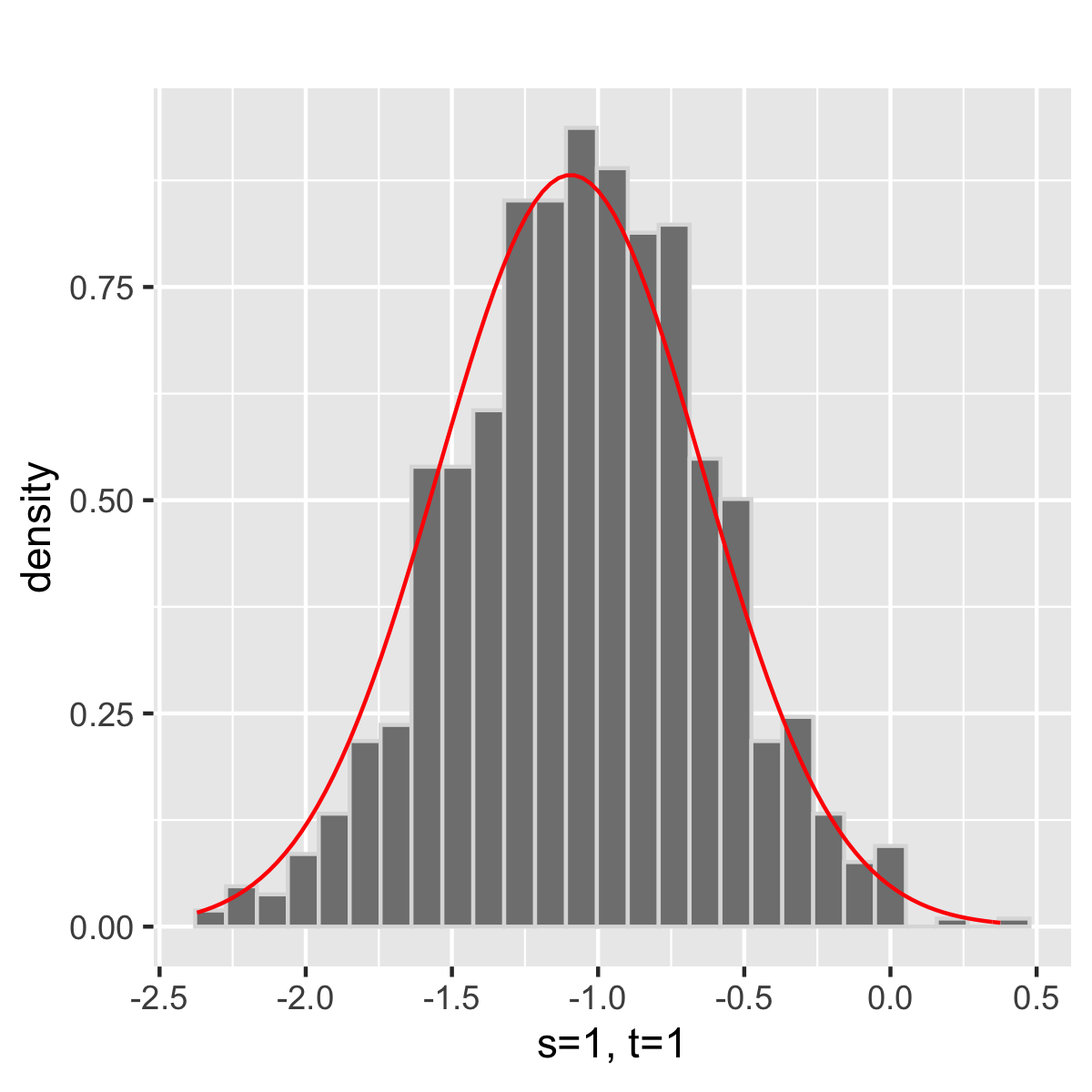
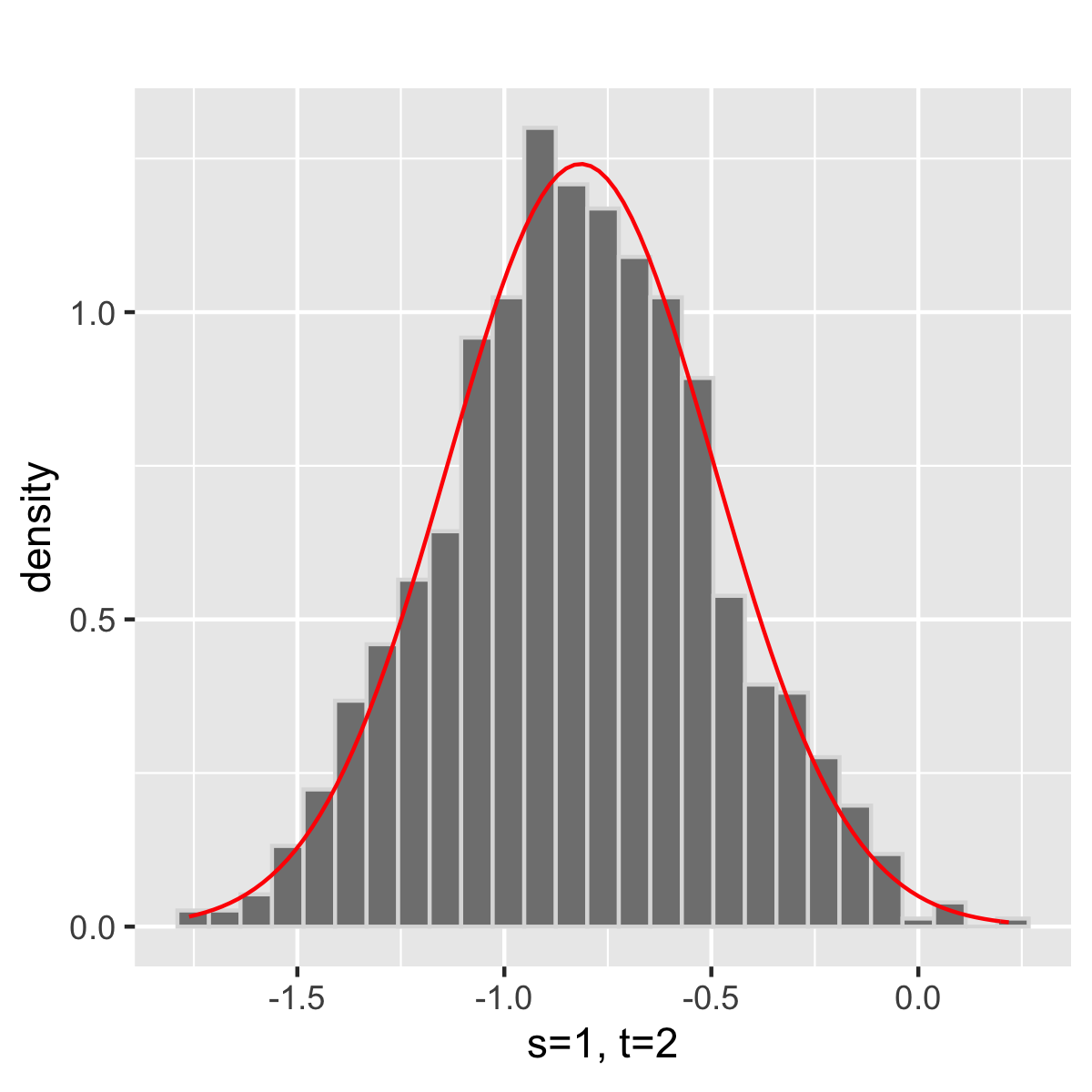
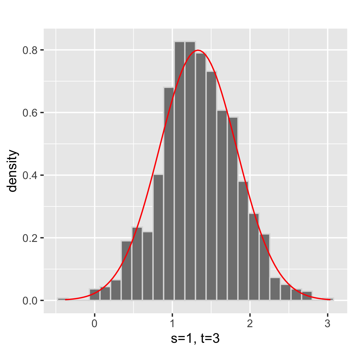
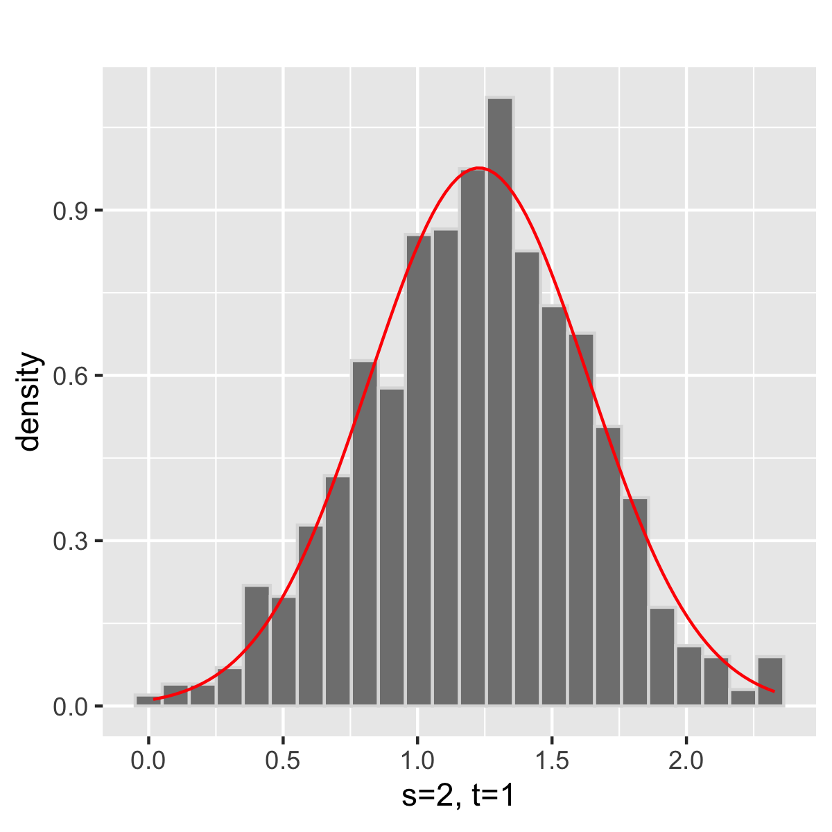
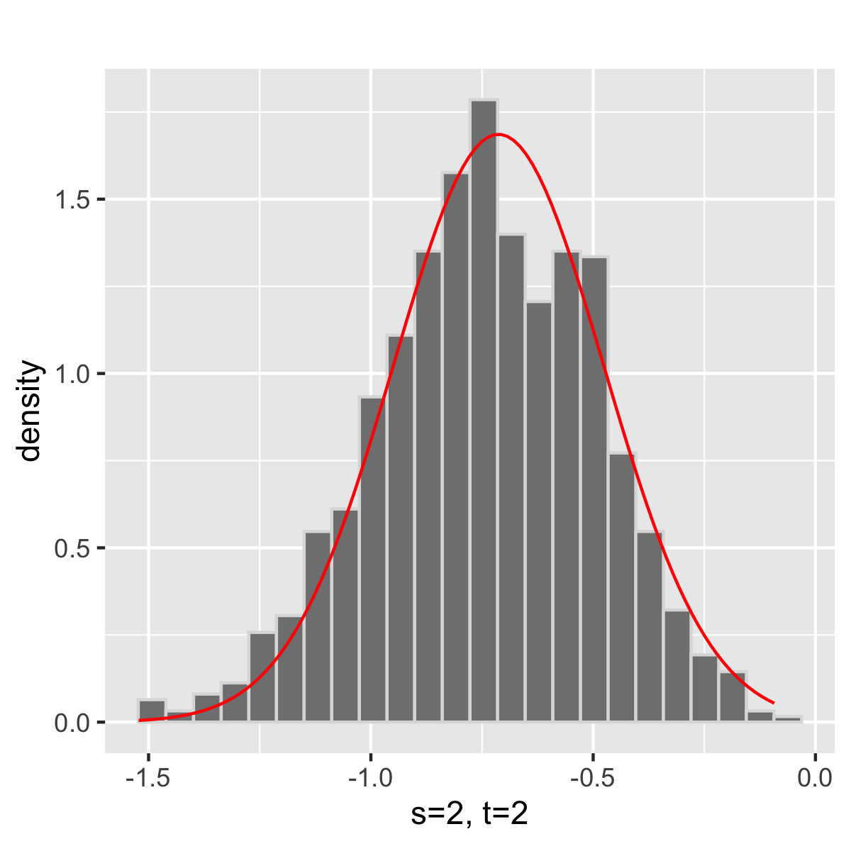
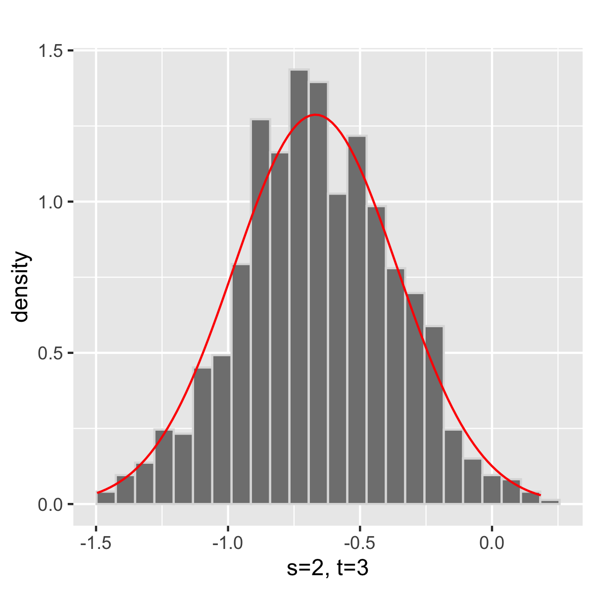
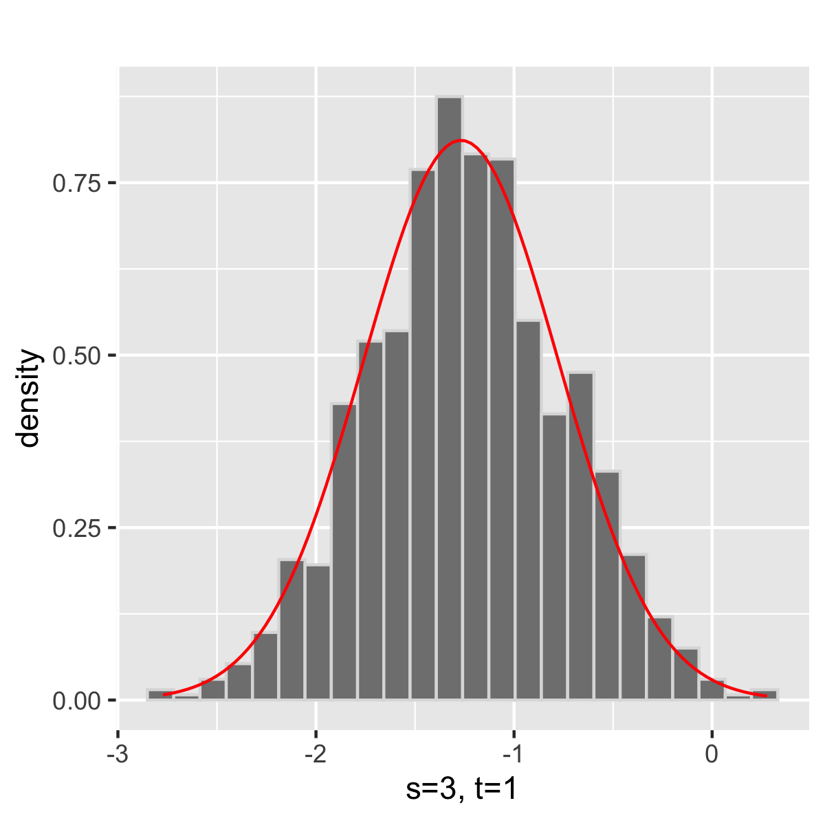
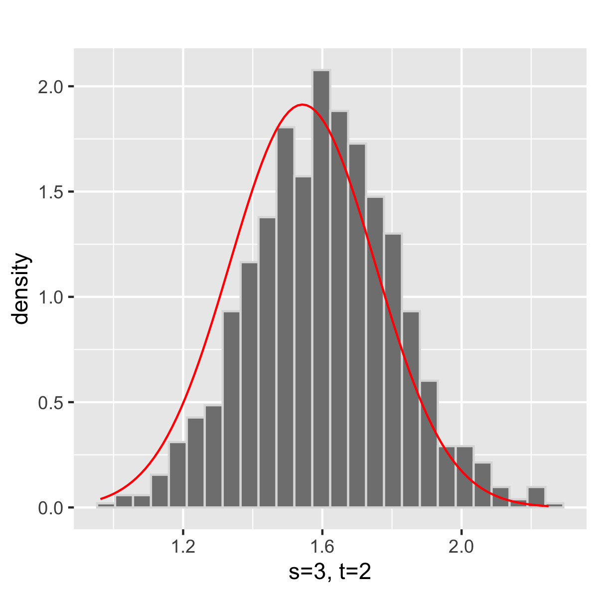
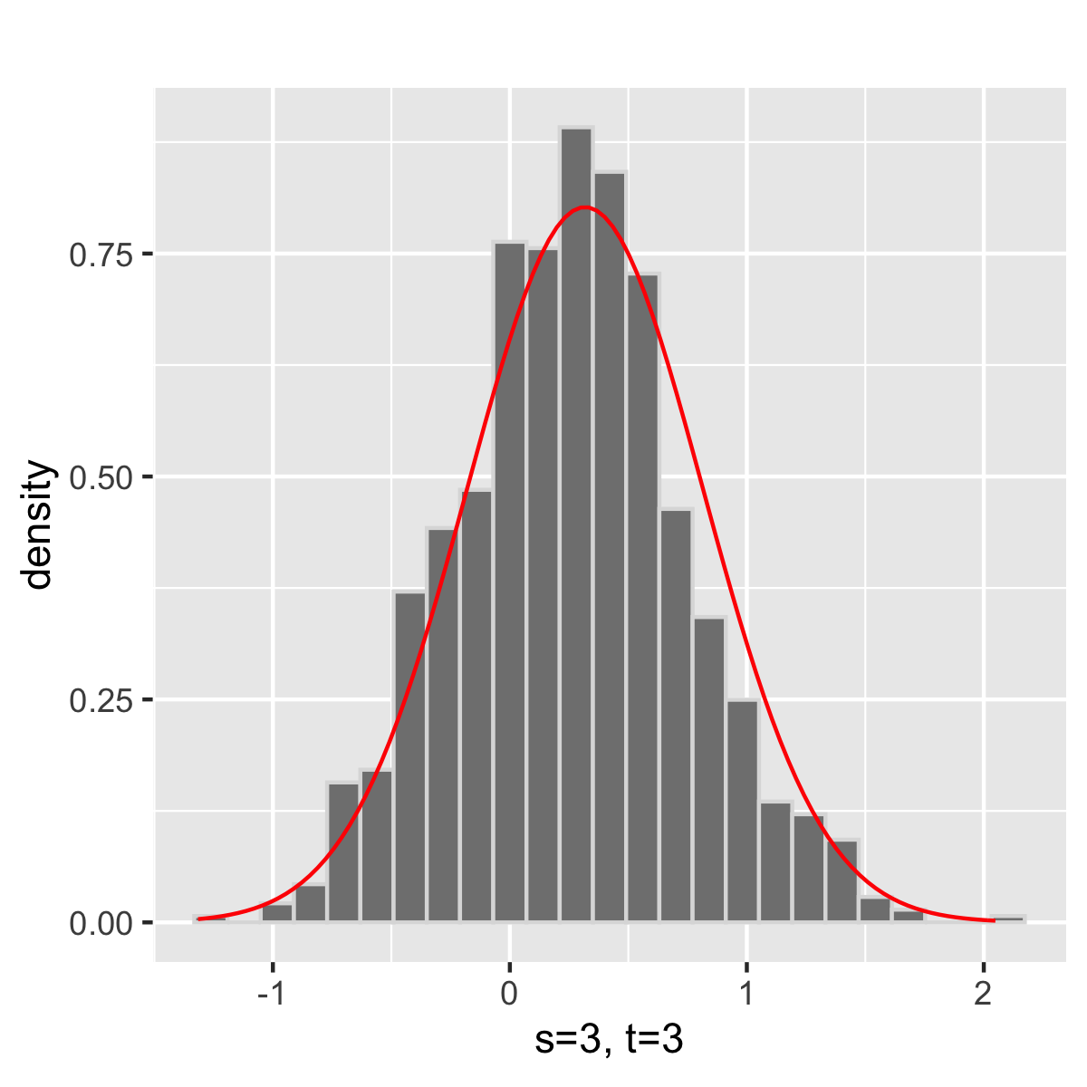
Figure 1: Plots for the empirical distributions of the entries $(\mathbf{W}_{\mathbf{U}}^{\top}\hat{\mathbf{R}}^{(1)}\mathbf{W}_{\mathbf{V}}-\mathbf{R}^{(1)})_{st}$. The histograms are based on $1000$ samples of multi-layer SBM graphs on $n=2000$ vertices with $m=3$ layers and $K=3$ blocks. The red lines are the probability density functions of the normal distributions with parameters given in Theorem 5.

We next consider the problem of determining whether or not two graphs $\mathbf{A}^{(i)}$ and $\mathbf{A}^{(j)}$ have the same distribution, i.e., we wish to test $\mathbb{H}_{0}\colon\mathbf{R}^{(i)}=\mathbf{R}^{(j)}$ against $\mathbb{H}_{A}\colon\mathbf{R}^{(i)}\not=\mathbf{R}^{(j)}$. We once again generate $1000$ Monte Carlo replicates where, for each replicate, we generate a directed multi-layer SBM with $m=3$ graphs, $K=3$ blocks using a similar setting to that described at the beginning of this section, except now we set either $\mathbf{B}^{(2)}=\mathbf{B}^{(1)}$ or $\mathbf{B}^{(2)}=\mathbf{B}^{(1)}+\frac{1}{n}\mathbf{1}\mathbf{1}^{\top}$. These two choices for $\mathbf{B}^{(2)}$ correspond to the null and local alternative, respectively. For each Monte Carlo replicate we compute the test statistic in Theorem 6 and compare its empirical distributions under the null and alternative hypothesis against the central and non-central $\chi^{2}$ distribution with $9$ degrees of freedom. The results are summarized in Figure 2 and we see that $T_{12}$ are indeed well approximated by the $\chi^{2}_{9}$ distributions.

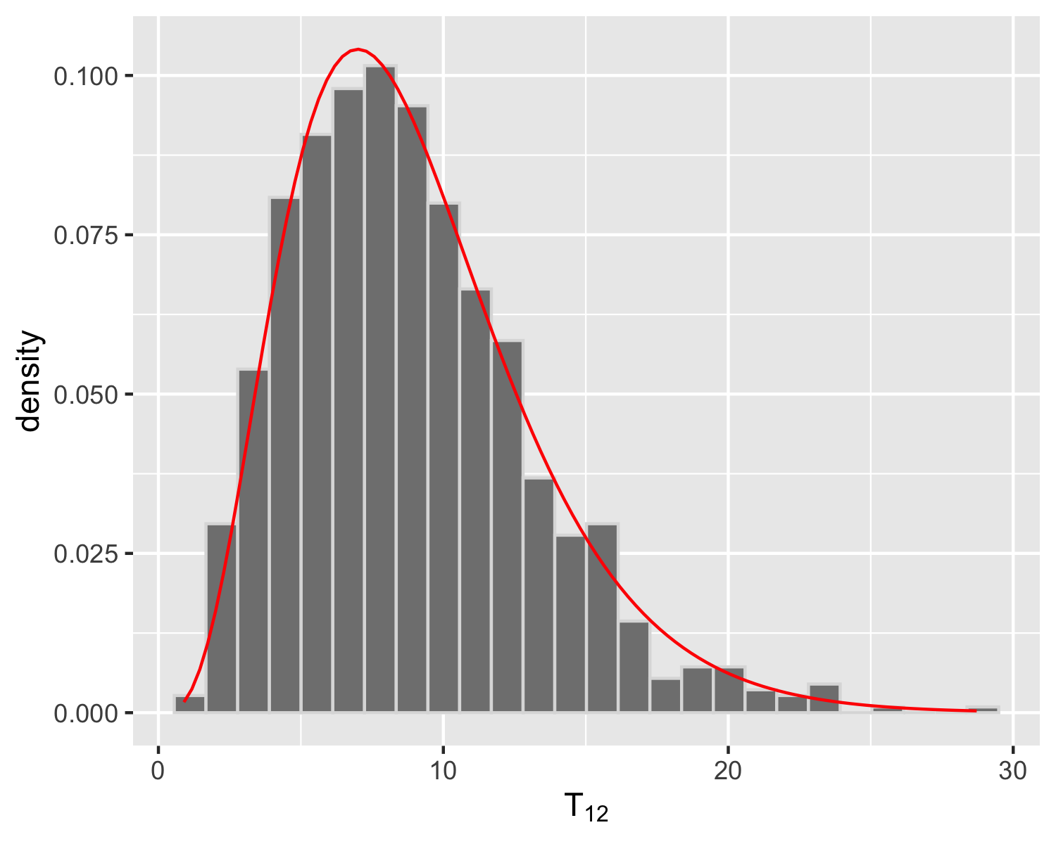
(a) null hypothesis

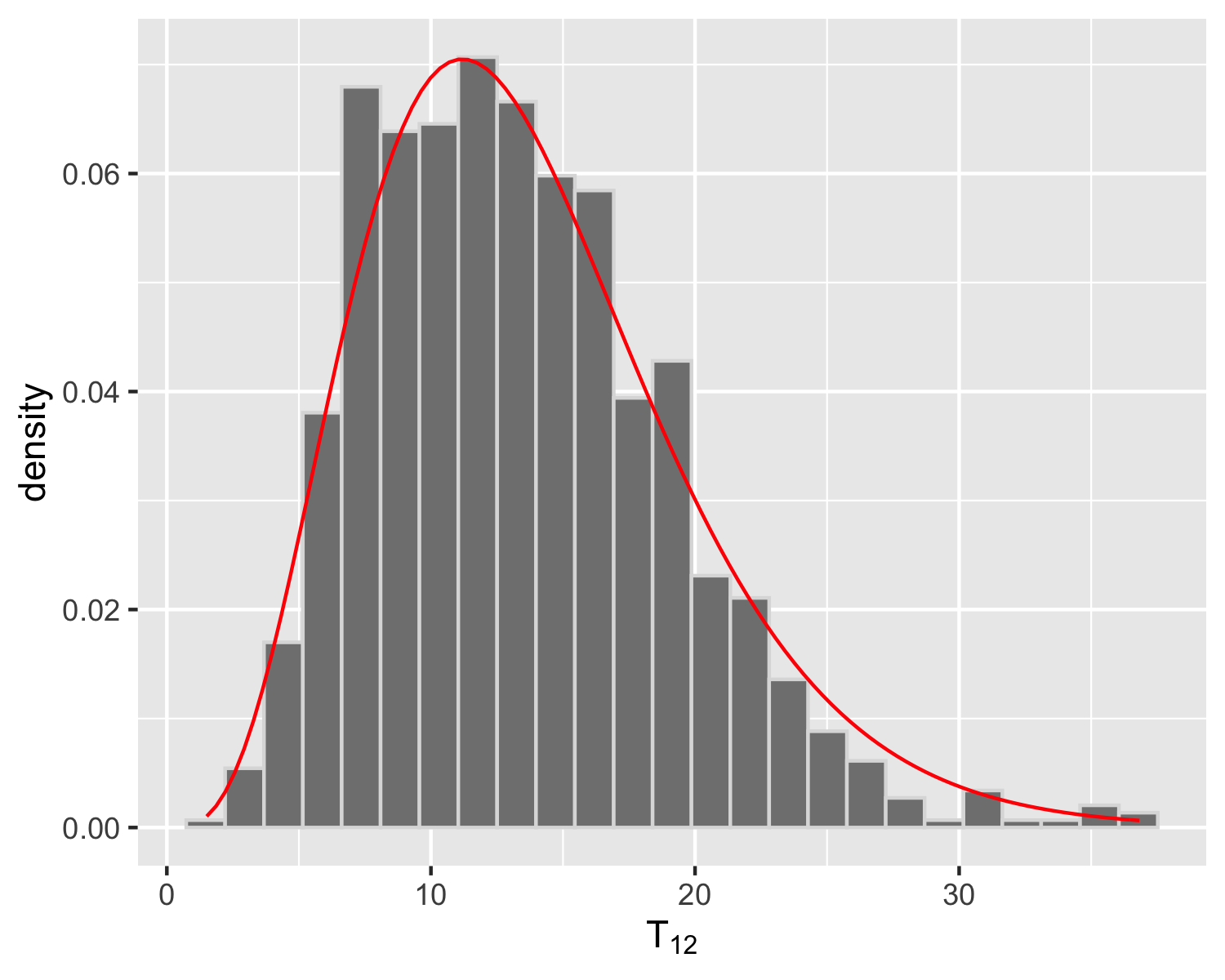
(b) alternative hypothesis

Figure 2: Plots for the empirical distributions of $T_{12}$ under either the null or local alternative hypothesis. The histograms are based on $1000$ samples of multi-layer SBM graphs on $n=2000$ vertices with $m=3$ layers and $K=3$ blocks. The red lines are the probability density functions for the central and non-central chi-square distributions with $9$ degrees of freedom and non-centrality parameters given in Theorem 6.

4.2 MultiNeSS model

In Remark 6, we introduce the generalized model where $\{\mathbf{P}^{(i)}\}$ all share some invariant subspaces but also have possibly distinct subspaces, and introduce how to estimate the subspaces with our algorithm. In this section we will show the performance of our algorithm for recovering the common and individual structures in a collection of matrices generated from the MultiNeSS model [macdonald2022latent] with Gaussian errors. More specifically, for any $i\in[m]$, let $\mathbf{P}^{(i)}$ be a $n\times n$ matrix of the form

$$\mathbf{P}^{(i)}=\mathbf{X}_{c}\mathbf{X}_{c}^{\top}+\mathbf{X}_{s}^{(i)}\mathbf{X}_{s}^{(i)\top},$$

where $\mathbf{X}_{c}\in\mathbb{R}^{n\times d_{1}},\mathbf{X}_{s}^{(i)}\in\mathbb{R}^{n\times d_{2}}$. Let $\mathbf{F}:=\mathbf{X}_{c}\mathbf{X}_{c}^{\top}$ be the common structure across all $\{\mathbf{P}^{(i)}\}$, and let $\mathbf{G}^{(i)}:=\mathbf{X}_{s}^{(i)}\mathbf{X}_{s}^{(i)\top}$ be the individual structure for $\mathbf{P}^{(i)}$. We then generate $\mathbf{A}^{(i)}=\mathbf{P}^{(i)}+\mathbf{E}^{(i)}$ where $\mathbf{E}^{(i)}$ is a symmetric random matrix whose upper triangular entries are iid $N(0,\sigma^{2})$ random variables.

Given $\{\mathbf{A}^{(i)}\}_{i=1}^{m}$ we first compute $\hat{\mathbf{U}}^{(i)}$ as the $n\times(d_{1}+d_{2})$ matrix whose columns are the $d_{1}+d_{2}$ leading eigenvectors of $\mathbf{A}^{(i)}$ for each $i\in[m]$. Next we let $\hat{\mathbf{U}}_{c}$ be the $n\times d_{1}$ matrix whose columns are the $d_{1}$ leading left singular vectors of $[\hat{\mathbf{U}}^{(1)}|\cdots|\hat{\mathbf{U}}^{(m)}]$ and $\hat{\mathbf{U}}_{s}^{(i)}$ be the $n\times d_{2}$ matrix containing the $d_{2}$ leading left singular vectors of $(\mathbf{I}-\hat{\mathbf{U}}_{c}\hat{\mathbf{U}}_{c}^{\top})\hat{\mathbf{U}}^{(i)}$ for all $i\in[m]$. Finally we compute the estimates of $\mathbf{F},\mathbf{G}^{(i)},\mathbf{P}^{(i)}$ via

$$\hat{\mathbf{F}}=\hat{\mathbf{U}}_{c}\hat{\mathbf{U}}_{c}^{\top}\bar{\mathbf{A}}\hat{\mathbf{U}}_{c}\hat{\mathbf{U}}_{c}^{\top},\quad\hat{\mathbf{G}}^{(i)}=\hat{\mathbf{U}}_{s}^{(i)}\hat{\mathbf{U}}_{s}^{(i)\top}\mathbf{A}^{(i)}\hat{\mathbf{U}}_{s}^{(i)}\hat{\mathbf{U}}_{s}^{(i)\top},\quad\hat{\mathbf{P}}^{(i)}=\hat{\mathbf{U}}_{c,s}^{(i)}\hat{\mathbf{U}}_{c,s}^{(i)\top}\mathbf{A}^{(i)}\hat{\mathbf{U}}_{c,s}^{(i)}\hat{\mathbf{U}}_{c,s}^{(i)\top},$$

where $\bar{\mathbf{A}}=m^{-1}\sum_{i=1}^{m}\mathbf{A}^{(i)}$ and $\hat{\mathbf{U}}_{c,s}^{(i)}=[\hat{\mathbf{U}}_{c}|\hat{\mathbf{U}}_{s}^{(i)}]$.

We use the same setting as that in Section 5.2 in [macdonald2022latent]. More specifically we fix $d_{1}=d_{2}=2,\sigma=1$, and either fix $m=8$ and vary $n\in\{200,300,400,500,600\}$ or fix $n=400$ and vary $m\in\{4,8,12,15,20,30\}$. The estimation error for $\hat{\mathbf{F}},\{\hat{\mathbf{G}}^{(i)}\}$ and $\{\hat{\mathbf{P}}^{(i)}\}$ are also evaluated using the same metric as that in [macdonald2022latent], i.e., we compute

$$\text{ErrF}=\frac{\|\hat{\mathbf{F}}-\mathbf{F}\|_{\tilde{F}}}{\|\mathbf{F}\|_{\tilde{F}}},\quad\text{ErrG}=\frac{1}{m}\sum_{i=1}^{m}\frac{\|\hat{\mathbf{G}}^{(i)}-\mathbf{G}^{(i)}\|_{\tilde{F}}}{\|\mathbf{G}^{(i)}\|_{\tilde{F}}},\quad\text{ErrP}=\frac{1}{m}\sum_{i=1}^{m}\frac{\|\hat{\mathbf{P}}^{(i)}-\mathbf{P}^{(i)}\|_{\tilde{F}}}{\|\mathbf{P}^{(i)}\|_{\tilde{F}}},$$

where $\|\cdot\|_{\tilde{F}}$ denote the Frobenius norm of a matrix after setting its diagonal entries to $0$. The results are summarized in Figure 3 and Figure 4. Comparing the relative Frobenius norm errors in Figure 3 and Figure 4 with those in Figure 2 of [macdonald2022latent], we see that the two set of estimators have comparable performance. Nevertheless, our algorithm is slightly better for recovering the common structure (smaller ErrF) while the algorithm in [macdonald2022latent] is slightly better for recovering individual structure (smaller ErrG). Finally for recovering the overall edge probabilities $\{\mathbf{P}^{(i)}\}$, our ErrPs are always smaller than theirs. Indeed, as $n$ varies from $200$ to $600$, the mean of our ErrP varies from about $0.076$ to $0.044$ while the mean in [macdonald2022latent] varies from about $0.08$ to $0.05$. Simialrly, as $m$ varies from $4$ to $30$, the mean of our ErrP varies from about $0.056$ to $0.051$ while the mean in [macdonald2022latent] varies from about $0.07$ to $0.06$. In summary, while the two algorithms yield estimates with comparable performance, our algorithm has some computational advantage as (1) it is not an interative procedure and (2) it does not require any tuning parameters (note that the embedding dimensions $d_{1}$ and $d_{2}$ are generally not tuning parameters but rather chosen via some dimension selection procedure).

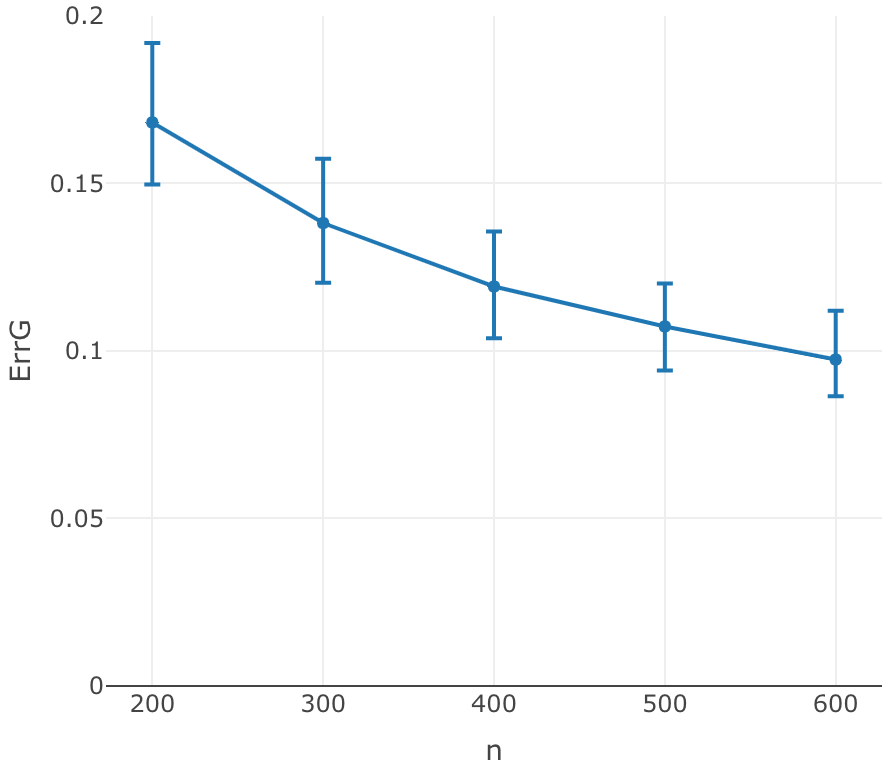
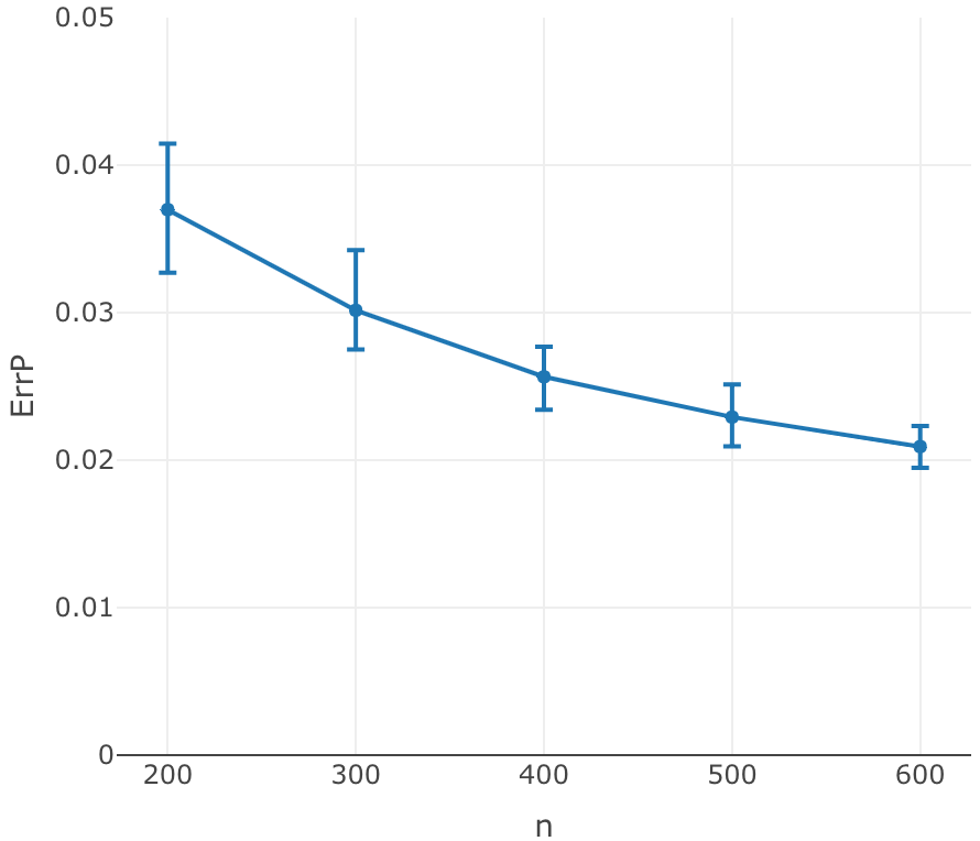
Figure 3: Relative Frobenius norm errors for the common structure (left panel), the individual structure (middle panel), and the overall expectation of the matrix (right panel) with $d_{1}=d_{2}=2,\sigma=1,m=8$ and $n\in\{200,300,400,500,600\}$. The figures display the mean, $0.05$ and $0.95$ quantile points, over $100$ independent Monte Carlo replications.

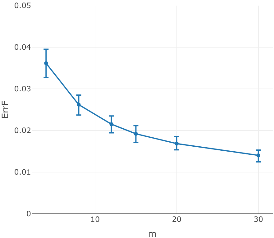
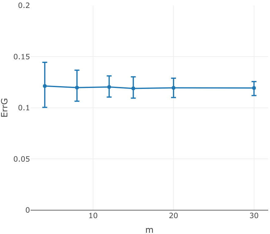
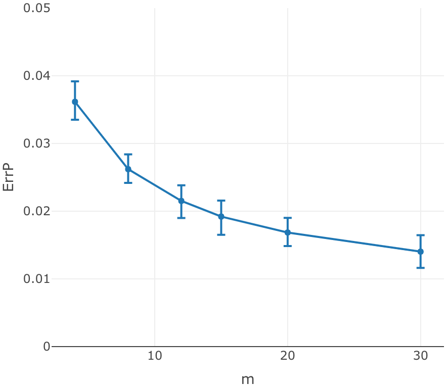
Figure 4: Relative Frobenius norm errors for the common structure (left panel), the individual structure (middle panel), and the overall expectation of the matrix (right panel) with $d_{1}=d_{2}=2,\sigma=1,n=400$ and $m\in\{4,8,12,15,20,30\}$. The figures display the mean, $0.05$ and $0.95$ quantile points, over $100$ independent Monte Carlo replications.

4.3 Distributed PCA

We now demonstrate our theoretical results for distributed PCA by simulations. Let $m$, $n$ and $D$ be positive integers and $\{X_{j}^{(i)}\}_{i\in[m],j\in[n]}$ be a collection of $mn$ iid random vectors in $\mathbb{R}^{D}$ with $X_{j}^{(i)}\sim\mathcal{N}(\mathbf{0},\bm{\Sigma})$. Here $\bm{\Sigma}=\mathbf{U}\bm{\Lambda}\mathbf{U}^{\top}+(\mathbf{I}-\mathbf{U}\mathbf{U}^{\top})$ with $\bm{\Lambda}=\operatorname{diag}(\lambda,\lambda/2,\lambda/4)$. The matrix $\mathbf{U}$ is sampled uniformly from the set of $D\times 3$ matrices $\mathbf{O}$ with $\mathbf{O}^{\top}\mathbf{O}=\mathbf{I}$ and thus $\bm{\Sigma}$ has $d=3$ spiked eigenvalues. Given $\{X_{j}^{(i)}\}_{i\in[m],j\in[n]}$ we partition the data into $m$ subsamples, each having $n$ vectors, and then estimate $\mathbf{U}$ using Algorithm 1 with $d_{i}\equiv d=3$.

We obtain an empirical distribution for $\mathbf{W}^{\top}\hat{u}_{1}-u_{1}$ based on $1000$ Monte Carlo replications with $m=50,n=2000,D=1600$ and $\lambda=80$ and compare it against the limiting Gaussian distribution specified in Theorem 8. Here $\hat{u}_{1}$ and $u_{1}$ denote the first row of $\hat{\mathbf{U}}$ and $\mathbf{U}$, respectively. The Henze-Zirkler’s normality test fails to reject (at significance level $0.05$) the null hypothesis that the empirical distribution follows a multivariate normal distribution. For more details see Figure 5 for histograms plots of the marginal distributions of $\big{(}\mathbf{W}^{\top}\hat{u}_{1}-u_{1})$ and Figure 6 for scatter plots of $\big{(}\mathbf{W}^{\top}\hat{u}_{1}-u_{1}\bigr{)}_{i}$ vs $\bigl{(}\mathbf{W}^{\top}\hat{u}_{1}-u_{1}\bigr{)}_{j}$.

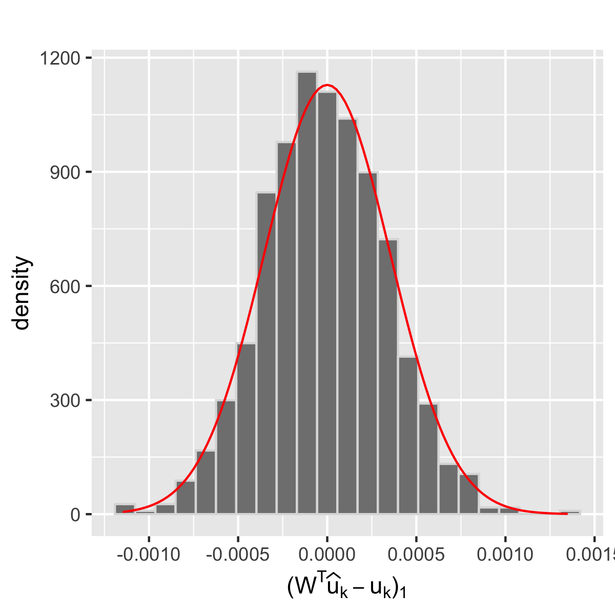
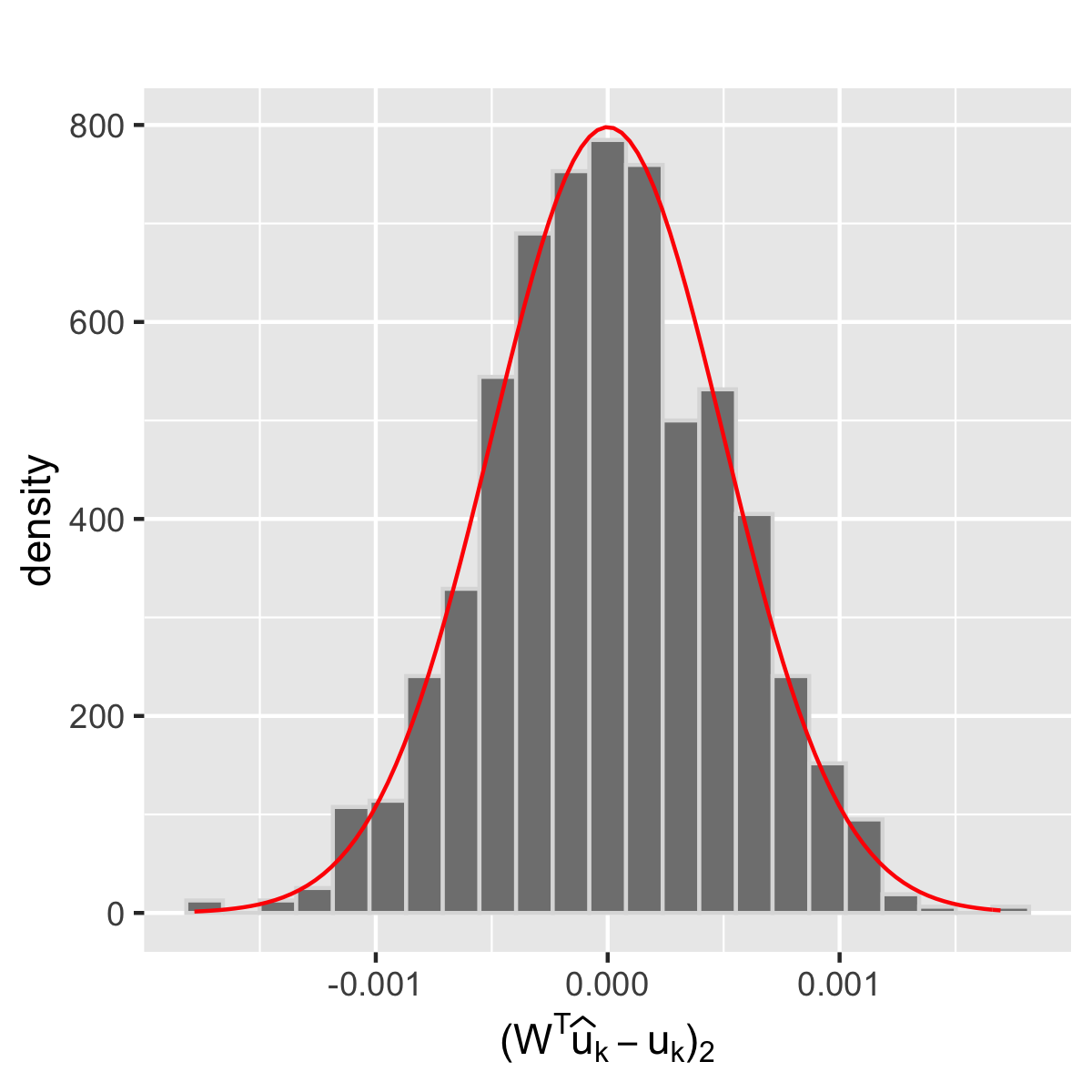
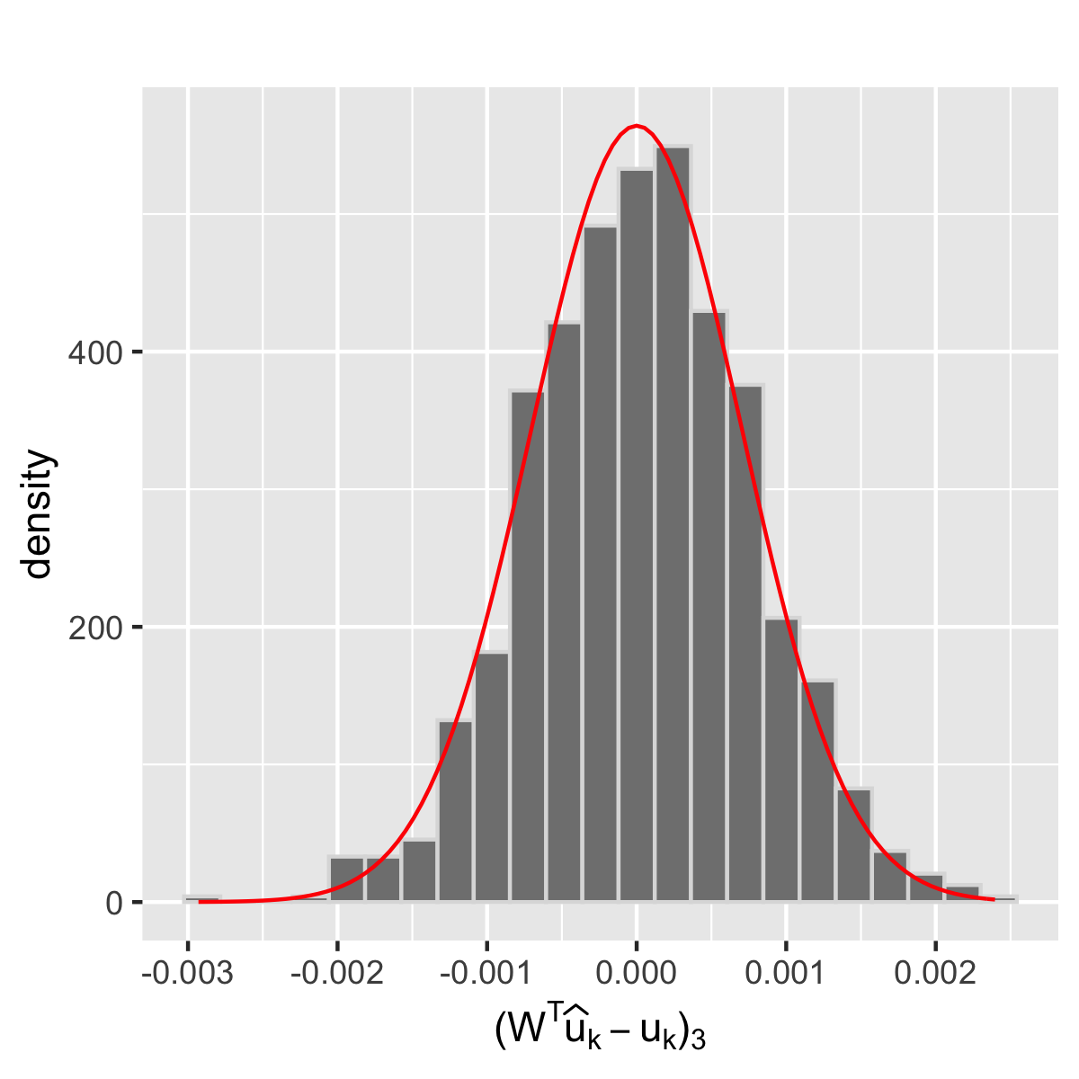
Figure 5: Empirical histograms for the marginal distributions of the entries of $\mathbf{W}^{\top}\hat{u}_{1}-u_{1}$ based on independent $1000$ Monte Carlo replicates with $m=50,n=2000,D=1600,\lambda=80$. The red lines are the pdf for the Gaussian distributions with parameters specified as in Theorem 8.

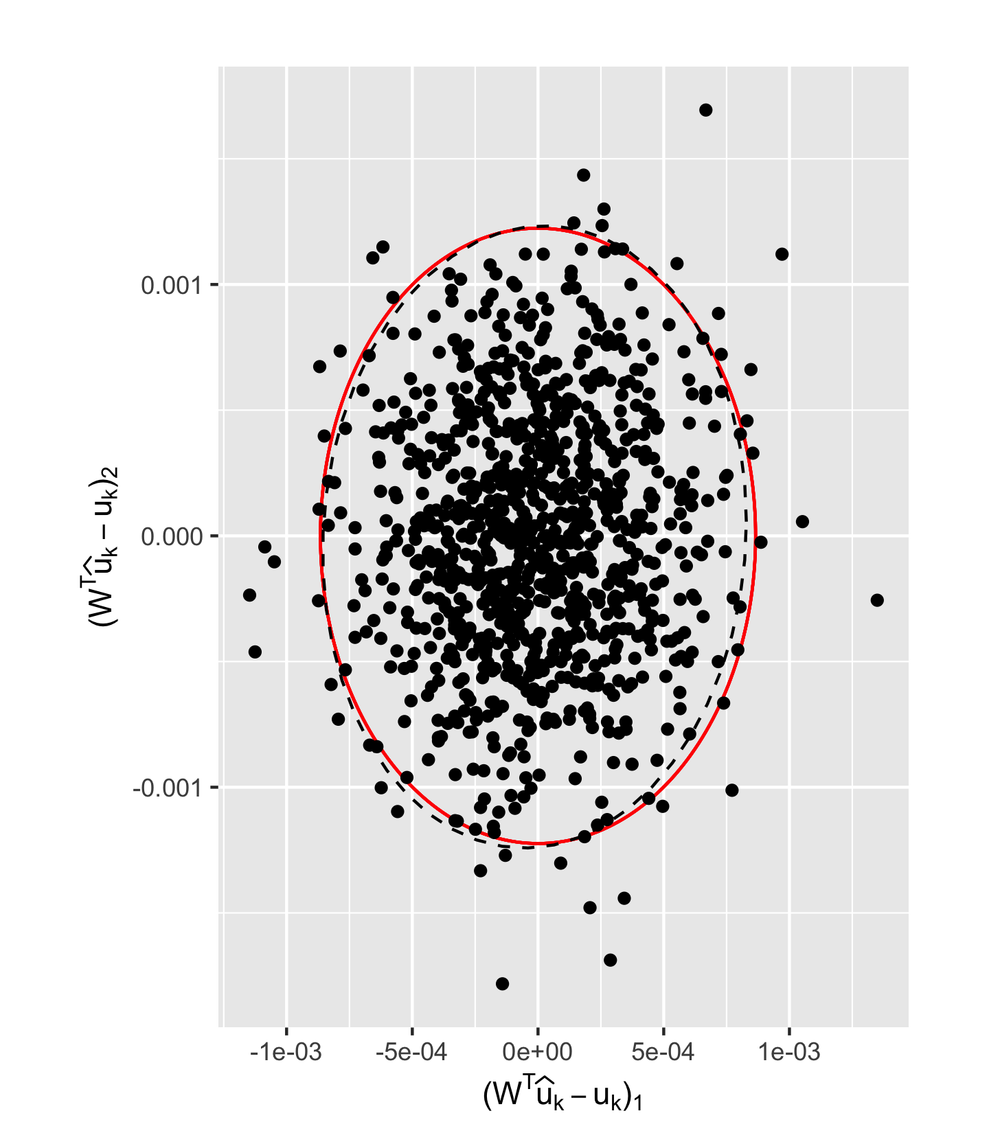
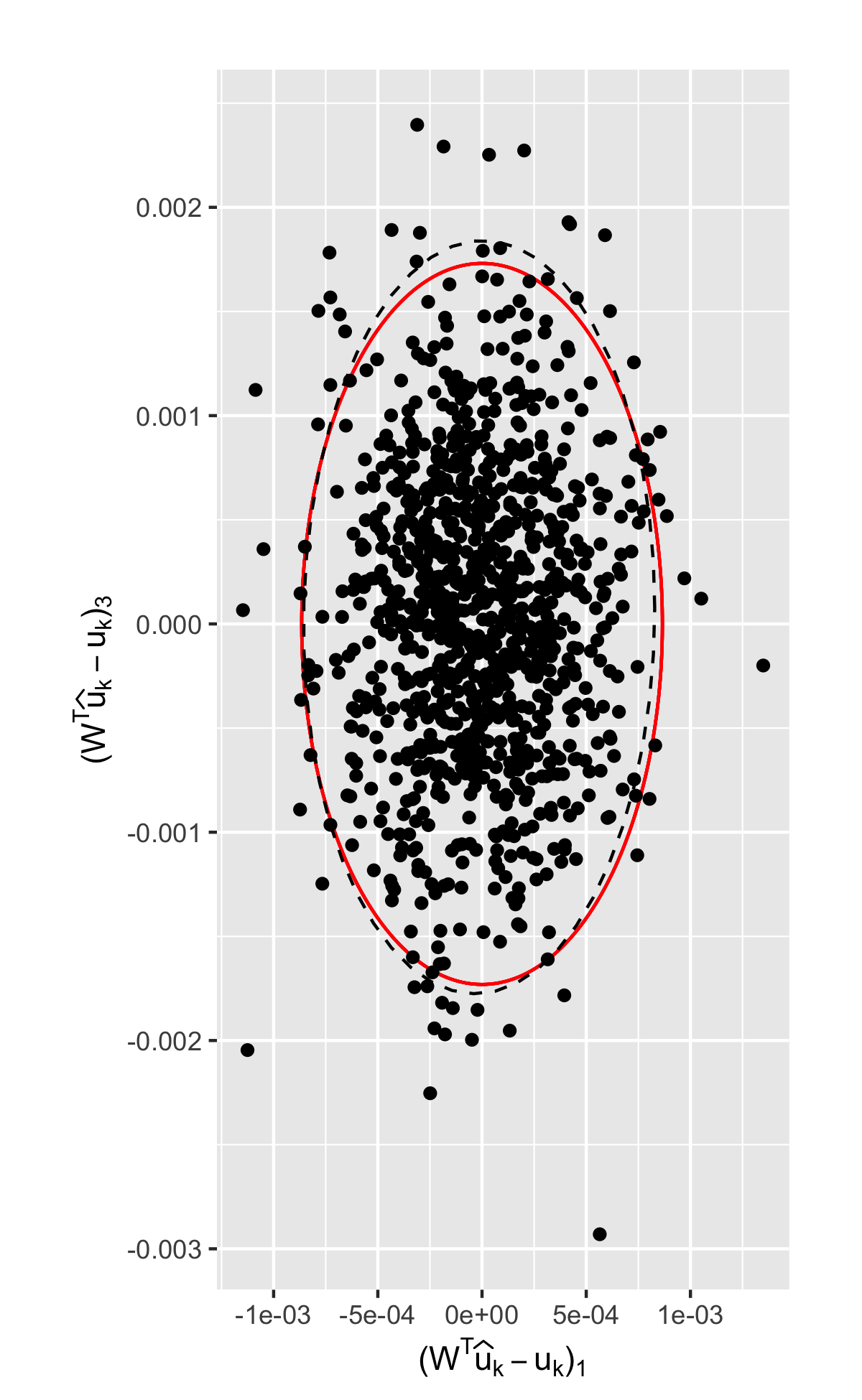
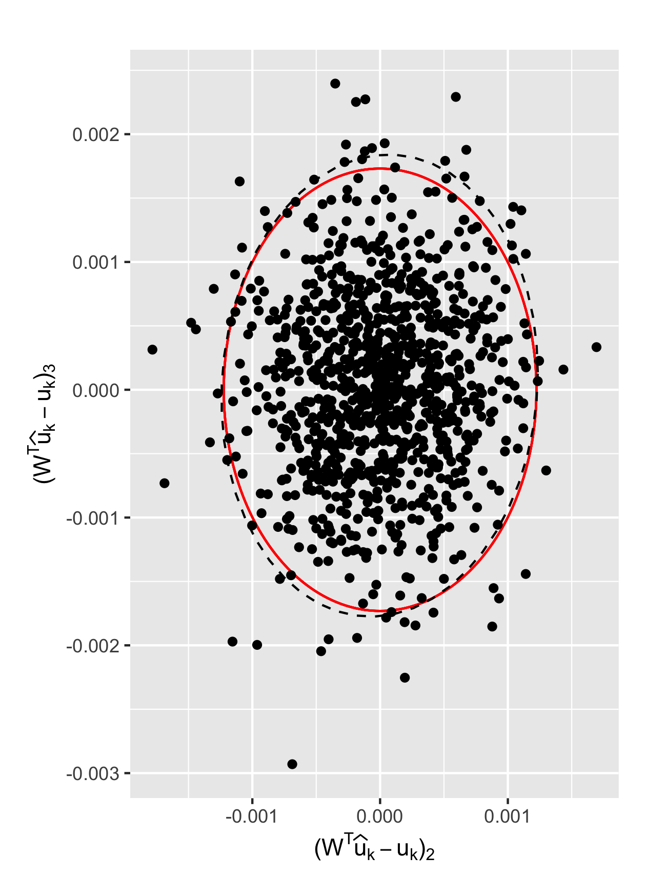
Figure 6: Bivariate plots for the empirical distribution between the entries of $\mathbf{W}^{\top}\hat{u}_{1}-u_{1}$ based on $1000$ Monte Carlo replicates with $m=50,n=2000,D=1600,\lambda=80$. Dashed black ellipses represent $95\%$ level curves for the empirical distributions while solid red ellipses represent $95\%$ level curves for the theoretical distributions as specified in Theorem 8.

4.4 Connectivity of brain networks

In this section we use the test statistic $T_{ij}$ in Section 2.3 to measure similarities between different connectomes constructed from the HNU1 study [zuo2014open]. The data consists of diffusion magnetic resonance imaging (dMRI) records for $30$ healthy adults subjects where each subject received $10$ dMRI scans over the span of one month. The resulting $m=300$ dMRIs are then converted into undirected and unweighted graphs on $n=200$ vertices by registering the brain regions for these images to the CC200 atlas of [craddock2012whole].

Taking the $m=300$ graphs as one realization from an undirected COSIE model, we first apply Algorithm 1 to extract the “parameters estimates” $\hat{\mathbf{U}},\hat{\mathbf{V}},\{\hat{\mathbf{R}}^{(i)}\}_{i=1}^{300}$ associated with these graph. The initial embedding dimensions $\{d_{i}\}_{i=1}^{300}$, which range from $5$ to $18$, and the final embedding dimension $d=11$ are all selected using the (automatic) dimensionality selection procedure described in [zhu2006automatic]. Given the quantities $\hat{\mathbf{U}},\hat{\mathbf{V}}$ and $\{\hat{\mathbf{R}}^{(i)}\}$ we compute $\hat{\mathbf{P}}^{(i)}=\hat{\mathbf{U}}\hat{\mathbf{R}}^{(i)}\hat{\mathbf{U}}^{\top}$ for each graph $i$ (and truncate the entries of the resulting $\hat{\mathbf{P}}^{(i)}$ to lie in $[0,1]$) before computing $\{\hat{\bm{\Sigma}}^{(i)}\}_{i=1}^{300}$ using the formula in Remark 9. Finally we compute the test statistic $T_{ij}$ for all pairs $i,j\in[m]$, $i\not=j$ as defined in Theorem 6.

The left panel of Figure 7 shows the matrix of $T_{ij}$ values for all pairs $(i,j)\in[m]\times[m]$ with $i\not=j$ while the right panel presents the $p$-values associated with these $T_{ij}$ (as compared against the $\chi^{2}$ distribution with $\tbinom{d}{2}=66$ degrees of freedom). Note that, for ease of presentation we have rearranged the $m=300$ graphs so that graphs for the same subject are grouped together and furthermore we only include, on the $x$ and $y$ axes marks, the labels for the subjects but not the individual scans within each subject. We see that our test statistic $T_{ij}$ can discern between scans from the same subject (where $T_{ij}$ are generally small) and scans from different subjects (where $T_{ij}$ are quite large). Indeed, given any two scans $i$ and $j$ from different subjects, the $p$-values for $T_{ij}$ (under the null hypothesis that $\mathbf{R}^{(i)}=\mathbf{R}^{(j)}$) is always smaller than $0.01$. Figure 8 shows the ROC curve when we use $T_{ij}$ to classify whether a pair of graphs represents scans from the same subject (specificity) or from different subjects (sensitivity). The corresponding AUC is $0.970$ and is thus close to optimal.

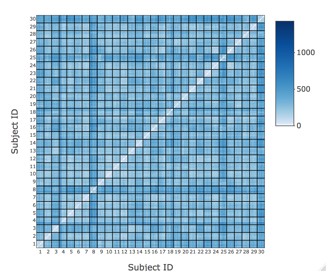
(a) $T_{ij}$

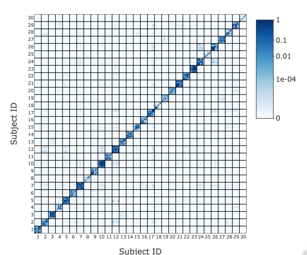
(b) $p$-values

Figure 7: Left panel: test statistic $T_{ij}$ for each pair of brain connectivity networks. Right panel: $p$-values associated with the $T_{ij}$ when compared against the chi-square distribution with $66$ degrees of freedom.

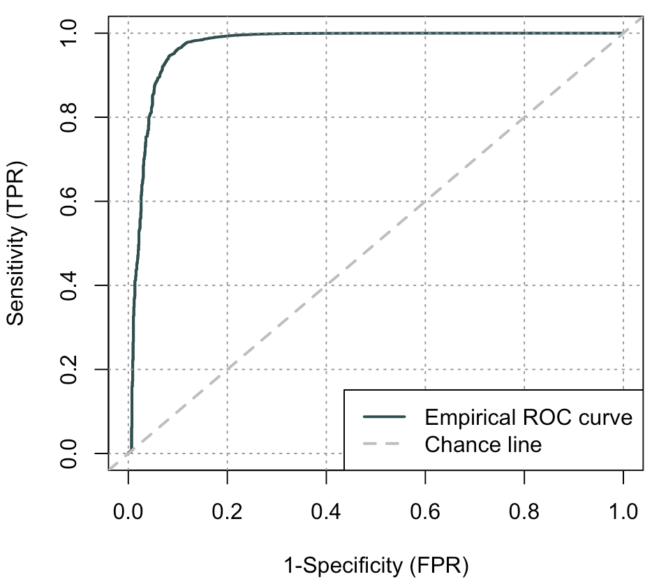
Figure 8: ROC curve for classifiying if a pair of graphs represent scans from the same subject (specificity) or from different subjects (sensitivity) as determined by thresholding the values of $T_{ij}$. The corresponding AUC is $0.970$.

The HNU1 data have also been analyzed in [arroyo2019inference]. In particular, [arroyo2019inference] proposes $\|\hat{\mathbf{R}}^{(i)}-\hat{\mathbf{R}}^{(j)}\|_{F}^{2}$ as test statistic, and instead of computing $p$-values from some limiting distribution directly, [arroyo2019inference] calculates empirical $p$-values by using 1) a parametric bootstrap approach; 2) the asymptotic null distribution of $\|\hat{\mathbf{R}}^{(i)}-\hat{\mathbf{R}}^{(j)}\|_{F}^{2}$. By neglecting the effect of the bias term $\mathbf{H}^{(i)}$, [arroyo2019inference] approximates the null distribution of $\|\hat{\mathbf{R}}^{(i)}-\hat{\mathbf{R}}^{(j)}\|_{F}^{2}$ as a generalized $\chi^{2}$ distribution, and estimates it by Monte Carlo simulations of a mixture of normal distributions with the estimate $\hat{\bm{\Sigma}}^{(i)}$ and $\hat{\bm{\Sigma}}^{(j)}$. Comparing the $p$-values of our testing in Figure 7 with the results obtained by their two methods in Figure 15, we see that for different methods the ratios of the $p$-values for the pairs from the same subject and that for the pairs from different subject are very similar. Thus both test statistics can detect whether the pairs of graphs are from the same subject well. Our test statistic however has the benefit that its $p$-value is computed using large-sample $\chi^{2}$ approximation and is thus much less computationally intensive compared to test procedures which use bootstrapping and other Monte Carlo simulations.

4.5 Worldwide food trading networks

For the second example we use the trade networks between countries for different food and agriculture products during the year $2018$. The data is collected by the Food and Agriculture Organization of the United Nations and is available at https://www.fao.org/faostat/en/#data/TM. We construct a collection of networks, one for each product, where vertices represent countries and the edges in each network represent trading relationships between the countries; the resulting adjacency matrices $\{\mathbf{A}^{(i)}\}$ are directed but unweighted as we (1) set $\mathbf{A}^{(i)}_{rs}=1$ if country $r$ exports product $i$ to country $s$ and (2) ignore any links between countries $r$ and $s$ in $\mathbf{A}^{(i)}$ if their total trade amount for the $i$th product is less than two hundred thousands US dollars. Finally, we extract the intersection of the largest connected components of $\{\mathbf{A}^{(i)}\}$ and obtain $56$ networks on a set of $75$ shared vertices.

Taking the $m=56$ networks as one realization from a directed COSIE model, we apply Algorithm 1 to compute the “parameters estimates” $\hat{\mathbf{U}},\hat{\mathbf{V}},\{\hat{\mathbf{R}}^{(i)}\}_{i=1}^{56}$ associated with these graphs with initial embedding dimensions $\{d_{i}\}_{i=1}^{56}$ as well as the final embedding dimension $d$ all chosen to be $2$. Figure 9 and Figure 10 present scatter plots for the rows of $\hat{\mathbf{U}}$ and $\hat{\mathbf{V}}$, respectively; we interpret the $r$th row of $\hat{\mathbf{U}}$ (resp. $\hat{\mathbf{V}}$) as representing the estimated latent position for this country as an exporter (resp. importer). We see that there is a high degree of correlation between these “estimated” latent positions and the true underlying geographic proximities, e.g., countries in the same continent are generally placed close together in Figure 9 and Figure 10.

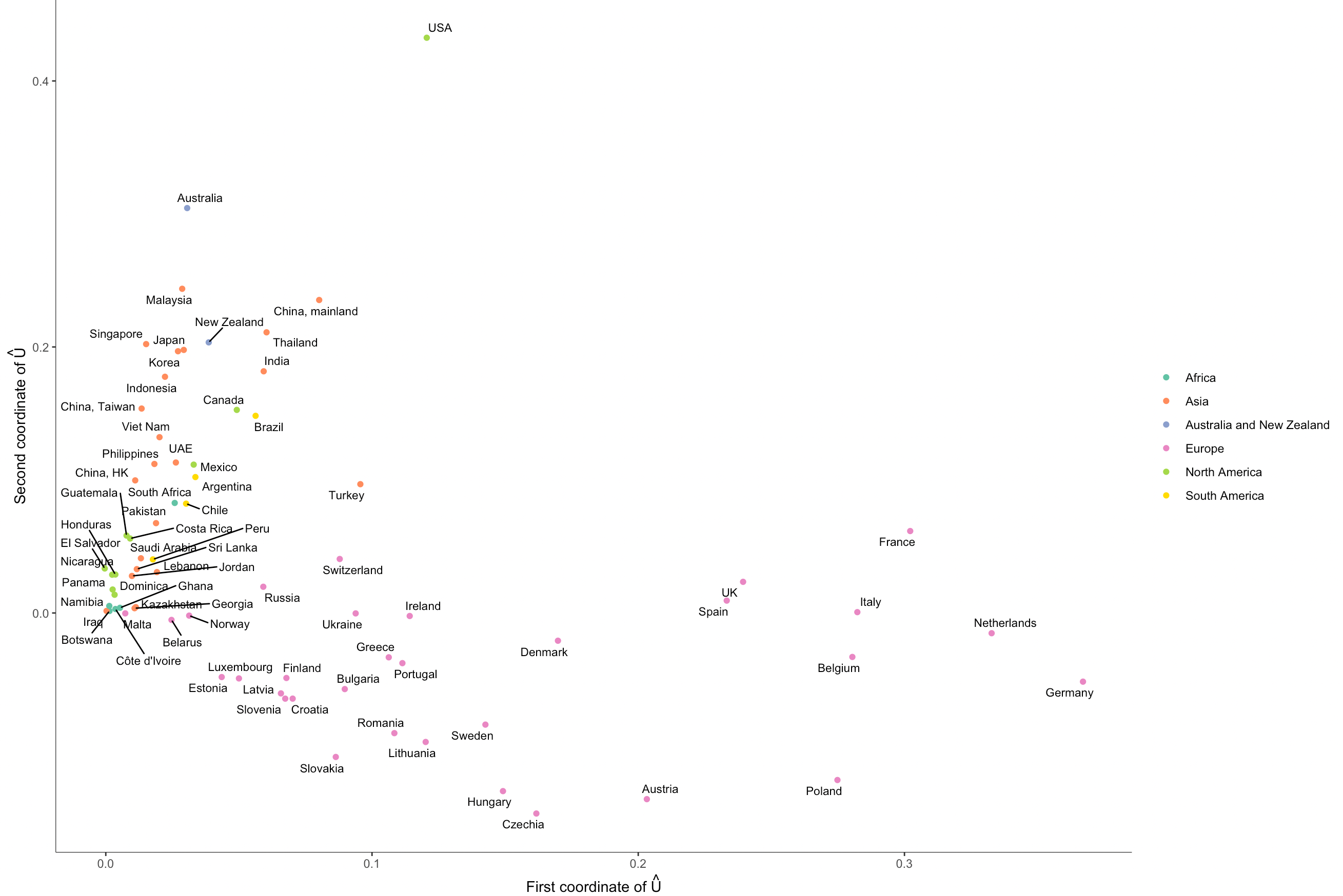
Figure 9: Latent positions of countries as exporter

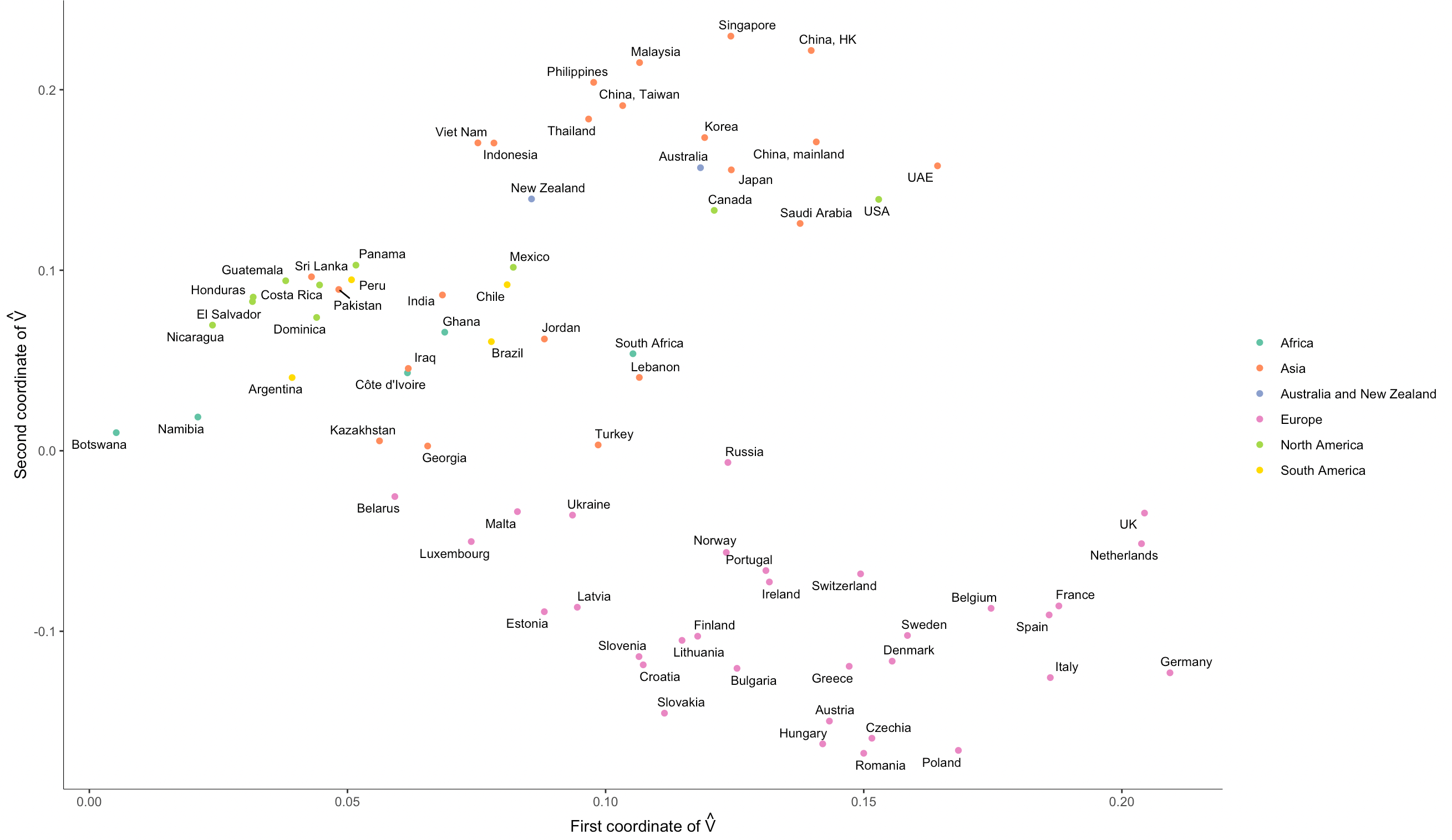
Figure 10: Latent positions of countries as importer

Next we compute the statistic $T_{ij}$ in Theorem 6 to measure the differences between $\hat{\mathbf{R}}^{(i)}$ and $\hat{\mathbf{R}}^{(j)}$ between all pairs of products $\{i,j\}$. Viewing $(T_{ij})$ as a distance matrix, we organize the food products using hierarchical clustering [johnson1967hierarchical]; see the dendogram in Figure 11. There appears to be two main clusters formed by raw/unprocessed products (bottom cluster) and processed products (top cluster), and suggest discernable differences in the trading patterns for these types of products.

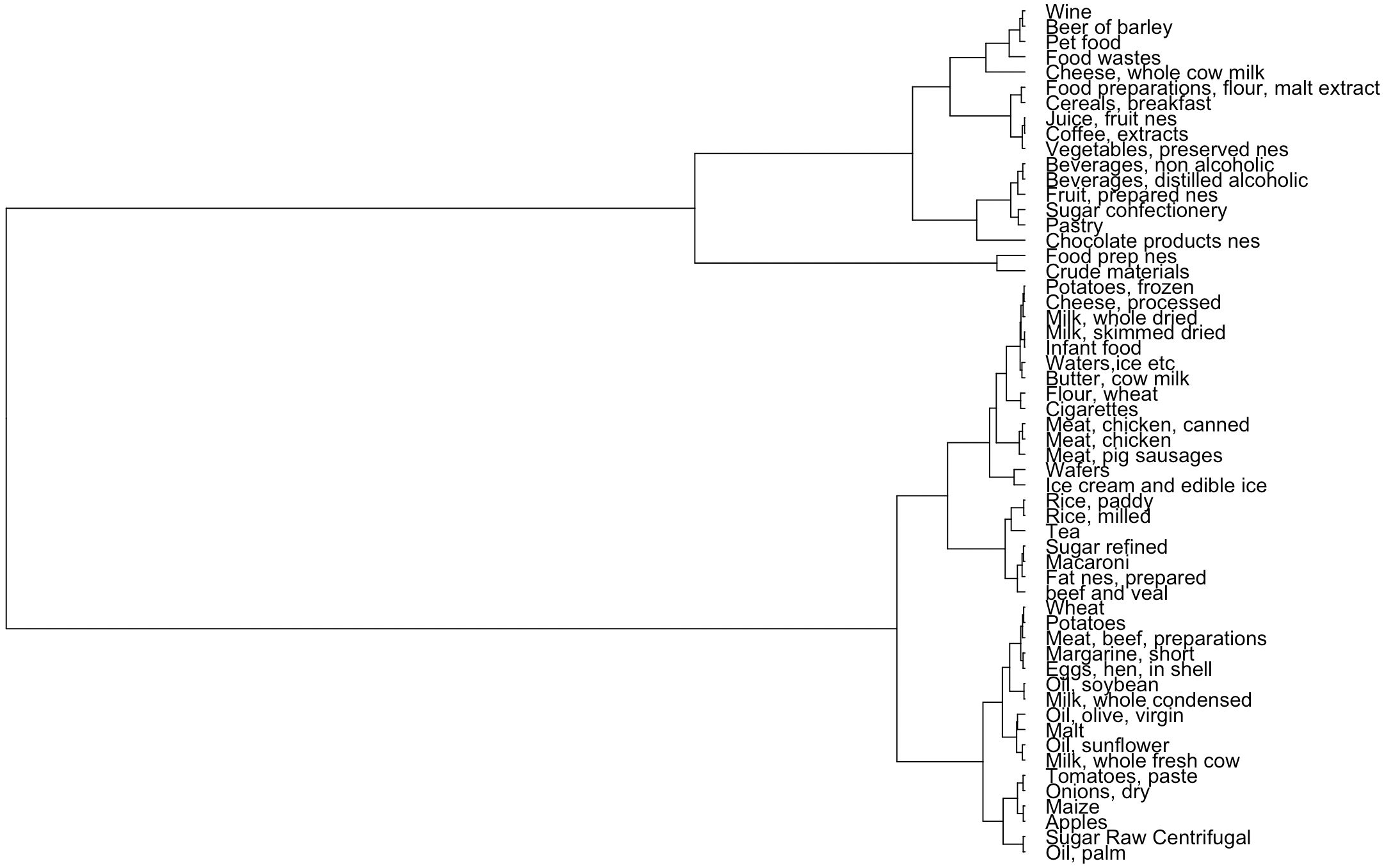
Figure 11: Hierarchical clustering of food products

The trading dataset (but for 2010) have also been analyzed in [jing2021community]. In particular, [jing2021community] studies the mixture multi-layer SBM and proposes a tensor-based algorithm to reveal memberships of vertices and memberships of layers. For the food trading networks, [jing2021community] first groups the layers, i.e., the food products, into two clusters, and then obtains the embeddings and the clustering result of the countries for each food clusters. Our results are similar to theirs. In particular their clustering of the food products also shows a difference in the trading patterns for unprocessed and processed foods while their clustering of the countries is also related to the geographical location. However, as we also compute the test statistic $T_{ij}$ for each pairs of products, we obtaine a more detailed analysis of the product relationships. In addition, as we keep the orientation for the edges (and thus our graphs are directed) we can also analyze the countries in term of both their export and import behavior, and Figures 9 and 10 show that there is indeed some difference between these behaviors, e.g., the USA and Australia are outliers as exporters but are clustered with other countries as importers.

4.6 Distributed PCA and MNIST

We now perform dimension reduction on the MNIST dataset using distributed PCA with $m\geq 2$ and compare the result against traditional PCA on the full dataset. The MNIST data consists of $60000$ grayscale images of handwritten digits of the numbers $0$ through $9$. Each image is of size $28\times 28$ pixels and can be viewed as a vector in $\mathbb{R}^{784}$ with entries in $[0,255]$. Letting $\mathbf{X}$ be the $60000\times 784$ matrix whose rows represent the images, we first extract the matrix $\hat{\mathbf{U}}$ whose columns are the $d=9$ leading principal components of $\mathbf{X}$. The choice $d=9$ is arbitrary and is chosen purely for illustrative purpose. Next we approximate $\hat{\mathbf{U}}$ using distributed PCA by randomly splitting $\mathbf{X}$ into $m\in\{2,5,10,20,50\}$ subsamples. Letting $\hat{\mathbf{U}}^{(m)}$ be the resulting approximation we compute $\min_{\mathbf{W}\in\mathcal{O}_{d}}\|\hat{\mathbf{U}}^{(m)}\mathbf{W}-\hat{\mathbf{U}}\|_{F}$. We repeat these steps for $100$ independent Monte Carlo replicates and summarize the result in Figure 12 which shows that the errors between $\hat{\mathbf{U}}^{(m)}$ and $\hat{\mathbf{U}}$ are always substantially smaller than $\|\hat{\mathbf{U}}\|_{F}=\|\mathbf{U}\|_{F}=3$. We emphasize that while the errors in Figure 12 do increase with $m$, this is mainly an artifact of the experiment setup as there is no underlying ground truth and we are only using $\hat{\mathbf{U}}$ as a surrogate for some unknown (or possibly non-existent) $\mathbf{U}$. In other words, $\hat{\mathbf{U}}$ is noise-free in this setting while $\hat{\mathbf{U}}^{(m)}$ is inherently noisy and thus it is reasonable for the noise level in $\hat{\mathbf{U}}^{(m)}$ to increases with $m$. Finally we note that, for this experiment, we have assumed that the rows of $\mathbf{X}$ are iid samples from a mixture of $10$ multivariate Gaussians with each component corresponding to a number in $\{0,1,\dots,9\}$. As a mixture of multivariate Gaussians is sub-Gaussian, the results in Section 3 remain relevant in this setting; see Remark 14.

Figure 12: Empirical estimates for the difference between the $d=9$ leading principal components of the MNIST data as computed by tradiational PCA and by distributed PCA with $m\in\{2,5,10,20,50\}$. The difference is quantified by the Procrustes error $\min_{\mathbf{W}\in\mathcal{O}_{d}}\|\hat{\mathbf{U}}^{(m)}\mathbf{W}-\hat{\mathbf{U}}\|_{F}$. The estimates (together with the $95\%$ confidence intervals) are based on $100$ independent Monte Carlo replicates.

5 Conclusion

In this paper we present a general framework for deriving limit results for distributed estimation of the leading singular vectors for a collection of matrices with shared invariant subspaces, and we apply this framework to multiple networks inference and distributed PCA. In particular, for heterogeneous random graphs from the COSIE model, we show that each row of the estimate $\hat{\mathbf{U}}$ (resp. $\hat{\mathbf{V}}$) of the left (resp. right) singular vectors converges to a multivariate normal distribution centered around the row of the true singular vectors $\mathbf{U}$ (resp. $\mathbf{V}$) and furthermore that $\operatorname{vec}(\mathbf{W}_{\mathbf{U}}^{\top}\hat{\mathbf{R}}^{(i)}\mathbf{W}_{\mathbf{V}}-\mathbf{R}^{(i)})$ converges to a multivariate normal distribution for each $i$. Meanwhile for the setting of distributed PCA we derive normal approximations for the rows of the leading principal components when the data exhibit a spiked covariance structure.

We now mention several potential directions for future research. Firstly, the COSIE model has low-rank edge probabilities matrices $\{\mathbf{P}^{(i)}\}$ while, for distributed PCA, the intrinsic rank of $\bm{\Sigma}$ grows at order $D^{1-\gamma}$ for some $\gamma\in(0,1]$ and can thus be arbitrary close to “full” rank. This suggests that we can extend our results in Section 2 to general edge-indendpendent random graphs where the ranks of $\{\mathbf{P}^{(i)}\}$ grow with $n$. The main challenge is then in formulating a sufficiently general and meaningful yet still tractable model under these constraints.

Secondly, the results for distributed PCA in this paper assume that for each $i\in[m]$ the estimates $\{\hat{\mathbf{U}}^{(i)}\}$ are given by the leading eigenvectors of the sample covariance matrices $\{\hat{\bm{\Sigma}}^{(i)}\}$. If the eigenvectors in $\mathbf{U}$ are known to be sparse then it might be more desirable to let each $\hat{\mathbf{U}}^{(i)}$ be computed from $\hat{\bm{\Sigma}}^{(i)}$ using some sparse PCA algorithm (see e.g., [amini, vu_lei_rohe, d_apresmont]) and then aggregate these estimates to yield a final $\hat{\mathbf{U}}$. Recently the authors of [agterberg2022entrywise] derived $\ell_{2\to\infty}$ bounds for sparse PCA given a single sample covariance $\hat{\bm{\Sigma}}$ under a general high-dimensional subgaussian design and thus, by combining their analysis with ours, it may be possible to also obtain limit results for $\hat{\mathbf{U}}$ in distributed sparse PCA.

Finally we are interested in extending Theorem 5 and Theorem 6 to the $o(n^{1/2})$ regime but, as we discussed in Remark 7, this appears to be highly challenging as related and existing results all require $\omega(n^{1/2})$. Nevertheless we surmise that while the asymptotic bias for $\mathrm{vec}(\mathbf{W}_{\mathbf{U}}^{\top}\hat{\mathbf{R}}^{(i)}\mathbf{W}_{\mathbf{V}}-\mathbf{R}^{(i)})$ is important, it is not essential for two-sample testing and thus Theorem 6 will continue to hold even in the $o(n^{1/2})$ regime.

Supplement for “Limit results for distributed estimation of invariant subspaces”

A Proofs of Main Results

A.1 Proof of Theorem 1

From the assumption on $\hat{\mathbf{U}}^{(i)}$ we have

$$\begin{split}\frac{1}{m}\sum_{i=1}^{m}\hat{\mathbf{U}}^{(i)}(\hat{\mathbf{U}}^{(i)})^{\top}&=\frac{1}{m}\sum_{i=1}^{m}\big{(}\hat{\mathbf{U}}^{(i)}\mathbf{W}_{\mathbf{U}}^{(i)}\big{)}\big{(}\hat{\mathbf{U}}^{(i)}\mathbf{W}^{(i)}_{\mathbf{U}}\big{)}^{\top}\\ &=\frac{1}{m}\sum_{i=1}^{m}\big{(}\mathbf{U}^{(i)}+\mathbf{T}^{(i)}_{0}+\mathbf{T}^{(i)}\big{)}\big{(}\mathbf{U}^{(i)}+\mathbf{T}^{(i)}_{0}+\mathbf{T}^{(i)}\big{)}^{\top}\\ &=\frac{1}{m}\sum_{i=1}^{m}\mathbf{U}^{(i)}\mathbf{U}^{(i)\top}+\tilde{\mathbf{E}}=\mathbf{U}_{c}\mathbf{U}_{c}^{\top}+\frac{1}{m}\sum_{i=1}^{m}\mathbf{U}_{s}^{(i)}\mathbf{U}_{s}^{(i)\top}+\tilde{\mathbf{E}},\end{split}$$ (A.1)

where the matrix $\tilde{\mathbf{E}}$ is defined as

$$\tilde{\mathbf{E}}= \frac{1}{m}\sum_{i=1}^{m}\Big{[}\mathbf{T}_{0}^{(i)}\mathbf{U}^{(i)\top}+\mathbf{U}^{(i)}\mathbf{T}_{0}^{(i)\top}]+\mathbf{L},$$ (A.2)

$$\mathbf{L}= \frac{1}{m}\sum_{i=1}^{m}\bigl{[}\mathbf{T}^{(i)}\mathbf{U}^{(i)\top}+\mathbf{U}^{(i)}\mathbf{T}^{(i)\top}+(\mathbf{T}_{0}^{(i)}+\mathbf{T}^{(i)})(\mathbf{T}_{0}^{(i)}+\mathbf{T}^{(i)})^{\top}\bigr{]}.$$

Let $\bm{\Pi}_{s}=m^{-1}\sum_{i=1}^{m}\mathbf{U}_{s}^{(i)}\mathbf{U}_{s}^{(i)\top}$ and write the eigendecomposition for $\tfrac{1}{m}\sum_{i=1}^{m}\hat{\mathbf{U}}^{(i)}\hat{\mathbf{U}}^{(i)\top}$ as

$$\begin{split}\hat{\mathbf{U}}_{c}\hat{\bm{\Lambda}}\hat{\mathbf{U}}_{c}^{\top}+\hat{\mathbf{U}}_{c\perp}\hat{\bm{\Lambda}}_{\perp}\hat{\mathbf{U}}_{c\perp}^{\top}=\frac{1}{m}\sum_{i=1}^{m}\hat{\mathbf{U}}^{(i)}\hat{\mathbf{U}}^{(i)\top}=\mathbf{U}_{c}\mathbf{U}_{c}^{\top}+\bm{\Pi}_{s}+\tilde{\mathbf{E}},\end{split}$$ (A.3)

where $\hat{\bm{\Lambda}}$ is the diagonal matrix containing the $d_{0,\mathbf{U}}$ largest eigenvalues and $\hat{\mathbf{U}}_{c}$ is the matrix whose columns are the corresponding eigenvectors, and the last equality is from Eq. (A.1) Now, as each $\mathbf{U}^{(i)}$ has orthonormal columns, we have $\mathbf{U}_{c}^{\top}\mathbf{U}^{(i)}_{s}=\mathbf{0}$ for all $i$ and hence $\mathbf{U}_{c}^{\top}\bm{\Pi}_{s}=\mathbf{0}$. In summary $\mathbf{U}_{c}\mathbf{U}_{c}^{\top}+\bm{\Pi}_{s}$ has $d_{0,\mathbf{U}}$ eigenvalues equal to $1$ and the remaining eigenvalues are at most $\|\bm{\Pi}_{s}\|$. By Weyl’s inequality, we have

$$\begin{split}\max_{i\leq d_{0,\mathbf{U}}}|\hat{\bm{\Lambda}}_{ii}-1|&\leq\|\tilde{\mathbf{E}}\|\leq\frac{2}{m}\sum_{j=1}^{m}\|\mathbf{T}_{0}^{(j)}+\mathbf{T}^{(j)}\|+\frac{1}{m}\sum_{i=1}^{m}\|\mathbf{T}_{0}^{(j)}+\mathbf{T}^{(j)}\|^{2},\end{split}$$ (A.4)

where the last equality is from the definition of $\tilde{\mathbf{E}}$ in Eq. (LABEL:eq:epsilon_e_thm3). Eq. (A.3) also implies $\hat{\mathbf{U}}_{c}\hat{\bm{\Lambda}}-(\tilde{\mathbf{E}}+\bm{\Pi}_{s})\hat{\mathbf{U}}_{c}=\mathbf{U}_{c}\mathbf{U}_{c}^{\top}\hat{\mathbf{U}}_{c}$. And hence, under the conditions in Eq. (1.1), the eigenvalues of $\hat{\bm{\Lambda}}$ are disjoint from the eigevalues of $\tilde{\mathbf{E}}+\bm{\Pi}_{s}$. Therefore $\hat{\mathbf{U}}_{c}$ has a von Neumann series expansion [bhatia2013matrix] as

$$\hat{\mathbf{U}}_{c}=\sum_{k=0}^{\infty}(\tilde{\mathbf{E}}+\bm{\Pi}_{s})^{k}\mathbf{U}_{c}\mathbf{U}_{c}^{\top}\hat{\mathbf{U}}_{c}\hat{\bm{\Lambda}}^{-(k+1)}.$$ (A.5)

Now for any $d_{0,\mathbf{U}}\times d_{0,\mathbf{U}}$ orthogonal matrix $\mathbf{W}$, we define the matrices

$$\mathbf{Q}_{\mathbf{U}_{c},1} =\mathbf{U}_{c}\mathbf{U}_{c}^{\top}\hat{\mathbf{U}}_{c}\hat{\bm{\Lambda}}^{-1}\mathbf{W}-\mathbf{U}_{c},$$ (A.6)

$$\mathbf{Q}_{\mathbf{U}_{c},2} =\frac{1}{m}\sum_{i=1}^{m}\mathbf{T}_{0}^{(i)}\mathbf{U}^{(i)\top}\mathbf{U}_{c}\left(\mathbf{U}_{c}^{\top}\hat{\mathbf{U}}_{c}\hat{\bm{\Lambda}}^{-2}-\mathbf{W}^{\top}\right)\mathbf{W},$$

$$\mathbf{Q}_{\mathbf{U}_{c},3} =\frac{1}{m}\sum_{i=1}^{m}\mathbf{U}^{(i)}\mathbf{T}_{0}^{(i)\top}\mathbf{U}_{c}\mathbf{U}_{c}^{\top}\hat{\mathbf{U}}_{c}\hat{\bm{\Lambda}}^{-2}\mathbf{W},$$

$$\mathbf{Q}_{\mathbf{U}_{c},4} =\mathbf{L}\mathbf{U}_{c}\mathbf{U}_{c}^{\top}\hat{\mathbf{U}}_{c}\hat{\bm{\Lambda}}^{-2}\mathbf{W},$$

$$\mathbf{Q}_{\mathbf{U}_{c},5} =\sum_{k=2}^{\infty}(\tilde{\mathbf{E}}+\bm{\Pi}_{s})^{k}\mathbf{U}_{c}\mathbf{U}_{c}^{\top}\hat{\mathbf{U}}_{c}\hat{\bm{\Lambda}}^{-(k+1)}\mathbf{W}.$$

Notice $\bm{\Pi}_{s}\mathbf{U}_{c}=\bm{0}$, and recall the definition of $\tilde{\mathbf{E}}$ and $\mathbf{L}$ in Eq. (A.2). Then by the expansion of $\hat{\mathbf{U}}_{c}$ in Eq. (A.5) we have

$$\begin{split}\hat{\mathbf{U}}_{c}\mathbf{W}-\mathbf{U}_{c}&=\mathbf{Q}_{\mathbf{U}_{c},1}+\tilde{\mathbf{E}}\mathbf{U}_{c}\mathbf{U}_{c}^{\top}\hat{\mathbf{U}}_{c}\hat{\bm{\Lambda}}^{-2}\mathbf{W}+\sum_{k=2}^{\infty}(\tilde{\mathbf{E}}+\bm{\Pi}_{s})^{k}\mathbf{U}_{c}\mathbf{U}_{c}^{\top}\hat{\mathbf{U}}_{c}\hat{\bm{\Lambda}}^{-(k+1)}\mathbf{W}\\ &=\frac{1}{m}\sum_{i=1}^{m}\mathbf{T}_{0}^{(i)}\mathbf{U}^{(i)\top}\mathbf{U}_{c}+\mathbf{Q}_{\mathbf{U}_{c}},\end{split}$$ (A.7)

where we let $\mathbf{Q}_{\mathbf{U}_{c}}=\mathbf{Q}_{\mathbf{U}_{c},1}+\mathbf{Q}_{\mathbf{U}_{c},2}+\dots+\mathbf{Q}_{\mathbf{U}_{c},5}$.

Let $\mathbf{W}_{\mathbf{U}_{c}}$ denote the minimizer of $\|\hat{\mathbf{U}}_{c}^{\top}\mathbf{O}-\mathbf{U}_{c}\|_{F}$ over all $d_{0,\mathbf{U}}\times d_{0,\mathbf{U}}$ orthogonal matrices $\mathbf{O}$. We now bound $\mathbf{Q}_{\mathbf{U}_{c},1}$ through $\mathbf{Q}_{\mathbf{U}_{c},5}$ for this choice of $\mathbf{W}=\mathbf{W}_{\mathbf{U}_{c}}$. We first define the quantities associated with $\tilde{\mathbf{E}}$ and $\mathbf{L}$

$$\epsilon_{\mathbf{L}}=\|\mathbf{L}\|,\quad\zeta_{\mathbf{L}}=\|\mathbf{L}\|_{2\to\infty},\quad\epsilon_{\tilde{\mathbf{E}}}=\|\tilde{\mathbf{E}}\|,\quad\zeta_{\tilde{\mathbf{E}}}=\|\tilde{\mathbf{E}}\|_{2\to\infty}.$$

Under the condition in Eq. (1.1) we have $\zeta_{\mathbf{T}_{0}}\leq\epsilon_{\mathbf{T}_{0}}<1,\zeta_{\mathbf{T}}\leq\epsilon_{\mathbf{T}}<1$. Then we have

$$\epsilon_{\mathbf{L}}\leq 2\epsilon_{\mathbf{T}}+(\epsilon_{\mathbf{T}_{0}}+\epsilon_{\mathbf{T}})^{2}\lesssim\epsilon_{\mathbf{T}_{0}}^{2}+\epsilon_{\mathbf{T}},$$ (A.8)

$$\epsilon_{\tilde{\mathbf{E}}}\leq 2\epsilon_{\mathbf{T}_{0}}+\epsilon_{\mathbf{L}}\lesssim\epsilon_{\mathbf{T}_{0}}+\epsilon_{\mathbf{T}},$$

$$\zeta_{\mathbf{L}}\leq\zeta_{\mathbf{T}}+\zeta_{\mathbf{U}}\epsilon_{\mathbf{T}}+(\zeta_{\mathbf{T}_{0}}+\zeta_{\mathbf{T}})(\epsilon_{\mathbf{T}}+\epsilon_{\mathbf{T}})\lesssim\zeta_{\mathbf{U}}\epsilon_{\mathbf{T}}+\zeta_{\mathbf{T}_{0}}(\epsilon_{\mathbf{T}_{0}}+\epsilon_{\mathbf{T}})+\zeta_{\mathbf{T}},$$

$$\zeta_{\tilde{\mathbf{E}}}\leq\zeta_{\mathbf{T}_{0}}+\zeta_{\mathbf{U}}\epsilon_{\mathbf{T}_{0}}+\zeta_{\mathbf{L}}\lesssim\zeta_{\mathbf{U}}(\epsilon_{\mathbf{T}_{0}}+\epsilon_{\mathbf{T}})+\zeta_{\mathbf{T}_{0}}+\zeta_{\mathbf{T}}.$$

Bounding $\mathbf{Q}_{\mathbf{U}_{c},1}$: Let $\delta_{c}=\min_{i>d_{0,\mathbf{U}}}|1-\hat{\lambda}_{i}|$ where $\hat{\lambda}_{i}$ for $i>d_{0,\mathbf{U}}$ are the eigenvalues in $\hat{\bm{\Lambda}}_{\perp}$ in Eq. (A.3). By similar reasoning to that for Eq. (A.4), we have $\delta_{c}\geq 1-\|\bm{\Pi}_{s}\|-\epsilon_{\tilde{\mathbf{E}}}$. Now, by the general form of the Davis-Kahan Theorem (see Theorem VII.3 in [bhatia2013matrix]) we have

$$\begin{split}\bigl{\|}\sin\Theta(\hat{\mathbf{U}}_{c},\mathbf{U}_{c})\bigr{\|}&=\|(\mathbf{I}-\hat{\mathbf{U}}_{c}\hat{\mathbf{U}}_{c}^{\top})\mathbf{U}_{c}\mathbf{U}_{c}^{\top}\|\\ &\leq\frac{\|(\mathbf{I}-\hat{\mathbf{U}}_{c}\hat{\mathbf{U}}_{c}^{\top})(\tilde{\mathbf{E}}+\bm{\Pi}_{s})\mathbf{U}_{c}\mathbf{U}_{c}^{\top}\|}{\mathrm{\delta}_{c}}\leq\frac{\|\tilde{\mathbf{E}}\|}{\delta_{c}}\leq\frac{\epsilon_{\tilde{\mathbf{E}}}}{1-\epsilon_{\tilde{\mathbf{E}}}-\|\bm{\Pi}_{s}\|}.\end{split}$$

And hence

$$\|(\mathbf{I}-\mathbf{U}_{c}\mathbf{U}_{c}^{\top})\hat{\mathbf{U}}_{c}\|\leq\sqrt{2}\bigl{\|}\sin\Theta(\hat{\mathbf{U}}_{c},\mathbf{U}_{c})\bigr{\|}\leq\frac{2^{1/2}\epsilon_{\tilde{\mathbf{E}}}}{1-\|\bm{\Pi}_{s}\|-\epsilon_{\tilde{\mathbf{E}}}}.$$ (A.9)

As $\mathbf{W}_{\mathbf{U}_{c}}$ is the solution of orthogonal Procrustes problem, we have

$$\begin{split}\begin{aligned} \|\mathbf{U}_{c}^{\top}\hat{\mathbf{U}}_{c}-\mathbf{W}_{\mathbf{U}_{c}}^{\top}\|&\leq 1-\sigma^{2}_{\min}(\mathbf{U}_{c}^{\top}\hat{\mathbf{U}}_{c})\leq\bigl{\|}\sin\Theta(\hat{\mathbf{U}}_{c},\mathbf{U}_{c})\bigr{\|}^{2}\leq\frac{\epsilon_{\tilde{\mathbf{E}}}^{2}}{(1-\|\bm{\Pi}_{s}\|-\epsilon_{\tilde{\mathbf{E}}})^{2}}.\end{aligned}\end{split}$$ (A.10)

Rewrite $\mathbf{Q}_{\mathbf{U},1}$ as

$$\mathbf{Q}_{\mathbf{U}_{c},1} =\mathbf{U}_{c}\big{(}\mathbf{U}_{c}^{\top}\hat{\mathbf{U}}_{c}\hat{\bm{\Lambda}}^{-1}-\mathbf{W}_{\mathbf{U}_{c}}^{\top}\big{)}\mathbf{W}_{\mathbf{U}_{c}}$$ (A.11)

$$=-\mathbf{U}_{c}\big{(}\mathbf{U}_{c}^{\top}\hat{\mathbf{U}}_{c}^{\top}\hat{\bm{\Lambda}}-\mathbf{U}_{c}^{\top}\hat{\mathbf{U}}_{c}^{\top}\big{)}\hat{\bm{\Lambda}}^{-1}\mathbf{W}_{\mathbf{U}_{c}}+\mathbf{U}_{c}\big{(}\mathbf{U}_{c}^{\top}\hat{\mathbf{U}}_{c}-\mathbf{W}_{\mathbf{U}_{c}}^{\top}\big{)}\mathbf{W}_{\mathbf{U}_{c}}$$

$$=-\mathbf{U}_{c}\mathbf{U}_{c}^{\top}(\tilde{\mathbf{E}}+\bm{\Pi}_{s})\hat{\mathbf{U}}_{c}\hat{\bm{\Lambda}}^{-1}\mathbf{W}_{\mathbf{U}_{c}}+\mathbf{U}_{c}\big{(}\mathbf{U}_{c}^{\top}\hat{\mathbf{U}}_{c}-\mathbf{W}_{\mathbf{U}_{c}}^{\top}\big{)}\mathbf{W}_{\mathbf{U}_{c}}$$

$$=-\mathbf{U}_{c}\mathbf{U}_{c}^{\top}\tilde{\mathbf{E}}\hat{\mathbf{U}}_{c}\hat{\bm{\Lambda}}^{-1}\mathbf{W}_{\mathbf{U}_{c}}+\mathbf{U}_{c}\big{(}\mathbf{U}_{c}^{\top}\hat{\mathbf{U}}_{c}-\mathbf{W}_{\mathbf{U}_{c}}^{\top}\big{)}\mathbf{W}_{\mathbf{U}_{c}}$$

$$=-\mathbf{U}_{c}\mathbf{U}_{c}^{\top}\bigl{(}\tilde{\mathbf{E}}\mathbf{U}_{c}\mathbf{U}_{c}^{\top}\hat{\mathbf{U}}_{c}+\tilde{\mathbf{E}}(\mathbf{I}-\mathbf{U}_{c}\mathbf{U}_{c}^{\top})\hat{\mathbf{U}}_{c}\bigr{)}\hat{\bm{\Lambda}}^{-1}\mathbf{W}_{\mathbf{U}_{c}}+\mathbf{U}_{c}\big{(}\mathbf{U}_{c}^{\top}\hat{\mathbf{U}}_{c}-\mathbf{W}_{\mathbf{U}_{c}}^{\top}\big{)}\mathbf{W}_{\mathbf{U}_{c}}.$$

Recalling the expression for $\tilde{\mathbf{E}}$ in Eq. (A.2), we have

$$\mathbf{U}_{c}^{\top}\tilde{\mathbf{E}}\mathbf{U}_{c} =\frac{1}{m}\sum_{i=1}^{m}\mathbf{U}_{c}^{\top}[\mathbf{U}^{(i)}\mathbf{T}_{0}^{(i)\top}+\mathbf{T}_{0}^{(i)}\mathbf{U}^{(i)\top}]\mathbf{U}_{c}+\mathbf{U}_{c}^{\top}\mathbf{L}\mathbf{U}_{c}$$ (A.12)

and hence

$$\|\mathbf{U}_{c}^{\top}\tilde{\mathbf{E}}\mathbf{U}_{c}\|\leq\frac{2}{m}\sum_{i=1}^{m}\|\mathbf{U}_{c}^{\top}\mathbf{T}_{0}^{(i)}\|+\|\mathbf{L}\|\leq 2\epsilon_{\star}+\epsilon_{\mathbf{L}}.$$ (A.13)

Plugging Eq. (A.4), Eq. (A.9), Eq. (A.10) and Eq.(A.13) into Eq. (A.11) yields

$$\begin{aligned} \|\mathbf{Q}_{\mathbf{U}_{c},1}\|&\leq(\|\mathbf{U}_{c}^{\top}\tilde{\mathbf{E}}\mathbf{U}_{c}\|+\|\tilde{\mathbf{E}}\|\cdot\|(\mathbf{I}-\mathbf{U}_{c}\mathbf{U}_{c}^{\top})\hat{\mathbf{U}}_{c}\|)\cdot\|\hat{\bm{\Lambda}}^{-1}\|+\|\mathbf{U}_{c}^{\top}\hat{\mathbf{U}}_{c}-\mathbf{W}_{\mathbf{U}_{c}}^{\top}\|\\ &\leq\frac{2\epsilon_{\star}+\epsilon_{\mathbf{L}}}{1-\epsilon_{\tilde{\mathbf{E}}}}+\frac{2^{1/2}\epsilon_{\tilde{\mathbf{E}}}^{2}}{(1-\|\bm{\Pi}_{s}\|-\epsilon_{\tilde{\mathbf{E}}})(1-\epsilon_{\tilde{\mathbf{E}}})}+\frac{\epsilon_{\tilde{\mathbf{E}}}^{2}}{(1-\|\bm{\Pi}_{s}\|-\epsilon_{\tilde{\mathbf{E}}})^{2}},\\ \|\mathbf{Q}_{\mathbf{U}_{c},1}\|_{2\to\infty}&\leq\|\mathbf{U}_{c}\|_{2\to\infty}\big{[}(\|\mathbf{U}_{c}^{\top}\tilde{\mathbf{E}}\mathbf{U}_{c}\|+\|\tilde{\mathbf{E}}\|\cdot\|(\mathbf{I}-\bm{\Pi}_{c})\hat{\mathbf{U}}_{c}\|)\cdot\|\hat{\bm{\Lambda}}^{-1}\|+\|\mathbf{U}_{c}^{\top}\hat{\mathbf{U}}_{c}-\mathbf{W}_{\mathbf{U}_{c}}^{\top}\|\big{]}\\ &\leq\zeta_{\mathbf{U}}\Bigl{(}\frac{2\epsilon_{\star}+\epsilon_{\mathbf{L}}}{1-\epsilon_{\tilde{\mathbf{E}}}}+\frac{2^{1/2}\epsilon_{\tilde{\mathbf{E}}}^{2}}{(1-\|\bm{\Pi}_{s}\|-\epsilon_{\tilde{\mathbf{E}}})(1-\epsilon_{\tilde{\mathbf{E}}})}+\frac{\epsilon_{\tilde{\mathbf{E}}}^{2}}{(1-\|\bm{\Pi}_{s}\|-\epsilon_{\tilde{\mathbf{E}}})^{2}}\Bigr{)}.\end{aligned}$$

Bounding $\mathbf{Q}_{\mathbf{U}_{c},2}$: We first have

$$\mathbf{U}^{\top}_{c}\hat{\mathbf{U}}_{c}\hat{\bm{\Lambda}}^{-2}-\mathbf{W}^{\top}_{\mathbf{U}_{c}} =(\mathbf{U}_{c}^{\top}\hat{\mathbf{U}}_{c}-\mathbf{U}^{\top}_{c}\hat{\mathbf{U}}_{c}\hat{\bm{\Lambda}}^{2})\hat{\bm{\Lambda}}^{-2}+(\mathbf{U}_{c}^{\top}\hat{\mathbf{U}}_{c}-\mathbf{W}^{\top}_{\mathbf{U}_{c}})$$

$$=\big{[}\mathbf{U}^{\top}_{c}\hat{\mathbf{U}}_{c}-\mathbf{U}^{\top}_{c}(\mathbf{U}_{c}\mathbf{U}_{c}^{\top}+\tilde{\mathbf{E}}+\bm{\Pi}_{s})^{2}\hat{\mathbf{U}}_{c}\big{]}\hat{\bm{\Lambda}}^{-2}+(\mathbf{U}_{c}^{\top}\hat{\mathbf{U}}_{c}-\mathbf{W}^{\top}_{\mathbf{U}_{c}})$$

$$=-\mathbf{U}_{c}^{\top}\big{(}\tilde{\mathbf{E}}+\tilde{\mathbf{E}}\mathbf{U}_{c}\mathbf{U}_{c}^{\top}+\tilde{\mathbf{E}}^{2}+\tilde{\mathbf{E}}\bm{\Pi}_{s}\big{)}\hat{\mathbf{U}}_{c}\hat{\bm{\Lambda}}^{-2}+(\mathbf{U}_{c}^{\top}\hat{\mathbf{U}}_{c}-\mathbf{W}^{\top}_{\mathbf{U}_{c}}),$$

where the final equality follows from the fact that $\bm{\Pi}_{s}\mathbf{U}_{c}=\mathbf{0}$. By Eq. (A.4) and Eq. (A.10), we have

$$\|\mathbf{U}^{\top}_{c}\hat{\mathbf{U}}_{c}\hat{\bm{\Lambda}}^{-2}-\mathbf{W}^{\top}_{\mathbf{U}_{c}}\| \leq\frac{4\epsilon_{\tilde{\mathbf{E}}}}{(1-\epsilon_{\tilde{\mathbf{E}}})^{2}}+\frac{\epsilon_{\tilde{\mathbf{E}}}^{2}}{(1-\|\bm{\Pi}_{s}\|-\epsilon_{\tilde{\mathbf{E}}})^{2}}.$$ (A.14)

Eq. (A.14) then implies

$$\|\mathbf{Q}_{\mathbf{U}_{c},2}\|\leq\frac{1}{m}\sum_{i=1}^{m}\|\mathbf{T}_{0}^{(i)}\|\cdot\|\mathbf{U}_{c}^{\top}\hat{\mathbf{U}}_{c}\hat{\bm{\Lambda}}^{-2}-\mathbf{W}^{\top}_{\mathbf{U}_{c}}\|\leq\epsilon_{\mathbf{T}_{0}}\Bigl{(}\frac{4\epsilon_{\tilde{\mathbf{E}}}}{(1-\epsilon_{\tilde{\mathbf{E}}})^{2}}+\frac{\epsilon_{\tilde{\mathbf{E}}}^{2}}{(1-\|\bm{\Pi}_{s}\|-\epsilon_{\tilde{\mathbf{E}}})^{2}}\Bigr{)}$$

$$\|\mathbf{Q}_{\mathbf{U}_{c},2}\|_{2\to\infty}\leq\frac{1}{m}\sum_{i=1}^{m}\|\mathbf{T}_{0}^{(i)}\|_{2\to\infty}\cdot\|\mathbf{U}_{c}^{\top}\hat{\mathbf{U}}_{c}\hat{\bm{\Lambda}}^{-2}-\mathbf{W}_{\mathbf{U}_{c}}^{\top}\|\leq\zeta_{\mathbf{T}_{0}}\Bigl{(}\frac{4\epsilon_{\tilde{\mathbf{E}}}}{(1-\epsilon_{\tilde{\mathbf{E}}})^{2}}+\frac{\epsilon_{\tilde{\mathbf{E}}}^{2}}{(1-\|\bm{\Pi}_{s}\|-\epsilon_{\tilde{\mathbf{E}}})^{2}}\Bigr{)}.$$

Bounding $\mathbf{Q}_{\mathbf{U}_{c},3}$ and $\mathbf{Q}_{\mathbf{U}_{c},4}$: By Eq. (A.4), these terms can be controlled using

$$\|\mathbf{Q}_{\mathbf{U}_{c},3}\|\leq\frac{1}{m}\sum_{i=1}^{m}\|\mathbf{T}_{0}^{(i)\top}\mathbf{U}_{c}\|\cdot\|\hat{\bm{\Lambda}}^{-1}\|^{2}\leq\frac{\epsilon_{\star}}{(1-\epsilon_{\tilde{\mathbf{E}}})^{2}},$$

$$\|\mathbf{Q}_{\mathbf{U}_{c},3}\|_{2\to\infty}\leq\frac{1}{m}\sum_{i=1}^{m}\|\mathbf{U}^{(i)}\|_{2\to\infty}\cdot\|\mathbf{T}_{0}^{(i)\top}\mathbf{U}_{c}\|\cdot\|\hat{\bm{\Lambda}}^{-1}\|^{2}\leq\frac{\zeta_{\mathbf{U}}\epsilon_{\star}}{(1-\epsilon_{\tilde{\mathbf{E}}})^{2}},$$

$$\|\mathbf{Q}_{\mathbf{U}_{c},4}\|\leq\|\mathbf{L}\|\cdot\|\hat{\bm{\Lambda}}^{-1}\|^{2}\leq\frac{\epsilon_{\mathbf{L}}}{(1-\epsilon_{\tilde{\mathbf{E}}})^{2}},$$

$$\|\mathbf{Q}_{\mathbf{U}_{c},4}\|_{2\to\infty}\leq\|\mathbf{L}\|_{2\to\infty}\cdot\|\hat{\bm{\Lambda}}^{-1}\|^{2}\leq\frac{\zeta_{\mathbf{L}}}{(1-\epsilon_{\tilde{\mathbf{E}}})^{2}}.$$

Bounding $\mathbf{Q}_{\mathbf{U}_{c},5}$: First note that, as $\bm{\Pi}_{s}\mathbf{U}_{c}=\bm{0}$, we have

$$(\tilde{\mathbf{E}}+\bm{\Pi}_{s})^{2}\mathbf{U}_{c}=(\tilde{\mathbf{E}}+\bm{\Pi}_{s})\tilde{\mathbf{E}}\mathbf{U}_{c}=\tilde{\mathbf{E}}^{2}\mathbf{U}_{c}+\bm{\Pi}_{s}\tilde{\mathbf{E}}\mathbf{U}_{c},$$

and thus

$$\|(\tilde{\mathbf{E}}+\bm{\Pi}_{s})^{2}\mathbf{U}_{c}\|\leq\epsilon_{\tilde{\mathbf{E}}}^{2}+\|\bm{\Pi}_{s}\tilde{\mathbf{E}}\mathbf{U}_{c}\|.$$

Then for any $k\geq 2$ we have

$$\|(\tilde{\mathbf{E}}+\bm{\Pi}_{s})^{k}\mathbf{U}_{c}\|\leq\|(\tilde{\mathbf{E}}+\bm{\Pi}_{s})^{k-2}\|\cdot\|(\tilde{\mathbf{E}}+\bm{\Pi}_{s})^{2}\mathbf{U}_{c}\|\leq(\epsilon_{\tilde{\mathbf{E}}}+\|\bm{\Pi}_{s}\|)^{k-2}[\epsilon_{\tilde{\mathbf{E}}}^{2}+\|\bm{\Pi}_{s}\tilde{\mathbf{E}}\mathbf{U}_{c}\|].$$

Let $\hat{\lambda}^{-1}=\|\hat{\bm{\Lambda}}^{-1}\|$. We then have

$$\begin{split}\|\mathbf{Q}_{\mathbf{U}_{c},5}\|&\leq\sum_{k=2}^{\infty}\hat{\lambda}^{-(k+1)}(\epsilon_{\tilde{\mathbf{E}}}+\|\bm{\Pi}_{s}\|)^{k-2}[\epsilon_{\tilde{\mathbf{E}}}^{2}+\|\bm{\Pi}_{s}\tilde{\mathbf{E}}\mathbf{U}_{c}\|]\\ &\leq[\epsilon_{\tilde{\mathbf{E}}}^{2}+\|\bm{\Pi}_{s}\tilde{\mathbf{E}}\mathbf{U}_{c}\|]\hat{\lambda}^{-3}\sum_{\ell=0}^{\infty}\hat{\lambda}^{-\ell}(\epsilon_{\tilde{\mathbf{E}}}+\|\bm{\Pi}_{s}\|)^{\ell}\\ &\leq[\epsilon_{\tilde{\mathbf{E}}}^{2}+\|\bm{\Pi}_{s}\tilde{\mathbf{E}}\mathbf{U}_{c}\|]\hat{\lambda}^{-3}\frac{1}{1-\hat{\lambda}^{-1}(\epsilon_{\tilde{\mathbf{E}}}+\|\bm{\Pi}_{s}\|)}.\end{split}$$ (A.15)

Notice that under the conditions in Eq. (1.1) we have $\hat{\lambda}^{-1}(\epsilon_{\tilde{\mathbf{E}}}+\|\bm{\Pi}_{s}\|)<c^{\prime}$ for some constant $c^{\prime}<1$. Recalling the definition of $\bm{\Pi}_{s}=m^{-1}\sum_{i=1}^{m}\mathbf{U}^{(i)}_{s}\mathbf{U}^{(i)\top}_{s}$, and following the argument for Eq. (A.12), we have

$$\begin{split}\|\bm{\Pi}_{s}\tilde{\mathbf{E}}\mathbf{U}_{c}\|\leq\frac{1}{m}\sum_{i=1}^{m}\|\mathbf{U}_{s}^{(i)\top}\tilde{\mathbf{E}}\mathbf{U}_{c}\|\leq\frac{1}{m}\sum_{i=1}^{m}\bigl{(}\|\mathbf{U}_{s}^{(i)\top}\mathbf{T}_{0}^{(i)}\|+\|\mathbf{U}_{c}^{\top}\mathbf{T}_{0}^{(i)}\|\bigr{)}+\|\mathbf{L}\|\leq 2\epsilon_{\star}+\epsilon_{\mathbf{L}}.\end{split}$$ (A.16)

Substituting Eq. (A.16) into Eq. (A.15), and then using Eq. (A.4) to bound $\hat{\lambda}^{-1}$ we obtain

$$\|\mathbf{Q}_{\mathbf{U}_{c},5}\|\leq\frac{\epsilon_{\tilde{\mathbf{E}}}^{2}+2\epsilon_{\star}+\epsilon_{\mathbf{L}}}{(1-\epsilon_{\tilde{\mathbf{E}}})^{3}[1-\hat{\lambda}^{-1}(\epsilon_{\tilde{\mathbf{E}}}+\|\bm{\Pi}_{s}\|)]}.$$

For $\|\mathbf{Q}_{\mathbf{U}_{c},5}\|_{2\to\infty}$, we note that

$$\|(\tilde{\mathbf{E}}+\bm{\Pi}_{s})^{2}\mathbf{U}_{c}\|_{2\to\infty} =\|\tilde{\mathbf{E}}^{2}\mathbf{U}_{c}+\bm{\Pi}_{s}\tilde{\mathbf{E}}\mathbf{U}_{c}\|_{2\to\infty}\leq\zeta_{\tilde{\mathbf{E}}}\epsilon_{\tilde{\mathbf{E}}}+\zeta_{\mathbf{U}}\frac{1}{m}\sum_{i=1}^{m}\|\mathbf{U}_{s}^{(i)\top}\tilde{\mathbf{E}}\mathbf{U}_{c}\|$$

$$\leq\zeta_{\tilde{\mathbf{E}}}\epsilon_{\tilde{\mathbf{E}}}+\zeta_{\mathbf{U}}(2\epsilon_{\star}+\epsilon_{\mathbf{L}}),$$

and for any $k>2$ we have

$$\|(\tilde{\mathbf{E}}+\bm{\Pi}_{s})^{k}\mathbf{U}_{c}\|_{2\to\infty} \leq\|\tilde{\mathbf{E}}+\bm{\Pi}_{s}\|_{2\to\infty}\cdot\|(\tilde{\mathbf{E}}+\bm{\Pi}_{s})^{k-3}\|\cdot\|(\tilde{\mathbf{E}}+\bm{\Pi}_{s})^{2}\mathbf{U}_{c}\|$$

$$\leq(\zeta_{\tilde{\mathbf{E}}}+\zeta_{\mathbf{U}})(\epsilon_{\tilde{\mathbf{E}}}+\|\bm{\Pi}_{s}\|)^{k-3}(\epsilon_{\tilde{\mathbf{E}}}^{2}+2\epsilon_{\star}+\epsilon_{\mathbf{L}}).$$

Then using the same reasoning as that for Eq. (A.15), we have

$$\begin{split}\|\mathbf{Q}_{\mathbf{U}_{c},5}\|_{2\to\infty}&\leq\hat{\lambda}^{-3}\|(\tilde{\mathbf{E}}+\bm{\Pi}_{s})^{2}\mathbf{U}_{c}\|_{2\to\infty}+\sum_{k=3}^{\infty}\hat{\lambda}^{-(k+1)}\|(\tilde{\mathbf{E}}+\bm{\Pi}_{s})^{k}\mathbf{U}_{c}\|_{2\to\infty}\\ &\leq\hat{\lambda}^{-3}[\zeta_{\tilde{\mathbf{E}}}\epsilon_{\tilde{\mathbf{E}}}+\zeta_{\mathbf{U}}(2\epsilon_{\star}+\epsilon_{\mathbf{L}})]+\sum_{k=3}^{\infty}\hat{\lambda}^{-(k+1)}(\zeta_{\tilde{\mathbf{E}}}+\zeta_{\mathbf{U}})(\epsilon_{\tilde{\mathbf{E}}}+\|\bm{\Pi}_{s}\|)^{k-3}(\epsilon_{\tilde{\mathbf{E}}}^{2}+2\epsilon_{\star}+\epsilon_{\mathbf{L}})\\ &\leq\hat{\lambda}^{-3}[\zeta_{\tilde{\mathbf{E}}}\epsilon_{\tilde{\mathbf{E}}}+\zeta_{\mathbf{U}}(2\epsilon_{\star}+\epsilon_{\mathbf{L}})]+\hat{\lambda}^{-4}(\zeta_{\tilde{\mathbf{E}}}+\zeta_{\mathbf{U}})(\epsilon_{\tilde{\mathbf{E}}}^{2}+2\epsilon_{\star}+\epsilon_{\mathbf{L}})\sum_{\ell=0}^{\infty}\hat{\lambda}^{-\ell}(\epsilon_{\tilde{\mathbf{E}}}+\|\bm{\Pi}_{s}\|)^{\ell}\\ &\leq\frac{\zeta_{\tilde{\mathbf{E}}}\epsilon_{\tilde{\mathbf{E}}}+\zeta_{\mathbf{U}}(2\epsilon_{\star}+\epsilon_{\mathbf{L}})}{(1-\epsilon_{\tilde{\mathbf{E}}})^{3}}+\frac{(\zeta_{\tilde{\mathbf{E}}}+\zeta_{\mathbf{U}})(\epsilon_{\tilde{\mathbf{E}}}^{2}+2\epsilon_{\star}+\epsilon_{\mathbf{L}})}{(1-\epsilon_{\tilde{\mathbf{E}}})^{4}[1-\hat{\lambda}^{-1}(\epsilon_{\tilde{\mathbf{E}}}+\|\bm{\Pi}_{s}\|)]}.\end{split}$$ (A.17)

We now combine the above bounds for $\mathbf{Q}_{\mathbf{U}_{c},1}$ through $\mathbf{Q}_{\mathbf{U}_{c},5}$. Notice under the conditions in Eq. (1.1) we have $(1-\epsilon_{\tilde{\mathbf{E}}})\gtrsim 1,(1-\|\bm{\Pi}_{s}\|-\epsilon_{\tilde{\mathbf{E}}})\gtrsim 1,[1-\hat{\lambda}^{-1}(\epsilon_{\tilde{\mathbf{E}}}+\|\bm{\Pi}_{s}\|)]\gtrsim 1,\epsilon_{\tilde{\mathbf{E}}}\lesssim 1,\epsilon_{\mathbf{T}_{0}}\lesssim 1,\epsilon_{\mathbf{T}}\lesssim 1$. And recall the bounds in Eq. (LABEL:eq:epsilon_e_thm3). We then have

$$\|\mathbf{Q}_{\mathbf{U}_{c}}\| \leq\sum_{k=1}^{5}\|\mathbf{Q}_{\mathbf{U}_{c},k}\|\lesssim\epsilon_{\star}+\epsilon_{\mathbf{L}}+\epsilon_{\tilde{\mathbf{E}}}(\epsilon_{\tilde{\mathbf{E}}}+\epsilon_{\mathbf{T}_{0}})\lesssim\epsilon_{\star}+\epsilon_{\mathbf{T}_{0}}^{2}+\epsilon_{\mathbf{T}},$$ (A.18)

$$\|\mathbf{Q}_{\mathbf{U}_{c}}\|_{2\to\infty} \leq\sum_{k=1}^{5}\|\mathbf{Q}_{\mathbf{U}_{c},k}\|_{2\to\infty}\lesssim\zeta_{\mathbf{U}}(\epsilon_{\star}+\epsilon_{\mathbf{L}}+\epsilon_{\tilde{\mathbf{E}}}^{2})+\zeta_{\mathbf{T}_{0}}\epsilon_{\tilde{\mathbf{E}}}+\zeta_{\mathbf{L}}+\zeta_{\tilde{\mathbf{E}}}(\epsilon_{\star}+\epsilon_{\mathbf{L}}+\epsilon_{\tilde{\mathbf{E}}})$$

$$\lesssim\zeta_{\mathbf{U}}(\epsilon_{\star}+\epsilon_{\mathbf{T}_{0}}^{2}+\epsilon_{\mathbf{T}})+\zeta_{\mathbf{T}_{0}}(\epsilon_{\star}+\epsilon_{\mathbf{T}_{0}}+\epsilon_{\mathbf{T}})+\zeta_{\mathbf{T}}.$$

The expansion for $\hat{\mathbf{U}}_{c}$ in Theorem 1 follows directly.

Estimation of $\{\mathbf{U}_{s}^{(i)}\}$:

We estimate $\mathbf{U}_{s}^{(i)}$ using the $d_{i}-d_{0,\mathbf{U}}$ leading left singular vectors of $(\mathbf{I}-\hat{\mathbf{U}}_{c}\hat{\mathbf{U}}_{c}^{\top})\hat{\mathbf{U}}^{(i)}$. Let $\bm{\Pi}_{c}=\mathbf{U}_{c}\mathbf{U}_{c}^{\top}$ and $\widehat{\bm{\Pi}}_{c}=\hat{\mathbf{U}}_{c}\hat{\mathbf{U}}_{c}^{\top}$. Let $\mathbf{M}^{(i)}=(\widehat{\bm{\Pi}}_{c}-\bm{\Pi}_{c})\hat{\mathbf{U}}^{(i)}\mathbf{W}_{\mathbf{U}}^{(i)}$. From the previous expansion for $\hat{\mathbf{U}}_{c}\mathbf{W}_{c}-\mathbf{U}_{c}$, we have

$$\begin{split}\widehat{\bm{\Pi}}_{c}-\bm{\Pi}_{c}&=\hat{\mathbf{U}}_{c}\mathbf{W}_{\mathbf{U}_{c}}\mathbf{W}_{\mathbf{U}_{c}}^{\top}\hat{\mathbf{U}}_{c}^{\top}-\mathbf{U}_{c}\mathbf{U}_{c}^{\top}\\ &=(\hat{\mathbf{U}}_{c}\mathbf{W}_{\mathbf{U}_{c}}-\mathbf{U}_{c})(\hat{\mathbf{U}}_{c}\mathbf{W}_{\mathbf{U}_{c}}-\mathbf{U}_{c})^{\top}+(\hat{\mathbf{U}}_{c}\mathbf{W}_{\mathbf{U}_{c}}-\mathbf{U}_{c})\mathbf{U}_{c}^{\top}+\mathbf{U}_{c}(\hat{\mathbf{U}}_{c}\mathbf{W}_{\mathbf{U}_{c}}-\mathbf{U}_{c})^{\top}\\ &=\frac{1}{m}\sum_{j=1}^{m}\mathbf{T}_{0}^{(j)}\mathbf{U}^{(j)\top}\mathbf{U}_{c}\mathbf{U}_{c}^{\top}+\frac{1}{m}\sum_{j=1}^{m}\mathbf{U}_{c}\mathbf{U}_{c}^{\top}\mathbf{U}^{(j)}\mathbf{T}_{0}^{(j)\top}+\tilde{\mathbf{Q}}_{\mathbf{U}},\end{split}$$

where $\tilde{\mathbf{Q}}_{\mathbf{U}}$ satisfies the same bound as $\mathbf{Q}_{\mathbf{U}_{c}}$ given in Eq. (A.18). Now define

$${\mathcal{L}}=\frac{1}{m}\sum_{j=1}^{m}\mathbf{T}_{0}^{(j)}\mathbf{U}^{(j)\top}\mathbf{U}_{c}\mathbf{U}_{c}^{\top}.$$

The above expansion for $\widehat{\bm{\Pi}}_{c}-\bm{\Pi}_{c}$ can then be written as

$$\widehat{\bm{\Pi}}_{c}-\bm{\Pi}_{c}={\mathcal{L}}+{\mathcal{L}}^{\top}+\tilde{\mathbf{Q}}_{\mathbf{U}},$$

and we have

$$\begin{split}\mathbf{M}^{(i)}&={\mathcal{L}}\hat{\mathbf{U}}^{(i)}\mathbf{W}_{\mathbf{U}}^{(i)}+{\mathcal{L}}^{\top}\hat{\mathbf{U}}^{(i)}\mathbf{W}_{\mathbf{U}}^{(i)}+\tilde{\mathbf{Q}}_{\mathbf{U}}\hat{\mathbf{U}}^{(i)}\mathbf{W}_{\mathbf{U}}^{(i)}.\end{split}$$ (A.19)

We now analyze the terms on the right hand of Eq. (A.19). For ${\mathcal{L}}\hat{\mathbf{U}}^{(i)}\mathbf{W}_{\mathbf{U}}^{(i)}$, recalling the expansion for $\hat{\mathbf{U}}^{(i)}$, by the assumption about $\hat{\mathbf{U}}^{(i)}$ we have

$$\begin{split}{\mathcal{L}}\hat{\mathbf{U}}^{(i)}\mathbf{W}_{\mathbf{U}}^{(i)}&={\mathcal{L}}\bigl{(}\mathbf{U}^{(i)}+\mathbf{T}_{0}^{(i)}+\mathbf{T}^{(i)}\bigr{)}={\mathcal{L}}\mathbf{U}^{(i)}+\mathbf{T}_{\mathcal{L},1}^{(i)},\end{split}$$

where $\mathbf{T}_{\mathcal{L},1}^{(i)}$ is a $n_{l}\times d_{i}$ residual matrix satisfying

$$\|\mathbf{T}_{\mathcal{L},1}^{(i)}\|\lesssim\epsilon_{\mathbf{T}_{0}}(\epsilon_{\mathbf{T}_{0}}+\epsilon_{\mathbf{T}}),\quad\|\mathbf{T}_{\mathcal{L},1}^{(i)}\|_{2\to\infty}\lesssim\zeta_{\mathbf{T}_{0}}(\epsilon_{\mathbf{T}_{0}}+\epsilon_{\mathbf{T}}).$$

Similarly for ${\mathcal{L}}^{\top}\hat{\mathbf{U}}^{(i)}\mathbf{W}_{\mathbf{U}}^{(i)}$, we have

$$\begin{split}{\mathcal{L}}^{\top}\hat{\mathbf{U}}^{(i)}\mathbf{W}_{\mathbf{U}}^{(i)}&={\mathcal{L}}^{\top}\mathbf{U}^{(i)}+\mathbf{T}_{\mathcal{L},2}^{(i)},\end{split}$$

where $\mathbf{T}_{\mathcal{L},2}^{(i)}$ also satisfies

$$\|\mathbf{T}_{\mathcal{L},2}^{(i)}\|\lesssim\epsilon_{\mathbf{T}_{0}}(\epsilon_{\mathbf{T}_{0}}+\epsilon_{\mathbf{T}})\quad\|\mathbf{T}_{\mathcal{L},2}^{(i)}\|_{2\to\infty}\lesssim\zeta_{\mathbf{U}}\epsilon_{\mathbf{T}_{0}}(\epsilon_{\mathbf{T}_{0}}+\epsilon_{\mathbf{T}}),$$

and for ${\mathcal{L}}^{\top}\mathbf{U}^{(i)}$, because

$${\mathcal{L}}^{\top}\mathbf{U}^{(i)}=\frac{1}{m}\sum_{j=1}^{m}\mathbf{U}_{c}\mathbf{U}_{c}^{\top}\mathbf{U}^{(j)}(\mathbf{T}_{0}^{(j)\top}\mathbf{U}^{(i)}),$$

we have

$$\bigl{\|}{\mathcal{L}}^{\top}\mathbf{U}^{(i)}\bigr{\|}\lesssim\epsilon_{\star},\quad\bigl{\|}{\mathcal{L}}^{\top}\mathbf{U}^{(i)}\bigr{\|}_{2\to\infty}\lesssim\zeta_{\mathbf{U}}\epsilon_{\star}.$$

For $\tilde{\mathbf{Q}}_{\mathbf{U}}\hat{\mathbf{U}}^{(i)}\mathbf{W}_{\mathbf{U}}^{(i)}$, its bounds are the same as those for $\tilde{\mathbf{Q}}_{\mathbf{U}}$. Combining the above results for terms in Eq. (A.19), we conclude that

$$\mathbf{M}^{(i)}={\mathcal{L}}\mathbf{U}^{(i)}+\mathbf{T}_{\mathcal{L}}^{(i)},$$ (A.20)

where $\mathbf{T}_{\mathcal{L}}^{(i)}=\mathbf{T}_{\mathcal{L},1}^{(i)}+{\mathcal{L}}^{\top}\mathbf{U}^{(i)}+\mathbf{T}_{\mathcal{L},2}^{(i)}+\tilde{\mathbf{Q}}_{\mathbf{U}}\hat{\mathbf{U}}^{(i)}\mathbf{W}_{\mathbf{U}}^{(i)}$ satisfies the same bounds as that for $\mathbf{Q}_{\mathbf{U}_{c}}$.

From the expansion for $\hat{\mathbf{U}}^{(i)}$ we have

$$\begin{split}(\mathbf{I}-\hat{\bm{\Pi}}_{c})\hat{\mathbf{U}}^{(i)}\mathbf{W}_{\mathbf{U}}^{(i)}&=(\mathbf{I}-\bm{\Pi}_{c})\big{(}\mathbf{U}^{(i)}+\mathbf{T}_{0}^{(i)}+\mathbf{T}^{(i)}\big{)}+\mathbf{M}^{(i)}\\ &=\bigl{[}\begin{matrix}\bm{0}\mid\mathbf{U}_{s}^{(i)}\end{matrix}\bigr{]}+(\mathbf{I}-\bm{\Pi}_{c})\mathbf{T}_{0}^{(i)}+(\mathbf{I}-\bm{\Pi}_{c})\mathbf{T}^{(i)}+\mathbf{M}^{(i)}\\ &=\bigl{[}\begin{matrix}\bm{0}\mid\mathbf{U}_{s}^{(i)}\end{matrix}\bigr{]}+\mathbf{T}_{0,s}^{(i)}+\mathbf{T}_{s}^{(i)}+\mathbf{M}^{(i)},\end{split}$$

where we define $\mathbf{T}_{0,s}^{(i)}=(\mathbf{I}-\bm{\Pi}_{c})\mathbf{T}_{0}^{(i)}$ and $\mathbf{T}_{s}^{(i)}=(\mathbf{I}-\bm{\Pi}_{c})\mathbf{T}^{(i)}$. Now $\hat{\mathbf{U}}_{s}^{(i)}$ is the leading left singular vectors of $(\mathbf{I}-\hat{\bm{\Pi}}_{c})\hat{\mathbf{U}}^{(i)}$ and is thus the leading eigenvectors of

$$\begin{split}(\mathbf{I}-\hat{\bm{\Pi}}_{c})\hat{\mathbf{U}}^{(i)}\hat{\mathbf{U}}^{(i)\top}\bigl{(}\mathbf{I}-\hat{\bm{\Pi}}_{c})&=[(\mathbf{I}-\hat{\bm{\Pi}}_{c})\hat{\mathbf{U}}^{(i)}\mathbf{W}_{\mathbf{U}}^{(i)}][(\mathbf{I}-\hat{\bm{\Pi}}_{c})\hat{\mathbf{U}}^{(i)}\mathbf{W}_{\mathbf{U}}^{(i)}]^{\top}\\ &=\mathbf{U}_{s}^{(i)}\mathbf{U}_{s}^{(i)\top}+(\mathbf{T}_{0,s}^{(i)}+\mathbf{T}_{s}^{(i)}+\mathbf{M}^{(i)})[\bm{0}\mid\mathbf{U}_{s}^{(i)}]^{\top}\\ &+[\bm{0}\mid\mathbf{U}_{s}^{(i)}](\mathbf{T}_{0,s}^{(i)}+\mathbf{T}_{s}^{(i)}+\mathbf{M}^{(i)})^{\top}\\ &+(\mathbf{T}_{0,s}^{(i)}+\mathbf{T}_{s}^{(i)}+\mathbf{M}^{(i)})(\mathbf{T}_{0,s}^{(i)}+\mathbf{T}_{s}^{(i)}+\mathbf{M}^{(i)})^{\top}.\end{split}$$

From Eq. (A.20) we have

$$\begin{split}\mathbf{M}^{(i)}[\bm{0}\mid\mathbf{U}_{s}^{(i)}]^{\top}&={\mathcal{L}}\mathbf{U}^{(i)}[\bm{0}\mid\mathbf{U}_{s}^{(i)}]^{\top}+\mathbf{T}_{\mathcal{L}}[\bm{0}\mid\mathbf{U}_{s}^{(i)}]^{\top}\\ &=\frac{1}{m}\sum_{j=1}^{m}\mathbf{T}_{0}^{(j)}\mathbf{U}_{c}\mathbf{U}_{c}^{\top}\mathbf{U}^{(i)}[\bm{0}\mid\mathbf{U}_{s}^{(i)}]^{\top}+\mathbf{T}_{\mathcal{L}}[\bm{0}\mid\mathbf{U}_{s}^{(i)}]^{\top}\\ &=\mathbf{T}_{\mathcal{L}}[\bm{0}\mid\mathbf{U}_{s}^{(i)}]^{\top},\end{split}$$

where the final equality is because

$$\mathbf{U}_{c}\mathbf{U}_{c}^{\top}\mathbf{U}^{(i)}=\mathbf{U}_{c}\mathbf{U}_{c}^{\top}[\mathbf{U}_{c}\mid\mathbf{U}_{s}^{(i)}]=[\mathbf{U}_{c}\mid\bm{0}]$$

and $\mathbf{U}_{c}^{\top}\mathbf{U}_{s}^{(i)}=0$ for all $i\in[m]$. We therefore have

$$(\mathbf{I}-\hat{\bm{\Pi}}_{c})\hat{\mathbf{U}}^{(i)}\hat{\mathbf{U}}^{(i)\top}(\mathbf{I}-\hat{\bm{\Pi}}_{c})=\mathbf{U}_{s}^{(i)}\mathbf{U}_{s}^{(i)\top}+\tilde{\mathbf{E}}_{s}^{(i)},$$

where we define

$$\tilde{\mathbf{E}}_{s}^{(i)}=[\bm{0}\mid\mathbf{U}_{s}^{(i)}]\mathbf{T}_{0,s}^{(i)\top}+\mathbf{T}_{0,s}^{(i)}[\bm{0}\mid\mathbf{U}_{s}^{(i)}]^{\top}+\tilde{\mathbf{L}}_{s}^{(i)},$$

$${\mathbf{L}}_{s}^{(i)}=[\bm{0}\mid\mathbf{U}_{s}^{(i)}](\mathbf{T}_{s}^{(i)}+\mathbf{T}_{\mathcal{L}}^{(i)})^{\top}+(\mathbf{T}_{s}^{(i)}+\mathbf{T}_{\mathcal{L}}^{(i)})[\bm{0}\mid\mathbf{U}_{s}^{(i)}]^{\top}$$

$$+(\mathbf{T}_{0,s}^{(i)}+\mathbf{T}_{s}^{(i)}+\mathbf{M}^{(i)})(\mathbf{T}_{0,s}^{(i)}+\mathbf{T}_{s}^{(i)}+\mathbf{M}^{(i)})^{\top}.$$

Note that, following similar derivations for $\tilde{\mathbf{E}}$ and $\mathbf{L}$, we know $\tilde{\mathbf{E}}_{s}^{(i)}$ and ${\mathbf{L}}_{s}^{(i)}$ have the same bounds with $\tilde{\mathbf{E}}$ and $\mathbf{L}$ in Eq. (LABEL:eq:epsilon_e_thm3).

Now write the eigen-decomposition of $(\mathbf{I}-\hat{\bm{\Pi}}_{c})\hat{\mathbf{U}}^{(i)}\hat{\mathbf{U}}^{(i)\top}(\mathbf{I}-\hat{\bm{\Pi}}_{c})$ as

$$\hat{\mathbf{U}}_{s}^{(i)}\hat{\bm{\Lambda}}_{s}^{(i)}\hat{\mathbf{U}}_{s}^{(i)\top}+\hat{\mathbf{U}}_{s,\perp}^{(i)}\hat{\bm{\Lambda}}_{s,\perp}^{(i)}\hat{\mathbf{U}}_{s,\perp}^{(i)\top}=(\mathbf{I}-\hat{\bm{\Pi}}_{c})\hat{\mathbf{U}}^{(i)}\hat{\mathbf{U}}^{(i)\top}(\mathbf{I}-\hat{\bm{\Pi}}_{c})=\mathbf{U}_{s}^{(i)}\mathbf{U}_{s}^{(i)\top}+\tilde{\mathbf{E}}^{(i)}_{s}.$$

Once again $\hat{\mathbf{U}}_{s}^{(i)}$ has a von-Neumann series expansion as

$$\hat{\mathbf{U}}_{s}^{(i)}=\sum_{k=0}^{\infty}\tilde{\mathbf{E}}_{s}^{(i)}\mathbf{U}_{s}^{(i)}\mathbf{U}_{s}^{(i)\top}\hat{\mathbf{U}}_{s}^{(i)}(\hat{\bm{\Lambda}}_{s}^{(i)})^{-(k+1)}.$$

We can finally follow the exact same argument as that in the previous derivations for $\hat{\mathbf{U}}_{c}$, with $\tilde{\mathbf{E}},\mathbf{L}$ and $\bm{\Pi}_{s}$ there replaced by $\tilde{\mathbf{E}}_{s}^{(i)},\tilde{\mathbf{L}}_{s}^{(i)}$ and $\bm{0}$, respectively. We omit the straightforward but tedious technical details. In summary we obtain

$$\begin{split}\hat{\mathbf{U}}_{s}^{(i)}\mathbf{W}_{\mathbf{U}_{s}}^{(i)}-\mathbf{U}_{s}^{(i)}&=(\mathbf{I}-\bm{\Pi}_{c})\mathbf{T}_{0}^{(i)}[\bm{0}\mid\mathbf{U}_{s}^{(i)}]^{\top}\mathbf{U}_{s}^{(i)}+{\mathbf{Q}}_{\mathbf{U}_{s}}^{(i)}\\ &=(\mathbf{I}-\bm{\Pi}_{c})\mathbf{T}_{0}^{(i)}\mathbf{U}^{(i)\top}\mathbf{U}_{s}^{(i)}+\mathbf{Q}_{\mathbf{U}_{s}}^{(i)}\\ &=\mathbf{T}_{0}^{(i)}\mathbf{U}^{(i)\top}\mathbf{U}_{s}^{(i)}+\mathbf{Q}_{\mathbf{U}_{s}}^{(i)}+\mathbf{U}_{c}\mathbf{U}_{c}^{\top}\mathbf{T}_{0}^{(i)}\mathbf{U}^{(i)\top}\mathbf{U}_{s}^{(i)},\end{split}$$

where $\mathbf{Q}_{\mathbf{U}_{s}}^{(i)}$ satisfies the same upper bound as that for $\mathbf{Q}_{\mathbf{U}_{c}}$, and the term $\mathbf{U}_{c}\mathbf{U}_{c}^{\top}\mathbf{T}_{0}^{(i)}\mathbf{U}^{(i)\top}\mathbf{U}_{s}^{(i)}$ satisfies the same upper bound as $\mathbf{Q}_{\mathbf{U}_{s}}^{(i)}$ and can thus be subsumed by $\mathbf{Q}_{\mathbf{U}_{s}}^{(i)}$. The expansion for $\hat{\mathbf{U}}_{s}^{(i)}$ in Theorem 1 follows directly.

For the expansion for $\mathbf{U}^{(i)}=[\mathbf{U}_{c}\mid\mathbf{U}_{s}^{(i)}]$, combining the expansion for $\hat{\mathbf{U}}_{c}$ and $\hat{\mathbf{U}}_{s}^{(i)}$, we conclude that there exists a block orthogonal matrix $\mathbf{W}_{\mathbf{U}}$ such that

$$[\hat{\mathbf{U}}_{c}\mid\hat{\mathbf{U}}_{s}^{(i)}]\mathbf{W}_{\mathbf{U}}^{(i)}-[\mathbf{U}_{c}\mid\mathbf{U}_{s}^{(i)}]=\Bigl{[}\frac{1}{m}\sum_{j=1}^{m}\mathbf{T}_{0}^{(j)}\mathbf{U}^{(j)\top}\mathbf{U}_{c}\mid\mathbf{T}_{0}^{(i)}\mathbf{U}^{(i)\top}\mathbf{U}_{s}^{(i)}\Bigr{]}+\mathbf{Q}_{\mathbf{U}}^{(i)},$$

where $\mathbf{Q}_{\mathbf{U}}^{(i)}$ satisfies the same upper bound as that for $\mathbf{Q}_{\mathbf{U}_{c}}$ and $\mathbf{Q}_{\mathbf{U}_{s}}^{(i)}$ ∎

A.2 Proof of Theorem 2

Notation	Definition
$\mathbf{R}^{(i)}\in\mathbb{R}^{d\times d}$	score matrix for the $i$th graph, $i\in[m]$
$\mathbf{U},\mathbf{V}\in\mathbb{R}^{n\times d}$	common subspaces for all graphs
$\mathbf{P}^{(i)}$	$\mathbf{P}^{(i)}=\mathbf{U}\mathbf{R}^{(i)}\mathbf{V}^{\top}$, edge probabilities matrix for the $i$th graph
$\mathbf{U}^{*(i)},\mathbf{V}^{*(i)},\bm{\Sigma}^{(i)}$	singular value decomposition of $\mathbf{P}^{(i)}=\mathbf{U}^{*(i)}\bm{\Sigma}^{(i)}\mathbf{V}^{*(i)\top}$
$\mathbf{A}^{(i)}$	adjacency matrix for the $i$th graph
$\mathbf{E}^{(i)}$	$\mathbf{E}^{(i)}=\mathbf{P}^{(i)}-\mathbf{A}^{(i)}$, noise matrix for the $i$th graph
$\hat{\mathbf{U}}^{(i)},\hat{\mathbf{V}}^{(i)},\hat{\bm{\Sigma}}^{(i)}$	truncated rank $d$ singular value decomposition of $\mathbf{A}^{(i)}$
$\mathbf{W}_{\mathbf{U}}^{(i)}$,$\mathbf{W}_{\mathbf{V}}^{(i)}$	$\mathbf{W}_{\mathbf{U}}^{(i)}$ minimizes $\|\hat{\mathbf{U}}^{(i)}\mathbf{O}-\mathbf{U}\|_{F}$ over all $d\times d$ orthogonal matrices $\mathbf{O}$; $\mathbf{W}_{\mathbf{V}}^{(i)}$ is defined similarly
$\hat{\mathbf{U}},\hat{\mathbf{V}}$	$\hat{\mathbf{U}}$ contains the $d$ leading eigenvectors of $\frac{1}{m}\sum_{i=1}^{m}\hat{\mathbf{U}}^{(i)}\hat{\mathbf{U}}^{(i)\top}$; $\hat{\mathbf{V}}$ is defined similarly
$\mathbf{W}_{\mathbf{U}},\mathbf{W}_{\mathbf{V}}$	$\mathbf{W}_{\mathbf{U}}$ minimizes $\|\hat{\mathbf{U}}\mathbf{O}-\mathbf{U}\|_{F}$ over all $d\times d$ orthogonal matrices $\mathbf{O}$; $\mathbf{W}_{\mathbf{V}}$ is defined similarly
$\hat{\mathbf{R}}^{(i)}$	$\hat{\mathbf{R}}^{(i)}=\hat{\mathbf{U}}^{\top}\mathbf{A}^{(i)}\hat{\mathbf{V}}$, estimated score matrices

Table A.1: Frequently used notations

Theorem 2 and Theorem 3 continue to hold under the following more general noise model for $\mathbf{E}^{(i)}$ where $C_{1},C_{2}$ and $C_{3}$ are finite constants not depending on $m$ and $n$. Our proofs of Theorem 2 and Theorem 3 (and associated technical lemmas) will thus be based on this more general noise model. See also [xie2021entrywise] for similar assumptions.

Assumption 2.

For each $i\in[m]$, $\mathbf{E}^{(i)}$ is a matrix with entries $\mathbf{E}^{(i,1)}_{rs}+\mathbf{E}^{(i,2)}_{rs}$ such that

1. The $\{\mathbf{E}^{(i,1)}_{rs}\}$ are independent mean $0$ random variables satisfying

   • $\max_{i\in[m],r,s\in[n]}|\mathbf{E}^{(i,1)}_{rs}|\leq C_{1}$ almost surely.

   • $\max_{i\in[m],r,s\in[n]}\mathbb{E}\bigl{[}(\mathbf{E}^{(i,1)}_{rs})^{2}\bigr{]}\leq C_{2}\rho_{n}$.

2. The $\{\mathbf{E}^{(i,2)}_{rs}\}$ are independent mean $0$ sub-Gaussian random variables with

   $$\max_{i\in[m],r,s\in[n]}\|\mathbf{E}^{(i,2)}_{rs}\|_{\psi_{2}}\leq C_{3}\rho_{n}^{1/2},$$

   where $\|\cdot\|_{\psi_{2}}$ denotes the Orlicz-$2$ norm.

3. The matrix $\mathbf{E}^{(i,1)}$ is independent of $\mathbf{E}^{(i,2)}$.

We begin with the statement of several important basic bounds that we always use in the proofs of Theorem 2 through Theorem 6. See Table A.1 for a summary of the frequently used notations in this paper. We also note that the proofs for Theorem 2 through Theorem 6 are written mainly for directed graphs but the same arguments also apply to undirected graphs where $\mathbf{U}=\mathbf{V}$ and $\mathbf{A}^{(i)},\mathbf{R}^{(i)},\mathbf{P}^{(i)},\mathbf{E}^{(i)}$ are symmetric matrices. The only step that requires a little care is in the proof of Lemma 5 as the dependency among the entries of $\{\mathbf{E}^{(i)}\}$ leads to slightly more involved book-keeping.

Lemma 2.

Consider the setting in Theorem 2 where, for each $i\in[m]$, the noise matrix $\mathbf{E}^{(i)}=\mathbf{A}^{(i)}-\mathbf{P}^{(i)}$ is of the form in Assumption 2. We then have

$$\|\mathbf{E}^{(i)}\|\lesssim(n\rho_{n})^{1/2},\quad\|\mathbf{U}^{\top}\mathbf{E}^{(i)}\mathbf{V}\|\lesssim d^{1/2}(\rho_{n}\log n)^{1/2},$$

$$\|\mathbf{E}^{(i)}\mathbf{V}\|_{2\to\infty}\lesssim d^{1/2}(\rho_{n}\log n)^{1/2},\quad\|\mathbf{E}^{(i)\top}\mathbf{U}\|_{2\to\infty}\lesssim d^{1/2}(\rho_{n}\log n)^{1/2}$$

with high probability.

We next state an important technical lemma for bounding the error of $\hat{\mathbf{U}}^{(i)}$ as an estimate for the true $\mathbf{U}$, for each $i\in[m]$.

Lemma 3.

Consider the setting in Theorem 2 where, for each $i\in[m]$, the noise matrix $\mathbf{E}^{(i)}=\mathbf{A}^{(i)}-\mathbf{P}^{(i)}$ is of the form in Assumption 2. Fix an $i\in[m]$ and write the singular value decomposition of $\mathbf{A}^{(i)}$ as $\mathbf{A}^{(i)}=\hat{\mathbf{U}}^{(i)}\hat{\bm{\Sigma}}^{(i)}\hat{\mathbf{V}}^{(i)\top}+\hat{\mathbf{U}}^{(i)}_{\perp}\hat{\bm{\Sigma}}^{(i)}_{\perp}\hat{\mathbf{V}}^{(i)\top}_{\perp}$. Next define $\mathbf{W}_{\mathbf{U}}^{(i)}$ as a minimizer of $\|\hat{\mathbf{U}}^{(i)}\mathbf{O}-\mathbf{U}\|_{F}$ over all $d\times d$ orthogonal matrix $\mathbf{O}$ and define $\mathbf{W}_{\mathbf{V}}^{(i)}$ similarly. We then have

$$\hat{\mathbf{U}}^{(i)}\mathbf{W}_{\mathbf{U}}^{(i)}-\mathbf{U}=\mathbf{E}^{(i)}\mathbf{V}(\mathbf{R}^{(i)})^{-1}+\mathbf{T}^{(i)},$$

where $\mathbf{T}^{(i)}$ is a $n\times d$ matrix satisfying

$$\|\mathbf{T}^{(i)}\|\lesssim(n\rho_{n})^{-1}\max\{1,d^{1/2}(\rho_{n}\log n)^{1/2}\},$$

$$\|\mathbf{T}^{(i)}\|_{2\to\infty}\lesssim d^{1/2}n^{-1/2}(n\rho_{n})^{-1}\log n$$

with high probability. An analogous result holds for $\hat{\mathbf{V}}^{(i)}\mathbf{W}_{\mathbf{V}}^{(i)}-\mathbf{V}$ with $\mathbf{E}^{(i)},\mathbf{R}^{(i)}$ and $\mathbf{V}$ replaced by $\mathbf{E}^{(i)\top},\mathbf{R}^{(i)\top}$, and $\mathbf{U}$, respectively.

The proofs of Lemma 2 and Lemma 3 are presented in Section B.1 and Section B.2 of the supplementary material, respectively.

We now derive the expansion for $\hat{\mathbf{U}}$ in Eq. (2.1); the expansion for $\hat{\mathbf{V}}$ follows an almost identical argument and is thus omitted. We will invoke Theorem 1 with $\mathbf{U}^{(i)}_{c}\equiv\mathbf{U}$ and $\mathbf{U}^{(i)}_{s}\equiv\mathbf{0}$. For each $i\in[m]$, by Lemma 3 we have the expansion $i\in[m]$

$$\hat{\mathbf{U}}^{(i)}\mathbf{W}^{(i)}_{\mathbf{U}}-\mathbf{U}=\mathbf{T}^{(i)}_{0}+\mathbf{T}^{(i)}$$

for some orthogonal matrix $\mathbf{W}_{\mathbf{U}}^{(i)}$, where $\mathbf{T}^{(i)}_{0}=\mathbf{E}^{(i)}\mathbf{V}(\mathbf{R}^{(i)})^{-1}$ so by Lemma 2 we have

$$\|\mathbf{T}^{(i)}_{0}\|\leq\|\mathbf{E}^{(i)}\|\cdot\|(\mathbf{R}^{(i)})^{-1}\|\lesssim(n\rho_{n})^{1/2}\cdot(n\rho_{n})^{-1}\lesssim(n\rho_{n})^{-1/2},$$

$$\|\mathbf{T}^{(i)}_{0}\|_{2\to\infty}\leq\|\mathbf{E}^{(i)}\mathbf{V}\|_{2\to\infty}\cdot\|(\mathbf{R}^{(i)})^{-1}\|\lesssim d^{1/2}n^{-1/2}(n\rho_{n})^{-1/2}\log^{1/2}n$$

with high probability. Thus we have

$$\max_{i\in[m]}\big{(}2\|\mathbf{T}^{(i)}_{0}\|+2\|\mathbf{T}^{(i)}\|+\|\mathbf{T}^{(i)}_{0}+\mathbf{T}^{(i)}\|^{2}\big{)}\lesssim(n\rho_{n})^{-1/2}$$

with high probability and $\max_{i\in[m]}\big{(}2\|\mathbf{T}^{(i)}_{0}\|+2\|\mathbf{T}^{(i)}\|+\|\mathbf{T}^{(i)}_{0}+\mathbf{T}^{(i)}\|^{2}\big{)}=o_{p}(1)$. In this setting $\mathbf{\Pi}_{s}=\sum_{i=1}^{m}\mathbf{U}_{s}^{(i)}\mathbf{U}_{s}^{(i)\top}=\mathbf{0}$ and hence

$$\max_{i\in[m]}\big{(}2\|\mathbf{T}^{(i)}_{0}\|+2\|\mathbf{T}^{(i)}\|+\|\mathbf{T}^{(i)}_{0}+\mathbf{T}^{(i)}\|^{2}\big{)}\leq c(1-\|\mathbf{\Pi}_{s}\|)$$

with high probability for any constant $c<\frac{1}{2}$. Let $\vartheta_{n}=\max\{1,d^{1/2}(\rho_{n}\log n)^{1/2}\}$. Then

$$\epsilon_{\mathbf{T}_{0}}=\max_{i\in[m]}\|\mathbf{T}^{(i)}_{0}\|\lesssim(n\rho_{n})^{-1/2},$$ (A.21)

$$\zeta_{\mathbf{T}_{0}}=\max_{i\in[m]}\|\mathbf{T}^{(i)}_{0}\|_{2\to\infty}\lesssim d^{1/2}n^{-1/2}(n\rho_{n})^{-1/2}\log^{1/2}n,$$

$$\epsilon_{\mathbf{T}}=\max_{i\in[m]}\|\mathbf{T}^{(i)}\|\lesssim(n\rho_{n})^{-1}\vartheta_{n},$$

$$\zeta_{\mathbf{T}}=\max_{i\in[m]}\|\mathbf{T}^{(i)}\|_{2\to\infty}\lesssim d^{1/2}n^{-1/2}(n\rho_{n})^{-1}\log n$$

with high probability. By the assumption about $\mathbf{U}$, we have

$$\zeta_{\mathbf{U}}=\|\mathbf{U}\|_{2\to\infty}\lesssim d^{1/2}n^{-1/2}.$$ (A.22)

By Lemma 2 we have

$$\epsilon_{\star} =\max_{i\in[m]}\|\mathbf{U}^{\top}\mathbf{T}^{(i)}_{0}\|\leq\max_{i\in[m]}\|\mathbf{U}^{\top}\mathbf{E}^{(i)}\mathbf{V}\|\cdot\|(\mathbf{R}^{(i)})^{-1}\|$$ (A.23)

$$\lesssim d^{1/2}(\rho_{n}\log n)^{1/2}\cdot(n\rho_{n})^{-1}\lesssim d^{1/2}n^{-1/2}(n\rho_{n})^{-1/2}\log^{1/2}n$$

with high probability.

Therefore by Theorem 1, for the estimation of $\mathbf{U}$ we have

$$\hat{\mathbf{U}}\mathbf{W}_{\mathbf{U}}-\mathbf{U}=\frac{1}{m}\sum_{i=1}^{m}\mathbf{T}_{0}^{(i)}\mathbf{U}^{\top}\mathbf{U}+\mathbf{Q}_{\mathbf{U}}=\frac{1}{m}\sum_{i=1}^{m}\mathbf{E}^{(i)}\mathbf{V}^{(i)}(\mathbf{R}^{(i)})^{-1}+\mathbf{Q}_{\mathbf{U}},$$

where $\mathbf{W}_{\mathbf{U}}$ is a minimizer of $\|\hat{\mathbf{U}}\mathbf{O}-\mathbf{U}\|_{F}$ over all orthogonal matrix $\mathbf{O}$, and by Eq. (A.21), Eq. (A.22) and Eq. (A.23), $\mathbf{Q}_{\mathbf{U}}$ satisfies

$$\|\mathbf{Q}_{\mathbf{U}}\| \lesssim\epsilon_{\star}+\epsilon_{\mathbf{T}_{0}}^{2}+\epsilon_{\mathbf{T}}$$

$$\lesssim d^{1/2}n^{-1/2}(n\rho_{n})^{-1/2}\log^{1/2}n+[(n\rho_{n})^{-1/2}]^{2}+(n\rho_{n})^{-1}\vartheta_{n}$$

$$\lesssim(n\rho_{n})^{-1}\vartheta_{n},$$

$$\|\mathbf{Q}_{\mathbf{U}}\|_{2\to\infty} \lesssim\zeta_{\mathbf{U}}(\epsilon_{\star}+\epsilon_{\mathbf{T}_{0}}^{2}+\epsilon_{\mathbf{T}})+\zeta_{\mathbf{T}_{0}}(\epsilon_{\star}+\epsilon_{\mathbf{T}_{0}}+\epsilon_{\mathbf{T}})+\zeta_{\mathbf{T}}$$

$$\lesssim d^{1/2}n^{-1/2}\cdot(n\rho_{n})^{-1}\vartheta_{n}+d^{1/2}n^{-1/2}(n\rho_{n})^{-1/2}\log^{1/2}n\cdot(n\rho_{n})^{-1/2}$$

$$+d^{1/2}n^{-1/2}(n\rho_{n})^{-1}\log n$$

$$\lesssim d^{1/2}n^{-1/2}(n\rho_{n})^{-1}\log n$$

with high probability. ∎

A.3 Proof of Theorem 3

We emphasize once again that the following proof is written for the more general noise model described in Assumption 2. Let $\hat{u}_{k}$ and $u_{k}$ denote the $k$th rows of $\hat{\mathbf{U}}$ and $\mathbf{U}$, respectively. Let $v_{\ell}$ denote the $\ell$th row of $\mathbf{V}$. And let $\mathbf{W}_{\mathbf{U}}$ minimize the Procrustes distance between $\hat{\mathbf{U}}$ and $\mathbf{U}$. Then from Theorem 2 we know that for any $k\in[n]$,

$$\mathbf{W}_{\mathbf{U}}^{\top}\hat{u}_{k}-u_{k}=\frac{1}{m}\sum_{i=1}^{m}\sum_{\ell=1}^{n}\mathbf{E}^{(i)}_{k\ell}(\mathbf{R}^{(i)\top})^{-1}v_{\ell}+q_{k,\mathbf{U}},$$ (A.24)

where $q_{k,\mathbf{U}}$ denotes the $k$th row of $\mathbf{Q}_{\mathbf{U}}$.

The sum on the right hand side of Eq. (A.24) can be written as $\sum_{i=1}^{m}\sum_{\ell=1}^{n}\mathbf{Y}_{i,\ell}^{(k)}$ where

$$\mathbf{Y}_{i,\ell}^{(k)}=m^{-1}\mathbf{E}^{(i)}_{k\ell}(\mathbf{R}^{(i)\top})^{-1}v_{\ell},$$

and $\{\mathbf{Y}_{i,\ell}^{(k)}\}_{i\in[m],\ell\in[n]}$ are independent mean $\bm{0}$ random vectors. For any $i\in[m],\ell\in[n]$, the variance of $\mathbf{Y}_{i,\ell}^{(k)}$ is

$$\mathrm{Var}\big{[}\mathbf{Y}_{i,\ell}^{(k)}\big{]}=m^{-2}(\mathbf{R}^{(i)\top})^{-1}v_{\ell}v_{\ell}^{\top}(\mathbf{R}^{(i)})^{-1}\operatorname{Var}[\mathbf{E}^{(i)}_{k\ell}].$$

and hence

$$\begin{split}\sum_{i=1}^{m}\sum_{\ell=1}^{n}\mathrm{Var}\big{[}\mathbf{Y}_{i,\ell}^{(k)}\big{]}=\sum_{i=1}^{m}m^{-2}(\mathbf{R}^{(i)\top})^{-1}\mathbf{V}^{\top}\bm{\Xi}^{(k,i)}\mathbf{V}(\mathbf{R}^{(i)})^{-1}\end{split}$$

where, for each $(k,i)$, $\bm{\Xi}^{(k,i)}$ is a $n\times n$ diagonal matrix whose diagonal entries are the $\mathrm{Var}[\mathbf{E}^{(i)}_{k\ell}]$. In the special case of the COSIE model we have $\operatorname{Var}[\mathbf{E}^{(i)}_{k\ell}]=\mathbf{P}^{(i)}_{k\ell}(1-\mathbf{P}^{(i)}_{k\ell})$ which yield the covariance matrix $\bm{\Upsilon}^{(k)}$ in Theorem 3.

Now let $\tilde{\mathbf{Y}}_{i,\ell}^{(k)}=(\bm{\Upsilon}^{(k)})^{-1/2}\mathbf{Y}_{i,\ell}^{(k)}$ and set $\tilde{\mathbf{Y}}_{i,\ell}^{(k,1)}=(\bm{\Upsilon}^{(k)})^{-1/2}m^{-1}\mathbf{E}^{(i,1)}_{k\ell}(\mathbf{R}^{(i)\top})^{-1}v_{\ell}$ and $\tilde{\mathbf{Y}}_{i,\ell}^{(k,2)}=(\bm{\Upsilon}^{(k)})^{-1/2}m^{-1}\mathbf{E}^{(i,2)}_{k\ell}(\mathbf{R}^{(i)\top})^{-1}v_{\ell}$. From the assumption $\sigma_{\min}(\bm{\Upsilon}^{(k)})\gtrsim m^{-1}n^{-2}\rho_{n}^{-1}$, we have $\|(\bm{\Upsilon}^{(k)})^{-1/2}\|\lesssim m^{1/2}n\rho_{n}^{1/2}$. Then for any $i\in[m],\ell\in[n]$, we can bound the spectral norm of $\tilde{\mathbf{Y}}_{i,\ell}^{(k,1)}$ by

$$\big{\|}\tilde{\mathbf{Y}}_{i,\ell}^{(k,1)}\big{\|} \leq\|(\bm{\Upsilon}^{(k)})^{-1/2}\|\cdot m^{-1}|\mathbf{E}_{k\ell}^{(i,1)}|\cdot\|(\mathbf{R}^{(i)\top})^{-1}\|\cdot\|v_{\ell}\|$$ (A.25)

$$\lesssim m^{1/2}n\rho_{n}^{1/2}\cdot m^{-1}\cdot 1\cdot(n\rho_{n})^{-1}\cdot d^{1/2}n^{-1/2}\lesssim d^{1/2}(mn\rho_{n})^{-1/2}$$

almost surely. For any fixed $\epsilon>0$, Eq. (A.25) implies that, for sufficiently large $n$, we have $\bigl{\|}\tilde{\mathbf{Y}}_{i,\ell}^{(k,1)}\bigr{\|}\leq\epsilon$ almost surely.

For $\tilde{\mathbf{Y}}_{i,\ell}^{(k,2)}$, because $\mathbf{E}_{k\ell}^{(i,2)}$ is sub-Gaussian with $\|\mathbf{E}_{k\ell}^{(i,2)}\|_{\psi_{2}}\lesssim\rho_{n}^{1/2}$, by a similar analysis to Eq. (A.25) we have $\|\|\tilde{\mathbf{Y}}_{i,\ell}^{(k,2)}\|\|_{\psi_{2}}\lesssim d^{1/2}(mn)^{-1/2}$. Now, for any fixed but arbitrary $\epsilon>0$, we have

$$\begin{split}\mathbb{E}\Bigl{[}\bigl{\|}\tilde{\mathbf{Y}}_{i,\ell}^{(k)}\bigr{\|}^{2}\cdot\mathbb{I}\bigl{\{}\|\tilde{\mathbf{Y}}_{i,\ell}^{(k)}\|>\epsilon\bigr{\}}\Bigr{]}&\leq\mathbb{E}\Bigl{[}\bigl{\|}\tilde{\mathbf{Y}}_{i,\ell}^{(k)}\bigr{\|}^{2}\mathbb{I}\bigl{\{}\|\tilde{\mathbf{Y}}_{i,\ell}^{(k,1)}\|>\tfrac{\epsilon}{2}\bigr{\}}\Bigr{]}+\mathbb{E}\Bigl{[}\bigl{\|}\tilde{\mathbf{Y}}_{i,\ell}^{(k)}\bigr{\|}^{2}\mathbb{I}\bigl{\{}\|\tilde{\mathbf{Y}}_{i,\ell}^{(k,2)}\|>\tfrac{\epsilon}{2}\bigr{\}}\Bigr{]}.\end{split}$$

Therefore, if $n$ is sufficiently large, we have

$$\mathbb{E}\Bigl{[}\bigl{\|}\tilde{\mathbf{Y}}_{i,\ell}^{(k)}\bigr{\|}^{2}\cdot\mathbb{I}\bigl{\{}\|\tilde{\mathbf{Y}}_{i,\ell}^{(k)}\|>\epsilon\bigr{\}}\Bigr{]}\leq\mathbb{E}\Bigl{[}\bigl{\|}\tilde{\mathbf{Y}}_{i,\ell}^{(k)}\bigr{\|}^{2}\mathbb{I}\bigl{\{}\|\tilde{\mathbf{Y}}_{i,\ell}^{(k,2)}\|>\tfrac{\epsilon}{2}\bigr{\}}\Bigr{]}.$$ (A.26)

Furthermore, we also have

$$\begin{split}\mathbb{E}\Bigl{[}\bigl{\|}\tilde{\mathbf{Y}}_{i,\ell}^{(k)}\bigr{\|}^{2}\mathbb{I}\bigl{\{}\|\tilde{\mathbf{Y}}_{i,\ell}^{(k,2)}\|>\tfrac{\epsilon}{2}\bigr{\}}\Bigr{]}&\leq\mathbb{E}\Bigl{[}2\bigl{(}\bigl{\|}\tilde{\mathbf{Y}}_{i,\ell}^{(k,1)}\bigr{\|}^{2}+\bigl{\|}\tilde{\mathbf{Y}}_{i,\ell}^{(k,2)}\bigr{\|}^{2}\bigr{)}\cdot\mathbb{I}\bigl{\{}\|\tilde{\mathbf{Y}}_{i,\ell}^{(k,2)}\|>\tfrac{\epsilon}{2}\bigr{\}}\Bigr{]}\\ &\leq 2\mathbb{E}\Bigl{[}\bigl{\|}\tilde{\mathbf{Y}}_{i,\ell}^{(k,1)}\bigr{\|}^{2}\Bigr{]}\cdot\mathbb{P}(\|\tilde{\mathbf{Y}}_{i,\ell}^{(k,2)}\|>\tfrac{\epsilon}{2}\bigr{\}})+4\epsilon^{-1}\mathbb{E}\Bigl{[}\bigl{\|}\tilde{\mathbf{Y}}_{i,\ell}^{(k,2)}\bigr{\|}^{3}\Bigr{]},\end{split}$$

where the second inequality follows from the independence of $\tilde{\mathbf{Y}}_{i,\ell}^{(k,1)}$ and $\tilde{\mathbf{Y}}_{i,\ell}^{(k,2)}$ (as $\mathbf{E}^{(i,1)}_{k\ell}$ is independent of $\mathbf{E}_{k\ell}^{(i,2)}$). As $\|\tilde{\mathbf{Y}}^{(k,2)}_{i,\ell}\|$ is sub-Gaussian with $\|\|\tilde{\mathbf{Y}}_{i,\ell}^{(k,2)}\|\|_{\psi_{2}}\lesssim d^{1/2}(mn)^{-1/2}$, there exists a constant $C>0$ such that

$$\mathbb{P}\big{[}\big{\|}\tilde{\mathbf{Y}}_{i,\ell}^{(k,2)}\big{\|}\geq\tfrac{\epsilon}{2}\big{]}\leq 2\exp\Big{(}\frac{-Cmn\epsilon^{2}}{4d}\Big{)},\quad\Bigl{(}\mathbb{E}[\|\tilde{\mathbf{Y}}_{i,\ell}^{(k,2)}\|^{3}]\Bigr{)}^{1/3}\leq Cd^{1/2}(mn)^{-1/2}.$$

See Eq. (2.14) and Eq. (2.15) in [vershynin2018high] for more details on the above bounds. Combining the above bounds and Eq. (A.25), we therefore have

$$\mathbb{E}\Bigl{[}\bigl{\|}\tilde{\mathbf{Y}}_{i,\ell}^{(k)}\bigr{\|}^{2}\mathbb{I}\bigl{\{}\|\tilde{\mathbf{Y}}_{i,\ell}^{(k,2)}\|>\tfrac{\epsilon}{2}\bigr{\}}\Bigr{]}\lesssim\frac{d}{mn\rho_{n}}\exp\Big{(}\frac{-Cmn\epsilon^{2}}{4d}\Big{)}+\epsilon^{-1}d^{3/2}(mn)^{-3/2}.$$ (A.27)

Substituting Eq. (A.27) into Eq. (A.26) and then summing over $i\in[m]$ and $\ell\in[n]$ we obtain

$$\lim_{n\rightarrow\infty}\sum_{i=1}^{m}\sum_{\ell=1}^{n}\mathbb{E}\Bigl{[}\bigl{\|}\tilde{\mathbf{Y}}_{i,\ell}^{(k)}\bigr{\|}^{2}\cdot\mathbb{I}\bigl{\{}\|\tilde{\mathbf{Y}}_{i,\ell}^{(k)}\|>\epsilon\bigr{\}}\Bigr{]} \lesssim\lim_{n\rightarrow\infty}d(n\rho_{n})^{-1}\Big{[}n\exp\Big{(}\frac{-Cmn\epsilon^{2}}{4d}\Big{)}\Big{]}+\epsilon^{-1}d^{3/2}(mn)^{-1/2}=0.$$

As $\epsilon>0$ is fixed but arbitrary, the collection $\{\tilde{\mathbf{Y}}^{(k)}_{i\ell}\}$ satisfies the condition of the Lindeberg-Feller central limit theorem (see e.g., Proposition 2.27 in [van2000asymptotic]) and hence

$$(\bm{\Upsilon}^{(k)})^{-1/2}\frac{1}{m}\sum_{i=1}^{m}\sum_{\ell=1}^{n}\mathbf{E}^{(i)}_{k\ell}(\mathbf{R}^{(i)\top})^{-1}v_{\ell}\leadsto\mathcal{N}\big{(}\mathbf{0},\mathbf{I}\big{)}$$ (A.28)

as $n\rightarrow\infty$. For the second term on the right hand side of Eq. (A.24), by Theorem 2 we have

$$\|(\bm{\Upsilon}^{(k)})^{-1/2}q_{k,\mathbf{U}}\| \lesssim\|(\bm{\Upsilon}^{(k)})^{-1/2}\|\cdot\|\mathbf{Q}_{\mathbf{U}}\|_{2\to\infty}$$

$$\lesssim m^{1/2}n\rho_{n}^{1/2}\cdot d^{1/2}n^{-1/2}(n\rho_{n})^{-1}\log n\lesssim d^{1/2}m^{1/2}(n\rho_{n})^{-1/2}\log n$$

with high probability. We then have

$$(\bm{\Upsilon}^{(k)})^{-1/2}{q_{k,\mathbf{U}}}\stackrel{{\scriptstyle p}}{{\longrightarrow}}\bm{0}$$ (A.29)

as $n\rightarrow\infty$, provided $n\rho_{n}=\omega((\log n)^{2})$. Combining Eq. (A.24), Eq. (A.28) and Eq. (A.29), and applying Slutsky’s theorem, we obtain

$$(\bm{\Upsilon}^{(k)})^{-1/2}(\mathbf{W}_{\mathbf{U}}^{\top}\hat{u}_{k}-u_{k})\leadsto\mathcal{N}\big{(}\mathbf{0},\mathbf{I}\big{)}$$

as $n\rightarrow\infty.$ ∎

A.4 Proof of Theorem 4

We now apply Theorem 1 to derive the expansions for the estimations of the invariant subspace $\mathbf{U}_{c}$ and possibly distinct subspaces $\{\mathbf{U}_{s}^{(i)}\}$. The expansions for $\mathbf{V}_{c}$ and $\{\mathbf{V}_{s}^{(i)}\}$ follow almost identical arguments and are thus omitted.

For each $i\in[m]$, by Lemma 3 we have the expansion $i\in[m]$

$$\hat{\mathbf{U}}^{(i)}\mathbf{W}^{(i)}_{\mathbf{U}}-\mathbf{U}^{(i)}=\mathbf{T}^{(i)}_{0}+\mathbf{T}^{(i)}$$

for some orthogonal matrix $\mathbf{W}_{\mathbf{U}}^{(i)}$, where $\mathbf{T}^{(i)}$ satisfies

$$\|\mathbf{T}^{(i)}\|\lesssim(n\rho_{n})^{-1}\max\{1,d^{1/2}(\rho_{n}\log n)^{1/2}\},$$

$$\|\mathbf{T}^{(i)}\|_{2\to\infty}\lesssim d_{i}^{1/2}n^{-1/2}(n\rho_{n})^{-1}\log n$$

with high probability, and $\mathbf{T}^{(i)}_{0}=\mathbf{E}^{(i)}\mathbf{V}^{(i)}(\mathbf{R}^{(i)})^{-1}$ so by Lemma 2 we have

$$\|\mathbf{T}^{(i)}_{0}\|\leq\|\mathbf{E}^{(i)}\|\cdot\|(\mathbf{R}^{(i)})^{-1}\|\lesssim(n\rho_{n})^{1/2}\cdot(n\rho_{n})^{-1}\lesssim(n\rho_{n})^{-1/2},$$

$$\|\mathbf{T}^{(i)}_{0}\|_{2\to\infty}\leq\|\mathbf{E}^{(i)}\mathbf{V}^{(i)}\|_{2\to\infty}\cdot\|(\mathbf{R}^{(i)})^{-1}\|\lesssim d_{i}^{1/2}n^{-1/2}(n\rho_{n})^{-1/2}\log^{1/2}n$$

with high probability. Thus we have

$$\max_{i\in[m]}\big{(}2\|\mathbf{T}^{(i)}_{0}\|+2\|\mathbf{T}^{(i)}\|+\|\mathbf{T}^{(i)}_{0}+\mathbf{T}^{(i)}\|^{2}\big{)}\lesssim(n\rho_{n})^{-1/2}$$

with high probability and $\max_{i\in[m]}\big{(}2\|\mathbf{T}^{(i)}_{0}\|+2\|\mathbf{T}^{(i)}\|+\|\mathbf{T}^{(i)}_{0}+\mathbf{T}^{(i)}\|^{2}\big{)}=o_{p}(1)$. Under the assumption about $\|\mathbf{\Pi}_{s}\|$, we have $1-\|\mathbf{\Pi}_{s}\|\geq c_{s}$ for some constant $0<c_{s}\leq 1$, and $\frac{1}{2}(1-\|\mathbf{\Pi}_{s}\|)\geq\frac{c_{s}}{2}$. Then we have

$$\max_{i\in[m]}\big{(}2\|\mathbf{T}^{(i)}_{0}\|+2\|\mathbf{T}^{(i)}\|+\|\mathbf{T}^{(i)}_{0}+\mathbf{T}^{(i)}\|^{2}\big{)}\leq c(1-\|\mathbf{\Pi}_{s}\|)<\frac{1}{2}(1-\|\mathbf{\Pi}_{s}\|)$$

with high probability for any constant $c<\frac{1}{2}$. Let $\vartheta_{n}=\max\{1,d_{\max}^{1/2}(\rho_{n}\log n)^{1/2}\}$. Then we have

$$\epsilon_{\mathbf{T}_{0}}=\max_{i\in[m]}\|\mathbf{T}^{(i)}_{0}\|\lesssim(n\rho_{n})^{-1/2},$$ (A.30)

$$\zeta_{\mathbf{T}_{0}}=\max_{i\in[m]}\|\mathbf{T}^{(i)}_{0}\|_{2\to\infty}\lesssim d_{\max}^{1/2}n^{-1/2}(n\rho_{n})^{-1/2}\log^{1/2}n,$$

$$\epsilon_{\mathbf{T}}=\max_{i\in[m]}\|\mathbf{T}^{(i)}\|\lesssim(n\rho_{n})^{-1}\vartheta_{n},$$

$$\zeta_{\mathbf{T}}=\max_{i\in[m]}\|\mathbf{T}^{(i)}\|_{2\to\infty}\lesssim d_{\max}^{1/2}n^{-1/2}(n\rho_{n})^{-1}\log n$$

with high probability. By the assumption about $\mathbf{U}^{(i)}$, we have

$$\zeta_{\mathbf{U}}=\max_{i\in[m]}\|\mathbf{U}^{(i)}\|_{2\to\infty}\lesssim d_{\max}^{1/2}n^{-1/2}.$$ (A.31)

By Lemma 2 we have

$$\epsilon_{\star} =\max_{i\in[m]}\|\mathbf{U}^{(i)\top}\mathbf{T}^{(i)}_{0}\|\leq\max_{i\in[m]}\|\mathbf{U}^{(i)\top}\mathbf{E}^{(i)}\mathbf{V}^{(i)}\|\cdot\|(\mathbf{R}^{(i)})^{-1}\|$$ (A.32)

$$\lesssim d_{\max}^{1/2}(\rho_{n}\log n)^{1/2}\cdot(n\rho_{n})^{-1}\lesssim d_{\max}^{1/2}n^{-1/2}(n\rho_{n})^{-1/2}\log^{1/2}n$$

with high probability.

Therefore by Theorem 1, for the estimation of the invariant subspace $\mathbf{U}_{c}$ we have

$$\hat{\mathbf{U}}_{c}\mathbf{W}_{\mathbf{U}_{c}}-\mathbf{U}_{c}=\frac{1}{m}\sum_{i=1}^{m}\mathbf{T}_{0}^{(i)}\mathbf{U}^{(i)\top}\mathbf{U}_{c}+\mathbf{Q}_{\mathbf{U}_{c}}=\frac{1}{m}\sum_{i=1}^{m}\mathbf{E}^{(i)}\mathbf{V}^{(i)}(\mathbf{R}^{(i)})^{-1}\mathbf{U}^{(i)\top}\mathbf{U}_{c}+\mathbf{Q}_{\mathbf{U}_{c}},$$

where $\mathbf{W}_{\mathbf{U}_{c}}$ is a minimizer of $\|\hat{\mathbf{U}}_{c}\mathbf{O}-\mathbf{U}_{c}\|_{F}$ over all orthogonal matrix $\mathbf{O}$, and by Eq. (A.30), Eq. (A.31) and Eq. (A.32), $\mathbf{Q}_{\mathbf{U}_{c}}$ satisfies

$$\|\mathbf{Q}_{\mathbf{U}_{c}}\| \lesssim\epsilon_{\star}+\epsilon_{\mathbf{T}_{0}}^{2}+\epsilon_{\mathbf{T}}$$

$$\lesssim d_{\max}^{1/2}n^{-1/2}(n\rho_{n})^{-1/2}\log^{1/2}n+[(n\rho_{n})^{-1/2}]^{2}+(n\rho_{n})^{-1}\vartheta_{n}$$

$$\lesssim(n\rho_{n})^{-1}\vartheta_{n},$$

$$\|\mathbf{Q}_{\mathbf{U}_{c}}\|_{2\to\infty} \lesssim\zeta_{\mathbf{U}}(\epsilon_{\star}+\epsilon_{\mathbf{T}_{0}}^{2}+\epsilon_{\mathbf{T}})+\zeta_{\mathbf{T}_{0}}(\epsilon_{\star}+\epsilon_{\mathbf{T}_{0}}+\epsilon_{\mathbf{T}})+\zeta_{\mathbf{T}}$$

$$\lesssim d_{\max}^{1/2}n^{-1/2}\cdot(n\rho_{n})^{-1}\vartheta_{n}+d_{\max}^{1/2}n^{-1/2}(n\rho_{n})^{-1/2}\log^{1/2}n\cdot(n\rho_{n})^{-1/2}$$

$$+d_{\max}^{1/2}n^{-1/2}(n\rho_{n})^{-1}\log n$$

$$\lesssim d_{\max}^{1/2}n^{-1/2}(n\rho_{n})^{-1}\log n$$

with high probability. And for each $i\in[m]$, the estimation for the possibly distinct subspace $\mathbf{U}_{s}^{(i)}$ has the expansion

$$\hat{\mathbf{U}}_{s}^{(i)}\mathbf{W}_{\mathbf{U}_{s}}^{(i)}-\mathbf{U}_{s}^{(i)}=\mathbf{T}_{0}^{(i)}\mathbf{U}^{(i)\top}\mathbf{U}_{s}^{(i)}+\mathbf{Q}_{\mathbf{U}_{s}}^{(i)}=\mathbf{E}^{(i)}\mathbf{V}^{(i)}(\mathbf{R}^{(i)})^{-1}\mathbf{U}^{(i)\top}\mathbf{U}_{s}^{(i)}+\mathbf{Q}_{\mathbf{U}_{s}}^{(i)},$$

where $\mathbf{W}^{(i)}_{\mathbf{U}_{s}}$ is a minimizer of $\|\hat{\mathbf{U}}_{s}^{(i)}\mathbf{O}-\mathbf{U}_{s}^{(i)}\|_{F}$ over all orthogonal matrix $\mathbf{O}$, and $\mathbf{Q}_{\mathbf{U}_{s}}^{(i)}$ satisfies the same upper bounds as that for $\mathbf{Q}_{\mathbf{U}_{c}}$. ∎

A.5 Proof of Theorem 5

We begin with the statement of several lemmas that we use in the following proof. We first define the matrices

$$\mathbf{M}^{(i)}=\mathbf{U}^{\top}\mathbf{E}^{(i)}\mathbf{V}\text{ for any }i\in[n],$$

$$\mathbf{N}^{(ij)}=\mathbf{U}^{\top}\mathbf{E}^{(i)}\mathbf{E}^{(j)\top}\mathbf{U},\tilde{\mathbf{N}}^{(ij)}=\mathbf{V}^{\top}\mathbf{E}^{(i)\top}\mathbf{E}^{(j)}\mathbf{V}\text{ for any }i,j\in[n],$$

and let $\vartheta_{n}=\max\{1,d^{1/2}\rho_{n}^{1/2}(\log n)^{1/2}\}$.

Lemma 4.

Consider the setting in Theorem 2. We then have

$$\mathbf{V}^{\top}\mathbf{Q}_{\mathbf{V}}= -\frac{1}{m}\sum_{j=1}^{m}\mathbf{M}^{(j)\top}(\mathbf{R}^{(j)\top})^{-1}-\frac{1}{2m^{2}}\sum_{j=1}^{m}\sum_{k=1}^{m}\bigl{(}\mathbf{R}^{(j)}\bigr{)}^{-1}\mathbf{N}^{(jk)}\bigl{(}\mathbf{R}^{(k)\top}\bigr{)}^{-1}+O_{p}((n\rho_{n})^{-3/2}\vartheta_{n}),$$

$$\mathbf{U}^{\top}\mathbf{Q}_{\mathbf{U}}= -\frac{1}{m}\sum_{j=1}^{m}\mathbf{M}^{(j)}(\mathbf{R}^{(j)})^{-1}-\frac{1}{2m^{2}}\sum_{j=1}^{m}\sum_{k=1}^{m}\bigl{(}\mathbf{R}^{(j)\top}\bigr{)}^{-1}\tilde{\mathbf{N}}^{(jk)}\bigl{(}\mathbf{R}^{(k)}\bigr{)}^{-1}+O_{p}((n\rho_{n})^{-3/2}\vartheta_{n}).$$

Lemma 5.

Consider the setting in Theorem 2. For any $i\in[m]$, let $\mathbf{F}^{(i)}$ be the $d\times d$ matrix defined by

$$\mathbf{F}^{(i)} =\frac{1}{m}\sum_{j=1}^{m}\mathbf{N}^{(ij)}(\mathbf{R}^{(j)\top})^{-1}+\frac{1}{m}\sum_{j=1}^{m}(\mathbf{R}^{(j)\top})^{-1}\tilde{\mathbf{N}}^{(ji)}$$

$$-\frac{1}{2m^{2}}\sum_{j=1}^{m}\sum_{k=1}^{m}\mathbf{R}^{(i)}(\mathbf{R}^{(j)})^{-1}{\mathbf{N}}^{(jk)}(\mathbf{R}^{(k)\top})^{-1}-\frac{1}{2m^{2}}\sum_{j=1}^{m}\sum_{k=1}^{m}(\mathbf{R}^{(j)\top})^{-1}\tilde{\mathbf{N}}^{(jk)}(\mathbf{R}^{(k)})^{-1}\mathbf{R}^{(i)}.$$

We then have, for any $i\in[m]$,

$$\rho_{n}^{-1/2}\bigl{(}\mathrm{vec}(\mathbf{F}^{(i)})-\bm{\mu}^{(i)}\bigr{)}\stackrel{{\scriptstyle p}}{{\longrightarrow}}\bm{0}$$

as $n\rightarrow\infty$, where $\bm{\mu}^{(i)}$ is defined in the statement of Theorem 5.

Lemma 6.

Consider the setting in Theorem 2. Then for any $i\in[m]$, we have

$$(\bm{\Sigma}^{(i)})^{-1/2}\operatorname{vec}\big{(}\mathbf{U}^{\top}\mathbf{E}^{(i)}\mathbf{V}\big{)}\leadsto\mathcal{N}\big{(}\bm{0},\mathbf{I}\big{)}$$

as $n\rightarrow\infty$, where $\bm{\Sigma}^{(i)}$ is defined in the statement of Theorem 5.

The proofs of Lemma 4 through Lemma 6 are presented in Section C.2 in the supplementary material. We now proceed with the proof of Theorem 5. Recall that $\hat{\mathbf{R}}^{(i)}=\hat{\mathbf{U}}^{\top}\mathbf{A}^{(i)}\hat{\mathbf{V}}$ and let $\zeta^{\star}=\mathbf{W}_{\mathbf{U}}^{\top}\hat{\mathbf{R}}^{(i)}\mathbf{W}_{\mathbf{V}}$. Then, by Theorem 2, we have with high probability the following decomposition for $\zeta^{\star}$

$$\begin{split}\zeta^{\star}&=\mathbf{W}_{\mathbf{U}}^{\top}\hat{\mathbf{U}}^{\top}\mathbf{A}^{(i)}\hat{\mathbf{V}}\mathbf{W}_{\mathbf{V}}\\ &=(\mathbf{W}_{\mathbf{U}}^{\top}\hat{\mathbf{U}}^{\top}-\mathbf{U}^{\top}+\mathbf{U}^{\top})\mathbf{A}^{(i)}(\hat{\mathbf{V}}\mathbf{W}_{\mathbf{V}}-\mathbf{V}+\mathbf{V})\\ &=\mathbf{U}^{\top}\mathbf{A}^{(i)}\mathbf{V}+\mathbf{U}^{\top}\mathbf{A}^{(i)}\frac{1}{m}\sum_{k=1}^{m}\mathbf{E}^{(k)\top}\mathbf{U}(\mathbf{R}^{(k)\top})^{-1}+\mathbf{U}^{\top}\mathbf{A}^{(i)}\mathbf{Q}_{\mathbf{V}}\\ &+\frac{1}{m}\sum_{j=1}^{m}(\mathbf{R}^{(j)\top})^{-1}\mathbf{V}^{\top}\mathbf{E}^{(j)\top}\mathbf{A}^{(i)}\mathbf{V}+\frac{1}{m}\sum_{j=1}^{m}(\mathbf{R}^{(j)\top})^{-1}\mathbf{V}^{\top}\mathbf{E}^{(j)\top}\mathbf{A}^{(i)}\mathbf{Q}_{\mathbf{V}}\\ &+\frac{1}{m}\sum_{j=1}^{m}(\mathbf{R}^{(j)\top})^{-1}\mathbf{V}^{\top}\mathbf{E}^{(j)\top}\mathbf{A}^{(i)}\frac{1}{m}\sum_{k=1}^{m}\mathbf{E}^{(k)\top}\mathbf{U}(\mathbf{R}^{(k)\top})^{-1}\\ &+\mathbf{Q}_{\mathbf{U}}^{\top}\mathbf{A}^{(i)}\mathbf{V}+\mathbf{Q}_{\mathbf{U}}^{\top}\mathbf{A}^{(i)}\frac{1}{m}\sum_{k=1}^{m}\mathbf{E}^{(k)\top}\mathbf{U}(\mathbf{R}^{(k)\top})^{-1}+\mathbf{Q}_{\mathbf{U}}^{\top}\mathbf{A}^{(i)}\mathbf{Q}_{\mathbf{V}}.\end{split}$$ (A.33)

We now analyze each of the nine terms on the right hand side of Eq. (A.33). Note that we always expand $\mathbf{A}^{(i)}$ as $\mathbf{A}^{(i)}=\mathbf{P}^{(i)}+\mathbf{E}^{(i)}$. In the following proof, for any matrix $\mathbf{M}$, we write $\mathbf{M}=O_{p}(a_{n})$ to denote $\|\mathbf{M}\|=O_{p}(a_{n})$.

Let $\zeta_{1}=\mathbf{U}^{\top}\mathbf{A}^{(i)}\mathbf{V}$. We then have

$$\begin{split}\zeta_{1}=\mathbf{R}^{(i)}+\mathbf{U}^{\top}\mathbf{E}^{(i)}\mathbf{V}.\end{split}$$ (A.34)

Let $\zeta_{2}=\mathbf{U}^{\top}\mathbf{A}^{(i)}\frac{1}{m}\sum_{k=1}^{m}\mathbf{E}^{(k)\top}\mathbf{U}(\mathbf{R}^{(k)\top})^{-1}$. We then have

$$\begin{split}\zeta_{2}=\frac{1}{m}\sum_{k=1}^{m}\mathbf{R}^{(i)}\mathbf{M}^{(k)\top}(\mathbf{R}^{(k)\top})^{-1}+\frac{1}{m}\sum_{k=1}^{m}\mathbf{N}^{(ik)}(\mathbf{R}^{(k)\top})^{-1}.\end{split}$$ (A.35)

Let $\zeta_{3}=\mathbf{U}^{\top}\mathbf{A}^{(i)}\mathbf{Q}_{\mathbf{V}}=\mathbf{U}^{\top}\big{(}\mathbf{P}^{(i)}+\mathbf{E}^{(i)}\big{)}\mathbf{Q}_{\mathbf{V}}$. Using Lemma 4, we obtain

$$\begin{split}\zeta_{3}&=\mathbf{R}^{(i)}\mathbf{V}^{\top}\mathbf{Q}_{\mathbf{V}}+\mathbf{U}^{\top}\mathbf{E}^{(i)}\mathbf{Q}_{\mathbf{V}}\\ &=-\frac{1}{m}\sum_{j=1}^{m}\mathbf{R}^{(i)}\mathbf{M}^{(j)\top}(\mathbf{R}^{(j)\top})^{-1}-\frac{1}{2m^{2}}\sum_{j=1}^{m}\sum_{k=1}^{m}\mathbf{R}^{(i)}(\mathbf{R}^{(j)})^{-1}\mathbf{N}^{(jk)}(\mathbf{R}^{(k)\top})^{-1}\\ &+O_{p}((n\rho_{n})^{-1/2}\vartheta_{n}),\end{split}$$ (A.36)

where the last equality follows from combining Lemma 2 and Theorem 2 to bound

$$\|\mathbf{R}^{(i)}\|\times O_{p}((n\rho_{n})^{-3/2}\vartheta_{n})\lesssim(n\rho_{n})^{-1/2}\vartheta_{n},$$

$$\|\mathbf{U}^{\top}\mathbf{E}^{(i)}\mathbf{Q}_{\mathbf{V}}\|\leq\|\mathbf{E}^{(i)}\|\cdot\|\mathbf{Q}_{\mathbf{V}}\|\lesssim(n\rho_{n})^{-1/2}\vartheta_{n}$$

with high probability.

Next let $\zeta_{4}=\tfrac{1}{m}\sum_{j=1}^{m}(\mathbf{R}^{(j)\top})^{-1}\mathbf{V}^{\top}\mathbf{E}^{(j)\top}\mathbf{A}^{(i)}\mathbf{V}$. We then have

$$\begin{split}\zeta_{4}=&\frac{1}{m}\sum_{j=1}^{m}(\mathbf{R}^{(j)\top})^{-1}\mathbf{M}^{(j)\top}\mathbf{R}^{(i)}+\frac{1}{m}\sum_{j=1}^{m}(\mathbf{R}^{(j)\top})^{-1}\tilde{\mathbf{N}}^{(ji)}.\end{split}$$ (A.37)

Now let $\zeta_{5}=\tfrac{1}{m}\sum_{j=1}^{m}(\mathbf{R}^{(j)\top})^{-1}\mathbf{V}^{\top}\mathbf{E}^{(j)\top}\mathbf{A}^{(i)}\mathbf{Q}_{\mathbf{V}}$. We then have

$$\zeta_{5} =\frac{1}{m}\sum_{j=1}^{m}(\mathbf{R}^{(j)\top})^{-1}\mathbf{M}^{(j)\top}\mathbf{R}^{(i)}\mathbf{V}^{\top}\mathbf{Q}_{\mathbf{V}}+\frac{1}{m}\sum_{j=1}^{m}(\mathbf{R}^{(j)\top})^{-1}\mathbf{V}^{\top}\mathbf{E}^{(j)\top}\mathbf{E}^{(i)}\mathbf{Q}_{\mathbf{V}}$$ (A.38)

$$=O_{p}((n\rho_{n})^{-1}\vartheta_{n}^{2}),$$

where the final bound in Eq. (A.38) follows from Lemma 2 and Theorem 2, i.e.,

$$\|(\mathbf{R}^{(j)\top})^{-1}\mathbf{M}^{(j)\top}\mathbf{R}^{(i)}\mathbf{V}^{\top}\mathbf{Q}_{\mathbf{V}}\|\leq\|(\mathbf{R}^{(j)})^{-1}\|\cdot\|\mathbf{M}^{(j)}\|\cdot\|\mathbf{R}^{(i)}\|\cdot\|\mathbf{Q}_{\mathbf{V}}\|\lesssim d^{1/2}n^{-1/2}(n\rho_{n})^{-1/2}(\log n)^{1/2}\vartheta_{n},$$

$$\|(\mathbf{R}^{(j)\top})^{-1}\mathbf{V}^{\top}\mathbf{E}^{(j)\top}\mathbf{E}^{(i)}\mathbf{Q}_{\mathbf{V}}\|\leq\|(\mathbf{R}^{(j)})^{-1}\|\cdot\|\mathbf{E}^{(j)}\|\cdot\|\mathbf{E}^{(i)}\|\cdot\|\mathbf{Q}_{\mathbf{V}}\|\lesssim(n\rho_{n})^{-1}\vartheta_{n}$$

with high probability.

Let $\zeta_{6}=\tfrac{1}{m}\sum_{j=1}^{m}(\mathbf{R}^{(j)\top})^{-1}\mathbf{V}^{\top}\mathbf{E}^{(j)\top}\mathbf{A}^{(i)}\frac{1}{m}\sum_{k=1}^{m}\mathbf{E}^{(k)\top}\mathbf{U}(\mathbf{R}^{(k)\top})^{-1}$. We then have

$$\zeta_{6} =\frac{1}{m^{2}}\sum_{j=1}^{m}\sum_{k=1}^{m}(\mathbf{R}^{(j)\top})^{-1}\mathbf{M}^{(j)\top}\mathbf{R}^{(i)}\mathbf{M}^{(k)\top}(\mathbf{R}^{(k)\top})^{-1}$$ (A.39)

$$+\frac{1}{m^{2}}\sum_{j=1}^{m}\sum_{k=1}^{m}(\mathbf{R}^{(j)\top})^{-1}\mathbf{V}^{\top}\mathbf{E}^{(j)\top}\mathbf{E}^{(i)}\mathbf{E}^{(k)\top}\mathbf{U}(\mathbf{R}^{(k)\top})^{-1}=O_{p}((n\rho_{n})^{-1/2}),$$

where the final bound in Eq. (A.39) follows from Lemma 2, i.e.,

$$\|(\mathbf{R}^{(j)\top})^{-1}\mathbf{V}^{\top}\mathbf{E}^{(j)\top}\mathbf{E}^{(i)}\mathbf{E}^{(k)\top}(\mathbf{R}^{(k)\top})^{-1}\| \leq\|(\mathbf{R}^{(j)})^{-1}\|\cdot\|\mathbf{E}^{(j)}\|\cdot\|\mathbf{E}^{(i)}\|\cdot\|\mathbf{E}^{(k)}\|\cdot\|(\mathbf{R}^{(k)})^{-1}\|$$

$$\lesssim(n\rho_{n})^{-1/2}$$

with high probability.

Let $\zeta_{7}=\mathbf{Q}_{\mathbf{U}}^{\top}\mathbf{A}^{(i)}\mathbf{V}$. From Lemma 4 we have

$$\begin{split}\zeta_{7}&=\mathbf{Q}_{\mathbf{U}}^{\top}\mathbf{U}\mathbf{R}^{(i)}+\mathbf{Q}_{\mathbf{U}}^{\top}\mathbf{E}^{(i)}\mathbf{V}\\ &=-\frac{1}{m}\sum_{j=1}^{m}(\mathbf{R}^{(j)\top})^{-1}\mathbf{M}^{(j)\top}\mathbf{R}^{(i)}-\frac{1}{2m^{2}}\sum_{j=1}^{m}\sum_{k=1}^{m}(\mathbf{R}^{(j)\top})^{-1}\tilde{\mathbf{N}}^{(jk)}(\mathbf{R}^{(k)})^{-1}\mathbf{R}^{(i)}\\ &+O_{p}((n\rho_{n})^{-1/2}\vartheta_{n}),\end{split}$$ (A.40)

where the last equality follows from Lemma 2 and Theorem 2, i.e.,

$$\|\mathbf{R}^{(i)}\|\times O_{p}((n\rho_{n})^{-3/2}\vartheta_{n})\lesssim(n\rho_{n})^{-1/2}\vartheta_{n},$$

$$\|\mathbf{Q}_{\mathbf{U}}^{\top}\mathbf{E}^{(i)}\mathbf{V}\|\leq\|\mathbf{Q}_{\mathbf{U}}\|\cdot\|\mathbf{E}^{(i)}\|\lesssim(n\rho_{n})^{-1/2}\vartheta_{n}$$

with high probability.

Now let $\zeta_{8}=\mathbf{Q}_{\mathbf{U}}^{\top}\mathbf{A}^{(i)}\frac{1}{m}\sum_{k=1}^{m}\mathbf{E}^{(k)\top}\mathbf{U}(\mathbf{R}^{(k)\top})^{-1}$. We then have

$$\zeta_{8} =\frac{1}{m}\sum_{k=1}^{m}\mathbf{Q}_{\mathbf{U}}^{\top}\mathbf{U}\mathbf{R}^{(i)}\mathbf{M}^{(k)\top}(\mathbf{R}^{(k)\top})^{-1}+\frac{1}{m}\sum_{k=1}^{m}\mathbf{Q}_{\mathbf{U}}^{\top}\mathbf{E}^{(i)}\mathbf{E}^{(k)\top}\mathbf{U}(\mathbf{R}^{(k)\top})^{-1}$$ (A.41)

$$=O_{p}((n\rho_{n})^{-1}\vartheta_{n}^{2}),$$

where the last bound follows from Lemma 2 and Theorem 2, i.e.,

$$\|\mathbf{Q}_{\mathbf{U}}^{\top}\mathbf{U}\mathbf{R}^{(i)}\mathbf{M}^{(k)\top}(\mathbf{R}^{(k)\top})^{-1}\|\leq\|\mathbf{Q}_{\mathbf{U}}\|\cdot\|\mathbf{R}^{(i)}\|\cdot\|\mathbf{M}^{(k)}\|\cdot\|(\mathbf{R}^{(k)})^{-1}\|\lesssim d^{1/2}(n\rho_{n})^{-1}(\rho_{n}\log n)^{1/2}\vartheta_{n},$$

$$\|\mathbf{Q}_{\mathbf{U}}^{\top}\mathbf{E}^{(i)}\mathbf{E}^{(k)\top}\mathbf{U}(\mathbf{R}^{(k)\top})^{-1}\|\leq\|\mathbf{Q}_{\mathbf{U}}\|\cdot\|\mathbf{E}^{(i)}\|\cdot\|\mathbf{E}^{(k)}\|\cdot\|(\mathbf{R}^{(k)})^{-1}\|\lesssim(n\rho_{n})^{-1}\vartheta_{n}$$

with high probability.

Finally, let $\zeta_{9}=\mathbf{Q}_{\mathbf{U}}^{\top}\mathbf{A}^{(i)}\mathbf{Q}_{\mathbf{V}}$, we once again have from Lemma 2 and Theorem 2 that

$$\begin{split}\zeta_{9}=\mathbf{Q}_{\mathbf{U}}^{\top}\mathbf{U}\mathbf{R}^{(i)}\mathbf{V}^{\top}\mathbf{Q}_{\mathbf{V}}+\mathbf{Q}_{\mathbf{U}}^{\top}\mathbf{E}^{(i)}\mathbf{Q}_{\mathbf{V}}=O_{p}((n\rho_{n})^{-1}\vartheta_{n}^{2}).\end{split}$$ (A.42)

Combining Eq. (A.33) through Eq. (A.42) and noting that one term in $\zeta_{2}$ cancels out another term in $\zeta_{3}$ while one term in $\zeta_{4}$ cancels out another term in $\zeta_{7}$, we obtain

$$\mathbf{W}_{\mathbf{U}}^{\top}\hat{\mathbf{R}}^{(i)}\mathbf{W}_{\mathbf{V}}-\mathbf{R}^{(i)} =\mathbf{U}^{\top}\mathbf{E}^{(i)}\mathbf{V}+\mathbf{F}^{(i)}+O_{p}((n\rho_{n})^{-1/2}\vartheta_{n}),$$ (A.43)

where $\mathbf{F}^{(i)}$ is defined in the statement of Lemma 5. We then show in Lemma 5 that

$$\rho_{n}^{-1/2}(\operatorname{vec}(\mathbf{F}^{(i)})-\bm{\mu}^{(i)}\bigr{)}\stackrel{{\scriptstyle p}}{{\longrightarrow}}\bm{0}.$$

In addition we also show in Lemma 6 that

$$(\bm{\Sigma}^{(i)})^{-1/2}\operatorname{vec}(\mathbf{U}^{\top}\mathbf{E}^{(i)}\mathbf{V})\leadsto\mathcal{N}\big{(}\bm{0},\mathbf{I}\big{)}.\\$$ (A.44)

From the assumption $\sigma_{\min}(\bm{\Sigma}^{(i)})\gtrsim\rho_{n}$, we have $\|(\bm{\Sigma}^{(i)})^{-1/2}\|\lesssim\rho_{n}^{-1/2}$, hence

$$(\bm{\Sigma}^{(i)})^{-1/2}\bigl{(}\operatorname{vec}(\mathbf{F}^{(i)})-\bm{\mu}^{(i)}\bigr{)}\stackrel{{\scriptstyle p}}{{\longrightarrow}}\bm{0}.$$ (A.45)

Finally, because we assume $n\rho_{n}=\omega(n^{1/2})$, we have

$$(\bm{\Sigma}^{(i)})^{-1/2}O_{p}((n\rho_{n})^{-1/2}\vartheta_{n})\stackrel{{\scriptstyle p}}{{\longrightarrow}}\bm{0}.$$ (A.46)

Combining Eq. (A.43) through Eq. (A.46), and applying Slutsky’s theorem, we obtain

$$\bigl{(}\bm{\Sigma}^{(i)}\bigr{)}^{-1/2}\Bigl{(}\operatorname{vec}\big{(}\mathbf{W}_{\mathbf{U}}^{\top}\hat{\mathbf{R}}^{(i)}\mathbf{W}_{\mathbf{V}}-\mathbf{R}^{(i)}\big{)}-\bm{\mu}^{(i)}\Bigr{)}\leadsto\mathcal{N}\big{(}\bm{0},\mathbf{I}\big{)}$$

as $n\rightarrow\infty$. Finally $\mathbf{E}^{(i)}$ is independent of $\mathbf{E}^{(j)}$ for $i\not=j$, and hence $\mathbf{W}_{\mathbf{U}}^{\top}\hat{\mathbf{R}}^{(i)}\mathbf{W}_{\mathbf{V}}$ and $\mathbf{W}_{\mathbf{U}}^{\top}\hat{\mathbf{R}}^{(j)}\mathbf{W}_{\mathbf{V}}$ are asymptotically independent for any $i\not=j.$ ∎

A.6 Proof of Proposition 1

From Theorem 2 we have

$$\hat{\mathbf{U}}\mathbf{W}_{\mathbf{U}}-\mathbf{U}=\frac{1}{m}\sum_{i=1}^{m}\mathbf{E}^{(i)}\mathbf{V}(\mathbf{R}^{(i)})^{-1}+\mathbf{Q},$$

where $\|\mathbf{Q}\|_{F}\leq d^{1/2}\|\mathbf{Q}\|\lesssim d^{1/2}(n\rho_{n})^{-1}\vartheta_{n}$ with high probability. Furthermore we have

$$\Bigl{\|}\frac{1}{m}\sum_{i=1}^{m}\mathbf{E}^{(i)}\mathbf{V}(\mathbf{R}^{(i)})^{-1}\Bigr{\|}_{F}^{2} =\frac{1}{m^{2}}\mathrm{tr}\Bigl{(}\sum_{i=1}^{m}\sum_{j=1}^{m}\bigl{(}\mathbf{R}^{(i)\top}\bigr{)}^{-1}\mathbf{V}^{\top}\mathbf{E}^{(i)\top}\mathbf{E}^{(j)}\mathbf{V}\bigl{(}\mathbf{R}^{(j)}\bigr{)}^{-1}\Bigr{)}$$

$$=\frac{1}{m^{2}}\sum_{i=1}^{m}\bigl{\|}\mathbf{E}^{(i)}\mathbf{V}\bigl{(}\mathbf{R}^{(i)}\bigr{)}^{-1}\bigr{\|}_{F}^{2}+\frac{1}{m^{2}}\sum_{i\neq j}\mathrm{tr}\bigl{[}\bigl{(}\mathbf{R}^{(i)\top}\bigr{)}^{-1}\mathbf{V}^{\top}\mathbf{E}^{(i)\top}\mathbf{E}^{(j)}\mathbf{V}\bigl{(}\mathbf{R}^{(j)}\bigr{)}^{-1}\bigl{]}$$

$$\lesssim m^{-1}\cdot d(n\rho_{n})^{-1}+d\cdot d^{2}n^{-1/2}(n\rho_{n})^{-1}\lesssim dm^{-1}(n\rho_{n})^{-1}$$

with high probability. Indeed, for any $i\in[m]$ we have

$$\bigl{\|}\mathbf{E}^{(i)}\mathbf{V}(\mathbf{R}^{(i)})^{-1}\bigr{\|}_{F} \leq d^{1/2}\|\mathbf{E}^{(i)}\|\cdot\|(\mathbf{R}^{(i)})^{-1}\|\lesssim d^{1/2}(n\rho_{n})^{-1/2}$$

with high probability, and with the similar analysis as the proof of Lemma 5 we have, for any $i\neq j$ and $s\in[d]$

$$\Bigl{[}\bigl{(}\mathbf{R}^{(i)\top}\bigr{)}^{-1}\mathbf{V}^{\top}\mathbf{E}^{(i)\top}\mathbf{E}^{(j)}\mathbf{V}\bigl{(}\mathbf{R}^{(j)}\bigr{)}^{-1}\Bigr{]}_{ss}\lesssim d^{3}n^{-1/2}(n\rho_{n})^{-1}$$

with high probability. In summary, we have

$$\|\hat{\mathbf{U}}\mathbf{W}_{\mathbf{U}}-\mathbf{U}\|_{F}\lesssim d^{1/2}m^{-1/2}(n\rho_{n})^{-1/2}$$

with high probability. ∎

A.7 Proof of Theorem 6

We first consider $\mathbb{H}_{0}\colon\mathbf{R}^{(i)}=\mathbf{R}^{(j)}$ versus $\mathbb{H}_{A}\colon\mathbf{R}^{(i)}\not=\mathbf{R}^{(j)}$ for some $i\not=j$. Define

$$\zeta_{ij}=\mathrm{vec}^{\top}\big{(}\hat{\mathbf{R}}^{(i)}-\hat{\mathbf{R}}^{(j)}\big{)}(\mathbf{W}_{\mathbf{V}}\otimes\mathbf{W}_{\mathbf{U}})(\mathbf{\Sigma}^{(i)}+\mathbf{\Sigma}^{(j)})^{-1}(\mathbf{W}_{\mathbf{V}}\otimes\mathbf{W}_{\mathbf{U}})^{\top}\operatorname{vec}\big{(}\hat{\mathbf{R}}^{(i)}-\hat{\mathbf{R}}^{(j)}\big{)}.$$

Now suppose $\mathbf{R}^{(i)}=\mathbf{R}^{(j)}$. Then $\zeta_{ij}\leadsto\chi^{2}_{d^{2}}$; see Eq. (2.10). As $d$ is finite, we conclude that $\zeta_{ij}$ is bounded in probability. Now $\|\bm{\Sigma}^{(i)}+\bm{\Sigma}^{(j)}\|\leq\|\bm{\Sigma}^{(i)}\|+\|\bm{\Sigma}^{(j)}\|\lesssim\rho_{n}$, and hence, by the assumption $\sigma_{\min}(\mathbf{\Sigma}^{(i)}+\mathbf{\Sigma}^{(j)})\asymp\rho_{n}$, we have $\sigma_{r}\big{(}(\mathbf{\Sigma}^{(i)}+\mathbf{\Sigma}^{(j)})^{-1}\big{)}\asymp\rho_{n}^{-1}$ for any $r\in[d^{2}]$. We thus have $\zeta_{ij}\asymp\rho_{n}^{-1}\|\hat{\mathbf{R}}^{(i)}-\hat{\mathbf{R}}^{(j)}\|_{F}^{2}$, i.e., $\rho_{n}^{-1/2}\|\hat{\mathbf{R}}^{(i)}-\hat{\mathbf{R}}^{(j)}\|_{F}$ is bounded in probability.

Let $\mathbf{W}_{*}=\mathbf{W}_{\mathbf{V}}\otimes\mathbf{W}_{\mathbf{U}}$. Then by Lemma 1, we have

$$\big{\|}\mathbf{W}_{*}(\bm{\Sigma}^{(i)}+\bm{\Sigma}^{(j)})^{-1}\mathbf{W}_{*}^{\top}-\big{(}\hat{\bm{\Sigma}}^{(i)}+\hat{\bm{\Sigma}}^{(j)}\big{)}^{-1}\big{\|}\lesssim d(n\rho_{n})^{-1/2}(\log n)^{1/2}\times\rho_{n}^{-1}$$

with high probability. Now recall the definition of $T_{ij}$ in Theorem 6. Under the assumption $n\rho_{n}=\omega(\log n)$, we then have

$$|\zeta_{ij}-T_{ij}| \leq\big{\|}\mathbf{W}_{*}(\bm{\Sigma}^{(i)}+\bm{\Sigma}^{(j)})^{-1}\mathbf{W}_{*}^{\top}-\big{(}\hat{\bm{\Sigma}}^{(i)}+\hat{\bm{\Sigma}}^{(j)}\big{)}^{-1}\big{\|}\cdot\|\hat{\mathbf{R}}^{(i)}-\hat{\mathbf{R}}^{(j)}\|_{F}^{2}$$ (A.47)

$$\lesssim(d(n\rho_{n})^{-1/2}(\log n)^{1/2})\cdot(\rho_{n}^{-1}\|\hat{\mathbf{R}}^{(i)}-\hat{\mathbf{R}}^{(j)}\|_{F}^{2})\stackrel{{\scriptstyle p}}{{\rightarrow}}0.$$

Therefore, by Slutsky’s theorem, we have $T_{ij}\leadsto\chi^{2}_{d^{2}}$ under $\mathbb{H}_{0}$.

We now consider the case where $\mathbf{R}^{(i)}\not=\mathbf{R}^{(j)}$ satisfies a local alternative hypothesis, i.e.,

$$\operatorname{vec}^{\top}(\mathbf{R}^{(i)}-\mathbf{R}^{(j)})(\mathbf{\Sigma}^{(i)}+\mathbf{\Sigma}^{(j)})^{-1}\operatorname{vec}(\mathbf{R}^{(i)}-\mathbf{R}^{(j)}){\rightarrow}\eta$$ (A.48)

for some finite $\eta>0$. As $\|\big{(}\bm{\Sigma}^{(i)}+\bm{\Sigma}^{(j)}\big{)}^{-1}\|\asymp\rho_{n}^{-1}$, Eq. (A.48) implies $\rho_{n}^{-1/2}\|\mathbf{R}^{(i)}-\mathbf{R}^{(j)}\|$ is bounded and hence $n^{2}\rho_{n}^{3/2}\|(\mathbf{R}^{(i)})^{-1}-(\mathbf{R}^{(j)})^{-1}\|$ is also bounded. Indeed, by Assumption 1 we have $\|(\mathbf{R}^{(i)})^{-1}\|\asymp(n\rho_{n})^{-1}$ for all $i$ and thus

$$n^{2}\rho_{n}^{3/2}\|(\mathbf{R}^{(i)})^{-1}-(\mathbf{R}^{(j)})^{-1}\|\leq (n\rho_{n})^{2}\rho_{n}^{-1/2}\|(\mathbf{R}^{(i)})^{-1}\|\cdot\|\mathbf{R}^{(i)}-\mathbf{R}^{(j)}\|\cdot\|(\mathbf{R}^{(j)})^{-1}\|$$

$$\lesssim \rho_{n}^{-1/2}\|\mathbf{R}^{(i)}-\mathbf{R}^{(j)}\|.$$

Now recall the expression for $\bm{\mu}^{(i)}$ and $\bm{\mu}^{(j)}$ given in Theorem 5. Then by Lemma 24 we have

$$\|\bm{\mu}^{(i)}-\bm{\mu}^{(j)}\|\lesssim d^{1/2}m^{-1}\big{(}n\rho_{n}\|(\mathbf{R}^{(i)})^{-1}-(\mathbf{R}^{(j)})^{-1}\|+d(n\rho_{n})^{-1}\|\mathbf{R}^{(i)}-\mathbf{R}^{(j)}\|\big{)}.$$

We therefore have $n\rho_{n}^{1/2}\|\bm{\mu}^{(i)}-\bm{\mu}^{(j)}\|$ is bounded. Next define $\xi_{ij}$ and $\tilde{\xi}_{ij}$ by

$$\xi_{ij} =(\mathbf{\Sigma}^{(i)}+\mathbf{\Sigma}^{(j)})^{-1/2}\,\mathrm{vec}(\mathbf{R}^{(i)}-\mathbf{R}^{(j)}),$$ (A.49)

$$\tilde{\xi}_{ij} =(\mathbf{\Sigma}^{(i)}+\mathbf{\Sigma}^{(j)})^{-1/2}\bigl{(}\mathrm{vec}(\mathbf{R}^{(i)}-\mathbf{R}^{(j)})+\bm{\mu}^{(i)}-\bm{\mu}^{(j)}\bigr{)}.$$

We then have

$$\|\xi_{ij}-\tilde{\xi}_{ij}\| \lesssim\rho_{n}^{-1/2}\|\bm{\mu}^{(i)}-\bm{\mu}^{(j)}\|=(n\rho_{n})^{-1}n\rho_{n}^{1/2}\|\bm{\mu}^{(i)}-\bm{\mu}^{(j)}\|{\rightarrow}0.$$

Since $\|\xi_{ij}\|^{2}{\rightarrow}\eta$, we have $\|\tilde{\xi}_{ij}\|^{2}{\rightarrow}\eta$. Now recall Theorem 5. In particular we have

$$(\bm{\Sigma}^{(i)}+\bm{\Sigma}^{(j)})^{-1/2}\mathbf{W}_{*}^{\top}\mathrm{vec}(\hat{\mathbf{R}}^{(i)}-\hat{\mathbf{R}}^{(j)})-\tilde{\xi}_{ij}\rightsquigarrow\mathcal{N}\bigl{(}\bm{0},\mathbf{I}\bigr{)}.$$

We conclude that $\zeta_{ij}\rightsquigarrow\chi^{2}_{d^{2}}(\eta)$, where $\zeta_{ij}$ is defined at the beginning of the current proof. As $\eta$ is finite, $(\bm{\Sigma}^{(i)}+\bm{\Sigma}^{(j)})^{-1/2}\mathbf{W}_{*}^{\top}\mathrm{vec}(\hat{\mathbf{R}}^{(i)}-\hat{\mathbf{R}}^{(j)})$ is also bounded in probability. Finally, using the same argument as that for deriving (A.47) under $\mathbb{H}_{0}$, we also have $\zeta_{ij}-T_{ij}\stackrel{{\scriptstyle p}}{{\rightarrow}}0$ under the local alternative in Eq. (A.48) and hence $T_{ij}\rightsquigarrow\chi^{2}_{d^{2}}(\eta)$ as desired.

We next consider $\mathbb{H}_{0}\colon\mathbf{R}^{(1)}=\cdots=\mathbf{R}^{(m)}$ versus $\mathbb{H}_{A}\colon\mathbf{R}^{(i)}\not=\mathbf{R}^{(j)}$ for some $i\not=j$. Define

$$\begin{split}\zeta&=\sum_{i=1}^{m}\mathrm{vec}^{\top}\big{(}\hat{\mathbf{R}}^{(i)}-\bar{\hat{\mathbf{R}}}\big{)}(\mathbf{W}_{\mathbf{V}}\otimes\mathbf{W}_{\mathbf{U}}){\bar{\bm{\Sigma}}}^{-1}(\mathbf{W}_{\mathbf{V}}\otimes\mathbf{W}_{\mathbf{U}})^{\top}\operatorname{vec}\big{(}\hat{\mathbf{R}}^{(i)}-\bar{\hat{\mathbf{R}}}\big{)}\\ &=\sum_{i=1}^{m}\mathrm{vec}^{\top}\big{(}\mathbf{W}_{\mathbf{U}}^{\top}(\hat{\mathbf{R}}^{(i)}-\bar{\hat{\mathbf{R}}})\mathbf{W}_{\mathbf{V}}\big{)}\bar{\bm{\Sigma}}^{-1/2}\bar{\bm{\Sigma}}^{-1/2}\operatorname{vec}\big{(}\mathbf{W}_{\mathbf{U}}^{\top}(\hat{\mathbf{R}}^{(i)}-\bar{\hat{\mathbf{R}}})\mathbf{W}_{\mathbf{V}}\big{)}.\end{split}$$

Now suppose $\mathbf{R}^{(1)}=\dots=\mathbf{R}^{(m)}$. Then $\bm{\mu}^{(i)}=\cdots=\bm{\mu}^{(m)}$ and $\bm{\Sigma}^{(1)}=\dots=\bm{\Sigma}^{(m)}$. Hence, by Theorem 5, $(\bm{\Sigma}^{(i)})^{-1/2}\bigl{(}\operatorname{vec}(\mathbf{W}_{\mathbf{U}}^{\top}\hat{\mathbf{R}}^{(i)}\mathbf{W}_{\mathbf{V}}-\mathbf{R}^{(i)})-\bm{\mu}^{(i)}\bigr{)}\rightsquigarrow\mathcal{N}(\mathbf{0},\mathbf{I})$ for all $i\in[m]$ and furthermore $\mathbf{W}_{\mathbf{U}}^{\top}\hat{\mathbf{R}}^{(1)}\mathbf{W}_{\mathbf{V}}$, $\cdots$ , $\mathbf{W}_{\mathbf{U}}^{\top}\hat{\mathbf{R}}^{(m)}\mathbf{W}_{\mathbf{V}}$ are asymptotically independent. We let $\mathbf{Y}$ be the $d^{2}\times m$ matrix with columns $\{(\bm{\Sigma}^{(i)})^{-1/2}\bigl{(}\operatorname{vec}(\mathbf{W}_{\mathbf{U}}^{\top}\hat{\mathbf{R}}^{(i)}\mathbf{W}_{\mathbf{V}}-\mathbf{R}^{(i)})-\bm{\mu}^{(i)}\bigr{)}\}$. As $n\rightarrow\infty$, $\mathbf{Y}$ converges in distribution to a $d^{2}\times m$ matrix whose entries are iid $\mathcal{N}(0,1)$ random variables. We therefore have

$$\begin{split}\zeta&=\mathrm{tr}\,\Big{[}\Bigl{(}\mathbf{I}-\frac{\bm{1}\bm{1}^{\top}}{m}\Bigr{)}\mathbf{Y}^{\top}\mathbf{Y}\Bigl{(}\mathbf{I}-\frac{\bm{1}\bm{1}^{\top}}{m}\Bigr{)}\Big{]}=\mathrm{tr}\,\Big{[}\mathbf{Y}\Bigl{(}\mathbf{I}-\frac{\bm{1}\bm{1}^{\top}}{m}\Bigr{)}\mathbf{Y}^{\top}\Big{]}.\end{split}$$

Then by Corollary 3 in [matrix_quadratic], $\mathbf{Y}(\mathbf{I}-\bm{1}\bm{1}^{\top}/m)\mathbf{Y}^{\top}$ converges in distribution to a $d^{2}\times d^{2}$ Wishart random matrix with $m-1$ degrees of freedom and scale matrix $\mathbf{I}$. Therefore,

$$\zeta=\mathrm{tr}\,\Big{[}\mathbf{Y}\Bigl{(}\mathbf{I}-\frac{\bm{1}\bm{1}^{\top}}{m}\Bigr{)}\mathbf{Y}^{\top}\Big{]}\rightsquigarrow\mathrm{tr}\,\Bigl{[}\sum_{i=1}^{m-1}\bm{g}_{i}\bm{g}_{i}^{\top}\Bigr{]}=\sum_{i=1}^{m-1}\bm{g}_{i}^{\top}\bm{g}_{i}\sim\chi^{2}_{(m-1)d^{2}},$$

where $\{\bm{g}_{i}\}$ are iid $\mathcal{N}(\bm{0},\mathbf{I})$. Under the assumption $\sigma_{\min}(\bm{\Sigma}^{(i)})\asymp\rho_{n}$ for all $i\in[m]$, by Weyl’s inequality we have $\sigma_{r}(\bar{\bm{\Sigma}}^{-1})\asymp\rho_{n}^{-1}$ for all $r\in[d^{2}]$. Then we can now follow the same argument as that for deriving Eq. (A.47) and show that $T-\zeta\stackrel{{\scriptstyle p}}{{\rightarrow}}0$ and hence $T\rightsquigarrow\chi^{2}_{(m-1)d^{2}}$ under $\mathbb{H}_{0}$. We now consider the case where $\mathbf{R}^{(i)}\not=\mathbf{R}^{(j)}$ for some $i\neq j$. Suppose $\{\mathbf{R}^{(i)}\}$ satisfy

$$\sum_{i=1}^{m}\operatorname{vec}^{\top}(\mathbf{R}^{(i)}-\bar{\mathbf{R}})(\bar{\mathbf{\Sigma}})^{-1}\operatorname{vec}(\mathbf{R}^{(i)}-\bar{\mathbf{R}}){\rightarrow}\eta$$

for some finite $\eta>0$. As $\sigma_{r}(\bar{\bm{\Sigma}}^{-1})\asymp\rho_{n}^{-1}$ for all $r\in[d^{2}]$, $\max_{i\in[m]}\rho_{n}^{-1/2}\|\mathbf{R}^{(i)}-\bar{\mathbf{R}}\|$ is bounded in probability. By Theorem 5, $\max_{i\in[m]}\rho_{n}^{-1/2}\|\mathrm{vec}\bigl{(}\mathbf{W}_{\mathbf{U}}^{\top}\hat{\mathbf{R}}^{(i)}\mathbf{W}_{\mathbf{V}}-\mathbf{R}^{(i)}\bigr{)}-\bm{\mu}^{(i)}\|$ is also bounded in probability. Define

$$\theta_{i}=(\bm{\Sigma}^{(i)})^{-1/2}\Bigl{(}\mathrm{vec}\bigl{(}\mathbf{W}_{\mathbf{U}}^{\top}\hat{\mathbf{R}}^{(i)}\mathbf{W}_{\mathbf{V}}-\mathbf{R}^{(i)}\bigr{)}-\bm{\mu}^{(i)}\Bigr{)},$$

$$\tilde{\theta}_{i}=(\bar{\bm{\Sigma}})^{-1/2}\Bigl{(}\mathrm{vec}\bigl{(}\mathbf{W}_{\mathbf{U}}^{\top}\hat{\mathbf{R}}^{(i)}\mathbf{W}_{\mathbf{V}}-\mathbf{R}^{(i)}\bigr{)}-\bm{\mu}^{(i)}\Bigr{)}.$$

By an similar argument to that for deriving Lemma 24, we have

$$\|\bm{\bm{\Sigma}}^{(i)}-\bar{\bm{\bm{\Sigma}}}\|\lesssim dn^{-1}\|\mathbf{R}^{(i)}-\bar{\mathbf{R}}\|,$$

$$\|(\bm{\bm{\Sigma}}^{(i)})^{-1}-(\bar{\bm{\bm{\Sigma}}})^{-1}\|\lesssim\|(\bm{\bm{\Sigma}}^{(i)})^{-1}\|\cdot\|\bm{\bm{\Sigma}}^{(i)}-\bar{\bm{\bm{\Sigma}}}\|\cdot\|(\bar{\bm{\bm{\Sigma}}})^{-1}\|\lesssim dn^{-1}\rho_{n}^{-2}\|\mathbf{R}^{(i)}-\bar{\mathbf{R}}\|.$$

As $\sigma_{r}(\bm{\Sigma}^{(i)})\asymp\rho_{n}$ and $\sigma_{r}(\bar{\bm{\Sigma}})\asymp\rho_{n}$ for all $r\in[d^{2}]$, by Weyl’s inequality we have $\sigma_{\min}((\bm{\bm{\Sigma}}^{(i)})^{-1/2}+(\bar{\bm{\bm{\Sigma}}})^{-1/2})\asymp\rho_{n}^{-1/2}$, and we therefore have (see e.g., Problem X.5.5 in [bhatia2013matrix]),

$$\|(\bm{\bm{\Sigma}}^{(i)})^{-1/2}-(\bar{\bm{\bm{\Sigma}}})^{-1/2}\|\lesssim\rho_{n}^{1/2}\|(\bm{\bm{\Sigma}}^{(i)})^{-1}-(\bar{\bm{\bm{\Sigma}}})^{-1}\|\lesssim dn^{-1}\rho_{n}^{-3/2}\|\mathbf{R}^{(i)}-\bar{\mathbf{R}}\|,$$

and hence

$$\|\theta_{i}-\tilde{\theta}_{i}\|\leq \|(\bm{\bm{\Sigma}}^{(i)})^{-1/2}-(\bar{\bm{\bm{\Sigma}}})^{-1/2}\|\cdot\|\mathrm{vec}\bigl{(}\mathbf{W}_{\mathbf{U}}^{\top}\hat{\mathbf{R}}^{(i)}\mathbf{W}_{\mathbf{V}}-\mathbf{R}^{(i)}\bigr{)}-\bm{\mu}^{(i)}\|$$

$$\lesssim dn^{-1/2}(n\rho_{n})^{-1/2}\cdot(\rho_{n}^{-1/2}\|\mathbf{R}^{(i)}-\bar{\mathbf{R}}\|)\cdot(\rho_{n}^{-1/2}\|\mathrm{vec}\bigl{(}\mathbf{W}_{\mathbf{U}}^{\top}\hat{\mathbf{R}}^{(i)}\mathbf{W}_{\mathbf{V}}-\mathbf{R}^{(i)}\bigr{)}-\bm{\mu}^{(i)}\|)\stackrel{{\scriptstyle p}}{{\rightarrow}}0.$$

From Theorem 5 we have $\theta_{i}\rightsquigarrow\mathcal{N}\bigl{(}\bm{0},\mathbf{I}\bigr{)}$ and hence, by Slutsky’s theorem, $\tilde{\theta}_{i}\rightsquigarrow\mathcal{N}\bigl{(}\bm{0},\mathbf{I}\bigr{)}$. Now define

$$\tilde{\xi}_{i}=(\bar{\mathbf{\Sigma}})^{-1/2}\big{(}\operatorname{vec}(\mathbf{R}^{(i)}-\bar{\mathbf{R}})+\bm{\mu}^{(i)}-\bar{\bm{\mu}}\big{)},$$

where $\bar{\bm{\mu}}=m^{-1}\sum_{i=1}^{m}\bm{\mu}^{(i)}$. Then, using the same argument as that for controlling the quantities $\tilde{\xi}_{ij}$ in Eq. (A.49), we have $\sum_{i=1}^{m}\|\tilde{\xi}_{i}\|^{2}{\rightarrow}\eta$. Finally, note that $\zeta$ can be written as

$$\zeta=\mathrm{tr}\>\Big{[}(\tilde{\bm{\Theta}}+\tilde{\bm{\Xi}})\Bigl{(}\mathbf{I}-\frac{\bm{1}{\bm{1}}^{\top}}{m}\Bigr{)}(\tilde{\bm{\Theta}}+\tilde{\bm{\Xi}})^{\top}\Big{]},$$

where $\tilde{\bm{\Theta}}$ and $\tilde{\bm{\Xi}}$ are $d^{2}\times m$ matrices with columns $\{\tilde{\theta}_{i}\}$ and $\{(\bar{\mathbf{\Sigma}})^{-1/2}\big{(}\operatorname{vec}(\mathbf{R}^{(i)})+\bm{\mu}^{(i)}\big{)}\}$, respectively. As $\mathrm{tr}\big{[}\tilde{\bm{\Xi}}\big{(}\mathbf{I}-\frac{\bm{1}{\bm{1}}^{\top}}{m}\big{)}\tilde{\bm{\Xi}}^{\top}\big{]}=\sum_{i=1}^{m}\|\tilde{\xi}_{i}\|^{2}{\rightarrow}\eta$, we have by Corollary 3 in [matrix_quadratic] that $\zeta\rightsquigarrow\chi^{2}_{(m-1)d^{2}}(\eta)$ as $n\rightarrow\infty$. Once again, using the same derivations as that for Eq. (A.47), we obtain $|\zeta-T|\stackrel{{\scriptstyle p}}{{\rightarrow}}0$ and thus $T\rightsquigarrow\chi^{2}_{(m-1)d^{2}}(\eta)$, as desired. ∎

A.8 Proof of Theorem 7

The proof follows a similar argument to that presented in the proof of Theorem 2. We begin with the statement of several important bounds that we use throughout the following derivations.

Lemma 7.

Consider the setting in Theorem 7. For $i\in[m]$ let $\mathbf{E}^{(i)}=\hat{\bm{\Sigma}}^{(i)}-\bm{\Sigma}$. Let

$$r=\frac{\mathrm{tr}(\bm{\Sigma})}{\lambda_{1}}=\frac{1}{\lambda_{1}}\Bigl{(}\sum_{k=1}^{d}\lambda_{k}+(D-d)\sigma^{2}\Bigr{)}\asymp D^{1-\gamma}$$

be the effective rank of $\bm{\Sigma}$. We then have

$$\|\mathbf{E}^{(i)}\|\lesssim D^{\gamma}\varphi,\quad\|\mathbf{E}^{(i)}\mathbf{U}\|_{2\to\infty}\lesssim d^{1/2}D^{\gamma/2}\tilde{\varphi},\quad\|\mathbf{E}^{(i)}\|_{\infty}\lesssim D\tilde{\varphi}$$

with high probability. Here we define

$$\varphi=\Bigl{(}\frac{\max\{r,\log D\}}{n}\Bigr{)}^{1/2},\quad\tilde{\varphi}=\Bigl{(}\frac{\log D}{n}\Bigr{)}^{1/2}.$$

Note that $\varphi\leq r^{1/2}\tilde{\varphi}\asymp D^{(1-\gamma)/2}\tilde{\varphi}$. Furthermore, under the assumption $n=\omega(\max\{D^{1-\gamma},\log D\})$ in Theorem 7 we have $\varphi=o(1)$ and $\tilde{\varphi}=o(1)$.

We next state an important technical lemma for bounding the error of $\hat{\mathbf{U}}^{(i)}$ as an estimate for the true $\mathbf{U}$, for each $i\in[m]$.

Lemma 8.

Consider the setting in Theorem 7. Fix an $i\in[m]$ and write the eigendecomposition of $\hat{\bm{\Sigma}}^{(i)}$ as $\hat{\bm{\Sigma}}^{(i)}=\hat{\mathbf{U}}^{(i)}\hat{\bm{\Lambda}}^{(i)}(\hat{\mathbf{U}}^{(i)})^{\top}+\hat{\mathbf{U}}^{(i)}_{\perp}\hat{\bm{\Lambda}}^{(i)}_{\perp}(\hat{\mathbf{U}}^{(i)}_{\perp})^{\top}$. Next define $\mathbf{W}^{(i)}$ as a minimizer of $\|\hat{\mathbf{U}}^{(i)}\mathbf{O}-\mathbf{U}\|_{F}$ over all $d\times d$ orthogonal matrix $\mathbf{O}$. We then have

$$\hat{\mathbf{U}}^{(i)}\mathbf{W}^{(i)}-\mathbf{U}=(\mathbf{I}-\mathbf{U}\mathbf{U}^{\top})(\hat{\bm{\Sigma}}^{(i)}-\bm{\Sigma})\mathbf{U}\bm{\Lambda}^{-1}+\mathbf{T}^{(i)},$$

where the residual matrix $\mathbf{T}^{(i)}$ satisfies

$$\|\mathbf{T}^{(i)}\|\lesssim D^{-\gamma}\varphi+\varphi^{2}$$

with high probability. Furthermore, if $n=\omega(D^{2-2\gamma}\log D)$, we have

$$\begin{split}\|\mathbf{T}^{(i)}\|_{2\to\infty}&\lesssim d^{1/2}D^{-3\gamma/2}\tilde{\varphi}(1+D\tilde{\varphi})\end{split}$$

with high probability.

The proofs of Lemma 7 and Lemma 8 are provided in Section C.4 of the supplementary material. We now complete the proof of Theorem 7. Suppose that the bounds in Lemma 7 and Lemma 8 hold. We then invoke Theorem 1 with $\mathbf{U}^{(i)}_{c}\equiv\mathbf{U}$ and $\mathbf{U}^{(i)}_{s}\equiv\mathbf{0}$. More specifically, for each $i\in[m]$, by Lemma 8 we have

$$\hat{\mathbf{U}}^{(i)}\mathbf{W}^{(i)}-\mathbf{U}=\mathbf{T}^{(i)}_{0}+\mathbf{T}^{(i)},$$

where $\mathbf{T}^{(i)}_{0}=(\mathbf{I}-\mathbf{U}\mathbf{U}^{\top})(\hat{\bm{\Sigma}}^{(i)}-\bm{\Sigma})\mathbf{U}\bm{\Lambda}^{-1}$ and $\mathbf{W}^{(i)}\in\mathcal{O}_{d}$. Recall $\mathbf{E}^{(i)}=\hat{\bm{\Sigma}}^{(i)}-\bm{\Sigma}$. Then by Lemma 7 we have

$$\|\mathbf{T}^{(i)}_{0}\|\leq\|\mathbf{E}^{(i)}\|\cdot\|\bm{\Lambda}^{-1}\|\lesssim D^{\gamma}\varphi\cdot(D^{\gamma})^{-1}\lesssim\varphi,$$

$$\|\mathbf{T}^{(i)}_{0}\|_{2\to\infty}\leq\|\mathbf{E}^{(i)}\mathbf{U}\|_{2\to\infty}\cdot\|\bm{\Lambda}^{-1}\|\lesssim d^{1/2}D^{\gamma/2}\tilde{\varphi}\cdot(D^{\gamma})^{-1}\lesssim d^{1/2}D^{-\gamma/2}\tilde{\varphi}$$

with high probability. Thus given the condition $\varphi=o(1)$ and $D=O(1)$ we have

$$\max_{i\in[m]}\big{(}2\|\mathbf{T}^{(i)}_{0}\|+2\|\mathbf{T}^{(i)}\|+\|\mathbf{T}^{(i)}_{0}+\mathbf{T}^{(i)}\|^{2}\big{)}\lesssim\varphi$$

with high probability and thus $\max_{i\in[m]}\big{(}2\|\mathbf{T}^{(i)}_{0}\|+2\|\mathbf{T}^{(i)}\|+\|\mathbf{T}^{(i)}_{0}+\mathbf{T}^{(i)}\|^{2}\big{)}=o_{p}(1)$. In this setting $\mathbf{\Pi}_{s}=\sum_{i=1}^{m}\mathbf{U}_{s}^{(i)}\mathbf{U}_{s}^{(i)\top}=\mathbf{0}$ and hence, for any constant $c<\frac{1}{2}$,

$$\max_{i\in[m]}\big{(}2\|\mathbf{T}^{(i)}_{0}\|+2\|\mathbf{T}^{(i)}\|+\|\mathbf{T}^{(i)}_{0}+\mathbf{T}^{(i)}\|^{2}\big{)}\leq c(1-\|\mathbf{\Pi}_{s}\|)$$

with high probability. Now we have

$$\epsilon_{\mathbf{T}_{0}}=\max_{i\in[m]}\|\mathbf{T}^{(i)}_{0}\|\lesssim\varphi,$$ (A.50)

$$\zeta_{\mathbf{T}_{0}}=\max_{i\in[m]}\|\mathbf{T}^{(i)}_{0}\|_{2\to\infty}\lesssim d^{1/2}D^{-\gamma/2}\tilde{\varphi},$$

$$\epsilon_{\mathbf{T}}=\max_{i\in[m]}\|\mathbf{T}^{(i)}\|\lesssim D^{-\gamma}\varphi+\varphi^{2},$$

$$\zeta_{\mathbf{T}}=\max_{i\in[m]}\|\mathbf{T}^{(i)}\|_{2\to\infty}\lesssim d^{1/2}D^{-3\gamma/2}\tilde{\varphi}(1+D\tilde{\varphi})$$

with high probability. Notice the bound of $\zeta_{\mathbf{T}}$ holds when $n=\omega(D^{2-2\gamma}\log D)$. By the assumption about $\mathbf{U}$, we have

$$\zeta_{\mathbf{U}}=\|\mathbf{U}\|_{2\to\infty}\lesssim d^{1/2}D^{-1/2}.$$ (A.51)

And we have

$$\epsilon_{\star} =\max_{i\in[m]}\|\mathbf{U}^{\top}\mathbf{T}^{(i)}_{0}\|=\max_{i\in[m]}\|\mathbf{U}^{\top}(\mathbf{I}-\mathbf{U}\mathbf{U}^{\top})(\hat{\bm{\Sigma}}^{(i)}-\bm{\Sigma})\mathbf{U}\bm{\Lambda}^{-1}\|=0.$$ (A.52)

Therefore by Theorem 1, for the estimation of $\mathbf{U}$ we have

$$\hat{\mathbf{U}}\mathbf{W}-\mathbf{U}=\frac{1}{m}\sum_{i=1}^{m}\mathbf{T}_{0}^{(i)}\mathbf{U}^{\top}\mathbf{U}+\mathbf{Q}=\frac{1}{m}\sum_{i=1}^{m}(\mathbf{I}-\mathbf{U}\mathbf{U}^{\top})(\hat{\bm{\Sigma}}^{(i)}-\bm{\Sigma})\mathbf{U}\bm{\Lambda}^{-1}+\mathbf{Q},$$

where $\mathbf{W}$ is a minimizer of $\|\hat{\mathbf{U}}\mathbf{O}-\mathbf{U}\|_{F}$ over all $\mathbf{O}\in\mathcal{O}_{d}$, and by Eq. (A.50), Eq. (A.51) and Eq. (A.52), $\mathbf{Q}$ satisfies

$$\|\mathbf{Q}\| \lesssim\epsilon_{\star}+\epsilon_{\mathbf{T}_{0}}^{2}+\epsilon_{\mathbf{T}}\lesssim\varphi^{2}+(D^{-\gamma}\varphi+\varphi^{2})\lesssim D^{-\gamma}\varphi+\varphi^{2},$$

$$\|\mathbf{Q}\|_{2\to\infty} \lesssim\zeta_{\mathbf{U}}(\epsilon_{\star}+\epsilon_{\mathbf{T}_{0}}^{2}+\epsilon_{\mathbf{T}})+\zeta_{\mathbf{T}_{0}}(\epsilon_{\star}+\epsilon_{\mathbf{T}_{0}}+\epsilon_{\mathbf{T}})+\zeta_{\mathbf{T}}$$

$$\lesssim d^{1/2}D^{-1/2}\cdot(D^{-\gamma}\varphi+\varphi^{2})+d^{1/2}D^{-\gamma/2}\tilde{\varphi}\cdot\varphi+d^{1/2}D^{-3\gamma/2}\tilde{\varphi}(1+D\tilde{\varphi})$$

$$\lesssim d^{1/2}D^{-3\gamma/2}\tilde{\varphi}(1+D\tilde{\varphi})$$

with high probability. Notice the bound of $\|\mathbf{Q}_{\mathbf{U}}\|_{2\to\infty}$ holds when $n=\omega(D^{2-2\gamma}\log D)$. ∎

A.9 Proof of Theorem 8

For $k\in[D]$, Theorem 7 and $\mathbf{U}^{\top}\bm{\Sigma}(\mathbf{I}-\mathbf{U}\mathbf{U}^{\top})=\mathbf{0}$ imply

$$\mathbf{W}^{\top}\hat{u}_{k}-u_{k} =\frac{1}{m}\sum_{i=1}^{m}\bm{\Lambda}^{-1}\mathbf{U}^{\top}(\hat{\bm{\Sigma}}^{(i)}-\bm{\Sigma})(\mathbf{I}-\mathbf{U}\mathbf{U}^{\top})e_{k}+q_{k}$$ (A.53)

$$=\frac{1}{mn}\sum_{i=1}^{m}\sum_{j=1}^{n}\bm{\Lambda}^{-1}\mathbf{U}^{\top}X^{(i)}_{j}X^{(i)\top}_{j}(\mathbf{I}-\mathbf{U}\mathbf{U}^{\top})e_{k}+q_{k},$$

where $e_{k}$ is the $k$th basis vector, and $q_{k}$ denotes the $k$th row of $\mathbf{Q}$. The sum on the right hand side of Eq. (A.53) can be written as $\sum_{i=1}^{m}\sum_{j=1}^{n}\mathbf{Y}^{(k)}_{ij}$, where

$$\mathbf{Y}^{(k)}_{ij}=\frac{1}{mn}\bm{\Lambda}^{-1}\mathbf{U}^{\top}X^{(i)}_{j}X^{(i)\top}_{j}(\mathbf{I}-\mathbf{U}\mathbf{U}^{\top})e_{k},$$

and the $\{\mathbf{Y}^{(k)}_{ij}\}_{i\in[m],j\in[n]}$ are independent mean $\bm{0}$ random vectors. Let $\zeta_{k}=(\mathbf{I}-\mathbf{U}\mathbf{U}^{\top})e_{k}$. Then for any $i\in[m],k\in[n]$, by Lemma 4 and Lemma 9 in [neudecker1986symmetry], the variance of $\mathbf{Y}^{(k)}_{ij}$ is

$$\operatorname{Var}\big{[}\mathbf{Y}^{(k)}_{ij}\big{]} =\frac{1}{m^{2}n^{2}}(\zeta_{k}^{\top}\otimes\bm{\Lambda}^{-1}\mathbf{U}^{\top})(\bm{\Sigma}\otimes\bm{\Sigma})(\mathbf{I}_{D^{2}}+\mathcal{K}_{D})(\zeta_{k}\otimes\mathbf{U}\bm{\Lambda}^{-1})$$ (A.54)

$$=\frac{1}{m^{2}n^{2}}(\zeta_{k}^{\top}\otimes\bm{\Lambda}^{-1}\mathbf{U}^{\top})(\bm{\Sigma}\otimes\bm{\Sigma})(\zeta_{k}\otimes\mathbf{U}\bm{\Lambda}^{-1}+\mathbf{U}\bm{\Lambda}^{-1}\otimes\zeta_{k})$$

$$=\frac{1}{m^{2}n^{2}}\zeta_{k}^{\top}\bm{\Sigma}\zeta_{k}\otimes\bm{\Lambda}^{-1}=\frac{\sigma^{2}(1-\|u_{k}\|^{2})}{m^{2}n^{2}}\bm{\Lambda}^{-1},$$

where $\mathcal{K}_{D}$ denotes the $D^{2}\times D^{2}$ commutation matrix. See Theorem 3.1 in [magnus1979commutation] for a summary of some simple but widely used relationships between commutation matrices and Kronecker products. As $\|\mathbf{U}\|_{2\to\infty}\lesssim d^{1/2}D^{-1/2}$, we have $\|u_{k}\|^{2}=o(1)$ for all $k$, and hence

$$\sum_{i=1}^{n}\sum_{j=1}^{n}\operatorname{Var}\big{[}\mathbf{Y}^{(k)}_{ij}\big{]}=\frac{\sigma^{2}(1-\|u_{k}\|^{2})}{mn}\bm{\Lambda}^{-1}=(1+o(1))\bm{\Upsilon},$$

where $\bm{\Upsilon}$ is defined in the statement of Theorem 8. As $\{\mathbf{Y}_{ij}^{(k)}\}_{i\in[m],j\in[n]}$ are iid, by the (multivariate) central limit theorem we have

$$\bm{\Upsilon}^{-1/2}\frac{1}{mn}\sum_{i=1}^{m}\sum_{j=1}^{n}\bm{\Lambda}^{-1}\mathbf{U}^{\top}X^{(i)}_{j}X^{(i)\top}_{j}(\mathbf{I}-\mathbf{U}\mathbf{U}^{\top})e_{k}\leadsto\mathcal{N}\big{(}\mathbf{0},\mathbf{I}\big{)}.$$ (A.55)

as $D\rightarrow\infty$.

For the second term on the right hand side of Eq. (A.53), from Theorem 7 we have

$$\|\bm{\Upsilon}^{-1/2}q_{k}\|\leq \|\bm{\Upsilon}^{-1/2}\|\cdot\|\mathbf{Q}\|_{2\to\infty}$$

$$\lesssim m^{1/2}n^{1/2}D^{\gamma/2}\cdot(d^{1/2}D^{-3\gamma/2}n^{-1/2}\log^{1/2}D+d^{1/2}D^{1-3\gamma/2}n^{-1}\log D)$$

$$\lesssim m^{1/2}d^{1/2}\Bigl{(}\frac{\log^{1/2}D}{D^{\gamma}}+\frac{D^{1-\gamma}\log D}{n^{1/2}}\Bigr{)}$$

with high probability. We then have

$$\bm{\Upsilon}^{-1/2}q_{k}\stackrel{{\scriptstyle p}}{{\longrightarrow}}\bm{0}$$ (A.56)

as $D\rightarrow\infty$, provided that $D=\omega(1)$ and $n=\omega(D^{2-2\gamma}\log^{2}D)$ as assumed in the statement of Theorem 8, Combining Eq. (A.53), Eq. (A.55) and Eq. (A.56), and applying Slutsky’s theorem, we obtain

$$\bm{\Upsilon}^{-1/2}\big{(}\mathbf{W}^{\top}\hat{u}_{k}-u_{k}\big{)}\leadsto\mathcal{N}\big{(}\mathbf{0},\mathbf{I}\big{)}$$

as $D\rightarrow\infty$. ∎

A.10 Proof of Proposition 2

Let $\overline{\bm{\Pi}}_{\mathbf{U}}=\mathbf{I}-\mathbf{U}\mathbf{U}^{\top}$. From Theorem 7 we have

$$\hat{\mathbf{U}}\mathbf{W}-\mathbf{U}=\frac{1}{m}\sum_{i=1}^{m}\overline{\bm{\Pi}}_{\mathbf{U}}(\hat{\bm{\Sigma}}^{(i)}-\bm{\Sigma})\mathbf{U}\bm{\Lambda}^{-1}+\mathbf{Q},$$ (A.57)

where $\|\mathbf{Q}\|_{F}\leq d^{1/2}\|\mathbf{Q}\|\lesssim d^{1/2}D^{-\gamma}\varphi+d^{1/2}\varphi^{2}$ with high probability. We now expand

$$\Big{\|}\frac{1}{m}\sum_{i=1}^{m}\overline{\bm{\Pi}}_{\mathbf{U}}(\hat{\bm{\Sigma}}^{(i)}-\bm{\Sigma})\mathbf{U}\bm{\Lambda}^{-1}\Big{\|}^{2}_{F} =\frac{1}{m^{2}}\sum_{i=1}^{m}\|\overline{\bm{\Pi}}_{\mathbf{U}}\mathbf{E}^{(i)}\mathbf{U}\bm{\Lambda}^{-1}\|^{2}_{F}$$ (A.58)

$$+\frac{1}{m^{2}}\sum_{i\neq j}\operatorname{tr}[\bm{\Lambda}^{-1}\mathbf{U}^{\top}\mathbf{E}^{(i)}\overline{\bm{\Pi}}_{\mathbf{U}}\mathbf{E}^{(j)}\mathbf{U}\bm{\Lambda}^{-1}].$$

For the first term on the right hand side of Eq. (A.58), by Eq. (C.4) we have

$$\|\overline{\bm{\Pi}}_{\mathbf{U}}\mathbf{E}^{(i)}\mathbf{U}\bm{\Lambda}^{-1}\|_{F}\leq d^{1/2}\|\mathbf{E}^{(i)}\|\cdot\|\bm{\Lambda}^{-1}\|\lesssim d^{1/2}\varphi$$ (A.59)

with high probability. For the second term on the right hand side of Eq. (A.58), if $i\not=j$ then

$$\mathbb{E}[\bm{\Lambda}^{-1}\mathbf{U}^{\top}\mathbf{E}^{(i)}\overline{\bm{\Pi}}_{\mathbf{U}}\mathbf{E}^{(j)}\mathbf{U}\bm{\Lambda}^{-1}]=\mathbf{0}.$$

We now consider the variance for the entries of $\bm{\Lambda}^{-1}\mathbf{U}^{\top}\mathbf{E}^{(i)}\overline{\bm{\Pi}}_{\mathbf{U}}\mathbf{E}^{(j)}\mathbf{U}\bm{\Lambda}^{-1}$. Let $\zeta_{s}$ be the $s$th diagonal entry of $\bm{\Lambda}^{-1}\mathbf{U}^{\top}\mathbf{E}^{(i)}\overline{\bm{\Pi}}_{\mathbf{U}}\mathbf{E}^{(j)}\mathbf{U}\bm{\Lambda}^{-1}$ and let $\tilde{u}_{s}$ denote the $s$th column of $\mathbf{U}$. Then for any $s\in[d]$, we have

$$\zeta_{s}=\big{[}\bm{\Lambda}^{-1}\mathbf{U}^{\top}\mathbf{E}^{(i)}\overline{\bm{\Pi}}_{\mathbf{U}}\mathbf{E}^{(j)}\mathbf{U}\bm{\Lambda}^{-1}\big{]}_{ss}= \frac{1}{\bm{\Lambda}^{2}_{ss}}\tilde{u}_{s}^{\top}\hat{\bm{\Sigma}}^{(i)}\overline{\bm{\Pi}}_{\mathbf{U}}\hat{\bm{\Sigma}}^{(j)}\tilde{u}_{s},$$

where we had used the fact that $\mathbf{U}^{\top}\bm{\Sigma}\overline{\bm{\Pi}}_{\mathbf{U}}=\bm{0}$ and $\overline{\bm{\Pi}}_{\mathbf{U}}\bm{\Sigma}\mathbf{U}=\bm{0}$. Then by Lemma 4 and Lemma 9 in [neudecker1986symmetry] we have

$$\mathrm{Var}[\zeta_{s}] =\frac{1}{\bm{\Lambda}^{4}_{ss}}\operatorname{Var}\Big{(}\mathbb{E}\big{[}\tilde{u}_{s}^{\top}\hat{\bm{\Sigma}}^{(i)}\overline{\bm{\Pi}}_{\mathbf{U}}\hat{\bm{\Sigma}}^{(j)}\tilde{u}_{s}\big{|}\hat{\bm{\Sigma}}^{(i)}\big{]}\Big{)}+\frac{1}{\bm{\Lambda}^{4}_{ss}}\mathbb{E}\Big{(}\operatorname{Var}\big{[}\tilde{u}_{s}^{\top}\hat{\bm{\Sigma}}^{(i)}\overline{\bm{\Pi}}_{\mathbf{U}}\hat{\bm{\Sigma}}^{(j)}\tilde{u}_{s}\big{|}\hat{\bm{\Sigma}}^{(j)}\big{]}\Big{)}$$

$$=0+\frac{1}{\bm{\Lambda}^{4}_{ss}}\mathbb{E}\Big{(}\operatorname{Var}\big{[}(\tilde{u}_{s}^{\top}\hat{\bm{\Sigma}}^{(j)}\overline{\bm{\Pi}}_{\mathbf{U}}\otimes\tilde{u}_{s}^{\top})\operatorname{vec}(\hat{\bm{\Sigma}}^{(i)})\big{|}\hat{\bm{\Sigma}}^{(j)}\big{]}\Big{)}$$

$$=\frac{1}{n\bm{\Lambda}^{4}_{ss}}\mathbb{E}\Big{(}(\tilde{u}_{s}^{\top}\hat{\bm{\Sigma}}^{(j)}\overline{\bm{\Pi}}_{\mathbf{U}}\otimes\tilde{u}_{s}^{\top})(\bm{\Sigma}\otimes\bm{\Sigma})(\mathbf{I}_{D^{2}}+\mathcal{K}_{D})(\overline{\bm{\Pi}}_{\mathbf{U}}\hat{\bm{\Sigma}}^{(j)}\tilde{u}_{s}\otimes\tilde{u}_{s})\Big{)}$$

$$=\frac{1}{n\bm{\Lambda}^{4}_{ss}}\mathbb{E}\Big{(}\tilde{u}_{s}^{\top}\hat{\bm{\Sigma}}^{(j)}\overline{\bm{\Pi}}_{\mathbf{U}}\bm{\Sigma}\overline{\bm{\Pi}}_{\mathbf{U}}\hat{\bm{\Sigma}}^{(j)}\tilde{u}_{s}\cdot\tilde{u}_{s}^{\top}\bm{\Sigma}\tilde{u}_{s}+\bigl{(}\tilde{u}_{s}^{\top}\hat{\bm{\Sigma}}^{(j)}\overline{\bm{\Pi}}_{\mathbf{U}}\bm{\Sigma}\tilde{u}_{s}\bigr{)}^{2}\Big{)}$$

$$=\frac{\sigma^{2}}{n\bm{\Lambda}^{3}_{ss}}\mathbb{E}\Big{(}\tilde{u}_{s}^{\top}\hat{\bm{\Sigma}}^{(j)}\overline{\bm{\Pi}}_{\mathbf{U}}\hat{\bm{\Sigma}}^{(j)}\tilde{u}_{s}\Big{)}$$

where $\mathcal{K}_{D}$ is the $D^{2}\times D^{2}$ commutation matrix. Now since $\mathbb{E}[\tilde{u}_{s}^{\top}\hat{\bm{\Sigma}}^{(j)}\overline{\bm{\Pi}}_{\mathbf{U}}]=\tilde{u}_{s}^{\top}\bm{\Sigma}\overline{\bm{\Pi}}_{\mathbf{U}}=\bm{0}$ and $\overline{\bm{\Pi}}_{\mathbf{U}}$ is idempotent, we have

$$\begin{split}\mathrm{Var}[\zeta_{s}]&=\frac{\sigma^{2}}{n\bm{\Lambda}_{ss}^{3}}\mathrm{tr}\,\mathrm{Var}\Bigl{[}(\tilde{u}_{s}^{\top}\otimes\overline{\bm{\Pi}}_{\mathbf{U}})\hat{\bm{\Sigma}}^{(j)}\Bigr{]}\\ &=\frac{\sigma^{2}}{n^{2}\bm{\Lambda}_{ss}^{3}}\mathrm{tr}(\tilde{u}_{s}^{\top}\otimes\overline{\bm{\Pi}}_{\mathbf{U}})(\bm{\Sigma}\otimes\bm{\Sigma})(\mathbf{I}_{D^{2}}+\mathcal{K}_{D})(\tilde{u}_{s}\otimes\overline{\bm{\Pi}}_{\mathbf{U}})\\ &=\frac{\sigma^{2}}{n^{2}\bm{\Lambda}_{ss}^{3}}\mathrm{tr}\,\tilde{u}_{s}^{\top}\bm{\Sigma}\tilde{u}_{s}\cdot\overline{\bm{\Pi}}_{\mathbf{U}}\bm{\Sigma}\overline{\bm{\Pi}}_{\mathbf{U}}=\frac{\sigma^{4}(D-d)}{n^{2}\bm{\Lambda}_{ss}^{2}}\lesssim n^{-1}D^{-\gamma}\varphi^{2}.\end{split}$$

Hence, by Chebyshev inequality, we have for all $i\neq j,s\in[d]$,

$$\big{[}\bm{\Lambda}^{-1}\mathbf{U}^{\top}\mathbf{E}^{(i)}\overline{\bm{\Pi}}_{\mathbf{U}}\mathbf{E}^{(j)}\mathbf{U}\bm{\Lambda}^{-1}\big{]}_{ss}\lesssim n^{-1/2}D^{-\gamma/2}\varphi$$ (A.60)

with probability converging to one. Combining Eq. (A.58), Eq. (A.59) and Eq. (A.60), we therefore have

$$\Big{\|}\frac{1}{m}\sum_{i=1}^{m}\overline{\bm{\Pi}}_{\mathbf{U}}(\hat{\bm{\Sigma}}^{(i)}-\bm{\Sigma})\mathbf{U}\bm{\Lambda}^{-1}\Big{\|}^{2}_{F} \lesssim m^{-1}(d^{1/2}\varphi)^{2}+dn^{-1/2}D^{-\gamma/2}\varphi\lesssim dm^{-1}\varphi^{2}$$

with high probability. Recalling Eq. (A.57) we have

$$\|\hat{\mathbf{U}}\mathbf{W}-\mathbf{U}\|_{F}\lesssim d^{1/2}m^{-1/2}\varphi$$

with high probability, as desired. ∎

A.11 Proof of Theorem 9

We begin with the statement of several basic bounds that are used frequently in the subsequent derivations; these bounds are reformulations of Theorem 6 and Theorem 9 in [yan2021inference] to the setting of the current paper. For ease of reference we will use the same notations as that in [yan2021inference]. Define

$$\mathbf{M}^{(i)}=n^{-1/2}\mathbf{X}^{(i)},\text{ }\mathbf{M}^{\natural(i)}=\mathbb{E}[\mathbf{M}^{(i)}|\mathbf{F}^{(i)}]=n^{-1/2}\mathbf{Y}^{(i)},\text{ }\mathbf{E}^{(i)}=\mathbf{M}^{(i)}-\mathbf{M}^{\natural(i)}=n^{-1/2}\mathbf{Z}^{(i)},$$

and let the singular value decomposition of $\mathbf{M}^{\natural(i)}$ be $\mathbf{M}^{\natural(i)}=\mathbf{U}^{\natural(i)}\bm{\Sigma}^{\natural(i)}\mathbf{V}^{\natural(i)\top}$. We note that if $n\geq d$ then, almost surely, there exists a $d\times d$ orthogonal matrix $\mathbf{W}^{\natural(i)}$ such that $\mathbf{U}=\mathbf{U}^{\natural(i)}\mathbf{W}^{\natural(i)}$.

Lemma 9.

Consider the setting in Theorem 9 and suppose $\tfrac{\log(n+D)}{n}\lesssim 1$. We then have

$$\|\mathbf{U}^{\natural(i)}\|_{2\to\infty}\lesssim d^{1/2}D^{-1/2},\quad\bm{\Sigma}^{\natural(i)}_{rr}\asymp D^{\gamma/2}\quad\text{for any }r\in[d],$$

$$\max_{k\in[D],\ell\in[n]}|\mathbf{E}^{(i)}_{k\ell}|\lesssim n^{-1/2}\log^{1/2}(n+D),\quad\|\mathbf{V}^{\natural(i)}\|_{2\to\infty}\lesssim d^{1/2}n^{-1/2}\log^{1/2}(n+D)$$

with probability at least $1-O((n+D)^{-10})$. Here $\bm{\Sigma}^{\natural(i)}_{rr}$ denote the $r$th largest singular value of $\mathbf{M}^{\natural(i)}$.

Lemma 10.

Consider the setting in Theorem 9 and suppose $\tfrac{\log^{2}(n+D)}{n}\lesssim 1$. We then have

$$\|\mathbf{E}^{(i)}\|\lesssim\Bigl{(}1+\frac{D}{n}\Bigr{)}^{1/2},\quad\|\mathbf{E}^{(i)}\mathbf{V}^{\natural(i)}\|_{2\to\infty}\lesssim d^{1/2}n^{-1/2}\log(n+D),$$

$$\|\mathbf{U}^{\top}\mathbf{E}^{(i)}\mathbf{V}^{\natural(i)}\|_{F}\lesssim d^{1/2}n^{-1/2}\log(n+D)$$

with probability at least $1-O((n+D)^{-10})$.

Finally we state a technical lemma for the error of $\hat{\mathbf{U}}^{(i)}$ as an estimate for the true $\mathbf{U}$.

Lemma 11.

Consider the setting in Theorem 9. Define

$$\phi=\frac{(n+D)\log(n+D)}{nD^{\gamma}}=\frac{\log(n+D)}{D^{\gamma}}\Bigl{(}1+\frac{D}{n}\Bigr{)}.$$

Suppose $\tfrac{\log^{3}(n+D)}{\min\{n,D\}}\lesssim 1$ and $\phi\ll 1$. Fix an $i\in[m]$ and let $\mathbf{W}^{(i)}$ be a minimizer of $\|\hat{\mathbf{U}}^{(i)}\mathbf{O}-\mathbf{U}\|_{F}$ over all $d\times d$ orthogonal matrix $\mathbf{O}$. Then conditional on $\mathbf{F}^{(i)}$ we have

$$\hat{\mathbf{U}}^{(i)}\mathbf{W}^{(i)}-\mathbf{U}=\mathbf{E}^{(i)}\mathbf{V}^{\natural(i)}(\bm{\Sigma}^{\natural(i)})^{-1}\mathbf{W}^{\natural(i)}+\mathbf{T}^{(i)},$$

where $\mathbf{W}^{\natural(i)}$ is such that $\mathbf{U}=\mathbf{U}^{\natural(i)}\mathbf{W}^{\natural(i)}$. The residual matrix $\mathbf{T}^{(i)}$ satisfies

$$\|\mathbf{T}^{(i)}\|_{2\to\infty} \lesssim\frac{d^{1/2}\phi}{(n+D)^{1/2}}+\frac{d^{1/2}\phi}{D^{1/2}\log(n+D)}+\frac{d\phi^{1/2}}{(n+D)^{1/2}D^{1/2}}$$ (A.61)

with probability as least $1-O((n+D)^{-10})$.

The proofs of Lemma 9 through Lemma 11 are presented in Section C.5 in the supplementary material. We now complete the proof of Theorem 9 by invoking Theorem 1 with $\mathbf{U}^{(i)}_{c}\equiv\mathbf{U}$ and $\mathbf{U}^{(i)}_{s}\equiv\mathbf{0}$. More specifically, for each $i\in[m]$, by Lemma 11 we have the expansion $i\in[m]$

$$\hat{\mathbf{U}}^{(i)}\mathbf{W}^{(i)}-\mathbf{U}=\mathbf{T}^{(i)}_{0}+\mathbf{T}^{(i)}$$

for some orthogonal matrix $\mathbf{W}^{(i)}$, where $\mathbf{T}^{(i)}_{0}=\mathbf{E}^{(i)}\mathbf{V}^{\natural(i)}(\bm{\Sigma}^{\natural(i)})^{-1}\mathbf{W}^{\natural(i)}$. By Lemma 9 and Lemma 10 we have

$$\|\mathbf{T}^{(i)}_{0}\|\leq\|\mathbf{E}^{(i)}\|\cdot\|(\bm{\Sigma}^{\natural(i)})^{-1}\|\lesssim\Bigl{(}1+\frac{D}{n}\Bigr{)}^{1/2}\cdot(D^{\gamma/2})^{-1}\lesssim\Bigl{(}\frac{n+D}{nD^{\gamma}}\Bigr{)}^{1/2},$$

$$\|\mathbf{T}^{(i)}_{0}\|_{2\to\infty}\leq\|\mathbf{E}^{(i)}\mathbf{V}^{\natural(i)}\|_{2\to\infty}\cdot\|(\bm{\Sigma}^{\natural(i)})^{-1}\|\lesssim\frac{d^{1/2}\log(n+D)}{n^{1/2}D^{\gamma/2}}$$

with probability at least $1-O((n+D)^{-10})$. Notice $\|\mathbf{T}^{(i)}\|\leq D^{1/2}\|\mathbf{T}^{(i)}\|_{2\to\infty}$. Then under the condition $\phi\ll 1$ and $\frac{\log(n+D)}{n+D}\lesssim 1$, we have

$$\max_{i\in[m]}\big{(}2\|\mathbf{T}^{(i)}_{0}\|+2\|\mathbf{T}^{(i)}\|+\|\mathbf{T}^{(i)}_{0}+\mathbf{T}^{(i)}\|^{2}\big{)}\lesssim\Bigl{(}\frac{n+D}{nD^{\gamma}}\Bigr{)}^{1/2}$$

with probability at least $1-O((n+D)^{-10})$, and thus under the assumption $\phi\ll 1$, we have $\max_{i\in[m]}\big{(}2\|\mathbf{T}^{(i)}_{0}\|+2\|\mathbf{T}^{(i)}\|+\|\mathbf{T}^{(i)}_{0}+\mathbf{T}^{(i)}\|^{2}\big{)}\ll\log^{-1/2}(n+D)$. In this setting $\mathbf{\Pi}_{s}=\sum_{i=1}^{m}\mathbf{U}_{s}^{(i)}\mathbf{U}_{s}^{(i)\top}=\mathbf{0}$, then

$$\max_{i\in[m]}\big{(}2\|\mathbf{T}^{(i)}_{0}\|+2\|\mathbf{T}^{(i)}\|+\|\mathbf{T}^{(i)}_{0}+\mathbf{T}^{(i)}\|^{2}\big{)}\leq c=c(1-\|\mathbf{\Pi}_{s}\|)$$

with probability at least $1-O((n+D)^{-10})$ for any constant $c<\frac{1}{2}$. Now we have

$$\epsilon_{\mathbf{T}_{0}}=\max_{i\in[m]}\|\mathbf{T}^{(i)}_{0}\|\lesssim\Bigl{(}\frac{n+D}{nD^{\gamma}}\Bigr{)}^{1/2},$$ (A.62)

$$\zeta_{\mathbf{T}_{0}}=\max_{i\in[m]}\|\mathbf{T}^{(i)}_{0}\|_{2\to\infty}\lesssim\Bigl{(}\frac{d\log^{2}(n+D)}{nD^{\gamma}}\Bigr{)}^{1/2},$$

$$\epsilon_{\mathbf{T}}=\max_{i\in[m]}\|\mathbf{T}^{(i)}\|\lesssim\frac{d^{1/2}D^{1/2}\phi}{(n+D)^{1/2}}+\frac{d^{1/2}\phi}{\log(n+D)}+\frac{d\phi^{1/2}}{(n+D)^{1/2}},$$

$$\zeta_{\mathbf{T}}=\max_{i\in[m]}\|\mathbf{T}^{(i)}\|_{2\to\infty}\lesssim\frac{d^{1/2}\phi}{(n+D)^{1/2}}+\frac{d^{1/2}\phi}{D^{1/2}\log(n+D)}+\frac{d\phi^{1/2}}{(n+D)^{1/2}D^{1/2}}$$

with probability at least $1-O((n+D)^{-10})$. By the assumption about $\mathbf{U}$, we have

$$\zeta_{\mathbf{U}}=\|\mathbf{U}\|_{2\to\infty}\lesssim d^{1/2}D^{-1/2}.$$ (A.63)

And by Lemma 9 and Lemma 10 we have

$$\epsilon_{\star} =\max_{i\in[m]}\|\mathbf{U}^{\top}\mathbf{E}^{(i)}\mathbf{V}^{\natural(i)}(\bm{\Sigma}^{\natural(i)})^{-1}\mathbf{W}^{\natural(i)}\|\leq\max_{i\in[m]}\|\mathbf{U}^{\top}\mathbf{E}^{(i)}\mathbf{V}^{\natural(i)}\|\cdot\|(\bm{\Sigma}^{\natural(i)})^{-1}\|$$ (A.64)

$$\lesssim d^{1/2}n^{-1/2}\log(n+D)\cdot(D^{\gamma/2})^{-1}\lesssim\Big{(}\frac{d\log^{2}(n+D)}{nD^{\gamma}}\Big{)}^{1/2}$$

with probability at least $1-O((n+D)^{-10})$. Therefore by Theorem 1, we have

$$\hat{\mathbf{U}}\mathbf{W}-\mathbf{U} =\frac{1}{m}\sum_{i=1}^{m}\mathbf{T}_{0}^{(i)}\mathbf{U}^{\top}\mathbf{U}+\mathbf{Q}=\frac{1}{m}\sum_{i=1}^{m}\mathbf{E}^{(i)}\mathbf{V}^{\natural(i)}(\bm{\Sigma}^{\natural(i)})^{-1}\mathbf{W}^{\natural(i)}+\mathbf{Q}$$

$$=\frac{1}{m}\sum_{i=1}^{m}\mathbf{Z}^{(i)}(\mathbf{Y}^{(i)})^{\dagger}\mathbf{U}+\mathbf{Q},$$

where $\mathbf{W}$ is a minimizer of $\|\hat{\mathbf{U}}\mathbf{O}-\mathbf{U}\|_{F}$ over all orthogonal matrix $\mathbf{O}$, and by Eq. (A.62), Eq. (A.63) and Eq. (A.64), $\mathbf{Q}$ satisfies

$$\|\mathbf{Q}\|_{2\to\infty} \lesssim\zeta_{\mathbf{U}}(\epsilon_{\star}+\epsilon_{\mathbf{T}_{0}}^{2}+\epsilon_{\mathbf{T}})+\zeta_{\mathbf{T}_{0}}(\epsilon_{\star}+\epsilon_{\mathbf{T}_{0}}+\epsilon_{\mathbf{T}})+\zeta_{\mathbf{T}}$$

$$\lesssim\frac{d(n+D)^{1/2}\log(n+D)}{nD^{\gamma}}+\frac{d(n+D)}{nD^{1/2+\gamma}}+\frac{d(n+D)^{1/2}D^{1/2}\log^{2}(n+D)}{n^{3/2}D^{3\gamma/2}}$$

$$+\frac{d\log(n+D)}{n^{1/2}D^{(1+\gamma)/2}}$$

with probability at least $1-O((n+D)^{-10})$. ∎

A.12 Proof of Theorem 10

For any $k\in[D]$, from Theorem 9 we have

$$\mathbf{W}^{\top}\hat{u}_{k}-u_{k} =\frac{1}{m}\sum_{i=1}^{m}\mathbf{U}^{\top}(\mathbf{Y}^{(i)})^{\dagger\top}\mathbf{Z}^{(i)\top}e_{k}+q_{k}$$ (A.65)

$$=\frac{1}{m}\sum_{i=1}^{m}\sum_{\ell=1}^{n}\mathbf{Z}^{(i)}_{k\ell}\mathbf{U}^{\top}(\mathbf{Y}^{(i)})^{\dagger}_{\ell}+q_{k},$$

where $e_{k}$ is the $k$th basis vector, $(\mathbf{Y}^{(i)})^{\dagger}_{\ell}$ denotes the $\ell$th row of $(\mathbf{Y}^{(i)})^{\dagger}$, and $q_{k}$ denotes the $k$th row of $\mathbf{Q}$.

We now follow the arguments used in the proof of Lemma 9 in [yan2021inference]. We first derive the limiting distribution of the first term on the right hand side of Eq. (A.65). This term is, conditional on $\{\mathbf{F}^{(i)}\}$, the sum of independent mean $\bm{0}$ random vectors $\{\xi^{(k)}_{il}\}_{i\in[m],l\in[n]}$, where

$$\xi^{(k)}_{i\ell}=\frac{1}{m}\mathbf{Z}^{(i)}_{k\ell}\mathbf{U}^{\top}(\mathbf{Y}^{(i)})^{\dagger}_{\ell}$$

and $(\mathbf{Y}^{(i)})^{\dagger}_{\ell}$ is the $l$th row of $(\mathbf{Y}^{(i)})^{\dagger}$. Let $\tilde{\bm{\Upsilon}}=\sum_{i=1}^{m}\sum_{\ell=1}^{n}\operatorname{Var}\big{[}\xi^{(k)}_{i\ell}|\mathbf{F}^{(i)}\big{]}$ and $\bm{\Upsilon}=\frac{\sigma^{2}}{N}\bm{\Lambda}^{-1}$ (see the statement of Theorem 10). Let $\mathcal{E}_{\mathrm{good}}^{(i)}$ denote the event defined in Lemma 6 of [yan2021inference] where $\mathcal{E}_{\mathrm{good}}^{(i)}$ is measurable with respect to the sigma-algebra generated by $\mathbf{F}^{(i)}$ and $\mathbb{P}(\mathcal{E}_{\text{good}}^{(i)})\geq 1-O((n+D)^{-10})$. Now let $\mathcal{E}_{\mathrm{good}}=\cap_{i=1}^{m}\mathcal{E}_{\mathrm{good}}^{(i)}$ and note that $\mathbb{P}(\mathcal{E}_{\text{good}})\geq 1-O(m(n+D)^{-10})$. Next assume (unless stated otherwise) that the event $\mathcal{E}_{\mathrm{good}}$ occurs and $\frac{\log^{3}D}{n}=o(1)$. Then by Lemma 8 in [yan2021inference] and Weyl’s inequality, we have

$$\|\tilde{\bm{\Upsilon}}-{\bm{\Upsilon}}\|\lesssim\frac{d^{1/2}\log^{3/2}(n+D)}{mn^{3/2}D^{\gamma}},$$ (A.66)

$$\lambda_{i}({\bm{\Upsilon}})\asymp\frac{1}{mnD^{\gamma}},\quad\lambda_{i}(\tilde{\bm{\Upsilon}})\asymp\frac{1}{mnD^{\gamma}},\quad\text{for any }i\in[d].$$

Because $\xi^{(k)}_{i\ell}=\frac{1}{m}\mathbf{Z}^{(i)}_{k\ell}\mathbf{U}^{\top}(\mathbf{Y}^{(i)})^{\dagger}_{\ell}=\frac{1}{m}\mathbf{E}^{(i)}_{k\ell}\mathbf{W}^{\natural(i)\top}(\bm{\Sigma}^{\natural(i)})^{-1}v^{\natural(i)}_{\ell}$ where $v^{\natural(i)}_{\ell}$ is the $\ell$th row of $\mathbf{V}^{\natural(i)}_{\ell}$, by Lemma 9 the spectral norm of $\tilde{\bm{\Upsilon}}^{-1/2}\xi^{(k)}_{i\ell}$ can be bounded as

$$\|\tilde{\bm{\Upsilon}}^{-1/2}\xi^{(k)}_{i\ell}\| \leq\|\tilde{\bm{\Upsilon}}^{-1/2}\|\cdot m^{-1}|\mathbf{E}^{(i)}_{k\ell}|\cdot\|\mathbf{V}^{\natural(i)}\|_{2\to\infty}\cdot\|(\bm{\Sigma}^{\natural(i)})^{-1}\|$$ (A.67)

$$\lesssim m^{1/2}n^{1/2}D^{\gamma/2}\cdot\frac{\log^{1/2}(n+D)}{mn^{1/2}}\cdot\frac{d^{1/2}\log^{1/2}(n+D)}{n^{1/2}}\cdot D^{-\gamma/2}$$

$$\lesssim\frac{d^{1/2}\log(n+D)}{m^{1/2}n^{1/2}}.$$

Now fix an arbitrary $\epsilon>0$. Then under the assumption $\frac{\log^{2}(n+D)}{n}=o(1)$, we have from Eq, (A.67) that for sufficiently large $n$ and $D$, $\|\tilde{\bm{\Upsilon}}^{-1/2}\xi^{(k)}_{i\ell}\|\leq\epsilon$ for all $i\in[m],\ell\in[n]$. We thus have

$$\sum_{i=1}^{m}\sum_{\ell=1}^{n}\mathbb{E}\Bigl{[}\bigl{\|}\tilde{\bm{\Upsilon}}^{-1/2}\xi^{(k)}_{i\ell}\bigr{\|}^{2}\cdot\mathbb{I}\bigl{\{}\|\tilde{\bm{\Upsilon}}^{-1/2}\xi^{(k)}_{i\ell}\|>\epsilon\bigr{\}}\Bigr{]}\longrightarrow 0.$$

Therefore, by the Lindeberg-Feller central limit theorem (see e.g., Proposition 2.27 in [van2000asymptotic]), we have

$$\tilde{\bm{\Upsilon}}^{-1/2}\sum_{i=1}^{m}\sum_{\ell=1}^{n}\xi^{(k)}_{i\ell}\leadsto\mathcal{N}(\mathbf{0},\mathbf{I})$$ (A.68)

as $(n+D)\rightarrow\infty$. Next we have

$$\begin{split}\Bigl{\|}\bm{\Upsilon}^{-1/2}\sum_{i=1}^{m}\sum_{\ell=1}^{n}\xi^{(k)}_{i\ell}-\tilde{\bm{\Upsilon}}^{-1/2}\sum_{i=1}^{m}\sum_{\ell=1}^{n}\xi^{(k)}_{i\ell}\Bigr{\|}&=\Bigl{\|}\bm{\Upsilon}^{-1/2}(\tilde{\bm{\Upsilon}}^{1/2}-\bm{\Upsilon}^{1/2})\tilde{\bm{\Upsilon}}^{-1/2}\sum_{i=1}^{m}\sum_{\ell=1}^{n}\xi^{(k)}_{i\ell}\Bigr{\|}\\ &\leq\|\bm{\Upsilon}^{-1/2}(\tilde{\bm{\Upsilon}}^{1/2}-\bm{\Upsilon}^{1/2})\|\cdot\Bigl{\|}\tilde{\bm{\Upsilon}}^{-1/2}\sum_{i=1}^{m}\sum_{\ell=1}^{n}\xi^{(k)}_{i\ell}\Bigr{\|}.\end{split}$$

Eq. (A.66) then implies (see e.g., Problem X.5.5. in [bhatia2013matrix])

$$\begin{split}\|\bm{\Upsilon}^{-1/2}(\tilde{\bm{\Upsilon}}^{1/2}-\bm{\Upsilon}^{1/2})\|&\leq\|\bm{\Upsilon}^{-1/2}\|\cdot\|\tilde{\bm{\Upsilon}}^{1/2}-\bm{\Upsilon}^{1/2}\|\lesssim\frac{d^{1/2}\log^{3/2}(n+D)}{n^{1/2}}.\end{split}$$ (A.69)

Combining Eq. (A.68) and Eq. (A.69), under the assumption $\frac{\log^{2}(n+D)}{n}=o(1)$ we obtain

$$\Bigl{\|}\bm{\Upsilon}^{-1/2}\sum_{i=1}^{m}\sum_{\ell=1}^{n}\xi^{(k)}_{i\ell}-\tilde{\bm{\Upsilon}}^{-1/2}\sum_{i=1}^{m}\sum_{\ell=1}^{n}\xi^{(k)}_{i\ell}\Bigr{\|}\overset{p}{\longrightarrow}0$$

as $n\rightarrow\infty$, and hence, by Slutsky’s theorem

$${\bm{\Upsilon}}^{-1/2}\sum_{i=1}^{m}\sum_{\ell=1}^{n}\xi^{(k)}_{i\ell}\leadsto\mathcal{N}(\mathbf{0},\mathbf{I})$$ (A.70)

as $(n+D)\rightarrow\infty$; we emphasize that Eq. (A.70) is conditional on $\mathcal{E}_{\mathrm{good}}$ and $\{\mathbf{F}^{(i)}\}$ so that the only source of randomness is in $\{\mathbf{Z}^{(i)}\}$.

We now remove the conditioning on $\mathcal{E}_{\mathrm{good}}$ and $\{\mathbf{F}^{(i)}\}$. Let $\mathcal{Y}=\bm{\Upsilon}^{-1/2}\sum_{i=1}^{m}\sum_{\ell=1}^{n}\xi^{(k)}_{i\ell}$ and $\mathcal{Z}\sim\mathcal{N}(\mathbf{0},\mathbf{I})$. Then for any convex set $\mathcal{B}$ in $\mathbb{R}^{d}$, we have

$$\Big{|}\mathbb{P}\Big{(}\mathcal{Y}\in\mathcal{B}\Big{)}-\mathbb{P}\Big{(}\mathcal{Z}\in\mathcal{B}\Big{)}\Big{|}= \Big{|}\mathbb{E}\Big{[}\Big{[}\mathbb{P}\Big{(}\mathcal{Y}\in\mathcal{B}|\{\mathbf{F}^{(i)}\}\Big{)}-\mathbb{P}\Big{(}\mathcal{Z}\in\mathcal{B}\Big{)}\Big{]}\mathbb{I}_{\mathcal{E}_{\text{good }}}\Big{]}\Big{|}$$ (A.71)

$$+ \Big{|}\mathbb{E}\Big{[}\Big{[}\mathbb{P}\Big{(}\mathcal{Y}\in\mathcal{B}|\{\mathbf{F}^{(i)}\}\Big{)}-\mathbb{P}\Big{(}\mathcal{Z}\in\mathcal{B}\Big{)}\Big{]}\mathbb{I}_{\mathcal{E}^{c}_{\text{good }}}\Big{]}\Big{|}$$

$$\leq \Big{|}\mathbb{E}\Big{[}\Big{[}\mathbb{P}\Big{(}\mathcal{Y}\in\mathcal{B}|\{\mathbf{F}^{(i)}\}\Big{)}-\mathbb{P}\Big{(}\mathcal{Z}\in\mathcal{B}\Big{)}\Big{]}\mathbb{I}_{\mathcal{E}_{\text{good }}}\Big{]}\Big{|}+2\mathbb{P}(\mathcal{E}^{c}_{\text{good }}).$$

Combining Eq. (A.70), Eq. (A.71), and $\mathbb{P}(\mathcal{E}^{c}_{\text{good }})\leq O(m(n+D)^{-10})$, we obtain the unconditional limit result ${\bm{\Upsilon}}^{-1/2}\sum_{i=1}^{m}\sum_{\ell=1}^{n}\xi^{(k)}_{i\ell}\leadsto\mathcal{N}(\mathbf{0},\mathbf{I})$ as $(n+D)\rightarrow\infty$, i.e.,

$${\bm{\Upsilon}}^{-1/2}\frac{1}{m}\sum_{i=1}^{m}\mathbf{U}^{\top}(\mathbf{Y}^{(i)})^{\dagger\top}\mathbf{Z}^{(i)\top}e_{k}\leadsto\mathcal{N}(\mathbf{0},\mathbf{I})$$ (A.72)

as $(n+D)\rightarrow\infty$. For the term involving $q_{k}$ in Eq. (A.65), from Theorem 9 we have

$$\|\bm{\Upsilon}^{-1/2}q_{k}\|\leq \|\bm{\Upsilon}^{-1/2}\|\cdot\|\mathbf{Q}\|_{2\to\infty}$$

$$\lesssim \frac{m^{1/2}d(n+D)^{1/2}\log(n+D)}{n^{1/2}D^{\gamma/2}}+\frac{m^{1/2}d(n+D)}{n^{1/2}D^{1/2+\gamma/2}}$$

$$\!+\frac{m^{1/2}d(n+D)^{1/2}D^{1/2}\log^{2}(n+D)}{nD^{\gamma}}+\frac{m^{1/2}d\log(n+D)}{D^{1/2}}$$

with probability as least $1-O((n+D)^{-10})$. We then have

$$\bm{\Upsilon}^{-1/2}q_{k}\stackrel{{\scriptstyle p}}{{\longrightarrow}}\bm{0}$$ (A.73)

as $(n+D)\rightarrow\infty$, provided the following conditions hold

$$\frac{\log^{3}(n+D)}{\min\{n,D\}}\lesssim 1,\quad\frac{(n+D)\log^{2}(n+D)}{nD^{\gamma}}=o(1),\quad\frac{n}{D^{1+\gamma}}=o(1).$$

Combining Eq. (A.65), Eq. (A.72) and Eq. (A.73), and applying Slutsky’s theorem, we have

$$\bm{\Upsilon}^{-1/2}\big{(}\mathbf{W}^{\top}\hat{u}_{k}-u_{k}\big{)}\leadsto\mathcal{N}(\mathbf{0},\mathbf{I})$$

as $(n+D)\rightarrow\infty$. ∎

B Important Technical Lemmas

B.1 Proof of Lemma 2

We first bound $\|\mathbf{E}^{(i,1)}\|,\|\mathbf{U}^{\top}\mathbf{E}^{(i,1)}\mathbf{V}\|,\|\mathbf{E}^{(i,1)}\mathbf{V}\|_{2\to\infty}$ and $\|\mathbf{E}^{(i,1)\top}\mathbf{U}\|_{2\to\infty}$. For ease of exposition in our subsequent derivations we will let $C$ denote a universal constant that can change from line to line, i.e., $C$ can depend on $\{C_{1},C_{2},C_{3}\}$ but does not depend on $m,n$ or $\rho_{n}$.

For $\|\mathbf{E}^{(i,1)}\|$, according to Remark 3.13 of [bandeira2016sharp], there exists for any $0<\varepsilon\leq 1/2$ a universal constant $\tilde{c}_{\varepsilon}$ such that for every $t\geq 0$

$$\mathbb{P}\Big{(}\|\mathbf{E}^{(i,1)}\|\geq(1+\varepsilon)2\sqrt{2}\tilde{\sigma}+t\Big{)}\leq ne^{-t^{2}/\tilde{c}_{\varepsilon}\tilde{\sigma}_{*}^{2}},$$

where $\tilde{\sigma}_{*}=\max_{k,\ell\in[n]}\|\mathbf{E}^{(i,1)}_{k\ell}\|_{\infty}\leq C_{1}$ almost surely and

$$\tilde{\sigma}^{2}= \max\Bigl{\{}\max_{k\in[n]}\sum_{\ell=1}^{n}\mathrm{Var}[\mathbf{E}^{(i,1)}_{k\ell}],\max_{\ell\in[n]}\sum_{k=1}^{n}\mathrm{Var}[\mathbf{E}^{(i,1)}_{k\ell}]\Bigr{\}}\leq C_{2}n\rho_{n}.$$

Let $t=C(n\rho_{n})^{1/2}$ for some sufficiently large constant $C$. We then have

$$\mathbb{P}\Big{(}\|\mathbf{E}^{(i,1)}\|\geq(1+\varepsilon)2\sqrt{2}\tilde{\sigma}+C(n\rho_{n})^{1/2}\Big{)} \leq ne^{-C^{2}(n\rho_{n})/\tilde{c}_{\varepsilon}\tilde{\sigma}_{*}^{2}}.$$

From the assumption $n\rho_{n}=\Omega(\log n)$, we have $\|\mathbf{E}^{(i,1)}\|\lesssim(n\rho_{n})^{1/2}$ with high probability.

For $\mathbf{U}^{\top}\mathbf{E}^{(i,1)}\mathbf{V}$ we follow the argument for Claim S.4 in [zhang2022perturbation]. Let $\mathbf{Z}^{(i;k,\ell)}=\mathbf{E}^{(i,1)}_{k\ell}u_{k}v_{\ell}^{\top},$ where $u_{k}$ denotes the $k$th row of $\mathbf{U}$ and $v_{\ell}$ denotes the $\ell$th row of $\mathbf{V}$. Then $\mathbf{U}^{\top}\mathbf{E}^{(i)}\mathbf{V}$ is the sum of independent mean $\mathbf{0}$ random matrices $\{\mathbf{Z}^{(i;k,\ell)}\}_{k,\ell\in[n]}$ where, for any $\mathbf{Z}^{(i;k,\ell)}$, we have

$$\|\mathbf{Z}^{(i;k,\ell)}\| \leq|\mathbf{E}^{(i,1)}_{k\ell}|\cdot\|\mathbf{U}\|_{2\to\infty}\cdot\|\mathbf{V}\|_{2\to\infty}\lesssim C_{1}\cdot d^{1/2}n^{-1/2}\cdot d^{1/2}n^{-1/2}\lesssim dn^{-1}$$

almost surely. Now $\mathbf{Z}^{(i;k,\ell)}(\mathbf{Z}^{(i;k,\ell)})^{\top}=(\mathbf{E}^{(i,1)}_{k\ell})^{2}\|v_{\ell}\|^{2}u_{k}u_{k}^{\top}$ and hence, by Weyl’s inequality, we have

$$\Big{\|}\sum_{k=1}^{n}\sum_{\ell=1}^{n}\mathbb{E}[\mathbf{Z}^{(i;k,\ell)}(\mathbf{Z}^{(i;k,\ell)})^{\top}]\Big{\|} \leq\max_{k,\ell\in[n]}\mathbb{E}[(\mathbf{E}^{(i,1)}_{k\ell})^{2}]\cdot\sum_{\ell=1}^{n}\|v_{\ell}\|^{2}\cdot\Big{\|}\sum_{k=1}^{n}u_{k}u_{k}^{\top}\Big{\|}$$

$$\lesssim\rho_{n}\cdot n\|\mathbf{V}\|_{2\to\infty}^{2}\cdot\|\mathbf{U}^{\top}\mathbf{U}\|\lesssim d\rho_{n}.$$

Similarly, we also have

$$\Big{\|}\sum_{k=1}^{n}\sum_{\ell=1}^{n}\mathbb{E}[(\mathbf{Z}^{(i;k,\ell)})^{\top}\mathbf{Z}^{(i;k,\ell)}]\Big{\|}\lesssim d\rho_{n}.$$

Therefore, by Theorem 1.6 in [tropp2012user], there exists a $C>0$ such that for all $t>0$ we have

$$\mathbb{P}\Big{(}\|\mathbf{U}^{\top}\mathbf{E}^{(i,1)}\mathbf{V}\|\geq t\Big{)} \leq 2d\cdot\exp\Big{(}\frac{-Ct^{2}}{d\rho_{n}+dn^{-1}t/3}\Big{)},$$

and hence, with $t\asymp d^{1/2}(\rho_{n}\log n)^{1/2}$, we obtain

$$\|\mathbf{U}^{\top}\mathbf{E}^{(i,1)}\mathbf{V}\|\lesssim d^{1/2}(\rho_{n}\log n)^{1/2}$$

with high probability.

For $\mathbf{E}^{(i,1)}\mathbf{V}$, its $k$th row is $\sum_{\ell=1}^{n}\mathbf{E}^{(i,1)}_{k\ell}v_{\ell}$ where $v_{\ell}$ represents the $\ell$th row of $\mathbf{V}$. Once again, by Theorem 1.6 in [tropp2012user], we have

$$\Bigl{\|}\sum_{\ell=1}^{n}\mathbf{E}^{(i,1)}_{k\ell}v_{\ell}\Bigr{\|}\lesssim d^{1/2}(\rho_{n}\log n)^{1/2}$$

with high probability. Taking a union over $k\in[n]$ we obtain $\|\mathbf{E}^{(i,1)}\mathbf{V}\|_{2\to\infty}\lesssim d^{1/2}(\rho_{n}\log n)^{1/2}$ with high probability. The proof for $\mathbf{E}^{(i,1)\top}\mathbf{U}$ is identical and is thus omitted.

We now bound $\|\mathbf{E}^{(i,2)}\|,\|\mathbf{U}^{\top}\mathbf{E}^{(i,2)}\mathbf{V}\|,\|\mathbf{E}^{(i,2)}\mathbf{V}\|_{2\to\infty}$, and $\|\mathbf{E}^{(i,2)\top}\mathbf{U}\|_{2\to\infty}$. The matrix $\rho_{n}^{-1/2}\mathbf{E}^{(i,2)}$ contains independent mean-zero sub-Gaussian random variables whose Orlicz-$2$ norms are bounded from above by $C_{3}$. Therefore, by a standard $\epsilon$-net argument (see e.g., Theorem 4.4.5 in [vershynin2018high]), we have

$$\|\rho_{n}^{-1/2}\mathbf{E}^{(i,2)}\|\lesssim C_{3}(n^{1/2}+\log^{1/2}{n})$$

with high probability. We thus obtain $\|\mathbf{E}^{(i,2)}\|\lesssim(n\rho_{n})^{1/2}$ with high probability.

Next, for $\|\mathbf{U}^{\top}\mathbf{E}^{(i,2)}\mathbf{V}\|$ we have

$$\|\mathbf{U}^{\top}\mathbf{E}^{(i,2)}\mathbf{V}\|=\sup_{\bm{x},\bm{y}}\Bigl{|}\bm{x}^{\top}\mathbf{U}^{\top}\mathbf{E}^{(i,2)}\mathbf{V}\bm{y}\Bigr{|}$$

where the supremum is over all $\bm{x}\in\mathbb{R}^{d},\bm{y}\in\mathbb{R}^{d},\|\bm{x}\|=\|\bm{y}\|=1$. Fix vectors $\bm{x}$ and $\bm{y}$ of unit norms and let $\bm{\xi}=\mathbf{U}\bm{x}\in\mathbb{R}^{n}$ and $\bm{\zeta}=\mathbf{V}\bm{y}\in\mathbb{R}^{n}$. Then

$$\bm{x}^{\top}\mathbf{U}^{\top}\mathbf{E}^{(i,2)}\mathbf{V}\bm{y}=\mathrm{vec}(\mathbf{E}^{(i,2)})^{\top}\mathrm{vec}(\bm{\xi}\bm{\zeta}^{\top})=\sum_{k=1}^{n}\sum_{\ell=1}^{n}\mathbf{E}^{(i,2)}_{k\ell}\xi_{k}\zeta_{\ell}$$

is a sum of independent mean-zero sub-gaussian random variables. Hence, by the general form of Hoeffding’s inequality (see e.g., Theorem 2.6.3 in [vershynin2018high]), there exists a $C>0$ such that for all $t>0$ we have

$$\mathbb{P}\Bigl{(}\Bigl{|}\sum_{k=1}^{n}\sum_{\ell=1}^{n}\mathbf{E}^{(i,2)}_{k\ell}\xi_{k}\zeta_{\ell}\Bigr{|}\geq t\Bigr{)}\leq 2\exp\Bigl{(}\frac{-Ct^{2}}{C_{3}^{2}\rho_{n}\|\mathrm{vec}(\bm{\xi}\bm{\zeta}^{\top})\|^{2}}\Bigr{)}.$$

Now $\|\mathbf{U}\bm{x}\|=\|\bm{x}\|=1=\|\bm{y}\|=\|\mathbf{V}\bm{y}\|$ and hence $\|\mathrm{vec}(\bm{\xi}\bm{\zeta}^{\top})\|^{2}=\|\bm{\xi}\|^{2}\cdot\|\bm{\zeta}\|^{2}=1$. Then with $t\asymp(\rho_{n}\log n)^{1/2}$ we obtain

$$\Big{|}\bm{x}^{\top}\mathbf{U}^{\top}\mathbf{E}^{(i,2)}\mathbf{V}\bm{y}\Big{|}\lesssim(\rho_{n}\log n)^{1/2}$$

with high probability. Let $\mathcal{M}$ be a $\epsilon$-net of the unit sphere in $\mathbb{R}^{d}$, and set $\epsilon=1/3$. Then the cardinality of $\mathcal{M}$ is bounded by $|\mathcal{M}|\leq 18^{d}$. As $d$ is fixed we have

$$\max_{\bm{x}\in\mathcal{M},\bm{y}\in\mathcal{M}}\Big{|}\bm{x}^{\top}\mathbf{U}^{\top}\mathbf{E}^{(i,2)}\mathbf{V}\bm{y}\Big{|}\lesssim(\rho_{n}\log n)^{1/2}$$

with high probability. By a standard $\epsilon$-net argument, we have

$$\|\mathbf{U}^{\top}\mathbf{E}^{(i,2)}\mathbf{V}\|\leq\frac{1}{1-\epsilon^{2}-2\epsilon}\max_{\bm{x}\in\mathcal{M},\bm{y}\in\mathcal{M}}\Big{|}\bm{x}^{\top}\mathbf{U}^{\top}\mathbf{E}^{(i,2)}\mathbf{V}\bm{y}\Big{|}\lesssim\frac{9}{2}(\rho_{n}\log n)^{1/2}\lesssim(\rho_{n}\log n)^{1/2}$$

with high probability.

For $\mathbf{E}^{(i,2)}\mathbf{V}$, its $k$th row is of the form $\sum_{\ell=1}^{n}\mathbf{E}^{(i,2)}_{k\ell}v_{\ell}$. As $\mathbf{E}^{(i,2)}_{k\ell}$ is mean-zero sub-Gaussian, $\mathbf{E}^{(i,2)}_{k\ell}v_{\ell}$ is a mean-zero sub-Gaussian random vector, i.e.,

$$\begin{split}\Bigl{(}\mathbb{E}\bigl{[}\|\mathbf{E}^{(i,2)}_{k\ell}v_{\ell}\|^{p}\bigr{]}\Bigr{)}^{1/p}&=\bigl{(}\mathbb{E}[|\mathbf{E}^{(i,2)}|^{p}\|v_{\ell}\|^{p}]\bigr{)}^{1/p}\\ &\leq\bigl{(}\mathbb{E}[|\mathbf{E}^{(i,2)}|^{p}])^{1/p}\times\|\mathbf{V}\|_{2\to\infty}\lesssim d^{1/2}n^{-1/2}\|\mathbf{E}^{(i,2)}_{k\ell}\|_{\psi_{2}}p^{1/2}.\end{split}$$

Therefore, by Lemma 2 and Corollary 7 in [short_note_concentration], we have

$$\Bigl{\|}\sum_{\ell=1}^{n}\mathbf{E}^{(i,2)}_{k\ell}v_{\ell}\Bigr{\|}\lesssim\Bigl{(}\sum_{\ell=1}^{n}(d^{1/2}n^{-1/2}\|\mathbf{E}^{(i,2)}_{k\ell}\|_{\psi_{2}})^{2}(\log d+\log n)\Bigr{)}^{1/2}\lesssim d^{1/2}(\rho_{n}\log n)^{1/2}$$

with high probability. A union bound over all $k\in[n]$ yields $\|\mathbf{E}^{(i,2)}\mathbf{V}\|\lesssim d^{1/2}(\rho_{n}\log n)^{1/2}$ with high probability. The bound for $\|\mathbf{E}^{(i,2)\top}\mathbf{U}\|_{2\to\infty}$ is identical and is once again omitted.

Combining the above bounds about $\mathbf{E}^{(i,1)}$ and $\mathbf{E}^{(i,2)}$, the bounds for $\mathbf{E}^{(i)}=\mathbf{E}^{(i,1)}+\mathbf{E}^{(i,2)}$ in Lemma 2 can be derived. ∎

B.2 Proof of Lemma 3

We only prove the result for $\hat{\mathbf{U}}^{(i)}\mathbf{W}_{\mathbf{U}}^{(i)}-\mathbf{U}$ as the proof for $\hat{\mathbf{V}}^{(i)}\mathbf{W}_{\mathbf{V}}^{(i)}-\mathbf{V}$ is identical. For ease of exposition we will fix a value of $i$ and thereby drop the index $i$ from our matrices.

First consider the singular value decomposition of $\mathbf{P}$ as $\mathbf{P}=\mathbf{U}^{*}\bm{\Sigma}\mathbf{V}^{*\top}$. Since $\mathbf{U}^{*}$ spans the same invariant subspace as $\mathbf{U}$, we have $\mathbf{U}\mathbf{U}^{\top}=\mathbf{U}^{*}\mathbf{U}^{*\top}$. Similarly, we also have $\mathbf{V}\mathbf{V}^{\top}=\mathbf{V}^{*}\mathbf{V}^{*\top}$. There thus exists $d\times d$ orthogonal matrices $\mathbf{W}_{1}$ and $\mathbf{W}_{2}$ such that $\mathbf{U}^{*}=\mathbf{U}\mathbf{W}_{1},\mathbf{V}^{*}=\mathbf{V}\mathbf{W}_{2}$ and $\mathbf{R}=\mathbf{W}_{1}\bm{\Sigma}\mathbf{W}_{2}^{\top}$. We emphasize that $\mathbf{W}_{1}$ and $\mathbf{W}_{2}$ can depend on $i$. Indeed, while $\mathbf{U}$ and $\mathbf{V}$ are pre-specified and does not depend on the choice of $i$, $\mathbf{U}^{*}$ and $\mathbf{V}^{*}$ are defined via the singular value decomposition of $\mathbf{P}^{(i)}$.

Note that

$$\hat{\mathbf{U}} =\mathbf{A}\hat{\mathbf{V}}\hat{\bm{\Sigma}}^{-1}=\mathbf{P}\hat{\mathbf{V}}\hat{\bm{\Sigma}}^{-1}+\mathbf{E}\hat{\mathbf{V}}\hat{\bm{\Sigma}}^{-1}=\mathbf{U}\mathbf{R}\mathbf{V}^{\top}\hat{\mathbf{V}}\hat{\bm{\Sigma}}^{-1}+\mathbf{E}\hat{\mathbf{V}}\hat{\bm{\Sigma}}^{-1}$$

$$=\mathbf{U}\mathbf{U}^{\top}\hat{\mathbf{U}}+\mathbf{U}\mathbf{R}(\mathbf{V}^{\top}\hat{\mathbf{V}}\hat{\bm{\Sigma}}^{-1}-\mathbf{R}^{-1}\mathbf{U}^{\top}\hat{\mathbf{U}})+\mathbf{E}\hat{\mathbf{V}}\hat{\bm{\Sigma}}^{-1}.$$

Hence for any $d\times d$ orthogonal matrices $\mathbf{W}$ and $\tilde{\mathbf{W}}$, we have

$$\hat{\mathbf{U}}\mathbf{W}-\mathbf{U}= \mathbf{E}\mathbf{V}\mathbf{R}^{-1}+\underbrace{\mathbf{U}(\mathbf{U}^{\top}\hat{\mathbf{U}}-\mathbf{W}^{\top})\mathbf{W}}_{\mathbf{T}_{1}}+\underbrace{\mathbf{U}\mathbf{R}(\mathbf{V}^{\top}\hat{\mathbf{V}}\hat{\bm{\Sigma}}^{-1}-\mathbf{R}^{-1}\mathbf{U}^{\top}\hat{\mathbf{U}})\mathbf{W}}_{\mathbf{T}_{2}}$$ (B.1)

$$+\underbrace{\mathbf{E}\mathbf{V}(\tilde{\mathbf{W}}^{\top}\hat{\bm{\Sigma}}^{-1}\mathbf{W}-\mathbf{R}^{-1})}_{\mathbf{T}_{3}}+\underbrace{\mathbf{E}(\hat{\mathbf{V}}\tilde{\mathbf{W}}-\mathbf{V})\tilde{\mathbf{W}}^{\top}\hat{\bm{\Sigma}}^{-1}\mathbf{W}}_{\mathbf{T}_{4}}.$$

Now let $\mathbf{W}_{\mathbf{U}}$ and $\mathbf{W}_{\mathbf{V}}$ minimize $\|\hat{\mathbf{U}}\mathbf{O}-\mathbf{U}\|_{F}$ and $\|\hat{\mathbf{V}}\mathbf{O}-\mathbf{V}\|_{F}$ over all $d\times d$ orthogonal matrices $\mathbf{O}$, respectively. By Lemma 17, Lemma 18, Lemma 19 and Lemma 16 we have, for these choices of $\mathbf{W}=\mathbf{W}_{\mathbf{U}}$ and $\tilde{\mathbf{W}}=\mathbf{W}_{\mathbf{V}}$, that

$$\|\sum_{r=1}^{4}\mathbf{T}_{r}\| \lesssim\|\mathbf{T}_{1}\|+\|\mathbf{T}_{2}\|+\|\mathbf{T}_{3}\|+\|\mathbf{T}_{4}\|$$

$$\lesssim(n\rho_{n})^{-1}\max\{1,d^{1/2}\rho_{n}^{1/2}(\log n)^{1/2}\},$$

$$\|\sum_{r=1}^{4}\mathbf{T}_{r}\|_{2\to\infty} \lesssim\|\mathbf{T}_{1}\|_{2\to\infty}+\|\mathbf{T}_{2}\|_{2\to\infty}+\|\mathbf{T}_{3}\|_{2\to\infty}+\|\mathbf{T}_{4}\|_{2\to\infty}$$

$$\lesssim d^{1/2}n^{-1/2}(n\rho_{n})^{-1}\log n$$

with high probability. The proof is completed by defining $\mathbf{T}=\mathbf{T}_{1}+\mathbf{T}_{2}+\mathbf{T}_{3}+\mathbf{T}_{4}$. ∎

B.3 Technical lemmas for $\mathbf{T}_{4}$ in Lemma 3

We now present technical lemmas for bounding the term $\mathbf{T}_{4}$ used in the above proof of Lemma 3. Technical lemmas for $\mathbf{T}_{1},\mathbf{T}_{2}$ and $\mathbf{T}_{3}$ are presented in Section C.1. For ease of exposition we include the index $i$ in the statement of these lemmas but we will generally drop this index in the proofs.

Our bound for $\mathbf{T}_{4}$ is based on a series of technical lemmas with the most important being Lemma 15 which provides a high-probability bound for $\|\mathbf{E}(\hat{\mathbf{V}}\tilde{\mathbf{W}}-\mathbf{V})\|_{2\to\infty}$. Lemma 15 is an adaptation of the leave-one-out analysis presented in Theorem 3.2 of [xie2021entrywise]. Leave-one-out arguments provide a simple and elegant approach for handling the (often times) complicated dependencies between the rows of $\hat{\mathbf{U}}$. See [abbe2020entrywise, chen2021spectral, javanmard_montanari, zhong_boumal, lei2019unified] for other examples of leave-one-out analysis in the context of random graphs inference, linear regression using lasso, and phase synchronization. We can also prove Lemma 15 using the techniques in [cape2019signal, mao_sarkar] but this require a slightly stronger assumption of $n\rho_{n}=\omega(\log^{c}n)$ for some $c>1$ as opposed to $n\rho_{n}=\Omega(\log n)$ in the current paper.

We first introduce some notations. Let $\mathbf{A}=\mathbf{A}^{(i)}$ be an observed adjacency matrix and define the following collection of auxiliary matrices $\mathbf{A}^{[1]},\dots,\mathbf{A}^{[n]}$ generated from $\mathbf{A}$. For each row index $h\in[n]$, the matrix $\mathbf{A}^{[h]}=(\mathbf{A}^{[h]}_{k\ell})_{n\times n}$ is obtained by replacing the entries in the $h$th row of $\mathbf{A}$ with their expected values, i.e.,

$$\mathbf{A}^{[h]}_{k\ell}=\begin{cases}\mathbf{A}_{k\ell},&\text{ if }k\neq h,\\ \mathbf{P}_{k\ell},&\text{ if }k=h.\end{cases}$$

Denote the SVD of $\mathbf{A}$ and $\mathbf{A}^{[h]}$ as

$$\mathbf{A}=\hat{\mathbf{U}}\hat{\bm{\Sigma}}\hat{\mathbf{V}}^{\top}+\hat{\mathbf{U}}_{\perp}\hat{\bm{\Sigma}}_{\perp}\hat{\mathbf{V}}_{\perp}^{\top},$$

$$\mathbf{A}^{[h]}=\hat{\mathbf{U}}^{[h]}\hat{\bm{\Sigma}}^{[h]}\hat{\mathbf{V}}^{[h]\top}+\hat{\mathbf{U}}^{[h]}_{\perp}\hat{\bm{\Sigma}}^{[h]}_{\perp}\hat{\mathbf{V}}^{[h]\top}_{\perp}.$$

Lemma 12.

Consider the setting in Lemma 3 for some fixed $i$ where, for ease of exposition, we will drop the index $i$ in all matrices. We then have

$$\|\hat{\mathbf{U}}\|_{2\to\infty}\lesssim d^{1/2}n^{-1/2},\quad\|\hat{\mathbf{V}}\|_{2\to\infty}\lesssim d^{1/2}n^{-1/2},$$

$$\|\hat{\mathbf{U}}^{[h]}\|_{2\to\infty}\lesssim d^{1/2}n^{-1/2},\quad\|\hat{\mathbf{V}}^{[h]}\|_{2\to\infty}\lesssim d^{1/2}n^{-1/2}$$

with high probability.

Proof.

Consider the Hermitian dilations

$$\mathbf{P}^{\prime} =\begin{bmatrix}\bm{0}&\mathbf{P}\\ \mathbf{P}^{\top}&\bm{0}\end{bmatrix}=\mathbf{U}^{\prime}\bm{\Sigma}^{\prime}\mathbf{U}^{\prime\top},\quad\mathbf{A}^{\prime}=\begin{bmatrix}\bm{0}&\mathbf{A}\\ \mathbf{A}^{\top}&\bm{0}\end{bmatrix}=\hat{\mathbf{U}}^{\prime}\hat{\bm{\Sigma}}^{\prime}\hat{\mathbf{U}}^{\prime\top}+\hat{\mathbf{U}}^{\prime}_{\perp}\hat{\bm{\Sigma}}^{\prime}_{\perp}\hat{\mathbf{U}}^{\prime\top}_{\perp},$$

where we define

$$\mathbf{U}^{\prime}=\frac{1}{\sqrt{2}}\begin{bmatrix}\mathbf{U}^{*}&\mathbf{U}^{*}\\ \mathbf{V}^{*}&-\mathbf{V}^{*}\end{bmatrix},\quad\hat{\mathbf{U}}^{\prime}=\frac{1}{\sqrt{2}}\begin{bmatrix}\hat{\mathbf{U}}&\hat{\mathbf{U}}\\ \hat{\mathbf{V}}&-\hat{\mathbf{V}}\end{bmatrix},\quad\hat{\mathbf{U}}^{\prime}_{\perp}=\frac{1}{\sqrt{2}}\begin{bmatrix}\hat{\mathbf{U}}_{\perp}&\hat{\mathbf{U}}_{\perp}\\ \hat{\mathbf{V}}_{\perp}&-\hat{\mathbf{V}}_{\perp}\end{bmatrix},$$

$$\bm{\Sigma}^{\prime}=\begin{bmatrix}\bm{\Sigma}&\bm{0}\\ \bm{0}&-\bm{\Sigma}\end{bmatrix},\quad\hat{\bm{\Sigma}}^{\prime}=\begin{bmatrix}\hat{\bm{\Sigma}}&\bm{0}\\ \bm{0}&-\hat{\bm{\Sigma}}\end{bmatrix},\quad\hat{\bm{\Sigma}}^{\prime}_{\perp}=\begin{bmatrix}\hat{\bm{\Sigma}}_{\perp}&\bm{0}\\ \bm{0}&-\hat{\bm{\Sigma}}_{\perp}\end{bmatrix}.$$

Then from Lemma B.5 in [xie2021entrywise] (see also Theorem 2.1 in [abbe2020entrywise]), we have

$$\max\{\|\hat{\mathbf{U}}\|_{2\to\infty},\|\hat{\mathbf{V}}\|_{2\to\infty}\}=\|\hat{\mathbf{U}}^{\prime}\|_{2\to\infty} \lesssim\|\mathbf{U}^{\prime}\|_{2\to\infty}$$

$$\lesssim\max\{\|\mathbf{U}^{*}\|_{2\to\infty},\|\mathbf{V}^{*}\|_{2\to\infty}\}$$

$$\lesssim\max\{\|\mathbf{U}\|_{2\to\infty},\|\mathbf{V}\|_{2\to\infty}\}\lesssim d^{1/2}n^{-1/2}$$

with high probability. The analysis of $\|\hat{\mathbf{U}}^{[h]}\|_{2\to\infty}$ and $\|\hat{\mathbf{V}}^{[h]}\|_{2\to\infty}$ follows the same argument and is thus omitted. ∎

Lemma 13.

Consider the setting in Lemma 12. We then have

$$\|\sin\Theta(\hat{\mathbf{V}}^{[h]},\hat{\mathbf{V}})\|\lesssim d^{1/2}n^{-1/2}(n\rho_{n})^{-1/2}\log^{1/2}{n}$$

with high probability.

Proof.

From Eq. (C.1) we have $\sigma_{d+1}(\mathbf{A})\lesssim E_{n}$ with high probability. By the construction of $\mathbf{A}^{[h]}$ and Lemma 2, it follows that

$$\|\mathbf{A}^{[h]}-\mathbf{A}\|\leq\big{(}\sum_{\ell=1}^{n}\mathbf{E}_{h\ell}^{2}\big{)}^{1/2}\leq\|\mathbf{E}\|_{2\to\infty}\leq\|\mathbf{E}\|\lesssim(n\rho_{n})^{1/2}$$

with high probability. We thus obtain

$$\|\mathbf{A}^{[h]}-\mathbf{P}\|\leq\|\mathbf{A}-\mathbf{A}^{[h]}\|+\|\mathbf{E}\|\lesssim(n\rho_{n})^{1/2}$$

with high probability. Therefore, by Weyl’s inequality for singular values (see e.g., Problem III.6.13 in [bhatia2013matrix]), we have

$$\max_{k\in[n]}|\sigma_{k}(\mathbf{A}^{[h]})-\sigma_{k}(\mathbf{P})|\leq\|\mathbf{A}^{[h]}-\mathbf{P}\|\lesssim(n\rho_{n})^{1/2}$$

with high probability. As $\sigma_{k}(\mathbf{P})=\sigma_{k}(\mathbf{R})\asymp n\rho_{n}$ for all $k\leq d$ and $\sigma_{k}(\mathbf{P})=0$ otherwise, we have with high probability that

$$\begin{split}&\sigma_{k}(\mathbf{A}^{[h]})\asymp n\rho_{n}\quad\text{for all $1\leq k\leq d$},\\ &\sigma_{k}(\mathbf{A}^{[h]})\lesssim(n\rho_{n})^{1/2}\quad\text{for all $k\geq d+1$}.\end{split}$$ (B.2)

Therefore, by Wedin’s $\sin\Theta$ Theorem (see e.g., Theorem 4.4 in [stewart_sun]),

$$\|\sin\Theta(\hat{\mathbf{V}}^{[h]},\hat{\mathbf{V}})\| \leq\frac{\max\{\|(\mathbf{A}^{[h]}-\mathbf{A})\hat{\mathbf{V}}^{[h]}\|,\|\hat{\mathbf{U}}^{[h]\top}(\mathbf{A}^{[h]}-\mathbf{A})\|\}}{\sigma_{d}(\mathbf{A}^{[h]})-\sigma_{d+1}(\mathbf{A})}$$ (B.3)

$$\lesssim\frac{\max\{\|(\mathbf{A}^{[h]}-\mathbf{A})\hat{\mathbf{V}}^{[h]}\|_{F},\|\hat{\mathbf{U}}^{[h]\top}(\mathbf{A}^{[h]}-\mathbf{A})\|_{F}\}}{n\rho_{n}}$$

with high probability.

From Lemma 2 and Lemma 12, we have

$$\|\hat{\mathbf{U}}^{[h]\top}(\mathbf{A}^{[h]}-\mathbf{A})\|_{F} =\Big{(}\sum_{\ell=1}^{n}\sum_{r=1}^{d}(\mathbf{E}_{h\ell}\hat{\mathbf{U}}^{[h]}_{hr})^{2}\Big{)}^{1/2}$$ (B.4)

$$\leq\|\mathbf{E}\|_{2\to\infty}\cdot\|\hat{\mathbf{U}}^{[h]}\|_{2\to\infty}\leq\|\mathbf{E}\|\cdot\|\hat{\mathbf{U}}^{[h]}\|_{2\to\infty}\lesssim d^{1/2}\rho_{n}^{1/2}$$

with high probability. We now consider $\|(\mathbf{A}^{[h]}-\mathbf{A})\hat{\mathbf{V}}^{[h]}\|_{F}$. Write

$$\|(\mathbf{A}^{[h]}-\mathbf{A})\hat{\mathbf{V}}^{[h]}\|_{F}=\Big{\|}\sum_{\ell=1}^{n}\mathbf{E}_{h\ell}\hat{v}^{[h]}_{\ell}\Big{\|}=\Big{\|}\sum_{\ell=1}^{n}(\mathbf{E}^{(1)}_{h\ell}+\mathbf{E}^{(2)}_{h\ell})\hat{v}^{[h]}_{\ell}\Big{\|},$$ (B.5)

where $\hat{v}^{[h]}_{\ell}$ represents the $\ell$th row of $\hat{\mathbf{V}}^{[h]}$ and $\mathbf{E}^{(1)}_{h\ell}$ and $\mathbf{E}^{(2)}_{h\ell}$ denote the $h\ell$th element of $\mathbf{E}^{(i,1)}$ and $\mathbf{E}^{(i,2)}$; recall that we had fixed an $i\in[m]$ and use $\mathbf{E}$ to denote $\mathbf{E}^{(i)}=\mathbf{E}^{(i,1)}+\mathbf{E}^{(i,2)}$. For any $t\geq 1$, define the events

$$\mathcal{E}_{1}=\Big{\{}\mathbf{A}:\Big{\|}\sum_{l=1}^{n}\mathbf{E}^{(1)}_{h\ell}\hat{v}^{[h]}_{\ell}\Big{\|}\leq C(t^{2}\|\hat{\mathbf{V}}^{[h]}\|_{2\rightarrow\infty}+\rho_{n}^{1/2}t\|\hat{\mathbf{V}}^{[h]}\|_{F})\Big{\}},$$

$$\mathcal{E}_{2}=\Big{\{}\mathbf{A}:\Big{\|}\sum_{l=1}^{n}\mathbf{E}^{(2)}_{h\ell}\hat{v}^{[h]}_{\ell}\Big{\|}\leq C\rho_{n}^{1/2}t\|\hat{\mathbf{V}}^{[h]}\|_{F}\Big{\}}.$$

Now the $h$th row of $\mathbf{E}$ is independent of $\hat{\mathbf{V}}^{[h]}$ and hence, by Lemma B.1 and Lemma B.2 in [xie2021entrywise], there exists some finite constant $C>0$ that can depend on $\{C_{1},C_{2},C_{3}\}$ in Assumption 2 but does not depend on $n,m$ and $\rho_{n}$, and for any $t\geq 1$ we have

$$\mathbb{P}(\mathcal{E}_{1})=\sum_{\mathbf{A}^{[h]}}\mathbb{P}(\mathcal{E}_{1}\mid\mathbf{A}^{[h]})\mathbb{P}(\mathbf{A}^{[h]})\geq\sum_{\mathbf{A}^{[h]}}(1-28e^{-t^{2}})\mathbb{P}(\mathbf{A}^{[h]})=1-28e^{-t^{2}},$$

$$\mathbb{P}(\mathcal{E}_{2})=\sum_{\mathbf{A}^{[h]}}\mathbb{P}(\mathcal{E}_{2}\mid\mathbf{A}^{[h]})\mathbb{P}(\mathbf{A}^{[h]})\geq 1-2(d+1)e^{-t^{2}}.$$

Thus with sufficiently large $t\asymp(\log n)^{1/2}$, by Lemma 12 and the assumption $n\rho_{n}=\Omega(\log n)$ we have

$$\Big{\|}\sum_{l=1}^{n}\mathbf{E}^{(1)}_{h\ell}\hat{v}^{[h]}_{\ell}\Big{\|} \lesssim\log n\|\hat{\mathbf{V}}^{[h]}\|_{2\rightarrow\infty}+(\rho_{n}\log n)^{1/2}\|\hat{\mathbf{V}}^{[h]}\|_{F}$$

$$\lesssim\log n\|\hat{\mathbf{V}}^{[h]}\|_{2\rightarrow\infty}+(n\rho_{n}\log n)^{1/2}\|\hat{\mathbf{V}}^{[h]}\|_{2\rightarrow\infty}\lesssim d^{1/2}(\rho_{n}\log n)^{1/2},$$

$$\Big{\|}\sum_{l=1}^{n}\mathbf{E}^{(2)}_{h\ell}\hat{v}^{[h]}_{\ell}\Big{\|} \lesssim(\rho_{n}\log n)^{1/2}\|\hat{\mathbf{V}}^{[h]}\|_{F}\lesssim d^{1/2}(\rho_{n}\log n)^{1/2}$$

with high probability. We therefore have

$$\Big{\|}\sum_{\ell=1}^{n}\mathbf{E}_{h\ell}\hat{v}^{[h]}_{\ell}\Big{\|}\leq\Big{\|}\sum_{l=1}^{n}\mathbf{E}^{(1)}_{h\ell}\hat{v}^{[h]}_{\ell}\Big{\|}+\Big{\|}\sum_{l=1}^{n}\mathbf{E}^{(2)}_{h\ell}\hat{v}^{[h]}_{\ell}\Big{\|}\lesssim d^{1/2}(\rho_{n}\log n)^{1/2}$$ (B.6)

with high probability. Combining Eq. (B.3), Eq. (B.4), Eq. (B.5) and Eq. (B.6), we obtain

$$\|\sin\Theta(\hat{\mathbf{V}}^{[h]},\hat{\mathbf{V}})\|\lesssim d^{1/2}n^{-1/2}(n\rho_{n})^{-1/2}\log^{1/2}{n}$$

with high probability as desired. ∎

Lemma 14.

Consider the setting in Lemma 12. We then have

$$\|e^{\top}_{h}\mathbf{E}(\hat{\mathbf{V}}^{[h]}\hat{\mathbf{V}}^{[h]\top}\mathbf{V}-\mathbf{V})\|\lesssim d^{1/2}n^{-1/2}\log{n}$$

with high probability.

Proof.

From the proof of Lemma 13 (see Eq. (B.2)) we have

$$\begin{split}&\sigma_{k}(\mathbf{A}^{[h]})\asymp n\rho_{n}\quad\text{for all $1\leq k\leq d$},\\ &\sigma_{k}(\mathbf{A}^{[h]})\lesssim(n\rho_{n})^{1/2}\quad\text{for all $k\geq d+1$}.\end{split}$$

Let $\mathbf{Z}^{[h]}=\hat{\mathbf{V}}^{[h]}\hat{\mathbf{V}}^{[h]\top}\mathbf{V}-\mathbf{V}$. Thus by Wedin’s $\sin\Theta$ Theorem, we have

$$\|\mathbf{Z}^{[h]}\| =\|(\hat{\mathbf{V}}^{[h]}\hat{\mathbf{V}}^{[h]\top}-\mathbf{I})\mathbf{V}\|=\|\sin\Theta(\hat{\mathbf{V}}^{[h]},\mathbf{V})\|=\|\sin\Theta(\hat{\mathbf{V}}^{[h]},\mathbf{V}^{*})\|$$ (B.7)

$$\leq\frac{\|\mathbf{A}^{[h]}-\mathbf{P}\|}{\sigma_{d}(\mathbf{A}^{[h]})-\sigma_{d+1}(\mathbf{P})}\lesssim(n\rho_{n})^{-1/2}$$

with high probability. Let $\mathbf{W}^{[h]}$ be orthogonal Procrustes problem between $\hat{\mathbf{V}}^{[h]}$ and $\mathbf{V}$. Then we have

$$\|\hat{\mathbf{V}}^{[h]\top}\mathbf{V}-\mathbf{W}^{[h]}\|\leq\|\sin\Theta(\hat{\mathbf{V}}^{[h]},\mathbf{V})\|^{2}\lesssim(n\rho_{n})^{-1}$$

with high probability. Hence

$$\|\mathbf{Z}^{[h]}\|_{2\to\infty} \leq\|\hat{\mathbf{V}}^{[h]}\hat{\mathbf{V}}^{[h]\top}\mathbf{V}-\hat{\mathbf{V}}^{[h]}\mathbf{W}^{[h]}\|_{2\to\infty}+\|\hat{\mathbf{V}}^{[h]}\mathbf{W}^{[h]}\|_{2\to\infty}+\|\mathbf{V}\|_{2\to\infty}$$ (B.8)

$$\leq\|\hat{\mathbf{V}}^{[h]}\|_{2\to\infty}\cdot\|\hat{\mathbf{V}}^{[h]\top}\mathbf{V}-\mathbf{W}^{[h]}\|+\|\hat{\mathbf{V}}^{[h]}\|_{2\to\infty}+\|\mathbf{V}\|_{2\to\infty}$$

$$\lesssim d^{1/2}n^{-1/2}(E_{n}/S_{n})^{2}+d^{1/2}n^{-1/2}+d^{1/2}n^{-1/2}\lesssim d^{1/2}n^{-1/2}$$

with high probability. We now follow the same argument as that for deriving Eq. (B.6). First define the events

$$\mathcal{E}_{1}=\Big{\{}\mathbf{A}:\|e^{\top}_{h}\mathbf{E}^{(1)}\mathbf{Z}^{[h]}\|\leq C(t^{2}\|\mathbf{Z}^{[h]}\|_{2\rightarrow\infty}+\rho_{n}^{1/2}t\|\mathbf{Z}^{[h]}\|_{F})\Big{\}}.$$

$$\mathcal{E}_{2}=\Big{\{}\mathbf{A}:\|e^{\top}_{h}\mathbf{E}^{(2)}\mathbf{Z}^{[h]}\|\leq C\rho_{n}^{1/2}t\|\mathbf{Z}^{[h]}\|_{F}\Big{\}},$$

By the definition of $\mathbf{Z}^{(h)}$, $e_{h}^{\top}\mathbf{E}$ and $\mathbf{Z}^{(h)}$ are independent. Once again by Lemma B.1 and Lemma B.2 in [xie2021entrywise], there exists some finite constant $C>0$ that can depend on $\{C_{1},C_{2},C_{3}\}$ in Assumption 2 but does not depend on $n,m$ and $\rho_{n}$, such that for any $t\geq 1$ we have

$$\mathbb{P}(\mathcal{E}_{1})\geq 1-28e^{-t^{2}},\quad\mathbb{P}(\mathcal{E}_{2})\geq 1-2(d+1)e^{-t^{2}}.$$

Thus with sufficiently large $t\asymp(\log n)^{1/2}$, by Eq. (B.7), Eq. (B.8) and the assumption $n\rho_{n}=\Omega(\log n)$ we have

$$\Big{\|}e^{\top}_{h}\mathbf{E}^{(1)}\mathbf{Z}^{[h]}\Big{\|} \lesssim\log n\|\hat{\mathbf{Z}}^{[h]}\|_{2\rightarrow\infty}+(\rho_{n}\log n)^{1/2}\|\hat{\mathbf{Z}}^{[h]}\|_{F}$$

$$\lesssim\log n\|\hat{\mathbf{Z}}^{[h]}\|_{2\rightarrow\infty}+(d\rho_{n}\log n)^{1/2}\|\hat{\mathbf{Z}}^{[h]}\|$$

$$\lesssim d^{1/2}n^{-1/2}\log n+d^{1/2}(\rho_{n}\log n)^{1/2}(n\rho_{n})^{-1/2}$$

$$\Big{\|}e^{\top}_{h}\mathbf{E}^{(2)}\mathbf{Z}^{[h]}\Big{\|} \lesssim d^{1/2}(\rho_{n}\log n)^{1/2}\|\hat{\mathbf{Z}}^{[h]}\|_{F}\lesssim d^{1/2}(\rho_{n}\log n)^{1/2}(n\rho_{n})^{-1/2}$$

with high probability. Adding the above two bounds we obtain

$$\|e^{\top}_{h}\mathbf{E}\mathbf{Z}^{[h]}\|\lesssim d^{1/2}n^{-1/2}\log n+d^{1/2}(\rho_{n}\log n)^{1/2}(n\rho_{n})^{-1/2}\lesssim d^{1/2}n^{-1/2}\log n$$ (B.9)

with high probability. ∎

Lemma 15.

Consider the setting in Lemma 3. We then have

$$\|\mathbf{E}^{(i)}(\hat{\mathbf{V}}\mathbf{W}_{\mathbf{V}}-\mathbf{V})\|_{2\to\infty}\lesssim d^{1/2}n^{-1/2}\log{n}$$

with high probability.

Proof.

We will drop the dependency on the index $i$ from our matrices. First we have

$$\|e_{h}^{\top}\mathbf{E}(\hat{\mathbf{V}}\mathbf{W}_{\mathbf{V}}-\mathbf{V})\| \leq\|e_{h}^{\top}\mathbf{E}\hat{\mathbf{V}}(\mathbf{W}_{\mathbf{V}}-\hat{\mathbf{V}}^{\top}\mathbf{V})\|+\|e_{h}^{\top}\mathbf{E}(\hat{\mathbf{V}}\hat{\mathbf{V}}^{\top}-\hat{\mathbf{V}}^{[h]}\hat{\mathbf{V}}^{[h]\top})\mathbf{V}\|$$ (B.10)

$$+\|e_{h}^{\top}\mathbf{E}(\hat{\mathbf{V}}^{[h]}\hat{\mathbf{V}}^{[h]\top}\mathbf{V}-\mathbf{V})\|$$

for each row $h\in[n]$. We now bound each term in the right hand side of the above display. For the first term we have

$$\|e_{h}^{\top}\mathbf{E}\hat{\mathbf{V}}(\mathbf{W}_{\mathbf{V}}-\hat{\mathbf{V}}^{\top}\mathbf{V})\| \leq\|e_{h}^{\top}\mathbf{E}\hat{\mathbf{V}}\|\cdot\|\mathbf{W}_{\mathbf{V}}-\hat{\mathbf{V}}^{\top}\mathbf{V}\|.$$ (B.11)

Now, by Lemma 2 in [abbe2020entrywise], we know that $\hat{\mathbf{V}}^{\top}\mathbf{V}$ is invertible and $\|(\hat{\mathbf{V}}^{\top}\mathbf{V})^{-1}\|\leq 2$ with high probability. Then for $e_{h}^{\top}\mathbf{E}\hat{\mathbf{V}}$ we have

$$\begin{split}\|e_{h}^{\top}\mathbf{E}\hat{\mathbf{V}}\|&=\|e_{h}^{\top}\mathbf{E}(\hat{\mathbf{V}}\hat{\mathbf{V}}^{\top}-\hat{\mathbf{V}}^{[h]}\hat{\mathbf{V}}^{[h]\top}+\hat{\mathbf{V}}^{[h]}\hat{\mathbf{V}}^{[h]\top})\mathbf{V}(\hat{\mathbf{V}}^{\top}\mathbf{V})^{-1}\|\\ &\leq\|e_{h}^{\top}\mathbf{E}(\hat{\mathbf{V}}\hat{\mathbf{V}}^{\top}-\hat{\mathbf{V}}^{[h]}\hat{\mathbf{V}}^{[h]\top})\mathbf{V}(\hat{\mathbf{V}}^{\top}\mathbf{V})^{-1}\|+\|e_{h}^{\top}\mathbf{E}\hat{\mathbf{V}}^{[h]}\hat{\mathbf{V}}^{[h]\top}\mathbf{V}(\hat{\mathbf{V}}^{\top}\mathbf{V})^{-1}\|\\ &\leq\bigl{(}\|\mathbf{E}\|\cdot\|\hat{\mathbf{V}}\hat{\mathbf{V}}^{\top}-\hat{\mathbf{V}}^{[h]}\hat{\mathbf{V}}^{[h]\top}\|+\|e_{h}^{\top}\mathbf{E}\hat{\mathbf{V}}^{[h]}\|\bigr{)}\cdot\|(\hat{\mathbf{V}}^{\top}\mathbf{V})^{-1}\|.\end{split}$$

In Eq. (B.6) we have $\|e_{h}^{\top}\mathbf{E}\hat{\mathbf{V}}^{[h]}\|\lesssim d^{1/2}(\rho_{n}\log n)^{1/2}$ with high probability. Combining this bound, Lemma 2 and Lemma 13 we obtain

$$\begin{split}\|e_{h}^{\top}\mathbf{E}\hat{\mathbf{V}}\|&\leq 2\bigl{(}\|e_{h}^{\top}\mathbf{E}\hat{\mathbf{V}}^{[h]}\|+\|\mathbf{E}\|\cdot\|\sin\Theta(\hat{\mathbf{V}}^{[h]},\hat{\mathbf{V}})\|\bigr{)}\lesssim d^{1/2}(\rho_{n}\log n)^{1/2}\end{split}$$

with high probability. Substituting Eq. (C.5) and the above bound into Eq. (B.11) yields

$$\begin{split}\|e_{h}^{\top}\mathbf{E}\hat{\mathbf{V}}(\mathbf{W}_{\mathbf{V}}-\hat{\mathbf{V}}^{\top}\mathbf{V})\|&\lesssim d^{1/2}n^{-1/2}(n\rho_{n})^{-1/2}\log^{1/2}{n}\end{split}$$

with high probability.

For the second term, by Lemma 2 and Lemma 13 we have

$$\|e_{h}^{\top}\mathbf{E}(\hat{\mathbf{V}}\hat{\mathbf{V}}^{\top}-\hat{\mathbf{V}}^{[h]}\hat{\mathbf{V}}^{[h]\top})\mathbf{V}\| \leq 2\|\mathbf{E}\|\cdot\|\sin\Theta(\hat{\mathbf{V}}^{[h]},\hat{\mathbf{V}})\|$$

$$\lesssim d^{1/2}n^{-1/2}\log^{1/2}{n}$$

with high probability. For the third term, by Lemma 14 we have

$$\|e^{\top}_{h}\mathbf{E}(\hat{\mathbf{V}}^{[h]}\hat{\mathbf{V}}^{[h]\top}\mathbf{V}-\mathbf{V})\|\lesssim d^{1/2}n^{-1/2}\log{n}$$

with high probability. Combining the above bounds for the terms on the right hand side of Eq. (B.10), we obtain the bound for $\|\mathbf{E}(\hat{\mathbf{V}}\mathbf{W}_{\mathbf{V}}-\mathbf{V})\|_{2\to\infty}$ as claimed. ∎

Lemma 16.

Consider the setting of Lemma 3. Define

$$\mathbf{T}_{4}^{(i)}=\mathbf{E}^{(i)}(\hat{\mathbf{V}}^{(i)}\mathbf{W}_{\mathbf{V}}-\mathbf{V})\mathbf{W}_{\mathbf{V}}^{\top}(\hat{\bm{\Sigma}}^{(i)})^{-1}\mathbf{W}_{\mathbf{U}}.$$

We then have

$$\|\mathbf{T}_{4}^{(i)}\|\lesssim(n\rho_{n})^{-1},\quad\text{and}\quad\|\mathbf{T}_{4}^{(i)}\|_{2\to\infty}\lesssim d^{1/2}n^{-1/2}(n\rho_{n})^{-1}\log n$$

with high probability.

Proof.

By Lemma 2, Eq. (C.1) and Eq. (C.6), we have

$$\|\mathbf{T}_{4}\|\leq\|\mathbf{E}\|\cdot\|\hat{\mathbf{V}}\mathbf{W}_{\mathbf{V}}-\mathbf{V}\|\cdot\|\hat{\bm{\Sigma}}^{-1}\|\lesssim(n\rho_{n})^{-1}$$

with high probability. By Lemma 15 and Eq. (C.6), we have

$$\|\mathbf{T}_{4}\|_{2\to\infty}\leq\|\mathbf{E}(\hat{\mathbf{V}}\mathbf{W}_{\mathbf{V}}-\mathbf{V})\|_{2\to\infty}\cdot\|\hat{\bm{\Sigma}}^{-1}\|\lesssim d^{1/2}n^{-1/2}(n\rho_{n})^{-1}\log{n}$$

with high probability. ∎

C Remaining Technical Lemmas

C.1 Technical lemmas for $\mathbf{T}_{1},\mathbf{T}_{2}$ and $\mathbf{T}_{3}$ in Lemma 3

We now present upper bounds for $\mathbf{T}_{1},\mathbf{T}_{2}$ and $\mathbf{T}_{3}$ as used in the proof of Lemma 3; an upper bound for $\mathbf{T}_{4}$ was given in Section B.3. For ease of exposition we include the index $i$ in the statement of the following lemmas but we will generally drop this index in the proofs.

Lemma 17.

Consider the setting of Lemma 3. Define

$$\mathbf{T}_{1}^{(i)}=\mathbf{U}(\mathbf{U}^{\top}\hat{\mathbf{U}}^{(i)}-\mathbf{W}_{\mathbf{U}}^{(i)\top})\mathbf{W}_{\mathbf{U}}^{(i)}.$$

We then have

$$\|\mathbf{T}_{1}^{(i)}\|\lesssim(n\rho_{n})^{-1},\quad\text{and}\quad\|\mathbf{T}_{1}^{(i)}\|_{2\to\infty}\lesssim d^{1/2}n^{-1/2}(n\rho_{n})^{-1}$$

with high probability.

Proof.

First by Lemma 2, we have $\|\mathbf{E}\|\lesssim(n\rho_{n})^{1/2}$ with high probability, hence by applying perturbation theorem for singular values (see Problem III.6.13 in [bhatia2013matrix]) we have

$$\max_{1\leq j\leq n}|\sigma_{j}(\mathbf{A})-\sigma_{j}(\mathbf{P})|\leq\left\|\mathbf{E}\right\|\lesssim(n\rho_{n})^{1/2}$$ (C.1)

with high probability. Since $\sigma_{k}(\mathbf{P})=\sigma_{k}(\mathbf{R})\asymp n\rho_{n}$ for all $k\leq d$ and $\sigma_{k}(\mathbf{P})=0$ otherwise, we have that, with high probability, $\sigma_{k}(\mathbf{A})\asymp S_{n}$ for all $k\leq d$ and $\sigma_{k}(\mathbf{A})\lesssim(n\rho_{n})^{1/2}$ for all $k\geq d+1$. Then by Wedin’s $\sin\Theta$ Theorem (see e.g., Theorem 4.4 in [stewart_sun]), we have

$$\max\{\|\sin\Theta(\hat{\mathbf{U}},\mathbf{U})\|,\|\sin\Theta(\hat{\mathbf{V}},\mathbf{V})\|\} =\max\{\|\sin\Theta(\hat{\mathbf{U}},\mathbf{U}^{*})\|,\|\sin\Theta(\hat{\mathbf{V}},\mathbf{V}^{*})\|\}$$ (C.2)

$$\leq\frac{\|\mathbf{E}\|}{\sigma_{d}(\mathbf{A})-\sigma_{d+1}(\mathbf{P})}\lesssim(n\rho_{n})^{-1/2}$$

with high probability. Now recall that $\mathbf{W}_{\mathbf{U}}$ is the solution of orthogonal Procrustes problem between $\hat{\mathbf{U}}$ and $\mathbf{U}$, i.e., $\mathbf{W}_{\mathbf{U}}=\mathbf{O}_{2}\mathbf{O}_{1}^{\top}$ where $\mathbf{O}_{1}\cos\Theta(\mathbf{U},\hat{\mathbf{U}})\mathbf{O}_{2}^{\top}$ is the singular value decomposition of $\mathbf{U}^{\top}\hat{\mathbf{U}}$. We therefore have

$$\|\mathbf{U}^{\top}\hat{\mathbf{U}}-\mathbf{W}_{\mathbf{U}}^{\top}\| =\|\cos\Theta(\mathbf{U},\hat{\mathbf{U}})-\mathbf{I}\|$$ (C.3)

$$=\max_{1\leq j\leq d}1-\sigma_{j}(\mathbf{U}^{\top}\hat{\mathbf{U}})$$

$$\leq\max_{1\leq j\leq d}1-\sigma_{j}^{2}(\mathbf{U}^{\top}\hat{\mathbf{U}})=\|\sin\Theta(\hat{\mathbf{U}},\mathbf{U})\|^{2}\lesssim(n\rho_{n})^{-1}$$

with high probability. We therefore obtain

$$\|\mathbf{T}_{1}\|\leq\|\mathbf{U}^{\top}\hat{\mathbf{U}}-\mathbf{W}_{\mathbf{U}}^{\top}\|\lesssim(n\rho_{n})^{-1}$$

$$\|\mathbf{T}_{1}\|_{2\to\infty}\leq\|\mathbf{U}\|_{2\to\infty}\cdot\|\mathbf{U}^{\top}\hat{\mathbf{U}}-\mathbf{W}_{\mathbf{U}}^{\top}\|\lesssim d^{1/2}n^{-1/2}(n\rho_{n})^{-1}$$

with high probability. ∎

Lemma 18.

Consider the setting of Lemma 3. Define

$$\begin{aligned} \mathbf{T}_{2}^{(i)}&=\mathbf{U}\mathbf{R}^{(i)}\big{(}\mathbf{V}^{\top}\hat{\mathbf{V}}^{(i)}(\hat{\bm{\Sigma}}^{(i)})^{-1}-(\mathbf{R}^{(i)})^{-1}\mathbf{U}^{\top}\hat{\mathbf{U}}^{(i)}\big{)}\mathbf{W}_{\mathbf{U}}^{(i)}.\end{aligned}$$

Let $\vartheta_{n}=\max\{1,d^{1/2}\rho_{n}^{1/2}(\log n)^{1/2}\}$. We then have

$$\|\mathbf{T}_{2}^{(i)}\|\lesssim(n\rho_{n})^{-1}\vartheta_{n},\quad \|\mathbf{T}_{2}^{(i)}\|_{2\to\infty}\lesssim d^{1/2}n^{-1/2}(n\rho_{n})^{-1}\vartheta_{n}$$

with high probability.

Proof.

Let $\tilde{\mathbf{T}}_{2}=\mathbf{V}^{*\top}\hat{\mathbf{V}}\hat{\bm{\Sigma}}^{-1}-\bm{\Sigma}^{-1}\mathbf{U}^{*\top}\hat{\mathbf{U}}$ and note that $\mathbf{V}^{\top}\hat{\mathbf{V}}\hat{\bm{\Sigma}}^{-1}-\mathbf{R}^{-1}\mathbf{U}^{\top}\hat{\mathbf{U}}=\mathbf{W}_{2}\tilde{\mathbf{T}}_{2}$. We then have

$$\bm{\Sigma}\tilde{\mathbf{T}}_{2}\hat{\bm{\Sigma}} =\bm{\Sigma}\mathbf{V}^{*\top}\hat{\mathbf{V}}-\mathbf{U}^{*\top}\hat{\mathbf{U}}\hat{\bm{\Sigma}}$$

$$=\mathbf{U}^{*\top}\mathbf{P}\hat{\mathbf{V}}-\mathbf{U}^{*\top}\mathbf{A}\hat{\mathbf{V}}=-\mathbf{U}^{*\top}\mathbf{E}(\hat{\mathbf{V}}\mathbf{W}_{\mathbf{V}}-\mathbf{V})\mathbf{W}_{\mathbf{V}}^{\top}-\mathbf{U}^{*\top}\mathbf{E}\mathbf{V}\mathbf{W}_{\mathbf{V}}^{\top}.$$

We now bound each term in the right hand side of the above display. First note that, by Lemma 2 we have

$$\|\mathbf{U}^{*\top}\mathbf{E}\mathbf{V}\mathbf{W}_{\mathbf{V}}^{\top}\|\leq\|\mathbf{U}^{\top}\mathbf{E}\mathbf{V}\|\lesssim d^{1/2}\rho_{n}^{1/2}(\log n)^{1/2}$$ (C.4)

with high probability. Next, by Eq. (C.2), we have $\|\sin\Theta(\hat{\mathbf{V}},\mathbf{V})\|\lesssim(n\rho_{n})^{-1/2}$ with high probability and hence, using the same argument as that for deriving Eq. (C.3), we have

$$\|\hat{\mathbf{V}}^{\top}{\mathbf{V}}-\mathbf{W}_{\mathbf{V}}\|\lesssim(n\rho_{n})^{-1}$$ (C.5)

with high probability. We therefore have

$$\|\hat{\mathbf{V}}\mathbf{W}_{\mathbf{V}}-\mathbf{V}\| \leq\|(\mathbf{I}-\mathbf{V}\mathbf{V}^{\top})\hat{\mathbf{V}}\|+\|\mathbf{V}\|\cdot\|\hat{\mathbf{V}}^{\top}\mathbf{V}-\mathbf{W}_{\mathbf{V}}\|$$ (C.6)

$$\leq\|\sin\Theta(\hat{\mathbf{V}},\mathbf{V})\|+\|\mathbf{V}\|\cdot\|\hat{\mathbf{V}}^{\top}\mathbf{V}-\mathbf{W}_{\mathbf{V}}\|\lesssim(n\rho_{n})^{-1/2}$$

with high probability. Lemma 2 and Eq. (C.6) then imply

$$\|\mathbf{U}^{*\top}\mathbf{E}(\hat{\mathbf{V}}\mathbf{W}_{\mathbf{V}}-\mathbf{V})\mathbf{W}_{\mathbf{V}}^{\top}\|\leq\|\mathbf{E}\|\cdot\|\hat{\mathbf{V}}\mathbf{W}_{\mathbf{V}}-\mathbf{V}\|\lesssim 1$$ (C.7)

with high probability.

Combining Eq. (C.4) and Eq. (C.7) we have $\|\bm{\Sigma}\tilde{\mathbf{T}}_{2}\hat{\bm{\Sigma}}\|\lesssim\vartheta_{n}$ with high probability, and hence

$$\|\tilde{\mathbf{T}}_{2}\|\leq\|\bm{\Sigma}\tilde{\mathbf{T}}_{2}\hat{\bm{\Sigma}}\|\cdot\|\bm{\Sigma}^{-1}\|\cdot\|\hat{\bm{\Sigma}}^{-1}\|\lesssim(n\rho_{n})^{-2}\vartheta_{n}$$

with high probability. In summary we obtain

$$\|\mathbf{T}_{2}\|\leq\|\mathbf{R}\|\cdot\|\tilde{\mathbf{T}}_{2}\|\lesssim(n\rho_{n})^{-1}\vartheta_{n}$$

$$\|\mathbf{T}_{2}\|_{2\to\infty}\leq\|\mathbf{U}\|_{2\to\infty}\cdot\|\mathbf{R}\|\cdot\|\tilde{\mathbf{T}}_{2}\|\lesssim d^{1/2}n^{-1/2}(n\rho_{n})^{-1}\vartheta_{n}$$

with high probability. ∎

Lemma 19.

Consider the setting of Lemma 3. Define

$$\mathbf{T}_{3}^{(i)}=\mathbf{E}^{(i)}\mathbf{V}\bigl{(}\mathbf{W}_{\mathbf{V}}^{(i)\top}(\hat{\bm{\Sigma}}^{(i)})^{-1}\mathbf{W}_{\mathbf{U}}^{(i)}-(\mathbf{R}^{(i)})^{-1}\bigr{)}$$

Let $\vartheta_{n}=\max\{1,d^{1/2}\rho_{n}^{1/2}(\log n)^{1/2}\}$. We then have

$$\|\mathbf{T}_{3}^{(i)}\|\lesssim(n\rho_{n})^{-3/2}\vartheta_{n},\quad \|\mathbf{T}_{3}^{(i)}\|_{2\to\infty}\lesssim d^{1/2}n^{-1/2}(n\rho_{n})^{-3/2}(\log n)^{1/2}\vartheta_{n}$$

with high probability.

Proof.

Let $\tilde{\mathbf{T}}_{3}=\mathbf{W}_{2}^{\top}\mathbf{W}_{\mathbf{V}}^{\top}\hat{\bm{\Sigma}}^{-1}-\bm{\Sigma}^{-1}\mathbf{W}_{1}^{\top}\mathbf{W}_{\mathbf{U}}^{\top}$ where $\mathbf{W}_{1}$ and $\mathbf{W}_{2}$ are defined in the proof of Lemma 3. Note that $\mathbf{W}_{\mathbf{V}}^{\top}\hat{\bm{\Sigma}}^{-1}\mathbf{W}_{\mathbf{U}}-\mathbf{R}^{-1}=\mathbf{W}_{2}\tilde{\mathbf{T}}_{3}\mathbf{W}_{\mathbf{U}}$. We then have

$$\bm{\Sigma}\tilde{\mathbf{T}}_{3}\hat{\bm{\Sigma}} =\bm{\Sigma}\mathbf{W}_{2}^{\top}\mathbf{W}_{\mathbf{V}}^{\top}-\mathbf{W}_{1}^{\top}\mathbf{W}_{\mathbf{U}}^{\top}\hat{\bm{\Sigma}}$$

$$=\bm{\Sigma}\mathbf{W}_{2}^{\top}(\mathbf{W}_{\mathbf{V}}^{\top}-\mathbf{V}^{\top}\hat{\mathbf{V}})+(\bm{\Sigma}\mathbf{V}^{*\top}\hat{\mathbf{V}}-\mathbf{U}^{*\top}\hat{\mathbf{U}}\hat{\bm{\Sigma}})+\mathbf{W}_{1}^{\top}(\mathbf{U}^{\top}\hat{\mathbf{U}}-\mathbf{W}_{\mathbf{U}}^{\top})\hat{\bm{\Sigma}}.$$

We now bound each term in the right hand side of the above display. First recall Eq. (C.5). We then have

$$\|\bm{\Sigma}\mathbf{W}_{2}^{\top}(\mathbf{W}_{\mathbf{V}}^{\top}-\mathbf{V}^{\top}\hat{\mathbf{V}})\| \leq\|\bm{\Sigma}\|\cdot\|\mathbf{W}_{\mathbf{V}}^{\top}-\mathbf{V}^{\top}\hat{\mathbf{V}}\|\lesssim n\rho_{n}\cdot(n\rho_{n})^{-1}\lesssim 1$$ (C.8)

with high probability. For the second term, we have

$$\bm{\Sigma}\mathbf{V}^{*\top}\hat{\mathbf{V}}-\mathbf{U}^{*\top}\hat{\mathbf{U}}\hat{\bm{\Sigma}} =\mathbf{U}^{*\top}\mathbf{P}\hat{\mathbf{V}}-\mathbf{U}^{*\top}\mathbf{A}\mathbf{V}$$

$$=-\mathbf{U}^{*\top}\mathbf{E}\hat{\mathbf{V}}=-\mathbf{W}_{1}^{\top}\mathbf{U}^{\top}\mathbf{E}\mathbf{V}\mathbf{V}^{\top}\hat{\mathbf{V}}-\mathbf{W}_{1}^{\top}\mathbf{U}^{\top}\mathbf{E}(\mathbf{I}-\mathbf{V}\mathbf{V}^{\top})\hat{\mathbf{V}},$$

and hence, by Lemma 2 and Eq. (C.2), we have

$$\|\bm{\Sigma}\mathbf{V}^{*\top}\hat{\mathbf{V}}-\mathbf{U}^{*\top}\hat{\mathbf{U}}\hat{\bm{\Sigma}}\| \leq\|\mathbf{U}^{\top}\mathbf{E}\mathbf{V}\|+\|\mathbf{E}\|\cdot\|(\mathbf{I}-\mathbf{V}\mathbf{V}^{\top})\hat{\mathbf{V}}\|$$ (C.9)

$$\lesssim d^{1/2}\rho_{n}^{1/2}(\log n)^{1/2}+(n\rho_{n})^{1/2}\cdot(n\rho_{n})^{-1/2}\lesssim\vartheta_{n}$$

with high probability. For the third term, Eq. (C.1) and Eq. (C.3) together imply

$$\|\mathbf{W}_{1}^{\top}(\mathbf{U}^{\top}\hat{\mathbf{U}}-\mathbf{W}^{\top}_{\mathbf{U}})\hat{\bm{\Sigma}}\| \leq\|\hat{\bm{\Sigma}}\|\cdot\|\mathbf{U}^{\top}\hat{\mathbf{U}}-\mathbf{W}^{\top}_{\mathbf{U}}\|\lesssim n\rho_{n}\cdot(n\rho_{n})^{-1}\lesssim 1.$$ (C.10)

with high probability.

Combining Eq. (C.8), Eq. (C.9) and Eq. (C.10) we have $\|\bm{\Sigma}\tilde{\mathbf{T}}_{3}\hat{\bm{\Sigma}}\|\lesssim\vartheta_{n}$ with high probability, and hence

$$\|\tilde{\mathbf{T}}_{3}\| \leq\|\bm{\Sigma}\tilde{\mathbf{T}}_{3}\hat{\bm{\Sigma}}\|\cdot\|\bm{\Sigma}^{-1}\|\cdot\|\hat{\bm{\Sigma}}^{-1}\|\lesssim(n\rho_{n})^{-2}\vartheta_{n}$$

with high probability. In summary we obtain

$$\left\|\mathbf{T}_{3}\right\|\leq\|\mathbf{E}\|\cdot\|\tilde{\mathbf{T}}_{3}\|\lesssim(n\rho_{n})^{-3/2}\vartheta_{n},$$

$$\|\mathbf{T}_{3}\|_{2\to\infty}\leq\left\|\mathbf{E}\mathbf{V}\right\|_{2\to\infty}\cdot\|\tilde{\mathbf{T}}_{3}\|\lesssim d^{1/2}n^{-1/2}(n\rho_{n})^{-3/2}(\log n)^{1/2}\vartheta_{n}$$

with high probability. ∎

C.2 Technical lemmas for Theorem 5

Lemma 20.

Consider the setting in Theorem 2. Let $\vartheta_{n}=\max\{1,d^{1/2}\rho_{n}^{1/2}(\log n)^{1/2}\}$. We then have

$$\mathbf{U}^{\top}\hat{\mathbf{U}}\mathbf{W}_{\mathbf{U}}-\mathbf{I} =-\frac{1}{2m^{2}}\sum_{j=1}^{m}\sum_{k=1}^{m}(\mathbf{R}^{(j)\top})^{-1}\mathbf{V}^{\top}\mathbf{E}^{(j)\top}\mathbf{E}^{(k)}\mathbf{V}(\mathbf{R}^{(k)})^{-1}+O_{p}((n\rho_{n})^{-3/2}\vartheta_{n}).$$

Proof.

First recall the statement of Theorem 2, i.e.,

$$\hat{\mathbf{U}}\mathbf{W}_{\mathbf{U}}-\mathbf{U}=\frac{1}{m}\sum_{j=1}^{m}\mathbf{E}^{(j)}\mathbf{V}(\mathbf{R}^{(j)})^{-1}+\mathbf{Q}_{\mathbf{U}}$$

with $\mathbf{Q}_{\mathbf{U}}$ satisfying $\|\mathbf{Q}_{\mathbf{U}}\|\lesssim(n\rho_{n})^{-1}\vartheta_{n}$. Now let $\mathbf{E}^{*}=\mathbf{U}^{\top}\hat{\mathbf{U}}\hat{\mathbf{U}}^{\top}\mathbf{U}-\mathbf{I}$. We then have

$$\mathbf{E}^{*}= -(\hat{\mathbf{U}}\mathbf{W}_{\mathbf{U}}-\mathbf{U})^{\top}(\hat{\mathbf{U}}\mathbf{W}_{\mathbf{U}}-\mathbf{U})+\mathbf{U}^{\top}(\hat{\mathbf{U}}\mathbf{W}_{\mathbf{U}}-\mathbf{U})(\hat{\mathbf{U}}\mathbf{W}_{\mathbf{U}}-\mathbf{U})^{\top}\mathbf{U}$$ (C.11)

$$= -(\hat{\mathbf{U}}\mathbf{W}_{\mathbf{U}}-\mathbf{U})^{\top}(\hat{\mathbf{U}}\mathbf{W}_{\mathbf{U}}-\mathbf{U})+O_{p}((n\rho_{n})^{-2})$$

$$= -\frac{1}{m^{2}}\sum_{j=1}^{m}\sum_{k=1}^{m}(\mathbf{R}^{(j)\top})^{-1}\mathbf{V}^{\top}\mathbf{E}^{(j)\top}\mathbf{E}^{(k)}\mathbf{V}(\mathbf{R}^{(k)})^{-1}+O_{p}((n\rho_{n})^{-3/2}\vartheta_{n}),$$

where the second equality in the above display follows from Eq. (C.3), i.e.,

$$\|\mathbf{U}^{\top}(\hat{\mathbf{U}}\mathbf{W}_{\mathbf{U}}-\mathbf{U})\|=\|(\mathbf{U}^{\top}\hat{\mathbf{U}}-\mathbf{W}_{\mathbf{U}}^{\top})\mathbf{W}_{\mathbf{U}}\|=\|\mathbf{U}^{\top}\hat{\mathbf{U}}-\mathbf{W}_{\mathbf{U}}^{\top}\|\lesssim(n\rho_{n})^{-1}$$

with high probability. Eq. (C.11) also implies $\left\|\mathbf{E}^{*}\right\|=O_{p}((n\rho_{n})^{-1})$ with high probability.

Denote the singular value decomposition of $\mathbf{U}^{\top}\hat{\mathbf{U}}$ by $\mathbf{U}^{\prime}\bm{\Sigma}^{\prime}\mathbf{V}^{\prime\top}$. Recall that $\mathbf{W}_{\mathbf{U}}$ is the solution of orthogonal Procrustes problem between $\hat{\mathbf{U}}$ and $\mathbf{U}$, i.e., $\mathbf{W}_{\mathbf{U}}=\mathbf{V}^{\prime}\mathbf{U}^{\prime\top}$. We thus have

$$\mathbf{U}^{\top}\hat{\mathbf{U}}\mathbf{W}_{\mathbf{U}}=\mathbf{U}^{\prime}\bm{\Sigma}^{\prime}\mathbf{U}^{\prime\top}=\bigl{(}(\mathbf{U}^{\prime}\bm{\Sigma}^{\prime}\mathbf{V}^{\prime\top})(\mathbf{V}^{\prime}\bm{\Sigma}^{\prime}\mathbf{U}^{\prime\top})\bigr{)}^{1/2}=\bigl{(}\mathbf{I}+\mathbf{E}^{*}\bigr{)}^{1/2}.$$

Then by applying Theorem 2.1 in [carlsson2018perturbation], we obtain

$$\mathbf{U}^{\top}\hat{\mathbf{U}}\mathbf{W}_{\mathbf{U}} =\mathbf{I}+\frac{1}{2}\mathbf{E}^{*}+O(\|\mathbf{E}^{*}\|^{2})$$

$$=\mathbf{I}-\frac{1}{2m^{2}}\sum_{j=1}^{m}\sum_{k=1}^{m}(\mathbf{R}^{(j)\top})^{-1}\mathbf{V}^{\top}\mathbf{E}^{(j)\top}\mathbf{E}^{(k)}\mathbf{V}(\mathbf{R}^{(k)})^{-1}+O_{p}((n\rho_{n})^{-3/2}\vartheta_{n})$$

as desired. ∎

Lemma 21.

Consider the setting in Theorem 2. Let $\vartheta_{n}=\max\{1,d^{1/2}\rho_{n}^{1/2}(\log n)^{1/2}\}$. We then have

$$\mathbf{U}^{\top}\hat{\mathbf{U}}(\hat{\mathbf{\Lambda}}^{-1}-\mathbf{I})\mathbf{W}_{\mathbf{U}}= -\frac{1}{m}\sum_{j=1}^{m}\bigl{(}\mathbf{U}^{\top}\mathbf{E}^{(j)}\mathbf{V}(\mathbf{R}^{(j)})^{-1}+(\mathbf{R}^{(j)\top})^{-1}\mathbf{V}^{\top}\mathbf{E}^{(j)\top}\mathbf{U}\bigr{)}$$

$$-\mathbf{U}^{\top}\mathbf{L}\mathbf{U}-\frac{1}{m}\mathbf{U}^{\top}\tilde{\mathbf{E}}\sum_{k=1}^{m}\mathbf{E}^{(k)}\mathbf{V}(\mathbf{R}^{(k)})^{-1}+O_{p}((n\rho_{n})^{-3/2}\vartheta_{n}),$$

where the matrix $\tilde{\mathbf{E}}$ and $\mathbf{L}$ are defined in Eq. (A.2) and $\hat{\bm{\Lambda}}$ is the matrix containing the $d$ largest eigenvalues of $\sum_{i=1}^{m}\hat{\mathbf{U}}^{(i)}\hat{\mathbf{U}}^{(i)\top}$, i.e.,

$$\begin{split}\hat{\mathbf{U}}\hat{\bm{\Lambda}}\hat{\mathbf{U}}^{\top}+\hat{\mathbf{U}}_{\perp}\hat{\bm{\Lambda}}_{\perp}\hat{\mathbf{U}}_{\perp}^{\top}=\frac{1}{m}\sum_{i=1}^{m}\hat{\mathbf{U}}^{(i)}(\hat{\mathbf{U}}^{(i)})^{\top}=\mathbf{U}\mathbf{U}^{\top}+\tilde{\mathbf{E}}.\end{split}$$ (C.12)

Proof.

We first bound $\tilde{\mathbf{E}}$ and $\mathbf{L}$ for the setting in Theorem 2. By plugging Eq. (A.21) into Eq. (LABEL:eq:epsilon_e_thm3), we have

$$\|\mathbf{L}\|=\epsilon_{\mathbf{L}}\lesssim\epsilon_{\mathbf{T}_{0}}^{2}+\epsilon_{\mathbf{T}}\lesssim[(n\rho_{n})^{-1/2}]^{2}+(n\rho_{n})^{-1}\vartheta_{n}\lesssim(n\rho_{n})^{-1}\vartheta_{n},$$ (C.13)

$$\|\tilde{\mathbf{E}}\|=\epsilon_{\tilde{\mathbf{E}}}\lesssim\epsilon_{\mathbf{T}_{0}}+\epsilon_{\mathbf{T}}\lesssim(n\rho_{n})^{-1/2}+(n\rho_{n})^{-1}\vartheta_{n}\lesssim(n\rho_{n})^{-1/2}$$

with high probability.

We note that

$$\begin{split}\mathbf{U}^{\top}\hat{\mathbf{U}}\bigl{(}\hat{\mathbf{\Lambda}}^{-1}-\mathbf{I}\bigr{)}\mathbf{W}_{\mathbf{U}}&=\mathbf{U}^{\top}\hat{\mathbf{U}}\bigl{(}\mathbf{I}-\hat{\bm{\Lambda}}\big{)}\hat{\mathbf{\Lambda}}^{-1}\mathbf{W}_{\mathbf{U}}=-\mathbf{U}^{\top}\tilde{\mathbf{E}}\hat{\mathbf{U}}\mathbf{W}_{\mathbf{U}}\mathbf{W}_{\mathbf{U}}^{\top}\hat{\mathbf{\Lambda}}^{-1}\mathbf{W}_{\mathbf{U}},\end{split}$$ (C.14)

where the last equality follows from Eq. (C.12). Let $\mathbf{T}_{0}^{(k)}=\mathbf{E}^{(k)}\mathbf{V}(\mathbf{R}^{(k)})^{-1}$. Using the definition of $\tilde{\mathbf{E}}$ and the expansion for $(\mathbf{U}-\hat{\mathbf{U}}\mathbf{W}_{\mathbf{U}})$ in Theorem 2, we have

$$\mathbf{U}^{\top}\tilde{\mathbf{E}}\hat{\mathbf{U}}\mathbf{W}_{\mathbf{U}}= \mathbf{U}^{\top}\tilde{\mathbf{E}}\mathbf{U}+\mathbf{U}^{\top}\tilde{\mathbf{E}}(\hat{\mathbf{U}}\mathbf{W}_{\mathbf{U}}-\mathbf{U})$$ (C.15)

$$= \mathbf{U}^{\top}\tilde{\mathbf{E}}\mathbf{U}+\mathbf{U}^{\top}\tilde{\mathbf{E}}\Big{[}\frac{1}{m}\sum_{k=1}^{m}\mathbf{E}^{(k)}\mathbf{V}(\mathbf{R}^{(k)})^{-1}+\mathbf{Q}_{\mathbf{U}}\Big{]}$$

$$= \mathbf{U}^{\top}\tilde{\mathbf{E}}\mathbf{U}+\frac{1}{m}\mathbf{U}^{\top}\tilde{\mathbf{E}}\sum_{k=1}^{m}\mathbf{E}^{(k)}\mathbf{V}(\mathbf{R}^{(k)})^{-1}+O_{p}((n\rho_{n})^{-3/2}\vartheta_{n})$$

$$= \frac{1}{m}\sum_{j=1}^{m}\bigl{[}\mathbf{U}^{\top}\mathbf{E}^{(j)}\mathbf{V}(\mathbf{R}^{(j)})^{-1}+(\mathbf{R}^{(j)\top})^{-1}\mathbf{V}^{\top}\mathbf{E}^{(j)\top}\mathbf{U}\bigr{]}$$

$$+ \mathbf{U}^{\top}\mathbf{L}\mathbf{U}+\frac{1}{m}\mathbf{U}^{\top}\tilde{\mathbf{E}}\sum_{k=1}^{m}\mathbf{E}^{(k)}\mathbf{V}(\mathbf{R}^{(k)})^{-1}+O_{p}((n\rho_{n})^{-3/2}\vartheta_{n}),$$

where the third equality follows from Eq. (C.13) and Theorem 2. i.e.,

$$\|\mathbf{U}^{\top}\tilde{\mathbf{E}}\mathbf{Q}_{\mathbf{U}}\|\leq\|\tilde{\mathbf{E}}\|\cdot\|\mathbf{Q}_{\mathbf{U}}\|\lesssim(n\rho_{n})^{-3/2}\vartheta_{n}$$

with high probability. Eq. (C.13) and Lemma 2 then imply

$$\|\mathbf{U}^{\top}\tilde{\mathbf{E}}\hat{\mathbf{U}}\mathbf{W}_{\mathbf{U}}\| \lesssim\frac{1}{m}\sum_{j=1}^{m}\|\mathbf{U}^{\top}\mathbf{E}^{(j)}\mathbf{V}\|\cdot\|(\mathbf{R}^{(j)})^{-1}\|+\|\mathbf{L}\|+\frac{1}{m}\|\tilde{\mathbf{E}}\|\sum_{j=1}^{m}\|\mathbf{E}^{(k)}\|\cdot\|(\mathbf{R}^{(k)})^{-1}\|+(n\rho_{n})^{-3/2}\vartheta_{n}$$ (C.16)

$$\lesssim d^{1/2}n^{-1}\rho_{n}^{-1/2}(\log n)^{1/2}+(n\rho_{n})^{-1}\vartheta_{n}+(n\rho_{n})^{-1}+(n\rho_{n})^{-3/2}\vartheta_{n}$$

$$\lesssim(n\rho_{n})^{-1}\vartheta_{n}$$

with high probability.

Now for the diagonal matrix $\hat{\bm{\Lambda}}$, we have for any $j\in[d]$ that

$$\hat{\bm{\Lambda}}_{jj}^{-1}-1=\frac{1}{1-(1-\hat{\bm{\Lambda}}_{jj})}-1=\sum_{k\geq 1}\big{(}1-\hat{\bm{\Lambda}}_{jj}\big{)}^{k}=O_{p}((n\rho_{n})^{-1/2})$$

where the last equality follows from Eq. (A.4) and Eq. (C.13). We therefore have

$$\hat{\bm{\Lambda}}^{-1}=\mathbf{I}+O_{p}((n\rho_{n})^{-1/2}).$$ (C.17)

Combining Eq. (C.14), Eq. (C.16), and Eq. (C.17), we obtain

$$\mathbf{U}^{\top}\hat{\mathbf{U}}(\hat{\mathbf{\Lambda}}^{-1}-\mathbf{I})\mathbf{W}_{\mathbf{U}}= -\Bigl{[}\mathbf{U}^{\top}\tilde{\mathbf{E}}\hat{\mathbf{U}}\mathbf{W}_{\mathbf{U}}\Big{]}\mathbf{W}_{\mathbf{U}}^{\top}\Big{[}\mathbf{I}+O_{p}((n\rho_{n})^{-1/2})\Bigr{]}\mathbf{W}_{\mathbf{U}}$$

$$= -\mathbf{U}^{\top}\tilde{\mathbf{E}}\hat{\mathbf{U}}\mathbf{W}_{\mathbf{U}}+O_{p}((n\rho_{n})^{-3/2}\vartheta_{n}).$$

We complete the proof by substituting Eq. (C.15) into the above display. ∎

Lemma 22.

Consider the setting in Theorem 2. We then have

$$\begin{aligned} \mathbf{U}^{\top}\hat{\mathbf{U}}\hat{\mathbf{\Lambda}}^{-2}\mathbf{W}_{\mathbf{U}}=\mathbf{I}+O_{p}((n\rho_{n})^{-1/2}),\quad\mathbf{U}^{\top}\hat{\mathbf{U}}\hat{\mathbf{\Lambda}}^{-3}\mathbf{W}_{\mathbf{U}}=\mathbf{I}+O_{p}((n\rho_{n})^{-1/2}).\end{aligned}$$

Proof.

We only derive the result for $\mathbf{U}^{\top}\hat{\mathbf{U}}\hat{\mathbf{\Lambda}}^{-2}\mathbf{W}_{\mathbf{U}}$ as the result for $\mathbf{U}^{\top}\hat{\mathbf{U}}\hat{\mathbf{\Lambda}}^{-3}\mathbf{W}_{\mathbf{U}}$ follows an almost identical argument. First recall Eq. (A.4) We then have, for any $j\in[d]$,

$$\hat{\bm{\Lambda}}_{jj}^{-2}-1=\sum_{k\geq 1}(1-\hat{\bm{\Lambda}}_{jj}^{2})^{k}=O_{p}((n\rho_{n})^{-1/2}).$$

and hence $\|\hat{\bm{\Lambda}}^{-2}-\mathbf{I}\|=O_{p}((n\rho_{n})^{-1/2})$. We therefore have

$$\mathbf{U}^{\top}\hat{\mathbf{U}}\hat{\mathbf{\Lambda}}^{-2}\mathbf{W}_{\mathbf{U}} =\mathbf{U}^{\top}\hat{\mathbf{U}}\mathbf{W}_{\mathbf{U}}+O_{p}((n\rho_{n})^{-1/2})$$

$$=\mathbf{I}+(\mathbf{U}^{\top}\hat{\mathbf{U}}-\mathbf{W}_{\mathbf{U}}^{\top})\mathbf{W}_{\mathbf{U}}+O_{p}((n\rho_{n})^{-1/2})=\mathbf{I}+O_{p}((n\rho_{n})^{-1/2}),$$

where the last equality follows the bounds in Eq. (C.3), i.e.,

$$\|(\mathbf{U}^{\top}\hat{\mathbf{U}}-\mathbf{W}_{\mathbf{U}}^{\top})\mathbf{W}_{\mathbf{U}}\|\leq\|\mathbf{U}^{\top}\hat{\mathbf{U}}-\mathbf{W}_{\mathbf{U}}^{\top}\|\lesssim(n\rho_{n})^{-1}$$

with high probability. ∎

Proof of Lemma 4.

We will only prove the result for $\mathbf{U}^{\top}\mathbf{Q}_{\mathbf{U}}$ as the proof for $\mathbf{V}^{\top}\mathbf{Q}_{\mathbf{V}}$ follows an almost identical argument. Recall Eq. (A.6) and let $\mathbf{Q}_{\mathbf{U}}=\mathbf{Q}_{\mathbf{U},1}+\mathbf{Q}_{\mathbf{U},2}+\mathbf{Q}_{\mathbf{U},3}+\mathbf{Q}_{\mathbf{U},4}+\mathbf{Q}_{\mathbf{U},5}$. We now analyze each of the terms $\mathbf{U}^{\top}\mathbf{Q}_{\mathbf{U},1}$ through $\mathbf{U}^{\top}\mathbf{Q}_{\mathbf{U},5}$. For $\mathbf{U}^{\top}\mathbf{Q}_{\mathbf{U},1}$ we have

$$\mathbf{U}^{\top}\mathbf{Q}_{\mathbf{U},1}= \mathbf{U}^{\top}\hat{\mathbf{U}}\hat{\mathbf{\Lambda}}^{-1}\mathbf{W}_{\mathbf{U}}-\mathbf{I}=\mathbf{U}^{\top}\hat{\mathbf{U}}\bigl{(}\hat{\mathbf{\Lambda}}^{-1}-\mathbf{I}\bigr{)}\mathbf{W}_{\mathbf{U}}+\bigl{(}\mathbf{U}^{\top}\hat{\mathbf{U}}\mathbf{W}_{\mathbf{U}}-\mathbf{I}\bigr{)}.$$

Therefore, by Lemma 20 and Lemma 21, we have

$$\mathbf{U}^{\top}\mathbf{Q}_{\mathbf{U},1}= -\frac{1}{m}\sum_{j=1}^{m}\bigl{(}\mathbf{M}^{(j)}(\mathbf{R}^{(j)})^{-1}+(\mathbf{R}^{(j)\top})^{-1}\mathbf{M}^{(j)\top}\bigr{)}-\mathbf{U}^{\top}\mathbf{L}\mathbf{U}$$

$$-\frac{1}{m}\mathbf{U}^{\top}\tilde{\mathbf{E}}\sum_{k=1}^{m}\mathbf{E}^{(k)}\mathbf{V}(\mathbf{R}^{(k)})^{-1}-\frac{1}{2m^{2}}\sum_{j=1}^{m}\sum_{k=1}^{m}(\mathbf{R}^{(j)\top})^{-1}\tilde{\mathbf{N}}^{(jk)}(\mathbf{R}^{(k)})^{-1}+O_{p}((n\rho_{n})^{-3/2}\vartheta_{n}).$$

We next consider $\mathbf{U}^{\top}\mathbf{Q}_{\mathbf{U},2}$. We have

$$\mathbf{U}^{\top}\mathbf{Q}_{\mathbf{U},2} =\frac{1}{m}\sum_{j=1}^{m}\mathbf{M}^{(j)}(\mathbf{R}^{(j)})^{-1}\big{(}\mathbf{U}^{\top}\hat{\mathbf{U}}\hat{\bm{\Lambda}}^{-2}\mathbf{W}_{\mathbf{U}}-\mathbf{I}\big{)}=O_{p}(d^{1/2}n^{-1/2}(n\rho_{n})^{-1}(\log n)^{1/2}),$$

where the final equality follows from Lemma 2 and Lemma 22 , i.e.,

$$\bigl{\|}\mathbf{M}^{(j)}(\mathbf{R}^{(j)})^{-1}\big{(}\mathbf{U}^{\top}\hat{\mathbf{U}}\hat{\bm{\Lambda}}^{-2}\mathbf{W}_{\mathbf{U}}-\mathbf{I}\big{)}\bigr{\|} \leq\|\mathbf{M}^{(j)}\|\cdot\|(\mathbf{R}^{(j)})^{-1}\|\cdot\|\mathbf{U}^{\top}\hat{\mathbf{U}}\hat{\bm{\Lambda}}^{-2}\mathbf{W}_{\mathbf{U}}-\mathbf{I}\|$$

$$\lesssim d^{1/2}\rho_{n}^{1/2}(\log n)^{1/2}\cdot(n\rho_{n})^{-1}\cdot(n\rho_{n})^{-1/2}$$

$$\lesssim d^{1/2}n^{-1/2}(n\rho_{n})^{-1}(\log n)^{1/2}$$

with high probability. For $\mathbf{U}^{\top}\mathbf{Q}_{\mathbf{U},3}$, we once again use Lemma 2 and Lemma 22 to obtain

$$\mathbf{U}^{\top}\mathbf{Q}_{\mathbf{U},3} =\frac{1}{m}\sum_{j=1}^{m}(\mathbf{R}^{(j)\top})^{-1}\mathbf{M}^{(j)\top}\mathbf{U}^{\top}\hat{\mathbf{U}}\hat{\mathbf{\Lambda}}^{-2}\mathbf{W}_{\mathbf{U}}$$

$$=\frac{1}{m}\sum_{j=1}^{m}(\mathbf{R}^{(j)\top})^{-1}\mathbf{M}^{(j)\top}+O_{p}(d^{1/2}n^{-1/2}(n\rho_{n})^{-1}(\log n)^{1/2}).$$

For $\mathbf{U}^{\top}\mathbf{Q}_{\mathbf{U},4}$, we have from Lemma 22 and Eq. (C.13) that

$$\mathbf{U}^{\top}\mathbf{Q}_{\mathbf{U},4} =\mathbf{U}^{\top}\mathbf{L}\mathbf{U}\mathbf{U}^{\top}\hat{\mathbf{U}}\hat{\bm{\Lambda}}^{-2}\mathbf{W}_{\mathbf{U}}=\mathbf{U}^{\top}\mathbf{L}\mathbf{U}+O_{p}((n\rho_{n})^{-3/2}\vartheta_{n}).$$

Finally, for $\mathbf{U}^{\top}\mathbf{Q}_{\mathbf{U},5}$, we have

$$\mathbf{U}^{\top}\mathbf{Q}_{\mathbf{U},5} =\mathbf{U}^{\top}\tilde{\mathbf{E}}^{2}\mathbf{U}\mathbf{U}^{\top}\hat{\mathbf{U}}\hat{\mathbf{\Lambda}}^{-3}\mathbf{W}_{\mathbf{U}}+\sum_{k=3}^{\infty}\mathbf{U}^{\top}\tilde{\mathbf{E}}^{k}\mathbf{U}\mathbf{U}^{\top}\hat{\mathbf{U}}\hat{\mathbf{\Lambda}}^{-(k+1)}\mathbf{W}_{\mathbf{U}}$$

$$=\mathbf{U}^{\top}\tilde{\mathbf{E}}^{2}\mathbf{U}+O_{p}((n\rho_{n})^{-3/2}),$$

where the last equality follows from Lemma 22 and Eq. (C.13), e.g.,

$$\|\mathbf{U}^{\top}\tilde{\mathbf{E}}^{2}\mathbf{U}(\mathbf{U}^{\top}\hat{\mathbf{U}}\hat{\mathbf{\Lambda}}^{-3}\mathbf{W}_{\mathbf{U}}-\mathbf{I})\|\leq\|\tilde{\mathbf{E}}\|^{2}\cdot\|\mathbf{U}^{\top}\hat{\mathbf{U}}\hat{\mathbf{\Lambda}}^{-3}\mathbf{W}_{\mathbf{U}}-\mathbf{I}\|\lesssim(n\rho_{n})^{-3/2},$$

$$\|\sum_{k=3}^{\infty}\mathbf{U}^{\top}\tilde{\mathbf{E}}^{k}\mathbf{U}\mathbf{U}^{\top}\hat{\mathbf{U}}\hat{\mathbf{\Lambda}}^{-(k+1)}\mathbf{W}_{\mathbf{U}}\|\leq\sum_{k=3}^{\infty}\|\tilde{\mathbf{E}}\|^{k}\lesssim\sum_{k=3}^{\infty}(n\rho_{n})^{-k/2}\lesssim(n\rho_{n})^{-3/2}$$

with high probability.

Combining the bounds for $\mathbf{U}^{\top}\mathbf{Q}_{\mathbf{U},1}$ through $\mathbf{U}^{\top}\mathbf{Q}_{\mathbf{U},5}$, and noting that $\mathbf{U}^{\top}\mathbf{L}\mathbf{U}$ appeared in both $\mathbf{U}^{\top}\mathbf{Q}_{\mathbf{U},1}$ and $\mathbf{U}^{\top}\mathbf{Q}_{\mathbf{U},4}$ but with different signs while $\frac{1}{m}\sum_{j=1}^{m}(\mathbf{R}^{(j)\top})^{-1}\mathbf{V}^{\top}\mathbf{E}^{(j)\top}\mathbf{U}$ appeared in both $\mathbf{U}^{\top}\mathbf{Q}_{\mathbf{U},1}$ and $\mathbf{U}^{\top}\mathbf{Q}_{\mathbf{U},3}$ but with different signs, we obtain

$$\mathbf{U}^{\top}\mathbf{Q}_{\mathbf{U}}= -\frac{1}{m}\sum_{j=1}^{m}\mathbf{M}^{(j)}(\mathbf{R}^{(j)})^{-1}-\frac{1}{2m^{2}}\sum_{j=1}^{m}\sum_{k=1}^{m}(\mathbf{R}^{(j)\top})^{-1}\tilde{\mathbf{N}}^{(jk)}(\mathbf{R}^{(k)})^{-1}$$

$$+\mathbf{U}^{\top}\tilde{\mathbf{E}}\Bigl{(}\tilde{\mathbf{E}}\mathbf{U}-\frac{1}{m}\sum_{k=1}^{m}\mathbf{E}^{(k)}\mathbf{V}(\mathbf{R}^{(k)})^{-1}\Bigr{)}+O_{p}((n\rho_{n})^{-3/2}\vartheta_{n})$$

$$= -\frac{1}{m}\sum_{j=1}^{m}\mathbf{M}^{(j)}(\mathbf{R}^{(j)})^{-1}-\frac{1}{2m^{2}}\sum_{j=1}^{m}\sum_{k=1}^{m}(\mathbf{R}^{(j)\top})^{-1}\tilde{\mathbf{N}}^{(jk)}(\mathbf{R}^{(k)})^{-1}+O_{p}((n\rho_{n})^{-3/2}\vartheta_{n})$$

where the last equality follows from and Lemma 2, i.e.,

$$\Big{\|}\mathbf{U}^{\top}\tilde{\mathbf{E}}\Bigl{(}\tilde{\mathbf{E}}\mathbf{U}-\frac{1}{m}\sum_{k=1}^{m}\mathbf{E}^{(k)}\mathbf{V}(\mathbf{R}^{(k)})^{-1}\Bigr{)}\Big{\|}= \Big{\|}\mathbf{U}^{\top}\tilde{\mathbf{E}}\Bigl{(}\frac{1}{m}\sum_{k=1}^{m}\mathbf{U}(\mathbf{R}^{(k)\top})^{-1}\mathbf{V}^{\top}\mathbf{E}^{(k)\top}\mathbf{U}+\mathbf{L}\mathbf{U}\Bigr{)}\Big{\|}$$

$$\lesssim \|\tilde{\mathbf{E}}\|\Big{(}\|(\mathbf{R}^{(k)})^{-1}\|\cdot\|\mathbf{U}^{\top}\mathbf{E}^{(k)}\mathbf{V}\|_{F}+\|\mathbf{L}\|\Big{)}$$

$$\lesssim (n\rho_{n})^{-3/2}\vartheta_{n}$$

with high probability. ∎

Proof of Lemma 5.

Recall the definition of $\mathbf{F}^{(i)}$ in the statement of Lemma 5 as

$$\mathbf{F}^{(i)} =\frac{1}{m}\sum_{j=1}^{m}\mathbf{U}^{\top}\mathbf{E}^{(i)}\mathbf{E}^{(j)\top}\mathbf{U}(\mathbf{R}^{(j)\top})^{-1}+\frac{1}{m}\sum_{j=1}^{m}(\mathbf{R}^{(j)\top})^{-1}\mathbf{V}^{\top}\mathbf{E}^{(j)\top}\mathbf{E}^{(i)}\mathbf{V}$$

$$-\frac{1}{2m^{2}}\sum_{j=1}^{m}\sum_{k=1}^{m}\mathbf{R}^{(i)}(\mathbf{R}^{(j)})^{-1}\mathbf{U}^{\top}\mathbf{E}^{(j)}\mathbf{E}^{(k)\top}\mathbf{U}(\mathbf{R}^{(k)\top})^{-1}$$

$$-\frac{1}{2m^{2}}\sum_{j=1}^{m}\sum_{k=1}^{m}(\mathbf{R}^{(j)\top})^{-1}\mathbf{V}^{\top}\mathbf{E}^{(j)\top}\mathbf{E}^{(k)}\mathbf{V}(\mathbf{R}^{(k)})^{-1}\mathbf{R}^{(i)},$$

and recall from the statement of Theorem 5 that $\tilde{\mathbf{D}}^{(i)}$ is a $n\times n$ diagonal matrix with

$$\tilde{\mathbf{D}}^{(i)}_{kk}=\sum_{\ell=1}^{n}\mathbf{P}^{(i)}_{k\ell}(1-\mathbf{P}^{(i}_{k\ell}).$$

We now prove that the elements of $\rho_{n}^{-1/2}\sum_{j=1}^{m}\mathbf{U}^{\top}\mathbf{E}^{(i)}\mathbf{E}^{(j)\top}\mathbf{U}(\mathbf{R}^{(j)\top})^{-1}$ converge in probability to the elements of $\rho_{n}^{-1/2}\mathbf{U}^{\top}\tilde{\mathbf{D}}^{(i)}\mathbf{U}\bigl{(}\mathbf{R}^{(i)\top}\bigr{)}^{-1}$. The convergence of the remaining terms in $\mathbf{F}^{(i)}$ to their corresponding terms in $\bm{\mu}^{(i)}$ follows the same idea and is thus omitted.

Define $\zeta_{st}^{(ij)}$ for $i\in[m],j\in[m],s\in[n]$ and $t\in[n]$ as the $st$th element of $\mathbf{U}^{\top}\mathbf{E}^{(i)}\mathbf{E}^{(j)\top}\mathbf{U}(\mathbf{R}^{(j)\top})^{-1}$. We then have

$$\zeta_{st}^{(ij)}=\sum_{k_{1}=1}^{n}\sum_{k_{2}=1}^{n}\sum_{k_{3}=1}^{n}\sum_{\ell=1}^{d}\mathbf{U}_{k_{1}s}\mathbf{U}_{k_{3}\ell}\bigl{(}(\mathbf{R}^{(i)})^{-1}\bigr{)}_{t\ell}\mathbf{E}^{(i)}_{k_{1}k_{2}}\mathbf{E}^{(j)}_{k_{3}k_{2}}.$$

We will compute the mean and variance for $\zeta_{st}^{(ij)}$ when $i\neq j$ and when $i=j$ separately. First suppose that $i\neq j$. It is then obvious that $\mathbb{E}[\zeta_{st}^{(ij)}]=0$. We now consider the variance. Note that even though some of $\big{\{}\mathbf{E}^{(i)}_{k_{1}k_{2}}\mathbf{E}^{(j)}_{k_{3}k_{2}}\big{\}}_{k_{1},k_{2},k_{3}\in[n]}$ are dependent, such as $\mathbf{E}^{(i)}_{12}\mathbf{E}^{(j)}_{32}$ and $\mathbf{E}^{(i)}_{12}\mathbf{E}^{(j)}_{42}$, their covariances are always $0$, e.g.,

$$\operatorname{Cov}\big{(}\mathbf{E}^{(i)}_{12}\mathbf{E}^{(j)}_{32},\mathbf{E}^{(i)}_{12}\mathbf{E}^{(j)}_{42}\big{)} =\mathbb{E}\big{[}(\mathbf{E}^{(i)}_{12}\mathbf{E}^{(j)}_{32}-\mathbb{E}[\mathbf{E}^{(i)}_{12}\mathbf{E}^{(j)}_{32}])(\mathbf{E}^{(i)}_{12}\mathbf{E}^{(j)}_{42}-\mathbb{E}[\mathbf{E}^{(i)}_{12}\mathbf{E}^{(j)}_{42}])\big{]}$$

$$=\mathbb{E}\Big{[}\mathbb{E}\big{[}(\mathbf{E}^{(i)}_{12}\mathbf{E}^{(j)}_{32}-\mathbb{E}[\mathbf{E}^{(i)}_{12}\mathbf{E}^{(j)}_{32}])(\mathbf{E}^{(i)}_{12}\mathbf{E}^{(j)}_{42}-\mathbb{E}[\mathbf{E}^{(i)}_{12}\mathbf{E}^{(j)}_{42}])\big{]}\big{|}\mathbf{E}^{(i)}_{12}\Big{]}$$

$$=\mathbb{E}\Big{[}\mathbf{E}^{(i)2}_{12}\mathbb{E}\big{[}(\mathbf{E}^{(j)}_{32}-\mathbb{E}[\mathbf{E}^{(j)}_{32}])(\mathbf{E}^{(j)}_{42}-\mathbb{E}[\mathbf{E}^{(j)}_{42}])\big{]}\big{|}\mathbf{E}^{(i)}_{12}\Big{]}$$

$$=\mathbb{E}\Big{[}\mathbf{E}^{(i)2}_{12}\mathbb{E}(\mathbf{E}^{(j)}_{32}-\mathbb{E}[\mathbf{E}^{(j)}_{32}])\mathbb{E}(\mathbf{E}^{(j)}_{42}-\mathbb{E}[\mathbf{E}^{(j)}_{42}])\big{|}\mathbf{E}^{(i)}_{12}\Big{]}=0.$$

Thus $\mathrm{Var}[\zeta_{st}^{(ij)}]$ can be written as the sum of variances of $\big{\{}\mathbf{E}^{(i)}_{k_{1}k_{2}}\mathbf{E}^{(j)}_{k_{3}k_{2}}\big{\}}_{k_{1},k_{2},k_{3}\in[n]}$. Define

$$\mathrm{Var}\big{[}\mathbf{E}^{(i)}_{k_{1}k_{2}}\mathbf{E}^{(j)}_{k_{3}k_{2}}\big{]} =\mathbb{E}\big{[}(\mathbf{E}^{(i)}_{k_{1}k_{2}})^{2}(\mathbf{E}^{(j)}_{k_{3}k_{2}})^{2}\big{]}-\mathbb{E}\big{[}\mathbf{E}^{(i)}_{k_{1}k_{2}}\mathbf{E}^{(j)}_{k_{3}k_{2}}\big{]}^{2}$$

$$=\mathbb{E}\big{[}(\mathbf{E}^{(i)}_{k_{1}k_{2}})^{2}\big{]}\mathbb{E}\big{[}(\mathbf{E}^{(j)}_{k_{3}k_{2}})^{2}\big{]}-\mathbb{E}\big{[}\mathbf{E}^{(i)}_{k_{1}k_{2}}\big{]}^{2}\mathbb{E}\big{[}\mathbf{E}^{(j)}_{k_{3}k_{2}}\big{]}^{2}$$

$$=\mathbf{P}^{(i)}_{k_{1}k_{2}}(1-\mathbf{P}^{(i)}_{k_{1}k_{2}})\mathbf{P}^{(j)}_{k_{3}k_{2}}(1-\mathbf{P}^{(j)}_{k_{3}k_{2}}).$$

We therefore have

$$\mathrm{Var}[\zeta_{st}^{(ij)}] =\sum_{k_{1}=1}^{n}\sum_{k_{2}=1}^{n}\sum_{k_{3}=1}^{n}\sum_{\ell=1}^{d}\mathbf{U}_{k_{1}s}^{2}\mathbf{U}_{k_{1}\ell}^{2}\bigl{(}\bigl{(}\mathbf{R}^{(i)}\bigr{)}^{-1}\bigr{)}_{t\ell}^{2}\mathrm{Var}\big{[}\mathbf{E}^{(i)}_{k_{1}k_{2}}\mathbf{E}^{(j)}_{k_{3}k_{2}}\big{]}$$

$$\lesssim n^{3}d\cdot d^{2}n^{-2}\cdot(n\rho_{n})^{-2}\cdot\rho_{n}^{2}\lesssim d^{3}n^{-1}.$$

Next suppose that $i=j$. We then have

$$\mathbb{E}[\zeta_{st}^{(ii)}] =\sum_{k_{1}=1}^{n}\sum_{k_{2}=1}^{n}\sum_{\ell=1}^{d}\mathbf{U}_{k_{1}s}\mathbf{U}_{k_{1}\ell}\bigl{(}\bigl{(}\mathbf{R}^{(i)}\bigr{)}^{-1}\bigr{)}_{t\ell}\mathbb{E}\big{[}(\mathbf{E}^{(i)}_{k_{1}k_{2}})^{2}\big{]}$$

$$=\sum_{k_{1}=1}^{n}\sum_{k_{2}=1}^{n}\sum_{\ell=1}^{d}\mathbf{U}_{k_{1}s}\mathbf{U}_{k_{1}\ell}\bigl{(}\bigl{(}\mathbf{R}^{(i)}\bigr{)}^{-1}\bigr{)}_{t\ell}\mathbf{P}^{(i)}_{k_{1}k_{2}}(1-\mathbf{P}^{(i)}_{k_{1}k_{2}}).$$

Now for $\mathrm{Var}[\zeta_{st}^{(ii)}]$, similarly to the case $i\neq j$, the covariances of the $\big{\{}\mathbf{E}^{(i)}_{k_{1}k_{2}}\mathbf{E}^{(i)}_{k_{3}k_{2}}\big{\}}_{k_{1},k_{2},k_{3}\in[n]}$ are all equal to $0$. Define

$$\mathrm{Var}\big{[}(\mathbf{E}^{(i)}_{k_{1}k_{2}})^{2}\big{]}=\mathbb{E}\big{[}(\mathbf{E}^{(i)}_{k_{1}k_{2}})^{4}\big{]}-\mathbb{E}\big{[}(\mathbf{E}^{(i)}_{k_{1}k_{2}})^{2}\big{]}^{2}=\mathbf{P}^{(i)}_{k_{1}k_{2}}(1-\mathbf{P}^{(i)}_{k_{1}k_{2}})(1-2\mathbf{P}^{(i)}_{k_{1}k_{2}})^{2},$$

$$\mathrm{Var}\big{[}\mathbf{E}^{(i)}_{k_{1}k_{2}}\mathbf{E}^{(i)}_{k_{3}k_{2}}\big{]}=\mathbf{P}^{(i)}_{k_{1}k_{2}}(1-\mathbf{P}^{(i)}_{k_{1}k_{2}})\mathbf{P}^{(i)}_{k_{3}k_{2}}(1-\mathbf{P}^{(i)}_{k_{3}k_{2}})\quad\text{if $k_{3}\not=k_{1}$.}$$

We therefore have

$$\mathrm{Var}[\zeta_{st}^{(ii)}] =\sum_{k_{1}=1}^{n}\sum_{k_{2}=1}^{n}\sum_{\ell=1}^{d}\mathbf{U}_{k_{1}s}^{2}\mathbf{U}_{k_{1}\ell}^{2}(\mathbf{R}^{(i)-1})_{t\ell}^{2}\mathrm{Var}\big{[}(\mathbf{E}^{(i)}_{k_{1}k_{2}})^{2}\big{]}$$

$$+\sum_{k_{1}=1}^{n}\sum_{k_{2}=1}^{n}\sum_{k_{3}\neq k_{1}}\sum_{\ell=1}^{d}\mathbf{U}_{k_{1}s}^{2}\mathbf{U}_{k_{1}\ell}^{2}\bigl{(}\bigl{(}\mathbf{R}^{(i)}\bigr{)}^{-1}\bigr{)}_{t\ell}^{2}\mathrm{Var}\big{[}\mathbf{E}^{(i)}_{k_{1}k_{2}}\mathbf{E}^{(i)}_{k_{3}k_{2}}\big{]}$$

$$\lesssim n^{2}d\cdot d^{2}n^{-2}\cdot(n\rho_{n})^{-2}\cdot\rho_{n}\cdot 1^{2}+d^{3}n^{-1}\lesssim d^{3}n^{-1}.$$

Therefore, by Chebyshev inequality, we have

$$\begin{split}\rho_{n}^{-1/2}\Bigl{(}\sum_{j=1}^{m}\zeta_{st}^{(ij)}\Bigr{)}-\rho_{n}^{-1/2}\mathbb{E}[\zeta_{st}^{(ii)}]\stackrel{{\scriptstyle p}}{{\longrightarrow}}0.\end{split}$$

We conclude the proof by noting that $\mathbb{E}[\zeta_{st}^{(ii)}]$ can also be written as

$$\sum_{k_{1}=1}^{n}\sum_{k_{2}=1}^{n}\sum_{\ell=1}^{d}\mathbf{U}_{k_{1}s}\mathbf{U}_{k_{1}\ell}\bigl{(}\bigl{(}\mathbf{R}^{(i)}\bigr{)}^{-1}\bigr{)}_{t\ell}\mathbf{P}^{(i)}_{k_{1}k_{2}}(1-\mathbf{P}^{(i)}_{k_{1}k_{2}})=\bm{u}_{s}^{\top}\tilde{\mathbf{D}}^{(i)}\bm{z}_{t},$$

where $\bm{u}_{s}$ is the $s$th column of $\mathbf{U}$ and $\bm{z}_{t}$ is the $t$th column of $\mathbf{U}\bigl{(}\mathbf{R}^{(i){\top}}\bigr{)}^{-1}$. Collecting all the terms $\mathbb{E}[\zeta_{st}^{(ii)}]$ into a matrix yields the desired claim. ∎

Proof of Lemma 6.

We observe that $\operatorname{vec}\big{(}\mathbf{U}^{\top}\mathbf{E}^{(i)}\mathbf{V}\big{)}$ is a sum of independent random vectors. More specifically, let $\mathbf{Z}=(\mathbf{V}\otimes\mathbf{U})^{\top}\in\mathbb{R}^{d^{2}\times n^{2}}$ and let $z_{k}$ denote the $k$th column of $\mathbf{Z}$. Next let $\mathbf{Y}^{(i)}_{k_{1}k_{2}}\in\mathbb{R}^{d^{2}}$ be the random vector

$$\mathbf{Y}_{k_{1},k_{2}}^{(i)}=\mathbf{E}_{k_{1}k_{2}}^{(i)}z_{k_{1}+(k_{2}-1)n}.$$

For a fixed $i$ and varying $k_{1}\in[n]$ and $k_{2}\in[n]$, the collection $\{\mathbf{Y}_{k_{1},k_{2}}^{(i)}\}$ are mutually independent mean $0$ random vectors. We then have

$$\operatorname{vec}\big{(}\mathbf{U}^{\top}\mathbf{E}^{(i)}\mathbf{V}\big{)}=\big{(}\mathbf{V}\otimes\mathbf{U}\big{)}^{\top}\operatorname{vec}\big{(}\mathbf{E}^{(i)}\big{)}=\sum_{k_{1}=1}^{n}\sum_{k_{2}=1}^{n}\mathbf{E}_{k_{1}k_{2}}^{(i)}z_{k_{1}+(k_{2}-1)n}=\sum_{k_{1}=1}^{n}\sum_{k_{2}=1}^{n}\mathbf{Y}_{k_{1},k_{2}}^{(i)}.$$

Next we observe that, for any $k_{1},k_{2}\in[n]$,

$$\operatorname{Var}\big{[}\mathbf{Y}_{k_{1},k_{2}}^{(i)}\big{]}=\mathbf{P}^{(i)}_{k_{1}k_{2}}(1-\mathbf{P}^{(i)}_{k_{1}k_{2}})z_{k_{1}+(k_{2}-1)n}z_{k_{1}+(k_{2}-1)n}^{\top}.$$

Then we have

$$\begin{split}\sum_{k_{1}=1}^{n}\sum_{k_{2}=1}^{n}\operatorname{Var}\big{[}\mathbf{Y}_{k_{1},k_{2}}^{(i)}\big{]}&=\sum_{k_{1}=1}^{n}\sum_{k_{2}=1}^{n}\mathbf{P}^{(i)}_{k_{1}k_{2}}(1-\mathbf{P}^{(i)}_{k_{1}k_{2}})z_{k_{1}+(k_{2}-1)n}z_{k_{1}+(k_{2}-1)n}^{\top}\\ &=(\mathbf{V}\otimes\mathbf{U})^{\top}\mathbf{D}^{(i)}(\mathbf{V}\otimes\mathbf{U})=\bm{\Sigma}^{(i)},\end{split}$$

where $\bm{\Sigma}^{(i)}$ is defined in the statement of Theorem 5.

Let $\tilde{\mathbf{Y}}^{(i)}_{k_{1},k_{2}}=(\bm{\Sigma}^{(i)})^{-1/2}\mathbf{Y}_{k_{1},k_{2}}^{(i)}$. For any $i\in[m]$, we assume $\sigma_{\min}(\bm{\Sigma}^{(i)})\gtrsim\rho_{n}$, thus $\|(\bm{\Sigma}^{(i)})^{-1/2}\|\lesssim\rho_{n}^{-1/2}$. For any $k_{1},k_{2}\in[n]$, by the definition of $z_{k_{1}+n(k_{2}-1)}$ and our assumption of $\mathbf{U}$ and $\mathbf{V}$, we have $\|z_{k_{1}+n(k_{2}-1)}\|\lesssim d^{2}n^{-1}$. Then for any $k_{1},k_{2}\in[n]$, we can bound the spectral norm of $\tilde{\mathbf{Y}}_{k_{1},k_{2}}^{(i)}$ by

$$\|\tilde{\mathbf{Y}}_{k_{1},k_{2}}^{(i)}\| \leq\|(\bm{\Sigma}^{(i)})^{-1/2}\|\cdot|\mathbf{E}_{k_{1}k_{2}}^{(i)}|\cdot\|z_{k_{1}+n(k_{2}-1)}\|$$ (C.18)

$$\lesssim\rho_{n}^{-1/2}\cdot 1\cdot d^{2}n^{-1}\lesssim d^{2}n^{-1/2}(n\rho_{n})^{-1/2}.$$

For any fixed but arbitrary $\epsilon>0$, Eq. (C.18) implies that, for sufficiently large $n$, we have

$$\max_{k_{1},k_{2}}\|\tilde{\mathbf{Y}}_{k_{1},k_{2}}^{(i)}\|\leq\epsilon.$$

We therefore have

$$\sum_{k_{1}=1}^{n}\sum_{k_{2}=1}^{n}\mathbb{E}\Big{[}\|\tilde{\mathbf{Y}}_{k_{1},k_{2}}^{(i)}\|^{2}\cdot\mathbb{I}\big{\{}\|\tilde{\mathbf{Y}}_{k_{1},k_{2}}^{(i)}\|>\epsilon\big{\}}\Big{]}\longrightarrow 0.$$

as $n\rightarrow\infty$. Applying the Lindeberg-Feller central limit theorem, see e.g. Proposition 2.27 in [van2000asymptotic], we finally have

$$(\bm{\Sigma}^{(i)})^{-1/2}\operatorname{vec}\big{(}\mathbf{U}^{\top}\mathbf{E}^{(i)}\mathbf{V}\big{)}\leadsto\mathcal{N}\big{(}\bm{0},\mathbf{I}\big{)}$$

as $n\rightarrow\infty$. ∎

C.3 Technical lemmas for Theorem 6

Lemma 23.

Consider the setting of Theorem 5. Then for any $i\in[m]$ we have

$$\big{\|}(\mathbf{W}_{\mathbf{V}}\otimes\mathbf{W}_{\mathbf{U}})\mathbf{\Sigma}^{(i)}(\mathbf{W}_{\mathbf{V}}\otimes\mathbf{W}_{\mathbf{U}})^{\top}-\hat{\bm{\Sigma}}^{(i)}\big{\|}\lesssim dn^{-1}(n\rho_{n})^{1/2}(\log n)^{1/2}$$

with high probability.

Proof.

We first recall Theorem 2 and Eq. (A.43). In particular we have

$$\|\hat{\mathbf{U}}\mathbf{W}_{\mathbf{U}}-\mathbf{U}\|_{2\to\infty}\lesssim d^{1/2}n^{-1/2}(n\rho_{n})^{-1/2}(\log n)^{1/2},$$ (C.19)

$$\|\hat{\mathbf{V}}\mathbf{W}_{\mathbf{V}}-\mathbf{V}\|_{2\to\infty}\lesssim d^{1/2}n^{-1/2}(n\rho_{n})^{-1/2}(\log n)^{1/2},$$

$$\|\mathbf{W}_{\mathbf{U}}^{\top}\hat{\mathbf{R}}^{(i)}\mathbf{W}_{\mathbf{V}}-\mathbf{R}^{(i)}\|\lesssim\vartheta_{n}$$

with high probability, where $\vartheta_{n}=\max\{1,d\rho_{n}^{1/2}(\log n)^{1/2}\}$. Then under the assumption $n\rho_{n}=\Omega(\log n)$, we have the bound of $\|\hat{\mathbf{U}}\|_{2\to\infty}$, $\|\hat{\mathbf{V}}\|_{2\to\infty}$ and $\|\hat{\mathbf{R}}^{(i)}\|$ as

$$\|\hat{\mathbf{U}}\|_{2\to\infty} \leq\|\mathbf{U}\|_{2\to\infty}+\|\hat{\mathbf{U}}\mathbf{W}_{\mathbf{U}}-\mathbf{U}\|_{2\to\infty}\lesssim d^{1/2}n^{-1/2},$$ (C.20)

$$\|\hat{\mathbf{V}}\|_{2\to\infty} \leq\|\mathbf{V}\|_{2\to\infty}+\|\hat{\mathbf{V}}\mathbf{W}_{\mathbf{U}}-\mathbf{V}\|_{2\to\infty}\lesssim d^{1/2}n^{-1/2},$$

$$\|\hat{\mathbf{R}}^{(i)}\| \leq\|\mathbf{R}^{(i)}\|+\|\mathbf{W}_{\mathbf{U}}^{\top}\hat{\mathbf{R}}^{(i)}\mathbf{W}_{\mathbf{V}}-\mathbf{R}^{(i)}\|\lesssim n\rho_{n}$$

with high probability. Next recall that $\mathbf{P}^{(i)}=\mathbf{U}\mathbf{R}^{(i)}\mathbf{V}^{\top}$ and $\hat{\mathbf{P}}^{(i)}=\hat{\mathbf{U}}\hat{\mathbf{R}}^{(i)}\hat{\mathbf{V}}^{\top}$. We thus have

$$\begin{split}\bigl{\|}\hat{\mathbf{P}}^{(i)}-\mathbf{P}^{(i)}\bigr{\|}_{\max}&\leq\bigl{\|}(\mathbf{U}-\hat{\mathbf{U}}\mathbf{W}_{\mathbf{U}})\mathbf{R}^{(i)}\mathbf{V}^{\top}\|_{\max}+\bigl{\|}\hat{\mathbf{U}}\mathbf{W}_{\mathbf{U}}(\mathbf{R}^{(i)}-\mathbf{W}_{\mathbf{U}}^{\top}\hat{\mathbf{R}}^{(i)}\mathbf{W}_{\mathbf{V}})\mathbf{V}^{\top}\bigr{\|}_{\max}\\ &+\bigl{\|}\hat{\mathbf{U}}\hat{\mathbf{R}}^{(i)}(\mathbf{W}_{\mathbf{V}}\mathbf{V}^{\top}-\hat{\mathbf{V}}^{\top})\bigr{\|}_{\max}.\end{split}$$

Now for any two matrices $\mathbf{A}$ and $\mathbf{B}$ whose product $\mathbf{A}\mathbf{B}^{\top}$ is well defined, we have

$$\|\mathbf{A}\mathbf{B}^{\top}\|_{\max}\leq\|\mathbf{A}\|_{2\to\infty}\cdot\|\mathbf{B}\|_{2\to\infty}.$$

Thus, by Eq. (C.19) and Eq. (C.20), we have

$$\begin{split}\bigl{\|}(\mathbf{U}-\hat{\mathbf{U}}\mathbf{W}_{\mathbf{U}})\mathbf{R}^{(i)}\mathbf{V}^{\top}\|_{\max}&\leq\|\hat{\mathbf{U}}\mathbf{W}_{\mathbf{U}}-\mathbf{U}\|_{2\to\infty}\cdot\|\mathbf{V}\mathbf{R}^{(i)\top}\|_{2\to\infty}\\ &\leq\|\hat{\mathbf{U}}\mathbf{W}_{\mathbf{U}}-\mathbf{U}\|_{2\to\infty}\cdot\|\mathbf{V}\|_{2\to\infty}\cdot\|\mathbf{R}^{(i)}\|\lesssim dn^{-1}(n\rho_{n})^{1/2}(\log n)^{1/2},\\ \bigl{\|}\hat{\mathbf{U}}\mathbf{W}_{\mathbf{U}}(\mathbf{R}^{(i)}-\mathbf{W}_{\mathbf{U}}^{\top}\hat{\mathbf{R}}^{(i)}\mathbf{W}_{\mathbf{V}})\mathbf{V}^{\top}\bigr{\|}_{\max}&\leq\|\hat{\mathbf{U}}\mathbf{W}_{\mathbf{U}}\|_{2\to\infty}\cdot\|\mathbf{V}(\mathbf{R}^{(i)}-\mathbf{W}_{\mathbf{U}}^{\top}\hat{\mathbf{R}}^{(i)}\mathbf{W}_{\mathbf{V}})^{\top}\|_{2\to\infty}\\ &\leq\|\hat{\mathbf{U}}\|_{2\to\infty}\cdot\|\mathbf{V}\|_{2\to\infty}\cdot\|\mathbf{R}^{(i)}-\mathbf{W}_{\mathbf{U}}^{\top}\hat{\mathbf{R}}^{(i)}\mathbf{W}_{\mathbf{V}}\|\lesssim dn^{-1}\vartheta_{n},\\ \bigl{\|}\hat{\mathbf{U}}\hat{\mathbf{R}}^{(i)}(\mathbf{W}_{\mathbf{V}}\mathbf{V}^{\top}-\hat{\mathbf{V}}^{\top})\bigr{\|}_{\max}&\leq\|\hat{\mathbf{U}}\|_{2\to\infty}\cdot\|(\mathbf{V}\mathbf{W}_{\mathbf{V}}^{\top}-\hat{\mathbf{V}})\hat{\mathbf{R}}^{(i)\top}\|_{2\to\infty}\\ &\leq\|\hat{\mathbf{U}}\|_{2\to\infty}\cdot\|\hat{\mathbf{V}}\mathbf{W}_{\mathbf{V}}-\mathbf{V}\|_{2\to\infty}\|\hat{\mathbf{R}}^{(i)}\|\lesssim dn^{-1}(n\rho_{n})^{1/2}(\log n)^{1/2}\end{split}$$

with high probability. We thus have

$$\bigl{\|}\hat{\mathbf{P}}^{(i)}-\mathbf{P}^{(i)}\bigr{\|}_{\max}\lesssim dn^{-1}(n\rho_{n})^{1/2}(\log n)^{1/2}$$

with high probability. Hence

$$\bigl{\|}\hat{\mathbf{D}}^{(i)}-\mathbf{D}^{(i)}\bigr{\|}=\bigl{\|}\hat{\mathbf{D}}^{(i)}-\mathbf{D}^{(i)}\bigr{\|}_{\max}\lesssim dn^{-1}(n\rho_{n})^{1/2}(\log n)^{1/2}$$ (C.21)

with high probability. The diagonal matrices $\hat{\mathbf{D}}^{(i)}$ and $\mathbf{D}^{(i)}$ are defined in Eq. (2.11) and Theorem 5, respectively.

Now recall the definitions of $\hat{\bm{\Sigma}}^{(i)}$ and $\bm{\Sigma}^{(i)}$. We then have

$$\big{\|}(\mathbf{W}_{\mathbf{V}}\otimes\mathbf{W}_{\mathbf{U}})\mathbf{\Sigma}^{(i)}(\mathbf{W}_{\mathbf{V}}\otimes\mathbf{W}_{\mathbf{U}})^{\top}-\hat{\bm{\Sigma}}^{(i)}\big{\|} \leq\|(\mathbf{V}\mathbf{W}_{\mathbf{V}}^{\top}\otimes\mathbf{U}\mathbf{W}_{\mathbf{U}}^{\top}-\hat{\mathbf{V}}\otimes\hat{\mathbf{U}})^{\top}\mathbf{D}^{(i)}(\mathbf{V}\mathbf{W}_{\mathbf{V}}^{\top}\otimes\mathbf{U}\mathbf{W}_{\mathbf{U}}^{\top})\|$$

$$+\|(\hat{\mathbf{V}}\otimes\hat{\mathbf{U}})^{\top}(\mathbf{D}^{(i)}-\hat{\mathbf{D}}^{(i)})(\mathbf{V}\mathbf{W}_{\mathbf{V}}^{\top}\otimes\mathbf{U}\mathbf{W}_{\mathbf{U}}^{\top})\|$$

$$+\|(\hat{\mathbf{V}}\otimes\hat{\mathbf{U}})^{\top}\hat{\mathbf{D}}^{(i)}(\mathbf{V}\mathbf{W}_{\mathbf{V}}^{\top}\otimes\mathbf{U}\mathbf{W}_{\mathbf{U}}^{\top}-\hat{\mathbf{V}}\otimes\hat{\mathbf{U}})\|.$$

From Eq. (A.9) we have

$$\|\mathbf{U}\mathbf{W}_{\mathbf{U}}^{\top}-\hat{\mathbf{U}}\|\lesssim(n\rho_{n})^{-1/2},\quad\|\mathbf{V}\mathbf{W}_{\mathbf{V}}^{\top}-\hat{\mathbf{V}}\|\lesssim(n\rho_{n})^{-1/2}$$

and hence

$$\|\mathbf{V}\mathbf{W}_{\mathbf{V}}^{\top}\otimes\mathbf{U}\mathbf{W}_{\mathbf{U}}^{\top}-\hat{\mathbf{V}}\otimes\hat{\mathbf{U}}\| \leq\|(\mathbf{V}\mathbf{W}_{\mathbf{V}}^{\top}-\hat{\mathbf{V}})\otimes\mathbf{U}\mathbf{W}_{\mathbf{U}}^{\top}\|+\|\hat{\mathbf{V}}\otimes(\mathbf{U}\mathbf{W}_{\mathbf{U}}^{\top}-\hat{\mathbf{U}})\|$$

$$\leq\|\mathbf{V}\mathbf{W}_{\mathbf{V}}^{\top}-\hat{\mathbf{V}}\|+\|\mathbf{U}\mathbf{W}_{\mathbf{U}}^{\top}-\hat{\mathbf{U}}\|\lesssim(n\rho_{n})^{-1/2}$$

with high probability. Next, as we assume $\mathbf{P}^{(i)}_{k_{1}k_{2}}\lesssim\rho_{n}$ for all $k_{1}\in[n]$ and $k_{2}\in[n]$, we have $\|\mathbf{D}^{(i)}\|\lesssim\rho_{n}$ and hence, by Eq. (C.21), $\|\hat{\mathbf{D}}^{(i)}\|\lesssim\rho_{n}$ with high probability. We therefore have

$$\|(\mathbf{V}\mathbf{W}_{\mathbf{V}}^{\top}\otimes\mathbf{U}\mathbf{W}_{\mathbf{U}}^{\top}-\hat{\mathbf{V}}\otimes\hat{\mathbf{U}})^{\top}\mathbf{D}^{(i)}(\mathbf{V}\mathbf{W}_{\mathbf{V}}^{\top}\otimes\mathbf{U}\mathbf{W}_{\mathbf{U}}^{\top})\| \leq\|\mathbf{V}\mathbf{W}_{\mathbf{V}}^{\top}\otimes\mathbf{U}\mathbf{W}_{\mathbf{U}}^{\top}-\hat{\mathbf{V}}\otimes\hat{\mathbf{U}}\|\cdot\|\mathbf{D}^{(i)}\|$$

$$\lesssim n^{-1}(n\rho_{n})^{1/2},$$

$$\|(\hat{\mathbf{V}}\otimes\hat{\mathbf{U}})^{\top}(\mathbf{D}^{(i)}-\hat{\mathbf{D}}^{(i)})(\mathbf{V}\mathbf{W}_{\mathbf{V}}^{\top}\otimes\mathbf{U}\mathbf{W}_{\mathbf{U}}^{\top})\| \leq\|\mathbf{D}^{(i)}-\hat{\mathbf{D}}^{(i)}\|\lesssim dn^{-1}(n\rho_{n})^{1/2}(\log n)^{1/2},$$

$$\|(\hat{\mathbf{V}}\otimes\hat{\mathbf{U}})^{\top}\hat{\mathbf{D}}^{(i)}(\mathbf{V}\mathbf{W}_{\mathbf{V}}^{\top}\otimes\mathbf{U}\mathbf{W}_{\mathbf{U}}^{\top}-\hat{\mathbf{V}}\otimes\hat{\mathbf{U}})\| \leq\|\hat{\mathbf{D}}^{(i)}\|\cdot\|\mathbf{V}\mathbf{W}_{\mathbf{V}}^{\top}\otimes\mathbf{U}\mathbf{W}_{\mathbf{U}}^{\top}-\hat{\mathbf{V}}\otimes\hat{\mathbf{U}}\|$$

$$\lesssim n^{-1}(n\rho_{n})^{1/2}$$

with high probability. In summary we obtain

$$\big{\|}(\mathbf{W}_{\mathbf{V}}\otimes\mathbf{W}_{\mathbf{U}})\mathbf{\Sigma}^{(i)}(\mathbf{W}_{\mathbf{V}}\otimes\mathbf{W}_{\mathbf{U}})^{\top}-\hat{\bm{\Sigma}}^{(i)}\big{\|}\lesssim dn^{-1}(n\rho_{n})^{1/2}(\log n)^{1/2}$$

with high probability. ∎

Proof of Lemma 1.

Now recall Lemma 23, i.e.,

$$\big{\|}(\mathbf{W}_{\mathbf{V}}\otimes\mathbf{W}_{\mathbf{U}})(\bm{\Sigma}^{(i)}+\bm{\Sigma}^{(j)})(\mathbf{W}_{\mathbf{V}}\otimes\mathbf{W}_{\mathbf{U}})^{\top}-\big{(}\hat{\bm{\Sigma}}^{(i)}+\hat{\bm{\Sigma}}^{(j)}\big{)}\big{\|}\lesssim dn^{-1/2}\rho_{n}^{1/2}(\log n)^{1/2}$$ (C.22)

with high probability. Applying Weyl’s inequality, with the assumption $\sigma_{\min}(\bm{\Sigma}^{(i)}+\bm{\Sigma}^{(j)})\asymp\rho_{n}$ we have that

$$\sigma_{\min}\big{(}\hat{\bm{\Sigma}}^{(i)}+\hat{\bm{\Sigma}}^{(j)}\big{)}\asymp\rho_{n}$$ (C.23)

with high probability. From the assumption, Eq. (C.22) and Eq. (C.23) we obtain

$$\|(\mathbf{W}_{\mathbf{V}}\otimes\mathbf{W}_{\mathbf{U}})(\bm{\Sigma}^{(i)}+\bm{\Sigma}^{(j)})^{-1}(\mathbf{W}_{\mathbf{V}}\otimes\mathbf{W}_{\mathbf{U}})^{\top}\|\asymp\rho_{n}^{-1},$$ (C.24)

$$\|\big{(}\hat{\bm{\Sigma}}^{(i)}+\hat{\bm{\Sigma}}^{(j)}\big{)}^{-1}\|\asymp\rho_{n}^{-1}$$

with high probability. Now since $\|\mathbf{A}^{-1}-\mathbf{B}^{-1}\|\leq\|\mathbf{A}^{-1}\|\cdot\|\mathbf{A}-\mathbf{B}\|\cdot\|\mathbf{B}^{-1}\|$ for any invertible matrices $\mathbf{A}$ and $\mathbf{B}$, we have by Eq. (C.22) and Eq. (C.24) that

$$\rho_{n}\big{\|}(\mathbf{W}_{\mathbf{V}}\otimes\mathbf{W}_{\mathbf{U}})(\bm{\Sigma}^{(i)}+\bm{\Sigma}^{(j)})^{-1}(\mathbf{W}_{\mathbf{V}}\otimes\mathbf{W}_{\mathbf{U}})^{\top}-\big{(}\hat{\bm{\Sigma}}^{(i)}+\hat{\bm{\Sigma}}^{(j)}\big{)}^{-1}\big{\|}\lesssim d(n\rho_{n})^{-1/2}(\log n)^{1/2}$$

with high probability. ∎

Lemma 24.

Consider the setting of Theorem 5. Recall the expression for $\bm{\mu}^{(i)}$ given in Theorem 5. Then we have

$$\|\bm{\mu}^{(i)}-\bm{\mu}^{(j)}\|\lesssim d^{1/2}m^{-1}\big{(}n\rho_{n}\|(\mathbf{R}^{(i)})^{-1}-(\mathbf{R}^{(j)})^{-1}\|+d(n\rho_{n})^{-1}\|\mathbf{R}^{(i)}-\mathbf{R}^{(j)}\|\big{)}.$$

Proof.

We first bound $\|\tilde{\mathbf{D}}^{(i)}\|$ and $\|\tilde{\mathbf{D}}^{(i)}-\tilde{\mathbf{D}}^{(j)}\|$. For $\tilde{\mathbf{D}}^{(i)}$ we have

$$\|\tilde{\mathbf{D}}^{(i)}\|=\max_{s\in[n]}|\tilde{\mathbf{D}}^{(k)}_{ss}|=\max_{s\in[n]}\sum_{t=1}^{n}\mathbf{P}^{(i)}_{st}(1-\mathbf{P}^{(i)}_{st})\lesssim n\cdot\rho_{n}\cdot 1\lesssim n\rho_{n}.$$ (C.25)

For $\tilde{\mathbf{D}}^{(i)}-\tilde{\mathbf{D}}^{(j)}$, we have

$$\tilde{\mathbf{D}}^{(i)}_{ss}-\tilde{\mathbf{D}}^{(j)}_{ss} =\sum_{t=1}^{n}\mathbf{P}^{(i)}_{st}(1-\mathbf{P}^{(i)}_{st})-\mathbf{P}^{(j)}_{st}(1-\mathbf{P}^{(j)}_{st})=\sum_{t=1}^{n}(\mathbf{P}^{(i)}_{st}-\mathbf{P}^{(j)}_{st})(1-\mathbf{P}^{(i)}_{st})+\mathbf{P}^{(j)}_{st}(\mathbf{P}^{(j)}_{st}-\mathbf{P}^{(i)}_{st}).$$

Now $\mathbf{P}^{(j)}_{st}\in[0,1]$ for all $\{s,t\}$ and hence

$$\big{\|}\tilde{\mathbf{D}}^{(i)}-\tilde{\mathbf{D}}^{(j)}\big{\|} \leq n\|\mathbf{P}^{(i)}-\mathbf{P}^{(j)}\|_{\max}$$ (C.26)

$$\leq 2n\|\mathbf{U}(\mathbf{R}^{(i)}-\mathbf{R}^{(j)})\mathbf{V}^{\top}\|_{\max}$$

$$\leq 2n\|\mathbf{U}\|_{2\to\infty}\cdot\|\mathbf{V}\|_{2\to\infty}\cdot\|\mathbf{R}^{(i)}-\mathbf{R}^{(j)}\|\lesssim d\|\mathbf{R}^{(i)}-\mathbf{R}^{(j)}\|.$$

Recall the expression for $\bm{\mu}^{(i)}$ in Theorem 5. We now bound the terms appearing in $\bm{\mu}^{(i)}-\bm{\mu}^{(j)}$. For $\frac{1}{m}\mathbf{U}^{\top}\tilde{\mathbf{D}}^{(i)}\mathbf{U}(\mathbf{R}^{(i)\top})^{-1}-\frac{1}{m}\mathbf{U}^{\top}\tilde{\mathbf{D}}^{(j)}\mathbf{U}(\mathbf{R}^{(j)\top})^{-1}$, by applying Eq. (C.25) and Eq. (C.26), we have

$$\Big{\|}\frac{1}{m}\mathbf{U}^{\top}\tilde{\mathbf{D}}^{(i)}\mathbf{U}(\mathbf{R}^{(i)\top})^{-1}-\frac{1}{m}\mathbf{U}^{\top}\tilde{\mathbf{D}}^{(j)}\mathbf{U}(\mathbf{R}^{(j)\top})^{-1}\Big{\|}$$ (C.27)

$$\leq \Big{\|}\frac{1}{m}\mathbf{U}^{\top}\tilde{\mathbf{D}}^{(i)}\mathbf{U}\big{(}(\mathbf{R}^{(i)})^{-1}-(\mathbf{R}^{(j)})^{-1}\big{)}^{\top}\Big{\|}+\Big{\|}\frac{1}{m}\mathbf{U}^{\top}(\tilde{\mathbf{D}}^{(i)}-\tilde{\mathbf{D}}^{(j)})\mathbf{U}(\mathbf{R}^{(j)\top})^{-1}\Big{\|}$$

$$\leq m^{-1}\|\tilde{\mathbf{D}}^{(i)}\|\cdot\|(\mathbf{R}^{(i)})^{-1}-(\mathbf{R}^{(j)})^{-1}\|+m^{-1}\|\tilde{\mathbf{D}}^{(i)}-\tilde{\mathbf{D}}^{(j)}\|\cdot\|(\mathbf{R}^{(j)})^{-1}\|$$

$$\lesssim m^{-1}\cdot n\rho_{n}\cdot\|(\mathbf{R}^{(i)})^{-1}-(\mathbf{R}^{(j)})^{-1}\|+m^{-1}\cdot d\|\mathbf{R}^{(i)}-\mathbf{R}^{(j)}\|\cdot(n\rho_{n})^{-1}$$

$$\lesssim m^{-1}n\rho_{n}\|(\mathbf{R}^{(i)})^{-1}-(\mathbf{R}^{(j)})^{-1}\|+dm^{-1}(n\rho_{n})^{-1}\|\mathbf{R}^{(i)}-\mathbf{R}^{(j)}\|.$$

Similarly, we have

$$\Big{\|}\frac{1}{m}(\mathbf{R}^{(i)\top})^{-1}\mathbf{V}^{\top}\breve{\mathbf{D}}^{(i)}\mathbf{V}-\frac{1}{m}(\mathbf{R}^{(j)\top})^{-1}\mathbf{V}^{\top}\breve{\mathbf{D}}^{(j)}\mathbf{V}\Big{\|}$$ (C.28)

$$\lesssim m^{-1}n\rho_{n}\|(\mathbf{R}^{(i)})^{-1}-(\mathbf{R}^{(j)})^{-1}\|+dm^{-1}(n\rho_{n})^{-1}\|\mathbf{R}^{(i)}-\mathbf{R}^{(j)}\|.$$

For $\frac{1}{2m^{2}}\sum_{k=1}^{m}(\mathbf{R}^{(i)}-\mathbf{R}^{(j)})(\mathbf{R}^{(k)})^{-1}\mathbf{U}^{\top}\tilde{\mathbf{D}}^{(k)}\mathbf{U}(\mathbf{R}^{(k)\top})^{-1}$, we have

$$\Big{\|}\frac{1}{2m^{2}}\sum_{k=1}^{m}(\mathbf{R}^{(i)}-\mathbf{R}^{(j)})(\mathbf{R}^{(k)})^{-1}\mathbf{U}^{\top}\tilde{\mathbf{D}}^{(k)}\mathbf{U}(\mathbf{R}^{(k)\top})^{-1}\Big{\|}$$ (C.29)

$$\lesssim m^{-2}\sum_{k=1}^{m}\|\tilde{\mathbf{D}}^{(k)}\|\cdot\|(\mathbf{R}^{(k)})^{-1}\|^{2}\cdot\|\mathbf{R}^{(i)}-\mathbf{R}^{(j)}\|$$

$$\lesssim m^{-2}\cdot m\cdot(n\rho_{n})\cdot(n\rho_{n})^{-2}\|\mathbf{R}^{(i)}-\mathbf{R}^{(j)}\|\lesssim m^{-1}(n\rho_{n})^{-1}\|\mathbf{R}^{(i)}-\mathbf{R}^{(j)}\|.$$

Similarly, we have

$$\Big{\|}\frac{1}{2m^{2}}\sum_{k=1}^{m}(\mathbf{R}^{(k)\top})^{-1}\mathbf{V}^{\top}\breve{\mathbf{D}}^{(k)}\mathbf{V}(\mathbf{R}^{(k)})^{-1}(\mathbf{R}^{(i)}-\mathbf{R}^{(j)})\Big{\|}\lesssim m^{-1}(n\rho_{n})^{-1}\|\mathbf{R}^{(i)}-\mathbf{R}^{(j)}\|.$$ (C.30)

Combining Eq. (C.27) through Eq. (C.30), we obtain

$$\|\bm{\mu}^{(i)}-\bm{\mu}^{(j)}\|\lesssim d^{1/2}\big{[}m^{-1}n\rho_{n}\|(\mathbf{R}^{(i)})^{-1}-(\mathbf{R}^{(j)})^{-1}\|+dm^{-1}(n\rho_{n})^{-1}\|\mathbf{R}^{(i)}-\mathbf{R}^{(j)}\|$$

$$+m^{-1}(n\rho_{n})^{-1}\|\mathbf{R}^{(i)}-\mathbf{R}^{(j)}\|\big{]}$$

$$\lesssim d^{1/2}m^{-1}(n\rho_{n}\|(\mathbf{R}^{(i)})^{-1}-(\mathbf{R}^{(j)})^{-1}\|+d(n\rho_{n})^{-1}\|\mathbf{R}^{(i)}-\mathbf{R}^{(j)}\|).$$

as claimed. ∎

C.4 Proof of technical lemmas for Theorem 7

Proof of Lemma 7.

Under the assumption $\varphi=o(1)$ and $\lambda_{1}\asymp\lambda_{d}\asymp D^{\gamma}$, we have

$$\|\mathbf{E}^{(i)}\|\lesssim D^{\gamma}\varphi,\quad\|\mathbf{E}^{(i)}\mathbf{U}\|_{2\to\infty}\lesssim\nu(X)d^{1/2}D^{\gamma/2}\tilde{\varphi}$$

with probability at least $1-\frac{1}{3}D^{-2}$, where $\nu(X)=\max_{\ell\in[D]}\operatorname{Var}(X_{(\ell)})$ and $X_{(\ell)}$ represents the $\ell$th variate in $X$; see Eq. (1.3) in [Lounici2017] for the bound for $\|\mathbf{E}^{(i)}\|$ and see the proof of Theorem 1.1 in [cape2019two] for the bound for $\|\mathbf{E}^{(i)}\mathbf{U}\|_{2\to\infty}$. We note that the bound as presented in [cape2019two] is somewhat sub-optimal as it uses the factor $\varphi$ as opposed to $\tilde{\varphi}$; using the same argument but with more careful book-keeping yields the bound presented here. Next, by Eq. (12) in [fan2018eigenvector], we have

$$\|\mathbf{E}^{(i)}\|_{\infty}\lesssim(\sigma^{2}D+D^{\gamma})\tilde{\varphi}\lesssim D\tilde{\varphi}$$

with probability at least $1-D^{-1}$. We note that the notations in [fan2018eigenvector] is somewhat different from the notations used in the current paper; in particular [fan2018eigenvector] used $r$ to denote our $d$ and used $d$ to denote our $D$. Now $\sigma^{2}$ is bounded and $\mathbf{U}$ has bounded coherence and hence $\nu(X)$ is also bounded. The bounds in Lemma 7 are thereby established. ∎

Proof of Lemma 8.

For simplicity of notation we will omit the superscript $``(i)"$ from the matrices $\hat{\mathbf{U}}^{(i)},\mathbf{W}^{(i)},\mathbf{E}^{(i)},\mathbf{T}^{(i)},\hat{\bm{\Sigma}}^{(i)},\hat{\bm{\Lambda}}^{(i)}$ as it should cause minimal confusion. From Lemma 7 and Weyl’s inequality, we have $\lambda_{1}(\hat{\bm{\Sigma}})\asymp\lambda_{d}(\hat{\bm{\Sigma}})\asymp D^{\gamma}$ with high probability. Therefore, by the Davis-Kahan theorem [yu2015useful, davis70], we have

$$\|(\mathbf{I}-\mathbf{U}\mathbf{U})^{\top}\hat{\mathbf{U}}\|=\|\sin\Theta(\hat{\mathbf{U}},\mathbf{U})\| \leq\frac{C\|\mathbf{E}\|}{\lambda_{d}(\hat{\bm{\Sigma}})-\lambda_{d+1}(\bm{\Sigma})}\lesssim\varphi$$ (C.31)

with high probability. As $\mathbf{W}$ is the solution of orthogonal Procrustes problem between $\hat{\mathbf{U}}$ and $\mathbf{U}$, we have

$$\|\mathbf{U}^{\top}\hat{\mathbf{U}}-\mathbf{W}^{\top}\|\leq\|\sin\Theta(\hat{\mathbf{U}},\mathbf{U})\|^{2}\lesssim\varphi^{2},$$ (C.32)

$$\|\hat{\mathbf{U}}-\mathbf{U}\mathbf{W}^{\top}\|\leq\|\sin\Theta(\hat{\mathbf{U}},\mathbf{U})\|+\|\mathbf{U}^{\top}\hat{\mathbf{U}}-\mathbf{W}^{\top}\|\lesssim\varphi$$

with high probability.

Define the matrices $\mathbf{T}_{1}$ through $\mathbf{T}_{4}$ by

$$\mathbf{T}_{1}=\mathbf{U}(\mathbf{U}^{\top}\hat{\mathbf{U}}-\mathbf{W}^{\top})\mathbf{W},$$

$$\mathbf{T}_{2}=\sigma^{2}(\mathbf{I}-\mathbf{U}\mathbf{U}^{\top})\hat{\mathbf{U}}\hat{\bm{\Lambda}}^{-1}\mathbf{W},$$

$$\mathbf{T}_{3}=-\mathbf{U}\mathbf{U}^{\top}\mathbf{E}(\hat{\mathbf{U}}-\mathbf{U}\mathbf{W}^{\top})\hat{\bm{\Lambda}}^{-1}\mathbf{W},$$

$$\mathbf{T}_{4}=-\mathbf{U}\mathbf{U}^{\top}\mathbf{E}\mathbf{U}(\mathbf{W}^{\top}\hat{\bm{\Lambda}}^{-1}\mathbf{W}-\bm{\Lambda}^{-1}).$$

Then for $\hat{\mathbf{U}}\mathbf{W}-\mathbf{U}$, we have the decomposition

$$\hat{\mathbf{U}}\mathbf{W}-\mathbf{U} =(\mathbf{I}-\mathbf{U}\mathbf{U}^{\top})\hat{\bm{\Sigma}}\hat{\mathbf{U}}\hat{\bm{\Lambda}}^{-1}\mathbf{W}+\mathbf{T}_{1}$$ (C.33)

$$=(\mathbf{I}-\mathbf{U}\mathbf{U}^{\top})\mathbf{E}\hat{\mathbf{U}}\hat{\bm{\Lambda}}^{-1}\mathbf{W}+\mathbf{T}_{1}+\mathbf{T}_{2}$$

$$=\mathbf{E}\hat{\mathbf{U}}\hat{\bm{\Lambda}}^{-1}\mathbf{W}-\mathbf{U}\mathbf{U}^{\top}\mathbf{E}\mathbf{U}\bm{\Lambda}^{-1}+\mathbf{T}_{1}+\mathbf{T}_{2}+\mathbf{T}_{3}+\mathbf{T}_{4}.$$

The spectral norms of $\mathbf{T}_{1}$, $\mathbf{T}_{2}$ and $\mathbf{T}_{3}$ can be bounded by

$$\|\mathbf{T}_{1}\|\leq\|\mathbf{U}^{\top}\hat{\mathbf{U}}-\mathbf{W}^{\top}\|\lesssim\varphi^{2},$$ (C.34)

$$\|\mathbf{T}_{2}\|\leq\sigma^{2}\|(\mathbf{I}-\mathbf{U}\mathbf{U}^{\top})\hat{\mathbf{U}}\|\cdot\|\hat{\bm{\Lambda}}^{-1}\|\lesssim D^{-\gamma}\varphi,$$

$$\|\mathbf{T}_{3}\|\leq\|\mathbf{E}\|\cdot\|\hat{\mathbf{U}}-\mathbf{U}\mathbf{W}^{\top}\|\cdot\|\hat{\bm{\Lambda}}^{-1}\|\lesssim\varphi^{2}$$

with high probability. For $\mathbf{T}_{4}$ we have

$$\begin{split}\mathbf{T}_{4}&=-\mathbf{U}\mathbf{U}^{\top}\mathbf{E}\mathbf{U}\bm{\Lambda}^{-1}\bigl{[}\bm{\Lambda}\mathbf{W}^{\top}-\mathbf{W}^{\top}\hat{\bm{\Lambda}}\bigr{]}\hat{\bm{\Lambda}}^{-1}\mathbf{W}\\ &=-\mathbf{U}\mathbf{U}^{\top}\mathbf{E}\mathbf{U}\bm{\Lambda}^{-1}[\bm{\Lambda}(\mathbf{W}^{\top}-\mathbf{U}^{\top}\hat{\mathbf{U}})-\mathbf{U}^{\top}\mathbf{E}\hat{\mathbf{U}}+(\mathbf{U}^{\top}\hat{\mathbf{U}}-\mathbf{W}^{\top})\hat{\bm{\Lambda}}]\hat{\bm{\Lambda}}^{-1}\mathbf{W},\\ \end{split}$$ (C.35)

which implies

$$\begin{split}\|\mathbf{T}_{4}\|\leq\|\mathbf{E}\|\cdot\big{(}(\|\bm{\Lambda}^{-1}\|+\|\hat{\bm{\Lambda}}^{-1}\|)\|\mathbf{U}^{\top}\hat{\mathbf{U}}-\mathbf{W}^{\top}\|+\|\bm{\Lambda}^{-1}\|\cdot\|\hat{\bm{\Lambda}}^{-1}\|\cdot\|\mathbf{E}\|\big{)}\lesssim\varphi^{2}\end{split}$$ (C.36)

with high probability. We now bound the $2\to\infty$ norms of $\mathbf{T}_{1}$ through $\mathbf{T}_{4}$. Recall that, from the assumption in Theorem 7 we have $\|\mathbf{U}\|_{2\to\infty}\lesssim d^{1/2}D^{-1/2}$. As $\mathbf{T}_{1},\mathbf{T}_{3}$ and $\mathbf{T}_{4}$ all include $\mathbf{U}$ as the first term in the matrix products, we have

$$\|\mathbf{T}_{1}\|_{2\to\infty}\leq\|\mathbf{U}\|_{2\to\infty}\cdot\|\mathbf{U}^{\top}\hat{\mathbf{U}}-\mathbf{W}^{\top}\|\lesssim d^{1/2}D^{-1/2}\varphi^{2},$$ (C.37)

$$\|\mathbf{T}_{3}\|_{2\to\infty}\leq\|\mathbf{U}\|_{2\to\infty}\cdot\|\mathbf{E}\|\cdot\|\hat{\mathbf{U}}-\mathbf{U}\mathbf{W}^{\top}\|\cdot\|\hat{\bm{\Lambda}}^{-1}\|\lesssim d^{1/2}D^{-1/2}\varphi^{2},$$

$$\|\mathbf{T}_{4}\|_{2\to\infty}\leq\|\mathbf{U}\|_{2\to\infty}\cdot\|\mathbf{E}\|\cdot\big{(}(\|\bm{\Lambda}^{-1}\|+\|\hat{\bm{\Lambda}}^{-1}\|)\|\mathbf{U}^{\top}\hat{\mathbf{U}}-\mathbf{W}^{\top}\|+\|\bm{\Lambda}^{-1}\|\cdot\|\hat{\bm{\Lambda}}^{-1}\|\cdot\|\mathbf{E}\|\big{)}\lesssim d^{1/2}D^{-1/2}\varphi^{2}$$

with high probability. Bounding $\|\mathbf{T}_{2}\|_{2\to\infty}$ requires slightly more effort. Let $\bm{\Pi}_{\mathbf{U}}=\mathbf{U}\mathbf{U}^{\top}$ and $\overline{\bm{\Pi}}_{\mathbf{U}}=\mathbf{I}-\mathbf{U}\mathbf{U}^{\top}$. Then

$$\begin{split}\mathbf{T}_{2}&=\sigma^{2}\overline{\bm{\Pi}}_{\mathbf{U}}\hat{\mathbf{U}}\hat{\bm{\Lambda}}^{-1}\mathbf{W}=\sigma^{2}\overline{\bm{\Pi}}_{\mathbf{U}}\hat{\bm{\Sigma}}\hat{\mathbf{U}}\hat{\bm{\Lambda}}^{-2}\mathbf{W}=\sigma^{2}\overline{\bm{\Pi}}_{\mathbf{U}}(\mathbf{E}+\bm{\Sigma})\hat{\mathbf{U}}\hat{\bm{\Lambda}}^{-2}\mathbf{W}\\ &=\bigl{(}\sigma^{2}\overline{\bm{\Pi}}_{\mathbf{U}}\mathbf{E}+\sigma^{4}\overline{\bm{\Pi}}_{\mathbf{U}}\bigr{)}\hat{\mathbf{U}}\hat{\bm{\Sigma}}^{-2}\mathbf{W}=\bigl{(}\sigma^{2}\mathbf{E}\bm{\Pi}_{\mathbf{U}}+\sigma^{2}\mathbf{E}\overline{\bm{\Pi}}_{\mathbf{U}}-\sigma^{2}\bm{\Pi}_{\mathbf{U}}\mathbf{E}+\sigma^{4}\overline{\bm{\Pi}}_{\mathbf{U}}\bigr{)}\hat{\mathbf{U}}\hat{\bm{\Lambda}}^{-2}\mathbf{W}.\end{split}$$

We now have, by Lemma 7 and the condition $n=\omega(D^{2-2\gamma}\log D)$ that

$$\|\mathbf{E}\overline{\bm{\Pi}}_{\mathbf{U}}\hat{\mathbf{U}}\hat{\bm{\Lambda}}^{-2}\mathbf{W}\|_{2\to\infty}\leq\|\mathbf{E}\|_{\infty}\cdot\|\overline{\bm{\Pi}}_{\mathbf{U}}\hat{\mathbf{U}}\hat{\bm{\Lambda}}^{-1}\|_{2\to\infty}\cdot\|\hat{\bm{\Lambda}}^{-1}\|\lesssim D^{1-\gamma}\tilde{\varphi}\|\mathbf{T}_{2}\|_{2\to\infty}=o(\|\mathbf{T}_{2}\|_{2\to\infty}),$$

$$\|\overline{\bm{\Pi}}_{\mathbf{U}}\hat{\mathbf{U}}\hat{\bm{\Lambda}}^{-2}\mathbf{W}\|_{2\to\infty}\leq\|\overline{\bm{\Pi}}_{\mathbf{U}}\hat{\mathbf{U}}\hat{\bm{\Lambda}}^{-1}\|_{2\to\infty}\cdot\|\hat{\bm{\Lambda}}^{-1}\|\lesssim\|\mathbf{T}_{2}\|_{2\to\infty}\cdot\|\hat{\bm{\Lambda}}^{-1}\|=o(\|\mathbf{T}_{2}\|_{2\to\infty})$$

We therefore have

$$\|\mathbf{T}_{2}\|_{2\to\infty}\leq(1+o(1))\sigma^{2}\bigl{(}\|\mathbf{E}\mathbf{U}\|_{2\to\infty}+\|\mathbf{U}\|_{2\to\infty}\cdot\|\mathbf{E}\|\bigr{)}\|\hat{\bm{\Lambda}}^{-1}\|^{2}\lesssim d^{1/2}D^{-3\gamma/2}\tilde{\varphi}$$ (C.38)

with high probability. From Lemma 7, we know the spectra of $\hat{\bm{\Lambda}}$ and $\mathbf{E}$ are disjoint from one another with high probability, therefore $\hat{\mathbf{U}}$ has a von Neumann series expansion as

$$\hat{\mathbf{U}}=\sum_{k=0}^{\infty}\mathbf{E}^{k}\bm{\Sigma}\hat{\mathbf{U}}\hat{\bm{\Lambda}}^{-(k+1)}=\sum_{k=0}^{\infty}\mathbf{E}^{k}\mathbf{U}\bm{\Lambda}\mathbf{U}^{\top}\hat{\mathbf{U}}\hat{\bm{\Lambda}}^{-(k+1)}+\sigma^{2}\sum_{k=0}^{\infty}\mathbf{E}^{k}(\mathbf{I}-\mathbf{U}\mathbf{U}^{\top})\hat{\mathbf{U}}\hat{\bm{\Lambda}}^{-(k+1)}$$

with high probability. Suppose the above series expansion for $\hat{\mathbf{U}}$ holds and define the matrices

$$\mathbf{T}_{5}=\mathbf{E}\mathbf{U}(\mathbf{W}^{\top}\hat{\bm{\Lambda}}^{-1}\mathbf{W}-\bm{\Lambda}^{-1})=\mathbf{E}\mathbf{U}\bm{\Lambda}^{-1}[\bm{\Lambda}(\mathbf{W}^{\top}-\mathbf{U}^{\top}\hat{\mathbf{U}})-\mathbf{U}^{\top}\mathbf{E}\hat{\mathbf{U}}+(\mathbf{U}^{\top}\hat{\mathbf{U}}-\mathbf{W}^{\top})\hat{\bm{\Lambda}}]\hat{\bm{\Lambda}}^{-1}\mathbf{W},$$

$$\mathbf{T}_{6}=\mathbf{E}\mathbf{U}(\mathbf{U}^{\top}\hat{\mathbf{U}}-\mathbf{W}^{\top})\hat{\bm{\Lambda}}^{-1}\mathbf{W},$$

$$\mathbf{T}_{7}=\mathbf{E}\mathbf{U}\bm{\Lambda}(\mathbf{U}^{\top}\hat{\mathbf{U}}\hat{\bm{\Lambda}}^{-1}-\bm{\Lambda}^{-1}\mathbf{U}^{\top}\hat{\mathbf{U}})\hat{\bm{\Lambda}}^{-1}\mathbf{W}=-\mathbf{E}\mathbf{U}\mathbf{U}^{\top}\mathbf{E}\hat{\mathbf{U}}\hat{\bm{\Lambda}}^{-2}\mathbf{W},$$

$$\mathbf{T}_{8}=\sum_{k=2}^{\infty}\mathbf{E}^{k}\mathbf{U}\bm{\Lambda}\mathbf{U}^{\top}\hat{\mathbf{U}}\hat{\bm{\Lambda}}^{-(k+1)}\mathbf{W},$$

$$\mathbf{T}_{9}=\sigma^{2}\sum_{k=1}^{\infty}\mathbf{E}^{k}(\mathbf{I}-\mathbf{U}\mathbf{U}^{\top})\hat{\mathbf{U}}\hat{\bm{\Lambda}}^{-(k+1)}\mathbf{W}.$$

Note that the second expression for $\mathbf{T}_{5}$ is similar to that for Eq. (C.35). We then have

$$\mathbf{E}\hat{\mathbf{U}}\hat{\bm{\Lambda}}^{-1}\mathbf{W}= \mathbf{E}\mathbf{U}\bm{\Lambda}^{-1}+\mathbf{T}_{5}+\mathbf{T}_{6}+\mathbf{T}_{7}+\mathbf{T}_{8}+\mathbf{T}_{9}.$$ (C.39)

Using Lemma 7, Eq. (C.31) and Eq. (C.32), the spectral norms of $\mathbf{T}_{5}$ through $\mathbf{T}_{9}$ can be bounded by

$$\|\mathbf{T}_{5}\|\leq\|\mathbf{E}\|\cdot\big{(}(\|\bm{\Lambda}^{-1}\|+\|\hat{\bm{\Lambda}}^{-1}\|)\|\mathbf{U}^{\top}\hat{\mathbf{U}}-\mathbf{W}^{\top}\|+\|\bm{\Lambda}^{-1}\|\cdot\|\hat{\bm{\Lambda}}^{-1}\|\cdot\|\mathbf{E}\|\big{)}\lesssim\varphi^{2},$$ (C.40)

$$\|\mathbf{T}_{6}\|\leq\|\mathbf{E}\|\cdot\|\mathbf{U}^{\top}\hat{\mathbf{U}}-\mathbf{W}^{\top}\|\cdot\|\hat{\bm{\Lambda}}^{-1}\|\lesssim\varphi^{3},$$

$$\|\mathbf{T}_{7}\|\leq\|\mathbf{E}\|^{2}\cdot\|\hat{\bm{\Lambda}}^{-1}\|^{2}\lesssim\varphi^{2},$$

$$\|\mathbf{T}_{8}\|\leq\sum_{k=2}^{\infty}\|\mathbf{E}\|^{k}\cdot\|\bm{\Lambda}\|\cdot\|\hat{\bm{\Lambda}}^{-1}\|^{k+1}\lesssim\varphi^{2},$$

$$\|\mathbf{T}_{9}\|\leq\sigma^{2}\sum_{k=1}^{\infty}\|\mathbf{E}\|^{k}\cdot\|(\mathbf{I}-\mathbf{U}\mathbf{U}^{\top})\hat{\mathbf{U}}\|\cdot\|\hat{\bm{\Lambda}}^{-1}\|^{k+1}\lesssim D^{-\gamma}\varphi^{2}$$

with high probability. Furthermore, the $2\to\infty$ norm for $\mathbf{T}_{5}$ through $\mathbf{T}_{9}$ can be bounded by

$$\|\mathbf{T}_{5}\|_{2\to\infty}\leq\|\mathbf{E}\mathbf{U}\|_{2\to\infty}\cdot\big{(}(\|\bm{\Lambda}^{-1}\|+\|\hat{\bm{\Lambda}}^{-1}\|)\|\mathbf{U}^{\top}\hat{\mathbf{U}}-\mathbf{W}^{\top}\|+\|\bm{\Lambda}^{-1}\|\cdot\|\hat{\bm{\Lambda}}^{-1}\|\cdot\|\mathbf{E}\|\big{)}\lesssim d^{1/2}D^{-\gamma/2}\varphi\tilde{\varphi},$$ (C.41)

$$\|\mathbf{T}_{6}\|_{2\to\infty}\leq\|\mathbf{E}\mathbf{U}\|_{2\to\infty}\cdot\|\mathbf{U}^{\top}\hat{\mathbf{U}}-\mathbf{W}^{\top}\|\cdot\|\hat{\bm{\Lambda}}^{-1}\|\lesssim d^{1/2}D^{-\gamma/2}\varphi^{2}\tilde{\varphi},$$

$$\|\mathbf{T}_{7}\|_{2\to\infty}\leq\|\mathbf{E}\mathbf{U}\|_{2\to\infty}\cdot\|\mathbf{E}\|\cdot\|\hat{\bm{\Lambda}}^{-1}\|^{2}\lesssim d^{1/2}D^{-\gamma/2}\varphi\tilde{\varphi},$$

$$\|\mathbf{T}_{8}\|_{2\to\infty}\leq\sum_{k=2}^{\infty}\|\mathbf{E}\|_{\infty}^{k-1}\cdot\|\mathbf{E}\mathbf{U}\|_{2\to\infty}\cdot\|\bm{\Lambda}\|\cdot\|\hat{\bm{\Lambda}}^{-1}\|^{k+1}\lesssim d^{1/2}D^{1-3\gamma/2}\tilde{\varphi}^{2},$$

$$\|\mathbf{T}_{9}\|_{2\to\infty}\leq\sum_{k=1}^{\infty}\|\mathbf{E}\|_{\infty}^{k}\cdot\|\sigma^{2}(\mathbf{I}-\mathbf{U}\mathbf{U}^{\top})\hat{\mathbf{U}}\hat{\bm{\Lambda}}^{-1}\|_{2\to\infty}\cdot\|\hat{\bm{\Lambda}}^{-1}\|^{k}\lesssim d^{1/2}D^{1-5\gamma/2}\tilde{\varphi}^{2}$$

with high probability. Note that bounds for $\|\mathbf{T}_{8}\|_{2\to\infty}$ and $\|\mathbf{T}_{9}\|_{2\to\infty}$ require $n=\omega(D^{2-2\gamma}\log D)$; in contrast bounds for $\|\mathbf{T}_{5}\|_{2\to\infty},\|\mathbf{T}_{6}\|_{2\to\infty}$ and $\|\mathbf{T}_{7}\|_{2\to\infty}$ require the weaker assumption $n=\omega(\max\{D^{1-\gamma},\log D\})$. Furthermore the bound for $\|\mathbf{T}_{9}\|_{2\to\infty}$ also uses the bound for $\|\mathbf{T}_{2}\|_{2\to\infty}$ derived earlier in the proof.

Recall Eq. (C.33) and Eq. (C.39), and define $\mathbf{T}=\mathbf{T}_{1}+\mathbf{T}_{2}+\dots+\mathbf{T}_{9}$. The bounds for $\|\mathbf{T}\|$ and $\|\mathbf{T}\|_{2\to\infty}$ in Lemma 8 follow directly from Eq. (C.34), Eq. (C.36), Eq. (C.37), Eq. (C.38), Eq. (C.40) and Eq. (C.41). ∎

C.5 Proof of technical lemmas for Theorem 9

Proof of Lemma 9.

Recall that $\mathbf{E}_{k\ell}^{(i)}$ is distributed $\mathcal{N}(0,\sigma^{2}/n)$ for $k\in[D],\ell\in[n]$ and $i\in[m]$. By the tail bound for a Gaussian random variable, we have

$$\max_{k\in[D],\ell\in[n]}|\mathbf{E}^{(i)}_{kl}|\lesssim\frac{\sigma\log^{1/2}(n+D)}{n^{1/2}}$$

with probability at least $1-O((n+D)^{-10})$. As $\mathbf{U}$ and $\mathbf{U}^{\natural(i)}$ represent the same column space for $\mathbf{X}$, there exists an orthogonal matrix $\mathbf{W}^{\natural(i)}$ such that $\mathbf{U}=\mathbf{U}^{\natural(i)}\mathbf{W}^{\natural(i)}$ and hence

$$\|\mathbf{U}^{\natural(i)}\|_{2\to\infty}=\|\mathbf{U}\|_{2\to\infty}\lesssim d^{1/2}D^{-1/2}.$$

Finally by Lemma 6 in [yan2021inference] we have, under the assumption $\frac{\log(n+D)}{n}\lesssim 1$, that

$$\bm{\Sigma}^{\natural(i)}_{rr}\asymp D^{\gamma/2}\quad\text{for any }r\in[d]\quad\text{and}\quad\|\mathbf{V}^{\natural(i)}\|_{2\to\infty}\lesssim\frac{d^{1/2}\log^{1/2}(n+D)}{n^{1/2}}$$

with probability at least $1-O((n+D)^{-10})$. ∎

Proof of Lemma 10.

Let $c>0$ be fixed but arbitrary. Then by applying Theorem 3.4 in [chen2021spectral] there exists a constant $C(c)$ depending only on $c$ such that

$$\mathbb{P}\Big{(}\|\mathbf{E}^{(i)}\|\geq C(c)\frac{\sigma(n+D)^{1/2}}{n^{1/2}}+t\Big{)}\leq(n+D)\exp\Big{(}-\frac{ct^{2}n}{\sigma^{2}\log(n+D)}\Big{)}.$$

We can thus set $t=C\sigma\bigl{(}1+D/n\bigr{)}^{1/2}$ for some universal constant $C$ not depending on $n$ and $D$ (provided that $n\geq\log D$) such that

$$\|\mathbf{E}^{(i)}\|\lesssim\sigma\Big{(}1+\frac{D}{n}\Big{)}^{1/2}$$

with probability as least $1-O((n+D)^{-10})$.

For $\mathbf{U}^{\top}\mathbf{E}^{(i)}\mathbf{V}^{\natural(i)}$, we notice

$$\mathbf{U}^{\top}\mathbf{E}^{(i)}\mathbf{V}^{\natural(i)}=\sum_{k=1}^{n}\sum_{\ell=1}^{n}\mathbf{E}^{(i)}_{k\ell}u_{k}v^{\natural(i)\top}_{\ell}\text{ and }\mathbf{E}^{(i)}_{k\ell}u_{k}v^{\natural(i)\top}_{\ell}=n^{1/2}\sigma^{-1}\mathbf{E}^{(i)}_{k\ell}\cdot\mathbf{B}^{(i;k,\ell)},$$

where $u_{k}$ denotes the $k$th row of $\mathbf{U}$, $v^{\natural(i)}_{\ell}$ denotes the $\ell$th row of $\mathbf{V}^{\natural(i)}$, and $\mathbf{B}^{(i;k,\ell)}=n^{-1/2}u_{k}v^{\natural(i)\top}_{\ell}$. Note that $\{n^{1/2}\sigma^{-1}\mathbf{E}^{(i)}_{k\ell}\}_{k\in[D],\ell\in[n]}$ are independent standard normal random variables. Let $\mathcal{A}$ be the event $\{\|\mathbf{V}^{\natural(i)\top}\|_{2\to\infty}\lesssim d^{1/2}n^{-1/2}\log^{1/2}(n+D)\}$. Then by Lemma 9, we have $\mathbb{P}(\mathcal{A})\geq 1-O((n+D)^{-10})$. Next suppose that $\mathcal{A}$ holds. Then from $\mathbf{B}^{(i;k,\ell)}(\mathbf{B}^{(i;k,\ell)})^{\top}=n^{-1}\sigma^{2}\|v^{\natural(i)\top}_{\ell}\|^{2}u_{k}u_{k}^{\top}$ and Weyl’s inequality, we have

$$\Big{\|}\sum_{k=1}^{D}\sum_{\ell=1}^{n}\mathbf{B}^{(i;k,\ell)}(\mathbf{B}^{(i;k,\ell)})^{\top}\Big{\|} \leq n^{-1}\sigma^{2}\sum_{\ell=1}^{n}\|v^{\natural(i)\top}_{\ell}\|^{2}\Big{\|}\sum_{k=1}^{D}u_{k}u_{k}^{\top}\Big{\|}$$

$$\leq n^{-1}\sigma^{2}\cdot n\|\mathbf{V}^{\natural(i)\top}\|_{2\to\infty}^{2}\cdot\|\mathbf{U}^{\top}\mathbf{U}\|$$

$$\lesssim n^{-1}\sigma^{2}\cdot n(d^{1/2}n^{-1/2}\log^{1/2}(n+D))^{2}\cdot 1\lesssim\sigma^{2}dn^{-1}\log(n+D).$$

Similarly, we also have

$$\Big{\|}\sum_{k=1}^{n}\sum_{\ell=1}^{n}(\mathbf{B}^{(i;k,\ell)})^{\top}\mathbf{B}^{(i;k,\ell)}\Big{\|}\lesssim\sigma^{2}dn^{-1}.$$

Hence, by Theorem 1.5 in [tropp2012user], there exist a constant $C>0$ such that for all $t>0$ we have

$$\mathbb{P}\Big{\{}\|\mathbf{U}^{\top}\mathbf{E}^{(i)}\mathbf{V}^{\natural(i)\top}\|\geq t\Big{\}} \leq(n+D)\cdot\exp\Big{(}\frac{-t^{2}/2}{2C\max\{\sigma^{2}dn^{-1}\log(n+D),\sigma^{2}dn^{-1}\}}\Big{)},$$

from which we obtain

$$\|\mathbf{U}^{\top}\mathbf{E}^{(i)}\mathbf{V}^{\natural(i)\top}\|\lesssim\sigma d^{1/2}n^{-1/2}\log(n+D)$$

with probability as least $1-O((n+D)^{-10})$. Finally we unconditioned on the event $\mathcal{A}$ to obtain the desired upper bound for $\|\mathbf{U}^{\top}\mathbf{E}^{(i)}\mathbf{V}^{\natural(i)\top}\|$.

For $\mathbf{E}^{(i)}\mathbf{V}^{\natural(i)}$, we notice $\|\mathbf{E}^{(i)}\mathbf{V}^{\natural(i)}\|_{2\to\infty}=\max_{k\in[n]}\|\big{(}\mathbf{E}^{(i)}\mathbf{V}^{\natural(i)}\big{)}_{k}\|,$where $\big{(}\mathbf{E}^{(i)}\mathbf{V}^{\natural(i)}\big{)}_{k}$ represents the $k$th row of $\big{(}\mathbf{E}^{(i)}\mathbf{V}^{\natural(i)}\big{)}$. Similarly, by Theorem 1.5 in [tropp2012user], we have $\|\big{(}\mathbf{E}^{(i)}\mathbf{V}\big{)}_{k}\|\lesssim\sigma d^{1/2}n^{-1/2}\log(n+D)$ with probability as least $1-O((n+D)^{-10})$. In summary we have $\|\mathbf{E}^{(i)}\mathbf{V}\|_{2\to\infty}\lesssim\sigma d^{1/2}n^{-1/2}\log(n+D)$ with probability as least $1-O((n+D)^{-10})$. ∎

Proof of Lemma 11.

Recall Lemma 9. In particular we have

$$\|\mathbf{U}^{\natural(i)}\|_{2\to\infty}\lesssim\sqrt{\frac{\mu^{\natural}d}{D}},\quad\|\mathbf{V}^{\natural(i)}\|_{2\to\infty}\lesssim\sqrt{\frac{\mu^{\natural}d}{n}}$$

where $\mu^{\natural}=1+\log(n+D)$, and furthermore the $\mathbf{E}_{k\ell}^{(i)}$ are independent random variables with

$$\mathbb{E}(\mathbf{E}^{(i)}_{kl})=0,\quad\max_{k\ell}\operatorname{Var}(\mathbf{E}^{(i)}_{k\ell})\leq\tilde{\sigma}^{2},\\ \quad|\mathbf{E}^{(i)}_{kl}|\lesssim B$$

with probablity at least $1-O((n+D)^{-10})$; here $\tilde{\sigma}^{2}=\frac{\sigma^{2}}{n},B=\sqrt{\frac{\sigma^{2}\log(n+D)}{n}}$.

Then, by Theorem 9 in [yan2021inference], we have

$$\hat{\mathbf{U}}^{(i)}\mathbf{W}^{(i)}-\mathbf{U}=\mathbf{E}^{(i)}\mathbf{V}^{\natural(i)}(\bm{\Sigma}^{\natural(i)})^{-1}\mathbf{W}^{\natural(i)}+\mathbf{T}^{(i)}$$

where $\mathbf{T}^{(i)}$ satisfies

$$\|\mathbf{T}^{(i)}\|_{2\to\infty} \lesssim\frac{\sigma^{2}d^{1/2}(n+D)^{1/2}\log(n+D)}{nD^{\gamma}}+\frac{\sigma^{2}d^{1/2}(n+D)}{nD^{\gamma}D^{1/2}}+\frac{\sigma d\log^{1/2}(n+D)}{n^{1/2}D^{(1+\gamma)/2}}$$

with probability at least $1-O((n+D)^{-10})$, provided that

$$\frac{\sigma\log^{1/2}(n+D)}{n^{1/2}}\lesssim\sigma\sqrt{\frac{\min\{n,D\}}{n(1+\log(n+D))\log(\max\{n,D\})}},$$ (C.42)

$$\sigma\sqrt{\frac{\max\{n,D\}\log(\max\{n,D\})}{n}}\ll D^{\gamma/2}.$$

The conditions in Eq. (LABEL:eq:condition_pca_chen) follows from the conditions

$$\frac{\log^{3}(n+D)}{\min\{n,D\}}\lesssim 1\quad\text{and}\quad\frac{(n+D)\log(n+D)}{nD^{\gamma}}\ll 1.$$

stated in Theorem 9. ∎

C.6 Technical details for Section 2.2

We provide further discussion on how Eq. (2.8) and Eq. (2.9) follow from the results in [cai2021subspace] and [yan2021inference].

Eq. (2.8) is a consequence of Theorem 1 in [cai2021subspace]. In particular we can take the matrix $\mathbf{A}$ and $\mathbf{A}_{*}$ in Section 3 of [cai2021subspace] as

$$\mathbf{A}=[\mathbf{A}^{(1)}\mid\mathbf{A}^{(2)}\mid\dots\mid\mathbf{A}^{(m)}],\quad\mathbf{A}^{\star}=[\mathbf{P}^{(1)}\mid\mathbf{P}^{(2)}\mid\dots\mid\mathbf{P}^{(m)}].$$

The dimensions $d_{1}$ and $d_{2}$ of $\mathbf{A}$ and $\mathbf{A}^{\star}$ are then $d_{1}=n$ and $d_{2}=mn$ where $m$ and $n$ denote the number of graphs and number of vertices (as used in this paper). The rank of $\mathbf{A}^{\star}$ in [cai2021subspace] is denoted by $r$ and corresponds to the notation $d$ in this paper (note that $d$ in cai2021subspace denotes $\max\{d_{1},d_{2}\}$ and corresponds to $mn$ in this paper). Now suppose that $m$ increases with $n$ in such a way that

$$m^{1/2}n\rho_{n}=\Omega(\log(mn)).$$ (C.43)

Then $\mathbf{A}$ and $\mathbf{A}^{\star}$ satisfy Assumption 1 and Assumption 2 in [cai2021subspace] with $p=1$, $\sigma=\rho_{n}^{1/2}$ and $\|\mathbf{N}\|_{\max}=\|\mathbf{A}-\mathbf{A}^{\star}\|_{\max}\leq R$ almost surely where $R=1$. In particular Eq.(C.43) above implies Eq. (10) in cai2021subspace. Note that while [cai2021subspace] assumes the entries of $\mathbf{E}$ are to be mutually independent, their results still hold for the setting considered here where, due to the symmetric of the $\mathbf{A}^{(i)}$ for each $i\in[m]$, any two rows of $\mathbf{A}-\mathbf{A}^{\star}$ share one entry in common.

Now let $\sigma^{\star}_{j}$ denote the $j$th largest singular values of $\mathbf{A}^{\star}$. Then $(\sigma_{r}^{\star})^{2}$ is the smallest non-zero eigenvalue of $\mathbf{A}^{\star}(\mathbf{A}^{\star})^{\top}=\sum_{i=1}^{m}\mathbf{U}(\mathbf{R}^{(i)})^{2}\mathbf{U}^{\top}$ and thus under mild conditions on $\sum_{i=1}^{m}(\mathbf{R}^{(i)})^{2}$, we have $\sigma_{j}^{\star}\asymp m^{1/2}(n\rho_{n})$ for all $j\in[r]$, and furthermore $\mathbf{A}^{\star}$ has bounded condition number (which is denoted by $\kappa$ in [cai2021subspace]). $\mathbf{A}^{\star}$ also has bounded incoherence parameter (which is denoted by $\mu$ in [cai2021subspace]). Under the assumption $m^{1/2}n\rho_{n}\gg\log(mn)$ the above quantities $p,\sigma,\sigma_{r}^{\star},\kappa,\mu,d_{1},d_{2},d,r$ satisfy Eq. (15) in [cai2021subspace]. Now let $n\rho_{n}=O(1)$, i.e., each $\mathbf{A}^{(i)}$ has bounded average degree. The quantity $\mathcal{E}_{\mathrm{general}}$ in Eq. (17) of [cai2021subspace] is then

$$\mathcal{E}_{\mathrm{general}}\asymp\frac{\rho_{n}}{m(n\rho_{n})^{2}}\times(m^{1/2}n\log(mn))+\frac{\rho_{n}}{m^{1/2}n\rho_{n}}\times(n\log(mn))^{1/2}+\frac{d}{n}\asymp\frac{\log(mn)}{m^{1/2}(n\rho_{n})}+\frac{d}{n}.$$

Define $\mathbf{W}$ as a minimizer of $\|\hat{\mathbf{U}}_{b}\mathbf{O}-\mathbf{U}\|_{F}$ over all orthogonal matrix $\mathbf{O}$. Therefore, by Eq.(16b) of Theorem 1 in cai2021subspace, there exists an orthogonal $\mathbf{W}$ such that

$$\|\hat{\mathbf{U}}_{b}\mathbf{W}-\mathbf{U}\|_{2\to\infty}\lesssim d^{1/2}n^{-1/2}[m^{-1/2}(n\rho_{n})^{-1}\log(mn)+dn^{-1}]$$

with high probability, which is the bound in Eq. (2.8). Note that $\mathbf{U}$ and $\mathbf{U}^{\star}$ in [cai2021subspace] correspond to $\hat{\mathbf{U}}_{b}$ and $\mathbf{U}$ in this paper, respectively.

Similarly, Eq. (2.9) is a consequence of Theorem 10 in [yan2021inference]. Using the notations in Section 6.2 of [yan2021inference], we can take $\mathbf{M}^{\natural}=[\mathbf{P}^{(1))}\mid\mathbf{P}^{(2)}\dots\mid\mathbf{P}^{(m)}]$, $\mathbf{M}=[\mathbf{A}^{(1)}\mid\mathbf{A}^{(2)}\mid\dots\mathbf{A}^{(m)}]$, $n_{1}=n$, $n_{2}=mn$ where $m$ and $n$ denote the number of graphs and number of vertices in this paper (note that $n$ in [yan2021inference] denotes $\max\{n_{1},n_{2}\}$ and corresponds to $mn$ in this paper). The rank of $\mathbf{M}^{\natural}$ in [yan2021inference] is denoted by $r$ and corresponds to the notation $d$ in this paper. Once again suppose that $m$ increases with $n$ in such a way that Eq. (C.43) is satisfied. Then $\mathbf{M}^{\natural}$ and $\mathbf{E}=\mathbf{M}-\mathbf{M}^{\natural}$ satisfy the conditions in Assumption 4 and Assumption 5 of [yan2021inference] with $\sigma=\rho_{n}^{1/2}$ and $B=1$; once again, while [yan2021inference] also assumes that the entries of $\mathbf{E}$ are independent, their results still hold for the setting discussed here where the $\mathbf{A}^{(i)}$ are symmetric matrices.

Now let $\sigma^{\natural}_{j}$ denote the $j$th largest singular values of $\mathbf{M}^{\natural}$. Similar to the above discussion for the singular values $\sigma_{r}^{\star}$ in [cai2021subspace], we also have $(\sigma^{\natural}_{j})\asymp m^{1/2}(n\rho_{n})$ for all $j\in[r]$, and furthermore $\mathbf{M}^{\natural}$ has bounded condition number (which is denoted by $\kappa^{\natural}$ in [yan2021inference]). $\mathbf{M}^{\natural}$ also has bounded incoherence parameter (which is denoted by $\mu^{\natural}$ in [yan2021inference]). Let $n\rho_{n}=O(1)$, i.e., each $\mathbf{A}^{(i)}$ has bounded average degree. The quantity $\zeta_{\mathrm{op}}$ in Eq. (6.16) of [yan2021inference] is then

$$\zeta_{\mathrm{op}}\asymp\rho_{n}m^{1/2}n\log{(mn)}+\rho_{n}^{1/2}m^{1/2}(n\rho_{n})(n\log(mn))^{1/2}\asymp m^{1/2}(n\rho_{n})\log(mn),$$

and furthermore $\zeta_{\mathrm{op}}$ satisfies the condition in Eq.(6.17) of [yan2021inference] under the assumption $m^{1/2}n\rho_{n}\gg\log(mn)$. In particular, $m^{1/2}n\rho_{n}\gg\log(mn)$ implies

$$\frac{(\sigma_{r}^{\natural})^{2}}{\zeta_{\mathrm{op}}}\asymp\frac{m^{1/2}n\rho_{n}}{\log(mn)}\gg 1.$$

Letting $t_{\max}\geq\log((\sigma_{1}^{\natural})^{2}/\zeta_{\mathrm{op}})$ we have

$$t_{\max} \geq\log\Big{(}\frac{\sigma_{1}^{2}(\sum_{i=1}^{m}(\mathbf{R}^{(i)})^{2})}{\max(\mathbb{E}[\mathbf{E}_{st}^{2}])m^{1/2}n\log(mn)+\max^{1/2}(\mathbb{E}[\mathbf{E}_{st}^{2}])\sigma_{1}(\sum_{i=1}^{m}(\mathbf{R}^{(i)})^{2})n^{1/2}\log^{1/2}(mn)}\Big{)}$$

$$\gtrsim\log(mn\rho_{n})-\log(\log(mn)).$$

The conditions in Theorem 10 of [yan2021inference] are satisfied under the assumptions $n\rho_{n}=O(1)$, $n\gtrsim\log^{2}(mn)$ and $m^{1/2}n\rho_{n}\gg\log(mn)$, and we thus obtain the expansion for $\hat{\mathbf{U}}^{(t_{\max})}_{b}$ as given in Eq.(2.9). This corresponds to Eq. (6.19a) of [yan2021inference] where their $\mathbf{U}$ is our $\hat{\mathbf{U}}_{b}^{(t_{\max})}$, their $\mathbf{U}^{\natural}$ is our $\mathbf{U}$, and their $\bm{\Psi}$ is our $\mathbf{Q}_{b}$. The bound for $\mathbf{Q}_{b}$ in Section 2.2 is then given by Eq.(6.19b) of [yan2021inference], i.e.,

$$\|\mathbf{Q}_{b}\|_{2\to\infty} \lesssim\frac{d}{n}\times\frac{\zeta_{\mathrm{op}}}{m(n\rho_{n})^{2}}+\frac{\zeta_{\mathrm{op}}^{2}}{m^{2}(n\rho_{n})^{4}}\times\frac{d^{1/2}}{n^{1/2}}$$

$$\lesssim dn^{-1}m^{-1/2}(n\rho_{n})^{-1}\log(mn)+d^{1/2}n^{-1/2}m^{-1}(n\rho_{n})^{-2}\log^{2}(mn)$$

with high probability.

C.7 Equivalence between Theorem 7 and Theorem 9

We now show that the leading terms in Theorem 7 and Theorem 9 are equivalent, and thus the main difference between Theorem 7 and Theorem 9 is in bounding the residual term $\mathbf{Q}$, i.e., Theorem 7 analyzes the leading eigenvectors of $\hat{\bm{\Sigma}}^{(i)}=\mathbf{X}^{(i)}(\mathbf{X}^{(i)})^{\top}$ whose entries are dependent while Theorem 9 analyzes the leading left singular vectors of $\mathbf{X}^{(i)}$ whose entries are independent.

For Theorem 7, the leading order term can be simplified as

$$\begin{split}\frac{1}{m}\sum_{i=1}^{m}(\mathbf{I}-\mathbf{U}\mathbf{U}^{\top})(\hat{\bm{\Sigma}}^{(i)}-\bm{\Sigma})\mathbf{U}\bm{\Lambda}^{-1}&=\frac{1}{m}\sum_{i=1}^{m}(\mathbf{I}-\mathbf{U}\mathbf{U}^{\top})\hat{\bm{\Sigma}}^{(i)}\mathbf{U}\bm{\Lambda}^{-1}\\ &=\frac{1}{mn}\sum_{i=1}^{m}(\mathbf{I}-\mathbf{U}\mathbf{U}^{\top})(\mathbf{Y}^{(i)}+\mathbf{Z}^{(i)})(\mathbf{Y}^{(i)}+\mathbf{Z}^{(i)})^{\top}\mathbf{U}\bm{\Lambda}^{-1}\\ &=\frac{1}{mn}\sum_{i=1}^{m}(\mathbf{I}-\mathbf{U}\mathbf{U}^{\top})\mathbf{Z}^{(i)}(\mathbf{Y}^{(i)}+\mathbf{Z}^{(i)})^{\top}\mathbf{U}\bm{\Lambda}^{-1},\end{split}$$

where the last equality is because $\mathbf{Y}^{(i)}=\mathbf{U}(\bm{\Lambda}-\sigma^{2}\mathbf{I})^{1/2}\mathbf{F}^{(i)}$ and $(\mathbf{I}-\mathbf{U}\mathbf{U}^{\top})\mathbf{U}=\mathbf{0}$. Now, $(\mathbf{I}-\mathbf{U}\mathbf{U}^{\top})\mathbf{Z}^{(i)}(\mathbf{Z}^{(i)})^{\top}\mathbf{U}$ is a $D\times d$ matrix whose $rs$th entry, which we denote as $\zeta_{rs}$, is of the form

$$\sum_{j=1}^{n}\bm{n}_{r}^{\top}Z_{j}^{(i)}(Z_{j}^{(i)})^{\top}\bm{u}_{s},$$

where $\bm{n}_{r}$ is the $r$th row of $(\mathbf{I}-\mathbf{U}\mathbf{U}^{\top})$, $\bm{u}_{s}$ is the $s$th column of $\mathbf{U}$, and $Z_{j}^{(i)}$ are iid $\mathcal{N}(\mathbf{0},\sigma^{2}\mathbf{I})$ random vectors. Since

$$\mathbb{E}[\bm{n}_{r}^{\top}Z_{j}^{(i)}(Z_{j}^{(i)})^{\top}\bm{u}_{s}]=\sigma^{2}\bm{n}_{r}^{\top}\bm{u}_{s}=0,$$

$\zeta_{rs}$ is a sum of independent mean $0$ random variables. Furthermore, as $\|\bm{n}_{s}\|\leq 1$ and $\|\bm{u}_{s}\|\leq 1$, $\bm{n}_{r}^{\top}Z_{j}^{(i)}(Z_{j}^{(i)})^{\top}\bm{u}_{s}$ is a sub-exponential random variable with Orlicz-1 norm bounded by $\sigma^{2}$ (see Lemma 2.7.7 in [vershynin2018high]). We therefore have, by a standard application of Bernstein’s inequality (see e.g., Theorem 2.8.1 of [vershynin2018high]), that $|\zeta_{rs}|\precsim(n\log n)^{1/2}$ with high probability. Therefore

$$\Bigl{\|}\frac{1}{mn}\sum_{i=1}^{m}(\mathbf{I}-\mathbf{U}\mathbf{U}^{\top})\mathbf{Z}^{(i)}\mathbf{Z}^{(i)\top}\mathbf{U}\bm{\Lambda}^{-1}\Bigr{\|}_{2\to\infty}\precsim\frac{d^{1/2}\log^{1/2}{n}}{n^{1/2}}\times\|\bm{\Lambda}^{-1}\|\lesssim d^{1/2}n^{-1/2}D^{-\gamma}\log^{1/2}{n}$$

with high probability, and will thus be negligible as $n,D$ increase. Next, we also have

$$\begin{split}\|\mathbf{U}\mathbf{U}^{\top}\mathbf{Z}^{(i)}\mathbf{Y}^{(i)\top}\mathbf{U}\bm{\Lambda}^{-1}\|_{2\to\infty}&\leq\|\mathbf{U}\|_{2\to\infty}\times\|\mathbf{U}^{\top}\mathbf{Z}^{(i)}\mathbf{Y}^{(i)\top}\mathbf{U}\bm{\Lambda}^{-1}\|\\ &\leq\|\mathbf{U}\|_{2\to\infty}\times\|\mathbf{U}^{\top}\mathbf{Z}^{(i)}\mathbf{F}^{(i)\top}\|\times\|\bm{\Lambda}^{-1/2}\|\\ &\precsim\|\mathbf{U}\|_{2\to\infty}\times d(n\log n)^{1/2}\times\|\bm{\Lambda}^{-1/2}\|\end{split}$$

with high probability; the final inequality in the above display follows from the fact that $\mathbf{U}^{\top}\mathbf{Z}^{(i)}(\mathbf{F}^{(i)})^{\top}$ is a $d\times d$ matrix whose $rs$th entries are of the form $(\xi_{r}^{(i)})^{\top}f_{s}^{(i)}$ where $\xi_{r}^{(i)}$ and $f_{s}^{(i)}$ are random vectors in $\mathbb{R}^{n}$ and their entries are independent with bounded Orlicz-2 norms. We thus have

$$\begin{split}\Bigl{\|}\frac{1}{mn}\sum_{i=1}^{m}\mathbf{U}\mathbf{U}^{\top}\mathbf{Z}^{(i)}\mathbf{Y}^{(i)\top}\mathbf{U}\bm{\Lambda}^{-1}\Bigr{\|}_{2\to\infty}\lesssim d^{3/2}n^{-1/2}D^{-(1+\gamma)/2}\log^{1/2}n\end{split}$$

with high probability, which is also negligible as $n,D$ increase. In summary, the above chain of derivations yield the approximation

$$\begin{split}\frac{1}{m}\sum_{i=1}^{m}(\mathbf{I}-\mathbf{U}\mathbf{U}^{\top})(\hat{\bm{\Sigma}}^{(i)}-\bm{\Sigma})\mathbf{U}\bm{\Lambda}^{-1}&=\frac{1}{mn}\sum_{i=1}^{m}\mathbf{Z}^{(i)}(\mathbf{Y}^{(i)})^{\top}\mathbf{U}\bm{\Lambda}^{-1}+\tilde{\mathbf{R}}\\ &=\frac{1}{mn}\sum_{i=1}^{m}\mathbf{Z}^{(i)}(\mathbf{F}^{(i)})^{\top}(\bm{\Lambda}-\sigma^{2}\mathbf{I})^{1/2}\bm{\Lambda}^{-1}+\tilde{\mathbf{R}},\end{split}$$ (C.44)

where $\tilde{\mathbf{R}}$ is a $D\times d$ random matrix with negligible spectral and $2\to\infty$ norms.

For the leading order term in Theorem 9, using the form for $\mathbf{Y}^{(i)}$, we also have

$$(\mathbf{Y}^{(i)})^{\dagger}=(\mathbf{F}^{(i)})^{\dagger}(\bm{\Lambda}-\sigma^{2}\mathbf{I})^{-1/2}\mathbf{U}^{\top}=\mathbf{F}^{(i)\top}(\mathbf{F}^{(i)}\mathbf{F}^{(i)\top})^{-1}(\bm{\Lambda}-\sigma^{2}\mathbf{I})^{-1/2}\mathbf{U}^{\top}$$

almost surely, provided that $n\geq d$. As $\mathbf{F}^{(i)}\mathbf{F}^{(i)\top}$ is $d\times d$ Wishart matrix, by Eq. (5.11) in [cai2022non] we can show that $n(\mathbf{F}^{(i)}\mathbf{F}^{(i)\top})^{-1}=\mathbf{I}+\tilde{\mathbf{R}}_{2}$ where $\|\tilde{\mathbf{R}}_{2}\|\lesssim n^{-1/2}\log^{1/2}n$ with high probability. We therefore have

$$\frac{1}{m}\sum_{i=1}^{m}\mathbf{Z}^{(i)}(\mathbf{Y}^{(i)})^{\dagger}\mathbf{U}=\frac{1}{mn}\sum_{i=1}^{m}\mathbf{Z}^{(i)}\mathbf{F}^{(i)\top}(\mathbf{I}+\tilde{\mathbf{R}}_{2})(\bm{\Lambda}-\sigma^{2}\mathbf{I})^{-1/2}$$ (C.45)

almost surely. Now $\mathbf{Z}^{(i)}\mathbf{F}^{(i)\top}$ is a $D\times d$ matrix whose $rs$th entry are of the form $(z^{(i)}_{r})^{\top}f^{(i)}_{s}$ where $z^{(i)}_{r}$ and $f^{(i)}_{s}$ are random vectors in $\mathbb{R}^{n}$ and their entries are independent with bounded Orlicz-2 norms. We thus have $\|\mathbf{Z}^{(i)}\mathbf{F}^{(i)\top}\|_{2\to\infty}\lesssim d^{1/2}n^{1/2}\log^{1/2}{n}$ with high probability, so that

$$\Bigl{\|}\frac{1}{mn}\sum_{i=1}^{m}\mathbf{Z}^{(i)}\mathbf{F}^{(i)\top}\tilde{\mathbf{R}}_{2}(\bm{\Lambda}-\sigma^{2}\mathbf{I})^{-1/2}\Bigr{\|}_{2\to\infty}\lesssim d^{1/2}n^{-1}D^{-\gamma/2}\log n$$

with high probability, which is negligible as $n,D\rightarrow\infty$. In summary the right hand side of Eq. (C.44) and Eq. (C.45) are the same, as when $D$ increases, $\sigma^{2}\mathbf{I}$ is also negligible compared with $\bm{\Lambda}$. Thus the expansion in Theorem 7 is conceptually equivalent to that in Theorem 9, with the only difference being the analysis of the lower-order term $\mathbf{Q}$ due to the relationship between $n$ and $D$ (see Table 1).

References

- Abbe, Bandeira and Hall [2015] {barticle}[author] \bauthor\bsnmAbbe, \bfnmEmmanuel\binitsE., \bauthor\bsnmBandeira, \bfnmAfonso S\binitsA. S. and \bauthor\bsnmHall, \bfnmGeorgina\binitsG. (\byear2015). \btitleExact recovery in the stochastic block model. \bjournalIEEE Transactions on information theory \bvolume62 \bpages471–487. \endbibitem
- Abbe et al. [2020] {barticle}[author] \bauthor\bsnmAbbe, \bfnmEmmanuel\binitsE., \bauthor\bsnmFan, \bfnmJianqing\binitsJ., \bauthor\bsnmWang, \bfnmKaizheng\binitsK. and \bauthor\bsnmZhong, \bfnmYiqiao\binitsY. (\byear2020). \btitleEntrywise eigenvector analysis of random matrices with low expected rank. \bjournalAnnals of Statistics \bvolume48 \bpages1452–1474. \endbibitem
- Agterberg and Sulam [2022] {binproceedings}[author] \bauthor\bsnmAgterberg, \bfnmJoshua\binitsJ. and \bauthor\bsnmSulam, \bfnmJeremias\binitsJ. (\byear2022). \btitleEntrywise recovery guarantees for sparse PCA via sparsistent Algorithms. In \bbooktitleInternational Conference on Artificial Intelligence and Statistics \bpages6591–6629. \endbibitem
- Airoldi et al. [2008] {barticle}[author] \bauthor\bsnmAiroldi, \bfnmE. M.\binitsE. M., \bauthor\bsnmBlei, \bfnmD. M.\binitsD. M., \bauthor\bsnmFienberg, \bfnmS. E.\binitsS. E. and \bauthor\bsnmXing, \bfnmE. P.\binitsE. P. (\byear2008). \btitleMixed membership stochastic blockmodels. \bjournalJournal of Machine Learning Research \bvolume9 \bpages1981–2014. \endbibitem
- Amini and Wainwright [2009] {barticle}[author] \bauthor\bsnmAmini, \bfnmA. A.\binitsA. A. and \bauthor\bsnmWainwright, \bfnmM. J.\binitsM. J. (\byear2009). \btitleHigh-dimensional analysis of semidefinite relaxations for sparse principal components. \bjournalAnnals of Statistics \bvolume37 \bpages2877–2921. \endbibitem
- Anderson [2003] {bbook}[author] \bauthor\bsnmAnderson, \bfnmTheodore Wilbur\binitsT. W. (\byear2003). \btitleAn introduction to multivariate statistical analysis, \bedition3rd ed. \bpublisherWiley New York. \endbibitem
- Arroyo et al. [2021] {barticle}[author] \bauthor\bsnmArroyo, \bfnmJesús\binitsJ., \bauthor\bsnmAthreya, \bfnmAvanti\binitsA., \bauthor\bsnmCape, \bfnmJoshua\binitsJ., \bauthor\bsnmChen, \bfnmGuodong\binitsG., \bauthor\bsnmPriebe, \bfnmCarey E\binitsC. E. and \bauthor\bsnmVogelstein, \bfnmJoshua T\binitsJ. T. (\byear2021). \btitleInference for multiple heterogeneous networks with a common invariant subspace. \bjournalJournal of Machine Learning Research \bvolume22 \bpages1–49. \endbibitem
- Athreya, Cape and Tang [2022] {barticle}[author] \bauthor\bsnmAthreya, \bfnmA.\binitsA., \bauthor\bsnmCape, \bfnmJ.\binitsJ. and \bauthor\bsnmTang, \bfnmM.\binitsM. (\byear2022). \btitleEigenvalues of stochastic blockmodel graphs and random graphs with low-rank edge probability matrices. \bjournalSankhya A \bvolume84 \bpages36–63. \endbibitem
- Bandeira and Van Handel [2016] {barticle}[author] \bauthor\bsnmBandeira, \bfnmAfonso S\binitsA. S. and \bauthor\bsnmVan Handel, \bfnmRamon\binitsR. (\byear2016). \btitleSharp nonasymptotic bounds on the norm of random matrices with independent entries. \bjournalAnnals of Probability \bvolume44 \bpages2479–2506. \endbibitem
- Battiston et al. [2017] {barticle}[author] \bauthor\bsnmBattiston, \bfnmFederico\binitsF., \bauthor\bsnmNicosia, \bfnmVincenzo\binitsV., \bauthor\bsnmChavez, \bfnmMario\binitsM. and \bauthor\bsnmLatora, \bfnmVito\binitsV. (\byear2017). \btitleMultilayer motif analysis of brain networks. \bjournalChaos: An Interdisciplinary Journal of Nonlinear Science \bvolume27 \bpages047404. \endbibitem
- Berthet and Rigollet [2012] {barticle}[author] \bauthor\bsnmBerthet, \bfnmQuentin\binitsQ. and \bauthor\bsnmRigollet, \bfnmPhilippe\binitsP. (\byear2012). \btitleOptimal detection of sparse principal components in high dimension. \bjournalAnnals of Statistics \bvolume41 \bpages1780–1815. \bdoi10.1214/13-AOS1127 \endbibitem
- Bhatia [2013] {bbook}[author] \bauthor\bsnmBhatia, \bfnmR.\binitsR. (\byear2013). \btitleMatrix analysis. \bpublisherSpringer. \endbibitem
- Birnbaum et al. [2012] {barticle}[author] \bauthor\bsnmBirnbaum, \bfnmAharon\binitsA., \bauthor\bsnmJohnstone, \bfnmIain\binitsI., \bauthor\bsnmNadler, \bfnmBoaz\binitsB. and \bauthor\bsnmPaul, \bfnmDebashis\binitsD. (\byear2012). \btitleMinimax bounds for sparse PCA with noisy high-dimensional data. \bjournalAnnals of Statistics \bvolume41 \bpages1055–1084. \bdoi10.1214/12-AOS1014 \endbibitem
- Bullmore and Sporns [2009] {barticle}[author] \bauthor\bsnmBullmore, \bfnmEd\binitsE. and \bauthor\bsnmSporns, \bfnmOlaf\binitsO. (\byear2009). \btitleComplex brain networks: graph theoretical analysis of structural and functional systems. \bjournalNature Reviews Neuroscience \bvolume10 \bpages186–198. \endbibitem
- Bunea and Xiao [2015] {barticle}[author] \bauthor\bsnmBunea, \bfnmF.\binitsF. and \bauthor\bsnmXiao, \bfnmL.\binitsL. (\byear2015). \btitleOn the sample covariance matrix estimation of reduced effective rank population matrices, with applications to fPCA. \bjournalBernoulli \bvolume21 \bpages1200–1230. \endbibitem
- Cai, Han and Zhang [2022] {barticle}[author] \bauthor\bsnmCai, \bfnmT Tony\binitsT. T., \bauthor\bsnmHan, \bfnmRungang\binitsR. and \bauthor\bsnmZhang, \bfnmAnru R\binitsA. R. (\byear2022). \btitleOn the non-asymptotic concentration of heteroskedastic Wishart-type matrix. \bjournalElectronic Journal of Probability \bvolume27 \bpages1–40. \endbibitem
- Cai, Ma and Wu [2013a] {barticle}[author] \bauthor\bsnmCai, \bfnmT.\binitsT., \bauthor\bsnmMa, \bfnmZongming\binitsZ. and \bauthor\bsnmWu, \bfnmYihong\binitsY. (\byear2013a). \btitleOptimal Estimation and Rank Detection for Sparse Spiked Covariance Matrices. \bjournalProbability Theory and Related Fields \bvolume161 \bpages781–815. \bdoi10.1007/s00440-014-0562-z \endbibitem
- Cai, Ma and Wu [2013b] {barticle}[author] \bauthor\bsnmCai, \bfnmT Tony\binitsT. T., \bauthor\bsnmMa, \bfnmZongming\binitsZ. and \bauthor\bsnmWu, \bfnmYihong\binitsY. (\byear2013b). \btitleSparse PCA: optimal rates and adaptive estimation. \bjournalAnnals of Statistics \bvolume41 \bpages3074–3110. \endbibitem
- Cai et al. [2021] {barticle}[author] \bauthor\bsnmCai, \bfnmChangxiao\binitsC., \bauthor\bsnmLi, \bfnmGen\binitsG., \bauthor\bsnmChi, \bfnmYuejie\binitsY., \bauthor\bsnmPoor, \bfnmH Vincent\binitsH. V. and \bauthor\bsnmChen, \bfnmYuxin\binitsY. (\byear2021). \btitleSubspace estimation from unbalanced and incomplete data matrices: statistical guarantees. \bjournalAnnals of Statistics \bvolume49 \bpages944–967. \endbibitem
- Candes and Recht [2009] {barticle}[author] \bauthor\bsnmCandes, \bfnmE. J.\binitsE. J. and \bauthor\bsnmRecht, \bfnmB.\binitsB. (\byear2009). \btitleExact matrix completion via convex optimization. \bjournalFoundations of Computational Mathematics \bvolume9 \bpages717–772. \endbibitem
- Cape, Tang and Priebe [2019a] {barticle}[author] \bauthor\bsnmCape, \bfnmJoshua\binitsJ., \bauthor\bsnmTang, \bfnmMinh\binitsM. and \bauthor\bsnmPriebe, \bfnmCarey E\binitsC. E. (\byear2019a). \btitleThe two-to-infinity norm and singular subspace geometry with applications to high-dimensional statistics. \bjournalAnnals of Statistics \bvolume47 \bpages2405–2439. \endbibitem
- Cape, Tang and Priebe [2019b] {barticle}[author] \bauthor\bsnmCape, \bfnmJoshua\binitsJ., \bauthor\bsnmTang, \bfnmMinh\binitsM. and \bauthor\bsnmPriebe, \bfnmCarey E\binitsC. E. (\byear2019b). \btitleSignal-plus-noise matrix models: eigenvector deviations and fluctuations. \bjournalBiometrika \bvolume106 \bpages243–250. \endbibitem
- Carlsson [2018] {bunpublished}[author] \bauthor\bsnmCarlsson, \bfnmMarcus\binitsM. (\byear2018). \btitlePerturbation theory for the matrix square root and matrix modulus. \bnotearXiv preprint at https://arxiv.org/abs/1810.01464. \endbibitem
- Charisopoulos, Benson and Damle [2021] {barticle}[author] \bauthor\bsnmCharisopoulos, \bfnmVasileios\binitsV., \bauthor\bsnmBenson, \bfnmAustin R\binitsA. R. and \bauthor\bsnmDamle, \bfnmAnil\binitsA. (\byear2021). \btitleCommunication-efficient distributed eigenspace estimation. \bjournalSIAM Journal on Mathematics of Data Science \bvolume3 \bpages1067–1092. \endbibitem
- Chen, Liu and Ma [2022] {barticle}[author] \bauthor\bsnmChen, \bfnmShuxiao\binitsS., \bauthor\bsnmLiu, \bfnmSifan\binitsS. and \bauthor\bsnmMa, \bfnmZongming\binitsZ. (\byear2022). \btitleGlobal and individualized community detection in inhomogeneous multilayer networks. \bjournalAnnals of Statistics \bvolume50 \bpages2664–2693. \endbibitem
- Chen and Tang [2021] {bunpublished}[author] \bauthor\bsnmChen, \bfnmY.\binitsY. and \bauthor\bsnmTang, \bfnmM.\binitsM. (\byear2021). \btitleClassification of high-dimensional data with spiked covariance matrix structure. \bnotearXiv preprint at https://arxiv.org/abs/2110.01950. \endbibitem
- Chen et al. [2021] {barticle}[author] \bauthor\bsnmChen, \bfnmYuxin\binitsY., \bauthor\bsnmChi, \bfnmYuejie\binitsY., \bauthor\bsnmFan, \bfnmJianqing\binitsJ. and \bauthor\bsnmMa, \bfnmCong\binitsC. (\byear2021). \btitleSpectral methods for data science: a statistical perspective. \bjournalFoundations and Trends® in Machine Learning \bvolume14 \bpages566–806. \endbibitem
- Chen et al. [2022] {barticle}[author] \bauthor\bsnmChen, \bfnmXi\binitsX., \bauthor\bsnmLee, \bfnmJason D\binitsJ. D., \bauthor\bsnmLi, \bfnmHe\binitsH. and \bauthor\bsnmYang, \bfnmYun\binitsY. (\byear2022). \btitleDistributed estimation for principal component analysis: An enlarged eigenspace analysis. \bjournalJournal of the American Statistical Association \bvolume117 \bpages1775–1786. \endbibitem
- Craddock et al. [2012] {barticle}[author] \bauthor\bsnmCraddock, \bfnmR. C.\binitsR. C., \bauthor\bsnmJames, \bfnmG. A.\binitsG. A., \bauthor\bsnmIII, \bfnmP. E. Holtzheimer\binitsP. E. H., \bauthor\bsnmHu, \bfnmX. P.\binitsX. P. and \bauthor\bsnmMayberg, \bfnmH. S.\binitsH. S. (\byear2012). \btitleA whole brain fMRI atlas generated via spatially constrained spectral clustering. \bjournalHuman Brain Mapping \bvolume33 \bpages1914–1928. \endbibitem
- Crainiceanu et al. [2011] {barticle}[author] \bauthor\bsnmCrainiceanu, \bfnmC. M.\binitsC. M., \bauthor\bsnmCaffo, \bfnmB. S.\binitsB. S., \bauthor\bsnmLuo, \bfnmS.\binitsS. and \bauthor\bsnmPunjabi, \bfnmN. M.\binitsN. M. (\byear2011). \btitlePopulation value decomposition, a framework for the analysis of image populations. \bjournalJournal of the American Statistical Association \bvolume106 \bpages775–790. \endbibitem
- Damle and Sun [2020] {barticle}[author] \bauthor\bsnmDamle, \bfnmA.\binitsA. and \bauthor\bsnmSun, \bfnmY.\binitsY. (\byear2020). \btitleUniform bounds for invariant subspace perturbations. \bjournalSIAM Journal on Matrix Analysis and Applications \bvolume41 \bpages1208–1236. \endbibitem
- Davis [1977] {barticle}[author] \bauthor\bsnmDavis, \bfnmA. W.\binitsA. W. (\byear1977). \btitleAsymptotic theory for principal component analysis: non-normal case. \bjournalAustralian Journal of Statistics \bvolume19 \bpages206–212. \endbibitem
- Davis and Kahan [1970] {barticle}[author] \bauthor\bsnmDavis, \bfnmChandler\binitsC. and \bauthor\bsnmKahan, \bfnmWilliam Morton\binitsW. M. (\byear1970). \btitleThe rotation of eigenvectors by a perturbation. III. \bjournalSIAM Journal on Numerical Analysis \bvolume7 \bpages1–46. \endbibitem
- De Domenico [2017] {barticle}[author] \bauthor\bsnmDe Domenico, \bfnmManlio\binitsM. (\byear2017). \btitleMultilayer modeling and analysis of human brain networks. \bjournalGigaScience \bvolume6 \bpagesgix004. \endbibitem
- Dobriban and Sheng [2020] {barticle}[author] \bauthor\bsnmDobriban, \bfnmE.\binitsE. and \bauthor\bsnmSheng, \bfnmY.\binitsY. (\byear2020). \btitleWONDER: Weighted one-shot distributed ridge regression in high dimensions. \bjournalJournal of Machine Learning Research \bvolume21. \endbibitem
- Draves and Sussman [2020] {bunpublished}[author] \bauthor\bsnmDraves, \bfnmBenjamin\binitsB. and \bauthor\bsnmSussman, \bfnmDaniel L\binitsD. L. (\byear2020). \btitleBias-variance tradeoffs in joint spectral embeddings. \bnotearXiv preprint at https://arxiv.org/abs/2005.02511. \endbibitem
- Durante and Dunson [2018] {barticle}[author] \bauthor\bsnmDurante, \bfnmDaniele\binitsD. and \bauthor\bsnmDunson, \bfnmDavid B\binitsD. B. (\byear2018). \btitleBayesian inference and testing of group differences in brain networks. \bjournalBayesian Analysis \bvolume13 \bpages29–58. \endbibitem
- d’Aspremont et al. [2007] {barticle}[author] \bauthor\bsnmd’Aspremont, \bfnmA.\binitsA., \bauthor\bsnmGhaoui, \bfnmL. El\binitsL. E., \bauthor\bsnmJordan, \bfnmM. I.\binitsM. I. and \bauthor\bsnmLanckriet, \bfnmG. R. G.\binitsG. R. G. (\byear2007). \btitleA Direct Formulation for Sparse PCA Using Semidefinite Programming. \bjournalSIAM Review \bvolume49 \bpages434–448. \endbibitem
- Fan, Wang and Zhong [2018] {barticle}[author] \bauthor\bsnmFan, \bfnmJianqing\binitsJ., \bauthor\bsnmWang, \bfnmWeichen\binitsW. and \bauthor\bsnmZhong, \bfnmYiqiao\binitsY. (\byear2018). \btitleAn eigenvector perturbation bound and its application to robust covariance estimation. \bjournalJournal of Machine Learning Research \bvolume18 \bpages1–42. \endbibitem
- Fan et al. [2019] {barticle}[author] \bauthor\bsnmFan, \bfnmJ.\binitsJ., \bauthor\bsnmWang, \bfnmD.\binitsD., \bauthor\bsnmWang, \bfnmK.\binitsK. and \bauthor\bsnmZhu, \bfnmZ.\binitsZ. (\byear2019). \btitleDistributed estimation of principal eigenspaces. \bjournalAnnals of Statistics \bvolume47 \bpages3009–3031. \endbibitem
- Fan et al. [2022] {barticle}[author] \bauthor\bsnmFan, \bfnmJ.\binitsJ., \bauthor\bsnmFan, \bfnmY.\binitsY., \bauthor\bsnmHan, \bfnmX.\binitsX. and \bauthor\bsnmLv, \bfnmJ.\binitsJ. (\byear2022). \btitleAsymptotic theory of eigenvectors for random matrices with diverging spikes. \bjournalJournal of the American Statistical Association \bvolume117 \bpages996–1009. \endbibitem
- Feng et al. [2018] {barticle}[author] \bauthor\bsnmFeng, \bfnmQing\binitsQ., \bauthor\bsnmJiang, \bfnmMeilei\binitsM., \bauthor\bsnmHannig, \bfnmJan\binitsJ. and \bauthor\bsnmMarron, \bfnmJS\binitsJ. (\byear2018). \btitleAngle-based joint and individual variation explained. \bjournalJournal of multivariate analysis \bvolume166 \bpages241–265. \endbibitem
- Garber, Shamir and Srebro [2017] {binproceedings}[author] \bauthor\bsnmGarber, \bfnmDan\binitsD., \bauthor\bsnmShamir, \bfnmOhad\binitsO. and \bauthor\bsnmSrebro, \bfnmNathan\binitsN. (\byear2017). \btitleCommunication-efficient algorithms for distributed stochastic principal component analysis. In \bbooktitleInternational Conference on Machine Learning \bpages1203–1212. \endbibitem
- Ghoshdastidar et al. [2020] {barticle}[author] \bauthor\bsnmGhoshdastidar, \bfnmDebarghya\binitsD., \bauthor\bsnmGutzeit, \bfnmMaurilio\binitsM., \bauthor\bsnmCarpentier, \bfnmAlexandra\binitsA. and \bauthor\bsnmVon Luxburg, \bfnmUlrike\binitsU. (\byear2020). \btitleTwo-sample hypothesis testing for inhomogeneous random graphs. \bjournalAnnals of Statistics \bvolume48 \bpages2208–2229. \endbibitem
- Ginestet et al. [2017] {barticle}[author] \bauthor\bsnmGinestet, \bfnmCedric E\binitsC. E., \bauthor\bsnmLi, \bfnmJun\binitsJ., \bauthor\bsnmBalachandran, \bfnmPrakash\binitsP., \bauthor\bsnmRosenberg, \bfnmSteven\binitsS. and \bauthor\bsnmKolaczyk, \bfnmEric D\binitsE. D. (\byear2017). \btitleHypothesis testing for network data in functional neuroimaging. \bjournalAnnals of Applied Statistics \bvolume11 \bpages725–750. \endbibitem
- Greene and Cunningham [2013] {binproceedings}[author] \bauthor\bsnmGreene, \bfnmDerek\binitsD. and \bauthor\bsnmCunningham, \bfnmPádraig\binitsP. (\byear2013). \btitleProducing a unified graph representation from multiple social network views. In \bbooktitleProceedings of the 5th Annual ACM Web Science Conference \bpages118–121. \endbibitem
- Han, Xu and Airoldi [2015] {binproceedings}[author] \bauthor\bsnmHan, \bfnmQiuyi\binitsQ., \bauthor\bsnmXu, \bfnmKevin\binitsK. and \bauthor\bsnmAiroldi, \bfnmEdoardo\binitsE. (\byear2015). \btitleConsistent estimation of dynamic and multi-layer block models. In \bbooktitleInternational Conference on Machine Learning \bpages1511–1520. \endbibitem
- He, Chen and Evans [2008] {barticle}[author] \bauthor\bsnmHe, \bfnmYong\binitsY., \bauthor\bsnmChen, \bfnmZhang\binitsZ. and \bauthor\bsnmEvans, \bfnmAlan\binitsA. (\byear2008). \btitleStructural insights into aberrant topological patterns of large-scale cortical networks in Alzheimer’s disease. \bjournalJournal of Neuroscience \bvolume28 \bpages4756–4766. \endbibitem
- Hector and Song [2021] {barticle}[author] \bauthor\bsnmHector, \bfnmE.\binitsE. and \bauthor\bsnmSong, \bfnmP. X. K.\binitsP. X. K. (\byear2021). \btitleA distributed and integrated method of moments for high-dimensional correlated data analysis. \bjournalJournal of the American Statistical Association \bvolume116 \bpages805–818. \endbibitem
- Holland, Laskey and Leinhardt [1983] {barticle}[author] \bauthor\bsnmHolland, \bfnmPaul W\binitsP. W., \bauthor\bsnmLaskey, \bfnmKathryn Blackmond\binitsK. B. and \bauthor\bsnmLeinhardt, \bfnmSamuel\binitsS. (\byear1983). \btitleStochastic blockmodels: first steps. \bjournalSocial Networks \bvolume5 \bpages109–137. \endbibitem
- Hotelling [1933] {barticle}[author] \bauthor\bsnmHotelling, \bfnmHarold\binitsH. (\byear1933). \btitleAnalysis of a complex of statistical variables into principal components. \bjournalJournal of Education Psychology \bvolume24 \bpages417–441. \endbibitem
- Huo and Cao [2019] {barticle}[author] \bauthor\bsnmHuo, \bfnmX.\binitsX. and \bauthor\bsnmCao, \bfnmS.\binitsS. (\byear2019). \btitleAggregated inference. \bjournalWIREs Computational Statistics \bvolume11. \endbibitem
- Javanmard and Montanari [2018] {barticle}[author] \bauthor\bsnmJavanmard, \bfnmA.\binitsA. and \bauthor\bsnmMontanari, \bfnmA.\binitsA. (\byear2018). \btitleDebiasing the lasso: optimal sample size for Gaussian designs. \bjournalAnnals of Statistics \bvolume46 \bpages2593–2622. \endbibitem
- Jin et al. [2019] {bunpublished}[author] \bauthor\bsnmJin, \bfnmC.\binitsC., \bauthor\bsnmNetrapalli, \bfnmP.\binitsP., \bauthor\bsnmGe, \bfnmR.\binitsR., \bauthor\bsnmKakade, \bfnmS. M.\binitsS. M. and \bauthor\bsnmJordan, \bfnmM. I.\binitsM. I. (\byear2019). \btitleA short note on concentration inequalities for random vectors with sub-Gaussian norms. \bnotearXiv preprint at https://arxiv.org/abs/1902.03736. \endbibitem
- Jing et al. [2021] {barticle}[author] \bauthor\bsnmJing, \bfnmBing-Yi\binitsB.-Y., \bauthor\bsnmLi, \bfnmTing\binitsT., \bauthor\bsnmLyu, \bfnmZhongyuan\binitsZ. and \bauthor\bsnmXia, \bfnmDong\binitsD. (\byear2021). \btitleCommunity detection on mixture multilayer networks via regularized tensor decomposition. \bjournalAnnals of Statistics \bvolume49 \bpages3181–3205. \endbibitem
- Johnson [1967] {barticle}[author] \bauthor\bsnmJohnson, \bfnmS. C.\binitsS. C. (\byear1967). \btitleHierarchical clustering schemes. \bjournalPsychometrika \bvolume32 \bpages241–254. \endbibitem
- Johnstone [2001] {barticle}[author] \bauthor\bsnmJohnstone, \bfnmIain\binitsI. (\byear2001). \btitleOn the Distribution of the Largest Eigenvalue in Principal Components Analysis. \bjournalAnnals of Statistics \bvolume29 \bpages295–327. \bdoi10.1214/aos/1009210544 \endbibitem
- Jones and Rubin-Delanchy [2020] {bunpublished}[author] \bauthor\bsnmJones, \bfnmAndrew\binitsA. and \bauthor\bsnmRubin-Delanchy, \bfnmPatrick\binitsP. (\byear2020). \btitleThe multilayer random dot product graph. \bnotearXiv preprint at https://arxiv.org/abs/2007.10455. \endbibitem
- Karrer and Newman [2011] {barticle}[author] \bauthor\bsnmKarrer, \bfnmBrian\binitsB. and \bauthor\bsnmNewman, \bfnmMark EJ\binitsM. E. (\byear2011). \btitleStochastic blockmodels and community structure in networks. \bjournalPhysical Review E \bvolume83 \bpages016107. \endbibitem
- Kollo [2005] {bbook}[author] \bauthor\bsnmKollo, \bfnmTonu\binitsT. (\byear2005). \btitleAdvanced multivariate statistics with matrices. \bpublisherSpringer. \endbibitem
- Koltchinskii and Lounici [2017] {barticle}[author] \bauthor\bsnmKoltchinskii, \bfnmVladimir\binitsV. and \bauthor\bsnmLounici, \bfnmKarim\binitsK. (\byear2017). \btitleConcentration inequalities and moment bounds for sample covariance operators. \bjournalBernoulli \bvolume23 \bpages110–133. \endbibitem
- Kong et al. [2021] {bunpublished}[author] \bauthor\bsnmKong, \bfnmZhaoming\binitsZ., \bauthor\bsnmSun, \bfnmLichao\binitsL., \bauthor\bsnmPeng, \bfnmHao\binitsH., \bauthor\bsnmZhan, \bfnmLiang\binitsL., \bauthor\bsnmChen, \bfnmYong\binitsY. and \bauthor\bsnmHe, \bfnmLifang\binitsL. (\byear2021). \btitleMultiplex graph networks for multimodal brain network analysis. \bnotearXiv preprint at https://arxiv.org/abs/2108.00158. \endbibitem
- Kumar, Rai and Daume [2011] {binproceedings}[author] \bauthor\bsnmKumar, \bfnmAbhishek\binitsA., \bauthor\bsnmRai, \bfnmPiyush\binitsP. and \bauthor\bsnmDaume, \bfnmHal\binitsH. (\byear2011). \btitleCo-regularized multi-view spectral clustering. In \bbooktitleAdvances in Neural Information Processing Systems \bpages1413–1421. \endbibitem
- Lee and Goh [2016] {barticle}[author] \bauthor\bsnmLee, \bfnmKyu-Min\binitsK.-M. and \bauthor\bsnmGoh, \bfnmK-I\binitsK.-I. (\byear2016). \btitleStrength of weak layers in cascading failures on multiplex networks: case of the international trade network. \bjournalScientific Reports \bvolume6 \bpages1–9. \endbibitem
- Lei [2019] {bunpublished}[author] \bauthor\bsnmLei, \bfnmLihua\binitsL. (\byear2019). \btitleUnified eigenspace perturbation theory for symmetric random matrices. \bnotearXiv preprint at https://arxiv.org/abs/1909.04798. \endbibitem
- Lei and Lin [2022+] {barticle}[author] \bauthor\bsnmLei, \bfnmJing\binitsJ. and \bauthor\bsnmLin, \bfnmKevin Z\binitsK. Z. (\byear2022+). \btitleBias-adjusted spectral clustering in multi-layer stochastic block models. \bjournalJournal of the American Statistical Association. \endbibitem
- Lei and Rinaldo [2015] {barticle}[author] \bauthor\bsnmLei, \bfnmJ.\binitsJ. and \bauthor\bsnmRinaldo, \bfnmA.\binitsA. (\byear2015). \btitleConsistency of spectral clustering in stochastic blockmodels. \bjournalAnnals of Statistics \bvolume43 \bpages215–237. \endbibitem
- Levin et al. [2017] {binproceedings}[author] \bauthor\bsnmLevin, \bfnmKeith\binitsK., \bauthor\bsnmAthreya, \bfnmAvanti\binitsA., \bauthor\bsnmTang, \bfnmMinh\binitsM., \bauthor\bsnmLyzinski, \bfnmVince\binitsV. and \bauthor\bsnmPriebe, \bfnmCarey E\binitsC. E. (\byear2017). \btitleA central limit theorem for an omnibus embedding of multiple random dot product graphs. In \bbooktitle2017 IEEE International Conference on Data Mining Workshops \bpages964–967. \endbibitem
- Li and Li [2018] {bunpublished}[author] \bauthor\bsnmLi, \bfnmYezheng\binitsY. and \bauthor\bsnmLi, \bfnmHongzhe\binitsH. (\byear2018). \btitleTwo-sample test of community memberships of weighted stochastic block models. \bnotearXiv preprint at https://arxiv.org/abs/1811.12593. \endbibitem
- Liang et al. [2014] {binproceedings}[author] \bauthor\bsnmLiang, \bfnmYingyu\binitsY., \bauthor\bsnmBalcan, \bfnmMaria-Florina F\binitsM.-F. F., \bauthor\bsnmKanchanapally, \bfnmVandana\binitsV. and \bauthor\bsnmWoodruff, \bfnmDavid\binitsD. (\byear2014). \btitleImproved distributed principal component analysis. In \bbooktitleProceedings of the 27th International Conference on Neural Information Processing Systems \bpages3113–3121. \endbibitem
- Lock et al. [2013] {barticle}[author] \bauthor\bsnmLock, \bfnmE. F.\binitsE. F., \bauthor\bsnmHoadley, \bfnmK. A.\binitsK. A., \bauthor\bsnmMarron, \bfnmJ. S.\binitsJ. S. and \bauthor\bsnmNobel, \bfnmA. B.\binitsA. B. (\byear2013). \btitleJoint and individual variation explained (JIVE) for integrated analysis of multiple data types. \bjournalAnnals of Applied Statistics \bvolume7 \bpages523–542. \endbibitem
- Lyzinski et al. [2014] {barticle}[author] \bauthor\bsnmLyzinski, \bfnmVince\binitsV., \bauthor\bsnmSussman, \bfnmDaniel L\binitsD. L., \bauthor\bsnmTang, \bfnmMinh\binitsM., \bauthor\bsnmAthreya, \bfnmAvanti\binitsA. and \bauthor\bsnmPriebe, \bfnmCarey E\binitsC. E. (\byear2014). \btitlePerfect clustering for stochastic blockmodel graphs via adjacency spectral embedding. \bjournalElectronic Journal of Statistics \bvolume8 \bpages2905–2922. \endbibitem
- MacDonald, Levina and Zhu [2022] {barticle}[author] \bauthor\bsnmMacDonald, \bfnmPeter W\binitsP. W., \bauthor\bsnmLevina, \bfnmElizaveta\binitsE. and \bauthor\bsnmZhu, \bfnmJi\binitsJ. (\byear2022). \btitleLatent space models for multiplex networks with shared structure. \bjournalBiometrika \bvolume109 \bpages683–706. \endbibitem
- Magnus and Neudecker [1979] {barticle}[author] \bauthor\bsnmMagnus, \bfnmJ. R.\binitsJ. R. and \bauthor\bsnmNeudecker, \bfnmH.\binitsH. (\byear1979). \btitleThe commutation matrix: some properties and applications. \bjournalAnnals of Statistics \bvolume7 \bpages381–394. \endbibitem
- Mao, Sarkar and Chakrabarti [2021] {barticle}[author] \bauthor\bsnmMao, \bfnmXueyu\binitsX., \bauthor\bsnmSarkar, \bfnmPurnamrita\binitsP. and \bauthor\bsnmChakrabarti, \bfnmDeepayan\binitsD. (\byear2021). \btitleEstimating mixed memberships with sharp eigenvector deviations. \bjournalJournal of the American Statistical Association \bvolume116 \bpages1928–1940. \endbibitem
- Marinov, Mianjy and Arora [2018] {binproceedings}[author] \bauthor\bsnmMarinov, \bfnmTeodor Vanislavov\binitsT. V., \bauthor\bsnmMianjy, \bfnmPoorya\binitsP. and \bauthor\bsnmArora, \bfnmRaman\binitsR. (\byear2018). \btitleStreaming Principal Component Analysis in Noisy Setting. In \bbooktitleProceedings of the 35th International Conference on Machine Learning \bvolume80 \bpages3413–3422. \endbibitem
- Mossel, Neeman and Sly [2015] {binproceedings}[author] \bauthor\bsnmMossel, \bfnmElchanan\binitsE., \bauthor\bsnmNeeman, \bfnmJoe\binitsJ. and \bauthor\bsnmSly, \bfnmAllan\binitsA. (\byear2015). \btitleConsistency thresholds for the planted bisection model. In \bbooktitleProceedings of the forty-seventh annual ACM Symposium on Theory of Computing \bpages69–75. \endbibitem
- Neudecker [1986] {barticle}[author] \bauthor\bsnmNeudecker, \bfnmH\binitsH. (\byear1986). \btitleSymmetry, 0-1 matrices and Jacobians. \bjournalEconometric Theory \bvolume2 \bpages157–190. \endbibitem
- Nielsen and Witten [2018] {bunpublished}[author] \bauthor\bsnmNielsen, \bfnmAgnes Martine\binitsA. M. and \bauthor\bsnmWitten, \bfnmDaniela\binitsD. (\byear2018). \btitleThe multiple random dot product graph model. \bnotearXiv preprint at https://arxiv.org/abs/1811.12172. \endbibitem
- Oliveira [2009] {bunpublished}[author] \bauthor\bsnmOliveira, \bfnmR. I.\binitsR. I. (\byear2009). \btitleConcentration of the adjacency matrix and of the Laplacian in random graphs with independent edges. \bnotehttp://arxiv.org/abs/0911.0600. \endbibitem
- Papalexakis, Akoglu and Ience [2013] {binproceedings}[author] \bauthor\bsnmPapalexakis, \bfnmEvangelos E\binitsE. E., \bauthor\bsnmAkoglu, \bfnmLeman\binitsL. and \bauthor\bsnmIence, \bfnmDino\binitsD. (\byear2013). \btitleDo more views of a graph help? community detection and clustering in multi-graphs. In \bbooktitleProceedings of the 16th International Conference on Information Fusion \bpages899–905. \endbibitem
- Paul and Chen [2016] {barticle}[author] \bauthor\bsnmPaul, \bfnmSubhadeep\binitsS. and \bauthor\bsnmChen, \bfnmYuguo\binitsY. (\byear2016). \btitleConsistent community detection in multi-relational data through restricted multi-layer stochastic blockmodel. \bjournalElectronic Journal of Statistics \bvolume10 \bpages3807–3870. \endbibitem
- Paul and Chen [2020] {barticle}[author] \bauthor\bsnmPaul, \bfnmSubhadeep\binitsS. and \bauthor\bsnmChen, \bfnmYuguo\binitsY. (\byear2020). \btitleSpectral and matrix factorization methods for consistent community detection in multi-layer networks. \bjournalAnnals of Statistics \bvolume48 \bpages230–250. \endbibitem
- Ponzi, Thoresen and Ghosh [2021] {bunpublished}[author] \bauthor\bsnmPonzi, \bfnmErica\binitsE., \bauthor\bsnmThoresen, \bfnmMagne\binitsM. and \bauthor\bsnmGhosh, \bfnmAbhik\binitsA. (\byear2021). \btitleRaJIVE: robust angle based JIVE for integrating noisy multi-source data. \bnotearXiv preprint at https://arxiv.org/abs/2101.09110. \endbibitem
- Rubin-Delanchy et al. [2022] {barticle}[author] \bauthor\bsnmRubin-Delanchy, \bfnmP.\binitsP., \bauthor\bsnmCape, \bfnmJ.\binitsJ., \bauthor\bsnmTang, \bfnmM.\binitsM. and \bauthor\bsnmPriebe, \bfnmC. E.\binitsC. E. (\byear2022). \btitleA statistical interpretation of spectral embedding: the generalised random dot product graph. \bjournalJournal of the Royal Statistical Society, Series B \bvolume84 \bpages1446–1473. \endbibitem
- Rubinov and Sporns [2010] {barticle}[author] \bauthor\bsnmRubinov, \bfnmMikail\binitsM. and \bauthor\bsnmSporns, \bfnmOlaf\binitsO. (\byear2010). \btitleComplex network measures of brain connectivity: uses and interpretations. \bjournalNeuroimage \bvolume52 \bpages1059–1069. \endbibitem
- Sagonas et al. [2017] {binproceedings}[author] \bauthor\bsnmSagonas, \bfnmChristos\binitsC., \bauthor\bsnmPanagakis, \bfnmYannis\binitsY., \bauthor\bsnmLeidinger, \bfnmAlina\binitsA. and \bauthor\bsnmZafeiriou, \bfnmStefanos\binitsS. (\byear2017). \btitleRobust joint and individual variance explained. In \bbooktitleProceedings of the IEEE Conference on Computer Vision and Pattern Recognition \bpages5267–5276. \endbibitem
- Schweitzer et al. [2009] {barticle}[author] \bauthor\bsnmSchweitzer, \bfnmFrank\binitsF., \bauthor\bsnmFagiolo, \bfnmGiorgio\binitsG., \bauthor\bsnmSornette, \bfnmDidier\binitsD., \bauthor\bsnmVega-Redondo, \bfnmFernando\binitsF., \bauthor\bsnmVespignani, \bfnmAlessandro\binitsA. and \bauthor\bsnmWhite, \bfnmDouglas R\binitsD. R. (\byear2009). \btitleEconomic networks: the new challenges. \bjournalScience \bvolume325 \bpages422–425. \endbibitem
- Sengupta and Chen [2018] {barticle}[author] \bauthor\bsnmSengupta, \bfnmSrijan\binitsS. and \bauthor\bsnmChen, \bfnmYuguo\binitsY. (\byear2018). \btitleA block model for node popularity in networks with community structure. \bjournalJournal of the Royal Statistical Society: Series B \bvolume80 \bpages365–386. \endbibitem
- Singull and Koski [2012] {barticle}[author] \bauthor\bsnmSingull, \bfnmM.\binitsM. and \bauthor\bsnmKoski, \bfnmT.\binitsT. (\byear2012). \btitleOn the distribution of matrix quadratic forms. \bjournalCommunications in Statistics: Theory and Methods \bvolume41 \bpages3403–3415. \endbibitem
- Stewart and Sun [1990] {bbook}[author] \bauthor\bsnmStewart, \bfnmG. W.\binitsG. W. and \bauthor\bsnmSun, \bfnmJ. G.\binitsJ. G. (\byear1990). \btitleMatrix perturbation theory. \bpublisherAcademic Press. \endbibitem
- Tang and Allen [2021] {barticle}[author] \bauthor\bsnmTang, \bfnmTiffany M\binitsT. M. and \bauthor\bsnmAllen, \bfnmGenevera I\binitsG. I. (\byear2021). \btitleIntegrated principal components analysis. \bjournalJournal of Machine Learning Research \bvolume22 \bpages8953–9023. \endbibitem
- Tang, Lu and Dhillon [2009] {binproceedings}[author] \bauthor\bsnmTang, \bfnmWei\binitsW., \bauthor\bsnmLu, \bfnmZhengdong\binitsZ. and \bauthor\bsnmDhillon, \bfnmInderjit S\binitsI. S. (\byear2009). \btitleClustering with multiple graphs. In \bbooktitle2009 Ninth IEEE International Conference on Data Mining \bpages1016–1021. \endbibitem
- Tang et al. [2017] {barticle}[author] \bauthor\bsnmTang, \bfnmMinh\binitsM., \bauthor\bsnmAthreya, \bfnmAvanti\binitsA., \bauthor\bsnmSussman, \bfnmDaniel L\binitsD. L., \bauthor\bsnmLyzinski, \bfnmVince\binitsV., \bauthor\bsnmPark, \bfnmYoungser\binitsY. and \bauthor\bsnmPriebe, \bfnmCarey E\binitsC. E. (\byear2017). \btitleA semiparametric two-sample hypothesis testing problem for random graphs. \bjournalJournal of Computational and Graphical Statistics \bvolume26 \bpages344–354. \endbibitem
- Tropp [2012] {barticle}[author] \bauthor\bsnmTropp, \bfnmJoel A\binitsJ. A. (\byear2012). \btitleUser-friendly tail bounds for sums of random matrices. \bjournalFoundations of computational mathematics \bvolume12 \bpages389–434. \endbibitem
- Tropp [2015] {barticle}[author] \bauthor\bsnmTropp, \bfnmJ. A.\binitsJ. A. (\byear2015). \btitleAn Introduction to Matrix Concentration Inequalities. \bjournalFoundations and Trends in Machine Learning \bvolume8 \bpages1–230. \endbibitem
- Van der Vaart [2000] {bbook}[author] \bauthor\bparticleVan der \bsnmVaart, \bfnmAad W\binitsA. W. (\byear2000). \btitleAsymptotic statistics. \bpublisherCambridge University Press. \endbibitem
- Vershynin [2012] {binbook}[author] \bauthor\bsnmVershynin, \bfnmR.\binitsR. (\byear2012). \btitleCompressed Sensing: Theory and Applications \bchapterIntroduction to the non-asymptotic analysis of random matrices, \bpages210–268. \bpublisherCambridge University Press. \endbibitem
- Vershynin [2018] {bbook}[author] \bauthor\bsnmVershynin, \bfnmRoman\binitsR. (\byear2018). \btitleHigh-dimensional probability: An introduction with applications in data science. \bpublisherCambridge University Press. \endbibitem
- Vu and Lei [2012] {binproceedings}[author] \bauthor\bsnmVu, \bfnmVincent\binitsV. and \bauthor\bsnmLei, \bfnmJing\binitsJ. (\byear2012). \btitleMinimax Rates of Estimation for Sparse PCA in High Dimensions. In \bbooktitleProceedings of the fifteenth international conference on artificial intelligence and statistics \bpages1276–1286. \endbibitem
- Vu et al. [2013] {barticle}[author] \bauthor\bsnmVu, \bfnmV. Q.\binitsV. Q., \bauthor\bsnmCho, \bfnmJ.\binitsJ., \bauthor\bsnmLei, \bfnmJ.\binitsJ. and \bauthor\bsnmRohe, \bfnmK.\binitsK. (\byear2013). \btitleFantope projection and selection: a near-optimal convex relaxation of sparse PCA. \bjournalAdvances in Neural Informations Processing Systems \bvolume26 \bpages2670–2678. \endbibitem
- Wang et al. [2021] {barticle}[author] \bauthor\bsnmWang, \bfnmShangsi\binitsS., \bauthor\bsnmArroyo, \bfnmJesús\binitsJ., \bauthor\bsnmVogelstein, \bfnmJoshua T\binitsJ. T. and \bauthor\bsnmPriebe, \bfnmCarey E\binitsC. E. (\byear2021). \btitleJoint embedding of graphs. \bjournalIEEE Transactions on Pattern Analysis and Machine Intelligence \bvolume43 \bpages1324–1336. \endbibitem
- Xie [2023+] {barticle}[author] \bauthor\bsnmXie, \bfnmFangzheng\binitsF. (\byear2023+). \btitleEntrywise limit theorems for eigenvectors of signal-plus-noise matrix models with weak signals. \bjournalBernoulli. \endbibitem
- Xie et al. [2022] {barticle}[author] \bauthor\bsnmXie, \bfnmFangzheng\binitsF., \bauthor\bsnmXu, \bfnmYanxun\binitsY., \bauthor\bsnmPriebe, \bfnmCarey E\binitsC. E. and \bauthor\bsnmCape, \bfnmJoshua\binitsJ. (\byear2022). \btitleBayesian estimation of sparse spiked covariance matrices in high dimensions. \bjournalBayesian Analysis \bpages1193–1217. \endbibitem
- Yan, Chen and Fan [2021] {bunpublished}[author] \bauthor\bsnmYan, \bfnmYuling\binitsY., \bauthor\bsnmChen, \bfnmYuxin\binitsY. and \bauthor\bsnmFan, \bfnmJianqing\binitsJ. (\byear2021). \btitleInference for heteroskedastic PCA with missing data. \bnotearXiv preprint at https://arxiv.org/abs/2107.12365. \endbibitem
- Yao, Zheng and Bai [2015] {bbook}[author] \bauthor\bsnmYao, \bfnmJ.\binitsJ., \bauthor\bsnmZheng, \bfnmS.\binitsS. and \bauthor\bsnmBai, \bfnmZ.\binitsZ. (\byear2015). \btitleLarge Sample Covariance Matrices and High-Dimensional Data Analysis. \bpublisherCambridge University Press. \endbibitem
- Young and Scheinerman [2007] {binproceedings}[author] \bauthor\bsnmYoung, \bfnmStephen J\binitsS. J. and \bauthor\bsnmScheinerman, \bfnmEdward R\binitsE. R. (\byear2007). \btitleRandom dot product graph models for social networks. In \bbooktitleInternational Workshop on Algorithms and Models for the Web-Graph \bpages138–149. \endbibitem
- Yu, Wang and Samworth [2015] {barticle}[author] \bauthor\bsnmYu, \bfnmYi\binitsY., \bauthor\bsnmWang, \bfnmTengyao\binitsT. and \bauthor\bsnmSamworth, \bfnmRichard J\binitsR. J. (\byear2015). \btitleA useful variant of the Davis–Kahan theorem for statisticians. \bjournalBiometrika \bvolume102 \bpages315–323. \endbibitem
- Zalesky, Fornito and Bullmore [2010] {barticle}[author] \bauthor\bsnmZalesky, \bfnmAndrew\binitsA., \bauthor\bsnmFornito, \bfnmAlex\binitsA. and \bauthor\bsnmBullmore, \bfnmEdward T\binitsE. T. (\byear2010). \btitleNetwork-based statistic: identifying differences in brain networks. \bjournalNeuroimage \bvolume53 \bpages1197–1207. \endbibitem
- Zhang and Tang [2022] {bunpublished}[author] \bauthor\bsnmZhang, \bfnmYichi\binitsY. and \bauthor\bsnmTang, \bfnmMinh\binitsM. (\byear2022). \btitlePerturbation Analysis of Randomized SVD and its Applications to High-dimensional Statistics. \bnotearXiv preprint at https://arXiv:2203.10262. \endbibitem
- Zhang et al. [2021] {barticle}[author] \bauthor\bsnmZhang, \bfnmC.\binitsC., \bauthor\bsnmXie, \bfnmY.\binitsY., \bauthor\bsnmBai, \bfnmH.\binitsH., \bauthor\bsnmYu, \bfnmB.\binitsB. and \bauthor\bsnmGao, \bfnmW. Liand Y.\binitsW. L. Y. (\byear2021). \btitleA survey on federated learning. \bjournalKnowledge-based systems \bvolume216 \bpages106775. \endbibitem
- Zheng et al. [2022] {barticle}[author] \bauthor\bsnmZheng, \bfnmRunbing\binitsR., \bauthor\bsnmLyzinski, \bfnmVince\binitsV., \bauthor\bsnmPriebe, \bfnmCarey E\binitsC. E. and \bauthor\bsnmTang, \bfnmMinh\binitsM. (\byear2022). \btitleVertex nomination between graphs via spectral embedding and quadratic programming. \bjournalJournal of Computational and Graphical Statistics \bvolume31 \bpages1254–1268. \endbibitem
- Zhong and Boumal [2018] {barticle}[author] \bauthor\bsnmZhong, \bfnmY.\binitsY. and \bauthor\bsnmBoumal, \bfnmN.\binitsN. (\byear2018). \btitleNear-optimal bounds for phase synchronization. \bjournalSIAM Journal on Optimization \bvolume28 \bpages989–1016. \endbibitem
- Zhu and Ghodsi [2006] {barticle}[author] \bauthor\bsnmZhu, \bfnmM.\binitsM. and \bauthor\bsnmGhodsi, \bfnmA.\binitsA. (\byear2006). \btitleAutomatic dimensionality selection from the scree plot via the use of profile likelihood. \bjournalComputational Statistics & Data Analysis \bvolume51 \bpages918–930. \endbibitem
- Zuo et al. [2014] {barticle}[author] \bauthor\bsnmZuo, \bfnmX.\binitsX. \betalet al. (\byear2014). \btitleAn open science resource for establishing reliability and reproducibility in functional connectomics. \bjournalScientific Data \bvolume1 \bpages1–13. \endbibitem