Reinforced Inverse Scattering

Abstract

Inverse wave scattering aims at determining the properties of an object using data on how the object scatters incoming waves. In order to collect information, sensors are put in different locations to send and receive waves from each other. The choice of sensor positions and incident wave frequencies determines the reconstruction quality of scatterer properties. This paper introduces reinforcement learning to develop precision imaging that decides sensor positions and wave frequencies adaptive to different scatterers in an intelligent way, thus obtaining a significant improvement in reconstruction quality with limited imaging resources. Extensive numerical results will be provided to demonstrate the superiority of the proposed method over existing methods.

Keywords Inverse Scattering  $\cdot$ Reinforcement Learning  $\cdot$ Multi-frequency  $\cdot$ Precision Imaging  $\cdot$ Intelligent Computing

1 Introduction

Nowadays, artificial intelligence (AI) have fundamentally changed a vast of industries. AI leverages computers and machines to mimic the problem-solving and decision-making capabilities of the human mind. AI has already achieved similar performance as human experts in many fields, such as image recognition (He et al., 2016), Go (Silver et al., 2016), Starcraft (Vinyals et al., 2019) and voice generation (Oord et al., 2016). Recently, AI has been applied in many scientific fields, e.g., protein structure prediction (Jumper et al., 2021), climate forecasting (Shang et al., 2021), astronomical pattern recognition (Morello et al., 2014), etc. These exciting successes encourage the exploration of AI in various scientific research. This paper introduces reinforcement learning (RL) to inverse problems and develops an intelligent computing method for inverse scattering to achieve precision imaging. In particular, a reinforcement learning framework is designed to learn and decide sensor positions and wave frequencies adaptive to different scatterers in an intelligent way, thus obtaining a significant improvement in reconstruction quality with limited imaging resources.

The inverse scattering problem is to reconstruct or recover the physical and/or geometric properties of an object from the measured data. The reconstructed information of interest includes, for instance, the dielectric constant distribution and the shape or structure. The interrogating or probing radiation can be an electromagnetic wave (e.g., microwave, optical wave, and X-ray), an acoustic wave, or some other waves. The problem of inverse scattering is important when details about the structure and composition of an object are required. Inverse scattering has wide applications in nondestructive evaluation, medical imaging, remote sensing, seismic exploration, target identification, geophysics, optics, atmospheric sciences, and other such fields (Borden, 2001; Greene et al., 1988; Henriksson et al., 2010; Verschuur and Berkhout, 1997; Weglein et al., 2003; Li and Demanet, 2016).

We focus on the two-dimensional time-harmonic acoustic inverse scattering problem as a proof of concept for the reinforcement learning framework. In a compact domain $\Omega$ of interest, the inhomogeneous media scattering problem at a fixed frequency $\omega$ is modeled by the Helmholtz equation:

$$Lu=(\Delta-\frac{\omega^{2}}{c(x)^{2}})u,$$

where $c(x)$ is an unknown velocity field. We assume that there is a known background velocity field $c_{0}(x)$ such that $c(x)=c_{0}(x)$ except in the domain $\Omega$. We introduce a scatterer $\eta(x)$ compactly supported in $\Omega$:

$$\eta(x)=\frac{\omega^{2}}{c(x)^{2}}-\frac{\omega^{2}}{c_{0}(x)^{2}}.$$

Then we can work with $\eta(x)$ instead of $c(x)$. The aim of inverse problems is to recover the unknown $\eta(\cdot)$ given some observation data $d(\cdot)$. Waves are sent from a set of sensors and received by a set of receivers. The intrinsic properties of scatterers are contained in the measurements $d(\cdot)$. A corresponding forward problem aims at computing $d(\cdot)$ from a given $\eta(\cdot)$. Both problems are computationally challenging. It is difficult to get a numerical solution for the inverse problem because of the nonlinearity of reconstructing $\eta$. Traditionally, there are several numerical methods trying to resolve this inverse problem and they can be mainly divided into two types: nonlinear-optimization-based iterative methods (Amundsen et al., 2005; Burger, 2003; Chew and Wang, 1990) and imaging-based direct methods (Cakoni and Colton, 2005; Cheney, 2001; Cheng et al., 2005). Recently, deep learning has been introduced to solve inverse scattering problems with new development (Fan and Ying, 2019; Khoo and Ying, 2019; Li et al., 2021; Gao et al., 2022; Ding et al., 2022).

Inverse scattering problems are ill-posed when the incident wave has only one frequency due to the lack of stability (Hähner and Hohage, 2001a). Minor variations in measured data may lead to significant errors in the reconstruction (Colton et al., 1998a; Hähner and Hohage, 2001b). There have been extensive efforts in different directions trying to alleviate this issue. For example, regularization methods under single-frequency data (Xu et al., 2017; Di Donato et al., 2015) have been proposed to increase reconstruction efficiency and stability. Another direction to alleviate this stability issue is to apply multi-frequency data in the case of time-harmonic scattering problems (Bao and Yun, 2009; Bao and Zhang, 2014). It can be shown that the inverse problem is uniquely solvable and is Lipschitz stable when the highest wavenumber exceeds a certain real number. However, the nonlinear equation becomes more oscillatory at a higher frequency and contains much more local minima. Therefore, (Bao et al., 2015) developed a recursive-linearization-based algorithm utilizing multi-frequency data to form a continuation procedure that combines the advantages of low and high frequency. In detail, it solves the essentially linear equation at the lowest wavenumber and then uses the solution to linearize the equation for higher frequency gradually. Seminal works in other directions have also been proposed for inverse scattering. For example, single-frequency algorithms can be naturally extended to multi-frequency versions following the idea in (Burov et al., 2009). (Wang et al., 2017) devises a novel Fourier method that directly reconstructs acoustic sources from multi-frequency measurements, avoiding the expensive computation brought out by iterative methods.

Current literature focuses on computational algorithms and uses fixed sensor positions and frequencies. Motivated by the numerical challenges and the aforementioned works, a reinforcement learning framework is proposed in this paper to select scatterer-dependent sensor locations and multiple frequencies to improve the image reconstruction stability and quality for precision imaging. Previously, reinforcement learning has been applied to medical imaging (Shen et al., 2020; Zhou et al., 2021; Sahba et al., 2006), a related numerical problem to inverse scattering. Our algorithm is mainly inspired by the work (Shen et al., 2020), where reinforcement learning is applied to learn sensor locations and X-ray doses in CT imaging. It is worth emphasizing that the reconstruction problem in CT imaging is a linear problem while the one in inverse scattering is nonlinear and, hence, more challenging. Second, the goal in CT imaging is to optimize sensor locations via balancing sensing safety and reconstruction quality, while the goal in inverse scattering is to balance sensing expense and reconstruction quality, leading to a different learning target in this paper than the one in (Shen et al., 2020). Finally, we develop a new reinforcement learning framework that not only optimizes sensor locations but also incident wave frequencies in this paper. We focus on the case of relatively weak scatterers as a proof of concept in this paper while still maintaining the nonlinear nature of the forward problem by keeping a few leading order terms in the Born series. Extensive numerical results will be provided to demonstrate the superiority of the proposed method over existing methods with limited imaging resources.

The rest of the paper is organized as follows. In Section $2$, the inverse scattering problem is introduced. In Section $3$, we explain the proposed reinforcement learning framework. In Section $4$, numerical results are provided to demonstrate the effectiveness of the proposed framework. In Section $5$, we conclude this paper with a short discussion.

2 Preliminary of Inverse Scattering

2.1 Background

In this section, we discuss the forward model for inverse scattering problem. The inhomogeneous media scattering problem at a fixed frequency $\omega$ is modeled by the Helmholtz equation in (1). It is assumed that a scatterer $\eta(x)$ is compactly supported in a domain $\Omega$ (see Figure 1 for visualization). Typically, in a numerical solution of the Helmholtz operator, $\Omega$ is discretized by a Cartesian grid $X\subset\Omega$ at the rate of a few points per wavelength. Assume that $X$ has $N\times N$ grid points and $\{x\}_{x\in X}$ is used to denote the discretization points of $X$. After discretization, the scatterer field $\eta$ can be treated as a vector in $\mathbb{R}^{N^{2}}$ evaluated at $\{x\}_{x\in X}$.

Assuming a known background velocity $c_{0}(x)$, the background Helmholtz operator can be written as $L_{0}=-\Delta-\frac{\omega^{2}}{c_{0}^{2}}$. Then $E=\text{diag}(\eta)$ can be treated as perturbation with

$$L=L_{0}-E.$$

Consider $G_{0}=L_{0}^{-1}$ as a background Green’s function. When the scatterer field $\eta(x)$ is sufficiently small, the expansion of $G=L^{-1}$ can be constructed via

$$\begin{split}G&=\left(L_{0}\left(I-G_{0}E\right)\right)^{-1}\\ &\sim\left(I+G_{0}E+G_{0}EG_{0}E+\cdots\right)G_{0}\\ &\sim G_{0}+G_{0}EG_{0}+G_{0}EG_{0}EG_{0}+\cdots\\ &:=G_{0}+G_{1}+G_{2}+\cdots.\end{split}$$

Note that $G_{0}$ can be determined by the known background velocity $c_{0}(x)$. Therefore, the difference $G-G_{0}=G_{1}+G_{2}+\cdots$ becomes the quantity of interest to recover $E=\text{diag}(\eta)$. In a standard experimental setup, a set of sources, denoted as $\Sigma$, and a set of receivers, denoted as $\mathcal{R}$, are installed around $\Omega$. Incident waves are sent from sources to probe the intrinsic structure of a scatterer. Receivers receive the waves scattered from the object. Let $\Pi_{\Sigma}$ be a source-dependent operator imposing an incoming wavefield via sources in $\Sigma$. Similarly, let $\Pi_{\mathcal{R}}$ be a receiver-dependent operator collecting data with receivers in $\mathcal{R}$. Then the observation data $d$ can be modeled as

$$\begin{split}d&=\Pi_{\mathcal{R}}\left(G-G_{0}\right)\Pi_{\Sigma}\\ &=\Pi_{\mathcal{R}}\left(G_{0}EG_{0}+G_{0}EG_{0}EG_{0}+\cdots\right)\Pi_{\Sigma}\\ &=\left(\Pi_{\mathcal{R}}G_{0}\right)\left(E+EG_{0}E+\cdots\right)\left(G_{0}\Pi_{\Sigma}\right).\end{split}$$ (1)

In this paper, a summation of finitely many terms in the expansion (1) is used as the forward model in our computation. Note that this forward model is a high order polynomial in $E=\text{diag}(\eta)$, which would lead to a challenging nonlinear model in inverse scattering. Next we concretely provide the form of the expansion (1) under a far-field assumption.

2.2 Far-Field pattern

Without loss of generality, we assume that the domain $\Omega$ is rescaled to a support in a unit circle denoted as $\mathbb{S}^{1}$. For simplicity, the background velocity we assume $c_{0}(x)=1$. We also assume a sensor is placed on the unit circle $\mathbb{S}^{1}$ where its location is represented by the angle. Let $\sigma\in\mathbb{S}^{1}$ be a unit direction, the source in direction $\sigma$ sends out an incoming plane wave $e^{i\omega\sigma\cdot x}$. The scattered wave field $u_{\sigma}(x)$ at a large distance is modeled by (Colton et al., 1998b):

$$u_{\sigma}(x)=\frac{e^{i\omega|x|}}{\sqrt{|x|}}\left(u_{\sigma}^{\infty}\left(\frac{x}{|x|}\right)+o(1)\right),$$ (2)

where $u_{\sigma}^{\infty}(\cdot)$ is defined on $\mathbb{S}^{1}$. The incident wave launched from a source at location $\sigma_{1}$ is transmitted through the domain $\Omega$ and received by a receiver at location $\sigma_{2}$. The measurement data corresponding to this transmission process can be modeled by

$$d(\sigma_{1},\sigma_{2})=u_{\sigma_{1}}^{\infty}(\sigma_{2}).$$

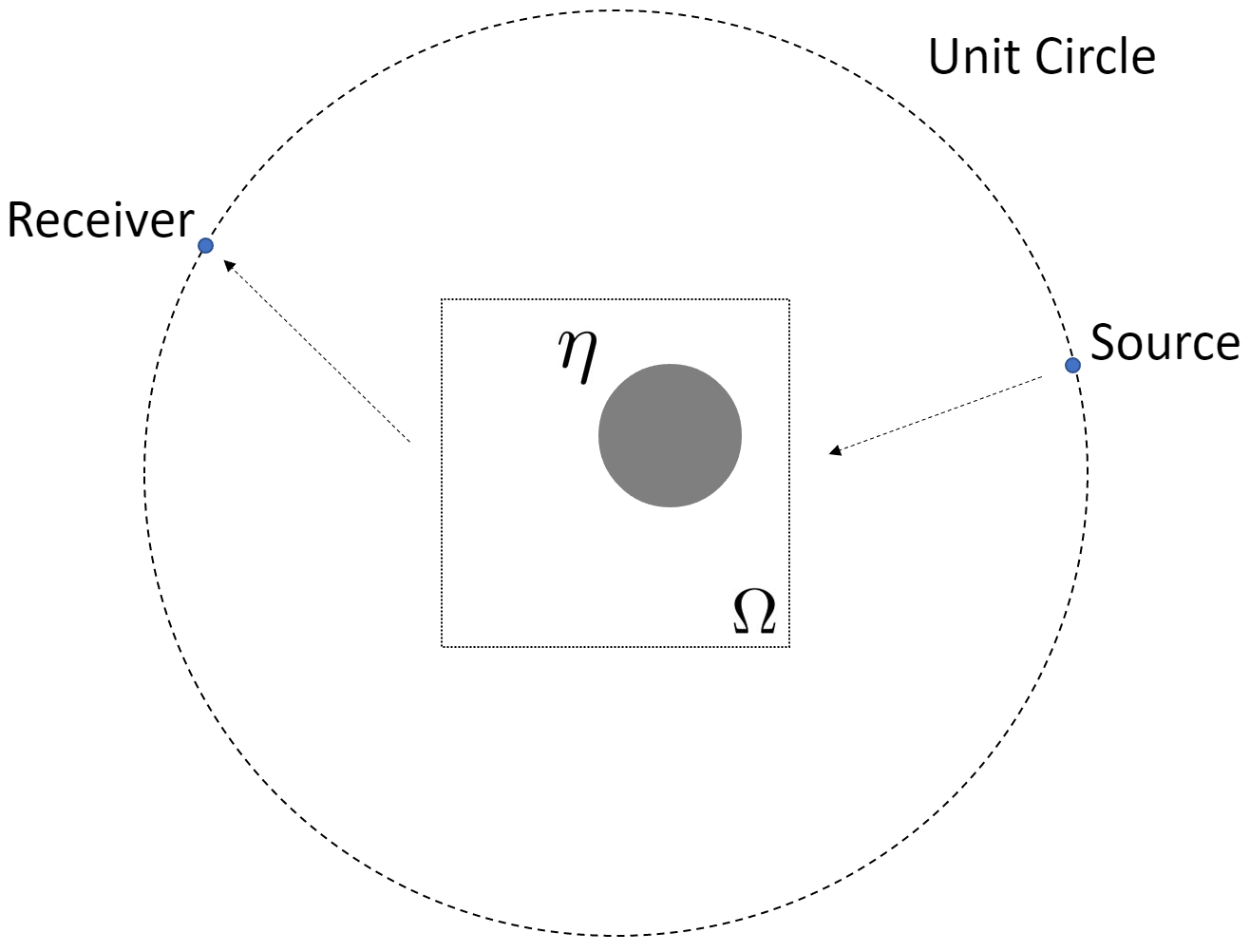
Figure 1: The data generating process for the far-field pattern problem.

The exact form of the far-field data $u_{\sigma_{1}}^{\infty}$ can be derived under the general framework of (1). Consider a source located at a position $-\sigma_{1}\rho$, where $\sigma_{1}$ is a direction and $\rho$ is a distance going to infinity. The source magnitude is required to scale up by $\sqrt{\rho}e^{-i\omega\rho}$ to compensate for the spreading of the wave field and the phase shift (see for example Khoo and Ying (2019)). In the limit of $\rho\rightarrow\infty$, we have

$$\begin{split}&\lim_{\rho\rightarrow\infty}\left(G_{0}\Pi_{\Sigma}\right)(\sigma_{1},x)\\ =&\lim_{\rho\rightarrow\infty}(1/\sqrt{\rho})e^{i\omega|x-(-\sigma_{1}\rho)|}\sqrt{\rho}e^{-i\omega\rho}\\ =&\lim_{\rho\rightarrow\infty}(1/\sqrt{\rho})e^{i\omega(\rho+\sigma_{1}\cdot x)}\sqrt{\rho}e^{-i\omega\rho}\\ =&e^{i\omega\sigma_{1}\cdot x}.\end{split}$$

The same setup works in the prescription of receivers. Suppose a receiver is located at a position $\sigma_{2}\rho^{\prime}$, where $\sigma_{2}$ is a direction and $\rho^{\prime}$ is a distance going to infinity. Then we have

$$\begin{split}&\lim_{\rho^{\prime}\rightarrow\infty}\left(\Pi_{\mathcal{R}}G_{0}\right)(x,\sigma_{2})\\ =&\lim_{\rho^{\prime}\rightarrow\infty}\left(1/\sqrt{\rho^{\prime}}\right)e^{i\omega\left|\sigma_{2}\rho^{\prime}-x\right|}\sqrt{\rho^{\prime}}e^{-i\omega\rho^{\prime}}\\ =&\lim_{\rho^{\prime}\rightarrow\infty}\left(1/\sqrt{\rho^{\prime}}\right)e^{i\omega\left(\rho^{\prime}-\sigma_{2}\cdot x\right)}\sqrt{\rho^{\prime}}e^{-i\omega\rho^{\prime}}\\ =&e^{-i\omega\sigma_{2}\cdot x}.\end{split}$$

Combining the above two limiting processes together, the observed data $d(\sigma_{1},\sigma_{2})$ for a source at a location $\sigma_{1}$ and a receiver at a location $\sigma_{2}$ can be computed as follows in the sense of limit:

$$d(\sigma_{1},\sigma_{2})=\sum_{x\in X}\sum_{y\in X}e^{-i\omega\sigma_{2}\cdot x}\left(E+EG_{0}E+\cdots\right)(x,y)e^{i\omega\sigma_{1}\cdot y},$$ (3)

where $\omega$ is the frequency of the wave field from the source at the location $\sigma_{1}$. As mentioned previously, we approximate (3) as a polynomial in $E$ up to $k$-th order. For simplicity, we write (3) succinctly as:

$$d(\sigma_{1},\sigma_{2})=F_{\omega,\mathcal{R},\Sigma}(\eta)(\sigma_{1},\sigma_{2}).$$ (4)

Besides the far-field pattern, another widely used setting called seismic imaging is also considered in our paper.

2.3 Seismic Imaging

In seismic imaging, the domain $\Omega$ is rectangular with Sommerfeld radiation boundary condition specified and all sensors can only be installed on a single line parallel to an edge of $\Omega$. The data generation process of seismic imaging is shown in Figure 2. The sources and receivers are well separated from the scatterer $\eta$.

The operators in (1) can be written simply as:

$$(\Pi_{\mathcal{R}}G_{0})(x,\sigma)=G_{0}(x,\sigma)$$ (5)

$$(G_{0}\Pi_{\Sigma})(\sigma,x)=G_{0}(\sigma,x)$$ (6)

Then the observed data $d(\sigma_{1},\sigma_{2})$ for a source at a location $\sigma_{1}$ and a receiver at a location $\sigma_{2}$ can be computed as follows:

$$d(\sigma_{1},\sigma_{2})=\sum_{x\in X}\sum_{y\in X}G_{0}(\sigma_{2},x)\left(E+EG_{0}E+\cdots\right)(x,y)G_{0}(\sigma_{1},y),$$ (7)

where $\omega$ is the frequency of the wave field from the source at the location $\sigma_{1}$. For simplicity, we also use (4) to represent (7) in seismic imaging setting.

Figure 2: The data generating process for the seismic imaging problem.

In the next section, based on the forward model (3), we introduce the proposed reinforcement learning scheme to solve the inverse problem.

3 Reinforcement Learning Framework for Inverse Scattering

In the typical data collection of inverse scattering, sensors are either installed randomly or uniformly on the unit circle. Moreover, wave frequencies are empirically selected. To achieve a better reconstruction quality and stability, reinforcement learning is applied in this paper to learn a strategy that adaptively decides sensor angles and wave frequencies in a sequential manner: 1) several sets of sensors and frequencies are set up sequentially; 2) the locations of sensors and the frequencies of waves are decided according to the reconstruction result based on previous results. This is a sequential decision process that gradually adjusts data collection to obtain better reconstructions, and furthermore, this method uses individualized strategies for imaging different $\eta$’s.

The rest of the section is organized as follows. In section $3.1$, we introduce the problem setting, which establishes the foundation for the following sections. In section $3.2$, we describe the MDP formulation of the problem, which enables us to use RL methods to solve it. In section $3.3$, we review some basic notions and methods in RL, and introduce the RL algorithm we used to optimize the policy in the MDP described in section $3.2$. In section $3.4$, we introduce the solver used in scatterer reconstruction, which is required in RL algorithms in section $3.3$. In section $3.5$ and section $3.6$, we present the structure of the policy network and the value network. In section $3.7$ and section $3.8$, we explain the training procedure and test procedure of our RL model, combining all the sections from $3.1$ to $3.7$.

3.1 Problem Setting

Without loss of generality, we assume that the true scatterer $\eta(x)$ is compactly supported in a unit square $\Omega$ centered at the origin, and all the probes are placed on the unit circle in $\mathbb{R}^{2}$ (containing $\Omega$). In a reinforcement learning framework as we describe later, an action $a_{t}$ decides the location of sensors and the choice of frequencies at time $t$. In this case, we discretize the unit sphere $\mathbb{S}^{1}$ uniformly and define $\sigma^{a_{t}}\in\mathbb{R}^{360}$ as an indicator vector to specify the location of one sensor. $\sigma^{a_{t}}$ has only one non-zero entry to indicate the angle of the sensor on a unit sphere $\mathbb{S}^{1}$. In the experiment, we place one sensor on the unit circle in each step until $T$ sensors have been placed, where $T$ is a number decided by user in advance. In each step, sensors send out incident waves and receive scattered waves. At time $t$, given a group of sensors placed sequentially at $\sigma^{a_{i}}$ $(i=1,2,\ldots,t-1)$, a new sensor $\sigma^{a_{t}}$ is added on the unit circle. A wave field of frequency $\omega^{a_{t}}$ is launched from this new sensor and transmits through the domain $\Omega$. Then sensors at $\sigma^{a_{1}},\ldots,\sigma^{a_{t}}$ will receive the scattered wave. Each sensor is not only a source but also a receiver. We denote the receiver set at time $t$ as $\mathcal{R}^{a_{t}}$ and the source set at time $t$ as $\Sigma^{a_{t}}$. Therefore, $\mathcal{R}^{a_{t}}=\{\sigma^{a_{1}},\ldots,\sigma^{a_{t}}\}$ and $\Sigma^{a_{t}}=\{\sigma^{a_{t}}\}$. We also assume the observed data at time $t$ can be approximated by (4): $d_{t}=F_{\omega^{a_{t-1}},\mathcal{R}^{a_{t-1}},\Sigma^{a_{t-1}}}(\eta)$. It is important to emphasize that that the frequency $\omega^{a_{t}}$ at step $t$ can be different from others. After $T$ steps, the data collection procedure ends and we will reconstruct the scatterer $\eta$ with all the measurements recorded. We define the entire data collection procedure as an episode and this episode consists of $T$ sequential steps. The goal of this paper is to improve the reconstruction quality while limiting the number of probes to use. Our solution is to learn an optimal strategy for data collection.
The original problem of determining sensor location and wave frequency is a combinatorial optimization problem and is NP-hard. We’ll formulate the problem as a Markov Decision Process (MDP) in section $3.2$, which can be further solved by reinforcement learning methods.

3.2 Markov Decision Process Formulation

The procedure of deciding sensor locations and frequency values in inverse scattering is a sequential decision problem, where one needs to make a choice of angle and frequency at each step. Thus it can be formulated as a Markov Decision Process (MDP). In this way, we can use RL to solve the problem efficiently. We now elaborate how to formulate our problem as an MDP:

1. State at time $t$ is $s_{t}=(I_{1},I_{2},\ldots,I_{t})$, where $I_{t}=(d_{t},u_{t},T+1-t)$. The first term $d_{t}=F_{\omega^{a_{t-1}}\mathcal{R}^{a_{t-1}},\Sigma^{a_{t-1}}}(\eta)\in\mathbb{C}^{1\times(t-1)}$ is the collected observation data at step $t$. The size $1\times(t-1)$ comes from the fact that at time $t$, we send out wave from a single source to $t-1$ receivers. Measurements up to time $t$ are all included in state $s_{t}$ because the reconstruction at step $t$ relies on all the previous collected data. The second term $u_{t}\in\mathbb{R}^{360}$ is a vector recording all the angles where sensors have already been placed by time $t$ and the corresponding wave frequencies. The $j$-th entry of $u_{t}$ denotes the angle $\frac{2j\pi}{360}$. If the $j$-th angle is selected at any step $k$ $(k\leq t)$, then the $j$-th entry of $u_{t}$ is $\omega^{a_{k}}$, denoting the frequency of the wave sent at $k$-th step. If no wave is sent from a specific angle, the entry in $u_{t}$ corresponds to that angle is $0$. The last term $T+1-t$ means the number of sensors left to be placed.

2. Action taken at time $t$ is $a_{t}$. It is used to define choices on angles and frequencies $\sigma^{a_{t}}$ and $\omega^{a_{t}}$. $\sigma^{a_{t}}\in\mathbb{R}^{360}$ is a one-hot vector which denotes the angle of the new sensor to be added at time $t$. $\omega^{a_{t}}\in\mathbb{R}$ stands for the frequency of its incident wave. In particular, $u_{t}$ can be defined in terms of $\sigma^{a_{t}}$ and $\omega^{a_{t}}$ as $u_{t}=\sum_{j=1}^{t-1}\omega^{a_{j}}\sigma^{a_{j}}$.

3. Transition model. State $s_{t}$ and action $a_{t}$ enable us to compute a deterministic $s_{t+1}$ under a noise-free model. According to (4), the new measurement $d_{t+1}=F_{\omega^{a_{t}},\mathcal{R}^{a_{t}},\Sigma^{a_{t}}}(\eta)$ can be computed given $s_{t}$ and $a_{t}$. Meanwhile, $u_{t+1}=u_{t}+\omega^{a_{t}}\sigma^{a_{t}}$. Therefore, $I_{t+1}=(d_{t+1},u_{t+1},T-t)$ and the new state $s_{t+1}=(I_{1},\ldots,I_{t+1})$.

4. Reward at time $t$ is $r_{t}$, which is defined as the increment in the Peak Signal to Noise Ratio (PSNR) value of the reconstruction compared to last step. PSNR is commonly used to quantify reconstruction quality for images. We apply its increment here to quantify how much the new reconstruction has been improved due to the new action. Suppose the reconstruction at step $t$ is $\hat{\eta}_{t}$ and the true scatterer is $\eta$, then $r_{t}=\text{PSNR}(\hat{\eta}_{t},\eta)-\text{PSNR}(\hat{\eta}_{t-1},\eta)$. In this paper, $\eta$ is reconstructed by a regularization-based optimization method to be introduced later. We would like to point out that better results might be possible if more sophisticated reconstruction methods were used.

When we do not know the transition probability, we need a reinforcement learning framework to simultaneously learn the action taken and the transition probability.

3.3 Reinforcement Learning Algorithm

In RL, an agent interacts with environment to obtain a sequence of data, based on which the agent learns a policy to maximize a certain accumulated reward to finish a task. Given an interaction trajectory between agent and environment $\tau=(s_{1},a_{1},r_{1},s_{2},a_{2},r_{2},\ldots)$, the total reward over time is

$$G(\tau)=r_{1}+\gamma r_{2}+\gamma^{2}r_{3}+\ldots,$$

where $\gamma\in[0,1]$ is a discount rate. We use $\gamma=1$ since the reward at each step is of equal importance in our application. The policy in the MDP is defined as the conditional probability $\pi(a|s)$ for $a_{t}=a$ and $s_{t}=s$. $\pi(a|s)$ denotes the probability of taking action $a$ at step $t$ while the state is $s$. The value function of a state $s$ following a certain policy $\pi$ is given as

$$v_{\pi}(s)=\mathbb{E}_{\tau}[r_{1}+\gamma r_{2}+\gamma^{2}r_{3}+\ldots|s_{1}=s,\tau\sim\pi].$$

Similarly, the value function of a state-action pair $(s,a)$ is defined as

$$q_{\pi}(s,a)=\mathbb{E}_{\tau}[r_{1}+\gamma r_{2}+\gamma^{2}r_{3}+\ldots|s_{1}=s,a_{1}=a,\tau\sim\pi].$$

In an MDP, the RL algorithm aims to find an optimal policy that maximize the expected value of initial state $s_{1}$ following a probability distribution $p(s)$:

$$\max\limits_{\pi}\mathbb{E}_{s_{1}\sim p(s)}[v_{\pi}(s_{1})].$$

Currently, model-free RL algorithms mainly fall into two categories: value-based methods and policy-based methods. Value-based algorithms learn the state or state-action value and act by choosing the best action in the state, which requires comprehensive exploration. For example, Q-learning (Watkins and Dayan, 1992) learns the optimal Q function through the Bellman Equation and chooses a greedy action, which maximize the learned Q function. Since the maximization requires searching on the action space, it will become slow and imprecise if the actions are continuous. This means that value-based algorithms are more suitable for discrete actions. On the other hand, policy gradient methods (Sutton et al., 1999; Silver et al., 2014) are more suitable for continuous actions because they directly optimize a parameterized policy under a surrogate objective. Though the variables (angles and frequencies) in our current setting are discrete, we adopt the policy-based method for possible future extensions to continuous cases.

More specifically, we use policy gradient methods that directly optimize a policy $\pi_{\theta}$ (parameterized by a neural network) under a certain objective function. Policy gradient methods seek to maximize the performance of $\pi_{\theta}$ via stochastic updates, whose expectation approximates the gradient of the performance measure with respect to $\theta$. In our experiments, we use the Proximal Policy Optimization (PPO) algorithm (Schulman et al., 2017). Given an old policy $\pi_{\theta_{\text{old}}}$ and a new policy $\pi_{\theta}$, let $\gamma_{\theta}$ denote the probability ratio $\gamma_{\theta}(s,a)=\frac{\pi_{\theta}\left(a\mid s\right)}{\pi_{\theta_{\text{old }}}\left(a\mid s\right)}$. An advantage function of policy $\pi_{\theta}$ is introduced as

$$\alpha_{\pi_{\theta}}(s,a)=q_{\pi_{\theta}}(s,a)-v_{\pi_{\theta}}(s).$$ (8)

The objective function to optimize is then defined as:

$$L^{\operatorname{clip}}(\theta)=\mathbb{E}_{s,a\sim\pi_{\theta_{\text{old}}}}\left[\min\left(\gamma_{\theta}(s,a)\alpha_{\pi_{\theta_{\text{old}}}}(s,a),\operatorname{clip}\left(\gamma_{\theta}(s,a),1-\epsilon,1+\epsilon\right)\alpha_{\pi_{\theta_{\text{old}}}}(s,a)\right)\right],$$

where $\epsilon$ is a hyperparameter and $\text{clip}(x,y,z)=\min(\max(x,y),z)$. This method employs clipping to avoid destructively large policy updates, which retains the stability and reliability of trust-region methods but is much simpler to implement in practice.

In the MDP, a reward needs to be computed each step. This means that we need to generate a reconstruction of the scatterer each step because of our choice of the reward.

3.4 Reconstruction

According to (4), for a choice of frequency $\omega^{a_{t}}$, receiver set $\mathcal{R}^{a_{t}}$ and source set $\Sigma^{a_{t}}$ at step $t$, the approximate measurement $d_{t+1}$ is given by

$$d_{t+1}=F_{\omega^{a_{t}},\mathcal{R}^{a_{t}},\Sigma^{a_{t}}}(\eta),$$

where $\eta$ is the true scatterer. We reconstruct $\eta(x)$ by minimizing an $\ell_{2}$ loss of data discrepancy with an $\ell_{1}$ penalization to encourage sparsity:

$$\min_{\hat{\eta}}\ \|d-F_{\omega,\mathcal{R},\Sigma}(\hat{\eta})\|_{2}^{2}+\lambda\|\hat{\eta}\|_{1},$$

where $\lambda>0$ is a hyperparameter. Due to the small number of measurements, we observe that the use of a regularization like $\ell_{1}$ significantly improve the results. A new reconstruction is generated at each step in order to compute a reward of the RL model. Given state $s_{t}$ and action $a_{t}$, the reconstruction $\hat{\eta}_{t}$ obtained at time $t$ is:

$$\begin{aligned} \hat{\eta}_{t}&=\underset{\hat{\eta}}{\text{argmin}}\ \sum\limits_{i=1}^{t}\|d_{i+1}-F_{\omega^{a_{i}},\mathcal{R}^{a_{i}},\Sigma^{a_{i}}}(\hat{\eta})\|_{2}^{2}+\lambda\|\hat{\eta}\|_{1}\\ &\coloneqq g(s_{t},a_{t}),\end{aligned}$$ (9)

which has taken the advantage of all the previously collected measurements.

In our numerical experiment, $\lambda$ is set to be $0.1$ and L-BFGS Gao et al. (2022) is used to solve the optimization problem in (9) for the reconstruction problem at each step. Given an initialization $\hat{\eta}$, we perform L-BFGS for $3$ iterations to obtain the reconstruction of the current step. It is important to point out that warm start is necessary to obtain good results. In our tests, we use the reconstruction result of the last step as the initialization of the current step. This greatly reduces the computational cost and ensures convergence.

In the previous sections, we formulate the original problem as an MDP and introduce how to compute the terms in the MDP. In order to apply policy gradient methods, we need to build a policy network that parameterizes the policy to learn.

3.5 Policy Network

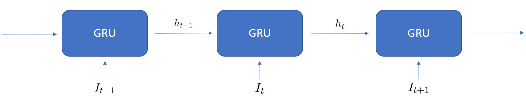
Figure 3: Structure of Recurrent Neural Network. Each GRU represents one layer, $I_{t}$ is the input of layer $t$. Each layer outputs a hidden state $h_{t}$ which is also the input of next layer.

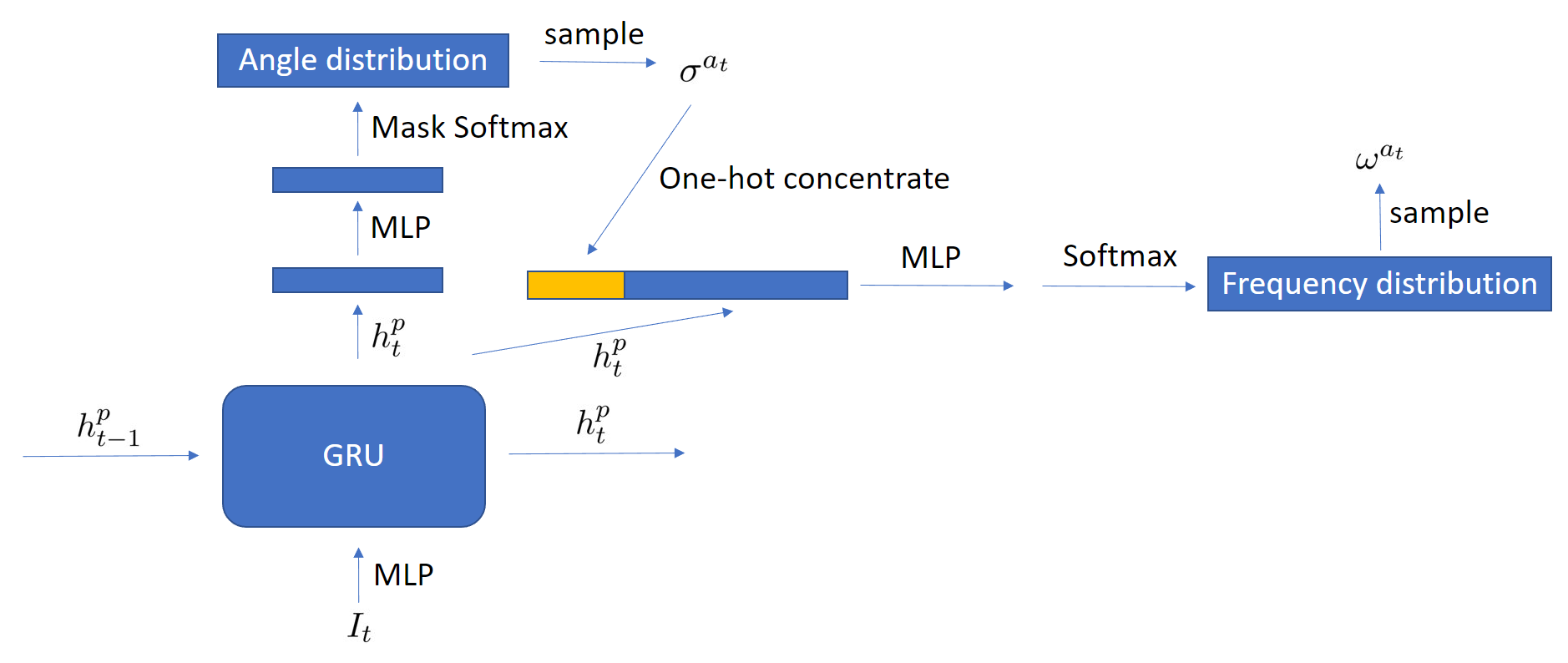
Figure 4: Structure of policy network $\pi_{\theta_{p}}$. $h_{t}^{p}$ represents the hidden state of policy net, which is the output of GRU at layer $t$. $I_{t}=(d_{t},u_{t},T+1-t)$. We use $h_{t}^{p}$ as the input of another perceptron and generate a 360-dim categorical distribution of angle through softmax function with a mask removing angles that have been chosen. This distribution is the angle policy $\pi_{\theta_{p}}^{\sigma}$. Then we randomly generate an angle $\sigma^{a_{t}}$ based on distribution and combine its one-hot concentrate with $h_{t}^{p}$ as the input of another MLP, which gives rise to another categorical distribution of frequency. This distribution represents the frequency policy given angle $\pi_{\theta_{p}}^{\omega|\sigma}$. Finally, we use this to randomly generate a frequency $\omega^{a_{t}}$.

In order to handle the increasing dimension of state $s_{t}$ over time, we use a Recurrent Neural Network (RNN) to parameterize the policy. The specific structure of RNN enables us to store all the past information in $s_{t}$ in a hidden state while adding new information at each step. More specifically, we use multi-layer Gated Recurrent Units (GRU), which was introduced in 2014 by (Chung et al., 2014) and also applied in Shen et al. (2020). It is similar to a long short-term memory (LSTM) with fewer parameters. The structure of the whole GRU is shown in Figure 3. The policy network is denoted by $\pi_{\theta_{p}}$, where $\theta_{p}$ represents the training parameters. We use $h_{t}^{p}$ to represent the output of the policy network at layer $t$, which is called a hidden state. First, a multi-layer perceptron (MLP) is used to extract features from an input $I_{t}=(d_{t},u_{t},T+1-t)$. Then, the features and the output of GRU in the last layer (a hidden state $h_{t-1}^{p}$) are processed by a GRU. In order to learn the sensor angle, the output of GRU will be further processed by another MLP. This MLP aims to learn the policy for angle based on the information from state $s_{t}$. With the help of a softmax function, its output is turned into a categorical distribution of angles (a 360-dimensional vector). The value at each entry denotes the possibility of placing a sensor at the corresponding angle. Because an angle cannot be chosen more than once in one episode, a mask is introduced to remove all the previously chosen angles. This angle distribution is denoted by $\pi_{\theta_{p}}^{\sigma}$, which represents the policy for angle $\sigma$. During training, an angle is sampled based on the distribution $\pi_{\theta_{p}}^{\sigma}$, which is further used to generate a one-hot 360-dimensional vector. This vector uses $1$ to denote the chosen angle and 0 otherwise. After that, the output of GRU $h_{t}^{p}$ and the selected angle $\sigma^{a_{t}}$ are merged into a single vector, which is used to learn the frequency policy. This is because the wave frequency should depend not only on state $s_{t}$ but also on chosen angle $\sigma^{a_{t}}$. In our experiment, the frequency can only be chosen from $4$ given values. So the merged vector is processed by another MLP with an output as a $4$-dimensional vector, which denotes the categorical distribution of frequencies. We denote this distribution as $\pi_{\theta_{p}}^{\omega|\sigma}$ emphasizing that the policy of frequency $\omega$ depends on angle $\sigma$. Finally, a random frequency is sampled from the distribution $\pi_{\theta_{p}}^{\omega|\sigma}$. The structure of the policy network is shown in Figure 4. To conclude, the policy network learns the policy $\pi_{\theta_{p}}(a|s)$ of an action given a state, which consists of an angle policy $\pi_{\theta_{p}}^{\sigma}$ and a frequency policy $\pi_{\theta_{p}}^{\omega|\sigma}$. The angles and frequencies generated by policy nets during training are random samples from these two distributions.

Besides the policy network, a value network is required for training in policy gradient methods.

3.6 Value Network

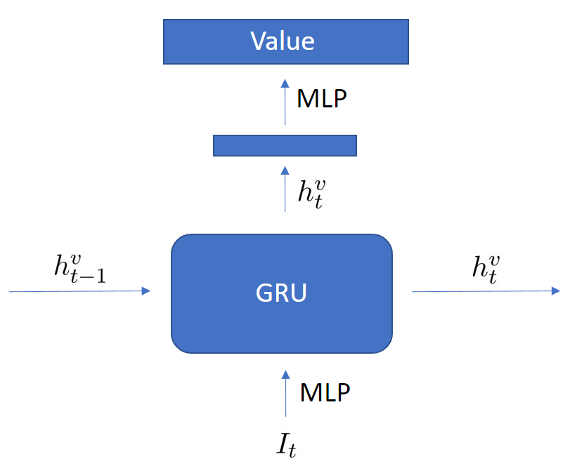
Figure 5: Structure of value network $\gamma_{\theta_{v}}$. $h_{t}^{v}$ represents the hidden state of value net, which is the output of GRU at layer $t$. $I_{t}=(d_{t},u_{t},T+1-t)$. We use $h_{t}^{v}$ as the input of another perceptron and generate $\hat{v}_{\pi_{\theta_{p}}}(s_{t})$, which is the estimate of the value of current state $s_{t}$ under the policy $\pi_{\theta_{p}}$ parameterized by policy network.

In addition to the policy network, we also build a value network $\gamma_{\theta_{v}}$ parametrized by trainable parameters $\theta_{v}$ with a similar structure as in the policy network to approximate the value function of states. The value function approximation is required in the evaluation of the advantage function of policy $\pi_{\theta}$ in (8). The value network design is visualized in Figure 5. We use $h_{t}^{v}$ to represent the output of the value network after the $t$-th layer. At the $t$-th step, an MLP is used to extract features from the current input $I_{t}=(d_{t},u_{t},T+1-t)$. Then, the features of $I_{t}=(d_{t},u_{t},T+1-t)$ and the output of GRU in previous step (a hidden state $h_{t-1}^{v}$) are processed by a GRU to generate $h_{t}^{v}$. The difference between the policy network and the value network is how they process $h_{t}^{v}$ to generate useful information. The output $h_{t}^{v}$ of a GRU in the value network is processed by an MLP to generate a deterministic estimate of the value function $v_{\pi_{\theta_{p}}}(s)$, instead of a distribution in the policy network. The estimated value of a state given by the value network is denoted by $\hat{v}_{\pi_{\theta_{p}}}(s)$.

With the policy network and the value network, we can train the RL model through policy gradient methods.

3.7 Training Procedure

Now we will introduce the training procedure of the policy network $\pi_{\theta_{p}}$ and the value network $\gamma_{\theta_{v}}$. The training set consists of a specific type of scatterers randomly generated. A scatterer $\eta$ will be randomly chosen from the training set and used to generate an interaction trajectory of the RL model $\tau=(s_{1},a_{1},r_{1},\ldots,s_{T},a_{T},r_{T})$. In the initialization of the episode, we set $d_{1}=0$, $u_{1}=0$ and $h_{1}^{p}=h_{1}^{v}=0$. Thus the initial state $s_{1}=I_{1}=(d_{1},u_{1},T)$. At step $t$, given past information $h_{t-1}^{p}$ and current information $I_{t}$, the policy network learns a policy $\pi_{\theta_{p}}(a_{t}|s_{t})$. Meanwhile, the value network approximates the value of state $s_{t}$ under the current policy $\hat{v}_{\pi_{\theta_{p}}}(s_{t})$. During training, angles and frequencies are randomly sampled based on the policy $\pi_{\theta_{p}}(a_{t}|s_{t})$. In this way, a more comprehensive exploration of the action space is encouraged for faster convergence. A new sensor is then placed at angle $\sigma^{a_{t}}$ to launch an incident wave of frequency $\omega^{a_{t}}$. So the receiver set is $\mathcal{R}^{a_{t}}=\{\sigma^{a_{1}},\ldots,\sigma^{a_{t}}\}$ and the sensor set is $\Sigma^{a_{t}}=\{\sigma^{a_{t}}\}$ at step $t$. Based on the formula in (4), a new measurement $d_{t+1}=F_{\omega^{a_{t}},\mathcal{R}^{a_{t}},\Sigma^{a_{t}}}(\eta)$ is obtained. Meanwhile, compute $u_{t+1}=u_{t}+\omega^{a_{t}}\sigma^{a_{t}}$ and let $s_{t+1}=(d_{t+1},u_{t+1},T-t)$. Then the reconstruction $\hat{\eta}_{t}$ at time $t$ is computed based on all the previously collected measurements. Let us denote $\hat{\eta}_{t}$ explicitly as $\hat{\eta}_{t}=g(s_{t},a_{t})$ according to (9). In this way, we can compute the reward $r_{t}$ as the increment in the PSNR of the reconstruction: $r_{t}=\text{PSNR}(\hat{\eta}_{t},\eta)-\text{PSNR}(\hat{\eta}_{t-1},\eta)$. When the reward $r_{t}$ and state $s_{t+1}$ are ready, the value network approximates the value $\hat{v}_{\pi_{\theta_{p}}}(s_{t+1})$ in order to estimate the advantage function $\alpha_{\pi_{\theta_{p}}}(s_{t},a_{t})\approx\hat{v}_{\pi_{\theta_{p}}}(s_{t+1})+r_{t}-\hat{v}_{\pi_{\theta_{p}}}(s_{t})$. We denote the estimate of the advantage as $\hat{\alpha}_{\pi_{\theta_{p}}}(s_{t},a_{t})$. These estimates will be used in PPO. The episode ends after $T$ steps and an interaction trajectory $\tau=(s_{1},a_{1},r_{1},\ldots,s_{T},a_{T},r_{T})$ has been generated. In practice, we generate several episodes on parallel and train the policy network and the value network on a mini batch of episodes. Based on these simulations, we can compute the surrogate objective function of PPO and optimize our neural networks. We use auto-differentiation and Adam to optimize the surrogate objective of PPO, and the choice of hyperparameters can be found in Section $4$. A major advantage of using PPO is that we can apply multiple optimization steps using a few trajectories without destructively large policy updates. A more detailed algorithm can be found in Algorithm 1.

After training the RL model on a training set, we need to test the performance of the model on a new test set. The test procedure is a bit different from the training procedure.

3.8 Test Procedure

Given the fully trained policy network $\pi_{\theta_{p}}$, we can test the RL model on a set of scatterers that are similar to those in the training set. During testing, given a scatterer $\eta$ randomly selected from the test set, the policy network generates an interaction trajectory $\tau=(s_{1},a_{1},r_{1},\ldots,s_{T},a_{T},r_{T})$. The initialization is the same as before: $d_{1}=0$, $u_{1}=0$, $h_{0}^{p}=0$ and $\hat{\eta}_{0}=0$. At step $t$, the policy network learns a policy of deciding angles $\pi_{\theta_{p}}^{\sigma}$ and a policy of choosing frequencies $\pi_{\theta_{p}}^{\omega}$ based on the hidden state $h_{t}^{p}$ and the current information $I_{t}=(d_{t},u_{t},T+1-t)$. These policies return probability distributions of angles and frequencies. Note that, in the training of RL, angles and frequencies are randomly chosen according to their probability distributions to encourage the exploration of the action space. However, in the testing of the RL model, we choose the angle and the frequency corresponding to the highest probability, hoping to achieve the highest reconstruction resolution. After deciding an action, a new sensor is placed and the state is updated: $d_{t+1}=F_{\omega^{a_{t}},\mathcal{R}^{a_{t}},\Sigma^{a_{t}}}(\eta)$ and $u_{t+1}=u_{t}+\omega^{a_{t}}\sigma^{a_{t}}$. After $T$ steps, we apply L-BFGS with more iterations (20 iterations) to reconstruct a scatterer via (9) to ensure convergence: $\hat{\eta}_{T}=g(s_{T},a_{T})$. This $\hat{\eta}_{T}$ is the reconstruction of $\eta$ given by the RL model.

1:  Require: A training sample size $k$, randomly generated training scatterer samples $\{\eta_{i}\}_{1\leq i\leq k}$, a grid size $N$, the total number of sensors $T$, a policy network $\pi_{\theta_{p}}$, a value network $\gamma_{\theta_{v}}$, a clipping constant $\epsilon$

2:  For epoch $=0,1,2,\ldots$

3:    Initialization: $d_{1}=0$, $u_{1}=0$, $s_{1}=I_{1}=(d_{1},u_{1},T)$, $h_{0}^{p}=0$, $h_{0}^{v}=0$, $\hat{\eta}_{0}=0$, $\hat{v}_{\pi_{\theta_{p}}}(s_{1})=0$, randomly choose a scatterer $\eta$ from $\{\eta_{i}\}_{1\leq i\leq k}$

4:    For $t=1,\ldots,T$:

5:      Given $h_{t-1}^{p}$ and $I_{t}$, use policy networks to generate policies $\pi_{\theta_{p}}^{\sigma}$ and $\pi_{\theta_{p}}^{\omega|\sigma}$, and then update $h_{t}^{p}$

6:      Randomly sample an angle $\sigma^{a_{t}}$ from the policy $\pi_{\theta_{p}}^{\sigma}$ and a frequency $\omega^{a_{t}}$ from the policy $\pi_{\theta_{p}}^{\omega|\sigma}$

7:      Let $p^{\sigma^{a_{t}}}_{\theta_{p\text{old}}}=\pi_{\theta_{p}}^{\sigma}(\sigma^{a_{t}}|s_{t})$ and $p^{\omega^{a_{t}}}_{\theta_{p\text{old}}}=\pi_{\theta_{p}}^{\omega|\sigma}(\omega^{a_{t}}|\sigma^{a_{t}},s_{t})$

8:      Update the receiver set $\mathcal{R}^{a_{t}}=\{\sigma^{a_{1}},\ldots,\sigma^{a_{t}}\}$ and the source set $\Sigma^{a_{t}}=\{\sigma^{a_{t}}\}$

9:      Compute the state $s_{t+1}$ using $d_{t+1}=F_{\omega^{a_{t}},\mathcal{R}^{a_{t}},\Sigma^{a_{t}}}(\eta)$, $u_{t+1}=u_{t}+\omega^{a_{t}}\sigma^{a_{t}}$, and $I_{t+1}=(d_{t+1},u_{t+1},T-t)$

10:      Given $h_{t-1}^{v}$ and $I_{t}$, use the value network to approximate the value $\hat{v}_{\theta_{p}}(s_{t+1})$, then update $h_{t}^{v}$

11:      Reconstruct a scatterer $\hat{\eta}_{t}=g(s_{t},a_{t})$

12:      Compute the reward $r_{t}=\text{PSNR}(\hat{\eta}_{t},\eta)-\text{PSNR}(\hat{\eta}_{t-1},\eta)$

13:      Approximately compute the advantage function $\hat{\alpha}_{\pi_{\theta_{p\text{old}}}}(s_{t},a_{t})=\hat{v}_{\pi_{\theta_{p}}}(s_{t+1})+r_{t}-\hat{v}_{\pi_{\theta_{p}}}(s_{t})$

14:    End for

15:    Given $h_{0}^{p}$ and $I_{t}$, let $p^{\sigma^{a_{t}}}_{\theta_{p}}$ and $p^{\omega^{a_{t}}}_{\theta_{p}}$ be the probability of the angle $\sigma^{a_{t}}$ and the frequency $\omega^{a_{t}}$ learned by the policy network

16:    Compute $\gamma_{\theta_{p}}(s_{t},a_{t})=\frac{p^{\sigma^{a_{t}}}_{\theta_{p}}p^{\omega^{a_{t}}}_{\theta_{p}}}{p^{\sigma^{a_{t}}}_{\theta_{\text{old}}}p^{\omega^{a_{t}}}_{\theta_{\text{old}}}}$

17:    Evaluate $L^{\operatorname{clip}}(\theta_{p})=\frac{1}{T}\Sigma_{t=1}^{T}(\min(\gamma_{\theta_{p}}(s_{t},a_{t})\hat{\alpha}_{\pi_{\theta_{p\text{old}}}}(s_{t},a_{t}),\text{clip}(\gamma_{\theta_{p}}(s_{t},a_{t}),1-\epsilon,1+\epsilon)\hat{\alpha}_{\pi_{\theta_{p\text{old}}}}(s_{t},a_{t})))$

18:    Given $h_{0}^{v}$ and $I_{t}$, let $\hat{v}_{\theta_{v}}(I_{t})$ be the value approximated by the value network

19:    Evaluate $L(\theta_{v})=\frac{1}{T}\Sigma_{t=1}^{T}(\hat{\alpha}_{\pi_{\theta_{p\text{old}}}}(s_{t},a_{t})+\hat{v}_{\pi_{\theta_{p}}}(s_{t})-\hat{v}_{\theta_{v}}(I_{t}))^{2}$

20:    Use auto-differentiation and Adam to optimize $\theta_{p}$ and $\theta_{v}$ in the objective functions $L^{\operatorname{clip}}(\theta_{p})$ and $L(\theta_{v})$, respectively

21:  End for

22:  Return: The trained policies $\pi_{\theta_{p}}$ and $\gamma_{\theta_{v}}$

Algorithm 1 The Training Procedure of Our Reinforcement Learning Algorithm

4 Numerical Experiment

In this section, we’ll test our model on far field pattern and seismic imaging problem to show its performance.

4.1 Setting

In far field pattern, the scatterer field $\eta(x)$ is discretized at $N\times N$ grid points. $N=32$ or $N=64$ is applied in our numerical results and the numerical conclusion remains similar for other $N$’s. In seismic imaging, the scatterer field is discretized at $N\times 3N$, where $N=32$. In each experiment, we generate $600$ different scatterers, $500$ of which are used for training and the rest are used for testing. The positions of sensors are specified with integer angles in $[0,360)$, while the possible choices for frequencies are $8,16,24,32$ for $N=32$ and $16,32,48,64$ for $N=64$. The meaning of angles is clear in far field pattern. In seismic imaging, we can get a direction for any point on the line where we place sensors, as long as we think of the center of domain $\Omega$ as the origin. If we define the direction of the left endpoint as angle $0$ and the direction of the right endpoint as $360$, then we can assign each point on the line with an angle between $0$ and $360$. Our algorithm allows more choices of frequencies to achieve possible better resolution, but we limit the choices here for computational efficiency. In far field pattern, $10$ probes are applied for sensing when $N=32$ and $15$ are used when $N=64$. In seismic imaging, $6$ probes are used for $N=32$. The choice of $T$ is a user-defined hyper-parameter determined by the requirement of the reconstruction resolution. A larger $T$ leads to a better reconstruction. We assume the measurements in our experiments approximately follow the model in (4) and we take the second-order and third-order models in our numerical tests. As we shall see, our method works well in both nonlinear models and is significantly better than standard sensing methods. The linear model has also been tested and our method also outperforms existing sensing methods. Since the linear case is less interesting than nonlinear cases in practice, only the results of the second and third-order models will be presented here. We use L-BFGS to optimize the objective function in reconstruction, and the model requires a new reconstruction at each step. Only $3$ iterations of L-BFGS are performed and the optimization result is the reconstruction result. Then the result will be the initialization for reconstruction at next step. We set the penalization constant $\lambda$ introduced in Section $3.3$ to be $0.1$.

In the policy network, a multi-layer GRU with $3$ recurrent layers is used and there are $256$ neurons in each layer. The angle MLP has $1$ hidden layer of $512$ neurons and the one for frequency has $2$ hidden layers of $512$ neurons. In the value network, the value MLP is composed of $1$ hidden layer of $512$ neurons. Besides, the MLPs in the policy network and the value network that extract features from $s_{t}$ also contain $2$ hidden layers with $512$ neurons. We use Adam (Kingma and Ba, 2014) to optimize the policy network and value network parameters with a learning rate equal to $0.0004$. and coefficients used for computing running averages of gradient and its square are $\beta_{1}=0.9$ and $\beta_{2}=0.999$. We trained the policy network and the value network with PPO in each experiment for several hundred steps. In each step, we generate $8$ episodes using $8$ scatterers that are randomly chosen from the training set. Then we perform $1$ step of Adam on a mini-batch of $4$ episodes randomly selected from the $8$ scatterers. This action is repeated for $10$ times in a single step mentioned above. The PPO algorithm allows us to repeat the optimization on a few repetitive samples without having destructively large policy updates, thus improving the utilization of data and algorithm efficiency.

We test the numerical results on $5$ different sampling strategies for angles and frequencies. The first one is our reinforcement learning method that learns both angles and frequencies. This method is denoted as “Learn Both". The second one uses random angles with a fixed frequency and, hence, is denoted as “Random Angle". The third one uses uniformly sampled angles with a fixed frequency and, hence, is denoted as “Uniform Angle". The fourth one uses angles learned by the reinforcement learning method while the frequency is fixed and not learned. This method is denoted as “Learn Angle". The fifth method uses a learned frequency from reinforcement learning with random angles. Therefore, this method is denoted as “Learn Frequency". There will be comparative experiments to see the impact of learning angles and frequencies.

For methods that do not learn how to select frequencies, a fixed $\omega$ is used throughout an entire episode. The frequency that reaches the lowest error in the single-frequency case is chosen. During testing, we run L-BFGS for $20$ iterations in the final reconstruction when all the probes have been placed to ensure convergence. To quantify reconstruction accuracy, we use the Mean Squared Error (MSE):

$$\text{MSE}=\frac{1}{N^{2}}\sum_{x\in X}(\eta(x)-\hat{\eta}(x))^{2},$$

and thepeak signal-to-noise ratio (PSNR):

$$\text{PSNR}=20\ \log_{10}(\frac{\text{MAX}_{f}}{\sqrt{\text{MSE}}}),$$

where $\text{MAX}_{f}$ is the maximum possible pixel value of an image. A method is satisfactory if it produces a small MSE or a large PSNR.

4.2 Numerical Results

In conclusion, the RL model that learns both angles and frequencies improves significantly compared to others methods under limited sensing resources. We now explain and present the numerical results of several datasets in detail.

Experiment $1$. (Far field pattern) The size of scatterers is $N=64$ and the measurements come from the second-order model following (4). The scatterers are generated by randomly placing three triangles and three ovals of different sizes in a unit square. The RL model will also work for the third-order model based on results in Experiment $3$, but we only choose the second-order model here to save computational cost. In the second-order model, the norm of the second-order measurement (the second-order term in (4)) is around $\frac{1}{6}$ of the norm of the first-order one. We test this setting because the first-order term should dominate in the expansion. At the same time, the second-order data should not be too small (about one order of magnitude smaller) so that we can verify the power of the RL model in the nonlinear setting. We also test the case where the norm of second-order data is $\frac{1}{2}$ or as large as that of first-order data. The model performs similarly, so we will not present them here.

The policy network and the value network are trained for $400$ steps and $10$ iterations of Adam are performed in each step. After fully trained, the model selects different frequency $\omega$ ranging from $16$ to $48$, while other methods that do not learn frequencies are assigned a fixed frequency of $32$.

We computed the MSE and PSNR of the methods over $50$ test samples randomly selected from the test set. The reconstructions of our model have the smallest error and the largest PSNR among all the $5$ methods on all the $50$ samples. The mean and standard deviation of MSE and PSNR are shown in Table 1. The reconstruction results are visualized in Figure 6. It is clear that learning both angles and frequencies results in a significantly smaller MSE and a larger PSNR than random or uniform angles. Meanwhile, learning both angles and frequencies is also better than learning angles only or learning frequencies only. Our results have demonstrated the effectiveness and necessity of training both angles and frequencies. Meanwhile, the significantly lower variance of MSE demonstrates a better stability of our algorithm than others.

	Learn Both	Random Angle	Uniform Angle	Learn Angle	Learn Frequency
MSE mean (std)	7.6e-5 (1.2e-10)	0.0008 (1.3e-7)	0.0012 (2.8e-7)	0.00015 (6e-9)	0.0018 (6.2e-7)
PSNR mean (std)	113.4 (0.35)	103.6 (5.2)	101.6 (3.9)	110.7 (3.8)	100 (6.1)

Table 1: The MSE and PSNR and their statistics of five different methods in Experiment $1$.

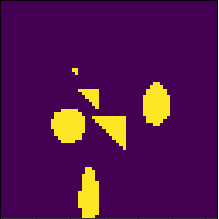
(a) True image

(b) Reconstruction of learning both angles and frequencies (MSE=8e-5)

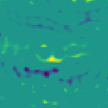
(c) Reconstruction of random angle (MSE=0.0012)

(d) Reconstruction of uniform angle (MSE=0.0017)

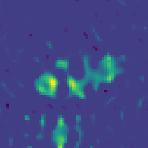
(e) Reconstruction of learning angles only (MSE=3e-4)

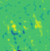
(f) Reconstruction of learning frequencies only (MSE=2e-3)

Figure 6: Experiment $1$. We compare the reconstruction results of the $5$ different methods on a specific type of scatterer. The true scatterer is shown in subplot (a). We tag the methods under each plot, with the MSE of reconstruction showing the difference in resolution.

Experiment $2$. (Far field pattern) The scatterers we used are digital numbers from the MNIST dataset (LeCun et al., 1998) for the purpose of testing different kinds of scatterers. The grid size for discretizing the domain $\Omega$ is $N=28$. The measurements are generated from the second-order model. The RL model is trained for $1000$ steps and it chooses frequency $\omega=7$ for all sensors. The choice of frequencies means that the RL model decides that a single frequency is more suitable than multi-frequencies for this type of scatterers. However, learning frequencies is better than selecting a fixed frequency empirically and mannually because people do not know which frequency will lead to better reconstructions, especially when the number of possible frequencies increases. Since the RL model selects the same frequency for all incident waves, there is no difference between learning both and learning angles only. The same situation holds for sampling angles uniformly and learning frequencies only. So we only compare the performance of learning both angles and frequencies, random angles, and uniform angles in Table 2 and Figure 7. From the table and figure, it is clear that learning both is significantly better than random angles or uniform angles, which demonstrates the necessity of training angles.

	Learn Both	Random Angle	Uniform Angle
MSE mean (std)	0.00012 (8.5e-9)	0.0046 (3e-7)	0.0039 (3.7e-7)
PSNR mean (std)	111.6 (3.3)	95.6 (0.29)	96.29 (0.43)

Table 2: The MSE and PSNR and their statistics of three different methods in Experiment $2$.

Experiment $3$. (Far field pattern) The size of scatterers is $N=32$ and the measurements are generated from the third-order model in (4). We train and test the RL model separately on two types of scatterers. The first type of scatterers is the same as those in Experiment $1$, where scatterers are generated by randomly placing three triangles and three ovals of different sizes in the unit square. The second type of scatterers is generated by randomly placing three circles with different random intensities. The RL model is trained for $1000$ iterations with PPO. The final model sets frequency $\omega$ to be $16$ and $24$ in the first case and chooses $\omega=16$ in the second. Because the second case is simplified to a single-frequency one by the RL model as in Experiment $2$, we will not show the results of learning angles and learning frequencies. The errors are recorded in Table 3 and Table 4. The reconstruction results are visualized in Figure 8. From these results, we can see that the error of learning both angles and frequencies is much smaller than learning angles only, which illustrates the power of training frequencies. The other results are similar to the former two experiments. As shown in Figure 8, the RL model also has the ability to handle different intensities of various objects.

	Learn Both	Random Angle	Uniform Angle	Learn Angle	Learn Frequency
MSE mean (std)	0.0006 (1.2e-8)	0.004 (7e-7)	0.004 (8e-7)	0.0017 (5e-7)	0.011 (7e-6)
PSNR mean (std)	104.3 (0.62)	96.3 (1.4)	96.2 (1.6)	100.7 (4.4)	92.2 (1.2)

Table 3: The MSE and PSNR and their statistics of five different methods on the first type of scatterer in Experiment $3$. The first type of scatterer consists of $3$ randomly placed triangles and $3$ randomly placed ovals with different sizes.

	Learn Both	Random Angle	Uniform Angle
MSE mean (std)	0.0007 (1.4e-8)	0.0045 (9e-7)	0.0053 (4e-7)
PSNR mean (std)	103.6 (0.9)	95.9 (2)	95 (0.5)

Table 4: The MSE and PSNR and their statistics of three different methods on the second type of scatterer in Experiment $3$. The second type of scatterer consists of $3$ randomly placed circles with random intensities.

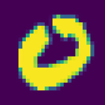
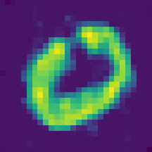
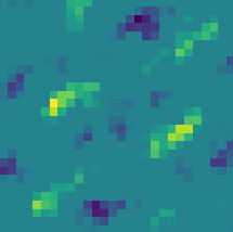
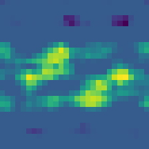
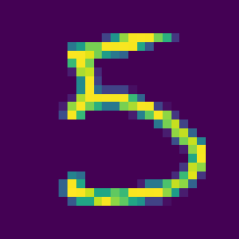
(a) True image

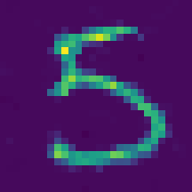
(b) Reconstruction of learning both angles and frequencies (MSE=2e-4)

(c) Reconstruction of random angle (MSE=5e-3)

(d) Reconstruction of uniform angle (MSE=3e-3)

Figure 7: Experiment $2$. We compare the reconstruction results of the $3$ different methods on a specific type of scatterer. The true scatterer is shown in subplot (a). We tag the methods under each plot, with the MSE of reconstruction showing the difference in resolution.

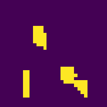
(a) True image

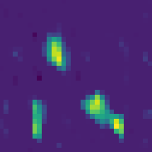
(b) Reconstruction of learning both angles and frequencies (MSE=5e-4)

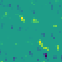
(c) Reconstruction of random angle (MSE=4e-3)

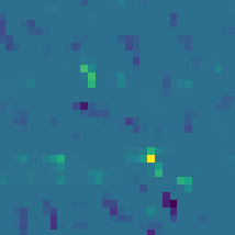
(d) Reconstruction of uniform angle (MSE=5e-3)

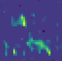
(e) Reconstruction of learning angles only (MSE=2e-3)

(f) Reconstruction of learning frequencies only (MSE=0.01)

(g) True image

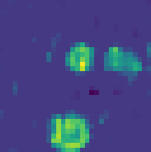
(h) Reconstruction of learning both angles and frequencies (MSE=6e-4)

(i) Reconstruction of random angle (MSE=4e-3)

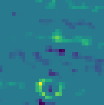
(j) Reconstruction of uniform angle (MSE=4e-3)

Figure 8: Experiment $3$. We compare the reconstruction results of different methods on two different types of scatterers. The true scatterer of the first type is shown in subplot (a). This type of scatterer consists of $3$ randomly placed triangles and $3$ randomly placed ovals with different sizes. The reconstruction results of $5$ different methods are shown in subplot (b) to (f). The true scatterer of the second type is shown in subplot (g). This type of scatterer consists of $3$ randomly placed circles with random intensities. The reconstruction results of $3$ different methods are shown in subplot (h) to (j). We tag the methods under each plot, with the MSE of reconstruction showing the difference in resolution.

Experiment $4$. (Seismic Imaging) In this setting, the domain $\Omega$ is rectangle and all sensors are placed on a horizontal line near the top surface of the domain as in Figure 2.

We consider a domain $\Omega=[-0.5,0.5]\times[-1.5,1.5]$ in the experiment, and the corresponding grid size is $32\times 96$.

We placed $6$ sensors in all and tested the model on second-order and third-order cases. The model works for both cases and we present the results of the third-order case here. The model is trained for 1000 iterations and the final model chooses frequencies to be $8$ and $16$. The results are shown in Table 5 and Figure 9.

	Learn Both	Random Angle	Uniform Angle	Learn Angle	Learn Frequency
MSE mean (std)	4.3e-5 (4e-11)	6.3e-5 (1.5e-10)	5.5e-5 (3e-11)	5e-5 (5e-11)	5.8e-5 (4.5e-11)
PSNR mean (std)	115.9 (0.3)	114.4 (0.9)	114.8 (0.2)	115.2 (0.6)	114.6 (0.4)

Table 5: The MSE and PSNR and their statistics of five different methods in Experiment $4$.

(a) True image

(b) Reconstruction of learning both angles and frequencies (MSE=3.8e-5)

(c) Reconstruction of random angle (MSE=6e-5)

(d) Reconstruction of uniform angle (MSE=4.5e-5)

(e) Reconstruction of learning angles only (MSE=4e-5)

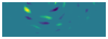
(f) Reconstruction of learning frequencies only (MSE=6.1e-5)

Figure 9: Experiment $4$. We compare the reconstruction results of the $5$ different methods on a specific type of scatterer. The true scatterer is shown in subplot (a). We tag the methods under each plot, with the MSE of reconstruction showing the difference in resolution.

From the results above, we can see that the RL method achieves lower error mean and variance than the other methods in seismic imaging, where the data generation and sensor positions are very different from the far field pattern.

The numerical results show that learning both angles and frequencies achieves the highest resolution with a significant improvement over other methods. Meanwhile, the variance of error indicates that the stability of the RL algorithm is also much better than other methods. Learning angles only is the second-best method and it can generate a vague reconstruction. The difference between the best two methods demonstrates the effectiveness of training frequencies. Sampling angles randomly performs close to sampling uniformly and they are much worse than the previous two methods. This implies that learning angles is necessary for data collection. The performance of learning frequencies only is the worst, which means that the learned frequencies must work together with the learned angles. The numerical results demonstrate the necessity of training sensor angles and incident wave frequencies. Thus, the proposed RL model outperforms all the other methods.

5 Discussion

In this paper, reinforcement learning is applied to learn a policy that selects scatterer-dependent sensing angles and frequencies in inverse scattering. The process of sensor installation, information collection, and scatterer reconstruction is reformulated as a Markov decision process and hence, reinforcement learning can help to optimize this process. A recurrent neural network is adopted as the policy network to choose sensor locations and wave frequencies adaptively. The proposed reinforcement learning method learns to make scatterer-dependent decisions from previous imaging results, each of which requires the solution of an expensive optimization problem. To better facilitate the convergence and reduce the computational cost of reinforcement learning, a warm-start strategy is used in these optimization problems. Extensive numerical experiments have been conducted using several types of scatterers in the second and the third order of the nonlinear inverse scattering model. These results demonstrate that the proposed method significantly outperforms existing algorithms in terms of reconstruction quality. This paper serves as a first step towards intelligent computing for precision imaging in inverse scattering. The case of weak scattering is adopted as a proof of concept. In the future, more advanced learning techniques will be proposed to deal with more challenging cases.

References

- He et al. [2016] Kaiming He, Xiangyu Zhang, Shaoqing Ren, and Jian Sun. Deep residual learning for image recognition. In Proceedings of the IEEE conference on computer vision and pattern recognition, pages 770–778, 2016.
- Silver et al. [2016] David Silver, Aja Huang, Chris J Maddison, Arthur Guez, Laurent Sifre, George Van Den Driessche, Julian Schrittwieser, Ioannis Antonoglou, Veda Panneershelvam, Marc Lanctot, et al. Mastering the game of go with deep neural networks and tree search. nature, 529(7587):484–489, 2016.
- Vinyals et al. [2019] Oriol Vinyals, Igor Babuschkin, Wojciech M Czarnecki, Michaël Mathieu, Andrew Dudzik, Junyoung Chung, David H Choi, Richard Powell, Timo Ewalds, Petko Georgiev, et al. Grandmaster level in starcraft ii using multi-agent reinforcement learning. Nature, 575(7782):350–354, 2019.
- Oord et al. [2016] Aaron van den Oord, Sander Dieleman, Heiga Zen, Karen Simonyan, Oriol Vinyals, Alex Graves, Nal Kalchbrenner, Andrew Senior, and Koray Kavukcuoglu. Wavenet: A generative model for raw audio. arXiv preprint arXiv:1609.03499, 2016.
- Jumper et al. [2021] John Jumper, Richard Evans, Alexander Pritzel, Tim Green, Michael Figurnov, Olaf Ronneberger, Kathryn Tunyasuvunakool, Russ Bates, Augustin Žídek, Anna Potapenko, et al. Highly accurate protein structure prediction with alphafold. Nature, 596(7873):583–589, 2021.
- Shang et al. [2021] Ke Shang, Yunjun Yao, Shunlin Liang, Yuhu Zhang, Joshua B Fisher, Jiquan Chen, Shaomin Liu, Ziwei Xu, Yuan Zhang, Kun Jia, et al. Dnn-met: A deep neural networks method to integrate satellite-derived evapotranspiration products, eddy covariance observations and ancillary information. Agricultural and Forest Meteorology, 308:108582, 2021.
- Morello et al. [2014] V Morello, ED Barr, M Bailes, CM Flynn, EF Keane, and W van Straten. Spinn: a straightforward machine learning solution to the pulsar candidate selection problem. Monthly Notices of the Royal Astronomical Society, 443(2):1651–1662, 2014.
- Borden [2001] Brett Borden. Mathematical problems in radar inverse scattering. Inverse Problems, 18(1):R1, 2001.
- Greene et al. [1988] CH Greene, PH Wiebe, J Burczynski, and MJ Youngbluth. Acoustical detection of high-density krill demersal layers in the submarine canyons off georges bank. Science, 241(4863):359–361, 1988.
- Henriksson et al. [2010] Tommy Henriksson, Nadine Joachimowicz, Christophe Conessa, and Jean-Charles Bolomey. Quantitative microwave imaging for breast cancer detection using a planar 2.45 ghz system. IEEE Transactions on Instrumentation and Measurement, 59(10):2691–2699, 2010.
- Verschuur and Berkhout [1997] DJ Verschuur and AJ Berkhout. Estimation of multiple scattering by iterative inversion, part ii: Practical aspects and examples. Geophysics, 62(5):1596–1611, 1997.
- Weglein et al. [2003] Arthur B Weglein, Fernanda V Araújo, Paulo M Carvalho, Robert H Stolt, Kenneth H Matson, Richard T Coates, Dennis Corrigan, Douglas J Foster, Simon A Shaw, and Haiyan Zhang. Inverse scattering series and seismic exploration. Inverse problems, 19(6):R27, 2003.
- Li and Demanet [2016] Yunyue Elita Li and Laurent Demanet. Full-waveform inversion with extrapolated low-frequency data. Geophysics, 81(6):R339–R348, 2016.
- Amundsen et al. [2005] Lasse Amundsen, Arne Reitan, Hans Kr Helgesen, and Børge Arntsen. Data-driven inversion/depth imaging derived from approximations to one-dimensional inverse acoustic scattering. Inverse Problems, 21(6):1823, 2005.
- Burger [2003] Martin Burger. Levenberg–marquardt level set methods for inverse obstacle problems. Inverse problems, 20(1):259, 2003.
- Chew and Wang [1990] Weng Cho Chew and Yi-Ming Wang. Reconstruction of two-dimensional permittivity distribution using the distorted born iterative method. IEEE transactions on medical imaging, 9(2):218–225, 1990.
- Cakoni and Colton [2005] Fioralba Cakoni and David Colton. Qualitative methods in inverse scattering theory: An introduction. Springer Science & Business Media, 2005.
- Cheney [2001] Margaret Cheney. The linear sampling method and the music algorithm. Inverse problems, 17(4):591, 2001.
- Cheng et al. [2005] J Cheng, JJ Liu, and G Nakamura. The numerical realization of the probe method for the inverse scattering problems from the near-field data. Inverse Problems, 21(3):839, 2005.
- Fan and Ying [2019] Yuwei Fan and Lexing Ying. Solving inverse wave scattering with deep learning. arXiv preprint arXiv:1911.13202, 2019.
- Khoo and Ying [2019] Yuehaw Khoo and Lexing Ying. Switchnet: a neural network model for forward and inverse scattering problems. SIAM Journal on Scientific Computing, 41(5):A3182–A3201, 2019.
- Li et al. [2021] Matthew Li, Laurent Demanet, and Leonardo Zepeda-Núñez. Accurate and robust deep learning framework for solving wave-based inverse problems in the super-resolution regime. arXiv preprint arXiv:2106.01143, 2021.
- Gao et al. [2022] Yu Gao, Hongyu Liu, Xianchao Wang, and Kai Zhang. On an artificial neural network for inverse scattering problems. Journal of Computational Physics, 448:110771, 2022.
- Ding et al. [2022] Wen Ding, Kui Ren, and Lu Zhang. Coupling deep learning with full waveform inversion. arXiv preprint arXiv:2203.01799, 2022.
- Hähner and Hohage [2001a] Peter Hähner and Thorsten Hohage. New stability estimates for the inverse acoustic inhomogeneous medium problem and applications. SIAM journal on mathematical analysis, 33(3):670–685, 2001a.
- Colton et al. [1998a] David L Colton, Rainer Kress, and Rainer Kress. Inverse acoustic and electromagnetic scattering theory, volume 93. Springer, 1998a.
- Hähner and Hohage [2001b] Peter Hähner and Thorsten Hohage. New stability estimates for the inverse acoustic inhomogeneous medium problem and applications. SIAM journal on mathematical analysis, 33(3):670–685, 2001b.
- Xu et al. [2017] Kuiwen Xu, Yu Zhong, and Gaofeng Wang. A hybrid regularization technique for solving highly nonlinear inverse scattering problems. IEEE Transactions on Microwave Theory and Techniques, 66(1):11–21, 2017.
- Di Donato et al. [2015] Loreto Di Donato, Martina Teresa Bevacqua, Lorenzo Crocco, and Tommaso Isernia. Inverse scattering via virtual experiments and contrast source regularization. IEEE Transactions on Antennas and Propagation, 63(4):1669–1677, 2015.
- Bao and Yun [2009] Gang Bao and Kihyun Yun. On the stability of an inverse problem for the wave equation. Inverse problems, 25(4):045003, 2009.
- Bao and Zhang [2014] Gang Bao and Hai Zhang. Sensitivity analysis of an inverse problem for the wave equation with caustics. Journal of the American Mathematical Society, 27(4):953–981, 2014.
- Bao et al. [2015] Gang Bao, Peijun Li, Junshan Lin, and Faouzi Triki. Inverse scattering problems with multi-frequencies. Inverse Problems, 31(9):093001, 2015.
- Burov et al. [2009] VA Burov, NV Alekseenko, and OD Rumyantseva. Multifrequency generalization of the novikov algorithm for the two-dimensional inverse scattering problem. Acoustical Physics, 55(6):843–856, 2009.
- Wang et al. [2017] Xianchao Wang, Yukun Guo, Deyue Zhang, and Hongyu Liu. Fourier method for recovering acoustic sources from multi-frequency far-field data. Inverse Problems, 33(3):035001, 2017.
- Shen et al. [2020] Ziju Shen, Yufei Wang, Dufan Wu, Xu Yang, and Bin Dong. Learning to scan: a deep reinforcement learning approach for personalized scanning in ct imaging. arXiv preprint arXiv:2006.02420, 2020.
- Zhou et al. [2021] S Kevin Zhou, Hoang Ngan Le, Khoa Luu, Hien V Nguyen, and Nicholas Ayache. Deep reinforcement learning in medical imaging: A literature review. Medical image analysis, 73:102193, 2021.
- Sahba et al. [2006] Farhang Sahba, Hamid R Tizhoosh, and Magdy MA Salama. A reinforcement learning framework for medical image segmentation. In The 2006 IEEE international joint conference on neural network proceedings, pages 511–517. IEEE, 2006.
- Colton et al. [1998b] David L Colton, Rainer Kress, and Rainer Kress. Inverse acoustic and electromagnetic scattering theory, volume 93. Springer, 1998b.
- Watkins and Dayan [1992] Christopher JCH Watkins and Peter Dayan. Q-learning. Machine learning, 8(3):279–292, 1992.
- Sutton et al. [1999] Richard S Sutton, David McAllester, Satinder Singh, and Yishay Mansour. Policy gradient methods for reinforcement learning with function approximation. Advances in neural information processing systems, 12, 1999.
- Silver et al. [2014] David Silver, Guy Lever, Nicolas Heess, Thomas Degris, Daan Wierstra, and Martin Riedmiller. Deterministic policy gradient algorithms. In International conference on machine learning, pages 387–395. PMLR, 2014.
- Schulman et al. [2017] John Schulman, Filip Wolski, Prafulla Dhariwal, Alec Radford, and Oleg Klimov. Proximal policy optimization algorithms. arXiv preprint arXiv:1707.06347, 2017.
- Chung et al. [2014] Junyoung Chung, Caglar Gulcehre, KyungHyun Cho, and Yoshua Bengio. Empirical evaluation of gated recurrent neural networks on sequence modeling. arXiv preprint arXiv:1412.3555, 2014.
- Kingma and Ba [2014] Diederik P Kingma and Jimmy Ba. Adam: A method for stochastic optimization. arXiv preprint arXiv:1412.6980, 2014.
- LeCun et al. [1998] Yann LeCun, Léon Bottou, Yoshua Bengio, and Patrick Haffner. Gradient-based learning applied to document recognition. Proceedings of the IEEE, 86(11):2278–2324, 1998.