Spatially Resolved Observations of Betelgeuse at $\lambda$7 mm and $\lambda$1.3 cm Just Prior to the Great Dimming

Abstract

We present spatially resolved observations of Betelgeuse ($\alpha$ Orionis) obtained with the Karl G. Jansky Very Large Array (VLA) at $\lambda\sim$7 mm (44 GHz) and $\lambda\sim$1.3 cm (22 GHz) on 2019 August 2, just prior to the onset of the historical optical dimming that occurred between late 2019 and early 2020. Our measurements suggest recent changes in the temperature and density structure of the atmosphere between radii $r\sim 2$–$3R{\star}$. At $\lambda$7 mm the star is $\sim$20% dimmer than in previously published observing epochs between 1996–2004. We measure a mean gas temperature of $T_{B}=2270\pm 260$ K at $r\sim 2.1R{\star}$, where $R_{\star}$ is the canonical photospheric radius. This is $\sim 2\sigma$ lower than previously reported temperatures at comparable radii and $>$1200 K lower than predicted by previous semi-empirical models of the atmosphere. The measured brightness temperature at $r\sim 2.6R_{\star}$ ($T_{B}=2580\pm 260$ K) is also cooler than expected based on trends in past measurements. The stellar brightness profile in our current measurements appears relatively smooth and symmetric, with no obvious signatures of giant convective cells or other surface features. However, the azimuthally averaged brightness profile is found to be more complex than a uniform elliptical disk. Our observations were obtained approximately six weeks before spectroscopic measurements in the ultraviolet revealed evidence of increases in the chromospheric electron density in the southern hemisphere of Betelgeuse, coupled with a large-scale outflow. We discuss possible scenarios linking these events with the observed radio properties of the star, including the passage of a strong shock wave.

1. Introduction

The red supergiant Betelgeuse ($\alpha$ Orionis) has been the recent subject of intense observational scrutiny owing to an unprecedented optical dimming of the star observed in late 2019 and early 2020 (see Calderwood 2021). While the visible light curve of Betelgeuse is known to undergo semi-regular variations in optical brightness on timescales of $\sim$300-500 days and $\sim$2000 days, respectively (e.g., Kiss et al. 2006), the “Great Dimming” of 2019/2020 (which reached its brightness minimum from 2020 February 7–13; Guinan et al. 2020) marked the faintest appearance of the star in nearly 200 years of recorded photometry. Two hypotheses that emerged to explain the dramatic dimming are recent dust formation or a reduction in photospheric temperature—or perhaps a combination of these effects.

Based on optical spectrophotometric measurements of TiO from 2020 February, Levesque & Massey (2020) argued that the dimming of the star could not be explained by a temperature decrease alone. They found $T_{\rm eff}=3600\pm 25$ K, only marginally cooler than seen in measurements made in 2004 ($T_{\rm eff}=3650\pm$25 K). These authors proposed instead episodic mass loss, coupled with an increase in large-grain circumstellar dust along the line-of-sight. However, using higher resolution spectra of atomic lines, Začs & Pukītis (2021) found evidence for increased macroturbulence during the Great Dimming, coupled with a statistically significant temperature decrease to $T_{\rm eff}\approx 3500$ K. From the analysis of Wing TiO and near-infrared photometry spanning five years, Harper et al. (2020) argued that no new dust is required, and that the dimming can be explained by the presence of photospheric inhomogeneities with a large covering fraction ($\geq$50%) and a mean effective temperature$\geq$250 K cooler than expected for an M2 Iab supergiant. A similar scenario was suggested by Dharmawardena et al. (2020), who measured a flux decrease of $\sim$20% at submillimeter wavelengths during the Great Dimming compared with measurements between 2007–2017 and concluded that the observed flux change could not be explained by dust, but may result either from changes in the temperature and/or radius of the star. Based on aperture polarimetry, Cotton et al. (2020) found that polarization appeared during the Great Dimming that could be explained by photospheric asymmetries and/or obscuration by grains. Meanwhile George et al. (2020) have argued that the Great Dimming may have been linked with a critical shift in the pulsation dynamics of Betelgeuse.

Several key insights into the behavior of Betelgeuse near the time of the Great Dimming were provided by spatially resolved ultraviolet (UV) spectroscopy from the Hubble Space Telescope (HST), spanning several epochs in 2019 and 2020 (Dupree et al. 2020). Measurements of the Mg ii $h$ and $k$ lines revealed evidence for the passage of a shock or pressure wave through the southwestern portion of the star’s atmosphere between 2019 September and November, a time when the photosphere was at its maximum outflow velocity (relative to the mean) as a result of the phase of the 400-day pulsation cycle (see Figure 2b of Dupree et al.). Analysis of the C ii line revealed that the passage of this wave was accompanied by increases in the temperature and electron density in the southern hemisphere. A scenario proposed by Dupree et al. is that an exceptionally strong convective upwelling from the photosphere (enhanced in strength by the phase of the pulsation cycle) led to a major ejection event that launched material through the chromosphere, beyond which it may have cooled sufficiently to allow the formation of dust. High spatial resolution optical images obtained by Montargès et al. (2021) appear to reinforce this picture, showing that the southern hemisphere of the star was ten times darker during the Great Dimming compared with images obtained a year earlier. The authors attribute the observed darkening to obscuration by a newly formed dust clump. Using a tomographic analysis, Kravchenko et al. (2021) found evidence for successive shock waves that could explain the outflow detected by Dupree et al. (2020), but argued that an increase in molecular opacity rather than dust formation best explains the subsequent dimming.

Past studies of red supergiants at radio (centimeter, millimeter, and submillimeter) wavelengths have shown that they are sources of continuum emission that is predominantly free-free in origin. At wavelengths longer than a few millimeters, a significant fraction of their continuum emission appears to arise from a component of chromospheric gas at cooler temperatures than the material that emits in the UV, and with a larger filling factor (Lim et al. 1998; Harper, Brown, & Lim 2001; O’Gorman et al. 2020). At submillimeter wavelengths, blackbody emission from the stellar disk becomes increasingly dominant. Because the radio emission is thermal and optically thick, the Rayleigh-Jeans limit applies to the radiative transfer equation, and radio observations with sufficient angular resolution to spatially resolve the stars permit direct measurements of the stellar diameter and the mean gas (electron) temperature (e.g., Reid & Menten 1997; Lim et al. 1998; Harper et al. 2001; O’Gorman et al. 2017; see also Section 5.2). For these reasons, radio observations provide a valuable complement to UV measurements for the study of red supergiant chromospheres and the adjacent layers of the atmosphere.

In conjunction with our ongoing multi-cycle HST program (Dupree 2018) we were awarded a single epoch of observations of Betelgeuse with the Karl G. Jansky Very Large Array (VLA) at wavelengths of $\lambda$1.3 cm and $\lambda$7 mm. These two wavelengths are of particular interest with respect to the UV observations of Dupree et al. (2020), since they probe gas at radii comparable to those giving rise the UV continuum, and just interior to that region, respectively (Lim et al. 1998). Here we present the results of these new VLA observations, which were carried out on 2019 August 2, just prior to the Great Dimming and the appearance of the outflow event reported by Dupree et al. (2020).

2. Previous Radio Observations of Betelgeuse

Betelgeuse is classified as an M2Iab supergiant of variability class SRc (Kiss et al. 2006). Its proximity (222${}^{+40}_{-34}$ pc; Harper et al. 2017) makes the angular size of its photosphere the largest of any star visible from the northern hemisphere ($\theta_{\star}$=44.2$\pm$0.2 mas at $\lambda$2.2$\mu$m; Dyck et al. 2002).

Betelgeuse has been the target of radio wavelength studies for more than half a century (Kellermann & Pauliny-Toth 1966; Seaquist 1967). Early hints that the radio emission has a significant chromospheric contribution came from the multi-frequency study of Altenhoff, Oster, & Wendker (1979). The first observations of Betelgeuse with the VLA were published by Newell & Hjellming (1982) at $\nu$=1.46, 4.89, 15.0, and 22.5 GHz. Although these latter measurements did not spatially resolve the star, the inferred spectral index $\alpha$=1.32 (where flux density $S_{\nu}\propto\nu^{\alpha}$) led the authors to conclude that the radio emission must be thermal in origin, and they suggested that it arises predominantly from an optically thick chromosphere with an extent of a few stellar radii.

The first spatially resolved radio observations of Betelgeuse were obtained by Skinner et al. (1997) using the Multi-Element Radio Linked Interferometer Network (MERLIN) and the VLA at $\lambda$6 cm, confirming that the radio emission is extended to several times the photospheric diameter, consistent with a chromospheric origin. Subsequently Lim et al. (1998) were able to spatially resolve Betelgeuse at several wavelengths between 7 mm and 6 cm using the VLA. Those observations revealed the temperature structure of the atmosphere to be complex and established that shorter radio wavelengths sample material at successively smaller radii. At $r\sim 2R_{\star}$ (which corresponds to unity optical depth at $\lambda$7 mm) they measured a brightness (electron) temperature of 3450$\pm$850 K, roughly consistent with the photospheric temperature; however the temperatures were seen to steadily decrease with larger $r$, reaching 1370$\pm$330 K at $r\sim 7R_{\star}$. These temperatures are well below the values of $\geq$4000–8000 K inferred from measurements of chromospheric tracers in the optical and UV across similar radii (e.g., Gilliland & Dupree 1996; Dupree et al. 2020), leading Lim et al. to conclude that the hot chromospheric material probed by the UV must have a relatively small filling factor. The 7 mm image presented by Lim et al. also implied that radio emission from Betelgeuse was highly asymmetric, which the authors attributed to the possible presence of giant convective cells.

Harper et al. (2001) used the observations of Lim et al. (1998) to develop a semi-empirical model for the extended atmosphere of Betelgeuse with a mean chromospheric temperature of 3800 K, significantly lower than other models (cf. Hartmann & Avrett 1984). An updated version of this model was recently discussed by O’Gorman et al. (2020), but across the range of radii of relevance for comparsion with our VLA measurements, the difference is negligible (G. Harper, private communication). The Harper et al. model includes a region between $r\sim$1.6–1.9$R_{\star}$ where the temperature dips below the mean effective temperature. The presence of this temperature minimum was first indicated by infrared observations (Tsuji 2000, 2006) and was further confirmed by O’Gorman et al. (2017) using spatially resolved submillimeter (338 GHz) observations from the Atacama Large Millimeter/submillimeter Array (ALMA). The ALMA data of O’Gorman et al. (2017) also showed evidence of inhomogeneities in the atmosphere which the authors suggested may arise from localized heating.

The temporal behavior of Betelgeuse’s radio emission has been examined by O’Gorman et al. (2015) using resolved imaging from the VLA and the Pie Town antenna of the Very Long Baseline Array at wavelengths ranging from 7 mm to 6 cm. These authors found evidence for modest flux density variations with time ($~{}\hbox to0.0pt{$<$\hss}{\lower 4.30554pt\hbox{$\sim$}}\pm$25%; see also Drake et al. 1992) that appear to mirror the star’s cyclic $V$ magnitude variations—except at 7 mm where no evidence of variations was seen to within measurement uncertainties. In addition to the cyclic variations, O’Gorman et al. found that the flux density between $\lambda$1.3–6 cm decreased overall by $\sim$20% between the 1970s and 1980s and the early 2000s, despite maintaining a roughly constant spectral index.

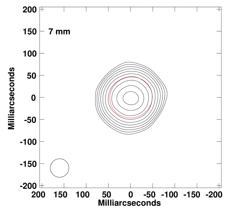
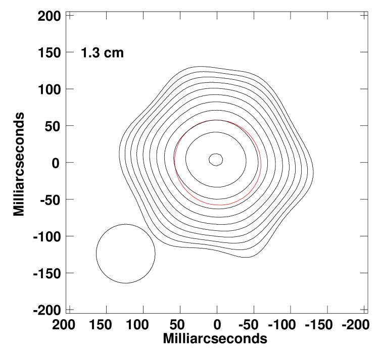
Figure 1.— CLEAN contour maps of Betelgeuse obtained on 2019 August 2 at 7 mm (44 GHz; left) and 1.3 cm (22 GHz; right). Contour levels are ($-$10[absent], 10, 14.1, 20, 28.3, 40, 56.6, 80, 113.1, 160, 200)$\times 29.1\mu$Jy beam^-1 (44 GHz) and ($-$10[absent], 10, 14.1, 20, 28.3, 40, 56.6, 80, 113.1, 160, 226, 319)$\times 15.7\mu$Jy beam^-1 (22 GHz) where the lowest contours are 10$\sigma$. The adopted restoring beam is shown in the lower left of each panel (see Table 2). The red ellipses indicate the best-fitting uniform elliptical disk models (Table 3).

3. Observations

On 2019 August 2 we carried out new continuum observations of Betelgeuse at 44 GHz (Q-band; $\lambda\sim 7$ mm) and 22 GHz (K-band; $\lambda\sim 1.3$ cm) using the VLA in its most extended (A) configuration. Antenna separations ranged from 0.68 km to 36.4 km. At $\lambda$7 mm, this configuration provided angular resolution of $\sim$42 mas, comparable to the size of Betelgeuse’s disk in the near infrared (see Section 2). At $\lambda$1.3 cm the angular resolution was $\sim$80 mas.

The Q-band observations were obtained using the 3-bit observing mode and dual circular polarizations. The WIDAR correlator was configured with four baseband pairs tuned to contiguously cover a frequency window of $\sim$7.9 GHz, centered near 44 GHz. Each baseband pair contained either 15 or 16 subbands, each of which had a bandwidth of 128 MHz and 128 spectral channels. An analogous setup was used for the K-band observations, but with a center frequency of $\sim$22 GHz. To improve $u$-$v$ coverage, observations in the two bands were interleaved during a 4.0 hour session, spanning approximately 14:45–18:45 UTC. Total integration time on Betelgeuse was $\sim$62 min in Q band and $\sim$42 min in K band and the observed elevation of the star ranged from 43 deg to 63 deg. Data were recorded with 2-second time resolution.

The observations were carried out during the late morning and early afternoon local time. Weather conditions ranged from clear to partly cloudy with wind speeds $\leq$4.2 m s^-1. The RMS atmospheric phase fluctuations reported at the VLA site were 6–7 deg during the first half of the observations and 12–17 deg during the second half. Antenna pointing corrections were evaluated hourly using observations of a strong point source at X-band (8 GHz). 3C48 was observed in both K and Q band to allow calibration of the absolute flux density scale (see Section 4). To calibrate the atmospheric phases, fast switching was used between Betelgeuse and two neighboring gain calibrators: J0532+0732 (“cal 1”) and J0552+0313 (“cal 2”), which lie at projected separations of $5^{\circ}\,.58$ and $4^{\circ}\,.22$, respectively, from the star. For Q-band, the adopted observing sequence was: [$t_{\rm cal1},(t_{\rm star},t_{\rm cal2})\times 4,t_{\rm star},t_{\rm cal1}...$], where $t_{\rm cal1}=$ 44 sec, $t_{\rm star}=$46 sec, and $t_{\rm cal2}=$38 sec. For K-band the sequence was: [$t_{\rm cal1},(t_{\rm star},t_{\rm cal2})\times 2,t_{\rm star},t_{\rm cal1}...$], where $t_{\rm cal1}=$ 42 sec, $t_{\rm star}=$ 132 sec, and $t_{\rm cal2}=$ 36 sec.

4. Data Reduction

Data reduction and calibration were performed using the Astronomical Image Processing System (AIPS; Greisen 2003). The original archival science data model files were loaded into AIPS using the Obit software package (Cotton 2008). However, the default calibration (‘CL’) table was regenerated to update the gain and opacity information, and antenna positions were updated to the best available values.

After flagging visibly corrupted data, a requantizer gain correction was applied using the AIPS task TYAPL. Instrumental delays were corrected via fringe fitting to a 1-minute segment of 3C48 data, with separate delay solutions determined for each of the four independent basebands. Bandpass calibration was performed in the standard manner using J0532+0732 as the calibrator; a spectral index of $\alpha\approx$0 was assumed (Healey et al. 2007).

The flux density calibrator 3C48 was known to be undergoing a flare during 2019; therefore special care was taken with the absolute flux density calibration of our data. Clean component models of 3C48 appropriate for the two observing bands were obtained from NRAO via anonymous ftp. The models were derived by R. Perley from observations of 3C48 in the VLA A configuration in 2019 October and were used to set the absolute flux density scale, assuming the standard coefficients of Perley & Butler (2017). We found that the differences in the derived flux density scales based on the 2019 October Perley models compared with the default (non-flaring) models for 3C48 were $\sim$2% in Q band and $\sim$3% in K band, respectively. Thus uncertainty in the absolute flux calibration scale resulting from the flare is expected to be quite small.

As a check that the 2019 October Perley model is suitable for calibrating our measurements, we imaged 3C48 using our new data and found the source structure to be virtually indistinguishable from that seen in the Perley model images, consistent with minimal change in the source at K and Q band frequencies between the date of our observations (2019 August 2) and the date of Perley’s observations (2019 October 24). As a final check on the robustness of our flux density scale, we compared our VLA measurements of the bandpass/complex gain calibrator J052+0732 with a 91.5 GHz measurement from the ALMA obtained on 2019 July 26 with an independent absolute flux density calibrator. Because of the flat spectral index of the source, we expect similar flux densities at 91.5 GHz, 44 GHz, and 22 GHz, and consistent with this, the reported ALMA flux density was 1.22$\pm$0.06 Jy, in good agreement with our VLA measurements (Table 1).

Table 1Calibration Sources

Source	$\alpha$(J2000.0)	$\delta$(J2000.0)	Flux Density (Jy)	$\nu$ (GHz)
3C48a	01 37 41.2994	33 09 35.133	0.6134∗	44.0
…	…	…	1.2194∗	22.0
J0532+0732b	05 32 38.9985	07 32 43.346	1.131$\pm$0.034	44.0
…	…	…	1.172$\pm$0.009	22.0
J0552+0313c	05 52 50.1015	03 13 27.243	0.569$\pm$0.020	44.0
…	…	…	0.734$\pm$0.006	22.0

Note. — Units of right ascension are hours, minutes, and seconds, and units of declination are degrees, arcminutes, and arcseconds. Explanation of columns: (1) source name; (2) & (3) right ascension and declination (J2000.0); (4) derived flux density in Jy at the frequency indicated in column 5; (5) frequency at which the flux density in the fourth column was computed.

Calibration of the frequency-independent portion of the complex gains was performed in the standard manner using the measurements of the gain calibrators J0532+0732 and J0552+0313. Initially, phase-only corrections were solved for using these sources and applied to Betelgeuse using linear interpolation in time. This was followed by similarly computed amplitude and phase corrections. The rms scatter in the phase solutions for the two calibrators was  $<$$\sim$5 deg in Q band and  $<$$\sim$2 deg in K band, respectively, for all antennas.

Following application of the computed gain solutions to Betelgeuse, an additional iteration of phase-only self-calibration was performed for each of the bands using the emission from Betelgeuse itself, with 30 s solution intervals. This step resulted in improvements in the rms noise of of images of 18% and 37%, respectively, for Q and K bands, and the correlated amplitude of the star increased by 52% and 19%, in the two bands, respectively, following the self-calibration.

At this stage, optimized weights for the visibility data were calculated using the AIPS task REWAY. Finally, the data in each band were averaged in frequency to produce 8 spectral channels in each of the 62 subbands.

Images of Betelgeuse were produced from the fully calibrated data using CLEAN deconvolution as implemented in AIPS. Robust weighting with R=0 was adopted, along with a circular restoring beam (see Table 2). Images of the star at the two observing wavelengths are shown in Figure 1. The images appear relatively smooth and symmetric at both wavelengths (but see also Section 5). Note that the apparent six-pointed shape seen in the outer contours of the 1.3 cm image in Figure 1 is an artifact caused by imperfect deconvolution of the VLA’s dirty beam, which has a six-pointed pattern whose first sidelobes overlap with the outskirts of the stellar emission distribution in this band.

Table 2CLEAN Image Properties

Band	$\nu_{\rm GHz}$	$\theta_{\rm a}$	$\theta_{\rm b}$	PA	$\theta_{\rm circ}$	RMS noise
	(GHz)	(mas)	(mas)	(degrees)	(mas)	($\mu$Jy beam-1)
Q	44	43.8	40.7	$+13.7$	42.0	29.0
K	22	87.0	73.8	$+10.2$	80.0	15.9

Note. — CLEAN images were produced using robust (${\cal R}$=0) weighting. $\nu_{\rm GHz}$ is the center frequency in GHz. $\theta_{\rm a}$ and $\theta_{\rm b}$ are the FWHM major and minor axes, respectively, of the dirty beam. The position angle (PA) of the dirty beam was measured east from north. The images presented in Figure 1 were produced using circular restoring beams with the FWHM diameter $\theta_{\rm circ}$ (column 6); these values represent the geometric mean of the dirty beam dimensions in columns 3 & 4.

Table 3Measured Stellar Parameters

Band	$\nu$	$\theta_{\rm maj}$	$\theta_{\rm min}$	PA	$e$	$S_{\nu}$	$D$	$T_{b}$
	(GHz)	(mas)	(mas)	(degrees)		(mJy)	(AU)	(K)
(1)	(2)	(3)	(4)	(5)	(6)	(7)	(8)	(9)
Uniform Elliptical Disk Fits to Visibility Data
Q	43.9	96.9$\pm$2.9 (0.2)	92.6$\pm$2.8 (0.2)	$111.0\pm$5.1 (1.2)	0.04$\pm$0.04	22.34$\pm$2.41 (0.03)	21.1	2270$\pm$260
K	22.0	118.8$\pm$5.9 (0.3)	114.5$\pm$5.7 (0.3)	54.7$\pm$5.2 (1.5)	0.04$\pm$0.07	9.64$\pm$0.97 (0.01)	25.9	2580$\pm$260
Elliptical Gaussian Fits to Image Data
Q	43.9	66.8$\pm$2.1 (0.5)	63.6$\pm$2.0 (0.5)	111.0$\pm$7.8 (6.0)	0.05$\pm$0.04	23.0$\pm$2.5 (0.01)	…	…
K	22.0	79.4$\pm$4.0 (0.6)	73.4$\pm$3.7 (0.6)	67.5$\pm$6.6 (4.3)	0.07$\pm$0.07	9.63$\pm$1.04 (0.01)	…	…

Note. — Quoted uncertainties include formal, systematic, and calibration errors (see Text for details) but not uncertainties in the stellar distance. For measured quantities the value in parentheses indicates the error budget contribution from formal fitting uncertainties. For a uniform elliptical disk, $\theta_{\rm maj}$ and $\theta_{\min}$ are the major and minor axis dimensions, respectively; for a Gaussian fit they represent the the FWHM dimensions of the elliptical Gaussian after deconvolution from the dirty beam. Explanation of columns: (1) observing band; (2) mean observing frequency; (3) FWHM diameter of the major axis in mas; (4) FWHM diameter of the minor axis in mas; (5) PA of the major axis in degrees, measured east from north; (6) ellipticity, defined as $e=(\theta_{\rm maj}-\theta_{\rm min})/(\theta_{\rm maj})$; (7) flux density in mJy; (8) mean size in AU, derived using the geometric mean angular diameter and assuming a distance of 222 pc; (9) brightness temperature in Kelvin, as derived assuming a uniform elliptical disk morphology (see Equation 1).

5. Results

5.1. Measured Stellar Parameters

To characterize the size and flux density of Betelgeuse in our two VLA observing bands we performed fits of a two-dimensional (2D) uniform elliptical disk to the visibility data using the AIPS OMFIT task. As a consistency check, we also fitted elliptical Gaussian models to CLEAN deconvolved images (see Table 2 and Figure 1) using the AIPS JMFIT task. Results are summarized in Table 3. The quoted uncertainties include contributions from the formal fitting uncertainties (Condon 1997), as well as from calibration and systematic errors (see Matthews, Reid, & Menten 2015 for details). The dominant source of uncertainty in the derived flux densities is the absolute calibration uncertainty, assumed to be 10% in both observing bands.

At both observed wavebands the angular diameter measurements are consistent to within uncertainties with previous spatially resolved observations of Betelgeuse at comparable wavelengths (Lim et al. 1998; O’Gorman et al. 2015). As expected for optically thick emission, we measure a larger angular size for the star at the longer of our two observing wavelengths. The mean shape of the radio emitting surface was nearly circular during the epoch of our observations, with an ellipticity of at most a few per cent. The mean angular diameters (taken as the geometric mean of the major and minor axes measured from the visibility data) are 94.7 mas at $\lambda$7 mm and 116.6 mas at $\lambda$1.3 cm, respectively, corresponding to $\sim 2.1$ and $\sim 2.6$ times the near-infrared diameter of the star (see Section 2). For comparison, the angular extent of chromospheric emission traced by the UV “continuum” (centered near $\lambda$2500 Å) is approximately 125$\pm$5 mas, or $\sim 2.8R_{\star}$ in radial units (Gilliland & Dupree 1996), while chromospheric Mg ii emission lines are detected out to projected radii of $\sim$48–135 mas ($\sim$1.1–6$R_{\star}$; Uitenbroek et al. 1998; Dupree et al. 2020).

While the measured angular size of Betelgeuse at both $\lambda$7 mm and $\lambda$1.3 cm is consistent with past observations, the total flux densities in both observing bands are notably lower than previously published values. Among six published $\lambda$1.3 cm measurements between 1996–2004 (Lim et al. 1998; O’Gorman et al. 2015), only one (8.96$\pm$0.24 mJy; obtained in 2002 April) was comparably faint as our current measurement. O’Gorman et al. (2015) found that the 1.3 cm flux density appears to be correlated with the optical ($V$) magnitude, and the 2002 measurement corresponded to a phase when the star was near its minimal optical brightness during its 400-day pulsation cycle ($\phi\approx$0.5). However, at the time of our latest measurements, Betelgeuse was at an intermediate phase ($\phi\approx$0.09). There is no optical photometry available during a window from approximately 100 days preceding our VLA measurements on 2019 August 2 until 10 days after that date, since the star was a daytime object for ground-based observers. Based on an extrapolation of the light curve presented by Dupree et al. (2020), the estimated $V$ magnitude is $\sim$0.65, which is within the typical range for this phase. To our knowledge, no published 1.3 cm measurements are available between 2005–2019, so the more recent behavior of the star at this wavelength is unknown.

At $\lambda$7 mm, the discrepancy between our new measurement and previous results is even more pronounced. Based on four measurements taken between 1996 and 2004, the 7 mm flux density of Betelgeuse remained nearly constant (28.4$\pm 0.5$ mJy, where the error bar indicates the measurement dispersion; Lim et al. 1998; O’Gorman et al. 2015). However, the 7 mm flux density we measure in 2019 August is $\sim$20% (2$\sigma$) lower, even after accounting for calibration uncertainties.

O’Gorman et al. (2015) noted that despite evidence for a systematic dimming of Betelgeuse at radio wavelengths, its spectral index has remained effectively constant over several decades: $\alpha=1.33\pm 0.02$. Based on our current measurements we find $\alpha=1.22\pm 0.22$. Thus to within uncertainties the spectral index remains consistent with previous measurements, although it is poorly constrained since we have only two observing bands.

5.2. Brightness Temperature

Because the radio emission from Betelgeuse is optically thick and our VLA observations are spatially resolved, it is possible to use the angular sizes and flux density measurements from Table 3 to derive a brightness temperature that provides a direct measurement of the mean gas (electron) temperature via the Rayleigh-Jeans expression:

$$T_{B}=2S_{\nu}c^{2}(4.25\times 10^{-28})/(k\nu^{2}\pi\theta_{\rm maj}\theta_{\rm min})$$ (1)

where $S_{\nu}$ is in mJy, $\theta_{\rm maj}$ and $\theta_{\rm min}$ are the dimensions of the best-fitting disk model in units of mas (see Table 3), $c$ is the speed of light in cm s^-1, $k$ is the Boltzmann constant in cgs units, and $\nu$ is the mean observing frequency in GHz. At $\lambda$7 mm we find $T_{B}=2270\pm 260$ K (corresponding to $r\sim 2.1R_{\star}$) and at $\lambda$1.3 cm $T_{B}=2580\pm$260 K (corresponding to $r\sim 2.6R_{\star}$). The derived brightness temperature at $\lambda$1.3 cm is at the low end of previously observed values at this wavelength (O’Gorman et al. 2015) and is markedly cooler than the value of $\sim$3300 K reported at this wavelength by Lim et al. (1998). At $\lambda$7 mm, the $T_{B}$ value measured in 2019 August is the lowest ever reported at this wavelength. In comparison, Lim et al. (1998), measured a brightness temperature at $\lambda$7 mm of 3450$\pm$850 K (based on data from 1996), comparable to the mean photospheric temperature of Betelgeuse, while O’Gorman et al. (2015) reported values of 3040$\pm$80 K, 2760$\pm$200 K, 2940$\pm$140 K for data obtained in 2000, 2003, and 2004, respectively. The semi-empirical model of Harper et al. (2001) (which was originally based on the Lim et al. measurements) predicts a characteristic temperature at $r\sim 2.1R_{\star}$ of $\sim$1500 K hotter than seen in our current data (see Figure 4, discussed below). Indeed, the temperature that we measure based on our new 7 mm data is only slightly warmer than that within the molecular layer known as the “MOLsphere”, which extends from $r\sim$1.3–1.5$R_{\star}$ and has an estimated temperature of $\sim$1500-2000 K (Tsuji 2000, 2006). We discuss the implications of these temperature measurements further in Section 5.4.

5.3. Deviations from a Uniform Disk

5.3.1 Evidence for a Multi-component Brightness Profile

The uniform elliptical disk fits we have employed above are useful for providing a characterization of the mean properties of the star (angular size, temperature). However, the high signal-to-noise ratio of our current data—roughly an order of magnitude higher than previous radio images of Betelgeuse at comparable wavelengths—allows us to see clear evidence of deviation from this simple model.

In Figure 2 we plot the azimuthally averaged visibility data (real and imaginary parts) as a function of $u$-$v$ distance for our two observing bands, with the best-fitting uniform elliptical disk models overplotted. In each band we see that the uniform elliptical disk model under-represents the observed flux on the smallest observed angular scales (longest baselines) while systematically slightly over-predicting the flux density on scales sampled by intermediate baselines ($\sim$0.5–1.5M$\lambda$).

If we subtract the best-fitting uniform elliptical disk model from the visibility data and Fourier transform the residuals to make an image, an outer “ring” of positive residuals is visible in both the 7 mm and 1.3 cm data, surrounding a negative trough and a positive central peak coincident with the star’s center (Figure 3, top row). The peak residuals are $~{}\hbox to0.0pt{$<$\hss}{\lower 4.30554pt\hbox{$\sim$}}12\sigma$ in the 7 mm image and $~{}\hbox to0.0pt{$<$\hss}{\lower 4.30554pt\hbox{$\sim$}}6.5\sigma$ in the 1.3 cm image.

The fits to both the 7 mm and 1.3 cm data are improved by the introduction of a second component to the model. Results of a two-component elliptical disk model (Model 1) and an elliptical disk+ring model (Model 2) are shown on the upper panels of Figure 2 as dashed lines and dotted lines, respectively. The model parameters are summarized in Table 4. Both of these models result in a significant reduction of the residuals in the image domain (Figure 3, middle and lower panels), although for the 7 mm data both models still underpredict the visibility amplitude at large $u$-$v$ distances ($<5$M$\lambda$; Figure 2), with the discrepancy being larger for the disk+ring model. At $\lambda$1.3 cm the fit quality for Models 1 and 2 is similar. We stress that neither of these two-component models is unique, nor do they have an obvious underlying physical underpinning. However, it is noteworthy that because the two components are concentric, the presence of a large convective cell (cf. Lim et al. 1998) or other transient surface feature cannot readily account for presence of the second component.

It is unclear whether this multi-component brightness profile is unique to our 2019 observations, as previous spatially resolved observations of Betelgeuse at comparable wavelengths were obtained prior to the VLA’s sensitivity upgrade (Perley et al. 2011), making the unambiguous identification of similar features more difficult. However, hints of deviation from a simple uniform elliptical disk model are seen in fits to earlier data (cf. Figure 2 of O’Gorman et al. 2015). In addition, O’Gorman et al. (2017) also found a multi-component model necessary to fit their 2015 ALMA 338 GHz observations of Betelgeuse, and a similar behavior was seen in 7 mm observations of the nearby carbon star IRC+10216 (Matthews et al. 2018). In general the identification of such trends is important for constraining models of the electron temperature as a function of radius in red supergiant atmospheres (see, e.g., Figure 3 of Harper et al. 2001) and underscores the unique power of high-sensitivity, spatially resolved radio observations.

5.3.2 No Evidence for Giant Convective Cells

Based on their 7 mm VLA observations, Lim et al. (1998) reported a significant brightness asymmetry that they interpreted as possible evidence of a large convective cell in the atmosphere of Betelgeuse. They noted that such features may be linked with upwellings of cool photospheric gas and may play a role in the mass-loss process of red supergiants. Indeed, it has been suggested that the recent Great Dimming may have been caused by a mass-loss event tied to the surfacing of a giant convective cell (Montargès et al. 2021). However, our VLA measurements from 2019 August do not reveal any direct evidence for the presence of such features; we see neither morphological evidence of giant “cells” nor signatures of enhanced radio emission. As discussed in Sections 5.1 and 5.3.1, the star appears largely symmetric and uniform, although the imaginary parts of the visibility data (Figure 2, right panels) do show some low-level fluctuations that may reflect small brightness variations across the star. One possible explanation is that any observable effects of a photospheric convective cell within the regions sampled by our observations had already disappeared after “surfacing” between 2019 January–April.

5.4. Discussion

As shown in Figure 4, the brightness temperature values that we derive from our 2019 August 2 observations of Betelgeuse at $\lambda$7 mm and $\lambda$1.3 cm lie significantly below the predictions of the semi-empirical model of Harper et al. (2001). The compendium of Betelgeuse radio measurements presented by O’Gorman et al. (2015) shows that within the period from 1996–2004, the 1.3 cm flux density appears to have systematically decreased by $\sim$20% compared with the earlier measurements of Newell & Hjellming (1982) (which spanned 1972–1981) and Drake et al. (1992) (which spanned 1986–1990). The physical mechanism that might explain such systematic dimming is unclear, although it may be linked with long-term changes in the underlying dynamics of the star (e.g., George et al. 2020). To our knowledge, no radio light curve data for Betelgeuse are available between 2005 and mid-2019. Therefore we are unable to determine conclusively whether our present measurements point to a continued, systematic dimming trend of Betelgeuse at cm wavelengths, reflect normal temporal variations—or alternatively, may be linked with atmospheric changes leading up to the UV outburst detected by Dupree et al. (2020) and/or the subsequent Great Dimming. Here we briefly discuss this latter possibility.

As discussed in the previous section, our VLA observations of Betelgeuse on 2019 August 2 do not appear to show any unambiguous morphological signatures of an ongoing atmospheric disturbance in early 2019 August, roughly one month prior to the onset of the outflow event documented by Dupree et al. (2020). Despite this, our radio measurements are consistent with the possibility that the atmosphere of Betelgeuse may have undergone marked physical changes near the time of the outburst. Indeed, the anomalously low brightness temperatures that we measure between $r\sim 2$–$3R{\star}$, as well as the apparent temperature inversion within this radial range, point to significant changes density and/or ionization fraction within this region compared with previous epochs.

As briefly described in Section 1, the tomographic analysis of Kravchenko et al. (2021) revealed evidence for the the occurrence of successive shock waves through the photosphere of Betelgeuse in 2018 February and 2019 January, with the initial shock serving to amplify the second one. Subsequently, spatially resolved spectroscopic measurements in the UV by Dupree et al. (2020) revealed that a shock or pressure wave passed through the southwestern portion of Betelgeuse’s chromosphere between 2019 September and November. (The exact time of the onset of this latter event is not precisely known, but evidence for a disturbance was not seen during the previous epoch of UV observations in 2019 March). Concurrent measurements of the C ii lines at 2325 and 2328Å also point to increases in the temperature and electron density in the southern hemisphere of Betelgeuse. Importantly, the UV measurements of Betelgeuse’s chromosphere from Dupree et al. (including the Mg ii lines and continuum) probe approximately the same range of projected radii as our current VLA observations ($\sim$2–3$R_{\star}$). These events are therefore also expected to impact the radio continuum emission near the same time period.

As discussed by Reid & Menten (1997), the propagation of pulsationally-induced shocks through the extended atmosphere of a red giant ($r~{}\hbox to0.0pt{$>$\hss}{\lower 4.30554pt\hbox{$\sim$}}2R_{\star}$) may produce temperature and density variations as a function of radius that may in turn lead to variations in the observed radio emission. In a simple version of this model, the temperature as a function of radius, $T(r_{0})$, predicted by a hydrostatic model of the extended atmosphere becomes instead:

$$T(r_{0})=\left<T(r_{0})\right>+\Delta T_{s}{\rm cos}\left(\phi_{p}+\phi_{s}\right)$$ (2)

where $\Delta T_{s}$ is the amplitude of the temperature contrast between the pre- and post-shock gas, $\phi_{p}$ is the stellar phase, and $\phi_{s}$ is the phase of the propagating disturbance. Following Reid & Menten, if one assumes a shock propagation speed $V_{s}$ and a pulsation period $P$, then $\phi_{s}$ can be defined as

$$\phi_{s}=2\pi\frac{r-R_{\star}}{V_{s}P}$$ (3)

Figure 4 (dotted line) shows an example of the effect of this toy model on the radial temperature profile. We based the shape of the input temperature profile on the semi-empirical model atmosphere of Harper et al. (2001), but have applied a temperature offset of $-1000~{}K$ (thin solid line). Here we have adopted $P$=400 days (comparable to Betelgeuse’s “short” pulsation period; see Section 1), $V_{s}$=7.0 km s^-1, and $\Delta T_{s}$=250 K. We show the results for a single value of the shock excitation phase, $\phi_{p}$=0.09. The exact combination of parameters is somewhat arbitrary. Nonetheless, this toy model qualitatively illustrates that a disturbance of this kind may be able to account for: (i) a (temporary) distortion of the temperature profile, including a possible temperature reversal between the radial regions sampled by the 7 mm and 1.3 cm radio emission, respectively; (ii) corresponding modulations in the radio flux densities; and (iii) temperature and electron density fluctuations across the chromospheric regions probed by the HST UV measurements of Dupree et al. 2020). One important test of this scenario will be follow-up observations of Betelgeuse at radio wavelengths to assess whether the star has since returned to its historical flux density levels.

Table 4Multi-Component Model Fit Parameters

Comp.	E offset (mas)	N offset (mas)	$\theta_{a}$ (mas)	$\theta_{b}$ (mas)	PA (deg)	$S_{\nu}$ (mJy)
Model 1 ($\lambda$=7 mm)
Uniform Elliptical Disk	0.25$\pm$0.22	0.09$\pm$0.21	125.6$\pm$1.6	116.5$\pm$1.3	$-33.6\pm 1.7$	12.5$\pm$0.5
Uniform Elliptical Disk	$-$0.24$\pm$0.16	0.05$\pm$0.13	78.3$\pm$0.1	69.1$\pm$0.1	$-93.7\pm 1.2$	10.6$\pm 0.6$
Model 2 ($\lambda$=7 mm)
Uniform Elliptical Disk	$-$0.07$\pm$0.08	0.01$\pm$0.07	81.2$\pm$0.8	76.1$\pm$0.8	$95.6\pm 1.1$	17.2$\pm 0.6$
Elliptical Ring	0.29$\pm$0.26	$-$0.01$\pm$0.03	110.5$\pm$1.4	101.6$\pm$1.1	147.6$\pm 1.7$	5.9$\pm$0.2
Model 1 ($\lambda$=1.3 cm)
Uniform Elliptical Disk	0.26$\pm$0.12	0.70$\pm$0.15	98.8$\pm$1.9	91.6$\pm$2.4	174.7$\pm$2.0	6.5$\pm$0.3
Uniform Elliptical Disk	$-1.20\pm 0.49$	$-3.6\pm 0.63$	183.3$\pm$5.3	166.8$\pm$4.3	120.0$\pm$2.4	3.3$\pm$0.3
Model 2 ($\lambda$=1.3 cm)
Uniform Elliptical Disk	0.03$\pm$0.08	0.06$\pm$0.09	98.9$\pm$2.0	92.9$\pm$2.2	77.5$\pm$1.7	7.7$\pm$0.2
Elliptical Ring	$-1.19\pm 0.48$	$-3.7\pm 0.65$	151.1$\pm$4.1	137.3$\pm$3.3	26.9$\pm$2.2	2.1$\pm$0.2

Note. — Quoted error bars include only formal fitting uncertainties. The models are shown overplotted on the visibility data in Figure 2.

6. Summary

We have presented spatially resolved VLA imaging observations of the radio emission from Betelgeuse at wavelengths of 7 mm and 1.3 cm. The data were obtained on 2019 August 2, just prior to the onset of the Great Dimming of the star in late 2019 and early 2020. At both observed wavelengths the star appears spherically symmetric with no evidence of large-scale brightness non-uniformities. However, the brightness profile in both bands is found to be more complex than a simple uniform elliptical disk.

We find the 7 mm flux density of Betelgeuse to be $\sim$20% lower than previously published measurements during the past 25 years. The mean brightness temperature derived from the 7 mm observations, which probes gas at a mean projected radius of $r\sim 2.1R_{\star}$, is also significantly lower compared with previous measurements at comparable radii and lies  $>$$\sim$1200 K below the prediction of published semi-empirical models of Betelgeuse’s extended atmosphere. The brightness temperature derived from the 1.3 cm data (which probes material at $r\sim 2.6R_{\star}$) is also lower than expected based on trends in historical measurements. Our new data therefore suggest recent changes in the density and/or temperature structure of the atmosphere between $\sim 2$–$3R_{\star}$. One possible explanation is the recent passage of a large-amplitude shock or pressure wave through the outer atmosphere. This picture can also account for atmospheric disturbances revealed by UV imaging spectroscopy by Dupree et al. (2020) during the two months following the VLA observations. Such an event may be linked to a large-scale mass ejection from the star that has been postulated as an explanation for the steep decline in optical magnitude associated with the Great Dimming.

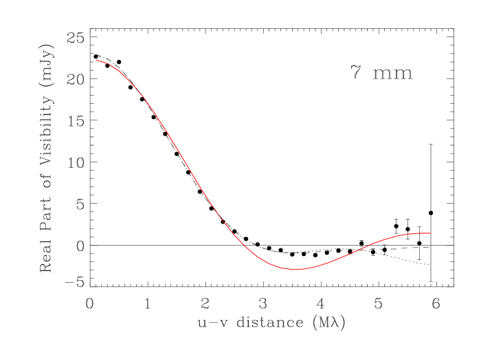
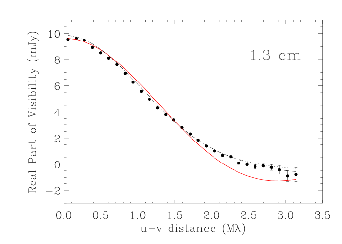
Figure 2.— Real (top) and imaginary (bottom) parts of the visibility amplitude vs. baseline length for observations of Betelgeuse at $\lambda$7 mm (left) and $\lambda$1.3 cm (right). On the upper panels the solid red lines indicate the best-fitting uniform elliptical disk models from Table 3. The two-component models from Table 4 are overplotted as black dashed lines (Model 1) and dotted lines (Model 2).

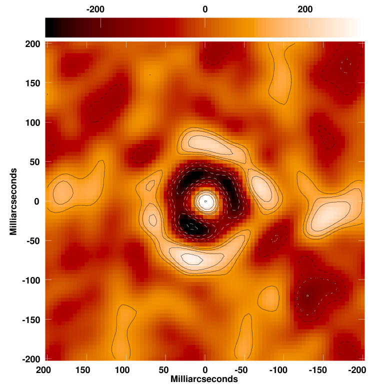
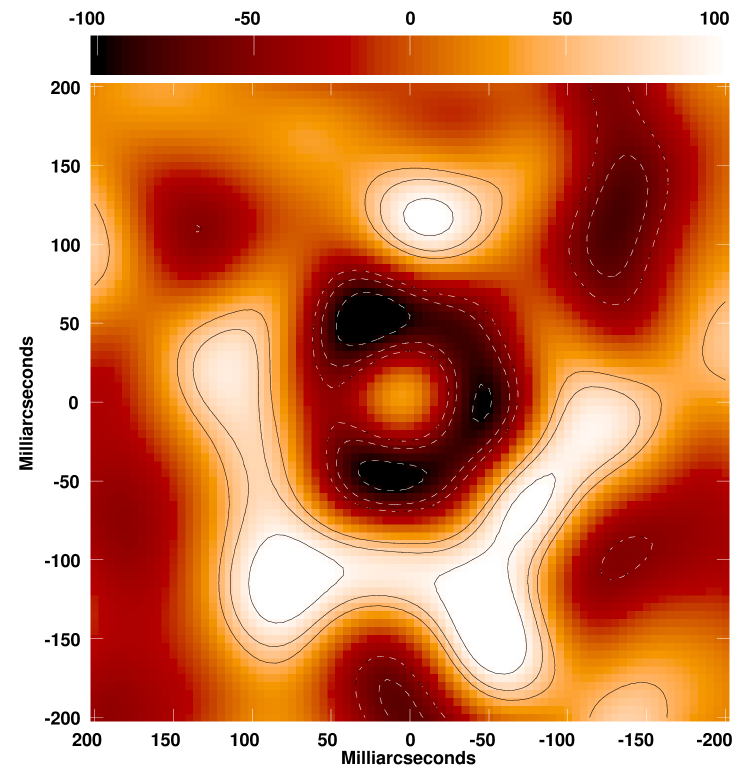
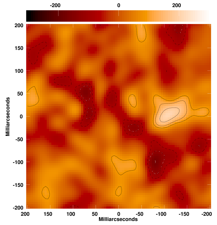
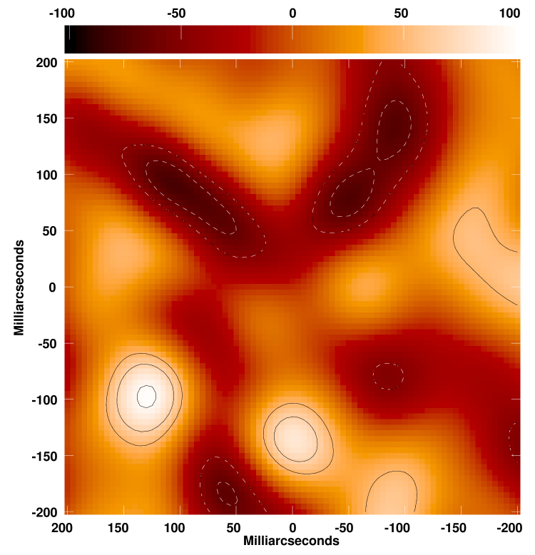
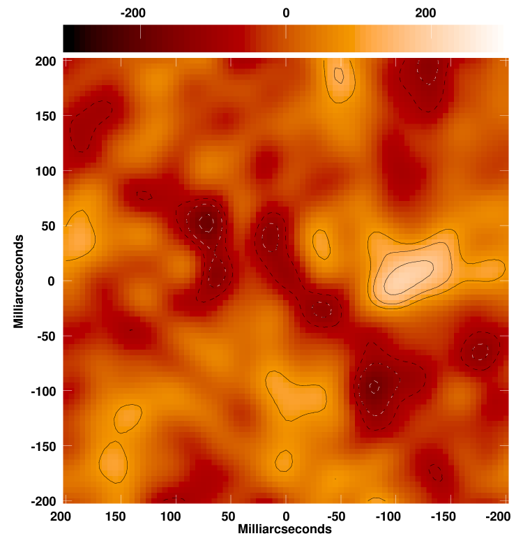
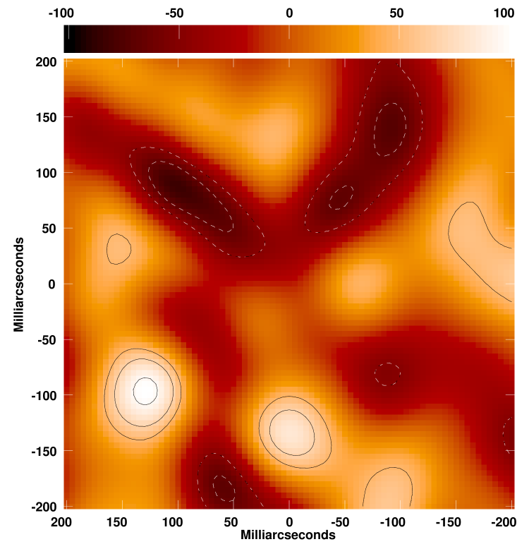
Figure 3.— Residual maps obtained by imaging the $\lambda$7 mm data (left) and $\lambda$1.3 cm data (right) from 2019 August 2, after subtraction of model fits from the visibilities. Top row: residuals from best-fitting uniform elliptical disk model (see Table 3); Middle row: residuals from a model comprising two uniform elliptical disk components (Model 1, Table 4); Bottom row: residuals from a model comprising a uniform elliptal disk and elliptical ring (Model 2, Table 4). Intensity units are $\mu$Jy beam^-1. Contours are [$-12,-8.5,-6,-4.2,-3,3,...,12]\times\sigma_{\nu}$ where $\sigma_{\nu}$ is the 1$\sigma$ RMS noise in the respective band (Table 2). Negative contours are shown as dashed lines.

Figure 4.— Schematic illustration of the effects of a propagating shock wave on the radial temperature profile of the extended atmosphere of Betelgeuse. The assumed shape of the underlying temperature profile is based on the semi-empirical model of Harper et al. (2001). The thick solid line shows the temperature predicted by the original model; the thin solid line shows the same model with a temperature offset of $-$1000 K. The dotted line shows the temperature perturbations to the latter model resulting from a periodic disturbance with $P$=400 days, amplitude $\Delta T_{s}=\pm 250$ K, and propagation speed $V_{s}=$7.0 km s^-1 (see text for details). The triangle symbols indicate the brightness temperatures derived from the 2019 August 2 VLA measurements.

References

- (1) Altenhoff, W. J., Oster, L., & Wendker, H. J. 1979, A&A, 73, L21
- (2) Brandt, J. C., Heap, S. R., Beaver, E. A., et al. 1995, AJ, 109, 2706
- (3) Calderwood, T. 2021, S&T, 141, 14
- (4) Condon, J. J. 1997, PASP, 109, 166
- (5) Cotton, D. V., Bailey, J., De Horta, A., Norris, B. R. M., & Lomax, J. R. 2020, RMAAS, 4, 39
- (6) Cotton, W. D. 2008, PASP, 120, 439
- (7) Dharmawardena, T. E., Mairs, S., Scicluna, R., et al. 2020, ApJL, 897, L9
- (8) Drake, S. A., Bookbinder, J. A., Florkowski, D. R., Linsky, J. L., Simon, T., & Stencel, R. E. 1992, Cool Stars, Stellar Systems, and the Sun, edited by M. S. Giampapa and J. A. Bookbinder, ASP Conf. Series, 26, 455
- (9) Dupree, A. 2018, HST Proposal #15641
- (10) Dupree, A. K., Strassmeier, K. G., Matthews, L. D., et al. 2020, ApJ, 899, 68
- (11) Dyck, H. M., Benson, J. A., Ridgway, S. T., & Dixon, D. J. 1992, AJ, 104, 1982
- (12) George, S. V., Kachhara, S., Misra, R., & Ambika, G. 2020, A&A, 640, L21
- (13) Gilliland, R. L. & Dupree, A. K. 1996, ApJ, 463, L29
- (14) Greisen, E. W. 2003, Information Handling in Astronomy—Historical Vistas, ed. A. Heck (Dordrecht: Kluwer), 109
- (15) Guinan, E., Wasatonic, R., Calderwood, T., & Carona, D. 2020, ATel, 13512, 1
- (16) Harper, G. M., Brown, A., Guinan, E. F., O’Gorman, E., Richards, A. M. S., Kervella, P., & Decin, L. 2017, AJ, 154, 11
- (17) Harper, G. M., Brown, A., & Lim, J. 2001, ApJ, 551, 1073
- (18) Harper, G. M., Guinan, E. F., Wasatonic, R., & Ryde, H. 2020, ApJ, 905, 34
- (19) Hartmann, L. & Avrett, E. H. 1984, ApJ, 284, 238
- (20) Healey, S. E., Romani, R. W., Taylor, G. B., Sadler, E. M., Ricci, R., Murphy, T., Ulvestad, J. S.. & Winn, J. N. 2007, ApJS, 171, 61
- (21) Kellermann, K. I. & Pauliny-Toth, I. I. K. 1966, ApJ, 145, 953
- (22) Kiss, L. L., Szabó, G. M., & Bedding, T. R. 2006, MNRAS, 372, 1721
- (23) Kravchenko, K., Jorissen, A., Van Eck, S., Merle, T., Chiavassa, A., Paladini, C., Freytag, B., Plez, B., Montargès, M., & Van Winckel, H. 2021, A&A, 650, L17
- (24) Levesque, E. M. & Massey, P. 2020, ApJL, 891, L37
- (25) Lim, J., Carilli, C. L., White, S. M., Beasley, A. J., & Marson, R. G. 1998, Nature, 392, 575
- (26) Matthews, L. D., Reid, M. J., & Menten, K. M. 2015, ApJ, 808, 36
- (27) Matthews, L. D., Reid, M. J., Menten, K. M., & Akiyama, K. 2018, AJ, 156, 15
- (28) Montargès, M., Cannon, E., Lagadec, E., et al. 2021, Nature, 594, 365
- (29) Newell, R. T. & Hjellming, R. M. 1982, ApJ, 263, L85
- (30) O’Gorman, E., Harper, G. M., Brown, A., Guinan, E. F., Richards, A. M. S., Vlemmings, W., & Wasatonic, R. 2015, A&A, 580, A101
- (31) O’Gorman, E., Harper, G. M., Ohnaka, K., et al. 2020, A&A, 638, A65
- (32) O’Gorman, E., Kervella, P., Harper, G. M., Richards, A. M. S., Decin, L., Montargès, M., & McDonald, I. 2017, A&A, 602, L10
- (33) Perley, R. A. & Butler, B. J. 2017, ApJS, 230, 7
- (34) Perley, R. A., Chandler, C. J., Butler, B. J., & Wrobel, J. M. 2011, ApJ, 739, 1
- (35) Reid, M. J. & Menten, K. M. 1997, ApJ, 476, 327
- (36) Seaquist, R. R. 1967, ApJL, 148, L23
- (37) Skinner, C. J., Dougherty, S. M., Meixner, M., Bode, M. F., Davies, R. J., Drake, S. A., Arens, J. F., & Jernigan, J. G. 1997, MNRAS, 288, 295
- (38) Tsuji, T. 2000, ApJ, 538, 801
- (39) Tsuji, T. 2006, ApJ, 645, 1448
- (40) Uitenbroek, H., Dupree, A. K., & Gilliland, R. L. 1998, ApJ, 116, 2501
- (41) Začs, L. & Pukītis, K. 2021, RNAAS, 5, 8
- (42)