Characteristics of Kepler Eclipsing Binaries Displaying a Significant O’Connell Effect

Abstract

The O’Connell effect – the presence of unequal maxima in eclipsing binaries – remains an unsolved riddle in the study of close binary systems. The Kepler space telescope produced high precision photometry of nearly 3,000 eclipsing binary systems, providing a unique opportunity to study the O’Connell effect in a large sample and in greater detail than in previous studies. We have characterized the observational properties – including temperature, luminosity, and eclipse depth – of a set of 212 systems (7.3% of Kepler eclipsing binaries) that display a maxima flux difference of at least 1%, representing the largest sample of O’Connell effect systems yet studied. We explored how these characteristics correlate with each other to help understand the O’Connell effect’s underlying causes. We also describe some system classes with peculiar light curve features aside from the O’Connell effect ($\sim$24% of our sample), including temporal variation and asymmetric minima. We found that the O’Connell effect size’s correlations with period and temperature are inconsistent with Kouzuma’s starspot study. Up to 20% of systems display the parabolic eclipse timing variation signal expected for binaries undergoing mass transfer. Most systems displaying the O’Connell effect have the brighter maximum following the primary eclipse, suggesting a fundamental link between which maximum is brighter and the O’Connell effect’s physical causes. Most importantly, we find that the O’Connell effect occurs exclusively in systems where the components are close enough to significantly affect each other, suggesting that the interaction between the components is ultimately responsible for causing the O’Connell effect.

1 Introduction

The O’Connell effect (O’Connell, 1951; Milone, 1968) is a poorly understood asymmetry seen in some eclipsing binaries where the maxima between eclipses are not equal in brightness (see Figure 1). At the quadrature phases ($\phi=0.25,~{}0.75$ for circular orbits), we see the stars side-by-side, so a difference in brightness implies that one hemisphere of a component emits a different amount of radiation than the other hemisphere. Roberts (1906) first discussed the O’Connell effect, where he attributed it to stars in an eccentric orbit becoming tidally distorted near periapsis. His theory did not explain the presence of the O’Connell effect in systems with circular orbits, however, and is no longer considered a likely cause of the O’Connell effect in most systems. Wilsey & Beaky (2009) outlines a few possible explanations for the O’Connell effect: chromospheric spots on one or both components, a hotspot caused by mass transfer, or circumbinary material impacting the stars as they orbit (Liu & Yang, 2003). Wilsey & Beaky (2009) notes that none of these explains the O’Connell effect in all cases, however, and Papageorgiou et al. (2014) states that “the O’Connell effect is still one of the most perplexing challenges in binary studies.”

1.1 Background

O’Connell (1951, hereafter O51) found strong correlations between the O’Connell effect size (OES, also commonly known as $\Delta m$) and the following parameters: the difference in OES at different wavelengths, the ellipticity of the component stars, the ratio of stellar radii, and the ratio of stellar densities. Most notably, he found that the OES becomes larger at shorter wavelengths as the OES increases, which is to say OES_blue – OES_red increases as OES increases. O51 restricted his study to systems with a constant OES and excluded W Ursae Majoris systems.

Davidge & Milone (1984, hereafter D84) built upon the work of O51 by introducing more systems displaying the O’Connell effect and using a second, non-parametric form of analysis less prone to outliers in addition to the parametric analysis used by O51. Like O51, D84 restricted their sample to systems with a constant OES and excluded overcontact systems. The higher precision photometry available to D84 meant that many systems included in O51 were found to have a variable OES and so were excluded. D84 found essentially the same strong correlations as O51. The correlation between the OES and the size at different wavelengths was the strongest correlation in O51 and D84. However, D84 found that the OES becomes larger at longer wavelengths as the OES increases, the opposite of O51’s correlation. They attributed this discrepancy to the sample selection difference between O51 and D84, as there are only six systems in common between the two studies. Note that both O51 and D84 used ground-based data taken in the era before CCDs.

Figure 1: Averaged light curve of KIC 5282464 showing the O’Connell effect. The maximum following the primary eclipse (indicated with the upper dashed line) is noticeably brighter than the maximum preceding it (indicated by the lower dashed line).

Wilsey & Beaky (2009, hereafter W09) is the most recent major work on the O’Connell effect. W09 examines the current theoretical models used to explain the O’Connell effect: starspots, gas stream impacts, circumstellar material, and asymmetric circumfluence due to Coriolis forces. They state that starspots are the most commonly used explanation for the O’Connell effect. These spot models can be used to explain both chromospheric starspots like those found on our Sun and starspots arising from the impact of a matter stream. However, W09 states that the spots need to be unrealistically large to explain the observed O’Connell effect in many systems, and Maceroni & van’t Veer (1993) states that the photometric light curves used to build these models are often insufficient to justify the existence of starspots. Furthermore, starspots introduce four new parameters per spot to the parameter space: spot latitude, longitude, radius, and temperature factor. These additional parameters increase the uniqueness problem (Kallrath & Milone, 2009), making finding the parameter space’s global minimum (and thus the best model of the system) nearly impossible. Next, W09 discusses how a hotspot created by a matter stream can create a maximum difference if it is offset from the central axis connecting the centers of both stars. They also identify two candidate systems where this matter stream hypothesis has explained the O’Connell effect: V361 Lyrae and GR Tauri. Finally, W09 discusses two papers (Liu & Yang 2003 and Zhou & Leung 1990) that propose models for the O’Connell effect. Liu & Yang (2003) proposed that the impact of material surrounding both stars heats the leading hemispheres, causing a difference in brightness and temperature. However, W09 notes that their model’s assumptions are unrealistic. Zhou & Leung (1990) proposed that the deflection of circulating material by Coriolis forces can explain the O’Connell effect in overcontact systems.

Recent surveys such as the Kepler (Borucki et al., 2010) and Transiting Exoplanet Survey Satellite (TESS; Ricker et al., 2014) missions and future surveys such as the Legacy Survey of Space and Time (LSST; Ivezić et al., 2019) conducted by the Vera C. Rubin Observatory provide an enormous amount of data on the variable universe. These surveys uncover and provide complete samples of sources that display poorly understood phenomena (including the O’Connell effect), allowing us to completely characterize these systems for the first time. The first step to understanding these phenomena is determining the characteristics of sources exhibiting them. This characterization allows us to anticipate which newly observed sources might show them and provides clues to the physical processes underlying the phenomenon in question.

1.2 Our Study

Our project aims to characterize the observational properties (including period, color, OES, and eclipse depth) of systems displaying a significant O’Connell effect, which serves as a prelude to understanding the O’Connell effect’s physical causes. We have selected 258 eclipsing binaries observed by Kepler, of which 212 constitute a core sample showing an average $|$OES$|$ larger than 1% of their normalized flux. Our core sample represents the largest sample of O’Connell effect binaries studied to date. This paper describes our characterization of the core sample. In addition to this characterization, we determined how the characteristics correlate with each other. These correlations provide important insights into the processes underlying the O’Connell effect. This paper also details our use of two statistical measures introduced by McCartney (1999) and refined by W09. Our project serves as a continuation of the studies presented in O51 and D84 using modern observational techniques like space-based CCD photometry. However, our lack of bulk physical characteristics (mass, density, surface gravity, etc.) due to lacking radial velocity data forces us to probe a different parameter space than those works.

Our project seeks to answer questions about the O’Connell effect using a sample selected in a consistent and unbiased manner. We primarily see the O’Connell effect in short-period eclipsing binaries, where the stars are close enough to interact with each other. Is this a selection bias, or is there a genuine link between binary interaction and the O’Connell effect? O51 found that the brighter maximum almost uniformly followed the primary eclipse rather than preceding it. D84, by contrast, found a more even distribution of maxima preference, with about 60% of their sample having the brighter maximum follow the primary eclipse. Which result better describes the maxima distribution of the underlying population? Do the characteristics of these systems correlate in the manner Kouzuma (2019) suggests spotted stars should? Or do we instead see the eclipse timing variations characteristic of mass transfer in a majority of systems? Is the OES the best way to characterize the O’Connell effect, or are the O’Connell Effect Ratio and Light Curve Asymmetry statistical measures introduced by McCartney (1999) better? Finally, how common is the O’Connell effect?

We now define the light curve classifications (Algol-, $\beta$ Lyrae-, and W Ursae Majoris-type systems) and morphological classifications (detached, semi-detached, and overcontact) we will adopt in this paper. Algol-type systems have sharp, well-defined eclipses and minimal out-of-eclipse variations, $\beta$ Lyrae-type systems have continuously variable light curves and minima of significantly unequal depth, and W Ursae Majoris-type systems have continuously variable light curves and minima of equal or nearly equal depth. We quantify our light curve classification in Section 3.3. Our light curve classification does not consider the binary components’ spectral type or evolutionary state (e.g. we would classify V382 Cygni as W Ursae Majoris-type rather than $\beta$ Lyrae-type as Landolt 1975 did). Meanwhile, detached systems have neither star filling their Roche lobe, semi-detached systems have one star (either the primary or secondary) exactly filling their Roche lobe, and overcontact systems have both stars overflowing their Roche lobes. We define the primary star as the component eclipsed at the deeper minimum without regard to the component masses.

Section 2 describes how we determined our sample and the biases that are inherent to it. Section 3 discusses our methodology in analyzing the Kepler data. Section 4 gives the characteristics of our core sample, including their light curve properties, information obtained from other sources, and properties derived from available data. Section 4 also describes four system classes with peculiar features in their light curves aside from the O’Connell effect, including temporal variation of their light curves and asymmetric minima. Section 5 discusses the observed trends found in our study and the implications of these trends. Finally, Section 6 summarizes our major results and details future work on this project.

2 Target Selection

We drew our sample from the Kepler Eclipsing Binary Catalog (KEBC), a compilation of eclipsing binary systems observed by the Kepler space telescope. We defined a single criterion to define our sample: $|$OES$|\geq 0.01$, where OES is in units of normalized flux and $|$OES$|$ is the absolute value of the OES that folds the negative OES values over the positive ones. We created a code to determine the OES, which we used to select a core sample of 212 system based on their long-cadence Kepler data.

2.1 Kepler Space Telescope

The Kepler space telescope was launched in 2009 with the purpose of observing transiting planets. The spacecraft imaged over 150,000 objects every thirty minutes for four years, observing numerous variable stars in the process. Kepler’s photometry is accurate within 29 parts per million (ppm) for a star with an apparent magnitude of 12 and 80.7 ppm at an apparent magnitude of 14.5 (Gilliland et al., 2011). For comparison, Tregloan-Reed & Southworth (2013) cites a precision of 258 ppm (of a V = 11.45 star using the 4-meter Mayall telescope; Gilliland et al., 1993) as the most precise ground-based observations known. Therefore, it is clear that Kepler’s photometry is much more precise than ground-based data, even for fainter stars, making features such as kinks or subtle changes over time more apparent. As a result of this precision, we are more confident that any peculiar features observed in a light curve are real structures rather than a result of statistical noise. Some targets have short-cadence data (sampling every minute) in addition to the long-cadence data (sampling every 30 minutes) that all targets have, allowing us to study short-timescale variations in these systems. However, our analysis in this paper is based exclusively on the long-cadence data.

Kepler observed most systems nearly continuously for over three years, providing an opportunity to see how each system changes over that time. Such changes can be attributed to various factors, including starspot evolution, accretion disk instabilities, or a change in temperature due to thermal equilibration. The long observation span and high precision also maximizes our sensitivity to transient effects like flares, allowing us to characterize the prevalence of these events in our sample. Additionally, variations in the eclipse timing can indicate the presence of a third body in the system or an actual change in the period due to mass transfer. Finally, observing targets for such a long, continuous time minimizes the risk of artifacts due to poor sampling or transient effects such as flares. The effects of such artifacts are unpredictable, with one such effect being an oscillatory signal introduced in systems with a period that is a near-integer multiple of the Kepler cadence.

Using Kepler as a basis for our study introduces the same biases inherent to the Kepler mission. The observed targets were drawn from the Kepler Input Catalog (KIC; Brown et al., 2011), which estimated each star’s spectral type and luminosity class based on photometrically determined colors. Batalha et al. (2010) describes the Kepler target prioritization and statistics for the operational target list. They assigned the highest priority to systems with a Kepler magnitude $K_{p}<14$, and where an Earth-sized planet in the habitable zone would produce at least three transits in the 3.5-year mission with a signal-to-noise ratio greater than $7.1\sigma$. They chose the first condition to facilitate follow-up high-precision spectroscopy to confirm planet detections. The second condition, meanwhile, excluded most O- and B-type stars. As a result of this prioritization, there are more G- and F-type stars than K- or M-type stars among Kepler targets, and Kepler only observed $\sim$3,000 M-type stars and fewer than 200 O- and B-type stars. The Kepler target list also has a bias against giants and subgiants because planetary transits are harder to detect due to the smaller ratio between the star and planet radii. Comparing Tables 2 and 3 of Batalha et al. (2010) shows that the Kepler target list included fewer than 10% of giants located within the Kepler field of view. Because of these selection biases, our study undersamples the giants and subgiants as well as the low- and high-mass stellar population, a fact reinforced by the results we present in Section 4.2. Consequently, our study provides less information on the O’Connell effect in systems containing these stars.

Bryson et al. (2020) and Wolniewicz et al. (2021) further investigated the Kepler completeness using Gaia DR2 data (Gaia Collaboration et al., 2018), the former for exoplanet occurrence rates and the latter for stellar populations. Wolniewicz et al. (2021) looked specifically at Kepler’s selection function, finding that the Kepler sample is nearly unbiased for stars brighter than $K_{p}=14$. For fainter stars ($K_{p}>14$), they found a bias toward main-sequence and subgiant stars with late-F to early-M spectral types and a bias against cool giants. They state that the bias toward subgiants was because the KIC misidentified them as main-sequence stars. They also found a bias against binaries by analyzing the re-normalized unit weight error (RUWE), which is the normalized $\chi^{2}$ obtained from fitting the point-spread function of Gaia sources re-normalized to correct for color-dependent biases (Lindegren, 2018). Wolniewicz et al. (2021) considered a system to be binary when its RUWE was greater than 1.2 (Kraus et al. 2020, in prep.). For $K_{p}>14$, they found that Kepler’s completeness was 8% lower for main-sequence binaries than for solitary main-sequence stars. It is unclear how significantly this impacts the KEBC, however, because Wolniewicz et al. (2021) considered systems with stellar separations of order tens of AU and above. Even the most widely separated systems in the KEBC ($P\sim 1,\!000$ d) have separations of only a few AU. Gaia EDR3 data (Gaia Collaboration et al., 2021) shows that some of the KEBC systems (24.5% of the 2,861 systems with Gaia parallaxes) have an RUWE above the 1.2 limit Wolniewicz et al. (2021) used. Based on their results, the fact that nearly a quarter of the KEBC shows a RUWE above this limit means that the Kepler target list likely excluded some close eclipsing binaries.

2.2 Kepler Eclipsing Binary Catalog

Kirk et al. (2016) compiled Kepler’s data on eclipsing binaries into the KEBC, from which we drew our sample. The KEBC contains Kepler observations on 2,907 unique identified eclipsing binary systems in 2,920 entries. Each system has an extracted light curve, and the catalog can be searched based on several parameters, including period and eclipse depth. The KEBC provides an excellent source for our study for three primary reasons: the large number of systems observed, the data’s photometric precision, and the observation span. The 2,907 systems in the catalog represent a large, complete sample of eclipsing binaries. For comparison, the All-Sky Automated Survey (ASAS) found 11,099 eclipsing binaries south of declination +28^∘ (Obu & Okeke, 2013), while the Optical Gravitational Lensing Experiment (OGLE) survey found over 425,000 eclipsing binaries toward the galactic bulge (Soszyński et al., 2016). The KEBC also contains eclipsing binaries with many different characteristics and allows us to study a complete, statistically significant sample. Kirk et al. (2016) states that the KEBC completeness is 89.1% for eclipsing binaries, with essentially 100% completeness for systems with periods of order one day or less. However, Bienias et al. (2021) recently found 547 short-period ($P\lesssim 0.5$ d) eclipsing binaries in the Kepler field not included in the KEBC. These new eclipsing binaries are fainter than the KEBC systems, with an average magnitude of 18.2. Nevertheless, the KEBC’s high completeness for brighter ($K_{p}\lesssim 16$) systems means it is well-representative of the true eclipsing binary population, increasing its suitability for our study.

We compare our core sample to the entire KEBC throughout this paper. However, we use three separate subsets of the KEBC in this paper, each more restrictive than the last. The first subset – the comparative subset – removed four systems, one due to data corruption and three because they are not in the KEBC (note that the three non-KEBC systems are not included in the system count given in the previous paragraph). We use the comparative subset in the histograms in Sections 4 and 5 and the color-magnitude diagram in Section 4. The second subset – the trend subset – removed a further 228 systems due to missing certain parameters or having multiple KEBC entries. We use the trend subset in the plots in Sections 5.1 and 5.2. Finally, the third subset – the analysis subset – removed a still further 1,309 systems to select only systems similar in period and light curve shape to our sample. We use the analysis subset in our statistical analysis explained in Section 3.4 and discussed in Section 5.2. We discuss these subsets further in Sections 4, 5.1, and 5.2, respectively.

2.3 Selection Criterion

To ensure that the sample only includes systems with a significant O’Connell effect, we instituted a cutoff in the absolute value of the normalized flux difference between the two maxima of 0.01 (1% of the normalized flux). We applied this cutoff to averaged light curves (defined in Section 2.4) similar to the one Figure 1 shows. We determined the median, mean, and standard deviation ($\sigma$) of the KEBC’s OES by applying the definitions of these measures to the KEBC systems’ OESs. This method shows that the KEBC’s median OES is 0.002%, the mean value is 0.075%, and its $\sigma$ is 0.837%. The corresponding values for our core sample are a median of 1.303%, a mean value of 0.071%, and a $\sigma$ of 2.886%. Figure 2 shows a histogram of the OES distribution for the KEBC with the 1% cutoff indicated by dashed lines. We determined that our core sample does not include 45 systems with an $|$OES$|$ larger than the 1$\sigma$ value but below our 1% cutoff (equivalent to 1.19$\sigma$). Our criterion is therefore more restrictive than the 1$\sigma$ value. Unlike O51 and D84, we do not exclude W Ursae Majoris-type or overcontact systems, respectively, nor do we exclude systems with a variable OES.

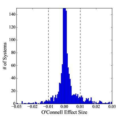
Figure 2: Histogram showing the OES distribution for the KEBC. The central peak at an OES of 0.00 rises to a value of 1,367 systems and is truncated for clarity. There are 26 additional systems with $|$OES$|>0.03$ not included in this figure for clarity. The dashed lines indicate the $|$OES$|=0.01$ cutoff defining our sample.

2.4 Selection Method: O’Connell Effect Size Determination

We tried several methods to produce our sample. We first tried manually selecting our sample based on visually inspecting KEBC light curves, but this method is inherently subjective and non-reproducible. We then tried using the automated detector Johnston et al. (2019) describes, as they made this detector to create our sample. However, due in part to the light curve scaling Johnston et al. (2019) used, it found over 70 systems that did not meet our criterion. Additionally, the detector did not find several other systems that we knew from visual inspection should be in our sample. Therefore, we developed a code that directly calculated the OES, which we used to select our sample.

First, we downloaded the short- and long-cadence Kepler data for each eclipsing binary from the KEBC website. Our code split each cadence’s data into 1,001 equally-spaced bins in phase space for $\phi\in[-0.5,0.5]$, where the bins for $\phi=-0.5$ and 0.5 contain the same data. It then calculated the weighted average flux $F$ for each bin using inverse-variance weighting (Hartung et al., 2008):

$$F=\frac{\sum_{i}{f_{i}/\sigma_{f_{i}}^{2}}}{\sum_{i}{1/\sigma_{f_{i}}^{2}}}$$ (1)

along with the error:

$$\sigma_{F}=\sqrt{\frac{1}{\sum_{i}{1/\sigma_{f_{i}}^{2}}}}$$ (2)

where $\sigma_{f_{i}}$ is the error of the $i$^th data point in the bin. We estimated the flux value for any phase bins without data by linearly interpolating between the nearest bins with data. The code introduced a phase shift setting the phase bin with the lowest average flux to $\phi=0$. The resultant light curve represents an averaged light curve for the system, an example of which is shown in Figure 1. Note that, throughout this work, we removed all data from KIC 9164694 with BJD in the ranges [2455309.2870355, 2455336.8939506] and [2455432.2188883, 2455552.5485149] to correct an apparent data processing issue wherein the flux values during these intervals were systematically reduced by $\sim$2%. We also removed a single outlier datum from KIC 8029708’s data. Finally, 160 KEBC systems have the flag QAM, which indicates that these systems’ amplitudes differ between Kepler quarters. Eighteen of these systems are in our sample. The KEBC corrected for this amplitude mismatch by rescaling the data to match between quarters, and we use this rescaled flux in our analysis. However, in at least one case (KIC 4474637), this rescaling did not correct the issue, and so this system exhibits significantly increased scatter in its data and its averaged light curve.

The code produced a smoothed version of the light curve by convolving each point in the averaged light curve with the immediately adjacent points. The convolution reduces the effect of data scatter and oscillations on the light curve, giving a more accurate measure of the OES. Since convolution in time space is equivalent to multiplication in frequency space (Press et al., 2007), we performed the convolution in frequency space after applying a discrete Fourier transform to the phased data. Our code multiplied the transformed data by the transformed convolution kernel 50 times in frequency space, equivalent to convolving the data 50 times in time space. It then transformed the data back into time space using the inverse discrete Fourier transform and measured the maximum value of this convolved curve on either side of the primary minimum. The difference between these two maxima is the OES. The OES is positive when the maximum after the primary eclipse is brighter than the one preceding it, and we say that a system with a positive OES has a positive O’Connell effect. Conversely, we say that a system where the maximum before the primary eclipse is brighter than the one following it has a negative O’Connell effect. We found the error of each bin in the convolved curve by convolving the errors given by Equation 2 in the same fashion as we convolved the averaged data. The error in the OES is then given by propagating the error of the bins used to determine the OES. The maxima difference data from this code provided the basis for the histogram in Figure 2. Because we determine the OES from the convolved curve, which is derived from the averaged light curve, this OES represents the average size of the O’Connell effect over the duration of Kepler’s observations.

This method for finding O’Connell effect binaries is viable only because we applied it to a set of known eclipsing binaries. If applied to a general population of stars, this method would find many non-eclipsing systems, such as pulsating variables and spotted stars. The KEBC therefore acts as a filter that allows this method to find O’Connell effect binaries. This method is also quite sensitive, and several systems near the $|$OES$|$ cutoff of 0.01 would cross that threshold when we would change our method. For instance, when we began using Equation 1 instead of the standard definition of the mean, three systems with $|$OES$|$ above the criterion threshold decreased to under it, while three systems under it increased to above it. This sensitivity to the precise method of determining the OES makes it more challenging to accurately reproduce our sample. It also explains why this method initially added systems to our sample that ultimately did not meet the criterion. To estimate the sensitivity of our method, we varied the cutoff by a small amount and determined the number of systems meeting the new cutoff. We found that varying the cutoff value by 0.0002 in either direction changed the sample size by about $\pm 5$ ($\pm 2.3\%$), while varying it by 0.001 changed the sample size by about $\pm 28$ ($\pm 13.2\%$).

Figure 3: Kepler short-cadence (left) and long-cadence (right) light curves of KIC 7667885. The system displays a negative O’Connell effect and at least one significant flare event.

It is also important to keep in mind that our averaging process removes information about the temporally varying properties of the system. The non-averaged OES changes in magnitude and even sign in several systems, as does the overall shape of the light curve. Removing this information simplifies the analysis of these systems but reduces the utility of the averaged light curve in studying temporal variation. We will analyze the temporal variation separately by looking at the eclipse timing variation (discussed further in Section 4.3).

2.5 Target Sample

Our final, complete sample consists of 211 systems found by our final OES determination code, 1 system (KIC 7667885) found in Ramsay et al. (2014), and 46 systems found using earlier methods, for a total of 258 systems. Our OES determination code showed that three additional systems met our criterion. Of these, KIC 7950964 is a duplicate entry of a system already in the sample (KIC 7950962), and KIC 9137819 appears to be an RR Lyrae variable and not an eclipsing binary. These two systems have since been removed from the KEBC (A. Prša 2021, private comm.). The third system, KIC 8456774, is a heartbeat star (Thompson et al., 2012), which is an eccentric binary that becomes tidally distorted at periapsis. KIC 8456774, like many heartbeat stars, does not appear to be eclipsing, and we do not consider it to have an O’Connell effect due to the fundamentally different origin of its asymmetry. Additionally, it is inappropriate to apply the phase offset we introduced to place the primary minimum at $\phi=0$ to non-eclipsing systems like KIC 8456774, and the OES without this phase offset is negligible. We do not include these three systems in our sample. We also do not include systems like KIC 11560447 that meet our criterion with their short-cadence data but not with their long-cadence data.

Kepler observed KIC 7667885 during quarters 14-17, but the KEBC does not include the system. Inspection of KIC 7667885’s short-cadence data from MAST indicated that it met our criterion. We detrended the single-aperture photometry (SAP) flux by fitting Legendre polynomials up to order 150 to continuous data blocks (defined as a set of data with no gaps longer than a day) and then dividing the flux by the fitted trend. We then normalized the data by dividing the flux by the median flux value of each data block. This method is similar to the one outlined in Section 4.2 of Slawson et al. (2011), which they used to produce the KEBC data. We determined a period of $0.314840\pm 0.000004$ d using the analysis of variance (Schwarzenberg-Czerny, 1989, 1996) method with the software Peranso. Figure 3 shows the resultant phased short- and long-cadence light curves. We did not determine the morphology parameter of KIC 7667885, nor did we perform an analysis of its ETV, but we otherwise fully incorporated the system into our sample.

One system in our sample, KIC 7879399, lies only 4” from another Kepler system, KIC 7879404. As a result of their proximity, these two systems’ data are blended, making it difficult to determine which one is the eclipsing binary. The first two releases of the KEBC (Prša et al. 2011 and Slawson et al. 2011) identified KIC 7879404 as the binary. The third release (Kirk et al. 2016 and Abdul-Masih et al. 2016), however, identified KIC 7879399 as the binary. C. Cynamon of the American Association of Variable Star Observers (AAVSO) observed these stars for us (C. Cynamon 2021, private comm.), and our analysis of his data conclusively confirms KIC 7879399 as the eclipsing binary.

Of the 258 systems in our sample, 46 selected before we finalized the selection method do not meet our criterion. We will describe these 46 marginal sample systems in a separate paper. The remaining 212 systems (the 211 KEBC systems found by our OES determination code and KIC 7667885, which our code also found when we added its processed data to the KEBC’s) constitute our core sample, which represents 7.3% of the systems in the KEBC. Table 1 lists all 258 systems in our complete sample.

3 Methodology

We used several methods to characterize the systems in our sample: determinations of the eclipse depth, the O’Connell Effect Ratio and Light Curve Asymmetry, the KEBC’s morphology parameter, and statistical analyses of the sample characteristics. The majority of these methods involved analyzing the phased Kepler data taken from the KEBC using our in-house Python codes.

3.1 Eclipse Depth Determination

The KEBC provides a value for the eclipse depth determined using the polyfit method described in detail in Appendix A of Prša et al. (2008). In brief, the polyfit uses a chain of piecewise smooth polynomials connected at dynamically determined knots to fit the light curve, therefore providing a smoothed version of the light curve. This procedure works for the majority of systems in the KEBC. Unfortunately, it fails to accurately measure the eclipse depth for a small number of systems in our sample, as shown in Figure 4 with KIC 9777984’s polyfits (note that Kirk et al. 2016 and the KEBC identify this system as KIC 9777987, while Abdul-Masih et al. 2016 identifies it as KIC 9777984). Furthermore, Kirk et al. (2016) states that the provided eclipse depths are approximate and only as accurate as the polyfits used to produce them.

We therefore needed to define our own method for determining eclipse depth. The convolved curve used to determine the OES consistently underestimates the depth of the eclipse, so we instead applied a Savitzky–Golay filter (Savitzky & Golay, 1964) of polynomial order 4 and window size 7 to each averaged light curve. We applied the filter in the same way we convolved the data in Section 2.4, the sole difference being in the kernel. We used SciPy’s savgol_coeffs function to determine the kernel values for the Savitzky–Golay curve. This procedure produced a curve that approximates the eclipse depth much better than the polyfits for KIC 9777984 – as Figure 4 shows – despite retaining more of a oscillatory pattern than the convolved curve. We found the Savitzky–Golay curve’s errors similarly to how we found the convolved curve’s errors. We take the smallest value of this curve to be the point of maximum eclipse, and the error of the corresponding bin is the eclipse depth error. A limitation of this method is that Algol-type systems with narrow eclipses can have their eclipse depths underestimated by 50% or more. Nevertheless, the Savitzky–Golay curve measures the eclipse depth more accurately than the Fourier curve (Section 3.2), particularly for some Algol-type systems like KIC 5700330 that lie outside of our sample. The Savitzky–Golay curve is also more accurate than the convolved curve in all but a few edge cases involving totally-eclipsing Algol-type systems.

Figure 4: Kepler light curve of KIC 9777984 showing three fits to the system: the KEBC’s original polyfit (green), the KEBC’s reconvolved polyfit (blue) that corrects for Kepler’s non-zero integration time, and our fit using the Savitzky–Golay filter (red). The Savitzky–Golay curve better fits KIC 9777984’s light curve and provides a more accurate measure of the eclipse depth for this system.

Establishing a proper reference point from which to measure the depth is a non-trivial matter. We rejected using either maximum as the reference point as it is uncertain which maximum (if either) is unaffected by the process causing the O’Connell effect. Communication with the KEBC team revealed that they face the same uncertainty about a proper reference point and noted that modeling the light curve provides the only robust way of determining eclipse depth (A. Prša 2020, private comm.), a procedure which is beyond the scope of this paper. Therefore, we used the KEBC’s normalized data and adopted a normalized flux value of unity to establish each system’s baseline flux. We then subtracted the flux value at the eclipse minimum from this baseline to find the eclipse depth. Slawson et al. (2011) details the normalization scheme used for the KEBC data, and it is “reasonable to assume that, for the most part, the data are median-normalized” (A. Prša 2020, private comm.).

3.2 O’Connell Effect Ratio and Light Curve Asymmetry

The O’Connell Effect Ratio (OER) and Light Curve Asymmetry (LCA) are two statistical measures introduced by McCartney (1999), who used them with phased light curves broken into $n$ equally-spaced phase bins. While originally introduced to characterize the O’Connell effect in W Ursae Majoris-type systems, OER and LCA are valid measures for all light curve classes. The original definitions given by McCartney (1999) are:

$$\text{OER}=\frac{\sum_{i=1}^{n/2}{I_{i}-I_{0}}}{\sum_{i=(n/2)+1}^{n}{I_{i}-I_{0}}}$$ (3)

and:

$$\text{LCA}=\sqrt{\sum_{i=1}^{n/2}{\left(\frac{I_{i}-I_{n+1-i}}{I_{i}}\right)}^{2}}$$ (4)

where $n$ is the number of phase bins, $I_{i}$ is the average intensity of the $i$^th bin, and $I_{0}$ is the minimum average intensity of the light curve. Note that the LCA should contain a normalization factor to account for the number of bins, i.e.:

$$\text{LCA}=\sqrt{\frac{1}{n}\sum_{i=1}^{n/2}{\left(\frac{I_{i}-I_{n+1-i}}{I_{i}}\right)}^{2}}$$ (5)

as in W09. W09 transformed these summations into integrals (taking $n\to\infty$) such that:

$$\text{OER}=\frac{\int_{0}^{1/2}{[I(\phi)-I(0)]~{}d\phi}}{\int_{1/2}^{1}{[I(\phi)-I(0)]~{}d\phi}}$$ (6)

and:

$$\text{LCA}=\sqrt{\int_{0}^{1/2}{\left(\frac{I(\phi)-I(1-\phi)}{I(\phi)}\right)^{2}}~{}d\phi}$$ (7)

where $I(\phi)$ is the $N$-term Fourier series representation of the light curve:

$$I(\phi)=\frac{a_{0}}{2}+\sum_{i=1}^{N}{[a_{i}\cos{(2\pi i\phi)}+b_{i}\sin{(2\pi i\phi)}]}$$ (8)

We use the integral formulation in this paper. Both OER and LCA assume that the secondary eclipse occurs at $\phi=0.5$, so systems with eccentric orbits have inaccurate OER values. The LCA, by contrast, interprets the eccentricity as an asymmetry in the light curve.

Figure 5: Averaged light curve of KIC 11347875 showing two Fourier series approximations of the system: the 50-term series used in this paper (solid red) and a 12-term series (dashed blue) similar to one Akiba et al. (2019) would use. The 50-term series follows the averaged data more closely than the 12-term series while not capturing the statistical scatter.

We chose to use a 50-term Fourier series based on a $\chi^{2}$ analysis of $N$ for our complete sample of 258 systems. Our code calculated the $\chi^{2}$ statistic by comparing the Fourier curve with $N$ coefficients to the averaged light curve of the system, where $N\in[2,500]$. This analysis indicated a median optimal $N$ of 59. We adopted an $N$ of 50 because we found that varying $N$ in the range $[40,60]$ changes the results little. Figure 5 compares our 50-term Fourier series of the core sample system KIC 11347875 to a 12-term Fourier series like those used in Akiba et al. (2019) and Hahs et al. (2020). Figure 5 demonstrates that 50 terms are sufficient to capture most large-scale features in the light curve without having so many terms that the series approximates small-scale statistical scatter.

We obtained our Fourier series by applying a discrete Fourier transform to the averaged light curve described in Section 2.4. Our code converted the resultant complex-valued coefficients $c_{i}$ to the Fourier series coefficients $a_{i}$ and $b_{i}$ using the equations:

$$a_{i} =\frac{2\text{Re}(c_{i})}{n}$$ (9a)

$$b_{i} =-\frac{2\text{Im}(c_{i})}{n}$$ (9b)

We use the resulting Fourier series to calculate the OER and LCA using Equations 6 and 7, respectively. We also use the $a_{i}$ coefficients to determine each system’s light curve class, as we describe in Section 3.3. The 50-term Fourier series is an excellent approximation of $\beta$ Lyrae- and W Ursae Majoris-type systems. However, it struggles to accurately represent several Algol-type systems, particularly those with sharp, narrow eclipses. Such systems dominate the long-period ($P>10$ d) population of the KEBC but are rare in our sample.

We based our error analysis on the method described in Akiba et al. (2019), but there were some differences caused by our use of fft, most prominently that all $a_{i}$ and $b_{i}$ coefficients with $i>0$ have the same error. This error is given by:

$$\sigma_{X}=\frac{\sqrt{2}}{n}\sqrt{\sum_{j=1}^{n}{\displaystyle\sigma_{x_{j}}^{2}}}$$ (10)

where $\sigma_{x_{j}}$ are the errors of each bin given by Equation 2. The error for $a_{0}$ is larger by a factor of $\sqrt{2}$. Our errors for OER and LCA are:

$$\begin{split}&\sigma_{\text{OER}}=\text{OER}\frac{\sigma_{X}}{2}\\ &~{}~{}~{}\times~{}\sqrt{\frac{N+2\sum_{i=1}^{N}{\left(\frac{1}{\pi i}\right)^{2}}}{\left[H\left(\frac{1}{2}\right)-H(0)\right]^{2}}+\frac{5N+2\sum_{i=1}^{N}{\left(\frac{1}{\pi i}\right)^{2}}}{\left[H(1)-H\left(\frac{1}{2}\right)\right]^{2}}}\end{split}$$ (11)

and:

$$\begin{split}\sigma_{\text{LCA}}&\approx\frac{\sigma_{X}}{\text{LCA}}\int_{0}^{1/2}{}\left[\left(\frac{I(\phi)-I(1-\phi)}{I(\phi)}\right)^{2}\right.\\ &~{}~{}~{}~{}~{}\left.\times~{}\sqrt{\frac{2\left(N+\frac{1}{2}\right)}{\left[I(\phi)-I(1-\phi)\right]^{2}}+\frac{N+\frac{1}{2}}{\displaystyle I(\phi)^{2}}}\right]~{}d\phi\end{split}$$ (12)

where:

$$\begin{split}H(\phi)&=\sum_{i=1}^{N}{\left[\frac{a_{i}}{2\pi i}\sin{(2\pi i\phi)}-\frac{b_{i}}{2\pi i}\cos{(2\pi i\phi)}\right.}\\ &~{}~{}~{}~{}~{}~{}~{}~{}~{}~{}~{}\left.\vphantom{\frac{b_{i}}{2\pi i}\cos{(2\pi i\phi)}}{}-{}a_{i}\phi\right]\end{split}$$ (13)

is the antiderivative of $I(\phi)-I(0)$.

3.3 Morphology Parameter and Light Curve Classification

Matijevič et al. (2012) introduced the morphology parameter (which we represent with the symbol $\mu$) to determine the morphology class of KEBC systems. They used local linear embedding (Roweis & Saul, 2000) to reduce the light curve’s polyfit representation (Prša et al., 2008) to a single, one-dimensional parameter. This parameter proved to correlate very well with their manually identified morphology class for most KEBC systems. They determined that $\mu\leq 0.5$ implied detached systems, $0.5<\mu\leq 0.7$ implied semi-detached systems, $0.7<\mu\leq 0.8$ implied overcontact systems, and $\mu>0.8$ implied ellipsoidal variables (non-eclipsing systems where the variation is due to the changing aspect of tidally distorted stars). They note, however, that the morphology parameter is a “best guess” at the morphology class and that system modeling can more accurately determine the morphology class. Nevertheless, we use the morphology parameter to estimate a system’s morphology class throughout this paper, and Table 1 lists each system’s morphology parameter.

Based on our own visual classification of the systems in our sample, we estimated that Algol-type systems have $\mu<0.6$, $\beta$ Lyrae-type systems have $0.6\leq\mu<0.75$, and W Ursae Majoris-type systems have $\mu\geq 0.75$. These boundaries agree with those in Matijevič et al. (2012), as Algol-type systems are generally detached or semi-detached, $\beta$ Lyrae-type systems can be of any morphological class, and W Ursae Majoris-type systems are predominantly overcontact (although detached and semi-detached eclipsing binaries, as well as ellipsoidal variables, may also appear as W Ursae Majoris-type systems).

In addition, we quantified the light curve classification using the Fourier coefficients obtained from Equation 9a. Our procedure is a modification of the one described in Section 3.2 of Akiba et al. (2019) and uses the following criteria to classify systems:

1. If $a_{4}<a_{2}(0.125-a_{2})$, the system is classified as an Algol-type system.

2. If $a_{4}\geq a_{2}(0.125-a_{2})$ and $|a_{1}/a_{2}|>0.25$, the system is classified as a $\beta$ Lyrae-type system.

3. If $a_{4}\geq a_{2}(0.125-a_{2})$ and $|a_{1}/a_{2}|\leq 0.25$, the system is classified as a W Ursae Majoris-type system.

Criterion 1 comes from Rucinski (1997) and is unchanged from Akiba et al. (2019), as are the first parts of Criteria 2 and 3. However, the second parts of Criteria 2 and 3 differ from Akiba et al. (2019), who instead used $|a_{1}|>0.05$ to define $\beta$ Lyrae-type systems and $|a_{1}|<0.05$ to define W Ursae Majoris-type systems. These criteria arise from W09’s observation that $a_{1}$ is proportional to the difference in eclipse depth. Unfortunately, $a_{1}$ does not contain any information about the eclipse depth ratio, which is the parameter related to the component temperature ratio (Kallrath & Milone, 2009). We introduced $a_{2}$ (which W09 notes is proportional to the light curve amplitude) to quantify the eclipse depth ratio.

We note that our sample likely contains several ellipsoidal variables. It is difficult to distinguish an ellipsoidal variable from an overcontact system due to their similar light curves. Preliminary modeling of four systems in our sample with PHOEBE v0.31a (Prša & Zwitter, 2005) shows that the morphology parameter is not wholly effective at identifying ellipsoidal variables. As an example, KIC 8285349 has $\mu=0.90$ but clearly shows an eclipse. Meanwhile, KICs 10815379 and 10979669 have $\mu=0.79$ and 0.83, respectively, but are non-eclipsing according to our models. Identifying and removing ellipsoidal variables would therefore require large-scale modeling of the sample systems, which is beyond the scope of this paper.

3.4 Statistical Analysis

To determine if our sample population was similar to the KEBC population as a whole, we performed the Kolmogorov–Smirnov test (K–S test; Kolmogorov, 1933; Smirnov, 1948) on the observational characteristics we studied. If the test statistic differs for a given characteristic, it suggests a potential link between that characteristic and a significant O’Connell effect. We expect the OES and $|$OES$|$ populations to differ due to how we defined our sample. We do not expect the distance populations to differ because the O’Connell effect should be independent of distance.

We determined correlations between characteristics using Spearman’s $\rho$ coefficient (Spearman, 1904), as in D84. We also used Kendall’s $\tau$ coefficient (Kendall, 1938) as a second test of correlation. Our decision to use both coefficients stemmed from research showing that the two measures complement each other (Xu et al., 2013). Unlike O51 and D84, we did not use Pearson’s r coefficient due to its sensitivity to outliers and assumption of a linear correlation. We tested six functional forms for each correlation using SciPy’s implementation of orthogonal distance regression (ODR; Boggs et al., 1987) to determine the best fit to the correlation. The functional forms we tested were linear, quadratic, exponential, logarithmic, power law, and inverse.

In order to test the robustness of our correlation analysis results, we performed a bootstrapping procedure on our sample. Our code randomly selected 20 subsets of 40 systems from our core sample (and 400 systems from the KEBC) and computed the Spearman’s $\rho$ coefficients for each subset. We considered a correlation robust if at least 19 of the 20 subsets recovered the correlation.

4 Results

We now present a detailed summary of various characteristics of the core sample, specifically the light curve characteristics (distributions of eclipse depth, OES, and positive and negative OESs) and physical characteristics (spatial, luminosity, temperature, and period distributions). Determining the characteristic distributions of the underlying population allows us to make inferences about the physical processes underlying the O’Connell effect. We also discuss the results of our analysis of the ETV, OER, and LCA. Finally, we present several system classes in our sample that show peculiar features in their light curves aside from the O’Connell effect. These features include changes in the light curve over time, asymmetric minima, and concave-up regions. In the figures in Sections 4 and 5, the distribution or data set labeled “Core Targets” includes all 212 core sample systems, while the distribution or data set labeled “KEBC Systems” includes the core sample (except KIC 7667885) and the rest of the KEBC. In this section, we use the comparative subset of the KEBC discussed in Section 2.2, which excluded four systems: KIC 5217781, a long-period system with severe data corruption, KIC 7667885, due to it not being in the KEBC, and KICs 7950964 and 9137819, due to their removal from the KEBC (as explained in Section 2.5).

4.1 Light Curve Characteristics

We determined several characteristics from analyzing the Kepler photometry of the KEBC systems: light curve class, OES, the proportion of positive and negative O’Connell effects (defined in Section 2.4), primary eclipse depth, and the ratio between $|$OES$|$ and the primary eclipse depth. This section discusses the range and distribution of these characteristics. Using the method described in Section 3.3, we classified 54 systems (25% of our sample) as Algol-type, 40 (19%) as $\beta$ Lyrae-type, and 118 (56%) as W Ursae Majoris-type. This distribution strongly differs from the KEBC’s, wherein 1,990 (68%) are Algol-type, 250 (9%) are $\beta$ Lyrae-type, and 679 (23%) are W Ursae Majoris-type.

The largest OES in our sample is KIC 11347875, which has an OES of $-0.265$ in units of normalized flux. However, KIC 1134785 is an unusual system in that one of its inter-eclipse maxima is instead a minimum. Therefore, it lacks an O’Connell effect in the traditional sense described in Section 1. We discuss KIC 11347875 further in Section 4.5.4. The largest OES among systems with a more traditional O’Connell effect is KIC 9935311, with an OES of 0.115. A clear majority of systems (147, or 69% of the sample) show a positive O’Connell effect, where the brighter maximum is the one following the primary eclipse. We discuss the implications of this preference for a positive O’Connell effect in Section 5.2.1.

The primary eclipse depth ranges from 0.025 (KIC 8190491) to 0.916 (KIC 9101279) in units of normalized flux. Figure 6 shows the ratio between $|$OES$|$ and the primary eclipse depth for the core sample and the KEBC. We have determined that the overwhelming majority of systems with a ratio above 0.5 are heartbeat stars, a type of binary discussed in Section 2.5. The only system in our sample among such high ratio systems is the aforementioned non-heartbeat star KIC 11347875, which has a ratio of 0.658.

Figure 6: Histogram comparing the ratio $|$OES$|$/primary eclipse depth for our core sample (solid red) and all entries in the KEBC (dashed grey). Systems with a ratio above 1 are not displayed. Core sample systems have a larger ratio on average than other KEBC systems.

4.2 Physical Characteristics

We determined several physical characteristics from the published information on the KEBC: distance, luminosity, period, temperature, and spectral type. This section focuses on these characteristics’ distributions for our core sample and the KEBC. We also discuss our sample’s color-magnitude diagram and references that indicate the presence of flares, spots, or mass transfer in our systems. Figure 7 shows a histogram of the distances derived from Gaia parallaxes (Bailer-Jones et al., 2021) for our sample, along with the distance distribution for the KEBC. These two distributions appear similar. Figure 8 shows a histogram of the luminosity distribution in our sample and the KEBC, and we note that our sample’s systems are less luminous on average than those in the KEBC. Figure 9 shows a histogram of the period distribution for our sample and the KEBC. We obtained these periods directly from the KEBC, and Figure 9 has a logarithmic scale to capture the KEBC’s wide range of periods. Figure 9 shows that our sample has a similar distribution for $P\leq 0.5$ d, but the proportion of systems with longer periods drops precipitously.

Figure 7: Histogram comparing the implied distances for the 212 core sample targets (solid red) and 2,860 of 2,862 entries in the KEBC (dashed grey) with Gaia EDR3 parallaxes (excluding two systems with $\text{d}>9,\!000$ pc). Our core sample’s distances range from 210 pc (KIC 7671594) to 7,743 pc (KIC 4474637). The two distributions are similar.

Both the KEBC and Gaia DR2 (Gaia Collaboration et al., 2018) provide temperatures for most of our targets based on their colors. The KEBC temperatures range from 3,717 K (KIC 7671594) to 8,540 K (KIC 10857342), while the Gaia temperatures range from 3,808 K (KIC 7671594) to 8,540 K (KIC 10857342). The Kepler and Gaia temperatures are similar for the systems in our sample. Nine target systems do not have a Kepler temperature, while seven do not have a Gaia temperature. We chose to use Gaia as our primary source of temperature in light of the more complete coverage Gaia provides.

Frasca et al. (2016) provides spectral types for a handful of target systems determined using optical spectra (although they do not state if they assumed solitary stars during their data processing), and the main-sequence spectral types range from K5 (KIC 12109575) to A2 (KIC 8904448). There are eleven systems with an explicit non-main-sequence spectral type listed in Table 1. Ramsay et al. (2014) spectrally classified KIC 7667885 and KIC 9786165 as “mid G” systems. We used the online table of photometric colors periodically updated by Dr. Eric Mamajek (Pecaut & Mamajek, 2013) in combination with the Gaia colors provided by EDR3 to expand the spectral classification to the entire sample. While this does not account for interstellar reddening, evolutionary stage, or color blending of the binary components, it provides a first approximation estimate of the spectral class for all systems in our sample, which Table 1 also lists. By this estimate, the spectral types of our sample range from M2.5 V (KIC 7671594) to A7 V (KIC 10857342).

Figure 8: Histogram comparing the luminosities for the 212 core sample targets (solid red) and all 2,862 entries in the KEBC (dashed grey) with Gaia EDR3 parallaxes. Note the logarithmic scale of the x-axis. Our core sample’s calculated luminosities range from 0.02 L_$\odot$ (KIC 7671594) to 50.25 L_$\odot$ (KIC 5820209). Systems in our sample are less luminous on average than other KEBC systems.

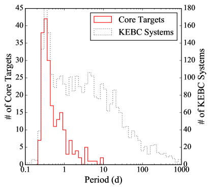
Figure 9: Histogram comparing the periods for all 212 core sample targets (solid red) and all 2,915 entries in the KEBC (dashed grey) with a period below 1,000 d. Note the logarithmic scale of the x-axis. Our core sample’s orbital periods range from 0.234 d (KIC 6050116) to 9.752 d (KIC 6197038). The distributions are similar under 0.5 d, but our sample’s long-period population decreases much more quickly than the KEBC’s.

Figure 10 shows a color-magnitude diagram using Gaia EDR3 data. The marker color and shape show the light curve classification for each system determined using the criteria given in Section 3.3. Figure 10 shows the Kepler selection bias discussed in Batalha et al. (2010) and Section 2.1, as there are few systems with a Gaia color index $\text{BP}-\text{RP}\geq 1.5$ or $\text{BP}-\text{RP}\leq 0.5$. Our sample’s distribution in Figure 10 is similar to the KEBC’s along most of the main sequence, suggesting that our sample is not strongly biased beyond Kepler’s selection function. Additionally, only two clear giants exist in our sample (KICs 5820209 and 9489411, although the former’s 0.656-day period is incongruent with containing a giant because such a period with two 1 M_$\odot$ stars implies a maximum star size of only $\sim$2.5 R_$\odot$).

Numerous systems in our sample are thought to have observed flares (57% of the sample; Balona, 2015; Gao et al., 2016; Davenport, 2016) or be spotted (42%; Tran et al., 2013; Balaji et al., 2015). Table 1 lists these systems with reference numbers 1-3 and 4-5, respectively, and the flags F and S, respectively. Kouzuma (2018) found evidence for mass transfer in 22 (10%) systems in our sample. Table 1 lists these systems with reference number 6 and the flag M. Therefore, our sample consists mainly of solar-type main-sequence stars with evidence for flares, spots, or mass transfer in 148 (70%) sample systems.

4.3 Eclipse Timing Variations

Eclipse timing variation (ETV) measures how much the primary and secondary eclipses times vary from their theoretical values calculated assuming a constant period. ETV patterns reveal apparent period changes due to light travel time effects (LTTEs) caused by a third body, along with actual period changes due to effects such as mass transfer. Mass transfer creates a parabolic signal (as Figure 11’s left panel shows), while an LTTE creates a sinusoidal signal with a period equal to the third body’s orbital period (as Figure 11’s right panel shows). For this paper, we use the ETV data published by Conroy et al. (2014), a paper describing the ETVs of KEBC systems with morphology parameters between 0.5 and 1.0. Conroy et al. (2014) distinguished a parabolic signal from a long-period sinusoidal signal using the Bayesian Information Criterion (Schwarz, 1978). Only three core sample systems (KICs 5020034, 6044064, and 7696778) show a parabolic ETV signal, while none from our marginal sample do. By contrast, forty core sample systems and seven marginal sample systems show a sinusoidal signal. Furthermore, forty-seven core sample systems and seven marginal sample systems show an “interesting” ETV, meaning it has a pattern that does not clearly fit into the other two categories.

Figure 10: Color-magnitude diagram showing the 212 systems in the core sample overplotting the rest of the KEBC systems. The Gaia color is plotted against the absolute magnitude in Gaia’s G band. The systems are color coded according to their light curve class. Most of our sample are solar-type main-sequence stars.

Figure 11: Eclipse timing variation of KIC 7696778 (left) and KIC 8904448 (right). KIC 7696778’s ETV has a parabolic shape, consistent with a linear change in period caused by mass transfer between components, while KIC 8904448’s ETV has a sinusoidal shape, consistent with LTTEs caused by a third body orbiting the binary.

The twenty-two core sample systems Kouzuma (2018) cited as undergoing mass transfer do not include the three systems Conroy et al. (2014) flagged with a parabolic ETV. However, the KEBC flagged sixteen of these twenty-two systems with a sinusoidal or interesting ETV, and visual inspection of their ETVs suggests that, aside from KIC 2437038, their signals are roughly parabolic. Figure 12 shows the ETV of two systems Kouzuma (2018) references: KIC 6791604 (flagged as interesting) and KIC 11924311 (flagged as sinusoidal). To further investigate our core sample’s ETVs, we applied a digital Butterworth filter (Butterworth, 1930) of order one to the ETV data using SciPy’s butter function to reduce noise from effects such as starspots. The sampling frequency is the orbital frequency, and we set the cutoff frequency to five cycles over the system’s observation span, thus removing signals such as starspot modulation that recur more than five times during Kepler’s observations. Due to the need for continuous sampling, we removed any system with an observation gap longer than 20 d, leaving a sample of 122 core sample systems. We fit a parabola to each system’s filtered data using SciPy’s curve_fit function and calculated the $R^{2}$ value of the fit. Thirteen systems (11% of the 122 investigated systems) have $R^{2}\geq 0.9$, while 25 systems (20%) have a less-stringent $R^{2}\geq 0.8$ (for reference, KIC 6791604’s ETV – shown in Figure 12’s left panel – has $R^{2}=0.895$). We regard these 25 systems as having an ETV that is not incompatible with being parabolic. Because these 122 systems form an unbiased subset of our core sample, we expect the same percentage of core sample systems to show a possibly parabolic ETV. Therefore, we estimate that up to 43 core sample systems show evidence of mass transfer in their ETV, making mass transfer a plausible, if rare, cause of the O’Connell effect.

Figure 12: Eclipse timing variation of KIC 6791604 (left) and KIC 11924311 (right). KIC 6791604 was flagged with an interesting ETV while KIC 11924311 was flagged as a sinusoidal ETV, but both are consistent with a roughly parabolic ETV as well.

4.4 O’Connell Effect Ratio and Light Curve Asymmetry

Figures 13 and 14 compare the OES to the OER (Equation 6) and the LCA (Equation 7), respectively. The data labeled “Non-Core Systems” include all KEBC systems not in the core sample, excluding KIC 5217781. Our analysis found many systems with an OES of $\sim$0 but OER $\neq 1$ or LCA $\neq 0$, producing significant vertical scatter in Figures 13 and 14. Systems in this scatter region of Figure 13 are low-amplitude (total change in flux $\Delta F\lesssim 0.03$) binaries with an OES that is large relative to their eclipse depth but small on an absolute scale. In Figure 14, the scatter region also includes long-period eccentric binaries. We removed a single data point from KICs 9701423 and 10614158 to avoid a nonphysical negative OER, although the low-amplitude system KIC 6948480 retains a negative OER. We excluded the two systems with $|$OES$|>0.1$ (KICs 9935311 and 11347875) from Figures 13 and 14 for clarity. The figures do not plot errors because they are too small to see at this scale for most systems.

Figure 13 shows a strong correlation between the OER and OES. This correlation is unsurprising because both measures account for the different amounts of light under both maxima, albeit in different ways. McCartney (1999) notes that the presence of a constant, third source of light contaminating the data will reduce the OES. However, the OER is not affected by third light due to subtracting the minimum flux value of the light curve. Therefore, the OER provides a more consistent measure of the O’Connell effect in this respect. On the other hand, the OER calculation method also means that the OER will be significant for systems like KIC 8912911 and KIC 10905824 with O’Connell effects that are large relative to their eclipse depth but small on an absolute scale. Based on this, we believe that the OER is ill-suited to describe the O’Connell effect in a general population of eclipsing binaries but is applicable to a subset of binaries with amplitudes larger than $\sim$0.01 in normalized flux.

Figure 14 shows that most of our sample lies along lines with slopes of $\pm$0.5 that meet at the origin. Many systems lie above these lines, but none lie significantly below them, implying that the O’Connell effect produces an LCA at least half as large as the OES. The LCA is also clearly sensitive to asymmetries aside from the O’Connell effect, as seen by the vertical scatter mentioned earlier. Many systems in this scatter (like KIC 10909274) are long-period systems with eccentric orbits, implying that the LCA is sensitive to unevenly-spaced eclipses. Therefore, the LCA serves as a good measure of a light curve’s asymmetry, but its sensitivity to other asymmetries means that it should not be relied on to detect the O’Connell effect.

4.5 Systems Showing Peculiar Features

Figure 13: Plot comparing the OER to the OES. Core sample targets are shown in red diamonds and non-core sample systems in black circles. KICs 9935311 and 11347875 are excluded for clarity.

Figure 14: Plot comparing the LCA to the OES. Core sample targets are shown in red diamonds and non-core sample systems in black circles. KICs 9935311 and 11347875 are excluded for clarity.

Four system classes showing peculiar features are present in our sample: those displaying significant temporal variation, those with an asymmetric minimum, those with a concave-up region in their light curves, and a white dwarf. Systems can belong to multiple classes. We have chosen an exemplar system to serve as an identifier for each class for the purpose of categorization. We discuss each class and identify characteristics systems in each class share. Future work will discuss each of these classes more in-depth. In Section 4.5, our discussion also includes systems from the marginal sample defined in Section 2.5.

4.5.1 KIC 7433513: Temporally Varying Systems

KIC 7433513 and systems like it (labeled with the flag TV in Table 1) display strong temporal variation in their light curves. Figure 15 shows KIC 7433513’s phased light curve using all Kepler data, clearly showing the significant data scatter caused by the temporal variation. Figure 16 shows 10-day time slices of KIC 7433513’s Kepler data separated by a few months, along with the Barycentric Julian Date (BJD) for the midpoint of each time slice. The system changes drastically even over these short timescales. It is difficult to rigorously quantify the number of these systems in our sample because there is a continuum between systems with stable light curves like KIC 5282464 (Figure 1) and systems like KIC 7433513. However, we estimate that about 20% of our core sample and about 65% of our marginal sample exhibits strong temporal variation. Three further examples from our sample are KICs 2569494, 3659940, and 9137992. Systems displaying this temporal variation are among our sample’s cooler systems, with the hottest (KIC 8294484) estimated at 5,760 K. Kunt & Dal (2017) described KIC 7885570 – a system from our marginal sample showing strong temporal variation – as an RS Canum Venaticorum variable. The stars in these systems have active chromospheres that produce large spots, and the evolution of these spots is a plausible source for the observed temporal variation.

4.5.2 KIC 9164694: Asymmetric Minima Systems

KIC 9164694 and systems like it (labeled with the flag AM in Table 1) contain an asymmetric minimum, as seen in Figure 17’s left panel showing KIC 9164694’s light curve. This asymmetry is rather subtle, and in KIC 9164694’s case, is best described as looking like someone has taken their finger and “pushed” the light curve upward and leftward in the region just to the right of minimum light. Asymmetric minima are a rarely discussed feature seen in some eclipsing binary systems, including RY Scuti (Djurašević et al., 2008), GR Tauri (Zhang et al., 2002), AG Virginis (Pribulla et al., 2011), and NSVS 7322420 (Knote et al., 2019). Asymmetries can appear in the primary minimum (as in KIC 9164694) or the secondary minimum (as in KIC 9717924; see Figure 17’s right panel). About 13% of our sample displays an asymmetric minimum in either eclipse. There appear to be two sets of asymmetric minima systems: those showing strong temporal variation (like KIC 7433513), and those showing comparatively little (like KICs 9164694 and 9717924). We focus on the latter set for this class, which consists of the marginal sample system KIC 5283839 and 15 core sample systems: KICs 2159783, 2449084, 6205460, 8248967 (according to a 20-term Fourier series), 8696327, 8822555, 8842170, 9164694, 9283826, 9717924, 9786165 (with short-cadence data only), 10528299, 10861842, 11395645, and 11924311. These 16 are among our sample’s hotter systems, with nearly half having a temperature over 6,000 K, and most show minimal temporal variation. We distinguish this asymmetry from what older literature like Brownlee (1957) and van’t Veer (1973) call an asymmetric minimum, as the latter asymmetry occurs closer to the eclipse’s beginning and end. By contrast, what we call an asymmetric minimum occurs around the eclipse’s center.

Figure 15: Kepler light curve of KIC 7433513 showing significant scatter caused by temporal variation.

Figure 16: Ten-day slices of phased Kepler data for KIC 7433513 separated by several months, showing the significant changes in the light curve over time. The number in each time slice’s subplot is the BJD for the midpoint of that time slice.

Figure 17: Averaged light curves of KIC 9164694 (left) and KIC 9717924 (right) showing an asymmetric primary and secondary minimum, respectively.

The most striking similarity between these systems is that all known asymmetric minima systems exhibit total eclipses. Total eclipses occur when one star is fully occluded during an eclipse and are distinguished by flat-bottomed or nearly flat-bottomed minima. It is unclear why asymmetric minima are only found in totally eclipsing systems and not in partially eclipsing systems. One hypothesis is that spots near one component’s poles cause the asymmetry. Another is that the change in flux causing the asymmetry is small enough that it is only detectable during totality, when the flux is nearly constant. We describe these two possibilities in the next two paragraphs. Some systems with total eclipses and a significant O’Connell effect do not show an asymmetric minimum, such as KIC 8386048. Additionally, some totally eclipsing systems with no O’Connell effect show an asymmetric minimum, such as the non-sample system KIC 8265951.

One difference between partially and totally eclipsing binaries is that parts of both stars are always visible for partially eclipsing systems. These regions of persistent visibility occur near each star’s visible pole. By contrast, one star is fully occluded in totally eclipsing systems, making it impossible for regions on that star to be persistently visible. Therefore, features near the poles (like spots) can be occluded in totally eclipsing systems but not partially eclipsing systems. BinaryMaker3 (BM3) tests showed that both polar and equatorial spots could produce an asymmetric minimum, however.

Our BM3 testing also indicated that the effect is strongly dependent on the presence of total eclipses. Figure 18 shows that a one-degree change in inclination is enough to transform a largely symmetrical eclipse into a significantly asymmetric one. Therefore, another hypothesis is that total eclipses are a prerequisite for a significant minimum asymmetry. We posit that a feature on one component, which we will call a hot starspot or spot, causes the asymmetry via its changing aspect. The spot must be azimuthally offset from the plane both 1.) perpendicular to the orbital plane and 2.) containing both stellar centers to produce an asymmetric minimum. The change in flux caused by the spot’s changing aspect is small compared to the change caused by the eclipsed star being covered (or uncovered) during the eclipse’s partial phase. Therefore, the large change in flux during the partial phase prevents the spot from creating a significant asymmetry. During the almost flux constant total phase, however, the small change in flux caused by the spot’s changing aspect has no other change in flux to compete with and can produce a significant asymmetry. Therefore, under our starspot model, asymmetric minima imply total eclipses.

Figure 18: Light curves of four eclipsing binary models detailing the area around the primary minimum. Parameters for all four models are identical except for inclination. The asymmetry grows significantly more pronounced as the system changes from partially eclipsing ($i=74,~{}75^{\circ}$) to totally eclipsing ($i=76,~{}77^{\circ}$), demonstrating the asymmetry’s strong dependence on total eclipses.

4.5.3 KIC 10544976: The White Dwarf

Figure 19: Averaged (left) and Kepler (right) light curves of KIC 10544976 using short-cadence data showing important features, including the sharp primary eclipse and numerous flares. The right panel also plots the averaged light curve in grey for comparison.

KIC 10544976 (labeled with the flag WD in Table 1) is unique within our sample as it is the only system containing a degenerate component. The lack of white dwarfs in our sample is unsurprising because white dwarfs were not priority targets for Kepler. Almenara et al. (2012) identifies the system as consisting of a DA white dwarf primary and an M4 V secondary in an 8.4-hour orbit. The left panel of Figure 19 displays KIC 10544976’s short-cadence average light curve, showing that the system has a very sharp, well-defined primary eclipse and no secondary eclipse. The red dwarf companion produces many flares, as Figure 19’s right panel shows. We consider this system to have a non-traditional O’Connell effect because the observed flux increases monotonically after the primary eclipse until phase $-0.35$. Therefore, the light curve lacks two inter-eclipse maxima to measure a difference between. KIC 10544976 has an OES of $-0.0096$, placing it within our marginal sample near the core sample cutoff.

4.5.4 KIC 11347875: Concave-Up Systems

KIC 11347875 has the largest measured O’Connell effect in our sample, but its light curve has an unusual appearance shared with six systems in the sample (labeled with the flag CU in Table 1). Figure 20 shows that KIC 11347875’s light curve is concave-up after the primary minimum, giving the system the appearance of an eclipsing signal superimposed on a rough sinusoid. Figure 5 shows an enlarged view of KIC 11347875’s concave-up region. As with KIC 10544976, the lack of inter-eclipse maxima indicates that the system has a non-traditional O’Connell effect. Gao et al. (2016) identifies KIC 11347875 as containing two late-type red giants based on effective temperature and surface gravity estimates, although our luminosity estimate from Gaia EDR3 data suggests a total luminosity of only 1.306 L_$\odot$. Six systems (KICs 5300878, 6044064, 6197038, 6697716, 7671594, and 9119652) show a similar concave-up region, as do some temporally varying systems like KIC 8479107 during some time intervals. However, KIC 11347875 is by far the most extreme example. All systems exhibiting a concave-up region are quite cool ($T<5,\!100$ K), have a longer orbital period ($P>1.2$ d), and show flares.

5 Analysis & Discussion

We now present a graphical representation of the correlations between the characteristics we studied (except distance and luminosity). We further discuss several correlations and their implications on the study of the O’Connell effect, with a focus on correlations involving OES, eclipse depth, and the morphology parameter.

5.1 Characteristic Trends

Figures 21, 22, and 23 show corner plots comparing period, OES, Gaia temperature, Gaia BP – RP color index, morphology parameter, absolute Gaia G magnitude, and primary eclipse depth. We chose the plot limits for clarity and, as such, the OES plots exclude KICs 9777984, 9935311, and 11347875. The banding seen in the temperature plots (most prominent in Figure 23’s right column) is a known issue with Gaia DR2 data (Andrae et al., 2018). The banding seen in the morphology plots (most prominent in the KEBC data of Figure 23’s top-center panel) is a quantization effect due to the morphology parameter being given to only two decimal places.

Figure 20: Averaged light curve of KIC 11347875 the system’s concave-up region following the primary eclipse.

Figures 21-24 used the trend subset of the KEBC discussed in Section 2.2, which excluded systems for two reasons: to analyze our sample without raising Python errors and not have results be affected by invalid parameter values. We excluded a given system because either it had no Gaia parallax data (43 systems, plus 1 system without a known Gaia EDR3 identifier), multiple entries in the KEBC (11 systems, 24 total entries), or had $\mu=-1$, indicating that the KEBC team could not assign a valid morphology parameter to the system (174 systems). We also explicitly excluded KICs 5217781, 7667885, 7950964, and 9137819, as in Section 4. These removals reduced the KEBC’s size to 2,678 systems. While we removed these 228 systems (241 entries) from our KEBC analysis in Section 5.2, we did not remove any from our core sample analysis.

5.2 Statistical Analysis

Table 2 gives the results of the K–S test described in Section 3.4. The K–S statistic describes the degree of difference between the populations the two samples were drawn from. The p-value indicates how compatible the K–S test results are with the null hypothesis that the two samples were drawn from the same population. We expected the significantly different OES distributions as we are looking at the wings of the distribution shown in Figure 2. This difference is intended by design as it was how we defined our sample. We also expected the distance distribution similarity, reinforced by Figure 7, because a phenomenon that should not depend on distance differentiates the samples. There is no reason to expect spatial differences between the two samples, and any biases in spatial distribution are due to biases in the Kepler sample. The remaining characteristics in Table 2 are of greater interest as the results point to possible underlying connections between those characteristics and the O’Connell effect.

Table 2: Kolomgorov–Smirnov Test Results

Characteristic	K–S Statistic	p-Value
O’Connell Effect Size	0.604	¡0.001
$|$O’Connell Effect Size$|$	0.871	¡0.001
Primary Eclipse Depth	0.398	¡0.001
Morphology Parameter	0.242	¡0.001
Temperature	0.277	¡0.001
Distance	0.092	0.080
Absolute Magnitude	0.285	¡0.001
Period	0.274	¡0.001

Table 3 gives the results of our correlation analysis described in Section 3.4. Kendall’s $\tau$ coefficients are uniformly smaller than Spearman’s $\rho$ coefficients and indicate the same correlations, so Table 3 presents only Spearman’s $\rho$ coefficients for the sake of brevity. The coefficient describes the correlation’s strength, while the p-value indicates how compatible the results of the Spearman test are with the null hypothesis that the characteristics are uncorrelated. We consider two characteristics correlated if $|\rho|\geq 0.1$ – consistent with D84 – and strongly correlated if $|\rho|\geq 0.2$. Characteristic pairs have their values bolded whenever they are correlated for a given sample. Table 3 also lists how many of the 20 random subsets produced by our bootstrapping procedure (described in Section 3.4) showed a correlation for each characteristic pair. Several correlations, such as the one between distance and absolute magnitude, are expected and serve as validations of our correlation analysis. We do not discuss such expected correlations despite their robustness as they are present for reasons unrelated to the O’Connell effect.

Table 3: Spearman’s $\rho$ Test Results

Characteristic	Characteristic	Core Sample					KEBC
One	Two	Coeff.		p-Value		Surv.	Coeff.	p-Value	Surv.
Informative O’Connell Effect Results
OES	Temperature	0.385	¡0.001	20	0.020	0.423	0
OES	Morphology	-0.148	0.032	16	0.024	0.326	0
OES	Absolute Mag.	-0.286	¡0.001	19	0.033	0.183	2
OES	Distance	0.218	0.001	17	-0.012	0.641	0
OES	Period	0.212	0.002	17	-0.069	0.005	4
Eclipse Depth	Morphology	-0.489	¡0.001	20	-0.158	¡0.001	18
Absolute Mag.	Period	-0.609	¡0.001	20	-0.370	¡0.001	20
Other Results
OES	Eclipse Depth	0.033	0.628	13	0.124	¡0.001	12
$|$OES$|$	Eclipse Depth	0.136	0.048	10	0.573	¡0.001	20
$|$OES$|$	Morphology	-0.055	0.428	10	0.210	¡0.001	20
$|$OES$|$	Temperature	-0.025	0.726	9	-0.213	¡0.001	19
$|$OES$|$	Distance	0.044	0.524	9	0.010	0.687	0
$|$OES$|$	Absolute Mag.	-0.027	0.696	11	0.236	¡0.001	20
$|$OES$|$	Period	0.046	0.506	8	-0.366	¡0.001	20
Eclipse Depth	Temperature	-0.039	0.575	9	-0.091	¡0.001	10
Eclipse Depth	Distance	0.057	0.405	10	0.071	0.004	6
Eclipse Depth	Absolute Mag.	-0.004	0.955	12	0.110	¡0.001	13
Eclipse Depth	Period	0.054	0.432	12	-0.084	¡0.001	10
Morphology	Temperature	0.113	0.109	12	0.196	¡0.001	20
Morphology	Distance	-0.148	0.032	13	0.025	0.317	1
Morphology	Absolute Mag.	0.065	0.350	12	-0.156	¡0.001	19
Morphology	Period	-0.591	¡0.001	20	-0.562	¡0.001	20
Temperature	Distance	0.245	¡0.001	17	0.139	¡0.001	19
Temperature	Absolute Mag.	-0.705	¡0.001	20	-0.695	¡0.001	20
Temperature	Period	0.248	¡0.001	16	0.236	¡0.001	20
Distance	Absolute Mag.	-0.512	¡0.001	20	-0.364	¡0.001	20
Distance	Period	0.348	¡0.001	20	0.100	¡0.001	8

We found that seven of the characteristic pairs we studied provided more insight into the O’Connell effect than the remaining ones. Table 3 highlights these seven pairs (OES and temperature, OES and morphology parameter, OES and absolute magnitude, OES and distance, OES and period, eclipse depth and the morphology parameter, and absolute magnitude and period). The bootstrapping procedure discussed in Section 3.4 guided our choice in which characteristic pairs were important: five of these pairs are robust and the other two are nearly so. These levels of robustness further raises our confidence in the results we present. Our discussion in Sections 5.2.1-5.2.4 focuses primarily on these characteristic pairs, along with several trends visible in Figures 21, 22, and 23. These trends include the lack of core systems with morphology parameters between 0.6 and 0.7 in the morphology panels, the clustering of systems along the right edge of Figure 22’s center panel, and the stark contrast between the positive and negative O’Connell effect systems’ temperature distributions in Figure 21’s center panel.

Figure 21: Corner plot showing the correlations between three characteristics of interest (period, OES, and temperature) and OES, temperature, and Gaia color. Core sample targets are shown in black while non-core KEBC systems are shown in grey. A few outlier systems have been removed from the OES plots for clarity (see discussion in text). Note the logarithmic x-axis of the period plots.

Figure 22: Corner plot showing the correlations between three characteristics of interest (Gaia color, morphology parameter, and primary eclipse depth) and morphology parameter, primary eclipse depth, and absolute Gaia G magnitude. Core sample targets are shown in black while non-core KEBC systems are shown in grey.

Figure 23: Corner plot showing the correlations between three characteristics of interest (period, OES, and temperature) and morphology parameter, primary eclipse depth, and absolute Gaia G magnitude. Core sample targets are shown in black while non-core KEBC systems are shown in grey. A few outlier systems have been removed from the OES plots for clarity (see discussion in text). Note the logarithmic x-axis of the period plots.

Our initial analysis of the KEBC found strong correlations between the OES and both period and the morphology parameter. Our inclusion of many long-period and well-detached systems that are fundamentally different from our sample’s systems strengthened these correlations. As a result of these fundamental differences, we considered these initial correlations less relevant to our study. Therefore, our final KEBC analysis used the analysis subset of the KEBC discussed in Section 2.2, which, in addition to the systems excluded in the earlier subsets, excluded systems with $P\geq 10$ d (690 systems) or $\mu\leq 0.3$ (1,018 systems), leaving only 1,639 KEBC systems. As in Sections 4 and 5.1, we removed no systems from our core sample analysis, and the KEBC population includes the core sample (except KIC 7667885). Our analysis considers both OES and $|$OES$|$.

5.2.1 O’Connell Effect Size

The OES (as defined in Section 2.4) reflects the difference in brightness at the two maxima, which in turn depends on the brightness difference between the leading and trailing hemispheres of each star. We gave particular focus to correlations and trends involving the OES because it defined our sample and is the characteristic most directly related to the O’Connell effect. This section discusses OES and $|$OES$|$ correlations with the other characteristics we studied. It also discusses the differences between the OES and $|$OES$|$ correlations.

Figure 21’s center panel comparing OES and temperature shows that a negative O’Connell effect, wherein the brighter maximum occurs before the primary minimum, mainly occurs in systems with $T<6,\!000$ K. Thirty-four (23% of 143 systems with a Gaia temperature) positive O’Connell effect systems have a temperature above 6,000 K, while only two (3% of 62 systems) negative O’Connell effect systems do. Furthermore, one of the two hot negative O’Connell effect systems, KIC 7773380, has a Kepler temperature and Gaia color implying that it is likely significantly cooler than its Gaia temperature indicates. The other system, KIC 7950962, has primary and secondary eclipse depths that differ by only $\sim$0.001 in normalized flux. Furthermore, our light curves of the system have a phase offset of 0.5 from the KEBC light curve. These two facts indicate an ambiguity regarding which of KIC 7950962’s eclipses is the primary, and thus if its O’Connell effect is positive or negative. The dearth of hot systems displaying a negative O’Connell effect was unknown before now and is consistent with the idea that starspots are the predominant cause of a negative O’Connell effect. Starspots are expected to exist in the convective envelopes of cooler stars but not in the radiative envelopes of hotter stars.

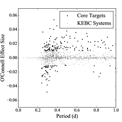
Figure 24: Plot comparing the OES to the period. Core sample targets are shown in black while non-target KEBC systems are shown in grey. The y-axis is in units of normalized flux. KICs 9777984, 9935311, and 11347875 are excluded for clarity. Note the positive correlation in core sample systems with $P<0.5$ d.

Figure 21’s top-left panel comparing OES and period shows that the OES tends towards zero at longer periods. This trend is consistent with the idea that binary interaction ultimately causes the O’Connell effect. The lack of any systems in our sample with a period greater than ten days strengthens this idea. Table 3 shows that this correlation is not robust. Of greater concern is that Table 3 indicates that the correlation between OES and period is positive in our sample, contradicting the trend observed in Figure 21. Our explanation for this contradiction is a positive trend between OES and period for the shortest period systems in our sample.

To better display this short-period system trend, Figure 24 shows a rescaled view of Figure 21’s top-left panel focusing on systems with periods under 1 d. Systems with $P\leq 0.5$ d show this positive correlation clearly. Since Figure 9 shows that most systems in our sample have $P\leq 0.5$ d, this positive correlation dominates the $\rho$ coefficient. We found that the $\rho$ coefficient for OES and period more than doubled ($\rho=0.425$) when analyzing only core sample systems with $P\leq 0.5$ d rather than the entire core sample, supporting our explanation. Furthermore, the short-period system correlation is robust (20 of 20 subsets show a correlation). When we analyzed the core sample systems with $P>0.5$ d, we found no correlation ($\rho=-0.069$). We interpret the short-period system trend as a result of the following: hotter systems ($T\geq 6,\!000$ K) almost always have OES $>0$ (as discussed in the previous paragraph), temperature is positively correlated with luminosity, and luminosity is positively correlated with orbital period (as discussed in Section 5.2.4). Therefore, the shortest period systems are more likely to have OES $<0$ than longer period systems, producing the observed trend.

Figure 25: Plots comparing the primary eclipse depth to $|$OES$|$. Core sample targets are shown in black while non-target KEBC systems are shown in grey. The red dashed line shows the ODR correlation for the KEBC. The left panel’s axes are scaled linearly, while the right panel’s axes are scaled logarithmically. Both axes are in units of normalized flux. KICs 9777984, 9935311, and 11347875 are excluded from the left panel for clarity. No correlation is apparent in the left panel, but a weak correlation can be seen in the right panel.

We expected strong correlations between $|$OES$|$ and other characteristics under the premise that the positive and negative O’Connell effects are fundamentally similar. This premise implies that the positive and negative OES correlations should strengthen when neglecting the OES’s sign. Therefore, we were surprised by the lack of such correlations in our core sample. The only $|$OES$|$ correlation we found was between $|$OES$|$ and the primary eclipse depth, and the correlation is both weak and not robust. Furthermore, Figure 25’s left panel shows no visible correlation between these two characteristics. The lack of $|$OES$|$ correlations implies that our premise that the positive and negative O’Connell effects are fundamentally similar is incorrect.

Note that every characteristic is correlated with $|$OES$|$ in the KEBC, the strongest of which is the correlation with primary eclipse depth. We determined a quadratic fit of $D=-298(19)|\text{OES}|^{2}+81(4)|\text{OES}|$ for this correlation using ODR, where $D$ is the primary eclipse depth and the parentheticals are the uncertainties. While we do not see this correlation in Figure 25’s left panel, either, Figure 25’s right panel showing a log-log plot of these characteristics displays a visible, if weak, correlation between them. We suspect that the $\rho$ coefficient detected this trend, resulting in the large coefficient in Table 3. Figure 25’s right panel indicates that this trend extends from our sample down to much smaller values of $|$OES$|$ and eclipse depth. Therefore, some systems that are not in our sample may be fundamentally similar to our sample’s systems, only with smaller values for $|$OES$|$ and eclipse depth. As such, this correlation may be more related to the O’Connell effect than its strength in our sample would indicate.

Both panels of Figure 25 also show a lack of systems displaying a significant O’Connell effect and a small primary eclipse depth. Our selection criterion ($|\text{OES}|\geq 0.01$) does not exclude such systems, and their absence is conspicuous since most KEBC systems have small eclipse depths. A bias in the Kepler selection function against these systems may explain their absence, which would imply a fundamental difference between such systems and the systems Kepler observed. Their absence may also be a true representation of O’Connell effect binaries, although we cannot identify a plausible reason why systems with a significant O’Connell effect cannot have a small primary eclipse depth. As a final note, Figure 25’s left panel shows that all four KEBC systems with an eclipse depth above 0.8 have a non-negligible $|$OES$|$.

We found different correlations for the OES (the morphology parameter, temperature, distance, absolute magnitude, and period) as compared to $|$OES$|$ (eclipse depth). Because the OES distinguishes between the positive and negative O’Connell effects but $|$OES$|$ does not, this suggests a more fundamental difference between the positive and negative O’Connell effects than previously thought. Assuming that spots are the O’Connell effect’s primary cause, a larger OES implies that spots cover a greater area, have a more extreme temperature factor, or are further offset from the line connecting the stellar centers. Kouzuma (2019) found a weak positive correlation between stellar temperature and spot temperature factor for cool starspots in W-type overcontact systems, wherein the smaller star is hotter (in contrast to A-type overcontact systems; McCartney 1999). The same correlation is much stronger in semi-detached systems. Kouzuma (2019) found weak positive correlations in overcontact systems between stellar temperature and spot size and between orbital period and spot size. The correlations for cool spots are similar but generally stronger than for hot spots. His results imply positive correlations between temperature and $|$OES$|$ and between orbital period and $|$OES$|$. Table 3 shows both correlations for OES but neither for $|$OES$|$.

To further test this correlation, we found the $\rho$ coefficient for the positive O’Connell effect systems and for the negative O’Connell effect systems. We found that the correlations for the positive O’Connell effect systems ($\rho_{\text{temp}}=0.122$ and $\rho_{\text{per}}=0.083$) are weak. Furthermore, while the correlations are much stronger for the negative O’Connell effect systems ($\rho_{\text{temp}}=0.402$ and $\rho_{\text{per}}=0.142$), the former has the wrong sign (i.e. the OES gets closer to zero as the temperature increases) while the latter is still weak. These correlations are therefore inconsistent with the results of Kouzuma2019 starspot study. However, such inconsistencies may not indicate that starspots do not cause the O’Connell effect. Instead, they may result from our sample’s mixture of systems with different O’Connell effect causes, or perhaps from differences between our sample and his. Determining the cause of these inconsistencies is beyond the scope of this paper.

The three other robust correlations that we have not discussed are between OES and the morphology parameter, distance, and absolute magnitude. We interpret these three correlations as arising from unrelated correlations with other characteristics. For instance, the correlation between the OES and absolute magnitude arises from the discussed correlation between OES and temperature combined with the strong correlation between temperature and absolute magnitude that is a well-known feature of main-sequence stars. We do not discuss these secondary correlations due to their dependence on other correlations that have a more fundamental explanation.

The different correlations we find among positive and negative O’Connell effect systems, combined with the fact that a much larger number of systems display a positive O’Connell effect, leads us to conclude that the preference for a brighter maximum following the primary eclipse is not an observational bias. It is instead fundamental to the O’Connell effect. Additionally, we conclude that the positive and negative O’Connell effects have different causes, or that one cause is common in one case and rare in the other. We consider these findings important results of our study.

5.2.2 Eclipse Depth

The primary eclipse depth (as defined in Section 3.1) is influenced by four parameters: temperature ratio, relative radii, component shapes, and orbital inclination. This section discusses the correlation between the eclipse depth and the morphology parameter. It also discusses a couple of trends between these two characteristics seen in Figure 22’s center panel.

The eclipse depth strongly correlates with the morphology parameter in our sample, while the KEBC shows a weaker correlation. We expect such a correlation because, as Wilson (2006) states, the eclipse depth is a monotonic function of the stellar radii ratio for overcontact systems (i.e. systems with a large morphology parameter). Meanwhile, Matijevič et al. (2012) notes that the primary eclipse width increases with the morphology parameter, and the eclipse widths measure the sum of the relative stellar radii. Thus, in overcontact systems, the primary eclipse depth decreases as the morphology parameter increases. The best fit to this correlation is the linear function $\mu=-2.13(13)D+1.26(9)$. The KEBC’s correlation is weaker as it includes more small $\mu$ systems, for which the eclipse depth and stellar radii ratio relation does not hold.

Figure 22’s center panel comparing the primary eclipse depth to the morphology parameter shows a sharp edge toward the panel’s right side in both our sample and the KEBC. This trend indicates that eclipses get shallower as $\mu$ increases above 0.7, a consequence of the relation discussed in the previous paragraph. The systems in our sample appear to be clustered along this edge in Figure 22’s center panel. This clustering indicates that O’Connell effect systems tend to have the deepest eclipses of systems with similar light curves (as measured by the morphology parameter), hinting at a connection between the OES and the eclipse depth. The clustering around the right edge is also seen with the non-core systems, although it is not as pronounced.

Figure 22’s center panel shows another trend: all KEBC systems with $D\geq 0.6$ have $\mu\approx 0.6$. Söderhjelm & Dischler (2005) states that the maximum eclipse depth for two main-sequence stars is 0.75 magnitudes (equivalent to a relative flux of 0.5), implying that systems with deeper eclipses must have an evolved component. Matijevič et al. (2012) says that a $\mu$ of 0.6 indicates a semi-detached system, which occurs when an evolving star fills its Roche lobe. This trend therefore make sense because close binaries with evolved components would be expected to have $\mu\approx 0.6$ by Matijevič et al. (2012). However, we cannot discount the possibility that this trend is a statistical artifact caused by the rarity of systems with such deep eclipses in the KEBC. Our eclipse depth determination method discussed in Section 3.1 may also influence this trend, as it can underestimate the eclipse depth of Algol-type systems.

5.2.3 Morphology Parameter

The morphology parameter (described in Section 3.3) is primarily a measure of eclipse widths (Matijevič et al., 2012), but it correlates well with the morphology class of a given system. We wish to reemphasize the point from Matijevič et al. (2012) that the morphology parameter only provides a “best-guess” estimate of the morphology class. This section focuses on the morphology parameter distribution shown in Figure 26. It also discusses the initially surprising correlation between the morphology parameter and temperature.

Figure 26: Histogram comparing the morphology parameters for 211 of the 212 core sample targets (solid red) and all 2,745 entries in the KEBC (dashed grey) that have $\mu\neq-1$. KIC 7667885 is not included because it lacks a value for $\mu$ (see discussion in Section 2.5). The two distributions differ significantly, particularly for $\mu<0.5$. The core sample also has few systems with $0.6\leq\mu\leq 0.7$.

Figure 26 shows a lower abundance of systems with $0.6\leq\mu\leq 0.7$. The same region is depleted in the KEBC, but not to the extent of our sample, suggesting that this underabundance is not wholly due to the parent population. Matijevič et al. (2012) states that systems with $\mu$ in this range are semi-detached. Our interpretation of systems in this range is that the accreting star grows larger with increasing morphology parameter, with the system becoming contact around $\mu=0.7$. The larger the accretor is, the less deeply a matter stream will penetrate into its potential well. The matter stream will therefore impact the surface with less energy and cause less dramatic heating. Assuming the accretor is on the main sequence, a larger star will be hotter, further reducing the degree of heating. These factors could cause the paucity of systems in this region of parameter space showing a significant O’Connell effect.

Figure 26 also shows that systems with $\mu\lesssim 0.5$ rarely show a significant O’Connell effect, and none with $\mu\leq 0.3$ do. This is significant because our selection criterion should not be biased with respect to $\mu$. Stars in systems with a small $\mu$ are generally farther apart and are less likely to significantly affect each other, so this result reinforces the link between binary interaction and the O’Connell effect discussed in Section 5.2.1.

We were surprised by the morphology parameter and temperature correlation because we assumed they would be uncorrelated. We now believe that this correlation results from a selection effect. Two processes work in tandem to cause this selection effect: the influence of geometry on the morphology parameter and the influence of the initial mass function (IMF) on temperature. Regarding the first process, eclipses only occur if $\Delta<R_{1}+R_{2}$ at $\phi=0$ (conjunction), where $\Delta=a\cos{i}$ (Prša, 2006, Equations 3.37 and 3.38) and the $R_{n}$ are the component radii. Therefore, closer binaries (smaller $a$) exhibit eclipses over a broader range of inclinations. Since the components of large morphology parameter systems are generally closer than in small morphology parameter systems, we are more likely to observe a given system eclipse in the former case. The IMF, meanwhile, makes hot stars rarer than cool stars, a fact compounded by Kepler’s selection biases discussed in Section 2.1. Acting together, these processes mean that most hot eclipsing binaries observed by Kepler should have large morphology parameters. The resulting dearth of hot, small morphology parameter systems creates an apparent positive correlation between the characteristics.

5.2.4 Period

The period is a function of component masses and orbital separation due to Kepler’s third law. This section discusses the correlation between the period and the absolute magnitude/luminosity in the core sample. Figure 23’s lower-left panel demonstrates this correlation in the dense clustering seen near the panel’s left side.

A correlation between period and absolute magnitude initially seems odd. Low luminosity stars can have very wide orbits, after all, while very luminous stars can be short-period contact binaries. However, there is a lower period limit for stars of a given luminosity. For example, on the main sequence, a star’s size and surface temperature (and thus absolute magnitude) are a function of its mass. If binary components are too close, however, they will merge into a single star. Kepler’s third law states that $P\propto a^{1/3}$, while the Stefan-Boltzmann law states that $L_{*}\propto R^{2}$. Therefore, a lower limit on component separation based on stellar radius implies a lower limit on the period for a given absolute magnitude for main-sequence stars. This limit increases for evolved stars since they become cooler and larger as they evolve. The correlation between period and absolute magnitude is weaker in the KEBC because of the KEBC’s numerous long-period systems, which do not have a relationship between component separation and stellar radius.

Figure 27: Plot comparing the luminosity to the period. Core sample targets are shown in black while non-target KEBC systems are shown in grey. KICs 3662635 and 5820209 are excluded for clarity. The sharp edge near the lower-left corner denotes the short-period limit for a given luminosity. Most of the core sample is clustered near or along this edge.

Both Figure 23’s lower-left panel and Figure 27 show a tight clustering of systems along their left edge. Our interpretation of this clustering is that it represents the lower limit on the period for a given absolute magnitude or luminosity. Systems to the left of this edge are likely subdwarf systems or have poorly determined distances resulting in large luminosity errors. The fact that such a large percentage of our sample lies on or near this edge – particularly systems with $L_{*}\geq 1~{}\text{L}_{\odot}$ in Figure 27 – suggests that the O’Connell effect is more common in contact or near-contact binaries. This trend is therefore strong evidence that binary interaction is a critical factor in causing the O’Connell effect.

6 Conclusion

Our study of the characteristics of systems displaying a significant O’Connell effect takes advantage of the unprecedented amount of data available from the Kepler and Gaia missions. It represents a significant step forward in our understanding of this poorly understood phenomenon. We studied a significantly different parameter space than the earlier works of O51 and D84 out of necessity: we lack detailed information on the bulk characteristics of the component stars that were the basis of those works. We instead focused on those observational properties we could directly determine from the data currently available.

We found a significant O’Connell effect in 212 eclipsing binaries, with the 211 KEBC systems representing 7.3% of the 2,907 systems cataloged in the KEBC. This shows that a significant O’Connell effect is present in a non-negligible fraction of eclipsing binaries. Our core sample systems range in period from a quarter of a day to nearly ten days, temperature from around 3,800 K to 8,500 K, and luminosity from two-hundredths of a solar luminosity to over fifty solar luminosities. Clearly, a wide range of system types shows this phenomenon.

The O’Connell effect also manifests itself quite differently in different systems. Many systems have light curves that vary wildly with time, and the O’Connell effect varies along with it. Other systems have extremely stable light curves and a stable value of the OES. The existence of the latter type of system would indicate a cause of the O’Connell effect that is more stable in time than starspots, such as a hotspot caused by mass transfer. Furthermore, up to 20% of our sample displays the ETV signal associated with mass transfer. We conclude that there are multiple causes of the O’Connell effect.

The dearth of hot ($T\geq 6,\!000$ K) systems displaying a negative O’Connell effect is a new result and can be interpreted as evidence that starspots cause the O’Connell effect in negative O’Connell effect systems. Additionally, we found a moderate correlation between OES and temperature and a weaker correlation between OES and period, both predicted by Kouzuma2019 study on starspots, which also suggests that starspots predominately cause the O’Connell effect. However, looking at positive and negative O’Connell effects separately does not yield the same correlations. Instead, we found correlations that are inconsistent with Kouzuma2019 results. Therefore, we draw no conclusion as to whether starspots are a predominant cause of the O’Connell effect, but note that the idea is plausible. At the same time, it should not automatically be assumed that starspots cause the O’Connell effect in a given system without further supporting evidence for starspots. Many more systems display a positive O’Connell effect than a negative one, suggesting that which maximum is brighter is not chance but fundamentally tied to the O’Connell effect. We conclude that, whatever the physical causes of the O’Connell effect are, they preferentially cause the maximum following the primary eclipse to be brighter than the one preceding it.

The overarching trend found in this study is that the O’Connell effect and binary interaction are strongly correlated. We do not see this phenomenon in binaries with widely separated stars, and we almost always see evidence (ellipticity effects in light curves) of non-spherical stars in our sample. Looking beyond our sample, W Crucis (Zoła, 1996; Pavlovski et al., 2006) exhibits the O’Connell effect, and its light curve indicates an interacting, semi-detached system similar to other systems in our sample. However, W Crucis’ 198-day orbital period – the longest of an O’Connell effect binary that we are aware of – is over 20 times longer than the longest period in our sample. Nevertheless, W Crucis’ ellipsoidal variations shows that it has interacting components despite the long period, reinforcing the correlation between binary interaction and the O’Connell effect. We conclude that this correlation and the physical causes of the O’Connell effect are related: the interaction (whether gravitational, magnetic, or physical) between close binary stars causes the O’Connell effect instead of a phenomenon an isolated star (including non-interacting components in wider binaries) would display. If the phenomenon occurred on isolated stars, we would expect to see the O’Connell effect in all types of binaries, not just those with interacting components.

There are several ways to expand upon our work in the future. The recently published TESS Eclipsing Binary Catalog (TEBC; Prša et al., 2022) provides an opportunity to expand our analysis to a much larger data set. Gaia Data Release 3 (DR3) – currently slated for release in 2022 – will include Gaia time-series photometry for eclipsing binaries (Gaia Collaboration et al., 2019). Gaia’s tricolor photometry allows temperature measurements for both stars and an exploration of the O’Connell effect’s temperature dependence. This data greatly increases the parameter space available for study. We will further discuss the system classes Section 4.5 described in future work. This discussion will include searching for periodicities and quasi-periodicities in temporally varying systems, finding the second and third derivatives of concave-up systems to quantify their properties, and determining the degree of asymmetry in asymmetric minima systems. We will also discuss the subset of our sample brighter than $K_{p}=14$ in future work due to Wolniewicz et al. (2021) finding such systems to be unbiased. The new Kepler eclipsing binaries Bienias et al. (2021) found require further study to ensure our sample’s completeness. Future work will also discuss our observations of ten sample systems and the PHOEBE (Prša & Zwitter, 2005; Prša et al., 2016) models we create using our data. Analysis of the sub-groupings seen in Figures 21-23 is left for a future study. Finally, we intend to further study the differences between the positive and negative O’Connell effects our study found.

Table 1: Complete Kepler O’Connell Effect Target List

Kepler	R.A. (J2000)	Dec. (J2000)	Period	LC	Morph.	BP – RP	Gaia	Gaia	Dist.	Lum.	Spectral Type		Ref.	Samp.	Notes
ID	hh:mm:ss.s	+dd:mm:ss.ss	(days)	Class	Param.	Color	BP Mag.	G Mag.	(pc)	(L⊙)	Lit.	Color
2159783	19:25:26.2	+37:33:11.90	0.3739	WU	0.87	0.938	15.365	14.982	1546	1.810	F6 V1	G9	4, 5, 6, 22*	C	AM, S, M
2161623	19:26:58.7	+37:35:27.60	2.2835	Al	0.54	0.771	14.571	14.273	1901	5.262	$\cdots$	F9.5	$\cdots$	C	$\cdots$
2302092	19:25:02.9	+37:41:52.49	0.2947	WU	0.88	1.124	14.982	14.503	811	0.775	$\cdots$	K2	5, 7	C	S
2305372	19:27:57.7	+37:40:21.83	1.4047	Al	0.58	0.929	14.214	13.846	1273	3.498	F8 Vs1	G9	2, 7, 13, 14*, 16, 19	C	F
2437038	19:20:47.6	+37:44:31.83	0.2677	WU	0.87	1.120	16.501	16.149	2784	2.004	$\cdots$	K2	3, 5, 6	C	F, S, M
2449084	19:30:46.9	+37:46:19.13	0.7398	BL	0.70	0.842	15.319	14.983	2798	5.926	$\cdots$	G4	3	C	AM, F
2569494	19:20:42.9	+37:50:56.26	1.5233	Al	0.58	1.209	17.799	17.288	4760	2.051	$\cdots$	K3	8, 13	C	TV, AM
2577756	19:27:26.9	+37:49:47.77	0.8703	Al	0.63	0.911	15.860	15.491	2185	2.262	$\cdots$	G8	2	M	TV, AM, F
2694741	19:05:39.0	+37:54:29.65	0.3266	WU	0.93	0.936	12.639	12.256	373	1.304	G4 V1	G9	3, 5	C	F, S
2695740	19:06:55.4	+37:56:39.53	3.6159	WU	0.85	1.305	13.704	13.126	1453	8.844	$\cdots$	K4	3, 5, 19	C	TV, AM, F, S
2854752	19:27:44.6	+38:00:22.65	0.4704	BL	0.79	0.636	14.153	13.918	1594	5.132	$\cdots$	F6	3, 6	C	F, M
2858322	19:30:41.9	+38:03:53.38	0.4364	BL	0.77	0.984	15.197	14.789	2133	4.118	$\cdots$	K0	5, 6	C	S, M
2972514	19:06:44.6	+38:10:12.89	0.5035	WU	0.74	0.802	14.332	14.020	1361	3.405	$\cdots$	G1	$\cdots$	C	$\cdots$
3124420	19:32:58.9	+38:16:18.68	0.9490	Al	0.60	1.174	18.801	18.287	5120	0.946	$\cdots$	K2.5	$\cdots$	C	TV, AM
3218683	19:05:36.1	+38:22:34.22	0.7717	Al	0.69	1.156	16.524	16.030	2046	1.208	$\cdots$	K2.5	2, 5	C	F, S
3338660	19:21:53.8	+38:25:38.62	1.8734	Al	0.60	0.944	15.087	14.707	3515	12.053	$\cdots$	G9	3, 7, 8	C	F
3339563	19:22:59.0	+38:26:35.33	0.8412	BL	0.72	1.030	14.624	14.193	1195	2.240	G0 IIIp1	K1	2, 3, 5	C	TV, AM, F, S
3342425	19:26:03.9	+38:27:16.06	0.3934	WU	0.94	0.898	15.489	15.137	1896	2.362	$\cdots$	G8	3, 5	C	TV, AM, F, S
3344427	19:28:00.6	+38:26:06.69	0.6518	Al	0.57	1.448	16.423	15.776	866	0.274	$\cdots$	K5	$\cdots$	M	$\cdots$
3351945	19:35:32.3	+38:26:44.56	1.0805	Al	0.50	1.288	15.359	14.794	483	0.210	$\cdots$	K3.5	$\cdots$	M	TV
3557421	19:38:32.4	+38:37:36.86	0.3937	Al	0.70	1.124	10.486	10.003	94	0.662	$\cdots$	K2	5, 16, 19	M	S
3656322	19:36:38.5	+38:46:02.73	3.6637	Al	0.59	1.125	13.538	13.077	1036	4.706	$\cdots$	K2	13	M	TV
3659940	19:40:01.1	+38:46:31.65	0.8963	Al	0.55	1.047	15.619	15.187	1197	0.899	$\cdots$	K1.5	$\cdots$	C	TV
3662635	19:42:16.6	+38:43:33.81	0.9394	Al	0.57	0.988	15.273	14.965	6474	32.241	$\cdots$	K0	3	C	TV, F
3743834	19:22:11.1	+38:52:21.35	0.2736	WU	0.76	1.218	14.775	14.241	517	0.402	$\cdots$	K3	3, 5	C	F, S
3832382	19:00:59.1	+38:58:59.86	0.2726	WU	0.75	1.426	16.447	15.802	918	0.300	$\cdots$	K5	5	C	S
3839964	19:13:10.5	+38:58:41.03	0.2561	WU	0.80	1.026	14.988	14.557	1065	1.272	$\cdots$	K1	3, 7	M	F
3848919	19:24:13.5	+38:58:27.83	1.0473	Al	0.57	1.059	14.409	13.984	817	1.269	$\cdots$	K1.5	21	C	$\cdots$
3954227	19:25:58.3	+39:03:00.51	0.5943	Al	0.56	1.434	16.689	16.097	1151	0.359	$\cdots$	K5	$\cdots$	M	TV
3965242	19:37:17.1	+39:02:20.00	0.9967	Al	0.53	1.074	14.536	14.084	478	0.396	$\cdots$	K1.5	$\cdots$	C	TV
3972629	19:43:43.9	+39:01:29.58	0.2442	BL	0.85	1.140	15.448	14.957	720	0.403	$\cdots$	K2.5	3, 5	C	F, S
4037163	19:00:19.2	+39:11:02.44	0.6354	Al	0.59	1.484	18.153	17.446	2139	0.358	$\cdots$	K5.5	7, 8	M	TV
4049124	19:17:15.4	+39:07:52.90	4.8045	Al	0.17	1.007	15.063	14.647	934	0.900	$\cdots$	K1	2, 13	M	F
4077442	19:45:21.9	+39:08:26.06	0.6928	Al	0.59	1.325	14.213	13.629	545	0.785	$\cdots$	K4	21	M	TV
4168013	19:36:10.5	+39:15:59.55	0.3109	WU	0.85	1.092	15.527	15.079	1124	0.875	$\cdots$	K2	$\cdots$	M	$\cdots$
4241946	18:59:36.6	+39:20:50.52	0.2844	WU	0.75	1.329	16.472	16.073	5779	9.260	$\cdots$	K4	3	C	F
4249218	19:10:49.9	+39:18:48.69	0.3162	WU	0.76	1.053	14.449	14.184	801	1.015	G4 V1	K1.5	3, 5, 19	C	F, S
4349483	19:06:35.4	+39:27:17.00	0.5091	Al	0.71	1.243	14.798	14.371	641	0.546	$\cdots$	K3.5	$\cdots$	C	TV
4350454	19:08:12.6	+39:29:16.53	0.9657	BL	0.80	0.829	13.934	13.608	1861	9.305	$\cdots$	G3	3	C	F
4385109	19:45:02.2	+39:25:17.15	0.2746	WU	0.90	1.181	15.580	15.071	875	0.535	$\cdots$	K2.5	3	C	F
4466691	19:29:07.0	+39:30:18.22	0.4827	BL	0.78	0.688	14.576	14.308	2027	5.792	$\cdots$	F8	$\cdots$	C	$\cdots$
4474193	19:36:57.5	+39:33:30.45	0.3225	WU	0.89	1.067	15.628	15.173	1268	1.022	$\cdots$	K1.5	3, 5	C	TV, F, S
4474637	19:37:21.6	+39:33:47.85	3.8867	Al	0.58	0.911	18.111	17.780	7742	3.450	$\cdots$	G8	13	C	TV, AM
4547308	19:08:14.6	+39:39:54.54	0.5769	WU	0.88	0.552	12.617	12.457	1654	21.215	$\cdots$	F4	3, 7	C	F
4660997	19:34:03.3	+39:42:41.00	0.5626	Al	0.62	0.885	12.606	12.250	431	1.742	G1 V1	G7	1, 3, 14, 16, 17, 19, 21	M	F
4859432	19:50:13.1	+39:59:00.27	0.3855	WU	0.77	1.064	15.651	15.214	1702	1.773	$\cdots$	K1.5	3, 7	C	F
4941060	19:44:39.7	+40:04:47.95	0.3034	WU	0.75	1.160	15.892	15.403	1105	0.628	$\cdots$	K2.5	5	C	S
4991959	18:59:13.7	+40:09:20.95	0.3609	WU	0.76	0.943	15.442	15.053	1353	1.300	$\cdots$	G9	3, 5, 6	C	F, S, M
5020034	19:37:12.9	+40:11:33.18	2.1191	Al	0.57	0.884	16.110	15.761	4511	7.522	$\cdots$	G7	$\cdots$	C	$\cdots$
5033682	19:48:57.3	+40:10:15.60	0.3799	WU	0.94	0.892	13.640	13.278	741	2.000	$\cdots$	G8	3, 4, 5	C	F, S
5123176	19:50:33.6	+40:14:09.90	0.7078	WU	0.82	0.622	11.713	11.481	765	11.153	F5 IV1	F6	3, 5, 6, 16, 17, 19	C	F, S, M
5195137	19:36:25.2	+40:18:05.89	0.3241	WU	0.92	1.007	14.426	14.010	770	1.099	$\cdots$	K1	3, 5	C	F, S
5215999	19:54:19.8	+40:21:53.07	2.5312	Al	0.68	1.134	14.636	14.155	3216	16.783	$\cdots$	K2	3, 5	M	TV, F, S
5282464	19:35:47.0	+40:26:58.34	0.4964	BL	0.73	0.491	12.708	12.524	918	6.144	$\cdots$	F2	16, 19	C	$\cdots$
5283839	19:37:12.7	+40:28:00.66	0.3152	WU	0.93	0.892	15.614	15.253	1587	1.486	$\cdots$	G8	3, 4, 5	M	AM, F, S
5294739	19:47:20.9	+40:28:23.16	3.7360	Al	0.59	1.255	14.111	13.567	1688	7.949	$\cdots$	K3.5	3, 13, 16, 19	C	F
5300878	19:52:19.6	+40:28:41.29	1.2794	Al	0.50	1.387	15.583	14.963	626	0.303	$\cdots$	K4.5	5, 8	C	CU, S
5357682	19:21:13.2	+40:34:12.02	0.7177	BL	0.83	0.741	14.801	14.511	2118	5.242	$\cdots$	F9	$\cdots$	C	$\cdots$
5425950	18:52:13.7	+40:41:17.55	0.3782	WU	0.76	0.979	15.534	15.136	1418	1.323	$\cdots$	K0	5	C	S
5543482	19:38:34.2	+40:43:47.36	0.2948	WU	0.80	1.154	16.171	15.680	1294	0.667	$\cdots$	K2.5	$\cdots$	C	$\cdots$
5557368	19:50:56.4	+40:46:04.24	0.2979	WU	0.93	1.086	13.220	12.756	360	0.765	$\cdots$	K2	3, 5, 16, 19	C	F, S
5563814	19:56:16.1	+40:43:15.45	0.3082	WU	0.91	1.135	15.634	15.184	1259	0.997	$\cdots$	K2	3, 5	C	F, S
5615528	19:21:38.1	+40:49:43.27	0.3392	Al	0.70	0.852	14.912	14.672	1304	1.714	$\cdots$	G5	$\cdots$	M	TV
5774375	19:03:42.2	+41:05:26.93	1.5500	Al	0.60	1.092	14.375	13.915	1334	3.604	$\cdots$	K2	2, 3	C	TV, F
5820209	19:55:57.7	+41:03:52.27	0.6561	BL	0.81	1.310	14.095	13.519	4153	50.251	$\cdots$	K4	6, 11	C	M
5956588	19:22:20.2	+41:14:06.72	0.2729	WU	0.83	1.083	16.217	15.755	1296	0.625	$\cdots$	K2	$\cdots$	C	$\cdots$
5984000	19:51:32.3	+41:14:57.97	0.3231	WU	0.82	0.998	14.845	14.435	925	1.074	$\cdots$	K0.5	3, 5	C	F, S
6034812	19:17:20.8	+41:19:06.82	0.3673	WU	0.93	0.765	13.143	12.844	696	2.633	F51	F9.5	3	M	TV, F
6044064	19:29:24.8	+41:19:27.26	5.0632	Al	0.54	1.070	15.527	15.081	2981	6.145	$\cdots$	K1.5	2, 3, 13, 23*	C	CU, F
6050116	19:36:33.1	+41:20:22.56	0.2399	WU	0.79	1.280	14.948	14.392	448	0.262	$\cdots$	K3.5	3, 5, 19†, 24*	C	F, S
6103049	18:55:04.4	+41:26:27.97	0.6432	Al	0.59	0.931	15.462	15.083	2358	3.839	$\cdots$	G9	2, 7	M	F
6106771	19:02:18.9	+41:26:15.94	0.2638	WU	0.77	1.032	16.041	15.598	1136	0.554	$\cdots$	K1.5	3	C	F
6128248	19:33:07.4	+41:26:08.39	0.2917	WU	0.76	1.238	15.808	15.267	850	0.421	$\cdots$	K3	5	C	S
6191574	19:08:42.5	+41:31:59.23	1.0345	Al	0.50	1.560	15.013	14.310	271	0.103	$\cdots$	K6	2	M	TV, F
6197038	19:17:12.2	+41:31:35.40	9.7517	Al	0.46	1.224	13.919	13.381	1468	7.136	$\cdots$	K3	2	C	TV, CU, F
6205460	19:27:55.3	+41:33:33.90	3.7228	Al	0.58	1.065	12.957	12.558	778	4.282	$\cdots$	K1.5	1, 2, 3, 13, 16, 19	C	AM, F
6223646	19:47:32.0	+41:31:07.90	0.3649	WU	0.84	0.474	13.655	13.482	1235	4.600	B9 III1	F2	19	C	$\cdots$
6264091	18:52:59.6	+41:39:11.22	0.3250	WU	0.97	0.936	15.524	15.144	1607	1.685	$\cdots$	G9	3, 5	C	TV, F, S
6267702	19:00:00.8	+41:38:29.04	0.2832	BL	0.90	1.128	16.021	15.783	1137	0.469	$\cdots$	K2	3	M	TV, F
6283224	19:24:46.0	+41:40:01.94	0.7665	Al	0.57	1.128	16.021	15.541	1350	0.825	$\cdots$	K2	2	M	F
6421483	18:52:10.8	+41:51:36.26	2.1584	Al	0.58	1.119	13.595	13.120	757	2.415	$\cdots$	K2	3	C	TV, AM, F
6424124	18:57:21.9	+41:50:19.32	0.3855	WU	0.91	0.872	14.275	13.920	1021	2.102	F7 III1	G6	3, 5, 6, 19	C	F, S, M
6431545	19:11:18.9	+41:48:17.79	0.3168	WU	0.91	0.963	14.146	13.751	723	1.230	G2 V1	G9	3, 5*, 7*‡	M	TV, F, S
6436038	19:18:10.1	+41:53:25.24	0.3763	WU	0.96	0.917	15.588	15.219	1789	1.949	$\cdots$	G8	3	C	TV, F
6471048	19:56:30.8	+41:49:41.89	0.2972	WU	0.77	1.159	13.287	12.784	309	0.549	K0 V1	K2.5	5, 19	C	S
6615041	19:37:26.9	+42:02:45.31	0.3401	WU	0.76	0.877	14.056	13.713	731	1.304	Flat1	G7	5, 7, 19	C	S
6697716	19:34:22.7	+42:08:35.19	1.4432	Al	0.44	1.172	14.918	14.417	806	0.828	$\cdots$	K2.5	$\cdots$	M	CU
6791604	19:42:42.1	+42:14:26.14	0.5288	BL	0.70	0.555	14.098	13.896	1615	5.373	$\cdots$	F4	6	C	M
6836140	18:44:09.8	+42:23:52.30	0.4877	WU	0.73	1.139	15.215	14.737	1000	0.950	$\cdots$	K2.5	1, 3, 5	C	TV, F, S
6962018	19:42:10.5	+42:25:42.24	1.2699	Al	0.45	1.657	15.577	14.785	380	0.132	$\cdots$	K6.5	$\cdots$	C	$\cdots$
7035139	19:29:08.1	+42:35:40.46	0.3097	WU	0.80	1.011	15.950	15.543	1372	0.851	$\cdots$	K1	5	M	S
7037319	19:31:47.6	+42:30:30.38	0.5781	BL	0.84	0.592	13.808	13.587	1850	9.375	$\cdots$	F5	3	C	F
7119757	19:29:35.6	+42:37:47.63	0.7429	Al	0.64	1.134	16.118	15.636	2106	1.839	$\cdots$	K2	2, 3, 5, 7	M	TV, F, S
7173910	18:44:48.7	+42:44:45.86	0.4022	WU	0.82	0.878	14.719	14.360	1298	2.263	$\cdots$	G7	5	M	S
7199183	19:25:43.0	+42:47:10.56	0.3241	WU	0.97	1.003	16.086	15.667	1584	1.012	$\cdots$	K0.5	3	C	TV, F
7199353	19:25:56.4	+42:44:15.93	0.2820	WU	0.78	1.054	14.953	14.530	736	0.623	$\cdots$	K1.5	3, 5	C	F, S
7259917	18:53:02.2	+42:50:44.15	0.3847	BL	0.70	0.711	12.132	11.867	412	2.267	F3 V1	F9	5, 17, 19	C	S
7272739	19:15:25.7	+42:48:45.21	0.2812	WU	0.77	1.060	13.445	12.982	350	0.588	$\cdots$	K1.5	3, 5, 7, 17, 19†	C	F, S
7284688	19:30:31.2	+42:49:45.63	0.6460	Al	0.64	0.942	11.918	11.930	$\cdots$	$\cdots$	G2 V1	G9	2, 5, 9	M	TV, F, S
7367833	19:33:20.4	+42:55:18.87	0.2862	Al	0.77	0.940	15.793	15.412	1912	1.864	$\cdots$	G9	$\cdots$	M	$\cdots$
7433513	19:12:27.9	+43:05:39.41	0.7011	Al	0.70	0.966	15.872	15.482	1661	1.319	$\cdots$	K0	$\cdots$	C	TV, AM
7458285	19:42:10.3	+43:02:56.97	0.6606	BL	0.71	0.813	13.848	13.527	1462	6.189	F0 IV1	G1	6	C	M
7516345	19:12:15.0	+43:07:39.28	0.4919	BL	0.75	0.506	12.499	12.311	873	6.761	$\cdots$	F3	5, 19†	C	S
7542091	19:42:52.0	+43:09:52.62	0.3905	WU	0.83	0.860	12.711	12.369	490	2.021	G1 V1	G6	3, 4, 5, 17, 19	C	F, S
7546429	19:46:46.9	+43:08:18.82	0.3521	WU	0.92	0.998	15.608	15.196	1580	1.553	$\cdots$	K0.5	$\cdots$	C	$\cdots$
7584739	18:49:09.9	+43:17:02.16	0.9116	BL	0.72	0.651	13.691	13.452	1860	10.721	F3 V1	F6	3, 6, 17†, 19†	C	F, M
7584826	18:49:23.1	+43:17:04.20	0.6223	Al	0.62	0.992	15.654	15.255	1337	1.053	$\cdots$	K0.5	5	C	TV, S
7610486	19:30:55.6	+43:14:41.50	0.4577	WU	0.80	0.940	16.107	15.788	2400	2.076	$\cdots$	G9	5	C	S
7627059	19:48:27.4	+43:12:51.59	0.3237	WU	0.81	0.957	15.362	14.976	1310	1.308	$\cdots$	G9	3	C	F
7657914	18:39:52.3	+43:23:08.43	0.4745	BL	0.72	0.581	13.178	12.979	951	4.336	F5 Vaw1	F5	17, 19	C	$\cdots$
7667885	19:03:30.3	+43:23:22.47	0.3148	Al	$\cdots$	1.413	17.450	16.827	1374	0.262	G2	K4.5	3, 20*	C	F
7671594	19:10:32.6	+43:22:14.95	1.4103	Al	0.34	2.369	16.980	15.719	209	0.017	$\cdots$	M2.5	2, 13	C	TV, CU, F
7685689	19:31:30.5	+43:22:07.25	0.3252	WU	0.78	0.955	15.955	15.579	1587	1.101	$\cdots$	G9	7	C	$\cdots$
7696778	19:45:09.1	+43:23:55.39	0.3312	WU	0.79	1.209	15.931	15.409	1331	0.906	$\cdots$	K3	$\cdots$	C	$\cdots$
7740566	19:07:08.0	+43:25:50.82	0.2971	WU	0.81	0.951	16.030	15.696	1611	1.019	$\cdots$	G9	3	C	F
7773380	19:51:27.4	+43:29:52.71	0.3076	WU	0.94	1.041	14.863	14.434	859	0.927	$\cdots$	K1.5	3, 4, 5	C	F, S
7871200	18:50:52.4	+43:40:12.05	0.2429	WU	0.75	1.335	13.614	13.030	262	0.315	$\cdots$	K4	3, 6, 17, 19, 25*	C	F, M
7877062	19:03:35.7	+43:36:12.29	0.3037	WU	0.82	0.943	14.285	13.898	682	0.956	$\cdots$	G9	3, 5, 7, 19	C	F, S
7879399	19:08:29.9	+43:36:00.64	0.3927	WU	0.74	0.900	12.980	12.599	506	1.744	$\cdots$	G8	19†	C	$\cdots$
7885570	19:19:53.7	+43:39:13.77	1.7293	Al	0.58	0.890	12.046	11.686	510	4.115	G0 IV1	G7	1, 2, 3, 19, 26*	M	TV, AM:SC, F
7950962	19:13:38.5	+43:42:26.77	0.8270	WU	0.94	0.524	10.794	10.621	644	17.477	$\cdots$	F3	3, 19	C	F
7959612	19:26:37.0	+43:44:13.63	0.2432	WU	0.81	1.297	17.513	16.947	1444	0.258	$\cdots$	K4	$\cdots$	C	$\cdots$
8029708	19:28:37.6	+43:49:06.96	0.3136	BL	0.75	1.165	17.215	16.731	1816	0.499	$\cdots$	K2.5	$\cdots$	C	$\cdots$
8112324	19:46:35.4	+43:59:41.99	0.5759	Al	0.59	1.086	15.126	14.675	920	0.850	$\cdots$	K2	$\cdots$	C	TV
8190491	19:56:21.6	+44:04:01.45	0.7779	BL	0.95	0.826	14.554	14.226	2705	11.116	$\cdots$	G2	5, 7	C	S
8211618	18:46:26.9	+44:07:34.64	0.3374	WU	0.74	0.969	16.068	15.667	1668	1.121	$\cdots$	K0	$\cdots$	C	$\cdots$
8211824	18:46:58.7	+44:10:10.75	0.8411	Al	0.59	1.215	16.600	16.075	1315	0.479	$\cdots$	K3	2	C	TV, F
8230815	19:23:34.4	+44:07:52.49	0.3452	WU	0.93	0.854	13.640	13.298	683	1.666	G0.5 V1	G5	3, 5	C	F, S
8248967	19:47:46.6	+44:09:59.05	0.5925	WU	0.83	0.799	15.439	15.112	3218	6.960	$\cdots$	G1	$\cdots$	C	AM
8285349	19:02:27.9	+44:12:56.42	0.6671	BL	0.90	0.712	12.437	12.166	570	3.293	F3/F5 V1	F9	2, 3, 5, 18	M	TV, F, S
8294484	19:19:45.7	+44:13:32.55	1.0127	Al	0.58	0.832	15.152	14.827	1611	2.269	$\cdots$	G3	$\cdots$	C	TV, AM
8298344	19:25:08.6	+44:12:57.21	0.3029	WU	0.93	1.120	15.780	15.305	1100	0.681	$\cdots$	K2	3, 5	C	TV, F, S
8386048	19:52:51.9	+44:19:25.43	0.8174	BL	0.71	1.031	17.059	16.631	5100	4.314	$\cdots$	K1.5	3	C	F
8431389	19:28:12.2	+44:28:25.71	0.3511	WU	0.84	0.938	15.058	14.689	1337	1.774	$\cdots$	G9	6	C	M
8479107	18:56:30.1	+44:33:01.98	0.7676	Al	0.53	1.087	15.464	15.010	887	0.582	$\cdots$	K2	2, 5	M	TV, F, S
8608490	18:56:40.1	+44:46:45.74	1.0828	Al	0.51	1.125	15.427	14.955	851	0.563	$\cdots$	K2	1, 3, 5	C	F, S
8620561	19:21:04.1	+44:42:41.21	0.7820	Al	0.53	1.408	17.439	16.808	1259	0.223	$\cdots$	K4.5	$\cdots$	C	$\cdots$
8690104	19:28:37.9	+44:52:24.35	0.4088	WU	0.77	0.872	15.261	14.913	1572	1.994	$\cdots$	G6	5, 6, 7	C	S, M
8694926	19:36:08.7	+44:49:46.34	0.3715	WU	0.80	0.995	16.050	15.693	4386	7.570	$\cdots$	K0.5	$\cdots$	M	$\cdots$
8696327	19:38:02.7	+44:48:24.22	0.8792	BL	0.75	0.708	14.850	14.575	2923	9.412	$\cdots$	F9	$\cdots$	C	AM
8703528	19:47:18.8	+44:48:07.59	0.3999	WU	0.75	0.990	13.411	12.992	555	1.462	$\cdots$	K0	3, 6, 17, 19†	C	F, M
8715667	20:00:06.5	+44:49:05.02	0.4057	WU	0.85	1.034	13.873	13.516	1124	3.695	$\cdots$	K1.5	3, 5, 19†	C	F, S
8822555	19:33:10.4	+45:02:31.20	0.8528	BL	0.80	0.742	14.570	14.282	2501	9.029	$\cdots$	F9	$\cdots$	C	AM
8842170	19:57:14.5	+45:03:48.88	0.3494	WU	0.90	1.025	15.200	14.771	1318	1.598	$\cdots$	K1	10	C	AM
8846978	20:02:43.3	+45:00:07.76	1.3791	Al	0.77	1.098	13.716	13.254	887	2.929	$\cdots$	K2	3, 5, 11	C	TV, F, S
8904448	19:51:31.6	+45:07:34.94	0.8660	BL	0.74	0.516	14.008	13.814	2734	16.603	A2 V1	F3	3, 7, 19	C	F
8934111	18:53:23.9	+45:17:50.46	0.3645	WU	0.92	0.943	15.553	15.169	1632	1.699	$\cdots$	G9	3, 5	C	F, S
8949316	19:22:04.6	+45:14:07.36	0.6044	Al	0.51	2.247	17.317	16.148	423	0.046	$\cdots$	M2	8	M	$\cdots$
8977390	19:55:44.2	+45:17:51.59	0.6533	WU	0.86	0.781	13.427	13.125	1399	8.199	F0 IV1	G0	3, 19	C	F
9071104	18:51:56.6	+45:24:28.73	0.3852	WU	0.82	0.820	13.958	13.627	923	2.249	$\cdots$	G2	4, 5, 18, 19	C	S
9071373	18:52:38.2	+45:24:56.24	0.4218	BL	0.81	0.836	13.313	12.974	753	2.733	G0 V1	G3	3, 5, 18	C	F, S
9091810	19:31:48.0	+45:25:11.88	0.4797	Al	0.70	0.970	13.006	12.601	457	1.418	$\cdots$	K0	1, 3, 5, 7, 11	C	F, S
9101279	19:44:00.4	+45:26:53.24	1.8115	Al	0.58	0.535	13.916	13.721	2116	10.832	$\cdots$	F4	7*, 13	C	$\cdots$
9119652	20:03:49.7	+45:26:57.13	2.2162	Al	0.43	1.156	14.821	14.327	790	0.864	$\cdots$	K2.5	13	C	CU
9137992	18:53:50.5	+45:33:20.95	1.4700	Al	0.64	0.936	13.388	13.004	862	3.479	G5.5 IIb1	G9	3, 18	C	TV, F
9145707	19:10:59.4	+45:31:04.94	0.3208	WU	0.75	0.993	15.152	14.740	990	0.927	$\cdots$	K0.5	3, 5, 6, 18	C	F, S, M
9145846	19:11:19.8	+45:35:24.98	0.2945	WU	0.96	1.246	15.818	15.276	559	0.181	$\cdots$	K3.5	3, 5	C	TV, F, S
9161428	19:37:42.0	+45:30:21.51	0.3026	WU	0.92	0.967	15.515	15.123	1256	1.049	$\cdots$	K0	3	C	F
9164694	19:42:39.8	+45:30:24.70	1.1114	BL	0.75	0.744	14.386	14.107	2674	12.125	$\cdots$	F9.5	3, 15*	C	AM, F
9274472	19:15:58.7	+45:46:44.84	0.3021	WU	0.90	1.103	14.420	13.948	595	0.697	$\cdots$	K2	3, 5, 18	C	F, S
9283826	19:32:10.9	+45:44:08.92	0.3565	WU	0.84	0.854	13.460	13.124	645	1.749	$\cdots$	G5	3, 5, 6, 7, 19	C	AM, F, S, M
9290838	19:42:36.0	+45:47:02.22	0.3630	WU	0.92	1.011	15.890	15.489	1718	1.402	$\cdots$	K1	3, 5	C	F, S
9307423	20:02:22.1	+45:45:26.92	0.5586	WU	0.73	1.402	16.762	16.150	1933	0.965	$\cdots$	K4.5	$\cdots$	C	$\cdots$
9328852	18:59:59.3	+45:53:12.08	0.6459	Al	0.54	1.402	15.919	15.291	703	0.282	$\cdots$	K4.5	1, 2, 3, 18†	C	TV, AM:SC, F
9345163	19:31:46.5	+45:49:34.69	0.2451	WU	0.77	1.242	16.018	15.478	797	0.305	$\cdots$	K3.5	3	C	F
9345838	19:32:53.0	+45:50:37.96	1.0459	BL	0.75	0.636	12.392	12.159	1279	16.703	F6 III1	F6	3, 5, 15*, 17, 19	C	F, S
9388303	18:54:30.2	+45:55:18.14	0.2667	WU	0.78	1.095	16.075	15.652	1028	0.432	$\cdots$	K2	3	C	F
9419603	19:49:51.1	+45:58:04.19	1.0524	BL	0.77	0.944	15.635	15.255	3080	5.589	$\cdots$	G9	3, 5	M	TV, AM, F, S
9450883	18:58:46.3	+46:04:46.12	0.3637	WU	0.94	0.897	15.543	15.188	1642	1.689	$\cdots$	G8	3	C	TV, F
9466316	19:29:42.9	+46:02:01.08	0.3525	BL	0.84	1.078	16.155	15.697	1702	1.136	$\cdots$	K2	5	M	TV, S
9489411	19:59:27.2	+46:04:26.58	6.6889	Al	0.66	1.666	14.559	13.748	2265	12.113	$\cdots$	K6.5	3, 11, 19	C	F
9527167	19:28:44.1	+46:09:33.61	0.2809	WU	0.97	0.987	15.858	15.453	1383	0.939	$\cdots$	K0	3	C	TV, F
9532591	19:37:23.0	+46:07:32.87	0.3584	WU	0.95	1.071	15.920	15.481	1578	1.192	$\cdots$	K1.5	3, 5, 10	C	F, S
9533706	19:39:02.6	+46:11:05.76	0.2841	WU	0.78	0.971	15.797	15.407	1197	0.734	$\cdots$	K0	$\cdots$	C	$\cdots$
9551200	20:00:28.6	+46:08:41.53	0.7119	Al	0.56	1.185	15.807	15.299	658	0.245	$\cdots$	K2.5	2	M	TV, F
9654476	19:36:02.1	+46:22:47.94	0.3963	Al	0.71	0.966	15.208	14.812	1093	1.060	$\cdots$	K0	3, 5	C	F, S
9662581	19:47:32.9	+46:23:34.41	0.2580	WU	0.79	1.221	16.213	15.681	961	0.367	$\cdots$	K3	3	C	F
9664382	19:49:37.7	+46:18:58.09	0.2908	WU	0.75	1.344	17.145	16.572	3885	2.643	$\cdots$	K4	$\cdots$	C	$\cdots$
9717924	19:39:37.7	+46:26:32.47	0.3956	BL	0.72	0.721	17.730	17.450	3825	1.141	$\cdots$	F9	$\cdots$	C	AM
9767437	19:21:58.6	+46:32:11.09	0.7127	Al	0.67	1.131	13.296	12.814	355	0.705	$\cdots$	K2	2	C	TV, F
9772642	19:30:48.9	+46:35:22.31	0.2754	WU	0.80	1.175	14.101	13.590	414	0.470	K21	K2.5	3, 5, 19	C	F, S
9777984	19:39:10.8	+46:30:23.74	0.2585	WU	0.76	1.592	18.471	17.733	1717	0.177	$\cdots$	K6	7	C	$\cdots$
9786165	19:50:11.0	+46:34:40.60	0.3326	WU	0.73	1.086	17.576	17.164	3238	1.064	G2	K2	3, 20*	C	AM:SC, F
9832227	19:29:16.0	+46:37:19.86	0.4579	WU	0.95	0.794	12.599	12.284	626	3.562	$\cdots$	G1	3, 4, 5, 19, 27*	C	F, S
9838047	19:38:38.5	+46:41:26.77	0.4362	WU	0.85	0.905	13.828	13.462	1292	5.130	$\cdots$	G8	5, 7	C	S
9882280	19:10:53.5	+46:47:46.30	0.2891	WU	0.77	1.010	14.988	14.560	766	0.656	$\cdots$	K1	3	C	F
9935245	18:52:51.1	+46:50:05.97	0.7849	Al	0.63	1.065	16.632	16.190	2287	1.303	$\cdots$	K1.5	$\cdots$	C	TV, AM
9935311	18:52:59.0	+46:51:03.85	0.2738	BL	0.82	1.355	15.048	14.454	486	0.291	$\cdots$	K4.5	18	C	TV
9954225	19:32:17.9	+46:53:59.91	1.3407	Al	0.56	0.824	14.786	14.460	1540	2.905	$\cdots$	G2	$\cdots$	C	$\cdots$
9957351	19:37:25.0	+46:50:27.01	0.4956	Al	0.60	1.352	17.586	16.981	2583	0.801	$\cdots$	K4.5	$\cdots$	C	$\cdots$
9991887	18:45:30.3	+46:59:15.34	0.3224	WU	0.88	1.077	15.633	15.178	1225	0.949	$\cdots$	K2	3, 5	C	F, S
9994475	18:51:59.7	+46:55:50.48	0.3184	WU	0.77	0.969	14.772	14.365	899	1.081	$\cdots$	K0	3, 7, 18	C	F
10020247	19:40:56.2	+46:56:28.57	0.3456	WU	0.83	1.035	16.409	15.973	1691	0.870	$\cdots$	K1.5	$\cdots$	C	$\cdots$
10123627	18:55:45.0	+47:08:58.88	0.2949	WU	0.96	1.347	16.059	15.510	933	0.406	$\cdots$	K4	3, 5	C	F, S
10128961	19:06:19.1	+47:07:52.99	0.3477	WU	0.86	1.007	15.945	15.553	2236	2.238	$\cdots$	K1	5	C	S
10189523	18:52:02.9	+47:14:19.03	1.0139	Al	0.48	1.149	16.304	15.814	1150	0.466	$\cdots$	K2.5	2	M	TV, F
10226388	19:52:35.7	+47:16:37.90	0.6607	WU	0.77	0.465	10.861	10.691	689	18.761	F0 IV1	F2	7, 19	C	$\cdots$
10259530	18:59:45.5	+47:20:07.34	0.7072	WU	0.86	0.423	12.210	12.067	1125	14.057	$\cdots$	F1	6, 17, 18	C	M
10322582	18:54:09.9	+47:29:06.18	0.2913	WU	0.88	0.912	15.092	14.730	1017	0.989	$\cdots$	G8	5, 6	C	TV, S, M
10346522	19:37:56.0	+47:27:09.62	3.9891	Al	0.59	1.021	14.794	14.386	3677	17.732	$\cdots$	K1	$\cdots$	C	$\cdots$
10350225	19:43:12.6	+47:26:23.67	0.2821	BL	0.80	0.995	15.373	15.014	1023	0.771	$\cdots$	K0.5	3, 5	C	TV, AM, F, S
10351767	19:45:16.9	+47:24:23.51	0.6351	Al	0.58	0.801	14.833	14.649	878	0.794	$\cdots$	G1	2, 3, 5	M	TV, F, S
10389982	18:58:40.6	+47:34:39.33	0.4440	BL	0.74	0.539	11.934	11.765	573	4.815	$\cdots$	F4	18	C	$\cdots$
10395202	19:10:01.3	+47:33:42.27	0.3059	WU	0.81	0.991	14.974	14.573	941	0.978	$\cdots$	K0.5	3, 18	C	F
10528299	19:15:57.7	+47:44:17.71	0.3998	WU	0.81	0.775	14.146	13.837	1108	2.672	G0 V1	G0	3, 5, 18	C	AM, F, S
10544976	19:42:37.2	+47:45:48.39	0.3505	Al	0.55	1.302	19.292	18.845	520	0.006	DA+M4 V3	K4	3, 28*	M	WD, F
10676927	19:44:35.9	+47:56:16.26	1.0311	Al	0.56	1.016	17.298	16.868	2625	0.919	$\cdots$	K1	2, 8	C	TV, AM, F
10680475	19:48:53.1	+47:56:20.31	0.3498	WU	0.78	0.788	14.275	13.970	993	1.898	$\cdots$	G0	3, 5, 19	C	F, S
10711646	18:49:44.6	+48:05:51.84	0.7377	Al	0.51	1.530	16.496	15.798	644	0.148	$\cdots$	K5.5	$\cdots$	C	TV
10723143	19:14:04.4	+48:05:04.79	0.3076	WU	0.79	1.108	15.790	15.330	1097	0.662	$\cdots$	K2	5	C	S
10727655	19:21:43.9	+48:03:57.17	0.3534	WU	0.74	0.872	13.760	13.412	723	1.684	$\cdots$	G6	3, 7, 19, 25*	C	F
10737574	19:37:21.0	+48:04:48.19	0.3656	WU	0.90	0.927	14.213	13.834	822	1.476	G51	G9	3	C	F
10743600	19:45:32.0	+48:02:38.42	0.8170	Al	0.58	0.886	18.562	18.194	5009	0.986	$\cdots$	G7	$\cdots$	C	$\cdots$
10797126	19:27:11.0	+48:08:35.09	0.4324	BL	0.77	0.711	14.148	13.871	1295	3.535	$\cdots$	F9	5	C	S
10802917	19:36:26.0	+48:11:03.94	0.2725	WU	0.74	1.235	16.555	15.998	1090	0.353	$\cdots$	K3	$\cdots$	C	$\cdots$
10815379	19:52:22.2	+48:06:16.16	0.8905	BL	0.79	0.700	11.465	11.199	647	10.340	$\cdots$	F8	3, 19	C	F
10854621	19:15:07.4	+48:15:08.01	0.3759	WU	0.81	0.861	15.615	15.271	1803	1.888	$\cdots$	G6	5	C	S
10857342	19:20:02.8	+48:14:39.14	2.4159	Al	0.57	0.262	14.454	14.359	3956	21.036	$\cdots$	A7	$\cdots$	C	$\cdots$
10861842	19:28:17.2	+48:14:17.90	0.4719	BL	0.76	0.578	14.298	14.078	1717	5.138	F1 V1	F5	3, 19	C	AM, F
10877703	19:51:08.4	+48:14:55.43	0.4369	WU	0.80	0.909	14.759	14.392	1354	2.393	$\cdots$	G8	5, 19	C	S
10924462	19:35:23.3	+48:19:18.86	0.3754	Al	0.67	1.201	14.121	13.603	405	0.443	$\cdots$	K3	3, 5	C	F, S
10979669	19:35:04.3	+48:25:15.72	0.9258	BL	0.83	0.609	12.478	12.248	1376	17.801	F7 IV1	F5	3	C	F
11017077	18:58:57.5	+48:33:32.89	0.7086	BL	0.68	0.810	13.410	13.087	1009	4.421	F5 V1	G1	2, 5, 18, 19	C	F, S
11036301	19:39:25.7	+48:33:58.22	0.2852	WU	0.95	1.213	15.543	15.018	903	0.597	$\cdots$	K3	3, 5	C	F, S
11076176	19:10:18.4	+48:40:45.75	0.7000	Al	0.58	1.123	16.154	15.671	1245	0.623	$\cdots$	K2	2	M	TV, AM, F
11084647	19:28:31.5	+48:37:39.38	0.3117	WU	0.83	1.019	15.746	15.332	1350	1.000	$\cdots$	K1	5	C	S
11127048	19:04:13.7	+48:44:20.12	0.2993	WU	0.94	0.985	15.636	15.227	1228	0.911	$\cdots$	K0	3, 5	C	TV, F, S
11154110	19:54:40.9	+48:44:43.31	0.5297	BL	0.74	0.585	13.647	13.426	1402	6.240	$\cdots$	F5	18†, 19†	C	$\cdots$
11175495	18:50:11.3	+48:51:23.06	2.1910	BL	0.66	0.291	12.998	12.896	1631	13.763	A4 V1	A7	12, 29*	M	$\cdots$
11193447	19:33:31.6	+48:49:29.33	0.6259	Al	0.64	0.768	13.439	13.618	$\cdots$	$\cdots$	$\cdots$	F9.5	2, 5	M	TV, F, S
11198068	19:41:44.0	+48:48:58.23	0.4002	Al	0.71	1.168	16.019	15.513	1353	0.850	$\cdots$	K2.5	5	C	S
11244501	19:28:10.6	+48:56:36.71	0.2967	BL	0.89	0.982	10.251	9.840	105	0.954	G2 V1	K0	3, 5, 19	M	TV, F, S
11246163	19:31:29.9	+48:59:02.50	0.2792	WU	0.79	1.024	15.032	14.603	762	0.623	$\cdots$	K1	7	C	$\cdots$
11247386	19:33:54.8	+48:57:26.05	0.3943	BL	0.76	0.471	14.442	14.269	2485	9.022	$\cdots$	F2	7*‡	C	$\cdots$
11295026	19:23:18.9	+49:02:08.05	0.2909	WU	0.90	1.053	13.188	12.749	362	0.780	$\cdots$	K1.5	3, 5	C	F, S
11303416	19:39:34.0	+49:03:04.67	0.3208	WU	0.94	1.213	15.606	15.080	1020	0.720	$\cdots$	K3	5	C	S
11336707	18:55:12.5	+49:07:43.68	0.2513	WU	0.91	1.327	15.801	15.476	793	0.302	$\cdots$	K4	3, 5	C	F, S
11341950	19:09:05.9	+49:11:58.41	0.2884	WU	0.74	1.032	15.419	14.994	941	0.664	$\cdots$	K1.5	3, 18†	C	F
11347875	19:21:52.1	+49:11:55.10	3.4551	Al	0.86	1.491	14.806	14.124	884	1.306	$\cdots$	K5.5	2*‡, 3, 19	C	TV, AM, CU, F
11395645	19:11:37.0	+49:17:13.26	0.4969	BL	0.75	0.674	15.235	14.968	2774	5.903	$\cdots$	F7	18	C	AM
11404698	19:31:07.9	+49:13:49.45	0.5902	Al	0.58	1.569	15.569	14.863	444	0.167	$\cdots$	K6	2	C	TV, F
11494583	18:57:28.2	+49:27:51.82	0.2483	WU	0.94	1.341	16.047	15.452	791	0.308	$\cdots$	K4	3, 5, 6	C	F, S, M
11498689	19:08:10.5	+49:24:24.37	0.3063	WU	0.77	1.017	15.382	14.964	1050	0.850	$\cdots$	K1	5, 18	C	S
11566174	19:41:04.4	+49:33:58.71	0.2769	WU	0.77	1.005	15.425	15.022	991	0.718	$\cdots$	K0.5	3, 5	C	F, S
11671660	19:46:10.7	+49:45:36.77	8.7103	WU	0.76	1.237	13.836	13.294	1732	10.755	$\cdots$	K3	11	C	TV
11704155	19:07:55.7	+49:53:01.87	0.2739	WU	0.94	0.995	13.048	12.639	398	1.041	G8 V1	K0.5	3, 5, 19	C	TV, F, S
11717798	19:37:29.2	+49:48:06.58	0.3747	WU	0.84	0.974	14.447	14.034	908	1.496	$\cdots$	K0	3, 5, 6	C	F, S, M
11819135	19:37:49.8	+50:01:48.88	1.9016	Al	0.57	0.693	15.253	14.988	2715	5.553	$\cdots$	F8	12‡	C	$\cdots$
11920266	19:39:31.3	+50:16:00.89	0.4674	WU	0.91	0.698	11.789	12.083	489	2.619	F7 IV1	F8	3, 5	M	TV, F, S
11924311	19:46:39.9	+50:14:17.96	0.4451	BL	0.77	0.701	13.091	12.982	1047	5.239	F3/F5 V1	F8	6, 18, 19	C	AM, M
12055517	19:11:25.2	+50:30:57.27	0.6098	BL	0.77	1.250	16.409	15.866	1814	1.105	$\cdots$	K3.5	2	C	TV, F
12104285	19:10:09.5	+50:41:48.92	0.2515	WU	0.87	1.323	16.440	15.845	931	0.297	$\cdots$	K4	3, 5	C	F, S
12109575	19:22:58.9	+50:39:49.73	0.5317	Al	0.64	1.433	14.002	13.352	260	0.231	K5 Ve1	K5	2, 5	C	TV, F, S
12164751	19:37:33.0	+50:43:01.53	2.6301	Al	0.60	0.828	14.467	14.136	2743	12.426	$\cdots$	G3	3, 13	C	F
12218858	19:46:45.5	+50:51:54.50	0.4267	Al	0.65	0.948	13.800	13.426	506	0.814	$\cdots$	G9	18	M	TV
12400729	19:09:39.3	+51:12:36.43	0.9317	Al	0.52	1.211	15.883	15.355	749	0.301	$\cdots$	K3	$\cdots$	M	TV
12458797	19:22:07.4	+51:18:30.85	0.2413	WU	0.94	1.268	14.434	13.876	388	0.317	$\cdots$	K3.5	3	C	TV, F
12602985	19:23:26.5	+51:40:44.73	0.2509	BL	0.88	1.232	15.795	15.259	953	0.533	$\cdots$	K3	3	M	TV, F

References

- Abdul-Masih et al. (2016) Abdul-Masih, M., Prša, A., Conroy, K., et al. 2016, AJ, 151, 101, doi: 10.3847/0004-6256/151/4/101
- Akiba et al. (2019) Akiba, T., Neugarten, A., Ortmann, C., & Gokhale, V. 2019, \jaavso, 47, 186
- Almeida et al. (2019) Almeida, L. A., de Almeida, L., Damineli, A., et al. 2019, AJ, 157, 150, doi: 10.3847/1538-3881/ab0963
- Almenara et al. (2012) Almenara, J. M., Alonso, R., Rabus, M., et al. 2012, MNRAS, 420, 3017, doi: 10.1111/j.1365-2966.2011.20175.x
- Andrae et al. (2018) Andrae, R., Fouesneau, M., Creevey, O., et al. 2018, A&A, 616, A8, doi: 10.1051/0004-6361/201732516
- Astropy Collaboration et al. (2013) Astropy Collaboration, Robitaille, T. P., Tollerud, E. J., et al. 2013, A&A, 558, A33, doi: 10.1051/0004-6361/201322068
- Astropy Collaboration et al. (2018) Astropy Collaboration, Price-Whelan, A. M., Sipőcz, B. M., et al. 2018, AJ, 156, 123, doi: 10.3847/1538-3881/aabc4f
- Bailer-Jones et al. (2021) Bailer-Jones, C. A. L., Rybizki, J., Fouesneau, M., Demleitner, M., & Andrae, R. 2021, AJ, 161, 147, doi: 10.3847/1538-3881/abd806
- Balaji et al. (2015) Balaji, B., Croll, B., Levine, A. M., & Rappaport, S. 2015, MNRAS, 448, 429, doi: 10.1093/mnras/stv031
- Balona (2015) Balona, L. A. 2015, MNRAS, 447, 2714, doi: 10.1093/mnras/stu2651
- Batalha et al. (2010) Batalha, N. M., Borucki, W. J., Koch, D. G., et al. 2010, ApJ, 713, L109, doi: 10.1088/2041-8205/713/2/L109
- Bienias et al. (2021) Bienias, J., Bódi, A., Forró, A., Hajdu, T., & Szabó, R. 2021, ApJS, 256, 11, doi: 10.3847/1538-4365/ac10c0
- Blättler & Diethelm (2000a) Blättler, E., & Diethelm, R. 2000a, Information Bulletin on Variable Stars, 4982, 1
- Blättler & Diethelm (2000b) —. 2000b, Information Bulletin on Variable Stars, 4996, 1
- Boggs et al. (1987) Boggs, P. T., Byrd, R. H., & Schnabel, R. B. 1987, SIAM Journal on Scientific and Statistical Computing, 8, 1052
- Borkovits et al. (2016) Borkovits, T., Hajdu, T., Sztakovics, J., et al. 2016, MNRAS, 455, 4136, doi: 10.1093/mnras/stv2530
- Borucki et al. (2010) Borucki, W. J., Koch, D., Basri, G., et al. 2010, Science, 327, 977, doi: 10.1126/science.1185402
- Bradstreet & Steelman (2002) Bradstreet, D. H., & Steelman, D. P. 2002, in American Astronomical Society Meeting Abstracts, Vol. 201, American Astronomical Society Meeting Abstracts, 75.02
- Brown et al. (2011) Brown, T. M., Latham, D. W., Everett, M. E., & Esquerdo, G. A. 2011, AJ, 142, 112, doi: 10.1088/0004-6256/142/4/112
- Brownlee (1957) Brownlee, R. R. 1957, ApJ, 125, 372, doi: 10.1086/146314
- Bryson et al. (2020) Bryson, S., Coughlin, J., Batalha, N. M., et al. 2020, AJ, 159, 279, doi: 10.3847/1538-3881/ab8a30
- Butterworth (1930) Butterworth, S. 1930, Wireless Engineer, 7, 536
- Clark Cunningham et al. (2019) Clark Cunningham, J. M., Rawls, M. L., Windemuth, D., et al. 2019, AJ, 158, 106, doi: 10.3847/1538-3881/ab2d2b
- Conroy et al. (2014) Conroy, K. E., Prša, A., Stassun, K. G., et al. 2014, AJ, 147, 45, doi: 10.1088/0004-6256/147/2/45
- Čotar et al. (2019) Čotar, K., Zwitter, T., Traven, G., et al. 2019, MNRAS, 487, 2474, doi: 10.1093/mnras/stz1397
- Davenport (2016) Davenport, J. R. A. 2016, ApJ, 829, 23, doi: 10.3847/0004-637X/829/1/23
- Davidge & Milone (1984) Davidge, T. J., & Milone, E. F. 1984, ApJS, 55, 571, doi: 10.1086/190969
- Debski et al. (2014) Debski, B., Baran, A., & Zoła, S. 2014, Contributions of the Astronomical Observatory Skalnate Pleso, 43, 427
- Devor et al. (2008) Devor, J., Charbonneau, D., O’Donovan, F. T., Mandushev, G., & Torres, G. 2008, AJ, 135, 850, doi: 10.1088/0004-6256/135/3/850
- Djurašević et al. (2008) Djurašević, G., Vince, I., & Atanacković, O. 2008, AJ, 136, 767, doi: 10.1088/0004-6256/136/2/767
- Frasca et al. (2016) Frasca, A., Molenda-Żakowicz, J., De Cat, P., et al. 2016, A&A, 594, A39, doi: 10.1051/0004-6361/201628337
- Furlan et al. (2017) Furlan, E., Ciardi, D. R., Everett, M. E., et al. 2017, AJ, 153, 71, doi: 10.3847/1538-3881/153/2/71
- Gaia Collaboration et al. (2018) Gaia Collaboration, Brown, A. G. A., Vallenari, A., et al. 2018, A&A, 616, A1, doi: 10.1051/0004-6361/201833051
- Gaia Collaboration et al. (2019) Gaia Collaboration, Eyer, L., Rimoldini, L., et al. 2019, A&A, 623, A110, doi: 10.1051/0004-6361/201833304
- Gaia Collaboration et al. (2021) Gaia Collaboration, Brown, A. G. A., Vallenari, A., et al. 2021, A&A, 649, A1, doi: 10.1051/0004-6361/202039657
- Gao et al. (2016) Gao, Q., Xin, Y., Liu, J.-F., Zhang, X.-B., & Gao, S. 2016, ApJS, 224, 37, doi: 10.3847/0067-0049/224/2/37
- Gaulme et al. (2013) Gaulme, P., McKeever, J., Rawls, M. L., et al. 2013, ApJ, 767, 82, doi: 10.1088/0004-637X/767/1/82
- Gilliland et al. (1993) Gilliland, R. L., Brown, T. M., Kjeldsen, H., et al. 1993, AJ, 106, 2441, doi: 10.1086/116814
- Gilliland et al. (2011) Gilliland, R. L., Chaplin, W. J., Dunham, E. W., et al. 2011, ApJS, 197, 6, doi: 10.1088/0067-0049/197/1/6
- Hahs et al. (2020) Hahs, G., Ortmann, C., & Gokhale, V. 2020, \jaavso, 48, 57
- Harris et al. (2020) Harris, C. R., Millman, K. J., van der Walt, S. J., et al. 2020, Nature, 585, 357, doi: 10.1038/s41586-020-2649-2
- Hartman et al. (2004) Hartman, J. D., Bakos, G., Stanek, K. Z., & Noyes, R. W. 2004, AJ, 128, 1761, doi: 10.1086/423920
- Hartung et al. (2008) Hartung, J., Knapp, G., & Sinha, B. 2008, Statistical Meta-Analysis with Applications, Wiley Series in Probability and Statistics (Wiley). https://books.google.com/books?id=U1FelnouDrsC
- Hoffman et al. (2008) Hoffman, D. I., Harrison, T. E., Coughlin, J. L., et al. 2008, AJ, 136, 1067, doi: 10.1088/0004-6256/136/3/1067
- Hoffman et al. (2009) Hoffman, D. I., Harrison, T. E., & McNamara, B. J. 2009, AJ, 138, 466, doi: 10.1088/0004-6256/138/2/466
- Hunter (2007) Hunter, J. D. 2007, Computing in Science and Engineering, 9, 90, doi: 10.1109/MCSE.2007.55
- Ivezić et al. (2019) Ivezić, Ž., Kahn, S. M., Tyson, J. A., et al. 2019, ApJ, 873, 111, doi: 10.3847/1538-4357/ab042c
- Johnston et al. (2019) Johnston, K. B., Haber, R., Caballero-Nieves, S. M., et al. 2019, Computational Astrophysics and Cosmology, 6, 4, doi: 10.1186/s40668-019-0031-2
- Kallrath & Milone (2009) Kallrath, J., & Milone, E. F. 2009, Eclipsing Binary Stars: Modeling and Analysis (Springer), doi: 10.1007/978-1-4419-0699-1
- Kendall (1938) Kendall, M. G. 1938, Biometrika, 30, 81
- Kirk et al. (2016) Kirk, B., Conroy, K., Prša, A., et al. 2016, AJ, 151, 68, doi: 10.3847/0004-6256/151/3/68
- Kjurkchieva et al. (2017) Kjurkchieva, D., Vasileva, D., & Atanasova, T. 2017, AJ, 154, 105, doi: 10.3847/1538-3881/aa83b3
- Knote et al. (2019) Knote, M. F., Kaitchuck, R. H., & Berrington, R. C. 2019, \jaavso, 47, 194. https://arxiv.org/abs/1910.07627
- Kobulnicky et al. (2022) Kobulnicky, H. A., Molnar, L. A., Cook, E. M., & Henderson, L. E. 2022, arXiv e-prints, arXiv:2202.01187. https://arxiv.org/abs/2202.01187
- Kolmogorov (1933) Kolmogorov, A. 1933, Giornale dell’Istituto Italiano degli Attuari, 4, 83
- Kouzuma (2018) Kouzuma, S. 2018, PASJ, 70, 90, doi: 10.1093/pasj/psy086
- Kouzuma (2019) —. 2019, PASJ, 71, 21, doi: 10.1093/pasj/psy140
- Kovács et al. (2019) Kovács, G., Hartman, J. D., & Bakos, G. Á. 2019, A&A, 631, A126, doi: 10.1051/0004-6361/201936207
- Kunt & Dal (2017) Kunt, M., & Dal, H. A. 2017, Acta Astron., 67, 345, doi: 10.32023/0001-5237/67.4.4
- Landolt (1975) Landolt, A. U. 1975, PASP, 87, 409, doi: 10.1086/129784
- Liakos (2017) Liakos, A. 2017, A&A, 607, A85, doi: 10.1051/0004-6361/201731247
- Liakos & Niarchos (2017) Liakos, A., & Niarchos, P. 2017, MNRAS, 465, 1181, doi: 10.1093/mnras/stw2756
- Lindegren (2018) Lindegren, L. 2018. http://www.rssd.esa.int/doc_fetch.php?id=3757412
- Liu & Yang (2003) Liu, Q.-Y., & Yang, Y.-L. 2003, Chinese J. Astron. Astrophys., 3, 142, doi: 10.1088/1009-9271/3/2/142
- Maceroni & van’t Veer (1993) Maceroni, C., & van’t Veer, F. 1993, A&A, 277, 515
- Matijevič et al. (2012) Matijevič, G., Prša, A., Orosz, J. A., et al. 2012, AJ, 143, 123, doi: 10.1088/0004-6256/143/5/123
- Matson et al. (2017) Matson, R. A., Gies, D. R., Guo, Z., & Williams, S. J. 2017, AJ, 154, 216, doi: 10.3847/1538-3881/aa8fd6
- McCartney (1999) McCartney, S. A. 1999, PhD thesis, The University of Oklahoma
- Milone (1968) Milone, E. E. 1968, AJ, 73, 708, doi: 10.1086/110682
- Molnar et al. (2017) Molnar, L. A., Van Noord, D. M., Kinemuchi, K., et al. 2017, ApJ, 840, 1, doi: 10.3847/1538-4357/aa6ba7
- NegmEldin et al. (2019) NegmEldin, M. A., Essam Elsayed, A., & Yousef, S. M. 2019, Research in Astronomy and Astrophysics, 19, 025, doi: 10.1088/1674-4527/19/2/25
- Obu & Okeke (2013) Obu, J. A., & Okeke, P. N. 2013, International Journal of Astronomy and Astrophysics, 3, 123, doi: 10.4236/ijaa.2013.32014
- O’Connell (1951) O’Connell, D. J. K. 1951, Publications of the Riverview College Observatory, 2, 85
- Papageorgiou et al. (2014) Papageorgiou, A., Kleftogiannis, G., & Christopoulou, P. E. 2014, Contributions of the Astronomical Observatory Skalnate Pleso, 43, 470
- Paunzen & Vanmunster (2016) Paunzen, E., & Vanmunster, T. 2016, Astronomische Nachrichten, 337, 239, doi: 10.1002/asna.201512254
- Pavlenko et al. (2018) Pavlenko, Y. V., Evans, A., Banerjee, D. P. K., et al. 2018, A&A, 615, A120, doi: 10.1051/0004-6361/201832717
- Pavlovski et al. (2006) Pavlovski, K., Burki, G., & Mimica, P. 2006, A&A, 454, 855, doi: 10.1051/0004-6361:20054733
- Pecaut & Mamajek (2013) Pecaut, M. J., & Mamajek, E. E. 2013, ApJS, 208, 9, doi: 10.1088/0067-0049/208/1/9
- Pérez & Granger (2007) Pérez, F., & Granger, B. E. 2007, Computing in Science and Engineering, 9, 21, doi: 10.1109/MCSE.2007.53
- Pigulski et al. (2009) Pigulski, A., Pojmański, G., Pilecki, B., & Szczygieł, D. M. 2009, Acta Astron., 59, 33. https://arxiv.org/abs/0903.4921
- Pizzocaro et al. (2019) Pizzocaro, D., Stelzer, B., Poretti, E., et al. 2019, A&A, 628, A41, doi: 10.1051/0004-6361/201731674
- Press et al. (2007) Press, W. H., Teukolsky, S. A., Vetterling, W. T., & Flannery, B. P. 2007, Numerical Recipes 3rd Edition: The Art of Scientific Computing (Cambridge University Press)
- Pribulla et al. (2011) Pribulla, T., Vaňko, M., Chochol, D., Hambálek, Ľ., & Parimucha, Š. 2011, Astronomische Nachrichten, 332, 607, doi: 10.1002/asna.201111569
- Prša (2006) Prša, A. 2006, Univ. of Ljubljana. http://phoebe-project.org/static/legacy/docs/phoebe_science.pdf
- Prša et al. (2008) Prša, A., Guinan, E. F., Devinney, E. J., et al. 2008, ApJ, 687, 542, doi: 10.1086/591783
- Prša & Zwitter (2005) Prša, A., & Zwitter, T. 2005, ApJ, 628, 426, doi: 10.1086/430591
- Prša et al. (2011) Prša, A., Batalha, N., Slawson, R. W., et al. 2011, AJ, 141, 83, doi: 10.1088/0004-6256/141/3/83
- Prša et al. (2016) Prša, A., Conroy, K. E., Horvat, M., et al. 2016, ApJS, 227, 29, doi: 10.3847/1538-4365/227/2/29
- Prša et al. (2022) Prša, A., Kochoska, A., Conroy, K. E., et al. 2022, ApJS, 258, 16, doi: 10.3847/1538-4365/ac324a
- Ramsay et al. (2014) Ramsay, G., Brooks, A., Hakala, P., et al. 2014, MNRAS, 437, 132, doi: 10.1093/mnras/stt1863
- Ricker et al. (2014) Ricker, G. R., Winn, J. N., Vanderspek, R., et al. 2014, in Society of Photo-Optical Instrumentation Engineers (SPIE) Conference Series, Vol. 9143, Proc. SPIE, 914320, doi: 10.1117/12.2063489
- Roberts (1906) Roberts, A. W. 1906, MNRAS, 66, 123, doi: 10.1093/mnras/66.3.123
- Roweis & Saul (2000) Roweis, S. T., & Saul, L. K. 2000, Science, 290, 2323, doi: 10.1126/science.290.5500.2323
- Rucinski (1997) Rucinski, S. M. 1997, AJ, 113, 407, doi: 10.1086/118263
- Savitzky & Golay (1964) Savitzky, A., & Golay, M. J. E. 1964, Analytical chemistry, 36, 1627
- Schwarz (1978) Schwarz, G. 1978, Annals of Statistics, 6, 461
- Schwarzenberg-Czerny (1989) Schwarzenberg-Czerny, A. 1989, MNRAS, 241, 153, doi: 10.1093/mnras/241.2.153
- Schwarzenberg-Czerny (1996) —. 1996, ApJ, 460, L107, doi: 10.1086/309985
- Slawson et al. (2011) Slawson, R. W., Prša, A., Welsh, W. F., et al. 2011, AJ, 142, 160, doi: 10.1088/0004-6256/142/5/160
- Smirnov (1948) Smirnov, N. 1948, The annals of mathematical statistics, 19, 279
- Smith et al. (2015) Smith, K. L., Boyd, P. T., Mushotzky, R. F., et al. 2015, AJ, 150, 126, doi: 10.1088/0004-6256/150/4/126
- Socia et al. (2018) Socia, Q. J., Welsh, W. F., Short, D. R., et al. 2018, ApJ, 864, L32, doi: 10.3847/2041-8213/aadc0d
- Söderhjelm & Dischler (2005) Söderhjelm, S., & Dischler, J. 2005, A&A, 442, 1003, doi: 10.1051/0004-6361:20042541
- Soszyński et al. (2016) Soszyński, I., Pawlak, M., Pietrukowicz, P., et al. 2016, Acta Astron., 66, 405. https://arxiv.org/abs/1701.03105
- Spearman (1904) Spearman, C. 1904, Am. J. Psychol, 15, 72
- Thompson et al. (2012) Thompson, S. E., Everett, M., Mullally, F., et al. 2012, ApJ, 753, 86, doi: 10.1088/0004-637X/753/1/86
- Tran et al. (2013) Tran, K., Levine, A., Rappaport, S., et al. 2013, ApJ, 774, 81, doi: 10.1088/0004-637X/774/1/81
- Tregloan-Reed & Southworth (2013) Tregloan-Reed, J., & Southworth, J. 2013, MNRAS, 431, 966, doi: 10.1093/mnras/stt227
- van’t Veer (1973) van’t Veer, F. 1973, A&A, 26, 357
- Virtanen et al. (2020) Virtanen, P., Gommers, R., Oliphant, T. E., et al. 2020, Nature Methods
- Wilsey & Beaky (2009) Wilsey, N. J., & Beaky, M. M. 2009, Society for Astronomical Sciences Annual Symposium, 28, 107
- Wilson (2006) Wilson, R. E. 2006, in Astronomical Society of the Pacific Conference Series, Vol. 349, Astrophysics of Variable Stars, ed. C. Aerts & C. Sterken, 71
- Wolniewicz et al. (2021) Wolniewicz, L. M., Berger, T. A., & Huber, D. 2021, AJ, 161, 231, doi: 10.3847/1538-3881/abee1d
- Xu et al. (2013) Xu, W., Hou, Y., Hung, Y. S., & Zou, Y. 2013, Signal Processing, 93, 261
- Yoldaş (2021) Yoldaş, E. 2021, Rev. Mexicana Astron. Astrofis., 57, 351, doi: 10.22201/ia.01851101p.2021.57.02.08
- Zhang et al. (2002) Zhang, X. B., Zhang, R. X., & Fang, M. J. 2002, A&A, 395, 587, doi: 10.1051/0004-6361:20021317
- Zhou & Leung (1990) Zhou, D.-Q., & Leung, K.-C. 1990, ApJ, 355, 271, doi: 10.1086/168760
- Zoła (1996) Zoła, S. 1996, A&A, 308, 785