Receding Moving Object Segmentation
in 3D LiDAR Data Using Sparse 4D Convolutions

Abstract

A key challenge for autonomous vehicles is to navigate in unseen dynamic environments. Separating moving objects from static ones is essential for navigation, pose estimation, and understanding how other traffic participants are likely to move in the near future. In this work, we tackle the problem of distinguishing 3D LiDAR points that belong to currently moving objects, like walking pedestrians or driving cars, from points that are obtained from non-moving objects, like walls but also parked cars. Our approach takes a sequence of observed LiDAR scans and turns them into a voxelized sparse 4D point cloud. We apply computationally efficient sparse 4D convolutions to jointly extract spatial and temporal features and predict moving object confidence scores for all points in the sequence. We develop a receding horizon strategy that allows us to predict moving objects online and to refine predictions on the go based on new observations. We use a binary Bayes filter to recursively integrate new predictions of a scan resulting in more robust estimation. We evaluate our approach on the SemanticKITTI moving object segmentation challenge and show more accurate predictions than existing methods. Since our approach only operates on the geometric information of point clouds over time, it generalizes well to new, unseen environments, which we evaluate on the Apollo dataset.

I Introduction

Distinguishing moving from static objects in 3D LiDAR data is a crucial task for autonomous systems and required for planning collision-free trajectories and navigating safely in dynamic environments. Moving object segmentation (MOS) can improve localization [5, 7], planning [34], mapping [5], scene flow estimation [2, 15, 37], or the prediction of future states [38, 40]. There are mapping approaches that identify if observed points are potentially moving or have moved throughout the mapping process [1, 7, 16, 28]. On the contrary, identifying objects that are actually moving within a short time horizon are of interest for online navigation [34], can improve scene flow estimation between two consecutive point clouds [2, 15, 37], or support predicting a future state of the environment [40].

In this work, we focus on the task of segmenting moving objects online using a limited time horizon of observations. Given a sequence of 3D LiDAR scans, we predict for each point if it belongs to a moving object, for example bicyclists or driving cars, or a static, i.e., non-moving one, like parked cars, buildings, or trees.

Figure 1: Given a sequence of point clouds, our method identifies that the points belonging to the bicyclist move in space over time. Top: Input sequence with points colorized (blue) with respect to the time step. The darker the blue color, the newer the scan. Bottom: Our method successfully predicts the bicyclist as moving (red) and the parked car as static (black).

In contrast to the task of semantic segmentation, moving object segmentation in 3D LiDAR data does not require a complex notion of semantic classes with extensive labeling to supervise learning-based methods or to evaluate their performance. Instead, the goal is to predict if a local point cloud structure moves throughout space and time or remains static as visualized in Fig. 1. In general, the task requires the extraction of temporal information from the LiDAR sequence to decide which points are moving and which are not. Previous works tackled this problem by extracting temporal information from residual range images [5] or bird’s eye view (BEV) images [26], typically using a 2D convolutional neural network (CNN). The back-projection from these 2D representations to the 3D space often requires post-processing like k-nearest neighbor (kNN) clustering [5, 9, 12, 25] to avoid labels bleeding into points that are close in the image space but distant in 3D. Other approaches can identify objects that have moved in 3D space directly during mapping [1] or with a clustering and tracking approach [6]. Nevertheless, these offline methods often rely on having access to all LiDAR observations in the sequence.

The main contribution of this paper is a novel approach that predicts moving objects online for a short sequence of LiDAR scans. We exploit sparse 4D convolutions to jointly extract spatio-temporal features from the input point cloud sequence. The outputs of our network are moving object confidence scores for the points in each input scan. Since we directly predict in a voxelized sparse 4D space, we do not require any back-projection and clustering to retrieve per-point predictions. Our method operates in a sliding window fashion and appends a new observed scan to the input sequence while discarding the oldest one. By doing so, our method can include new observations into the estimation as they arrive. We implemented a binary Bayes filter to fuse these predictions and in this way increase the robustness to false predictions. Since our method uses only the spatial point information over time, it is class agnostic and generalizes well on unseen data.

In sum, we make three key claims: Our approach (i) segments moving objects in LiDAR data more accurately compared to existing methods, (ii) generalizes well to unseen environments without additional domain adaptation techniques, and (iii) improves the results by integrating online new observations. We back explicitly up these three claims by our experimental evaluation. The code of this paper as well as our pre-trained models will be available at https://github.com/PRBonn/4DMOS.

Figure 2: Overview of our approach operating with a receding horizon strategy. We transform all scans of the considered receding window to the current viewpoint. Next, we aggregate all points and create a sparse 4D point cloud. We apply sparse 4D convolutions to jointly extract spatio-temporal features. Our final layer predicts moving object confidence scores for all points in the input sequence.

II Related Work

We can group LiDAR-based moving object segmentation methods with respect to their definition of dynamic objects. Besides map cleaning methods [17, 28], there are also mapping approaches that remove objects that have moved throughout the mapping process from the data before fusing them with the map [1, 7, 16]. For example, Wang et al. [39] apply graph-based clustering to segment objects that could move in 3D LiDAR data. Ruchti and Burgard [30] use a deep neural network to predict dynamic probabilities for each point in a range image before fusing them with a map. In contrast to that, Thomas et al. [34] proposed a self-supervised method for classifying indoor LiDAR points into dynamic labels. The authors explicitly distinguish between short-term and long-term movable objects to treat them differently in localization and planning. Arora et al. [1] explore ground segmentation with ray-casting to coarsely remove dynamic objects in LiDAR scans. Other researchers encode non-static objects into the map by estimating multi-modal states [33]. Recently, Chen et al. [6] propose a pipeline to automatically label moving objects offline. They first use an occupancy-based method to find dynamic point candidates and further identify moving objects by sequential clustering and tracking. Instead of removing all long-term changes caused by objects that have moved, our method segments motion online and focuses on objects that are actually moving within a limited time horizon.

Previously, scene-flow methods first classify moving points and then estimate separate flows for static and moving objects between two point clouds [2, 15, 37]. In more detail, Baur et al. [2] estimate the 3D scene flow between two point clouds composed of a rigid body motion for static and a per-point flow for moving objects. They use a self-supervised motion segmentation signal based on the discrepancy between per-point flow and rigid body motion for training their network. Even though moving object segmentation can be a by-product of scene flow estimation, most methods only consider two subsequent frames which could be a too short time horizon for classifying slowly moving objects.

Other methods primarily focus on segmenting moving objects online using a larger time horizon. To cope with the computational effort of 3D point cloud sequences, projection-based methods have been proposed. Chen et al. [5] developed LMNet, which exploits existing single-scan semantic segmentation networks that get residual range images as additional inputs to extract temporal information. Recently, Mohapatra et al. [26] introduced a method using BEV images for moving object segmentation and achieve faster runtime but inferior performance compared to LMNet. Projection-based methods often suffer from information loss or back-projection artifacts and require additional steps like kNN clustering [5, 9, 12, 25]. In contrast, our method directly predicts in 4D space and does not require any post-processing techniques.

Extracting temporal information from sequential point cloud data is gaining more attention in research since it allows to increase temporal consistency for classification tasks or to predict future states of the environment. To fuse independent semantic single-scan predictions, Dewan and Burgard [10] use a binary Bayes filter by propagating previous predictions to the next scan using scene flow. In contrast, Duerr et al. [12] optimize a recurrent neural network to temporally align range image features from a single-scan semantic segmentation network. Some works project the spatial information into 2D representations like range images [5, 12, 19, 24] or BEV images [23, 26, 40] and then apply 2D or 3D convolutions to reduce the computational burden of jointly processing 4D data. Besides point-based methods [13, 14, 21] for processing point cloud sequences, representing point clouds as sparse tensors can also circumvent the back-projection issue and makes it possible to apply sparse convolutions efficiently. For example, Shi et al. [32] propose SpSequenceNet for 4D semantic segmentation which processes two LiDAR frames with sparse 3D convolutions and combines their temporal information with a cross-frame global attention module. To apply convolutions across time, Choy et al. [8] propose Minkowski networks for semantic segmentation using sparse 4D convolutions on temporal RGB-D data.

In this paper, we propose a novel moving object segmentation method that jointly applies sparse 4D convolutions on a sequence of LiDAR point clouds building on top of the Minkowski engine [8]. Unlike previous methods, we operate online and do not need a pre-built map representation. Whereas most classification methods output one prediction for each frame, we propose to predict moving objects using a receding horizon strategy. This allows us to incorporate new observations in an online fashion and refine predictions more robustly by Bayesian filtering.

III Our Approach

Given a point cloud sequence $\mathcal{S}{=}\{\mathcal{S}_{j}\}_{j=0}^{N-1}$of $N$ LiDAR scans $\mathcal{S}_{j}{=}\{{\mbox{\boldmath$p$}}_{i}{\in}\mathbb{R}^{4}\}_{i=0}^{M_{j}-1}$ with $M_{j}$ points represented as homogeneous coordinates, i.e., ${\mbox{\boldmath$p$}}_{i}{=}\left[x_{i},y_{i},z_{i},1\right]^{\top}$, the goal of our approach is to predict, which points are actually moving in the input sequence $\mathcal{S}$. We denote the current scan as $\mathcal{S}_{0}$ and index the previous past scans from $1$ to $N{-}1$.

As shown in Fig. 2, we first transform the past point clouds $\mathcal{S}_{1},\dots,\mathcal{S}_{N-1}$ to the viewpoint of the current scan $\mathcal{S}_{0}$ and create a sparse 4D tensor, see Sec. III-A. We extract spatio-temporal features with a sparse convolutional architecture and predict confidence scores of being actually moving for each point in the sequence, see Sec. III-B. As soon as we obtain a new LiDAR scan, we shift the prediction window as explained in Sec. III-C. The receding horizon strategy allows to recursively update the estimation by fusing later predictions for the same scan in the sequence in a binary Bayes filter, see Sec. III-D.

III-A Input Representation

The first step is to locally align all past point clouds $\mathcal{S}_{1},\dots,\mathcal{S}_{N-1}$ in the sequence $\mathcal{S}$ to the viewpoint of the current LiDAR scan $\mathcal{S}_{0}$. In this work, we assume to have access to estimated relative pose transformations ${\mbox{\boldmath$T$}}_{j}^{j-1}$ between scans $\mathcal{S}_{j-1}$ and $\mathcal{S}_{j}$. Odometry estimation is a standard task for autonomous vehicles and can be efficiently solved on-board with an online SLAM system like SuMa [4] and further improved by integrating information from an inertial measurement unit [31] or by using wheel encoders. Our approach is agnostic to the source of odometry information and a local consistency is sufficient such that obtaining this data is not a problem in practice. We represent the relative transformations between scans ${\mbox{\boldmath$T$}}_{1}^{0},\dots,{\mbox{\boldmath$T$}}_{N}^{N-1}$ as transformation matrices, i.e., ${\mbox{\boldmath$T$}}_{j}^{j-1}{\in}\mathbb{R}^{4\times 4}$. Further, we denote the $j^{\text{th}}$ scan transformed to the current viewpoint by

$$\mathcal{S}^{j\rightarrow 0} =\{{\mbox{\boldmath$T$}}_{j}^{0}{\mbox{\boldmath$p$}}_{i}\}_{{\mbox{\boldmath$p$}}_{i}\in\mathcal{S}_{j}}\quad\text{with}~{}{\mbox{\boldmath$T$}}_{j}^{0}=\prod_{k=0}^{j-1}{\mbox{\boldmath$T$}}_{j-k}^{j-k-1}.$$ (1)

The motivation behind locally aligning the scans in the sequence is that our CNN should focus on local point patterns that move in space over time and for that, pose information helps. We also provide an experimental analysis on the effect of the pose alignment in Sec. IV-E. After applying the transformations, we aggregate the aligned scans into a 4D point cloud by converting from homogeneous coordinates to cartesian coordinates and by adding the time as an additional dimension resulting in coordinates $\left[x_{i},y_{i},z_{i},t_{i}\right]^{\top}$ for point ${\mbox{\boldmath$p$}}_{i}$.

Since outdoor point clouds obtained from a LiDAR sensor are sparse by nature, we quantize the 4D point cloud into a sparse voxel grid with a fixed resolution in time $\Delta t$ and space $\Delta s$. We use a sparse tensor to represent the voxel grid and store the indices and associated features of non-empty voxels only. Sparse tensors are more memory efficient compared to dense voxel grids since they only store information about the voxels that are actually occupied by points. The sparse representation allows us to use spatio-temporal CNNs efficiently since common dense 4D convolutions become intractable on large scenes.

III-B Sparse 4D Convolutions

Using the sparse input representation discussed in Sec. III-A, we can apply time- and memory-efficient sparse 4D convolutions to jointly extract spatio-temporal features from the sparse 4D occupancy grid and predict a moving object confidence score for each point. To this end, we use the Minkowski engine [8] for sparse convolutions. Sparse convolutions operate on the sparse tensor and define kernel maps that specify how the kernel weights connect the input and output coordinates. The main advantage of sparse convolutions is the computational speed-up compared to dense convolutions.

We use a sparse convolutional network developed for 4D semantic segmentation on RGB-D data and adapt it for moving object segmentation on LiDAR data. More specifically, we use a modified MinkUNet14 [8], which is a sparse equivalent of a residual bottleneck architecture with strided sparse convolutions for downsampling the feature maps and strided sparse transpose convolutions for upsampling. The skip connections in a UNet fashion [29] help to maintain details and fine-grained predictions. We reduce the number of feature channels in the network resulting in a model with $1.8$ M parameters, which is comparably low compared to the moving object segmentation baseline LMNet [5] with SalsaNext [9] ($6.7$ M) or RangeNet++ [25] ($50$ M) backbones. The last layer of our network is a 4D sparse convolution with a softmax that predicts moving object confidence scores between $0$ and $1$ for each point.

In contrast to 4D semantic segmentation methods that use RGB values as input features [8], we initialize voxels occupied by at least one point with a constant feature of $0.5$. Therefore, our input is a sparse 4D occupancy grid only storing voxels occupied by a point. This makes it easier to deploy the approach in new environments without estimating the distribution of coordinates or intensity values to standardize the input data as done for semantic segmentation [25]. The generalization capability of our approach is further investigated in Sec. IV-C.

III-C Receding Horizon Strategy

The fully sparse convolutional architecture introduced in Sec. III-B jointly predicts moving object confidence scores for all points in the input sequence. At inference time, one option would be to divide the input data into fixed, non-overlapping intervals and to predict each sub-sequence once.

Instead, we propose a different strategy and develop a receding horizon strategy for moving object segmentation. When the LiDAR sensor obtains the next point cloud, we add it to the input sequence and discard the oldest scan resulting in a first in, first out queue, see Fig. 2. The main advantage is that we can re-estimate moving objects based on new observations and therefore increase the time horizon used for prediction. It is a natural idea to use multiple observations to reduce the uncertainty of semantic estimations and has been well investigated in mapping algorithms like SuMa++ [7]. It is still rarely used for online segmentation, and we propose a method to improve the online moving object segmentation.

III-D Binary Bayes Filter

Figure 3: Overview of our proposed binary Bayes filter. At $t{=}5$, the non-overlapping strategy uses the five per-scan confidence predictions, whereas our receding horizon strategy integrates the next observation at $t{=}6$ by shifting the temporal window. Our binary Bayes filter then fuses multiple moving object confidence scores to improve the prediction.

Since our proposed method predicts moving objects in $N$ scans at once, the receding horizon strategy leads to a re-estimation of the previously predicted $N{-}1$ scans. These multiple predictions from different time steps allow refining the estimation of moving objects based on new observations. We propose to fuse them recursively using a binary Bayes filter. This makes it possible to increase the time horizon used for segmentation and helps to predict slowly moving objects that only moved a small distance within the initial time horizon. The Bayesian fusion reduces the number of false positives and negatives that arise due to occlusions or noisy measurements.

More formally, for a scan $\mathcal{S}_{j}$, we can estimate moving objects at time $t$ by fusing all predicted moving object confidence scores from previously observed point cloud sequences $z_{0:t}$ that contain the scan $\mathcal{S}_{j}$. The term $z_{t}$ denotes the observed input point cloud sequence $\mathcal{S}_{0},\dots,\mathcal{S}_{N-1}$ with $\mathcal{S}_{0}$ recorded at time $t$. We want to estimate the joint probability distribution of the moving state $m^{(j)}$ of all points up to time $t$ denoted by

$$p\left(m^{(j)}\mid z^{(j)}_{0:t}\right)=\prod_{i}p\left(m^{(j)}_{i}\mid z^{(j)}_{0:t}\right),$$ (2)

where $m^{(j)}_{i}{\in}\{0,1\}$ is the state of point ${\mbox{\boldmath$p$}}_{i}{\in}\mathcal{S}_{j}$ being moving in the scan $\mathcal{S}_{j}$. For better readability, we will from now on consider a single point ${\mbox{\boldmath$p$}}_{i}$ in point cloud $\mathcal{S}_{j}$ and omit the superscript $j$ without loss of generality.

We apply Bayes’ rule to the per-point probability distribution $p\left(m_{i}\mid z_{0:t}\right)$ in Eq. (2) and follow the standard derivation of the recursive binary Bayes filter [36]. Using the log-odds notation $l(x){=}\log\frac{p(x)}{1-p(x)}$ commonly used in occupancy grid mapping, we finally end up with

$$\hskip 5.69046ptl\left(m_{i}\mid z_{0:t}\right)=\begin{cases}l\left(m_{i}\mid z_{0:t-1}\right)+l\left(m_{i}\ \mid z_{t}\right)-l(m_{i}),&\text{if }t{\in}\mathcal{T}\\ l\left(m_{i}\mid z_{0:t-1}\right),&\text{otherwise},\end{cases}$$ (3)

with $\mathcal{T}$ being the set of time steps in which we observe point ${\mbox{\boldmath$p$}}_{i}$ in the input sequence $z_{t}$. Whereas $l\left(m_{i}\mid z_{0:t-1}\right)$ is a recursive term including all predictions for the point $i$ up to time $t{-}1$, the term $l\left(m_{i}\mid z_{t}\right)$ denotes the log-odds of the probability to be moving at time $t$. Note that if we do not observe the point ${\mbox{\boldmath$p$}}_{i}$ at time $t$, there is no prediction and we do not update the recursive term $l\left(m_{i}\mid z_{0:t-1}\right)$. The prior probability $p_{0}{\in}(0,1)$ in the last part $l(m_{i}){=}\log\frac{p_{0}}{1-p_{0}}$ provides a measure of the innovation introduced by a new prediction. For moving object segmentation, the prior determines how much a predicted moving point in a single scan influences the final prediction. We will investigate different priors in Sec. IV-E.

At time $t$, our network outputs moving object confidence scores $\xi_{t}^{\left(j\right)}{\in}\{\xi_{t,i}\}_{i=0}^{M_{j}-1}$ with $\xi_{t,i}{\in}(0,1)$ for each point cloud $\mathcal{S}_{j}$ with $M_{j}$ points in the current input sequence $z_{t}$. We can interpret the predicted confidence score $\xi_{t,i}$ for a single point ${\mbox{\boldmath$p$}}_{i}$ given the input sequence $z_{t}$ as posterior probability reading

$$\xi_{t,i}=p\left(m_{i}=1\mid z_{t}\right).$$ (4)

The log-odds expression of the confidence score in Eq. (3) is then given as

$$l\left(m_{i}\mid z_{t}\right)=\log\frac{\xi_{t,i}}{1-\xi_{t,i}}.$$ (5)

Fig. 3 illustrates the non-overlapping strategy in the upper part and our proposed receding horizon strategy with a binary Bayes filter to fuse multiple predictions in the lower part. We obtain the final prediction by converting the recursively estimated per-point log-odds $l\left(m_{i}\mid z_{0:t-1}\right)$ to confidence score using $p(x){=}\log\frac{l(x)}{1+l(x)}$. If the confidence is larger than $0.5$, we predict the point to be moving and otherwise non-moving.

IV Experimental Evaluation

The main focus of this work is a method to segment actually moving objects in 3D LiDAR data by exploiting consecutive scans in an online fashion. Additionally, we carry out the prediction using a receding horizon strategy and integrate new predictions recursively in a binary Bayes filter.

We present our experiments to show the capabilities of our method and to support our three key claims: Our approach (i) segments moving objects in LiDAR data more accurately compared to existing methods, (ii) generalizes well to unseen environments without additional domain adaptation techniques, and (iii) improves the results by integrating online new observations.

IV-A Experimental Setup

For our experimental evaluation, we train all models on the SemanticKITTI [3] dataset. We use sequences $00$-$07$ and $09$-$10$ for training, $08$ for validation, and $11$-$21$ for testing. During training, we optimize the model with a binary cross-entropy loss for all points in the input sequence and a learning rate of $0.0001$ and a weight decay of $0.0001$ with the Adam optimizer [18]. If not stated differently in the experiments, our input point clouds sequences contain $N{=}10$ input scans with a temporal resolution of $\Delta t{=}0.1$ s. The spatial voxel size for quantization is $\Delta s{=}0.1$ m. To increase the diversity of the training data and to avoid overfitting, we follow the data augmentation of Nunes et al. [27] and apply random rotations, shifting, flipping, jittering, and scaling to all points in the same 4D point cloud. We train all networks for less than $60$ epochs and keep the model with the best performance on the validation set. We follow the receding horizon strategy presented in Sec. III-C and combine predictions with the binary Bayes filter proposed in Sec. III-D using a prior of $p_{0}{=}0.25$.

For quantitative evaluation, we report the standard intersection-over-union (IoU) metric [11] for the moving class given by

$$\text{IoU}_{\text{MOS}} =\frac{\text{TP}}{\text{TP}+\text{FP}+\text{FN}},$$ (6)

with true positive TP, false positive FP, and false negative FN classifications of moving points.

To evaluate the generalization capability of our approach across environments, we additionally test it on another dataset without the use of domain adaptation techniques. We follow the setup of Chen et al. [6] and use the Apollo-ColumbiaParkMapData [22] dataset sequence $2$ (frames $22300$-$24300$) and sequence $3$ (frames $3100$-$3600$) annotated the same way as SemanticKITTI. Note that SemanticKITTI and Apollo both use Velodyne HDL-64E LiDAR scanners, but they are mounted on a different car at a different height and recorded data in a different environment.

IV-B Moving Object Segmentation Performance

Our first experiment evaluates the performance of our model on the SemanticKITTI [3] moving object segmentation benchmark [5]. The results support the first claim about segmenting moving objects more accurately compared to existing methods that are published and open-source. For a fair comparison, we follow the setup from LMNet [5] and use the provided SemanticKITTI poses estimated with an online SLAM system [4]. We report the result on the hidden test set in Tab. I and compare it to additional baselines provided by Chen et al. [5].

One can see that single-scan segmentation with SalsaNext [9] and predicting all movable classes as moving leads to low performance of $4.4\%$ $\text{IoU}_{\text{MOS}}$. The same applies to estimating scene flow and thresholding the flow vectors to determine if an object moves. The online multi-scan semantic segmentation methods SpSequenceNet [32], LMNet [5], and KPConv [35] show improved results up to $60.9\%$ $\text{IoU}_{\text{MOS}}$, see Tab. I. Our method can outperform all baselines with an $\text{IoU}_{\text{MOS}}$ of $65.2\%$, which demonstrates the effectiveness of our approach. Our performance is also better than LMNet+AutoMOS+Extra [6], which additionally uses automatically generated moving object labels for training. This emphasizes the strength of our result.

	$\text{IoU}_{\text{MOS}}$ $\left[\%\right]$
SalsaNext [9] (movable classes)	$4.4$
SceneFlow [20]	$4.8$
SpSequenceNet [32]	$43.2$
LMNet [5]	$58.3$
KPConv [35]	$60.9$
Ours, $N{=}10$ Scans, $\Delta t{=}0.1$ s, $p_{0}{=}0.25$	$\mathbf{65.2}$
LMNet+AutoMOS+Extra [6]	$62.3$

TABLE I: Performance on SemanticKITTI [3] moving object segmentation benchmark [5]. Baseline results taken from [6]. Best result in bold.

IV-C Generalization Capabilities

The next experiment evaluates our method’s ability to generalize across different environments. It supports our second claim that the approach generalizes well on unseen data. We test our model on the Apollo dataset without using any domain adaptation techniques or re-training and compare to baselines that use different levels of domain adaptation. LMNet [5] uses the same SemanticKITTI [3] sequences for training, whereas LMNet+AutoMOS [6] is LMNet trained on an automatically labeled training set of Apollo. LMNet+AutoMOS+Fine-Tuned [6] is a model pre-trained on SemanticKITTI and fine-tuned on Apollo, see [6] for details. The results in Tab. II suggest that for the baselines, domain adaptation like re-training or fine-tuning improves the results with a maximum $\text{IoU}_{\text{MOS}}$ of $65.9\%$. Our method yields the highest $\text{IoU}_{\text{MOS}}$ of $73.1\%$ without any additional steps, which shows that the approach is well capable of predicting moving objects in an unknown environment.

We hypothesize that extracting moving object features in a sparse 4D occupancy grid is advantageous since the method does not use any sensor-specific information like intensity or RGB values. Directly operating in 4D space also makes the network less prone to overfitting to a specific sensor location as in the case of range-images, where moving objects are usually found in certain areas of the image. We also do not use information about semantic classes whose distribution can differ between environments.

	$\text{IoU}_{\text{MOS}}$ $\left[\%\right]$
LMNet [5]	$16.9$
LMNet+AutoMOS [6]	$45.7$
LMNet+AutoMOS+Fine-Tuned [6]	$65.9$
Ours, $N{=}10$ Scans, $\Delta t{=}0.1$ s, $p_{0}{=}0.25$	$\mathbf{73.1}$

TABLE II: Performance on Apollo [22] dataset. Best result in bold.

IV-D Receding Horizon Strategy and Fusion

This section backs up our third claim that the proposed receding horizon strategy combined with a binary Bayes filter improves the MOS results by integrating online new observations. We investigate the effect of using different numbers of input scans $N$ and temporal resolutions $\Delta t$ for prediction as well as fusing with different prior probabilities $p_{0}$ in the Bayesian fusion presented in Sec. III-D.

We compare models trained on $N{=}2$, $5$, and $10$ input and output scans as well as a model that predicts a single output scan. Since the combination of a receding horizon strategy and the Bayesian fusion of multiple beliefs allows us to use information from a larger time horizon, we additionally compare to two variant setups using $N{=}5$ input and output frames but with a different temporal resolution. One uses a resolution of $\Delta t{=}0.2$ s resulting in a time horizon of $0.8$ s, the other one processes $1.2$ s of scans that are $\Delta t{=}0.3$ s apart. For comparison, the method using $N{=}2$ scans with a resolution of $\Delta t{=}0.1$ s has a time horizon of $0.2$ s, the one with $N{=}5$ scans a horizon of $0.4$ s and the model using $N{=}10$ scans looks at $0.9$ s of data. We visualize the time horizons and temporal resolutions for each variant in Fig. 4 as colored dots on a timeline sampled at $10$ Hz.

The Bayesian prior $p_{0}$ in Eq. (3) serves to compute the difference between the new predicted log-odds and the initially expected log-odds. Therefore, modifying the prior influences the contribution of new observed moving objects to the updated prediction.  Fig. 4 shows the $\text{IoU}_{\text{MOS}}$ on the SemanticKITTI validation set for different priors. With a small prior (e.g. $p_{0}{=}0.01$), we fuse predicted moving objects more aggressively leading to more true positives, but also an increased number of false positives since inconsistent predictions are not filtered out. A large prior (e.g. $p_{0}{=}0.99$) results in a conservative fusion where objects are only predicted to be moving if all predictions agree. We found that a moving object prior between $0.1$ and $0.3$ works best for the SemanticKITTI validation sequence. We experienced that for a lot of slowly moving objects in the scene, setting a lower prior helps to keep them in the final prediction even if they have not been predicted moving from all available instances in time. We achieve the best result with a model using $N{=}10$ input and output frames and a Bayesian prior of $p_{0}{=}0.25$, which is the setup for the experiments presented in Sec. IV-B and Sec. IV-C.

In general, a combination of processing more scans and fusing multiple predictions with the receding horizon strategy works best for achieving a larger time horizon resulting in better moving object segmentation. Our approach also works with fewer scans but with a larger temporal resolution, which reduces the computational effort. The models using $N{=}5$ input scans with a larger temporal resolution of $\Delta t{=}0.2$ s and $\Delta t{=}0.3$ s between scans outperform the model with the same number of processed scans but a smaller resolution of $\Delta t{=}0.1$ s, which is the actual sensor frame rate. This shows that the extended time horizon achieved with a larger temporal resolution leads to better segmented slowly moving objects since their motion is more visible in the sequence.

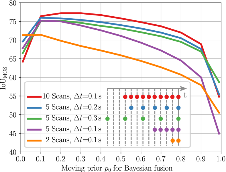
Figure 4: Comparison of $\text{IoU}_{\text{MOS}}$ on the SemanticKITTI [3] validation set using different moving object priors for the binary Bayes filter. The colors indicate variants of our approach using different time horizons and resolutions. The colored dots on the timeline visualize which past scans we input to the model for prediction at time $t$

.

IV-E Ablation Study

To further support our third claim and show the effectiveness of individual proposed components of our approach, we train different variants of our network and evaluate their performance on the validation set. We train all models for up to $60$ epochs and report the best $\text{IoU}_{\text{MOS}}$ on the validation set during training, see Tab. III. For all methods, we compare two prediction strategies: First, a non-overlapping strategy that divides the input sequence into sub-sequences and predicts each sub-sequence independently, see the upper part in Fig. 3. Second, our receding horizon strategy proposed in Sec. III-C, which generates multiple predictions for the same scan and fuses them in a binary Bayes filter (again using a prior of $p_{0}{=}0.25$). We visualize this combination in the lower part of Fig. 3.

In general, we see an improvement of up to $5.4$ percentage points of $\text{IoU}_{\text{MOS}}$ for all models using the proposed receding horizon strategy. More precisely, using the binary Bayes filter with model [A] reduces the number of false negatives by $8.2$% and the number of false positives by $18.9$%. This indicates that the proposed approach successfully integrates more observations into the estimation and is more robust to false predictions due to occlusions or noisy measurements. If we compare the performance of model [A] using $N{=}5$ scans which are $\Delta t{=}0.1$ s apart to the networks trained with larger temporal resolutions of $\Delta t{=}0.2$ s [B] and $\Delta t{=}0.3$ s [C], we again see that the results can be further improved by considering a larger time horizon, see also Sec. IV-D. If the point clouds are not transformed into a common viewpoint, the method [D] is still able to infer moving objects but at a reduced performance of $\text{IoU}_{\text{MOS}}$ ${=}39.9\%$ with Bayesian fusion. This is because the network needs to infer both the ego-motion of the sensor as well as the relative motion of the objects. When only training to predict a single output scan [E], the result is worse and fusing more predictions is not possible since no additional predictions are available. Next, one can see that our method can also achieve moving object segmentation with two scans only [F] but the performance is worse. The best performing model [G] takes $N{=}10$ input scans with a temporal resolution of $\Delta t{=}0.1$ s and fuses the predictions resulting in an $\text{IoU}_{\text{MOS}}$ of $77.2\%$. The results show that we achieve a better moving object segmentation by increasing the time horizon with a combination of processing more scans, increasing the temporal resolution, and using the proposed receding horizon strategy with a binary Bayes filter.

	# Inputs	# Outputs	Poses?	$\Delta t$	$\text{IoU}_{\text{MOS}}$ $\left[\%\right]$
					w/o BF	w/ BF
[A]	$5$	$5$	✓	$0.1$ s	$69.1$	74.5
[B]	$5$	$5$	✓	$0.2$ s	$71.8$	75.6
[C]	$5$	$5$	✓	$0.3$ s	$71.6$	74.9
[D]	$5$	$5$	✗	$0.1$ s	$35.6$	39.9
[E]	$5$	$1$	✓	$0.1$ s	66.5	-
[F]	$2$	$2$	✓	$0.1$ s	$64.9$	69.0
[G]	$10$	$10$	✓	$0.1$ s	$74.3$	77.2

TABLE III: Ablation study on different variants of our approach with and without the proposed receding horizon strategy and Bayesian fusion (BF) using a prior $p_{0}{=}0.25$. We denote the temporal resolution between scans by $\Delta t$. Best results in bold.

IV-F Qualitative Results

Finally, we illustrate that our method predicts actually moving objects in 3D space without the need for geometric post-processing like clustering. We use the model from Sec. IV-B trained on $N{=}10$ scans with a temporal resolution of $\Delta t{=}0.1$ s. In Fig. 5, we show the segmentation of scan $1638$ from the SemanticKITTI [3] validation sequence $08$. We compare the range image-based method LMNet [5] to our sparse voxel-based approach. One can see that despite the geometric-based kNN post-processing, the baseline still shows artifacts and bleeding labels behind the moving car illustrated as red-colored false positives whereas our method directly predicts in the 3D space without boundary effects.

Next, Fig. 6 shows how the prediction changes for a scene in the validation set in which a vehicle stops moving. Since our method does not use any semantic understanding of objects, it only reasons about how the points move in space for the given time horizon. Since the vehicle stops moving to yield at the intersection, our method’s prediction changes from moving to static. The bicyclist in the back is successfully classified as moving. Note that this results in a false negative indicated in blue since the ground truth SemanticKITTI labels consider if an object has moved throughout the data collection and not based on recent movement.

Figure 5: Qualitative comparison of segmentation accuracy. Left: Prediction by range image-based LMNet [5] after kNN post-processing. Right: Our sparse voxel-based approach without further post-processing. Best viewed in color.

Figure 6: Change in moving object segmentation if an object stops moving. Best viewed in color.

IV-G Runtime

With our unoptimized Python implementation, the network requires on average $0.078$ s for predicting moving objects in $10$ scans and $0.047$ s for $5$ scans both using an NVIDIA RTX A5000. Our binary Bayes filter only adds a small overhead of $0.008$ s on average for fusing $10$ predictions and $0.004$ s for fusing $5$ predictions.

V Conclusion

In this paper, we present a novel approach to segment moving objects in 3D LiDAR data. Our method jointly predicts moving objects for all scans in the input sequence and operates using a receding horizon strategy. We report improved performance on the SemanticKITTI moving object segmentation benchmark and show that the approach generalizes well on unseen data. Our proposed receding horizon strategy in combination with a binary Bayes filter allows us to extend the time horizon used for segmenting moving objects and to increase the robustness to false positive and false negative predictions. Currently, we estimate odometry and moving object segmentation separately which can be jointly optimized in future work.

References

- [1] M. Arora, L. Wiesmann, X. Chen, and C. Stachniss. Mapping the Static Parts of Dynamic Scenes from 3D LiDAR Point Clouds Exploiting Ground Segmentation. In Proc. of the Europ. Conf. on Mobile Robotics (ECMR), 2021.
- [2] S.A. Baur, D.J. Emmerichs, F. Moosmann, P. Pinggera, B. Ommer, and A. Geiger. SLIM: Self-Supervised LiDAR Scene Flow and Motion Segmentation. In Proc. of the IEEE/CVF Intl. Conf. on Computer Vision (ICCV), 2021.
- [3] J. Behley, M. Garbade, A. Milioto, J. Quenzel, S. Behnke, C. Stachniss, and J. Gall. SemanticKITTI: A Dataset for Semantic Scene Understanding of LiDAR Sequences. In Proc. of the IEEE/CVF Intl. Conf. on Computer Vision (ICCV), 2019.
- [4] J. Behley and C. Stachniss. Efficient Surfel-Based SLAM using 3D Laser Range Data in Urban Environments. In Proc. of Robotics: Science and Systems (RSS), 2018.
- [5] X. Chen, S. Li, B. Mersch, L. Wiesmann, J. Gall, J. Behley, and C. Stachniss. Moving Object Segmentation in 3D LiDAR Data: A Learning-based Approach Exploiting Sequential Data. IEEE Robotics and Automation Letters (RA-L), 6:6529–6536, 2021.
- [6] X. Chen, B. Mersch, L. Nunes, R. Marcuzzi, I. Vizzo, J. Behley, and C. Stachniss. Automatic Labeling to Generate Training Data for Online LiDAR-Based Moving Object Segmentation. IEEE Robotics and Automation Letters (RA-L), 7(3):6107–6114, 2022.
- [7] X. Chen, A. Milioto, E. Palazzolo, P. Giguère, J. Behley, and C. Stachniss. SuMa++: Efficient LiDAR-based Semantic SLAM. In Proc. of the IEEE/RSJ Intl. Conf. on Intelligent Robots and Systems (IROS), 2019.
- [8] C. Choy, J. Gwak, and S. Savarese. 4D Spatio-Temporal ConvNets: Minkowski Convolutional Neural Networks. In Proc. of the IEEE/CVF Conf. on Computer Vision and Pattern Recognition (CVPR), 2019.
- [9] T. Cortinhal, G. Tzelepis, and E. Aksoy. SalsaNext: Fast Semantic Segmentation of LiDAR Point Clouds for Autonomous Driving. arXiv preprint, 2003.03653, 2020.
- [10] A. Dewan and W. Burgard. DeepTemporalSeg: Temporally Consistent Semantic Segmentation of 3D LiDAR Scans. In Proc. of the IEEE Intl. Conf. on Robotics & Automation (ICRA), 2020.
- [11] M. Everingham, L. Van Gool, C. Williams, J. Winn, and A. Zisserman. The Pascal Visual Object Classes (VOC) Challenge. Intl. Journal of Computer Vision (IJCV), 88(2):303–338, 2010.
- [12] H.W. F. Duerr, M. Pfaller and J. Beyerer. LiDAR-based Recurrent 3D Semantic Segmentation with Temporal Memory Alignment. In Proc. of the Intl. Conf. on 3D Vision (3DV), 2020.
- [13] H. Fan, X. Yu, Y. Ding, Y. Yang, and M. Kankanhalli. PSTNet: Point Spatio-Temporal Convolution on Point Cloud Sequences. In Proc. of the Int. Conf. on Learning Representations (ICLR), 2021.
- [14] H. Fan and Y. Yang. PointRNN: Point Recurrent Neural Network for Moving Point Cloud Processing. arXiv preprint, 1910.08287, 2019.
- [15] Z. Gojcic, O. Litany, A. Wieser, L.J. Guibas, and T. Birdal. Weakly Supervised Learning of Rigid 3D Scene Flow. In Proc. of the IEEE/CVF Conf. on Computer Vision and Pattern Recognition (CVPR), 2021.
- [16] A. Hornung, K. Wurm, M. Bennewitz, C. Stachniss, and W. Burgard. OctoMap: An Efficient Probabilistic 3D Mapping Framework Based on Octrees. Autonomous Robots, 34:189–206, 2013.
- [17] G. Kim and A. Kim. Remove, Then Revert: Static Point Cloud Map Construction Using Multiresolution Range Images. In Proc. of the IEEE/RSJ Intl. Conf. on Intelligent Robots and Systems (IROS), 2020.
- [18] D. Kingma and J. Ba. Adam: A Method for Stochastic Optimization. In Proc. of the Int. Conf. on Learning Representations (ICLR), 2015.
- [19] A. Laddha, S. Gautam, G.P. Meyer, and C. Vallespi-Gonzalez. RV-FuseNet: Range View based Fusion of Time-Series LiDAR Data for Joint 3D Object Detection and Motion Forecasting. arXiv preprint, 2005.10863, 2020.
- [20] X. Liu, C.R. Qi, and L.J. Guibas. FlowNet3D: Learning Scene Flow in 3D Point Clouds. In Proc. of the IEEE/CVF Conf. on Computer Vision and Pattern Recognition (CVPR), 2019.
- [21] X. Liu, M. Yan, and J. Bohg. MeteorNet: Deep Learning on Dynamic 3D Point Cloud Sequences. In Proc. of the IEEE/CVF Intl. Conf. on Computer Vision (ICCV), 2019.
- [22] W. Lu, Y. Zhou, G. Wan, S. Hou, and S. Song. L3-Net: Towards Learning Based LiDAR Localization for Autonomous Driving. In Proc. of the IEEE/CVF Conf. on Computer Vision and Pattern Recognition (CVPR), 2019.
- [23] W. Luo, B. Yang, and R. Urtasun. Fast and Furious: Real Time End-to-End 3D Detection, Tracking and Motion Forecasting with a Single Convolutional Net. In Proc. of the IEEE Conf. on Computer Vision and Pattern Recognition (CVPR), 2018.
- [24] B. Mersch, X. Chen, J. Behley, and C. Stachniss. Self-supervised Point Cloud Prediction Using 3D Spatio-temporal Convolutional Networks. In Proc. of the Conf. on Robot Learning (CoRL), 2021.
- [25] A. Milioto, I. Vizzo, J. Behley, and C. Stachniss. RangeNet++: Fast and Accurate LiDAR Semantic Segmentation. In Proceedings of the IEEE/RSJ Int. Conf. on Intelligent Robots and Systems (IROS), 2019.
- [26] S. Mohapatra, M. Hodaei, S. Yogamani, S. Milz, P. Mäder, H. Gotzig, M. Simon, and H. Rashed. LiMoSeg: Real-time Bird’s Eye View based LiDAR Motion Segmentation. In Proc. of the Intl. Conf. of Computer Vision Theory and Applications (VISAPP), 2022.
- [27] L. Nunes, R. Marcuzzi, X. Chen, J. Behley, and C. Stachniss. SegContrast: 3D Point Cloud Feature Representation Learning through Self-supervised Segment Discrimination. IEEE Robotics and Automation Letters (RA-L), 7(2):2116–2123, 2022.
- [28] F. Pomerleau, P. Krüsiand, F. Colas, P. Furgale, and R. Siegwart. Long-term 3D Map Maintenance in Dynamic Environments. In Proc. of the IEEE Intl. Conf. on Robotics & Automation (ICRA), 2014.
- [29] O. Ronneberger, P.Fischer, and T. Brox. U-Net: Convolutional Networks for Biomedical Image Segmentation. In Medical Image Computing and Computer-Assisted Intervention, volume 9351 of LNCS, pages 234–241. Springer, 2015.
- [30] P. Ruchti and W. Burgard. Mapping with Dynamic-Object Probabilities Calculated from Single 3D Range Scans. In Proc. of the IEEE Intl. Conf. on Robotics & Automation (ICRA), 2018.
- [31] T. Shan, B. Englot, D. Meyers, W. Wang, C. Ratti, and D. Rus. LIO-SAM: Tightly-coupled Lidar Inertial Odometry via Smoothing and Mapping. In Proc. of the IEEE/RSJ Intl. Conf. on Intelligent Robots and Systems (IROS), pages 5135–5142, 2020.
- [32] H. Shi, G. Lin, H. Wang, T.Y. Hung, and Z. Wang. SpSequenceNet: Semantic Segmentation Network on 4D Point Clouds. In Proc. of the IEEE/CVF Conf. on Computer Vision and Pattern Recognition (CVPR), 2020.
- [33] C. Stachniss and W. Burgard. Mobile Robot Mapping and Localization in Non-Static Environments. In Proc. of the National Conference on Artificial Intelligence (AAAI), pages 1324–1329, 2005.
- [34] H. Thomas, B. Agro, M. Gridseth, J. Zhang, and T.D. Barfoot. Self-Supervised Learning of Lidar Segmentation for Autonomous Indoor Navigation. In Proc. of the IEEE Intl. Conf. on Robotics & Automation (ICRA), 2021.
- [35] H. Thomas, C. Qi, J. Deschaud, B. Marcotegui, F. Goulette, and L. Guibas. KPConv: Flexible and Deformable Convolution for Point Clouds. In Proc. of the IEEE/CVF Intl. Conf. on Computer Vision (ICCV), 2019.
- [36] S. Thrun, W. Burgard, and D. Fox. Probabilistic Robotics. MIT Press, 2005.
- [37] I. Tishchenko, S. Lombardi, M.R. Oswald, and M. Pollefeys. Self-Supervised Learning of Non-Rigid Residual Flow and Ego-Motion. In Proc. of the Intl. Conf. on 3D Vision (3DV), 2020.
- [38] M. Toyungyernsub, M. Itkina, R. Senanayake, and M.J. Kochenderfer. Double-Prong ConvLSTM for Spatiotemporal Occupancy Prediction in Dynamic Environments. In Proc. of the IEEE Intl. Conf. on Robotics & Automation (ICRA), 2021.
- [39] D.Z. Wang, I. Posner, and P. Newman. What Could Move? Finding Cars, Pedestrians and Bicyclists in 3D Laser Data. In Proc. of the IEEE Intl. Conf. on Robotics & Automation (ICRA), 2012.
- [40] P. Wu, S. Chen, and D.N. Metaxas. MotionNet: Joint Perception and Motion Prediction for Autonomous Driving Based on Bird’s Eye View Maps. In Proc. of the IEEE/CVF Conf. on Computer Vision and Pattern Recognition (CVPR), 2020.