Diffusion probabilistic modeling of protein backbones in 3D for the motif-scaffolding problem

Abstract

Construction of a scaffold structure that supports a desired motif, conferring protein function, shows promise for the design of vaccines and enzymes. But a general solution to this motif-scaffolding problem remains open. Current machine-learning techniques for scaffold design are either limited to unrealistically small scaffolds (up to length 20) or struggle to produce multiple diverse scaffolds. We propose to learn a distribution over diverse and longer protein backbone structures via an E(3)-equivariant graph neural network. We develop SMCDiff to efficiently sample scaffolds from this distribution conditioned on a given motif; our algorithm is the first to theoretically guarantee conditional samples from a diffusion model in the large-compute limit. We evaluate our designed backbones by how well they align with AlphaFold2-predicted structures. We show that our method can (1) sample scaffolds up to 80 residues and (2) achieve structurally diverse scaffolds for a fixed motif.

1 Introduction

A central task in protein design is creation of a stable scaffold to support a target motif. Here, motifs are structural protein fragments imparting biological function while scaffolds stabilize the motif’s structure. Vaccines and enzymes have already been designed by solving certain instances of this motif-scaffolding problem (Procko et al., 2014; Correia et al., 2014; Jiang et al., 2008; Siegel et al., 2010). However, successful solutions to this problem in the past have necessitated substantial expert involvement and laborious trial and error. Machine learning (ML) offers the hope to automate, and better direct this search. But existing ML approaches face one of two major roadblocks. First, many methods do not build scaffolds longer than about 20 residues. For many motif sizes of interest, the resulting proteins would be smaller than the shortest commonly-studied simple protein folds (35–40 residues) (Gelman & Gruebele, 2014). Second, while other methods may generate longer scaffolds using stochastic search techniques, they require hours of computation to generate a single plausible scaffold (Wang et al., 2022; Anishchenko et al., 2021; Tischer et al., 2020). Moreover, when a plausible scaffold is found, it remains to be experimentally validated. Therefore, it is desirable to return not just a single scaffold but rather a set of scaffolds exhibiting diverse sequences and structural variation to increase the likelihood of success in practice.

In the present work, we demonstrate the promise of a particular generative modeling approach within ML for efficiently returning a diverse set of motif-supporting scaffolds. Generative models have been shown to capture a distribution over diverse protein structures (Lin et al., 2021). But it is not clear how to handle conditioning (on the motif) using these approaches. Diffusion probabilistic models (DPMs) offer a potential alternative; not only do they provide a more straightforward path to handling conditioning, but they have also enjoyed success generating small-molecules in 3D (Hoogeboom et al., 2022). Extending DPMs to protein structures, though, is non-trivial; since proteins are larger than small molecules, modeling proteins requires handling the sequential ordering of residues and long-range interactions. Finally, while existing models often generate distance matrices (Anand & Huang, 2018; Lin et al., 2021), we instead focus on generating a full set of 3D coordinates, which should improve designability in practice. Our resulting model, ProtDiff, is similar to concurrent work on E(3)-equivariant diffusion models for molecules (Hoogeboom et al., 2022), but with modifications specific to protein structure. Moreover, we develop a novel motif-scaffolding procedure based on Sequential Monte Carlo, SMCDiff, that repurposes an unconditionally trained DPM for conditional sampling. We prove that if a DPM matches the data distribution, SMCDiff is guaranteed to provide exact conditional samples in a large-compute limit; this property contrasts with previous methods (Song et al., 2021; Zhou et al., 2021), which we show introduce non-trivial approximation error that impedes performance. Our final motif-scaffolding generative framework, then, has two steps (Fig. 1): first we train ProtDiff to learn a distribution over protein backbones, and then we use SMCDiff with ProtDiff to inpaint arbitrary motifs.

Ours is the first machine-learning method to construct scaffolds longer than 20 residues around motifs — we build up to 80 residues scaffolds on a test case. Beyond our progress on the motif-scaffolding problem, we provide the following technical contributions: (1) we introduce a protein-backbone generative model in 3D – with the ability to generate backbone samples that structurally agree with AlphaFold2 predictions, and (2) we develop a novel conditional sampling algorithm for inpainting.

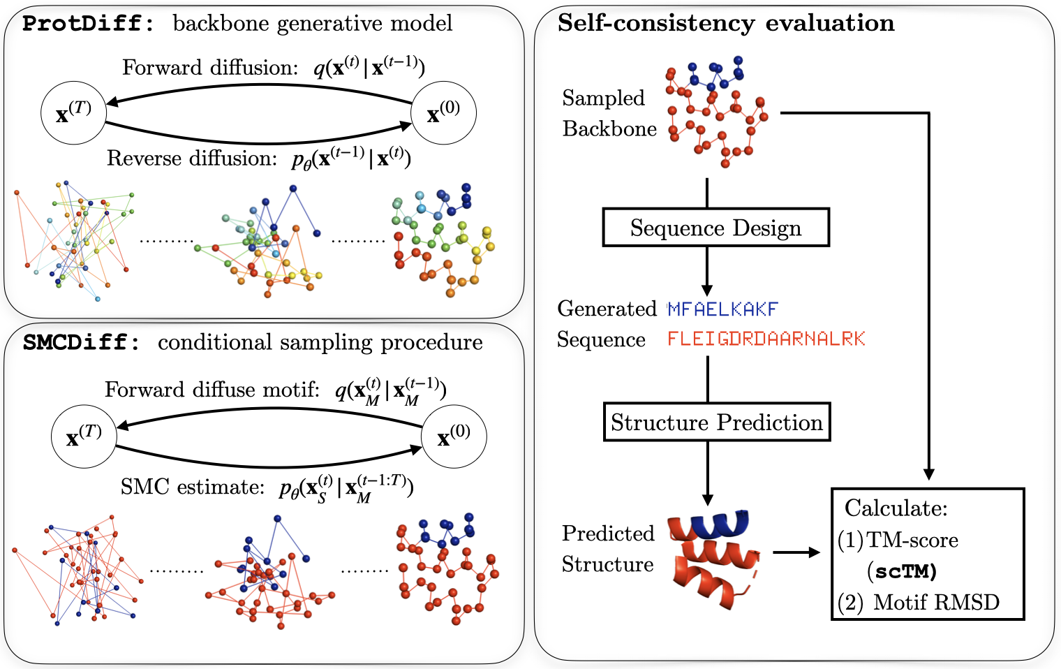
Figure 1: Overview of the conditional generative modeling approach to the motif-scaffolding problem. We train our new protein backbone diffusion model, ProtDiff, to generate realistic protein backbone structures. Next, we run SMCDiff, our conditional sampling algorithm, with ProtDiff to generate scaffolds (colored in red) conditioned on the motif (colored in blue). For self-consistency evaluation, we use a pretrained fixed-backbone sequence-design model (ProteinMPNN (Dauparas et al., 2022)) to generate the scaffold sequence from a sampled backbone. We then input the sequence to a structure prediction model, in our case AlphaFold2 (AF2) (Jumper et al., 2021), to generate the full protein structure from the generated sequence. We compare the backbone of the predicted structure with the original backbone structure using TM-score (Xu & Zhang, 2010) and root-mean-square-distance (RMSD) for the motif.

1.1 Related work

Motif-scaffolding. Past approaches have sought to scaffold a motif with native or prespecified protein fragments, but are limited to finding a suitable match in the Protein Data Bank (PDB) and cannot adapt the scaffold to compensate for slight structural mismatches (Cao et al., 2022; Silva et al., 2016; Yang et al., 2021; Sesterhenn et al., 2020; Linsky et al., 2020). More recently Wang et al. (2022) used pre-trained protein structure prediction networks to recapitulate native scaffolds, but this method failed to generate scaffolds longer than 20 residues and can output only a single candidate scaffold rather than a diverse set. By contrast, our goal is to sample diverse, long scaffolds.

Diffusion models for molecule generation. Several concurrent works have extended equivariant diffusion models to molecule generation. Anand & Achim (2022) extended diffusion models for generation of protein backbone frames and sequences conditioned on secondary structure adjacency matrices. Similarly, Luo et al. (2022) focused on CDR-loop generation using diffusion models conditioned on non-CDR regions of the antibody-antigen. Our method does not require conditioning and is applicable to general proteins. Lee & Kim (2022) approach the same problem as our work but build diffusion models over 2D distances matrices that requires post-processing to produce 3D structures through Rosetta minimization. We demonstrate capability of diffusion models to directly model 3D coordinates of proteins. Hoogeboom et al. (2022) developed an equivariant diffusion model (EDM) for generating small molecules in 3D. However, because EDM does not enforce a spatial ordering of the atoms that compose small molecules, as we describe in Section 5, it does not learn a coherent chain structure as needed in proteins.

Inpainting and conditional sampling in diffusion models. Point-Voxel Diffusion (PVD) (Zhou et al., 2021) is a 3D diffusion model for generating shapes from the ShapeNet dataset. Though trained to generate shapes unconditionally, PVD completes (or inpaints) full shapes when a partial point cloud is fixed during inference. For general diffusion models, Song et al. (2021) proposed an alternative inpainting approach and remarked that this approach produces approximate conditional samples. However, these methods do not provide theoretical guarantees, and when we compare them to SMCDiff, we find that their approximation error impedes performance when applied to motif-scaffolding. Saharia et al. (2022) developed an inpainting diffusion model by training a diffusion model to denoise randomly generated masked regions while unmasked regions were unperturbed. However, their approach requires a detailed data augmentation strategy that does not exist for proteins.

We describe additional related work on protein generative models in Appendix A.

2 Preliminaries

2.1 The motif-scaffolding problem

A protein can be represented by its amino acid sequence and backbone structure. Let $\mathcal{A}$ be the set of 20 genetically-encoded amino acids. We denote the sequence of an $N$-residue protein by $s\in\mathcal{A}^{N}$ and its C-$\alpha$ backbone coordinates in 3D by $\mathbf{x}=[\mathbf{x}_{1},\dots,\mathbf{x}_{N}]^{T}\in\mathbb{R}^{N,3}$. We describe a protein as having a fixed structure that is a function of its sequence, so we may write $\mathbf{x}(s)$. We divide the $N$ residues into the functional motif $\mathcal{M}$ and the scaffold $\mathcal{S},$ such that $\mathcal{M}\cup\mathcal{S}=\{1,2,\dots,N\}.$ The goal is to identify, given the motif structure $\mathbf{x}_{\mathcal{M}}$, sequences $s$ whose structure recapitulates the motif to high precision $\mathbf{x}(s)_{\mathcal{M}}\approx\mathbf{x}_{\mathcal{M}}$. Appendix B discusses several caveats of this simplified framing (e.g. our assumption of static structures).

2.2 Diffusion probabilistic models

Our approach to the motif-scaffolding problem builds on denoising diffusion probabilistic models (DPMs) (Sohl-Dickstein et al., 2015). We follow the conventions and notation set by Ho et al. (2020), which we review here. DPMs are a class of generative models based on a reversible, discrete-time diffusion process. The forward process starts with a sample $\mathbf{x}^{(0)}$ from an unknown data distribution $q$, with density denoted by $q(\mathbf{x}^{(0)}),$ and iteratively adds noise at each step $t$. By the last step, $T$, the distribution of $\mathbf{x}^{(T)}$ is indistinguishable from an isotropic Gaussian: $\mathbf{x}^{(T)}\sim\mathcal{N}(\mathbf{x}^{(T)};0,\mathbf{I}).$ Specifically, we choose a variance schedule $\beta^{(1)},\beta^{(2)},\dots,\beta^{(T)}$, and define the transition distribution at step $t$ as $q(\mathbf{x}^{(t)}\mid\mathbf{x}^{(t-1)})=\mathcal{N}(\mathbf{x}^{(t)};\sqrt{1-\beta^{(t)}}\mathbf{x}^{(t-1)},\beta^{(t)}\mathbf{I})$.

DPMs approximate $q$ with a second distribution $p_{\theta}$ by learning the transition distribution of the reverse process at each $t,$ $p_{\theta}(\mathbf{x}^{(t-1)}\mid\mathbf{x}^{(t)}).$ We follow the conventions set by Ho et al. (2020) in our parameterization and choice of objective. In particular, we take $p_{\theta}(\mathbf{x}^{(t-1)}\mid\mathbf{x}^{(t)})=\mathcal{N}(\mathbf{x}^{(t-1)};\mu_{\theta}(\mathbf{x}^{(t)},t),\beta^{(t)}\mathbf{I})$ with $\mu_{\theta}(\mathbf{x}^{(t)},t)=\frac{1}{\sqrt{\alpha^{(t)}}}\left(\mathbf{x}^{(t)}-\frac{\beta^{(t)}}{\sqrt{1-\bar{\alpha}^{(t)}}}\epsilon_{\theta}(\mathbf{x}^{(t)},t)\right),$ $\alpha^{(t)}:=1-\beta^{(t)}$, and $\bar{\alpha}^{(t)}:=\prod_{s=1}^{t}\alpha^{(t)}.$ We implement $\epsilon_{\theta}(\mathbf{x}^{(t)},t)$ as a neural network. For training, we marginally sample $\mathbf{x}^{(t)}\sim q(\mathbf{x}^{(t)}\mid\mathbf{x}^{(0)})$ from the forward process as $\mathbf{x}^{(t)}=\sqrt{\bar{\alpha}^{(t)}}\mathbf{x}^{(0)}+\sqrt{1-\bar{\alpha}^{(t)}}\epsilon$ and minimize the objective $T^{-1}\sum_{t=1}^{T}\mathbb{E}_{q(\mathbf{x}^{(0)},\mathbf{x}^{(t)})}\left[\|\epsilon-\epsilon_{\theta}(\mathbf{x}^{(t)},t)\|^{2}\right]$ by stochastic optimization (Ho et al., 2020, Algorithm 1). To generate samples from $p_{\theta}(\mathbf{x}^{(0)}),$ we simulate the reverse process. That is, we sample noise for time $T$ as $\mathbf{x}^{(T)}\sim\mathcal{N}(0,\mathbf{I}),$ and then for each $t=T-1,\dots,0,$ we simulate progressively “de-noised” samples as $\mathbf{x}^{(t)}\sim p_{\theta}(\mathbf{x}^{(t)}\mid\mathbf{x}^{(t+1)}).$

3 ProtDiff: A diffusion model of protein backbones in 3D

Implementation of diffusion probabilistic models requires choosing an architecture for the neural network $\epsilon_{\theta}(\mathbf{x}^{(t)},t)$ introduced abstractly in Section 2.2. In this section we describe ProtDiff, which corresponds to the choice of $\epsilon_{\theta}(\mathbf{x}^{(t)},t)$ as a translation and rotation equivariant graph neural network tailored to modeling protein backbones. We leave architectural and input encoding details to Appendix C.

The challenge of modeling points in 3D. The properties and functions of proteins are dictated by the relative geometry of their residues, and are invariant to the coordinate system chosen to encode them. Recent work on neural network modeling of 3D data has found, both theoretically and empirically, that neural networks constrained to satisfy geometric invariances can provide inductive biases that improve generalization and training efficiency (Batzner et al., 2022). Motivated by this observation, we parameterize $\epsilon_{\theta}$ by an equivariant graph neural network (EGNN) (Satorras et al., 2021), which in 3D is equivariant to transformations in the Euclidean group. Xu et al. (2022) proved that if $\epsilon_{\theta}$ is equivariant to a group then $p_{\theta}$ is invariant to the same group.

Tailoring EGNN to protein backbones. We now describe our EGNN implementation, which we tailor to protein backbones and DPMs through the choice of edge and node features. To model every pairwise residue interaction, we represent backbones by a fully connected graph. Each node in the graph is indexed by $n=1,\dots,N,$ and corresponds to a residue. We associate each node with coordinates $\mathbf{x}_{n}\in\mathbb{R}^{3}$ and $D$ features $h_{n}\in\mathbb{R}^{D}.$ For each pair of nodes $n,n^{\prime}$ we define an edge and associate it with edge features. We construct our EGNN by stacking $L$ equivariant graph convolutional layers (EGCL) . Each layer takes node coordinates and features as input, and outputs updated coordinates and features with the first layer taking initial values $(\mathbf{x},h)$. We write the output of EGNN after $L$ layers as $\hat{\mathbf{x}}=\text{EGNN}[\mathbf{x},h]$. In the context of diffusion models, we predict the noise at time $t$ with the following parameterization:

$$\epsilon_{\theta}(\mathbf{x}^{(t)},t)=\hat{\mathbf{x}}-\mathbf{x}^{(t)},\quad\hat{\mathbf{x}}=\text{EGNN}[\mathbf{x}^{(t)},h(t)].$$ (1)

We now describe our choice of node and edge features. Our choice is motivated by the linear chain structure of protein backbones; residues close in sequence are necessarily close in 3D space. To allow this chain constraint to be learned more easily, we fix an ordering of nodes in the graph to correspond to sequence order. We include as edge features positional offsets as done in Ingraham et al. (2019), which we represent using sinusoidal positional encoding features (Vaswani et al., 2017). For node features, we similarly use a sinusoidal encoding of sequence position as well as of the diffusion time step $t$ following Kingma et al. (2021). We additionally process the time encoding to be orthogonal to the positional encoding .

4 SMCDiff: Conditional sampling in diffusion models by particle filtering

The second stage of our generative modeling approach to the motif-scaffolding problem is to sample scaffolds $\mathbf{x}_{\mathcal{S}}^{(0)}$ from $p_{\theta}(\mathbf{x}_{\mathcal{S}}^{(0)}\mid\mathbf{x}_{\mathcal{M}}^{(0)})$. Section 4.1 discusses the intractability of sampling from $p_{\theta}(\mathbf{x}_{\mathcal{S}}^{(0)}\mid\mathbf{x}_{\mathcal{M}}^{(0)})$ exactly and the limitations of a simple approximation introduced by (Song et al., 2021). In Section 4.2, we then frame computation of $p_{\theta}(\mathbf{x}_{\mathcal{S}}^{(0)}|\mathbf{x}_{\mathcal{M}}^{(0)})$ as a sequential Monte Carlo (SMC) problem (Doucet et al., 2001) and approximate it with a particle filtering algorithm (Algorithm 1).

4.1 The challenge of conditional sampling and the error of the replacement method

The conditional distributions of a DPM are defined implicitly through the steps of the reverse process. We may write the conditional density explicitly as

$$p_{\theta}(\mathbf{x}_{\mathcal{S}}^{(0)}\mid\mathbf{x}_{M}^{(0)})\propto p_{\theta}(\mathbf{x}_{\mathcal{S}}^{(0)},\mathbf{x}_{M}^{(0)}) =p_{\theta}(\mathbf{x}^{(0)})=\int p_{\theta}(\mathbf{x}^{(T)})\prod_{t=0}^{T-1}p_{\theta}(\mathbf{x}^{(t)}\mid\mathbf{x}^{(t+1)})d\mathbf{x}^{(1:T)}.$$

However, the high-dimensional integral on the right-hand side above is intractable (both analytically and numerically) to compute.

Algorithm 1 SMCDiff: Particle filtering for conditionally sampling from unconditional diffusion models

1:Input: $\mathbf{x}_{\mathcal{M}}^{(0)}$ (motif), $K$ (# particles)

2:// Forward diffuse motif

3:$\breve{\mathbf{x}}_{\mathcal{M}}^{(1:T)}\sim q(\mathbf{x}_{\mathcal{M}}^{(1:T)}\mid\mathbf{x}_{\mathcal{M}}^{(0)})$

4:

5:// Reverse diffuse particles

6:$\forall k,\ \mathbf{x}_{k}^{(T)}\overset{i.i.d.}{\sim}p_{\theta}(\mathbf{x}^{(T)})$

7:for $t=T,\dots,1$ do

8:     // Replace motif

9:     $\forall k,\ \mathbf{x}_{k}^{(t)}\leftarrow[\breve{\mathbf{x}}_{\mathcal{M}}^{(t)},\mathbf{x}_{\mathcal{S},k}^{(t)}]$

10:

11:     // Re-weight based on $\breve{\mathbf{x}}_{\mathcal{M}}^{(t-1)}$

12:     $\forall k,\ w_{k}^{(t)}\leftarrow p_{\theta}(\breve{\mathbf{x}}_{\mathcal{M}}^{(t-1)}\mid\mathbf{x}_{k}^{(t)})$

13:     $\forall k,\ \tilde{w}_{k}^{(t)}\leftarrow w_{k}^{(t)}/\sum_{k^{\prime}=1}^{K}w_{k^{\prime}}^{(t)}$

14:     $\tilde{\mathbf{x}}_{1:K}^{(t)}\sim\texttt{Resample}(\tilde{w}_{1:K}^{(t)},\mathbf{x}_{1:K}^{(t)})$

15:

16:     // Propose next step

17:     $\forall k,\ \mathbf{x}_{k}^{(t-1)}\overset{indep.}{\sim}p_{\theta}(\mathbf{x}^{(t-1)}\mid\tilde{\mathbf{x}}_{k}^{(t)})$

18:end for

19:Return $\mathbf{x}_{\mathcal{S},1:K}^{(0)}$

To overcome this intractability, we build on the work of Song et al. (2021), who introduced a practical algorithm that generates approximate conditional samples. This strategy is to (1) forward diffuse the conditioning variable to obtain $\mathbf{x}_{\mathcal{M}}^{(1:T)}\sim q(\mathbf{x}_{\mathcal{M}}^{(1:T)}\mid\mathbf{x}_{\mathcal{M}}^{(0)}),$ and then (2) for each $t,$ sample $\mathbf{x}_{\mathcal{S}}^{(t)}\sim p_{\theta}(\mathbf{x}_{\mathcal{S}}^{(t)}\mid\mathbf{x}_{\mathcal{M}}^{(t+1)},\mathbf{x}_{\mathcal{S}}^{(t+1)}).$ We call this approach the replacement method (following Ho et al. (2022)) and make it explicit in Appendix Algorithm 2. However, in D.1 we show that the replacement method introduces irreducible approximation error that cannot be eliminated by making $p_{\theta}$ more expressive. Additionally, although this approximation error is not analytically tractable in general, we show in Corollary D.2 the dependence of this error on the covariance of $\mathbf{x}_{\mathcal{M}}^{(0)}$ and $\mathbf{x}_{\mathcal{S}}^{(0)}$ in the case that $q(\mathbf{x}_{\mathcal{M}}^{(0)},\mathbf{x}_{\mathcal{S}}^{(0)})$ is bivariate Gaussian.

4.2 Conditional sampling is a sequential Monte Carlo problem

We next frame approximation of $q(\mathbf{x}_{\mathcal{S}}^{(0)}\mid\mathbf{x}_{\mathcal{M}}^{(0)})$ as a sequential Monte Carlo problem that we may solve by particle filtering. Intuitively, particle filtering addresses a limitation of the replacement method: the failure at each time $t$ to look beyond the current step to the less-noised motif $\mathbf{x}_{\mathcal{M}}^{(t-1)}$ when sampling $\mathbf{x}_{\mathcal{S}}^{(t)}\sim p_{\theta}(\mathbf{x}_{\mathcal{S}}^{(t)}\mid\mathbf{x}^{(t+1)}).$ Our key insight is that because $p_{\theta}(\mathbf{x}_{\mathcal{M}}^{(t-1)}\mid\mathbf{x}^{(t)})$ provides a mechanism to assess the likelihood of $\mathbf{x}_{\mathcal{M}}^{(t-1)}$, we can prioritize noised scaffolds that are more consistent with the motif. Particle filtering leverages this mechanism to provide a sequence of discrete approximations to each $p_{\theta}(\mathbf{x}_{\mathcal{S}}^{(t)}\mid\mathbf{x}_{\mathcal{M}}^{(t-1:T)})$ that look ahead by this extra step. Finally, at $t=0$ we have an approximation to $p_{\theta}(\mathbf{x}_{\mathcal{S}}^{(0)}\mid\mathbf{x}_{\mathcal{M}}^{(0:T)}).$ Then, using 4.1 below, we can obtain an approximate sample from $q(\mathbf{x}_{\mathcal{S}}^{(0)}\mid\mathbf{x}_{\mathcal{M}}^{(0)}).$ This framing permits the application of standard particle filtering algorithms (Doucet et al., 2001). Algorithm 1 summarizes an implementation of this procedure that uses residual resampling (Doucet & Johansen, 2009) to mitigate the collapse of the sequential approximations into point masses. SMCDiff provides a tunable trade-off between computational cost and statistical accuracy through the choice of the number of particles $K$. In our next proposition we make this trade-off explicit.

Proposition 4.1.

Suppose that $p_{\theta}$ exactly matches the forward diffusion process such that for every $\mathbf{x}^{(t+1)},\,p_{\theta}(\mathbf{x}^{(t)}\mid\mathbf{x}^{(t+1)})=q(\mathbf{x}^{(t)}\mid\mathbf{x}^{(t+1)})$ and consider any motif $\mathbf{x}_{\mathcal{M}}^{(0)}.$ Let $\mathbf{x}_{\mathcal{S},K}$ be a particle chosen at random from the output of Algorithm 1 with $K$ particles. Then $\mathbf{x}_{\mathcal{S},K}$ converges in distribution to $q(\mathbf{x}_{\mathcal{S}}^{(0)}\mid\mathbf{x}_{\mathcal{M}}^{(0)})$ as $K$ goes to infinity.

The significance of 4.1 is that it guarantees Algorithm 1 can provide arbitrarily accurate conditional samples provided an accurate diffusion model and large enough compute budget (determined by the number of particles). To our knowledge, SMCDiff is the first algorithm for asymptotically exact conditionally sampling from unconditional DPMs. Our proof of the proposition, which we leave to Appendix D, is obtained from an application of standard asymptotics for particle filtering (Chopin & Papaspiliopoulos, 2020, Proposition 11.4).

5 Experiments

We empirically demonstrate the ability of our method to scaffold motifs and sample protein backbone structures. We describe our procedure for evaluating backbone designs in Section 5.1. We demonstrate the promise of our method for the motif-scaffolding problem in Figure 2. And we investigate our method’s strengths and weaknesses via experiments in unconditional sampling in Figure 4. We train a single instance of ProtDiff and use it across all of our experiments. For simplicity, we limited our training data to single chain proteins taken from PDB that are no longer than 128 residues. See Appendix F for training details.

Baselines. As mentioned in Section 1.1, Wang et al. (2022) is the only prior machine learning work to address the motif-scaffolding problem. We do not compare against this as a baseline because no stable implementation was available at the time of writing. The most closely related method for unconditional sampling with available software is trDesign (Anishchenko et al., 2021), but this method does not allow specification of a motif. The ML method most similar to ProtDiff is the concurrently developed equivariant diffusion model (EDM) proposed by Hoogeboom et al. (2022). Like ProtDiff, EDM uses a densely connected EGNN architecture but without sequence-distance edge features. Consequently, it does not impose any sequence order, and therefore does not yield a way to relate generated coordinates to a backbone chain.

5.1 In silico evaluation of designed backbones

While experimental validation via X-ray crystallography remains the gold standard for evaluating computationally designed proteins, recent work (Wang et al., 2022; Lin et al., 2021) has proposed to leverage highly accurate protein structure prediction neural networks as an in silico proxy for true structure. More specifically, Wang et al. (2022) jointly design protein sequence and structure, and validate by comparing the design and AlphaFold2 (AF2) (Jumper et al., 2021) predicted structures. Here, our goal is to assess the quality of scaffolds generated independent of a specific sequence, so we treat fixed backbone sequence design as a downstream step as in Lin et al. (2021).

Our evaluation with AF2 is as follows. For each generated scaffold we use a C-$\alpha$ only version of ProteinMPNN (Dauparas et al., 2022) with a temperature of 0.1 to sample 8 amino acid sequences likely to fold to the same backbone structure. We then run AF2 with the released CASP14 weights and 15 recycling iterations. We do not include a multiple sequence alignment as an input to AF2. Our choice of utilizing ProteinMPNN and AF2 (without MSAs) is motivated by their empirical success in various de novo protein design tasks and the ability to recapitulate native proteins (Dauparas et al., 2022; Bennett et al., 2022). To assess unconditionally sampled scaffolds, we then evaluate the agreement of our backbone sample with the AF2 predicted structures using the maximum TM-score (Zhang & Skolnick, 2005) across all generated sequences which we refer to as scTM, for self-consistency TM-score. To assess whether prospective scaffolds generated support a motif, we compute the root mean squared distances (RMSD) of the desired and predicted motif coordinates after alignment and refer this metric as the motif RMSD. Appendix Algorithm 4 outlines the exact steps.

Because a TM-score > 0.5 indicates that two structures have the same fold (Zhang & Skolnick, 2005), we say that a backbone is designable if scTM > 0.5. The ability for AF2 to reproduce the same backbone from an independently designed sequence is evidence a sequence can be found for the starting structure. To verify this is a reasonable cutoff, we analyzed scTM over our training set and found 87% to be designable.

5.2 Motif-scaffolding via conditional sampling

We evaluated our motif-scaffolding approach (combining SMCDiff and ProtDiff) on motifs extracted from existing proteins in the PDB and found that our approach can generate long and diverse scaffolds that support these motifs.

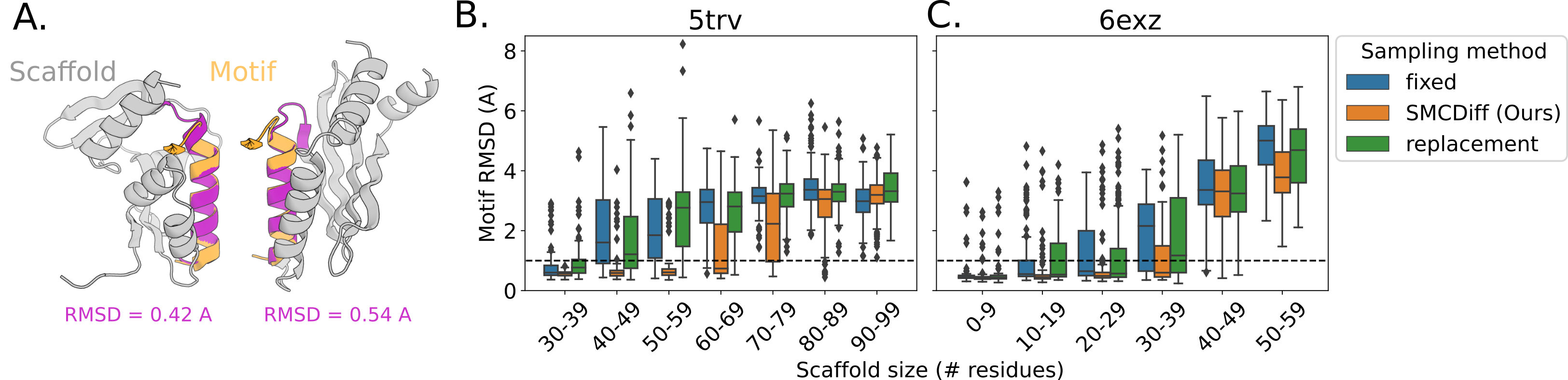
Figure 2: Motif-scaffolding case studies. (A) Example of two scaffold structures generated around a segment of 5trv. Orange: desired input motif, Grey: AlphaFold-predicted structure of two scaffolds, with the motif highlighted (purple). Both scaffolds were sampled using SMCDiff with scTM > 0.5. (B,C) Motif RMSD for 5trv and 6exz test cases, its dependence on scaffold size, and comparison of SMCDiff to two naive inpainting methods (fixed, replacement).

We chose to first evaluate on motifs extracted from proteins present in the training set because we knew that at least one stabilizing scaffold exists. We considered 2 examples taken from the PDB with IDs 6exz and 5trv, which are 69 and 118 residues long, respectively. We chose these examples due to their high secondary structure composition while being representative of the shortest and longest lengths seen during training. For each structure, we chose a 15–25 residue helical segment as the motif (see Appendix H for details). The remainder of each protein is one possible supporting scaffold. We sought to assess if we could recover this and other scaffolds with the same size and motif placement.

Based on prior work (Wang et al., 2022), we expected that building larger scaffolds around a motif would be more challenging than building smaller scaffolds. To assess this length dependence, we expanded the segment of used as the motif when running SMCDiff by including additional residues on each side. In each case, though, we compute the motif RMSD over the minimal motif. In Figure 2B, we present motif-scaffolding performance and its dependence on scaffold size for 5trv, the longer of the two test proteins. For the 5trv test case, the lower quartile of the motif RMSD for SMCDiff is below 1Å for scaffolds up to 80 residues. Since 1Å is atomic-level resolution, we conclude that our approach can succeed in this length range.

Figure 2A provides a visualization of our method’s capacity to generate long and diverse scaffolds. The figure depicts two dissimilar scaffolds of lengths 34 and 54 produced by SMCDiff with 64 particles. Both scaffolds are designable and agree with AF2 (scTM > 0.5). Diversity is particularly evident in the different orderings of secondary structures.

Figure 2B compares SMCDiff to two naive inpainting methods, fixed and replacement. In fixed, the motif is fixed for every timestep $t,$ and the reverse diffusion is applied only to the scaffold (as done by Zhou et al. (2021)); replacement is the method described in Section 4. In contrast to SMCDiff, these baselines fail to generate a successful scaffolds longer than 50 residues on 5trv, as determined by the location of their lower quartiles.

We next applied these three inpainting methods to harder targets in order to measure generalization to out-of-distribution and more difficult motifs comprising of dis-contiguous regions and loops. We consider a motif obtained from the respiratory syncytial virus (RSV) protein and calcium binding EF-hand motif, both of which are not in the training dataset. RSV is known to be difficult due to its composition of helical, loop, and sheet segments, while EF-hand is a dis-contiguous loop motif found in a calcium binding protein. More details about both motifs can be found in Wang et al. (2022); there the authors report the only known successful scaffold of these motifs but they attain it with a computationally intensive hallucination approach. We found that our method failed to generate scaffolds predicted to recapitulate the motif (Appendix H); however, SMCDiff provided smaller median motif RMSDs than the other two inpainting methods.

Compute cost. The computation of SMCDiff with 64 particles is approximately 2 minutes per independent sample, while alternative methods fixed and replacement can produce 64 independent samples in the same time. By contrast, the hallucination approach of Wang et al. (2022) involves running a Markov chain for thousands of steps, and has runtime on the order of hours for a single sample (Anishchenko et al., 2021).

5.3 Unconditional sampling

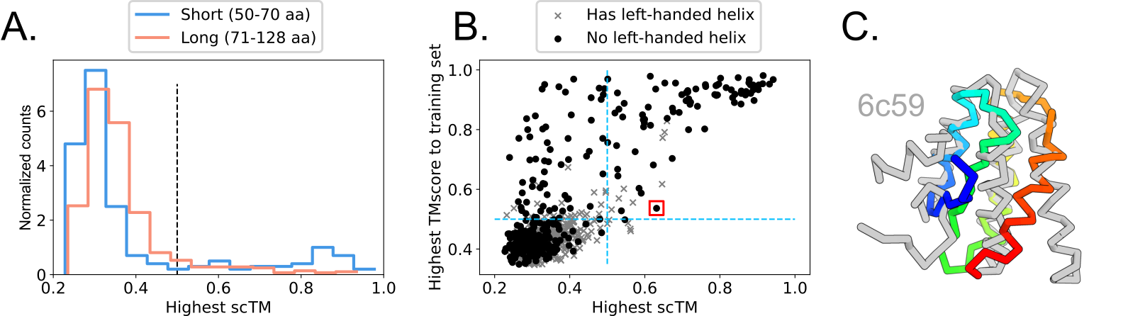
Figure 3: Protein backbone samples from ProtDiff. (A) Density plot of scTM for different length categories (50–70, 70–128). The dashed line at scTM = 0.5 indicates the threshold of “designability”, points to the right are considered “designable” (see text). (B) Scatter plot of scTM and the highest TM-score of each sample to all of PDB. Points represented as a grey “$\times$” are detected to contain an (invalid) left-handed helix. Dashed lines indicate thresholds scTM = 0.5. (C) Example of a designable backbone sample (rainbow) with scTM > 0.5 (boxed in red in panel B) to its closest PDB example (6c59, grey) with a TM-score of 0.54.

We next investigate the origins of the diversity seen in Figure 2 by analyzing the diversity and designability of ProtDiff samples without conditioning on a motif.

We first check that ProtDiff produces designable backbones. To do this, we generated 10 backbone samples for each length between 50 and 128 and then calculated scTM for each sample. In Fig. 3A, we find that 11.8% of samples have scTM > 0.5. However, the majority of backbones do not pass this threshold. We also observe designability has strong dependence on length since we expect that longer proteins are harder to model in 3D and design sequences for. We separated the lengths below 128 residues into two categories and refer to them as short (50–70) and long (70–128). Our results in Figure 3A indicate 17% of designs in the short category are designable vs. 9% in the long category. In Figure 13, we present a structural clustering of these designable backbones; we find that these backbones exhibit diverse topologes.

We next sought to evaluate the ability of ProtDiff to generalize beyond the training set and produce novel backbones. In Figure 3B each point represents a backbone sample from ProtDiff. The horizontal coordinate of a point is the scTM, and the vertical coordinate is the minimum TM-score across the training set. We found a strong positive correlation between scTM and this minimum TM-score, indicating that many of the most designable backbones generated by ProtDiff were a result of training set memorization. However, if the model were only memorizing the training set, we would see TM-scores consistently near 1.0; the range of scores in Figure 3B indicate this is not the case – and the model is introducing a degree of variability. Figure 3C gives an example of backbone with scTM > 0.5 that appears to be novel. Its closest match in the PDB has TM-score = 0.54.

Fig. 3B illustrates a limitation of our method: many of our sampled backbones are not designable. One contributing factor is that ProtDiff does not handle chirality. Hence ProtDiff generates backbones with the wrong handedness, which cannot be realized by any sequence. Fig. 3B shows that 45% of all backbone samples had at least one incorrect, left-handed helix. Of these, most have scTM < 0.5. We describe calculating left-handed helices in Appendix G.

Fig. 4 illustrates an interpolation between two samples, showing how ProtDiff’s outputs change as a function of the noise used to generate them. To generate these interpolations, we pick two backbone samples that result in different folds. For independent samples generated with noise $\epsilon^{(0:T)}$ and $\tilde{\epsilon}^{(0:T)}$ we interpolate with noise set to $\sqrt{\alpha}\epsilon^{(0:T)}+\sqrt{1-\alpha}\tilde{\epsilon}^{(0:T)}$ for $\alpha$ between 0 and 1. The depicted values of $\alpha$ are chosen to highlight transition points with full interpolations included in Section H.3. A future direction is to exploit the latent structure of ProtDiff to control backbone topology.

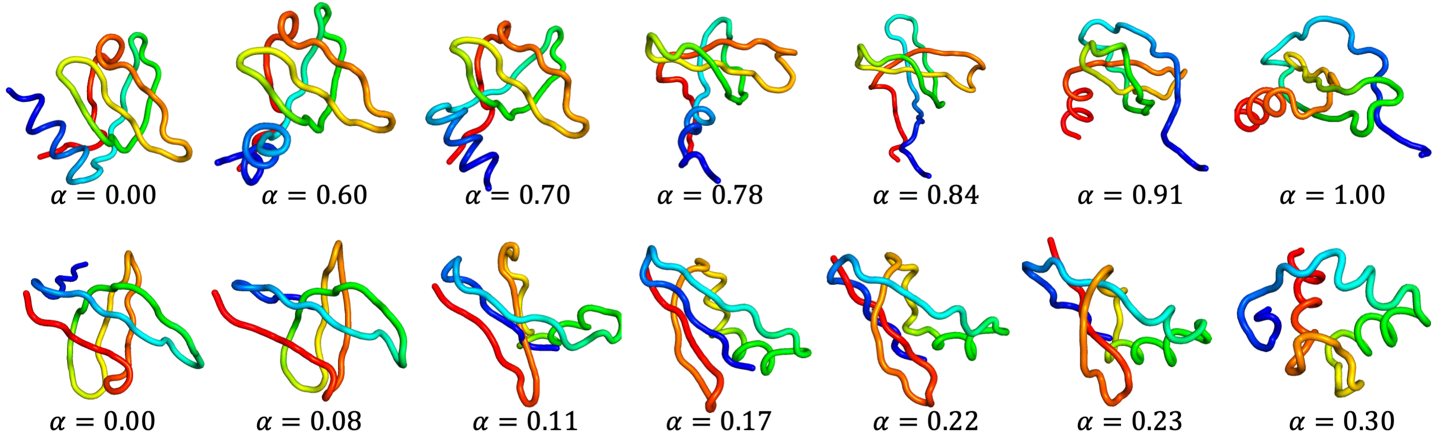
Figure 4: Interpolations between ProtDiff samples demonstrating the diversity of backbones captured. Top: 64-residue example. Bottom: 56-residue example. ProtDiff samples are determined by the Gaussian noise across all steps, $\epsilon^{(0:T)}.$

6 Discussion

The motif-scaffolding problem has applications ranging from medicine to material science (King et al., 2012), but remains unsolved for many functional motifs. We have created the first generative modeling approach to motif-scaffolding by developing ProtDiff, a diffusion probabilistic model of protein backbones, and SMCDiff, a procedure for generating scaffolds conditioned on a motif. Although our experiments were limited to a small set of proteins, our results demonstrate that our procedure is the first capable of generating diverse scaffolds longer than 20 residues with computation time reliably on the order of minutes or less. Our work demonstrates the potential of machine learning methods to be applied in realistic protein design settings.

General conditional sampling. SMCDiff is applicable to generic DPMs and is not limited to only proteins and motif-scaffolding. While we do not make claims of SMCDiff outperforming state-of-the-art conditional diffusion models on other tasks such as image generation, we demonstrate a clear advantage of SMCDiff over the replacement method on a toy task of inpainting MNIST images in Appendix I. Extending SMCDiff outside of motif-scaffolding is outside the scope of the present work, but the advantages of a single model for both unconditional and conditional generation warrants additional research.

Modeling limitations. Our present results do not indicate our procedure can generalize to motifs that are not present in the training set. We believe improvements in protein modeling could provide better inductive biases for generalization. ProtDiff, based on EGNN, is reflection equivariant since it only sees pairwise distances between 3D C-$\alpha$ coordinates. Additionally, ProtDiff does not explicitly model primary sequence or side-chains. Hoogeboom et al. (2022) demonstrate the benefits of modeling sequence information in small molecules; joint modeling sequence and structure in a single model could improve the designability of protein scaffolds and backbones as well.

Data limitations. We remarked our training set is small due to filtering based on length and oligometry (using only monomeric proteins). Scaling up to longer proteins opens up thousands more examples from the PDB, but in preliminary experiments has proven challenging. Lastly, further development and comparison of methods for motif scaffolding will benefit from standard evaluation benchmarks. Developing a benchmark proved to be difficult since motifs are not labeled in protein databases. It will be important to gather motifs of biological importance in order to guide ML method development towards real-world applications. Because no such benchmarks exist, developing them is a valuable direction for future work.

Acknowledgements

The authors thank Octavian-Eugen Ganea, Hannes Stärk, Wenxian Shi, Felix Faltings, Jeremy Wohlwend, Nitan Shalon, Gabriele Corso, Sean Murphy, Wengong Jin, Bowen Jing, Renato Berlinghieri, John Yang, and Jue Wang for helpful discussion and feedback. We thank Justas Dauparas for access to an early version of ProteinMPNN. We dedicate this work in memory of Octavian-Eugen Ganea who initiated the project by connecting all the authors.

BLT and JY were supported in part by NSF-GRFP. BLT and TB were supported in part by NSF grant 2029016 and an ONR Early Career Grant. JY, RB, and TJ acknowledge support from NSF Expeditions grant (award 1918839: Collaborative Research: Understanding the World Through Code), Machine Learning for Pharmaceutical Discovery and Synthesis (MLPDS) consortium, the Abdul Latif Jameel Clinic for Machine Learning in Health, the DTRA Discovery of Medical Countermeasures Against New and Emerging (DOMANE) threats program, the DARPA Accelerated Molecular Discovery program and the Sanofi Computational Antibody Design grant. DT and DB were supported with funds provided by a gift from Microsoft. DB was additionally supported by the Audacious Project at the Institute for Protein Design, the Open Philanthropy Project Improving Protein Design Fund, an Alfred P. Sloan Foundation Matter-to-Life Program Grant (G-2021-16899) and the Howard Hughes Medical Institute.

Part I Appendix

Appendix A Additional related work

We next cover additional related work on generative models of proteins sequence and structure, beyond the discussion in Section 1.1. Following the success of deep language models, Ferruz et al. (2022) developed protein sequence models to generate new proteins, but these models do not allow specification of structural motifs. Another class of methods, referred to as fixed backbone sequence design (Fleishman et al., 2011; Ingraham et al., 2019; Xiong et al., 2020; McPartlon et al., 2022; Hsu et al., 2022), attempts to solve the problem of identifying a sequence that folds into any given designable backbone structure. In the present work, we utilize a particular sequence design method, ProteinMPNN (Dauparas et al., 2022), but in principle any other fixed-backbone sequence design method could be used in its place. Anand & Huang (2018); Lin et al. (2021); Wu et al. (2021) propose generative adversarial networks, variational autoencoders, and energy-based models, respectively, on distance matrices, but these approaches (1) do not generate backbones compatible with a specified motif and (2) rely on an unwieldy optimization step to translate the distance matrix into backbone coordinates. Other authors use neural net (Tischer et al., 2020; Anishchenko et al., 2021; Wang et al., 2022; Huang et al., 2022; Wu et al., 2021), but require a computationally challenging conformational landscape exploration.

Appendix B Problem assumptions and modeling heuristics

The formulation of the motif-scaffolding problem presented in Section 2.1 makes several simplifying assumptions, and our modeling approach relies on several heuristics. We describe these assumptions and heuristics in what follows, and comment on how they might be addressed by further methodological developments. But we first describe an illustrative example of an instance of motif scaffolding.

Protein sequence-structure relationship. Generally speaking, a protein’s sequence encodes an ensemble of conformations, populated to different degrees at biological temperatures. Anfinsen’s hypothesis states that the ground state conformation is thermodynamically accessible (Anfinsen, 1973), providing a mapping from sequence to a unique (ground state) structure. In practice, the ground state structures make up the vast majority of experimentally determined protein conformations, as over 95% of structures in the Protein Data Bank (PDB) are collected at cryogenic temperatures (Fraser et al., 2011). Thus we simplify our problem by saying that a sequence uniquely maps to a static structure (i.e. the ground state structure). However, violations of this assumption arise in some PDB structures as a result of (1) of context specific determinants of structure such as post-translational modifications and environmental factors including pH, binding partners, and salts, as well as (2) thermodynamic inaccessibility of the ground state.

Motif sequence and side-chains. As stated in Section 2.1, we assume we may represent a functional motif by the coordinates of its C-$\alpha$ atoms. However, the biochemical functions of proteins depend not only on backbone structure, but also on side-chains. For example, the activity of many enzymes is imparted by triplets of residues, known as catalytic triads, whose ability to catalyze reactions depends on the spatial organization of side-chain atoms. Our problem statement and subsequent evaluation scheme are agnostic to the amino acid identity of motif residues, let alone side-chain positioning. A more complete representation of a motif would include the side-chain identities (i.e. the amino acid sequence) and side-chain atom coordinates.

Scaffold length and motif placement. We have additionally assumed that the size of scaffolds and the indices of motif residues within the backbone chain, $\mathcal{M},$ are known a priori. However, in practice satisfactory scaffolds could have different lengths and different motif placements, and typically it is not known a priori what lengths and placements will be best. Previous works have addressed this challenge through brute force by sampling multiple lengths and placements, and relied on post-hoc filtering to identify the most promising scaffolds (Wang et al., 2022; Yang et al., 2021). Subsequent work on ML methods could potentially generalize beyond this assumption to efficiently sample appropriate scaffold lengths and motif placements.

Sequence and side-chain modeling. ProtDiff models only the backbone coordinates and leaves sequence design to a subsequent stage, for which we have used ProteinMPNN. A more complete representation of a proteins could include both sequence and structure (where structure can be divided into the backbone and side-chain atom coordinates). To model sequence, we rely on a separately trained neural network, ProteinMPNN, but this is not ideal. Unless ProtDiff produces perfect backbones, one would expect the backbone samples of ProtDiff to present a substantial domain shift when used as input for ProteinMPNN.

3D backbone representation. In this work, we represent a protein structure using the C-$\alpha$ coordinates of every residue along the backbone. However, this representation is coarse-grained and ignores additional backbone atomic coordinates, namely the backbone carbon and nitrogen atoms. Dauparas et al. (2022) observed additionally modeling the heavy atoms of the backbone nitrogen and carbon atoms along with the C-$\beta$ of every residue (to capture side-chain information) improved performance (by sequence recovery) for fixed-backbone sequence design. We hypothesize modeling additional coordinates of every residue would also improve designability performance of ProtDiff. Constraining ProtDiff to place the remaining atoms in the correct orientation could help enforce correct chirality and mitigate chain breaks.

Appendix C Additional ProtDiff details

As a reminder from Section 3, each node in the graph is indexed by $n=1,\dots,N$ and corresponds to a residue with coordinates $\mathbf{x}_{n}\in\mathbb{R}^{3}$ and node features $h_{n}\in\mathbb{R}^{D}$. For each pair of nodes $n,n^{\prime}$ we define an edge and associate it with edge features $a_{nn^{\prime}}\in\mathbb{R}^{D}$. Our neural network to predict $\epsilon_{\theta}$ is an instance of EGNN composed of multiple EGCL layers . We recount details of EGCL and then discuss construction of edge and node features, $a_{nn^{\prime}}$ and $h_{n}$.

Equivariant graph convolution layers (EGCL). Each layer $l=1,\dots,L$ defines an update as $(\mathbf{x}^{l},h^{l})=\text{EGCL}[\mathbf{x}^{l-1},h^{l-1}]$ where for each node $n$

$$\mathbf{x}_{n}^{l}=\mathbf{x}_{n}^{l-1}+\sum_{{n^{\prime}}\neq n}\vec{\omega}_{nn^{\prime}}\cdot\phi_{\mathbf{x}}(h_{n}^{l-1},h_{n^{\prime}}^{l-1},d_{n{n^{\prime}}},a_{n{n^{\prime}}})\quad\text{and}\quad h_{n}^{l}=\phi_{h}(h_{n}^{l-1},m_{n}),\quad\text{for}$$

$$\vec{\omega}_{nn^{\prime}}=\frac{\mathbf{x}_{n}^{l-1}-\mathbf{x}_{n^{\prime}}^{l-1}}{\sqrt{d_{nn^{\prime}}}+\gamma},\quad m_{n}=\sum_{n^{\prime}\neq n}\phi_{e}(h_{n}^{l-1},h_{n^{\prime}}^{l-1},d_{n{n^{\prime}}},a_{nn^{\prime}}),\text{ and }d_{nn^{\prime}}=\|\mathbf{x}_{n}^{l-1}-\mathbf{x}_{n^{\prime}}^{l-1}\|_{2}^{2}.$$

$\phi_{e},\phi_{h}$, and $\phi_{\mathbf{x}}$ are fully connected neural networks, and $\gamma$ is a small positive constant included for numerical stability. The first EGCL layer takes in initial node embeddings, $h^{0}$ while edge embeddings, $a_{nn^{\prime}}$, are kept fixed throughout.

Initial node and edge embeddings. Each edge between two residues indexed in the sequence by $(n,n^{\prime})$ is featurized with $D$ features obtained through a sinusoidal encoding of its relative offset:

$$a_{nn^{\prime}}=\begin{bmatrix}\varphi(n-n^{\prime},1)\\ \vdots\\ \varphi(n-n^{\prime},D)\end{bmatrix},\text{ where }\ \varphi(x,k)=\begin{cases}\text{sin}\left(x\cdot\pi/N^{2\cdot k/D}\right),&k\mod 2=0\\ \text{cos}\left(x\cdot\pi/N^{2\cdot(k-1)/D}\right),&k\mod 2=1.\end{cases}$$

For node features, we similarly use a sinusoidal encoding of sequence position as well as of the diffusion time step $t$ as

$$h_{n}(t)=\begin{bmatrix}\varphi(n,1)\\ \vdots\\ \varphi(n,D)\end{bmatrix}+R\begin{bmatrix}\varphi(t,1)\\ \vdots\\ \varphi(t,D)\end{bmatrix},\$$

where $R$ is a $D\times D$ orthogonal matrix chosen uniformly at random. Intuitively, applying $R$ transforms the time encoding to be orthogonal to the positional encoding.

Coordinate scaling While protein structures are typically parameterized in Angstroms, we transform the input protein coordinates to be in nanometers rather by dividing by 10. This scaling brings the backbones to a spatial scale similar to the reference distribution at which the forward noising process is stationary, a unit variance isotropic Gaussian. Importantly, the distribution of the final step $T$ is indistinguishable from an isotropic Gaussian (Supplementary Fig. 5.)

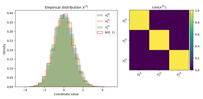
Figure 5: Distribution of $x^{(T)}$ after centering and scaling $x^{(0)}$ to nanometers.

Appendix D Conditional sampling: SMCDiff details and supplementary proofs

We here provide additional details related to SMCDiff and the replacement method described in Section 4. Details of the replacement method (Song et al., 2021) and our analysis of its error are in Section D.1. Section D.2 provides details of our sampling method, SMCDiff, including (1) a proof of 4.1 and (2) details of the residual resampling step. We leave technical proofs and lemmas to Section D.3.

Notation. In the following, we require notation that is more precise than in previous sections. For each $t=0,\dots,T,$ we let $q_{t}(\cdot)$ and $p_{t}(\cdot)$ denote the density functions of $\mathbf{x}^{(t)}$ according to the forward process and to our neural network approximation of the reverse process, respectively. We denote densities restricted to the motif and scaffold with subscripts $\mathcal{M}$ and $\mathcal{S}.$ For example, we here write $p_{\mathcal{M},t}(\mathbf{x}_{\mathcal{M}}^{(t)})$, whereas we wrote $p_{\theta}(\mathbf{x}_{\mathcal{M}}^{(t)})$ in the main text. We write (random) conditional densities as $q_{\mathcal{M},t}(\cdot\mid\mathbf{x}_{\mathcal{M}}^{(t-1)})$ and write the (deterministic) conditional density for an observation $\mathbf{x}_{\mathcal{M}}^{(t-1)}=x_{\mathcal{M}}$ as $q_{\mathcal{M},t}(\cdot\mid\mathbf{x}_{\mathcal{M}}^{(t-1)}=x_{\mathcal{M}}).$

An object of interest will be the Kullback-Leibler (KL) divergence. We write $\mathrm{KL}\left[q_{t}(\cdot)\|p_{t}(\cdot)\right]:=\int q_{t}(x)\log\frac{q_{t}(x)}{p_{t}(x)}dx,$ where $\log(\cdot)$ is the natural (base $e$) logarithm. We will also encounter the expected KL between conditional densities, which we will write as $\mathrm{EKL}\left[q_{t}(\cdot\mid\mathbf{x}^{(t-1)})\|p_{t}(\cdot\mid\mathbf{x}^{(t-1)})\right]:=\int q_{t-1}(x)\mathrm{KL}\left[q_{t}(\cdot\mid\mathbf{x}^{(t-1)}=x)\|p_{t}(\cdot\mid\mathbf{x}^{(t-1)}=x)\right]dx,$ where the outer expectation is taken with respect to the unconditional density associated with first argument of $\mathrm{EKL}\left[\cdot\|\cdot\right].$

D.1 The replacement method and its error

The replacement method was proposed by Song et al. (2021) for the task of inpainting in the context of score-based generative models. Work (Ho et al., 2022) concurrent with the present paper applied the replacement method to DPMs. Although Song et al. (2021) notes that this approach can be understood as approximate conditional sampling, they provide no discussion of approximation error. We here show that the replacement method introduces irreducible error that is inherent to the forward process. Algorithm 2 provides an explicit description of the replacement method.

Algorithm 2 Replacement method for approximate conditional sampling 1:Input: $\mathbf{x}_{\mathcal{M}}^{(0)}$ (motif) 2:// Forward diffuse motif 3:$\breve{\mathbf{x}}_{\mathcal{M}}^{(1:T)}\sim q(\mathbf{x}_{\mathcal{M}}^{(1:T)}\mid\mathbf{x}_{\mathcal{M}}^{(0)})$ 4: 5:// Reverse diffuse scaffold 6:$\mathbf{x}^{(T)}\sim p_{\theta}(\mathbf{x}^{(T)})$ 7:for $t=T,\dots,1$ do 8:     // Replace with forward diffused motif 9:     $\mathbf{x}^{(t)}\leftarrow[\breve{\mathbf{x}}_{\mathcal{M}}^{(t)},\mathbf{x}_{\mathcal{S}}^{(t)}]$ 10: 11:     // Propose next step 12:     $\mathbf{x}^{(t-1)}\sim p_{\theta}(\mathbf{x}^{(t-1)}\mid\mathbf{x}^{(t)})$ 13:end for 14:Return $\mathbf{x}_{\mathcal{S}}^{(0)},\ \mathbf{x}^{(1:T)}$

The first return of Algorithm 2, $\mathbf{x}_{\mathcal{S}}^{(0)},$ is used as a putative inpainting solution or approximate conditional sample. But Algorithm 2 additionally returns subsequent time steps, $\mathbf{x}^{(1:T)}.$ We denote the approximation over all steps implied by the generative procedure in Algorithm 2 by $p^{\mathrm{Repl}}_{1:T}(\cdot\mid\mathbf{x}_{\mathcal{M}}^{(0)}=x_{\mathcal{M}})$ and compare it to the exact conditional, $q_{1:T}(\cdot\mid\mathbf{x}_{\mathcal{M}}^{(0)}=x_{\mathcal{M}})$. We here consider error in KL divergence because it permits an analytically tractable and transparent analysis. We additionally consider the idealized scenario where $p_{0:T}(\cdot)$ perfectly captures the reverse process. Under this condition, the forward KL takes a surprisingly simple form.

Proposition D.1.

Suppose that $p_{0:T}(\cdot)$ exactly matches the forward diffusion process such that for every $x,\,p_{t}(\cdot\mid\mathbf{x}^{(t+1)}=x)=q_{t}(\cdot\mid\mathbf{x}^{(t+1)}=x)$. Then for any motif $x_{\mathcal{M}},$

$$\begin{split}&\mathrm{KL}\left[q_{1:T}(\cdot\mid\mathbf{x}_{\mathcal{M}}^{(0)}=x_{\mathcal{M}})\|p^{\mathrm{Repl}}_{1:T}(\cdot\mid\mathbf{x}_{\mathcal{M}}^{(0)}=x_{\mathcal{M}})\right]\\ &=\sum_{t=1}^{T-1}\mathrm{EKL}\left[q_{\mathcal{S},t}(\cdot\mid\mathbf{x}^{(t+1)},\mathbf{x}_{\mathcal{M}}^{(0)}=x_{\mathcal{M}})\|q_{\mathcal{S},t}(\cdot\mid\mathbf{x}^{(t+1)})\right].\end{split}$$ (2)

D.1 reveals that the replacement method introduces approximation error that is intrinsic to the forward process and cannot be eliminated by making $p_{0:T}(\cdot)$ more expressive. Although the individual terms in the right hand side of LABEL:eqn:KL_Song are not analytically tractable in general, in the following corollary we show that this approximation error can be non-trivial by considering a special case. For this following example, we depart from the earlier assumption that $\mathbf{x}$ is in 3D, and consider scalar valued $\mathbf{x}_{M}$ and $\mathbf{x}_{\mathcal{S}}.$

Corollary D.2.

Suppose $[\mathbf{x}_{\mathcal{M}}^{(0)},\mathbf{x}_{\mathcal{S}}^{(0)}]$ is bivariate normal distributed with mean zero, unit variance, and covariance $\rho.$ Further suppose that $q_{\mathcal{S},t}(\cdot\mid\mathbf{x}_{\mathcal{S}}^{(0)})=\mathcal{N}(\cdot;\sqrt{\bar{\alpha}^{(t)}}\mathbf{x}_{\mathcal{S}}^{(0)},1-\bar{\alpha}^{(t)})$ and $q_{\mathcal{S},t+1}(\cdot\mid\mathbf{x}_{\mathcal{S}}^{(t)})=\mathcal{N}(\cdot;\sqrt{1-\beta^{(t+1)}}\mathbf{x}_{\mathcal{S}}^{(t)},\beta^{(t+1)})$ as in Section 2, where $\beta^{(t+1)}$ and $\bar{\alpha}^{(t)}$ are between 0 and 1. Then

$$\mathrm{EKL}\left[q_{\mathcal{S},t}(\cdot\mid\mathbf{x}_{\mathcal{S}}^{(t+1)},\mathbf{x}_{\mathcal{M}}^{(0)})\|q_{\mathcal{S},t}(\cdot\mid\mathbf{x}_{\mathcal{S}}^{(t+1)})\right]\geq-\frac{1}{2}\left(\log(1-\beta^{(t+1)}\bar{\alpha}^{(t)}\rho^{2})+\beta^{(t+1)}\bar{\alpha}^{(t)}\rho^{2}\right).$$

We note two takeaways of Corollary D.2. First, as we might intuitively expect, this error can be large when significant correlation in the target distribution is present. Second, we see that the approximation error can be larger at earlier time steps, when $\bar{\alpha}^{(t)}$ is closer to 1.

D.2 SMCDiff details and verification proof of 4.1

The idea behind the SMCDiff procedure in Algorithm 1 is to break sampling of $\mathbf{x}_{\mathcal{S}}^{(0)}\sim q_{\mathcal{S},0}(\cdot\mid\mathbf{x}_{\mathcal{M}}^{(0)})$ into three stages:

1. Draw $\mathbf{x}_{\mathcal{M}}^{(1:T)}\sim q_{\mathcal{M},1:T}(\cdot\mid\mathbf{x}_{\mathcal{M}}^{(0)}).$

2. Draw $\mathbf{x}_{\mathcal{S}}^{(1:T)}\sim q_{\mathcal{S},1:T}(\cdot\mid\mathbf{x}_{\mathcal{M}}^{(0:T)}).$

3. Draw $\mathbf{x}_{\mathcal{S}}^{(0)}\sim q_{\mathcal{S},0}(\cdot\mid\mathbf{x}_{\mathcal{M}}^{(0:T)},\mathbf{x}_{\mathcal{S}}^{(1:T)})$

If all three steps were performed exactly, by the law of total probability $\mathbf{x}_{\mathcal{S}}^{(0)}$ in step (3) would (marginally) be an exact sample from $q_{\mathcal{S},0}(\cdot\mid\mathbf{x}_{\mathcal{M}}^{(0)}).$ As such, SMCDiff aims to perform step (1) and approximate steps (2) and (3). Step (1) corresponds to forward diffusing the motif in lines 2–3 and is exact because we diffuse according to $q$.

Step (3) corresponds to line 17 in the last iteration (when $t=1$). Specifically, to sample from $q_{\mathcal{S},0}(\cdot\mid\mathbf{x}_{\mathcal{M}}^{(0:T)},\mathbf{x}_{\mathcal{S}}^{(1:T)})$ we make three observations. (i) The Markov structure of the forward process implies that $q_{\mathcal{S},0}(\cdot\mid\mathbf{x}_{\mathcal{M}}^{(0:T)},\mathbf{x}_{\mathcal{S}}^{(1:T)})=q_{\mathcal{S},0}(\cdot\mid\mathbf{x}_{\mathcal{M}}^{(0:1)},\mathbf{x}_{\mathcal{S}}^{(1)})$. (ii) By the assumption that the forward and approximated reverse process agree, we have $q_{\mathcal{S},0}(\cdot\mid\mathbf{x}_{\mathcal{M}}^{(0:1)},\mathbf{x}_{\mathcal{S}}^{(1)})=p_{\mathcal{S},0}(\cdot\mid\mathbf{x}_{\mathcal{M}}^{(0:1)},\mathbf{x}_{\mathcal{S}}^{(1)})$. (iii) Finally, because $p_{t}(\cdot\mid\mathbf{x}^{(t+1)})$ factorizes across $\mathcal{M}$ and $\mathcal{S}$ for each $t$, $p_{\mathcal{S},0}(\cdot\mid\mathbf{x}_{\mathcal{M}}^{(0:1)},\mathbf{x}_{\mathcal{S}}^{(1)})=p_{\mathcal{S},0}(\cdot\mid\mathbf{x}_{\mathcal{M}}^{(1)},\mathbf{x}_{\mathcal{S}}^{(1)})$. As a result, under the assumptions of the proposition, we may sample from $q_{\mathcal{S},0}(\cdot\mid\mathbf{x}_{\mathcal{M}}^{(0:T)},\mathbf{x}_{\mathcal{S}}^{(1:T)}),$ and perform step (3) exactly as well.

Step (2) is the only non-trivial step, and cannot be performed exactly. The challenge is that although the reverse process approximation, $p_{\mathcal{S},1:T}(\cdot\mid\mathbf{x}_{\mathcal{M}}^{(0:T)}),$ is well-defined, computing it explicitly involves an intractable, high-dimensional integral.

The sequential Monte Carlo approach of SMCDiff, then, is to circumvent this intractability by constructing a sequence of approximations. For each $t=T,T-1,\dots,1,$ we approximate $p_{\mathcal{S},t}(\cdot\mid\mathbf{x}_{\mathcal{M}}^{(t-1:T)})$ (and thereby $q_{\mathcal{S},t}(\cdot\mid\mathbf{x}^{(t-1:T)}))$ with $K$ weighted atoms (the particles). We denote these approximations (which are implicit in Algorithm 1) by $\mathbb{P}_{K}^{(t)}(\cdot):=\sum_{k=1}^{K}\tilde{w}_{k}^{(t)}\delta(\cdot;\mathbf{x}_{\mathcal{S},k}^{(t)})$, where each $\tilde{w}_{k}^{(t)}$ and $\mathbf{x}_{\mathcal{S},k}^{(t)}$ are as in Algorithm 1, and $\delta(\cdot;\mathbf{x})$ denotes a Dirac mass at $\mathbf{x}.$ In particular, $\mathbb{P}_{K}^{(1)}(\cdot)$ is an approximation to $p_{\mathcal{S},1}(\cdot\mid\mathbf{x}_{\mathcal{M}}^{(0:T)}).$ Proving the proposition amounts to showing that in the limit as $K$ goes to infinity, each $\mathbb{P}_{K}^{(1)}(\cdot)$ converges weakly to $p_{\mathcal{S},1}(\cdot\mid\mathbf{x}_{\mathcal{M}}^{(0:T)}),$ which by assumption is equal to $q_{\mathcal{S},1}(\cdot\mid\mathbf{x}_{\mathcal{M}}^{(0:T)}).$ This weak convergence follows from standard asymptotics for particle filters (Chopin & Papaspiliopoulos, 2020, Proposition 11.4), which we make explicit in Lemma D.1. As a result, if we perform step (3) with $\mathbf{x}_{\mathcal{S}}^{(1)}\sim\mathbb{P}_{K}^{(1)}(\cdot),$ then this lemma implies that $\mathbf{x}_{\mathcal{S}}^{(0)}$ converges in distribution to $q_{\mathcal{S},0}(\mathbf{x}_{\mathcal{S}}^{(0)}\mid\mathbf{x}_{\mathcal{M}}^{(0)}),$ since (i) $q_{\mathcal{S},0}(\mathbf{x}_{\mathcal{S}}^{(0)}\mid\mathbf{x}_{\mathcal{M}}^{(1)},\mathbf{x}_{\mathcal{S}}^{(1)})$ is continuous in $\mathbf{x}_{\mathcal{S}}^{(1)}$ and (ii) $\mathbf{x}_{\mathcal{S}}^{(0)}$ is independent of $\mathbf{x}_{\mathcal{M}}^{(0)}$ conditional on $\mathbf{x}^{(1)}.$

Recall that to show the proposition, it was to sufficient to show that $\mathbb{P}_{K}^{(1)}$ converged weakly to $q_{\mathcal{S},1}(\cdot\mid\mathbf{x}_{\mathcal{M}}^{(0:T)});$ this implied that the $K$ particle returned by Algorithm 1 would then converge in distribution to $q_{\mathcal{S},0}(\cdot\mid\mathbf{x}_{\mathcal{M}}^{(0:T)})$ which, by the law of total probability, implied that they marginally converge to $q_{\mathcal{S},0}(\cdot\mid\mathbf{x}_{\mathcal{M}}^{(0)}).$ However, while the particles return by Algorithm 1 may be treated as exchangeable, they are not independent, because they depend on shared randomness in $\mathbf{x}_{\mathcal{M}}^{(1:T)}.$ To obtain approximate samples that are independent, it is necessary to run Algorithm 1 multiple times.

Residual resampling. Line 14 of Algorithm 1 indicates a Resample step. In particle filtering, resampling steps (or branching mechanisms (Doucet et al., 2001, Chapter 2)) filter out particles with very small weights, and replace them with additional copies of particles with large weights. Notably, the resampling step is the only point of departure of Algorithm 1 from the replacement method; without resampling, the algorithms behave identically. While a variety of possible branching mechanisms exist, we use residual resampling (Algorithm 3) in our implementation for its simplicity.

Algorithm 3 Residual Resample 1:Input: $w_{1:K}$ (weights), $\mathbf{x}_{1:K}$ (particles) 2:$\forall k,\ (c_{k},r_{k})\leftarrow(\lfloor Kw_{k}\rfloor,Kw_{k}-\lfloor Kw_{k}\rfloor)$ 3:$\tilde{\mathbf{x}}_{C}=[\underbrace{\mathbf{x}_{1},\dots,\mathbf{x}_{1}}_{c_{1}},\dots,\underbrace{\mathbf{x}_{K},\dots,\mathbf{x}_{K}}_{c_{K}}]$ 4:$R\leftarrow K-\sum_{k=1}^{K}c_{k}$ 5:$[i_{1},\dots,i_{R}]\sim\textrm{Multinomial}(r_{1:K},R)$ 6:$\tilde{\mathbf{x}}_{R}\leftarrow[\mathbf{x}_{i_{1}},\dots,\mathbf{x}_{i_{R}}]$ 7:$\tilde{\mathbf{x}}=\textrm{concat}(\mathbf{x}_{R},\mathbf{x}_{C})$ 8:Return $\tilde{\mathbf{x}}$

D.3 Proofs and lemmas

Particle filtering lemma with technical conditions

Lemma D.1.

Consider $\mathbb{P}_{K}^{(1)}:=\sum_{k=1}^{K}\tilde{w}_{k}\delta(\cdot;\mathbf{x}_{\mathcal{S},k}^{(1)}),$ where $\tilde{w}_{k}$ and $\mathbf{x}_{\mathcal{S},1:K}^{(1)}$ are as constructed in Algorithm 1. Assume the conditions of 4.1. Then $\mathbb{P}_{K}^{(1)}$ converges weakly to $p_{\mathcal{S},1}(\cdot\mid\mathbf{x}_{\mathcal{M}}^{(0:T)})$ as $K$ goes to infinity. That is, for any Borel measurable $A,$ $\lim_{K\rightarrow\infty}\mathbb{P}_{K}^{(1)}(A)=\int_{A}p_{\mathcal{S},1}(x\mid\mathbf{x}_{\mathcal{M}}^{(0:T)})dx$.

Proof.

The proof of the lemma follows from an application of standard asymptotics for particle filtering (Chopin & Papaspiliopoulos, 2020, Proposition 11.4). In particular, to apply Proposition 11.4 we use the formalism of Feynman–Kac (FK) models, following the notation of (Chopin & Papaspiliopoulos, 2020, Chapter 5). Though typically (and in (Chopin & Papaspiliopoulos, 2020)) FK models are defined via a sequence of approximations at increasing time steps, we consider decreasing time steps because we are approximating the reverse time process. We take the initial distribution as $\mathbb{M}_{T}(\mathbf{x}_{\mathcal{S}}^{(T)})=p_{\mathcal{S},T}(\mathbf{x}_{\mathcal{S}}^{(T)}),$ the transition kernel as $M_{t}(\mathbf{x}_{\mathcal{S}}^{(t+1)},\mathbf{x}_{\mathcal{S}}^{(t)})=p_{\mathcal{S},t}(\mathbf{x}_{\mathcal{S}}^{(t)}\mid\mathbf{x}^{(t+1)}),$ and the potential functions as $G_{t}(\mathbf{x}_{\mathcal{S}}^{(t)})=p_{\mathcal{M},t-1}(\mathbf{x}_{\mathcal{M}}^{(t-1)}\mid\mathbf{x}^{(t)}).$ The sequence of FK models, $\mathbb{Q}_{t},$ then correspond to

$$\mathbb{Q}_{t}(\mathbf{x}_{\mathcal{S}}^{(t:T)})=L_{t}^{-1}\mathbb{M}_{T}(\mathbf{x}_{\mathcal{S}}^{(T)})G_{T}(\mathbf{x}_{\mathcal{S}}^{(T)})\prod_{i=T-1}^{t}M_{i}(\mathbf{x}_{\mathcal{S}}^{(i+1)},\mathbf{x}_{\mathcal{S}}^{(i)})G_{i}(\mathbf{x}_{\mathcal{S}}^{(i)})$$

for each $t,$ where $L_{t}$ is a normalizing constant.

By substituting in our choices of $M_{t}$ and $G_{t},$ we can rewrite and simplify $\mathbb{Q}_{t}$ as

$$\mathbb{Q}_{t}(\mathbf{x}_{\mathcal{S}}^{(t:T)}) =L_{t}^{-1}p_{\mathcal{S},T}(\mathbf{x}_{\mathcal{S}}^{(T)})p_{\mathcal{M},T-1}(\mathbf{x}_{\mathcal{M}}^{(T-1)}\mid\mathbf{x}^{(T)})\prod_{i=T-1}^{t}p_{\mathcal{S},i}(\mathbf{x}_{\mathcal{S}}^{(i)}\mid\mathbf{x}^{(i+1)})p_{\mathcal{M},i-1}(\mathbf{x}_{\mathcal{M}}^{(i-1)}\mid\mathbf{x}^{(i)})$$

$$=L_{t}^{-1}p_{\mathcal{S},T}(\mathbf{x}_{\mathcal{S}}^{(T)})p_{t:T-1}(\mathbf{x}^{(t:T-1)}\mid\mathbf{x}^{(T)})p_{\mathcal{M},t-1}(\mathbf{x}_{\mathcal{M}}^{(t-1)}\mid\mathbf{x}^{(t)})$$

$$\propto p_{t:T}(\mathbf{x}^{(t:T)}\mid\mathbf{x}_{\mathcal{M}}^{(t-1)})$$

$$\propto p_{\mathcal{S},t:T}(\mathbf{x}_{\mathcal{S}}^{(t:T)}\mid\mathbf{x}_{\mathcal{M}}^{(t-1:T)}),$$

where lines 3 and 4 drop multiplicative constants that do not depend on $\mathbf{x}_{\mathcal{S}}^{(t:T)}.$ From the above derivation, we see that each $\mathbb{Q}_{t}(\mathbf{x}_{\mathcal{S}}^{(t)})=p_{\mathcal{S},t}(\mathbf{x}_{\mathcal{S}}^{(t)}\mid\mathbf{x}_{\mathcal{M}}^{(t-1:T)}),$ and in particular that $\mathbb{Q}_{1}(\mathbf{x}_{\mathcal{S}}^{(1)})=p_{\mathcal{S},1}(\mathbf{x}_{\mathcal{S}}^{(1)}\mid\mathbf{x}_{\mathcal{M}}^{(0:T)}).$ As such, the desired convergence in the statement of the lemma is equivalent to that $\mathbb{P}_{K}^{(1)}$ converges to $\mathbb{Q}_{1}.$

Chopin & Papaspiliopoulos (2020, Proposition 11.4) provide this result for the generic particle filtering algorithm (see Chopin & Papaspiliopoulos (2020, Algorithm 10.1), which is written in the FK model form described above). More specifically, Proposition 11.4 proves almost sure convergence of all Borel measurable functions of $\mathbb{P}_{K}^{(t)},$ which implies the desired weak convergence.

Although the proof provided in Chopin & Papaspiliopoulos (2020) is restricted to the simpler, but higher variance, case where the resampling step uses multinomial resampling, the authors note that Chopin (2004) proves it holds in the case of residual resampling (which we use in our experiments) as well. ∎

Replacement method error — lemmas and proofs

We here provide proofs of D.1 and Corollary D.2.

Proof of D.1:

Proof.

The result obtains from recognizing where the replacement method approximation agrees with the forward process, using conditional independences in both processes, and applying the chain rule for KL divergences. We make this explicit in the derivation below, with comments explaining the transition to the following line.

$$\mathrm{KL}\left[q_{1:T}(\cdot\mid\mathbf{x}_{\mathcal{M}}^{(0)}=x_{\mathcal{M}})\|p^{\mathrm{Repl}}_{1:T}(\cdot\mid\mathbf{x}_{\mathcal{M}}^{(0)}=x_{\mathcal{M}})\right]$$

$$=\int q_{1:T}(x^{(1:T)}\mid\mathbf{x}_{\mathcal{M}}^{(0)}=x_{\mathcal{M}})\log\frac{q_{1:T}(x^{(1:T)}\mid\mathbf{x}_{\mathcal{M}}^{(0)}=x_{\mathcal{M}})}{p^{\mathrm{Repl}}_{1:T}(x^{(1:T)}\mid\mathbf{x}_{\mathcal{M}}^{(0)}=x_{\mathcal{M}})}dx^{(1:T)}$$

// By the chain rule of probability.

$$=\int q_{1:T}(x^{(1:T)}\mid\mathbf{x}_{\mathcal{M}}^{(0)}=x_{\mathcal{M}})\Big{[}\log\frac{q_{\mathcal{M},1:T}(x_{\mathcal{M}}^{(1:T)}\mid\mathbf{x}_{\mathcal{M}}^{(0)}=x_{\mathcal{M}})}{p^{\mathrm{Repl}}_{1:T}(x_{\mathcal{M}}^{(1:T)}\mid\mathbf{x}_{\mathcal{M}}^{(0)}=x_{\mathcal{M}})}+$$

$$\ \ \ \ \ \ \ \ \ \ \ \ \ \ \log\frac{q_{\mathcal{S},1:T}(x_{\mathcal{S}}^{(1:T)}\mid\mathbf{x}_{\mathcal{M}}^{(0:T)}=x_{\mathcal{M}}^{(0:T)})}{p^{\mathrm{Repl}}_{\mathcal{S},1:T}(x_{\mathcal{S}}^{(1:T)}\mid\mathbf{x}_{\mathcal{M}}^{(0:T)}=x_{\mathcal{M}}^{(0:T)})}\Big{]}$$

$$\textrm{//\ By the agreement of }q\textrm{ and }p_{\mathrm{Repl}}\textrm{ on the motif, and the chain rule of probability.}$$

$$=\int q_{1:T}(x^{(1:T)}\mid\mathbf{x}_{\mathcal{M}}^{(0)}=x_{\mathcal{M}})\Big{[}\log\frac{q_{\mathcal{S},T}(x_{\mathcal{S}}^{(T)}\mid\mathbf{x}_{\mathcal{M}}^{(0:T)}=x_{\mathcal{M}}^{(0:T)})}{p^{\mathrm{Repl}}_{T}(x_{\mathcal{S}}^{(T)}\mid\mathbf{x}_{\mathcal{M}}^{(0:T)}=x_{\mathcal{M}}^{(0:T)})}+$$

$$\ \ \ \ \ \ \sum_{t=1}^{T-1}\log\frac{q_{\mathcal{S},t}(x_{\mathcal{S}}^{(t)}\mid\mathbf{x}_{\mathcal{S}}^{(t+1)}=x_{\mathcal{S}}^{(t+1)},\mathbf{x}_{\mathcal{M}}^{(0:T)}=x_{\mathcal{M}}^{(0:T)})}{p^{\mathrm{Repl}}_{\mathcal{S},t}(x_{\mathcal{S}}^{(t)}\mid\mathbf{x}_{\mathcal{S}}^{(t+1)}=x_{\mathcal{S}}^{(t+1)},\mathbf{x}_{\mathcal{M}}^{(0:T)}=x_{\mathcal{M}}^{(0:T)})}\Big{]}dx^{(1:T)}$$

$$\textrm{//\ Because }q_{\mathcal{S},T}(\cdot)=p^{\mathrm{Repl}}_{\mathcal{S},T}(\cdot)=\mathcal{N}(\cdot;0,I)\textrm{ and the assumption that }p_{\theta}\textrm{ matches }q.$$

$$=\int q_{1:T}(x^{(1:T)}\mid\mathbf{x}_{\mathcal{M}}^{(0)}=x_{\mathcal{M}})\Big{[}\sum_{t=1}^{T-1}\log\frac{q_{\mathcal{S},t}(x_{\mathcal{S}}^{(t)}\mid\mathbf{x}^{(t+1)}=x^{(t+1)},\mathbf{x}_{\mathcal{M}}^{(0)}=x_{\mathcal{M}}^{(0)})}{q_{\mathcal{S},t}(x_{\mathcal{S}}^{(t)}\mid\mathbf{x}^{(t+1)}=x^{(t+1)})}\Big{]}dx^{(1:T)}$$

$$=\sum_{t=1}^{T-1}\mathrm{EKL}\left[q_{\mathcal{S},t}(\cdot\mid\mathbf{x}^{(t+1)},\mathbf{x}_{\mathcal{M}}^{(0)}=x_{\mathcal{M}}^{(0)})\|q_{\mathcal{S},t}(\cdot\mid\mathbf{x}^{(t+1)})\right].$$

∎

Proof of Corollary D.2:

The proof of the corollary relies of on a lemma on the variances of the two relevant conditional distributions. We state this lemma, whose proof is at the end of the section, before continuing. For notational simplicity, we drop the scripts and annotations on $\bar{\alpha}^{(t)}$ and $\beta^{(t+1)},$ and instead write $\alpha$ and $\beta,$ respectively.

Lemma D.2.

Suppose $\mathbf{x}_{\mathcal{M}}^{(0)},\mathbf{x}_{\mathcal{S}}^{(t)},$ and $\mathbf{x}_{\mathcal{S}}^{(t+1)}$ are distributed as in Corollary D.2. Then $\mathrm{Var}[\mathbf{x}_{\mathcal{S}}^{(t)}\mid\mathbf{x}_{\mathcal{S}}^{(t+1)}]=\beta$ and $\mathrm{Var}[\mathbf{x}_{\mathcal{S}}^{(t)}\mid\mathbf{x}_{\mathcal{S}}^{(t+1)},\mathbf{x}_{\mathcal{M}}^{(0)}]\leq\beta(1-\beta\rho^{2}\alpha).$

Now we provide a proof of Corollary D.2.

Proof.

First recall that

$$\mathrm{KL}\left[\mathcal{N}(\mu_{1},\sigma_{1}^{2})\|\mathcal{N}(\mu_{2},\sigma_{2}^{2})\right] =\frac{1}{2}\left(\log\frac{\sigma_{2}^{2}}{\sigma_{1}^{2}}+\frac{\sigma_{1}^{2}+(\mu_{1}-\mu_{2})^{2}}{\sigma_{2}^{2}}-1\right)$$

$$\geq\frac{1}{2}\left(\log\frac{\sigma_{2}^{2}}{\sigma_{1}^{2}}+\frac{\sigma_{1}^{2}}{\sigma_{2}^{2}}-1\right)$$

and observe that this lower bound is monotonically decreasing in $\sigma_{1}^{2}$ for $\sigma_{1}^{2}\leq\sigma_{2}^{2}.$ Therefore

$$\mathrm{EKL}\left[q_{\mathcal{S},t}(\cdot\mid\mathbf{x}_{\mathcal{S}}^{(t+1)},\mathbf{x}_{\mathcal{M}}^{(0)})\|q_{\mathcal{S},t}(\cdot\mid\mathbf{x}_{\mathcal{S}}^{(t+1)})\right]$$

$$=\int q_{\mathcal{M},0}(x_{\mathcal{M}}^{(0)})q_{\mathcal{S},t+1}(x_{\mathcal{S}}^{(t+1)}\mid x_{\mathcal{M}}^{(0)})\Big{[}$$

$$\ \ \ \mathrm{KL}\left[q_{\mathcal{S},t}(\cdot\mid\mathbf{x}_{\mathcal{S}}^{(t+1)}=x_{\mathcal{S}}^{(t+1)},\mathbf{x}_{\mathcal{M}}^{(0)}=x_{\mathcal{M}}^{(0)}])\|q_{\mathcal{S},t}(\cdot\mid\mathbf{x}_{\mathcal{S}}^{(t+1)}=x_{\mathcal{S}}^{(t+1)}])\right]$$

$$\Big{]}dx_{\mathcal{M}}^{(0)}x_{\mathcal{S}}^{(t+1)}$$

$$\geq\int q_{\mathcal{M},0}(x_{\mathcal{M}}^{(0)})q_{\mathcal{S},t+1}(x_{\mathcal{S}}^{(t+1)}\mid x_{\mathcal{M}}^{(0)})\Big{[}$$

$$\ \ \ \mathrm{KL}\left[\mathcal{N}(0,\mathrm{Var}[\mathbf{x}_{\mathcal{S}}^{(t)}\mid\mathbf{x}_{\mathcal{S}}^{(t+1)}=x_{\mathcal{S}}^{(t+1)},\mathbf{x}_{\mathcal{M}}^{(0)}=x_{\mathcal{M}}^{(0)}])\|\mathcal{N}(0,\mathrm{Var}[\mathbf{x}_{\mathcal{S}}^{(t)}\mid\mathbf{x}_{\mathcal{S}}^{(t+1)}=x_{\mathcal{S}}^{(t+1)}])\right]$$

$$\Big{]}dx_{\mathcal{M}}^{(0)}x_{\mathcal{S}}^{(t+1)}$$

$$\geq\mathrm{KL}\left[\mathcal{N}(0,\beta(1-\beta\rho^{2}\alpha))\|\mathcal{N}(0,\beta)\right]$$

$$\geq\frac{1}{2}\left(\log\frac{\beta}{\beta(1-\beta\rho^{2}\alpha)}+\frac{\beta(1-\beta\rho^{2}\alpha)}{\beta}-1\right)$$

$$=-\frac{1}{2}\left(\log(1-\beta\rho^{2}\alpha)+\beta\rho^{2}\alpha\right)$$

where the second inequality follows from Lemma D.2, and the monotonicity of the KL in $\sigma_{1}^{2}.$ ∎

Proof of Lemma D.2:

Proof.

That $\mathrm{Var}[\mathbf{x}_{\mathcal{S}}^{(t)}\mid\mathbf{x}_{\mathcal{S}}^{(t+1)}]=\beta$ follows immediately from that $[\mathbf{x}_{\mathcal{S}}^{(t)},\mathbf{x}_{\mathcal{S}}^{(t+1)}]$ is marginally bivariate normal distributed with covariance $\sqrt{1-\beta}.$

The upper bound on $\mathrm{Var}[\mathbf{x}_{\mathcal{S}}^{(t)}\mid\mathbf{x}_{\mathcal{S}}^{(t+1)},\mathbf{x}_{\mathcal{M}}^{(0)}]$ is trickier. Observer that $[\mathbf{x}_{\mathcal{S}}^{(t)},\mathbf{x}_{\mathcal{S}}^{(t+1)}]\mid\mathbf{x}_{\mathcal{M}}^{(0)}$ is bivariate Gaussian and that

$$\mathrm{Var}\left[\begin{bmatrix}\mathbf{x}_{\mathcal{S}}^{(t)}\\ \mathbf{x}_{\mathcal{S}}^{(t+1)}\end{bmatrix}\mid\mathbf{x}_{\mathcal{M}}^{(0)}\right]=\begin{bmatrix}1-\rho^{2}\alpha&\sqrt{1-\beta}(1-\rho^{2}\alpha)\\ \sqrt{1-\beta}(1-\rho^{2}\alpha)&1+\beta\rho^{2}\alpha-\rho^{2}\alpha\end{bmatrix}.$$

As such, the conditional variance may be computed in closed form as $\mathrm{Var}[\mathbf{x}_{\mathcal{S}}^{(t)}\mid\mathbf{x}_{\mathcal{S}}^{(t+1)},\mathbf{x}_{\mathcal{M}}^{(0)}]=\beta(1-\rho^{2}\alpha)+(1-\beta)(1-\rho^{2}\alpha)\left(1-(1-\rho^{2}\alpha)/(1-\rho^{2}\alpha+\beta\rho^{2}\alpha)\right).$ But since $(1-\rho^{2}\alpha)/(1-\rho^{2}\alpha+\beta\rho^{2}\alpha)\geq 1-(\beta\rho^{2}\alpha)/(1-\rho^{2}\alpha)$ and therefore $1-(1-\rho^{2}\alpha)/(1-\rho^{2}\alpha+\beta\rho^{2}\alpha)\leq(\beta\rho^{2}\alpha)/(1-\rho^{2}\alpha)$ we can write

$$\mathrm{Var}[\mathbf{x}_{\mathcal{S}}^{(t)}\mid\mathbf{x}_{\mathcal{S}}^{(t+1)},\mathbf{x}_{\mathcal{M}}^{(0)}] =\beta(1-\rho^{2}\alpha)+(1-\beta)(1-\rho^{2}\alpha)\left(1-\frac{1-\rho^{2}\alpha}{1-\rho^{2}\alpha+\beta\rho^{2}\alpha}\right)$$

$$\leq\beta(1-\rho^{2}\alpha)+(1-\beta)(1-\rho^{2}\alpha)\frac{\beta\rho^{2}\alpha}{1-\rho^{2}\alpha})$$

$$=\beta(1-\rho^{2}\alpha)+(1-\beta)\beta\rho^{2}\alpha$$

$$=\beta(1-\beta\rho^{2}\alpha).$$

∎

Appendix E Detecting chirality

Section 6 noted the limitation of ProtDiff that it can generate left-handed helices (which do not stably occur in natural proteins). Figure 6 presents two such examples. We additionally note that, as in Figure 6 Left, model samples can include multiple helices with differing chirality.

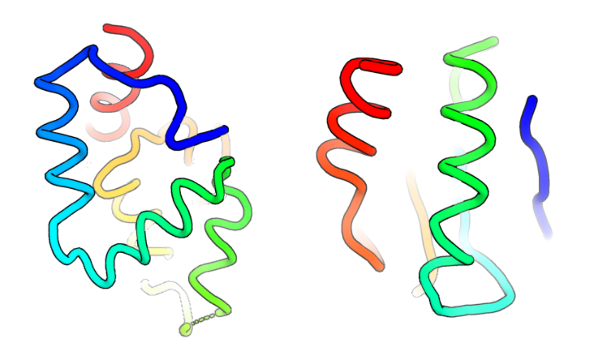
Figure 6: Two examples of protein backbone samples with incorrect left handed helices.

Appendix F Training details

ProtDiff uses 4 equivariant graph convolutional layers (EGCL) with 256 dimensions for node and edge embeddings. The training data was restricted to single chain proteins (monomers) found in PDB and lengths in the range [40, 128]. We additionally filtered out PDB with >5Å atomic resolution. This amounted to 4269 training examples. Training was performed using the Adam optimizer with hyperparameters learning_rate=1e-4, $\beta_{1}=0.9$, and $\beta_{2}=0.999$. We trained for 1,000,000 steps using batch size 16. We used a single Nvidia A100 GPU for approximately 24 hours. We implemented all models in PyTorch. We used the same linear noise schedule as Ho et al. (2020) where $\beta_{0}=0.0001$, $\beta_{T}=0.02$, and $T=1024$. We did not perform hyperparameter tuning.

Appendix G Additional metric details

Self-consistency algorithm. Section 5.1 described our self-consistency metrics for evaluating the designability of backbones generated with ProtDiff. Algorithm 4 makes explicit the procedure we use for computing these metrics.

Algorithm 4 Self-consistency calculation

1:$\mathbf{x}\in\mathbb{R}^{N,3}$

2:for $i\in 1,\dots,8$ do

3:     $s_{i}\leftarrow$ ProteinMPNN($\mathbf{x}$)

4:     $\hat{\mathbf{x}}_{i}\leftarrow$ AF2($s_{i}$)

5:end for

6:sc_tm $\leftarrow\max_{i\in 1,\dots,8}$TMscore$(\hat{\mathbf{x}}_{i},\mathbf{x})$

7:, sc_tm

Using dihedral angles to calculate helix chirality.

Natural proteins are chiral molecules that contain only right-handed alpha helices. However, because the underlying EGNN in our model is equivariant to reflection, it can produce samples with left-handed helices. While examining model samples, we additionally observed samples with both left and right-handed helices (Figure 6), even though in theory the EGNN should be able to detect and avoid the chiral mismatch. Left-handed helices are fundamentally invalid geometries in proteins and represent a trivial failure mode when calculating the self-consistency and other metrics. Samples with a mixture of left and right-handed helices are especially problematic because they cannot be corrected simply by reflecting the coordinates. As such, it is important to identify and separate samples with mixed chirality.

To detect chiralty, we compute the dihedral angle between four consecutive C-$\alpha$ atoms as a chiral metric to distinguish between the two helix chiralities. Algorithmically, for every C-$\alpha$ i, we calculate the dihedral between C-$\alpha$ i, i+1, i+2, and i+3. C-$\alpha$ i with dihedral angles between 0.6 and 1.2 radians are classified as right-handed helices, and angles between -1.2 and -0.6 are classified as left-handed helices, with everything else classified as non-helical. Because C-$\alpha$ atoms in native helices tend to form contiguous stretches longer than one residue in the primary sequence, helical stretches less than one amino acid were removed. This filtering is meant to help avoid accidentally counting the occasional isolated backbone geometry that falls into a helical bin as a true helix. Finally, for all C-$\alpha$ atoms i that are still categorized as part of a helix, the associated i+1, i+2 and i+3 C-$\alpha$ atoms are also counted as part of that helix.

Appendix H Additional experimental results

In this section, we describe additional results to complement the main text. We provide a description of the motif targets in Section 4, along with results of a scaffolding failure case in Section H.1. To understand the qualitative outcomes of scTM, we present additional results of backbone designs, their AF2 prediction, and most closely related PDB parent chain for different thresholds of scTM in Section H.2. We provide additional examples of latent interpolations in Section H.3. Finally, Section H.4 presents a structural clustering of unconditional backbone samples; this result provides further evidence of ProtDiff’s ability to generate diverse backbone structures.

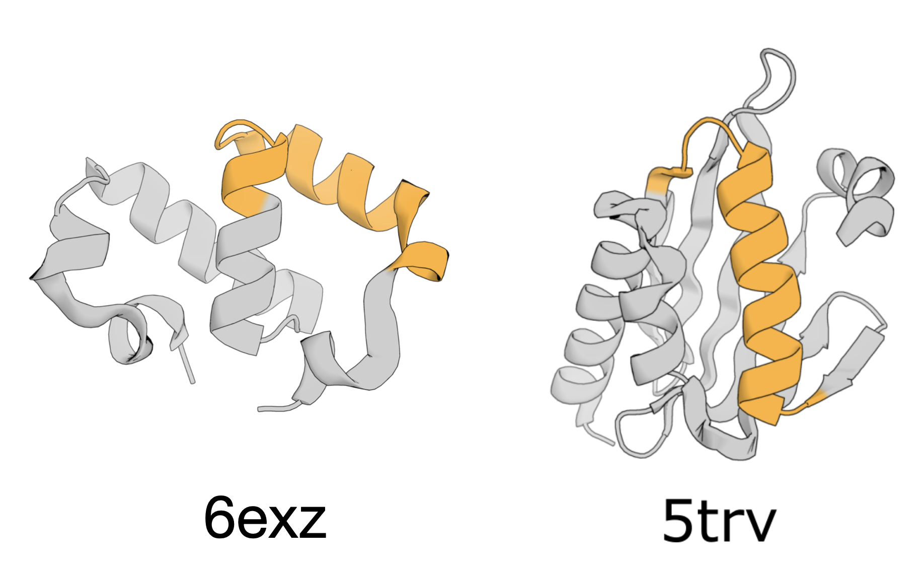
Figure 7: Structures used for motif-scaffolding test cases. Native structures (grey) and their motifs (orange) that were used for the motif-scaffolding task are shown.

H.1 Additional motif-scaffolding results

We here provide additional details of the motif-scaffolding experiments described in Section 5. Table 1 specifies the total lengths, motif sizes, and motif indices of our test cases. In Figure 7 we depict the structures of the native proteins (6exz and 5trv) from which the motifs examined quantitatively in the main text were extracted. Figure 8 analyzes commonly observed failure modes of ProtDiff backbone samples involving chain breaks, steric clashes, and incorrect chirality.

Figure 9 presents quantitative results on a harder inpainting target. In this case, the motif is defined as residues 163–181 of chain A of respiratory syncytial virus (RSV) protein (PDB ID: 5tpn). We attempted to scaffold this motif into a 62 residue protein, with the motif as residues 42–62. We chose this placement because previous work (Wang et al., 2022) identified a promising candidate scaffold with this motif placement. In contrast to the cases described in the main text, for which a suitable scaffold exists in the training set, SMCDiff and the other inpainting methods failed to identify scaffolds that recapitulated this motif to within a motif RMSD of 1 Å.

Table 1: Motif-scaffolding test case additional details.

Origin/ Protein	Total length	Motif size (residue range)
6exz	72	15 (30–44)
5trv	118	21 (42–62)
RSV (PDB-ID: 5tpn)	62	19 (16–34)
EF-hand (PDB-ID: 1PRW)	53	5 (0–4), 13 (31–43)

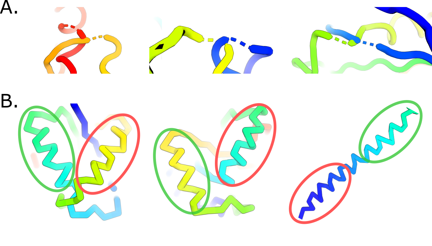
Figure 8: Failure modes in ProtDiff backbone samples. (A) Backbone clashes and chain breaks. The C-$\alpha$ atoms can be spaced further than the typical 3.8Å between neighbors, resulting in a chain break (dashed lines). Additionally, backbone segments can be too close to each other, resulting in obvious overlaps and clashes. (B) Backbones with a mixture of left (circled in red) and right (circled in green) handed helices. These chirality errors cannot be corrected simply by mirroring the sampled backbone.

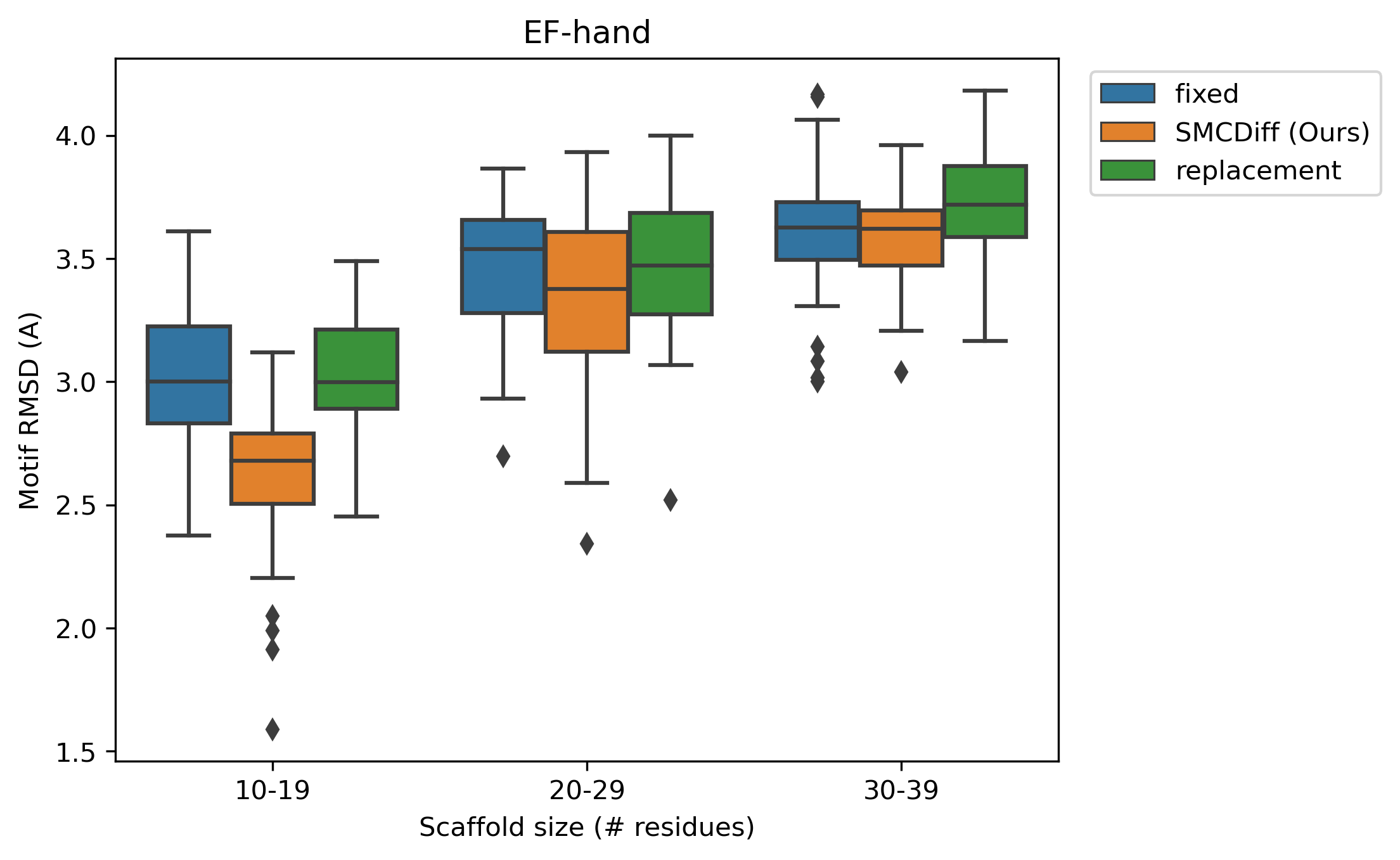
Figure 9: Additional inpainting results on a more challenging motif extracted from the respiratory syncytial virus (RSV) and EH-hand motif. The three inpainting methods are evaluated as described in Section 5.

H.2 Qualitative analysis of scTM in different ranges

In this section, we give intuition for backbone designs and AF2 predictions associated with different values of scTM to aid the interpretation of the scTM results provided in Section 5. Figure 10 examines a possible categorization of scTM in three ranges. The first two rows correspond to backbone designs that achieve scTM > 0.9. We see the backbone designs in the first column closely match the AF2 prediction in the second column. A closely related PDB example can be found when doing a similarity search of the highest PDB chain with the highest TM-score to the AF2 prediction. We showed in Figure 3B that scTM > 0.9 is indicative of a close structural match being found in PDB.

The middle two rows correspond to designs that achieve scTM $\sim$ 0.5. These are examples of backbone designs on the edge of what we deemed as designable (scTM > 0.5). In these cases, the AF2 prediction shares the same coarse shape as the backbone design but possibly with different secondary-structure ordering and composition. In the length 69 example, we see the closest PDB chain has a TM-score of only 0.65 to the AF2 prediction but roughly the same secondary-structure ordering as the backbone design. The length 100 sample is a similar case of AF2 producing a roughly similar shape to the backbone design, but has no matching monomer in PDB.

The final category of scTM < 0.25 reflects failure cases when scTM is low. The AF2 predictions in this case have many disordered regions and bear little structural similarity with the original backbone design. Similar PDB chains are not found. We expect that improved generative models of protein backbones would not produce any samples in this category.

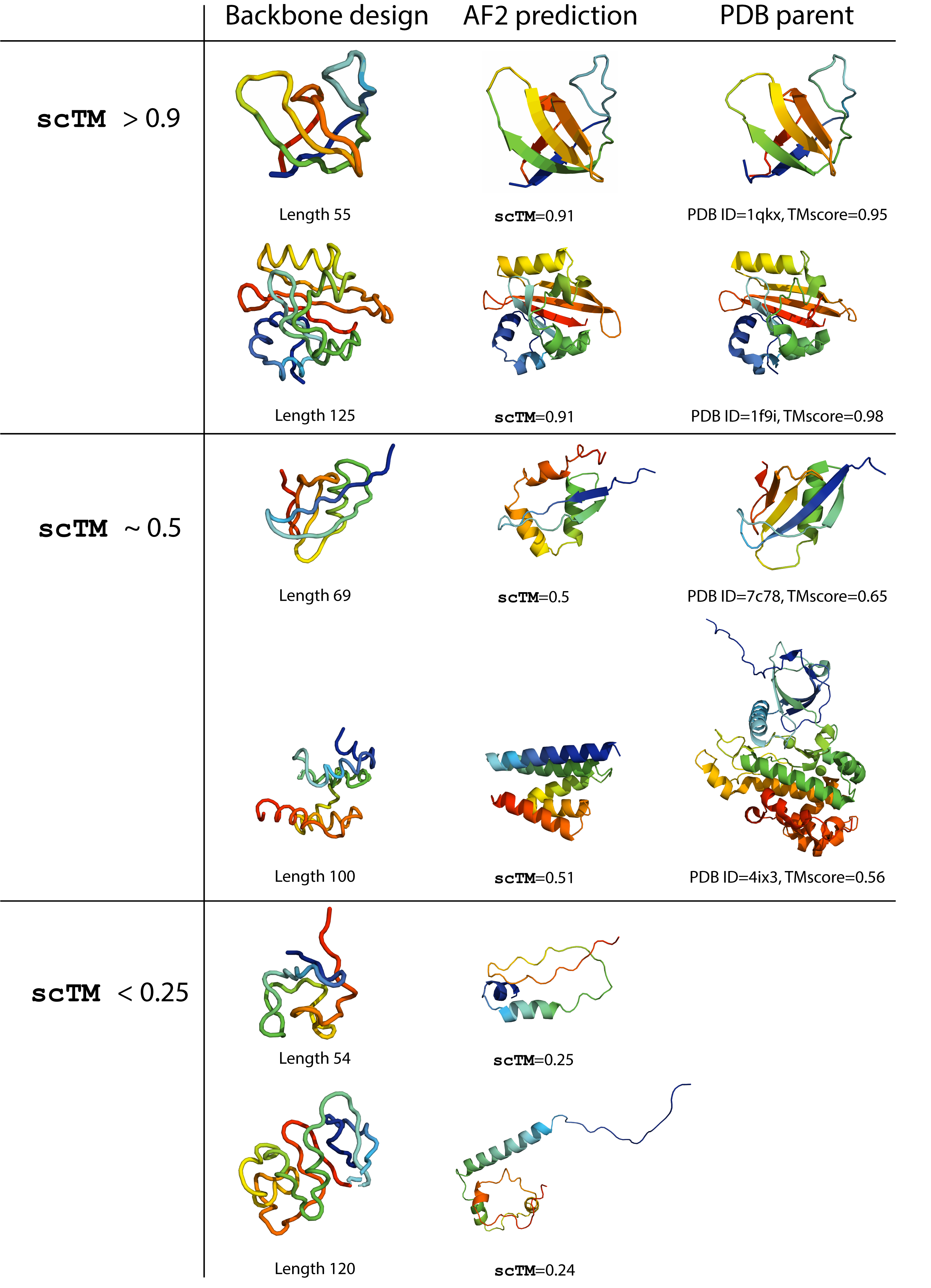
Figure 10: Qualitative analysis of unconditional backbone samples from ProtDiff. The first column displays backbone designs from ProtDiff and their sequence lengths. The second column displays the highest scTM scoring AF2 predictions from the ProteinMPNN sequences of the corresponding backbone design in the first column. The third column displays the closest PDB chain to the AF2 prediction in the second column with the PDB ID and TM-score written below. The third column is blank for the last two rows since no PDB match could be found. See Section H.2 for discussion.

H.3 Additional latent interpolation results

We here provide additional latent interpolations. Figures 11 and 12 depict interpolations for between model samples for lengths 89 and 63, respectively.

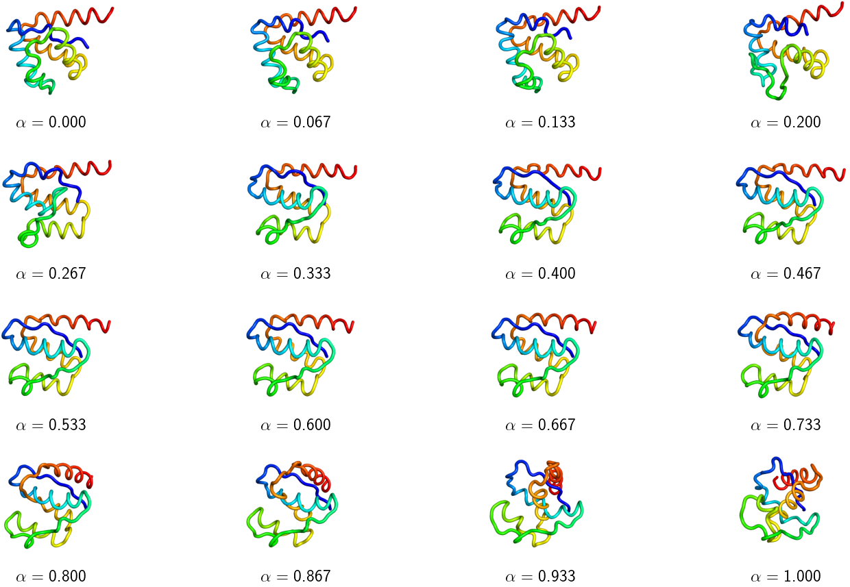
Figure 11: Latent interpolation of length 89 backbone sample from $\alpha=0$ to 1.

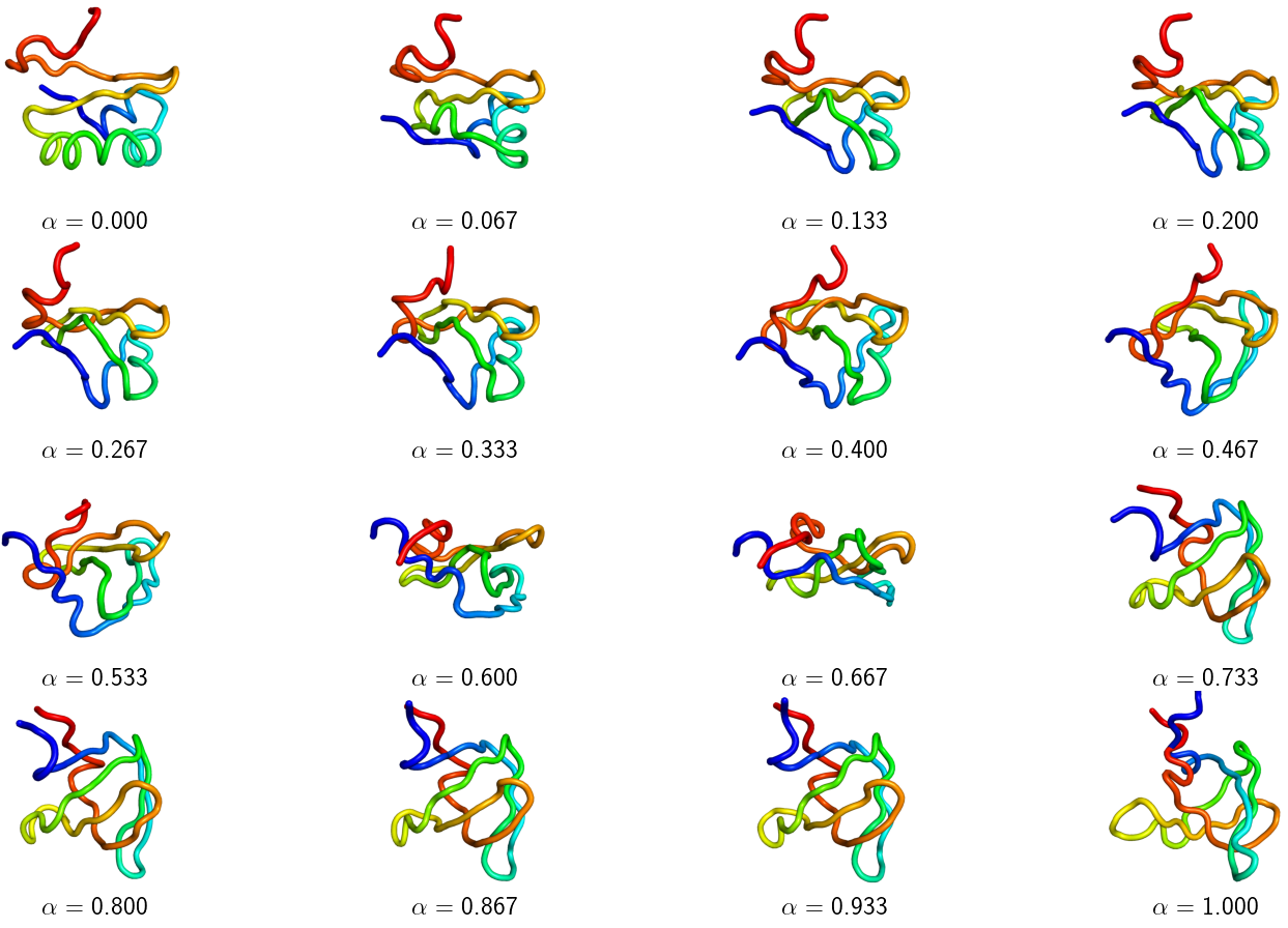
Figure 12: Latent interpolation of length 63 backbone sample from $\alpha=0$ to 1.

H.4 Structural clustering

All 92 samples with scTM > 0.5 were compared and clustered using MaxCluster Herbert & Sternberg (2008). Structures were compared in a sequence independent manner, using the TM-score of the maximal subset of paired residues. They were subsequently clustered using hierarchical clustering with average linkage, 1 - TM-score as the distance metric and a TM-score threshold of 0.5 (Figure 13 A).

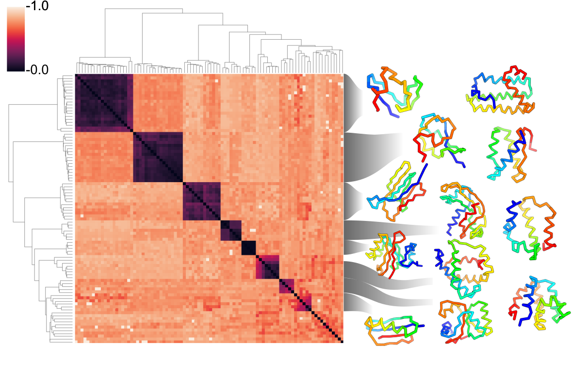
Figure 13: Clustering of self-consistent ProtDiff samples. The distance matrix is 1 - TM-score between pairs of samples, and ranges from 0 (exact matach) to 1 (no match). Dendrograms are from hierarchical clustering using the average distance metric. Designs on the right are cluster centroids. Gray lines connect larger clusters with more than one member to its centroid, while the remaining designs are from a random selection of the remaining single-sample clusters. Protein backbones are colored from blue at the N-terminus to red at the C-terminus.

Appendix I Applicability of SMCDiff beyond proteins: MNIST inpainting

Our goal in this section is to study the applicability of SMCDiff beyond motif-scaffolding, by applying it to inpainting on the MNIST digits dataset. We compare SMCDiff with the replacement method on the task of sampling the remaining half of MNIST digits. We first train DDPM with $\beta_{1}=10^{-4},\beta_{T}=0.2,T=1000$ using a small 8-layer CNN on MNIST with batch size 128 and ADAM optimizer for 100 epochs until it is able to generate reasonable MNIST samples (Figure 15). We then selected 3 random MNIST images and occluded the right half. The left half would then serve as the conditioning information to the diffusion model (Figure 15).

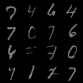
Figure 14: Unconditional MNIST samples.

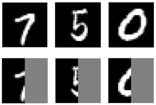
Figure 15: Full MNIST images and their occluded halves used for inpainting experiments.

For each occluded image, we fixed a single forward trajectory and sampled 16 images from each method: replacement method and SMCDiff with 16 or 64 particles $(K)$. Results are shown in Fig. 16. We observe the replacement method can sometimes produce coherent samples as a continuation of the conditioning information, but more often it attempts to produce incoherent digits. SMCDiff on the other hand tends to produce digits that compliment the conditioning information. For more difficult occlusions, such as 5 and 0, SMCDiff can still fail although increasing the number of particles ($K=64$) tends to produce samples that are more visually coherent.

It is important to note SMCDiff has additional computation overhead based on the number of particles. It can be more expensive than replacement method but result in higher quality samples. Investigating SMCDiff in more difficult datasets with improved architectures is a direction of future research.

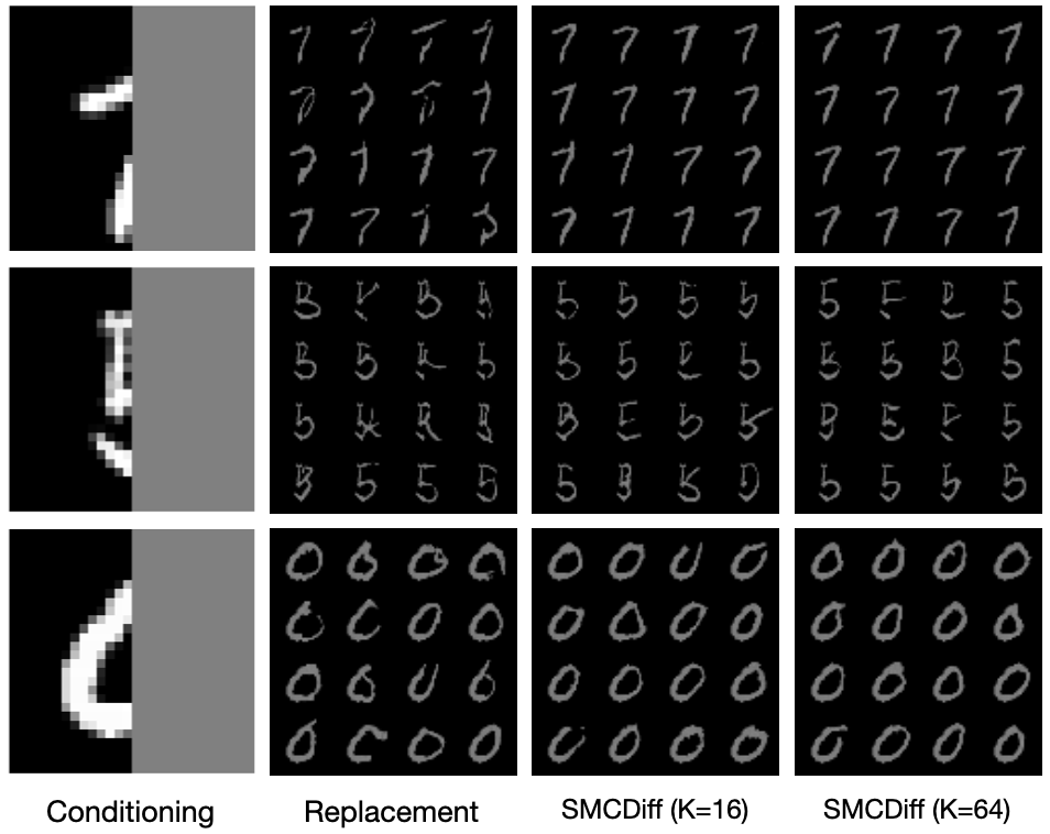
Figure 16: MNIST inpainting results for replacement and SMCDiff. See text for explanation.

References

- Anand & Achim (2022) Namrata Anand and Tudor Achim. Protein structure and sequence generation with equivariant denoising diffusion probabilistic models. arXiv preprint arXiv:2205.15019, 2022.
- Anand & Huang (2018) Namrata Anand and Possu Huang. Generative modeling for protein structures. In Advances in Neural Information Processing Systems, volume 31, 2018.
- Anfinsen (1973) Christian B Anfinsen. Principles that govern the folding of protein chains. Science, 181(4096):223–230, 1973.
- Anishchenko et al. (2021) Ivan Anishchenko, Samuel J Pellock, Tamuka M Chidyausiku, Theresa A Ramelot, Sergey Ovchinnikov, Jingzhou Hao, Khushboo Bafna, Christoffer Norn, Alex Kang, Asim K Bera, Frank DiMaio, Lauren Carter, Cameron M Chow, Gaetano T Montelione, and David Baker. De novo protein design by deep network hallucination. Nature, 600(7889):547–552, 2021.
- Batzner et al. (2022) Simon Batzner, Albert Musaelian, Lixin Sun, Mario Geiger, Jonathan P Mailoa, Mordechai Kornbluth, Nicola Molinari, Tess E Smidt, and Boris Kozinsky. E(3)-equivariant graph neural networks for data-efficient and accurate interatomic potentials. Nature Communications, 13, 2022.
- Bennett et al. (2022) Nathaniel Bennett, Brian Coventry, Inna Goreshnik, Buwei Huang, Aza Allen, Dionne Vafeados, Ying Po Peng, Justas Dauparas, Minkyung Baek, Lance Stewart, , Frank DiMaio, Steven De Munck, Savvas N. Savvides, and David Baker. Improving de novo protein binder design with deep learning. bioRxiv, 2022.
- Cao et al. (2022) Longxing Cao, Brian Coventry, Inna Goreshnik, Buwei Huang, Joon Sung Park, Kevin M Jude, Iva Marković, Rameshwar U Kadam, Koen H G Verschueren, Kenneth Verstraete, Scott Thomas Russell Walsh, Nathaniel Bennett, Ashish Phal, Aerin Yang, Lisa Kozodoy, Michelle DeWitt, Lora Picton, Lauren Miller, Eva-Maria Strauch, Nicholas D DeBouver, Allison Pires, Asim K Bera, Samer Halabiya, Bradley Hammerson, Wei Yang, Steffen Bernard, Lance Stewart, Ian A Wilson, Hannele Ruohola-Baker, Joseph Schlessinger, Sangwon Lee, Savvas N Savvides, K Christopher Garcia, and David Baker. Design of protein binding proteins from target structure alone. Nature, 605(7910):551–560, 2022.
- Chopin (2004) Nicolas Chopin. Central limit theorem for sequential Monte Carlo methods and its application to Bayesian inference. The Annals of Statistics, 32(6):2385–2411, 2004.