First optical identification of the SRG/eROSITA-detected supernova remnant  G 116.6$-$26.1   I. Preliminary results.

Abstract

The supernova remnant (SNR) candidate  G 116.6$-$26.1 is one of the few high Galactic latitude (|b| > 15^∘) remnants detected so far in several wavebands. It was discovered recently in the SRG/eROSITA all-sky X-ray survey and displays also a low-frequency weak radio signature. In this study, we report the first optical detection of  G 116.6$-$26.1 through deep, wide-field and higher resolution narrowband imaging in H$\upalpha$ , $[\text{S\,{ii}}]$ and $[\text{O\,{iii}}]$ light. The object exhibits two major and distinct filamentary emission structures in a partial shell-like formation. The optical filaments are found in excellent positional match with available X-ray, radio and UV maps, can be traced over a relatively long angular distance ($38\arcmin$ and $70\arcmin$) and appear unaffected by any strong interactions with the ambient interstellar medium. We also present a flux-calibrated, optical emission spectrum from a single location, with Balmer and several forbidden lines detected, indicative of emission from shock excitation in a typical evolved SNR. Confirmation of the most likely SNR nature of  G 116.6$-$26.1 is provided from the observed value of the line ratio [S ii] / H$\upalpha$ = $0.56\,\pm\,0.06$, which exceeds the widely accepted threshold 0.4, and is further strengthened by the positive outcome of several diagnostic tests for shock emission. Our results indicate an approximate shock velocity range 70–100 km s^-1 at the spectroscopically examined filament, which, when combined with the low emissivity in H$\upalpha$ and other emission lines, suggest that  G 116.6$-$26.1 is a SNR at a mature evolutionary stage.

1 Introduction

G 116.6$-$26.1 is a newly discovered Galactic supernova remnant (SNR) through soft X-ray imaging and spectra obtained with the Russian-German observatory SRG/eROSITA (Churazov et al., 2021). According to the X-ray observations, it is a faint and nearly circular object, with large angular size (about 4^∘ in diameter), located in high Galactic latitude. The morphological structure of the SNR candidate indicates a marginal brightening along the periphery (mostly in the southern and western portions) and signs of mild surface brightness enhancement at the innermost 20′of the object. Its soft X-ray imaging spectrum is dominated by O vii and O viii lines, similar to the surrounding background spectrum. Churazov et al. (2021) suggest that the supernova (SN) explosion took place in the halo of Milky Way, characterized by hot [$\sim$(1–2) $\times\,10^{6}\,K$] and low density (about $10^{-3}~{}cm^{-3}$) plasma.

They propose a relatively old remnant, originating from a thermonuclear explosion (SN Ia) that happened about 40 000 years ago, at an approximate distance of 3 kpc from us and about 1.3 kpc out of the Galactic disk. However, they do not reject the possibility of  G 116.6$-$26.1 being the result of a core collapse SN explosion. In favor of this scenario is the fact that probably the dust distribution in its neighborhood is affected by  G 116.6$-$26.1 , which would imply that this object is placed within 300 pc from us, resulting from a core collapse supernova explosion (SN II). In a very recent work, Churazov et al. (2022) report radio emission from  G 116.6$-$26.1 detected in the LOFAR Two-metre Sky Survey (LoTTS-DR2, Shimwell et al., 2022). It presents a faint, shell-like structure with good positional coincidence between the radio boundary and the X-ray limb, as presented in Churazov et al. (2021), while no optical counterparts have been reported until now.

In our Galaxy there are roughly 300 known SNRs (Green, 2019), with more than 90 per cent of them located within 5 degrees off the Galactic plane (Kothes et al., 2017), while $\sim$ 10 of the currently known remnants reside between latitudes 5 and 10 degrees. However, only a handful of these objects have been found in higher Galactic latitudes. Boumis et al. (2002) reported the discovery of optical filaments in Pegasus Constellation suggesting that are part of one (or more) SNRs. Its nature as such was also confirmed by Fesen et al. (2015) based on its morphology and its spectral characteristics. This is the G 70.0$-$21.5 remnant which was studied more recently also by Raymond et al. (2020), and it is believed to be the result of a type Ia SN. McCullough et al. (2002) discovered the Antlia SNR (or G 275.5$+$18.4), which was detected in H$\upalpha$ and X-rays. Later, Shinn et al. (2007) and Fesen et al. (2021) confirmed this identification, using GALEX FUV imagery and optical observations, respectively. Its progenitor is probably a B-type star (Shinn et al., 2007) and hence, it comes likely from a core collapse SN explosion.

Another high latitude SNR is the Hoinga or G 249.7$+$24.7 remnant discovered also in the X-ray SRG/eROSITA All-Sky Survey eRASS1 (Becker et al., 2021), which presents also radio, optical, and UV emission (Becker et al., 2021; Fesen et al., 2021). According to Becker et al. (2021), the fact that no pulsar has been associated with this remnant so far, in combination with its high latitude, indicate that it is probably the remnant of a type Ia SN explosion. The highest Galactic latitude SNR found yet, is G 354.0$-$33.5, observed in FUV, H$\upalpha$ , and radio wavelengths (Testori et al., 2008; Fesen et al., 2021). No evidence about its progenitor and/or the explosion type of this SNR is found.

In this work we report for the first time optical emission from  G 116.6$-$26.1 , based on both wide-field and higher resolution imaging as well as spectroscopic observations. The results seem to satisfy most of the criteria for the optical identification of SNRs. This, in combination with its spatial correlation with other wavelengths, enhances the belief of  G 116.6$-$26.1 being a new Galactic SNR. We also discuss the possible nature of its progenitor but we did not reach a secure conclusion. The structure of the paper is as follows: In Section 2 we describe the observations and the reduction of the imaging and spectroscopic data. In Section 3 we present the results of the aforementioned analysis. We quote available observations of  G 116.6$-$26.1 in other wavelengths and we explore their spatial correlation with the optical emission in Section 4. In Section 5 we discuss our results, while in Section 6 we summarise our conclusions.

2 Observations and Data Reduction

2.1 Imaging

2.1.1 Wide-field imagery

The first step in our search for possible optical line emission from the newly-discovered SNR  G 116.6$-$26.1 , was to perform wide-field imaging, since the reported angular diameter of the source in X-rays was estimated to be ${\sim}4\degr$ (Churazov et al., 2021). Such a capability is provided by the fast-optics (f/3.2), Schmidt-Cassegrain 0.3 m telescope (a Lichtenknecker Flat Field Camera, hereafter LFFC) at Skinakas Observatory in Crete, Greece. Coupled with a back-illuminated 2k $\times$ 2k CCD camera (by Andor Tech.), the telescope–instrument system offers a field of view (FoV) $100\arcmin\times 100\arcmin$ on the sky. The thermoelectric-cooled CCD sensor (operating temperature $-70\degr$ Celsius) shows negligible dark current, has pixel size 13.5 $\micron$ which corresponds to $2\aas@@fstack{\prime\prime}94$ on the celestial sphere.

This preliminary observing run aimed at the construction of a mosaic of partially overlapping images, wide enough to cover the reported X-ray extent of the source, in the light of H$\upalpha$ emission, in a $3\times 3$ frame pattern. The images were obtained with the LFFC telescope on 2021 September 1, 3–5 and October 7–8, through a narrow-band H$\upalpha$+$[\text{N\,{ii}}]$ filter. A red broadband continuum filter (SDSS$-$r’) was also used to provide images for subsequent subtraction of the background continuum and especially for the removal of the stellar component in the images in order to improve the visibility of very faint structures. Filter characteristics are given in Table 1. Each of the nine fields in the mosaic was observed for a total exposure time of 9000 s (15$\times$600 s) in H$\upalpha$+$[\text{N\,{ii}}]$  and 300 s (15$\times$20 s) through the continuum filter, respectively.

All nights were photometric and target fields ranged in airmass between 1.0 and 1.4 during observations. Multiple bias exposures and twilight flat frames of very high signal-to-noise (S/N) ratio were taken on a daily basis. We did not observe any spectrophotometric standard stars, because we were not planning to flux-calibrate our images taken with the LFFC 0.3-m telescope, serving the single purpose to visually examine the area for any H$\upalpha$ emission signature.

Table 1: The characteristics of the optical filters used in this research.

[b] Filter $\uplambda_{c}$^a FWHM Transm^b (Å) (Å) (%) H$\upalpha$+$[\text{N\,{ii}}]$  $\uplambda\uplambda$ 6548, 6584 Å 6582 82 99 $[\text{S\,{ii}}]$  $\uplambda\uplambda$ 6716, 6731 Å 6730 32 99 $[\text{O\,{iii}}]$  $\uplambda$ 5007 Å 5008 25 52 SDSS$-$r’ 6214 1290 96 Johnson/Bessell V 5380 980 88

• The central wavelength

• Peak filter transmittance

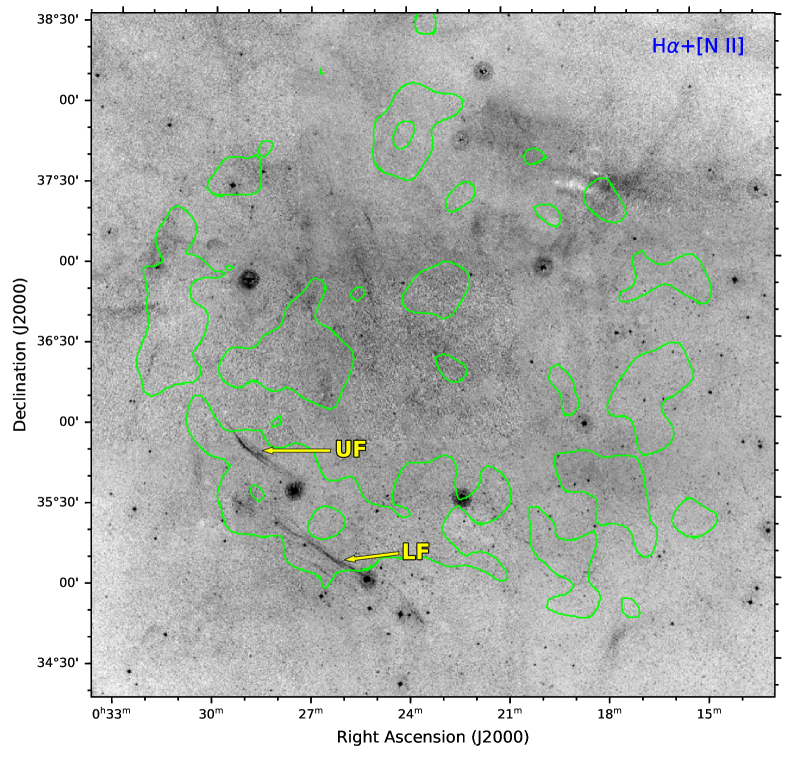
Figure 1: The continuum-subtracted 9-frame mosaic towards the SNR  G 116.6$-$26.1 in the light of H$\upalpha$+$[\text{N\,{ii}}]$ . Superposed contours (solid green lines) from the X-ray observations (Churazov et al., 2021) show the correlation between the optical filaments with the X-ray emission. Several artefacts in the form of dark round halo appear around bright stars which are not emission features but ghosts due to scattered light from internal reflections in the narrow-band filter.

The raw images were reduced using the IRAF software (Tody, 1986, 1993) procedures for bias subtraction and flat-field correction. Individual exposures of each of the 9 frames observed were registered to a reference image in the set and combined through a 3-sigma clipping average algorithm in order to remove cosmic rays and artificial satellite trails – a not so rare situation in modern era, especially in wide-field imaging. Astrometric calibration was performed with the aid of astrometry.net (Lang et al., 2010) web service, interfaced through AstroImageJ software (Collins et al., 2017). The next step was to use the narrow-band (H$\upalpha$+$[\text{N\,{ii}}]$ ) and continuum (SDSS-r’) images in order to subtract the sky background and eliminate as many field stars as possible to reduce crowding confusion, following a procedure described in Appendix A. Finally, the continuum-subtracted frames were assembled together into the final mosaic utilizing the Montage software with adjustment for smooth background levels between overlapping images. The final mosaic in H$\upalpha$+$[\text{N\,{ii}}]$ emission is shown in Fig. 1, where the presence of two major optical filaments is evident.

The detected sharp filaments shown in Fig. 1 were further investigated, using the LFFC telescope and H$\upalpha$+$[\text{N\,{ii}}]$ , $[\text{S\,{ii}}]$  and $[\text{O\,{iii}}]$ filters, on 2021 November 6 and 8, for a total exposure time of 3 h (18 images of 600 s each), 4 h (24$\times$600 s) and 3 h (9$\times$1200 s), through the respective filters. Multiple short exposures were also obtained in the respective continuum filters for background and starlight subtraction. The final background-subtracted images are shown in Fig. 2.

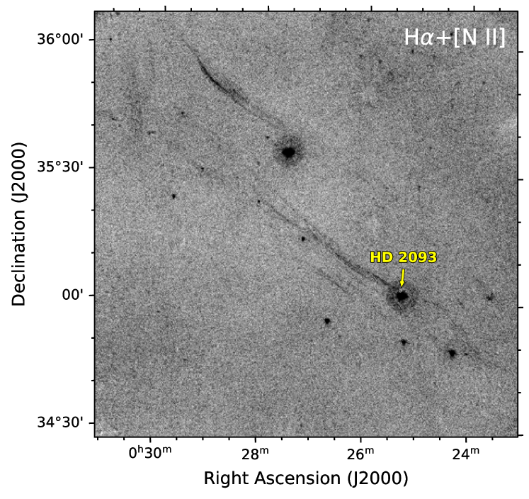
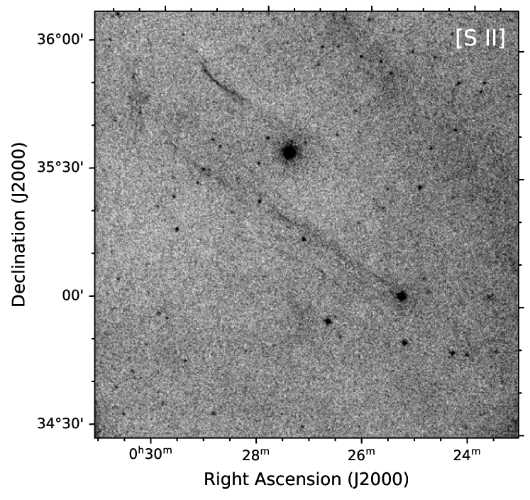
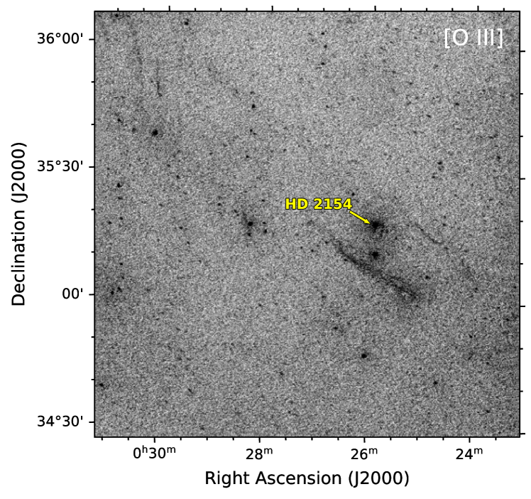
Figure 2: Low resolution negative images of the major optical filaments’ area, in H$\upalpha$+$[\text{N\,{ii}}]$   (top), $[\text{S\,{ii}}]$   (middle) and $[\text{O\,{iii}}]$   (bottom panel). Note that the dark spots and disc-like features scattered around the images, are residuals from imperfect subtraction of bright stars. These leftover artefacts in the bottom panel ($[\text{O\,{iii}}]$   filter) have no counterpart in the top and middle (red filters) images.

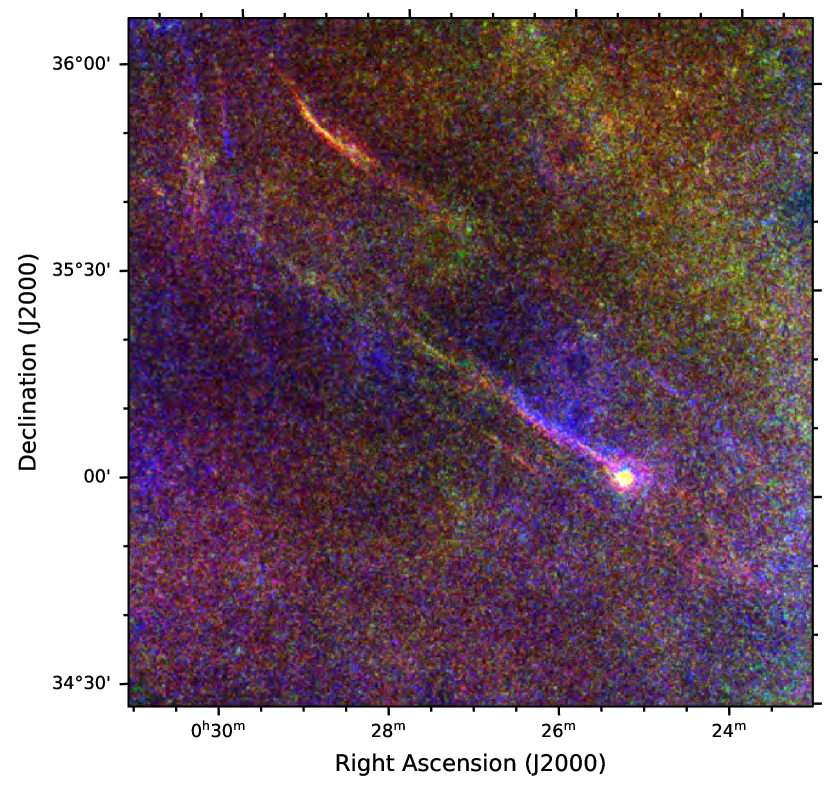
Figure 3: The area of the major optical filaments (Fig. 2) in H$\upalpha$+$[\text{N\,{ii}}]$ (red), $[\text{S\,{ii}}]$ (green) and $[\text{O\,{iii}}]$ (blue), to indicate the relative position of the emission in these three lines near the shock fronts.

2.1.2 Higher angular resolution imaging

Guided by the wide-field mosaic of the object’s H$\upalpha$+$[\text{N\,{ii}}]$  emission, additional images were taken of the upper and lower optical filaments at the south-eastern edge of the X-ray structure, using the 1.29 m (f/7.6) Ritchey–Chrétien telescope at Skinakas Observatory. Images were acquired with a 2048 $\times$ 2048 back-illuminated, deep-depletion CCD camera (Andor iKon-L) with pixel size 13.5 $\micron$. The system provided a 9$\aas@@fstack{\prime}$6 $\times 9\aas@@fstack{\prime}6$ FoV and image scale $0\aas@@fstack{\prime\prime}28$ per pixel. The narrow-band filters used are these in Table 1. Observations were held on 2021 July 15, September 10 and 12, October 4–5 and November 5, 7 and 11, under good seeing conditions ($0\aas@@fstack{\prime\prime}8$–$1\aas@@fstack{\prime\prime}2$) and high target elevation (airmass range 1.00–1.35). Images for a 3-frame mosaic were obtained in the H$\upalpha$+$[\text{N\,{ii}}]$  filter covering the brighter part of the upper filament (region UF in Fig. 1) with 9600 s (16$\times$600 s) total integration time for each frame. Another series of 16 $\times$ 600 s exposures in $[\text{S\,{ii}}]$ combined into a single-frame image of the brighter part of UF. The lower filament (designated region LF in Fig. 1) was also imaged – only with a partial filter coverage due to weather conditions – in H$\upalpha$+$[\text{N\,{ii}}]$  with 2 overlapping frames of 2 h total exposure time each ($12\times 600$ s).

Table 2: Spectroscopic observations log.

[b] RegionID Date Aperture center Aperture Exposures^a $\mathrm{X_{eff}}$^b R.A. (J2000) Dec (J2000) height (UT) (″) (s) UF 2021 Nov 3 $\mathrm{00^{h}29^{m}03\aas@@fstack{s}7}$ $\mathrm{+35^{d}51^{m}50^{s}}$ 22.5 $3\times 2400$ 1.035, 1.008, 1.002

• Number of individual exposures and common exposure time

• Effective airmass at each exposure. [$\mathrm{X_{eff}~{}=~{}\frac{1}{6}(X_{start}\,+\,4\,X_{mid}\,+\,X_{end})}$]

Table 3: Locations of fainter filaments detected in wide-field images, but not examined yet in detail.

[b] Filament center Approximate Appears Image R.A. (J2000) Dec (J2000) length (′) in figure filter $\mathrm{00^{h}25^{m}15^{s}}$ $\mathrm{+37^{d}15^{m}28^{s}}$ 6.7 Fig. 1 H$\upalpha$+$[\text{N\,{ii}}]$ $\mathrm{00^{h}25^{m}22^{s}}$ $\mathrm{+36^{d}52^{m}40^{s}}$ 18.5 Fig. 1 H$\upalpha$+$[\text{N\,{ii}}]$ $\mathrm{00^{h}24^{m}22^{s}}$ $\mathrm{+34^{d}57^{m}33^{s}}$ 7.7 Fig. 1 H$\upalpha$+$[\text{N\,{ii}}]$ $\mathrm{00^{h}24^{m}46^{s}}$ $\mathrm{+34^{d}55^{m}09^{s}}$ 6.9 Fig. 1 H$\upalpha$+$[\text{N\,{ii}}]$ $\mathrm{00^{h}24^{m}08^{s}}$ $\mathrm{+35^{d}01^{m}07^{s}}$ 2.6 Fig. 1 H$\upalpha$+$[\text{N\,{ii}}]$ $\mathrm{00^{h}30^{m}10^{s}}$ $\mathrm{+35^{d}51^{m}28^{s}}$ 8.6 Fig. 2 $[\text{O\,{iii}}]$ $\mathrm{00^{h}30^{m}40^{s}}$ $\mathrm{+35^{d}58^{m}48^{s}}$ 13.0 Fig. 2 $[\text{O\,{iii}}]$ $\mathrm{00^{h}25^{m}00^{s}}$ $\mathrm{+35^{d}18^{m}13^{s}}$ 12.6 Fig. 2 $[\text{O\,{iii}}]$ $\mathrm{00^{h}31^{m}38^{s}}$ $\mathrm{+37^{d}08^{m}18^{s}}$ 21.3 Fig. 12 Far UV

2.2 Spectrophotometry

Long-slit, low-resolution spectroscopic observations of the brightest part of the upper filament were made on 2021 November 3, using the 1.29 m telescope at Skinakas Observatory and a CCD camera of the same type and characteristics as in the higher resolution direct imaging, described in section 2.1.2. A 1302 grooves mm^-1 grating was used, blazed at 5500 Å, giving an average dispersion 0.94 Å pixel^-1 and spectral coverage 4820–6750 Å. The object spectra were taken with a slit of width 3$\aas@@fstack{\prime\prime}$9 (7$\aas@@fstack{\prime\prime}$3 slit used for the spectrophotometric standard stars), and usable length 14$\aas@@fstack{\prime}$5 – long enough to allow for background subtraction – always oriented along the North-South direction. Seeing varied between 1$\aas@@fstack{\prime\prime}$1 and 1$\aas@@fstack{\prime\prime}$5 under dark and photometric sky conditions.

Several zero-exposure (bias) images were collected each night along with two sets of exposures for flat-fielding. One set consisted of images taken with a quartz-lamp as light source inside the spectrograph and a diffuser in front of the slit, while the second set was a series of twilight sky exposures, in order to perform a slit illumination correction on the first set. Spectra were wavelength calibrated using a Ferrum-Helium-Neon-Argon comparison lamp and arc images were obtained after the end of each target exposure. Flux calibration of the spectral lines was achieved through exposures of the spectrophotometric standard stars HR718, HR1544, HR3454, HR7596, HR7950, HR9087 (Hamuy et al., 1992, 1994) and BD$+25{\degr}4655$, BD$+33\degr 2642$, G 191-B2B (Oke, 1990; Massey et al., 1988). Standards were observed every night in at least three different time slots, in groups of 4–6 stars for better airmass coverage.

One more set of images was acquired, necessary for the correction of optical distortion and curvature of the spectral features along the dispersion and spatial directions, which is quite noticeable in our long-slit spectra. A preselected nearby (angular distance ≲ 8°  from the observed target), very bright field star (visual magnitude 3.5–5.5) was positioned near one of the slit’s long-dimension ends and a series of spectral images was obtained, offseting the telescope in steps of $\approx 30\arcsec$ along the slit direction in-between exposures, until the other end of the slit was reached. This task is accomplished in less than 5 minutes, since typical exposure times for high signal-to-noise ratio individual spectra is 3–5 s. The images are added together during data reduction and give the equivalent of a multi-star spectrum, which, along with a comparison lamp exposure, can determine the geometric transformation needed to correct distortions in the two-dimensional science spectra.

Standard IRAF procedures (Valdes, 1992) were utilised for spectra reduction and extraction of calibrated line emission fluxes. The reduction steps include bias subtraction, flat-field correction, cosmic-ray removal using the software L. A. Cosmic (van Dokkum, 2001) and geometric rectification . Background estimation was performed in areas close to the spectral apertures and free of diffuse emission, selected with the guidance of the higher resolution images. Center coordinates and height of the aperture used in the spectra extraction, exposure date, integration times and effective airmasses are presented in Table 2.

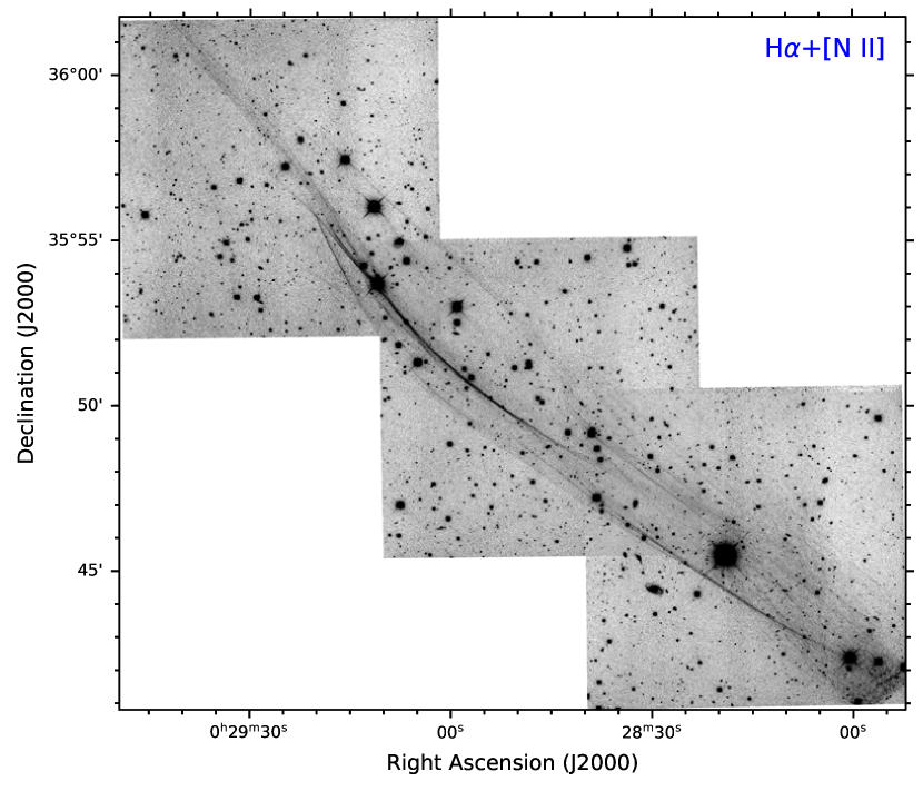
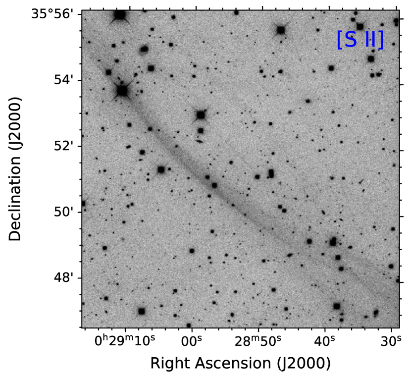
Figure 4: Higher angular resolution mosaic in H$\upalpha$+$[\text{N\,{ii}}]$   of the upper filament’s (UF) brighter segment. An orderly network of similarly aligned, hair-thin filaments of varying degree of curvature is prominent in this image.

Figure 5: The middle frame of the H$\upalpha$+$[\text{N\,{ii}}]$   mosaic in Fig. 5, as seen in $[\text{S\,{ii}}]$   emission light. Although images in both filters were obtained under the same seeing conditions, the filaments’ sharpness in $[\text{S\,{ii}}]$   is not comparable to that in H$\upalpha$ light.

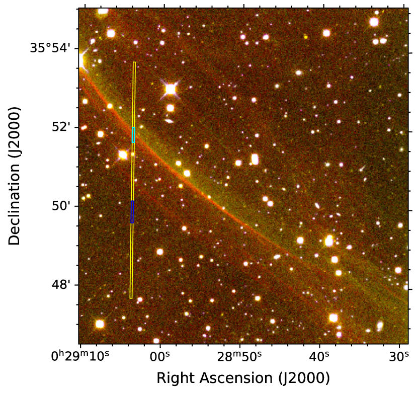
Figure 6: Uncalibrated bi-colour composite image of the area in Fig. 5 with H$\upalpha$+$[\text{N\,{ii}}]$   (red) and $[\text{S\,{ii}}]$   (green). The respective emissions at the brightest filament area seem to start at the same location (dark orange coloured post-shock shell), but the H$\upalpha$   intensity drops faster in the downstream direction compared to $[\text{S\,{ii}}]$ . The yellow, cyan and blue rectangles mark the locations of the slit, aperture for the extracted spectrum and sky area for background subtraction, respectively.

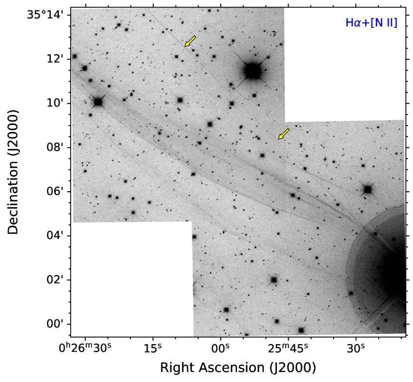
Figure 7: Two-frame mosaic in H$\upalpha$+$[\text{N\,{ii}}]$   of the brighter segments in region LF. Several thin filaments arranged along NE-SW direction, suggesting the presence of expanding emission shells, are mixed with fainter diffuse light, mostly in the downstream direction of the associated shock fronts. It should be noticed that the perfectly straight feature, running diagonally across the upper-right part of the image and marked with two yellow arrows, is neither an artificial satellite trail nor real thin filament. It is an optical artefact, a diffraction spike produced by copious light from the bright star HD 2093 (V =  7.36), just outside the lower right edge of the image.

3 Results

3.1 Direct Imaging

3.1.1 Wide-field coverage

The deep (total exposure time 22.5 h) H$\upalpha$+$[\text{N\,{ii}}]$  continuum-subtracted 9-frame mosaic of the area where candidate SNR  G 116.6$-$26.1 was discovered in X-rays, is shown in Fig. 1. The image center is at R.A. = $00^{\rm h}23^{\rm m}14^{\rm s}$, Dec. = $36^{\rm d}25^{\rm m}45^{\rm s}$ and has an angular length of $4\aas@@fstack{\circ}25$ on each side. Overlaid are X-ray contours from the SRG imaging observations (Churazov et al., 2021). The prominent set of two optical filaments (marked as UF – upper filament – and LF – lower filament) at the southeastern part of the X-ray image, running almost in parallel directions, are the major features seen in this wide-field image and there is very good positional match with the brightest contours of the X-ray map.

A few much fainter filaments are seen scattered, mostly at the eastern part of the SNR (near the left edge of the image, at Declination  $36\aas@@fstack{\circ}5$). Two more, very faint, straight and parallel to each other, filaments are located just north-east of the presumed center of the remnant [at (RA, Dec) $\simeq$ ($00^{\text{h}}25^{\text{m}}$, $37\degr 10\arcmin$)]. Another wider diffuse stripe is extending radially outwards the north-western corner of the image, which is also barely visible in the DSS red images and in the All-Sky H$\upalpha$ map with $6\arcmin$ resolution (Finkbeiner, 2003). This latter feature seems to be unrelated to the SNR emission. We did not investigate these fainter structures further, but will be included in our follow-up observations.

Fig. 2 presents a close-up (but still in low angular resolution) of the filaments, in H$\upalpha$+$[\text{N\,{ii}}]$ , $[\text{S\,{ii}}]$ and $[\text{O\,{iii}}]$ . UF is brighter in H$\upalpha$+$[\text{N\,{ii}}]$ and $[\text{S\,{ii}}]$ and marginally visible in $[\text{O\,{iii}}]$ . It appears slightly curved at its brighter portion, with the convex part facing towards the center of the SNR, and extends (in the red emission lines) for $\simeq\,38\arcmin$. On the other hand, in the $[\text{O\,{iii}}]$ light, UF appears fainter but seems it can be traced to a longer extend, getting a bit brighter towards its southwestern projected end, to the west of star HD 2154 (marked in bottom panel of Fig. 2).

The lower filament (LF) is more elongated compared to UF, with an estimated angular extend at least $70\arcmin$ (measured in the $[\text{S\,{ii}}]$ image), and despite its high angular length, it appears to be very straight, indicating it is part of a large-radius expanding shell and minimal interaction with any large-scale denser gaseous bodies (diffuse or molecular clouds). If we trace visually the lower filament, starting from its brighter projected end next to HD 2093 (see top panel in Fig. 2), its brightness remains more-or-less unchanged in all three emission lines, for about one third of its angular length, where a bifurcation occurs and $[\text{O\,{iii}}]$ emission is dimmed heavily. The northern branch, much fainter and sharper than the lower one, follows a remarkably straight path and is visible in both H$\upalpha$+$[\text{N\,{ii}}]$ and $[\text{S\,{ii}}]$ light. The lower branch appears brighter, a little wider and its continuity is interrupted for a short distance before its brightness weakens completely. South of the brighter part of LF and close to it (angular separation $\lesssim 6\arcmin$) a few short and fainter filaments are seen, running along in parallel to the major feature. Another network of curved filaments is visible – mostly in H$\upalpha$+$[\text{N\,{ii}}]$  – to the west of HD 2093 (top panel in Fig. 2).

We summarise in Table 3 the locations of fainter filamentary structures appearing in our wide-field imagery, which were not investigated any further in this preliminary report. The celestial coordinates of each filament’s estimated center along with their approximate angular length (in arcminutes) are listed there. In the last two columns of Table 3, the corresponding Figure number and the filter used in obtaining the associated image are given as well.

Figure 3 shows in colour representation the spatial distribution of the line emissions in H$\upalpha$+$[\text{N\,{ii}}]$ (red), $[\text{S\,{ii}}]$ (green) and $[\text{O\,{iii}}]$ (in blue hues). The shock fronts associated with the two filaments in this picture, are moving towards the lower left direction. In the UF, both H$\upalpha$+$[\text{N\,{ii}}]$ and $[\text{S\,{ii}}]$ contribute in brightness, with an apparent spatial precedence of the H$\upalpha$ emission. No appreciable light is seen in $[\text{O\,{iii}}]$ there. However, evidence for $[\text{O\,{iii}}]$ emission is provided both in the bottom frame of Fig. 2 and, more convincing, in the spectrum taken in region UF (see Sec. 3.2). Also, in the bright section of LF, the $[\text{O\,{iii}}]$ emission lags behind the H$\upalpha$ emitting front.

3.1.2 Higher angular resolution imaging

The two major filaments detected in our deep wide-field images can now be seen in greater detail in higher resolution H$\upalpha$+$[\text{N\,{ii}}]$ mosaics, in Figs. 5 and 7. A multitude of thin emission filaments exist, arranged almost in parallel directions with no apparent major distortion through interactions with the surrounding medium or signs of recent strong large-scale instabilities. Fig. 5 shows the $[\text{S\,{ii}}]$ emission at the region covered by the middle frame in the H$\upalpha$+$[\text{N\,{ii}}]$ mosaic in Fig. 5. Only the brighter filaments present in the H$\upalpha$ image are seen in $[\text{S\,{ii}}]$ , where the intensity scale-length in the emitting shell behind the shock front seems to be greater than that in H$\upalpha$ . This is clearly depicted in Fig. 7, where the H$\upalpha$ (red) emission brightness falls-off more quickly behind the shock than $[\text{S\,{ii}}]$ does.

At the brighter part of emission in the LF region a similar picture of several thin H$\upalpha$+$[\text{N\,{ii}}]$ filaments in close spacing arrangements is shown in Fig. 7. Near the southern frame’s lower edge, a short segment of the smaller companion filament is also visible (see Figs. 2 and 3).

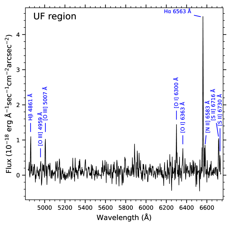
Figure 8: Emission line spectrum across filaments in region UF.

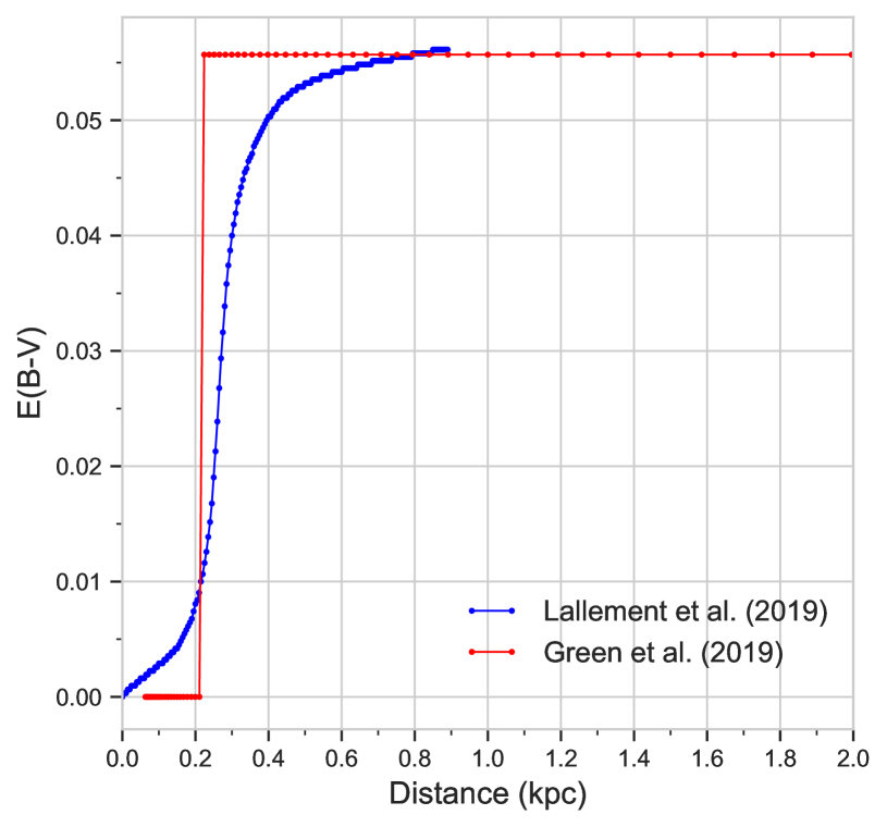
Figure 9: The colour excess $E(B-V)$ as a function of distance towards the region UF in  G 116.6$-$26.1 , according to the 3D dust maps of Lallement et al. (2019) and Green (2019).

[b]

Table 4: Normalised emission line fluxes from the extracted spectrum in the UF filament.

${\rm\uplambda}$ (Å), ID	Extinction function, $\text{f(}\uplambda)$a	F($\uplambda$)b	I($\uplambda$)c	S/Nd
4861 ${\rm H\upbeta}$	0.0000	100.0	100.0	8.1
4959 $[\text{O\,{iii}}]$	-0.0297	51.3	51.1	3.5
5007 $[\text{O\,{iii}}]$	-0.0446	123.6	122.6	7.7
6300 $[\text{O\,{i}}]$	-0.2835	151.3	143.6	8.1
6364 $[\text{O\,{i}}]$	-0.2924	55.2	52.3	6.1
6563 ${\rm H\upalpha}$	-0.3224	382.1	360.0	39.2
6583 $[\text{N\,{ii}}]$	-0.3256	75.9	71.4	12.1
6716 $[\text{S\,{ii}}]$	-0.3458	138.5	129.9	8.7
6731 $[\text{S\,{ii}}]$	-0.3479	75.5	70.8	5.2
Observed ${\rm F(H\upbeta})$e		$7.75\,\pm\,0.9$
${\rm c(H\upbeta)}$f		$0.080\,\pm\,0.17$
${E(B-V)}$g		$0.054\,\pm\,0.12$

• Derredening function according to Fitzpatrick et al. (2019) extinction law and extinction ratio R(V) =  3.1. See Appendix B for details.

• Observed line flux normalised to ${\rm H\upbeta=100}$.

• Intrinsic flux ratio, i.e. flux relative to ${\rm H\upbeta=100}$ corrected for interstellar extinction.

• Signal to noise ratio (S/N) for the observed flux ratio. Error contribution from the ${\rm H\upbeta}$ flux is not included in the noise term.

• In units of $10^{-18}$ erg Å^-1 s^-1 cm^-2 arcsec^-2.

• Logarithmic ${\rm H\upbeta}$ extinction coefficient: ${\rm c(H\upbeta)=log[(H\upbeta)_{intrinsic}/(H\upbeta)_{observed}]}$.

• $B-V$ colour excess.

Table 5: Major dereddened flux ratios of the UF spectrum.

Line ratio	Value
[S ii] $\uplambda\uplambda$ 6716, 6731 / H$\upalpha$	$0.56\,\pm\,0.06$
$[\text{N\,{ii}}]$ $\uplambda$ 6583 / ${\rm H\upalpha}$	$0.20\,\pm\,0.02$
$[\text{O\,{iii}}]$ $\uplambda$ 5007 / ${\rm H\upbeta}$	$1.23\,\pm\,0.22$
$[\text{O\,{i}}]$ $\uplambda$ 6300 / ${\rm H\upalpha}$	$0.40\,\pm\,0.05$
${\rm I(6716)/I(6731)}$	$1.83\,\pm\,0.41$
$[\text{N\,{ii}}]$ $\uplambda$ 6583 / [S ii] $\uplambda\uplambda$ 6716, 6731	$0.36\,\pm\,0.05$

3.2 Optical spectroscopy

A low resolution, long-slit spectrum was acquired at a bright filament position in region UF (see Table 2) with the Skinakas spectrograph, mount on the 1.29 m RC telescope. Individual exposures on the target were aligned spatially (via spectra of stars in the slit) and along the dispersion direction (using sky emission lines), corrected for atmospheric extinction and the 2D images were averaged. Extraction aperture was selected to sample relatively brighter region across the filaments and background was estimated from emission free regions, at the closest possible distance from the extraction aperture. The exact location of the slit aperture used for object and background extraction is shown overlaid in Fig. 7. Line fluxes were measured fitting Gaussians over a linear local background estimate.

The resulting flux-calibrated spectrum is presented in Fig. 8. Correction of the line emission fluxes for attenuation effects due to interstellar extinction was performed with the Balmer decrement method. We used the Fitzpatrick et al. (2019) extinction law corresponding to the mean galactic ratio of total-to-selective extinction R(V) = 3.1, and details on the derivation of the extinction function are given in Appendix B.

The usual practice in performing flux dereddening is to select, as a first step, a value for the intrinsic Balmer decrement $\text{I(H}\upalpha)/\text{I(H}\upbeta)$, appropriate for the type of gaseous nebula studied. In the SNR case, the adopted values are either $\text{I(H}\upalpha)/\text{I(H}\upbeta)$ = 2.86 – the theoretical Case B recombination (nebula optically thick to the Lyman series photons) – seen mostly in H ii regions, or $\text{I(H}\upalpha)/\text{I(H}\upbeta)$ = 3.0 when conditions favour the likelihood of significant collisional excitation of hydrogen in the post-shock region (e.g. Raymond et al., 2020; Fesen et al., 2021). Indeed, models with self-consistent treatment of the precursor ionization for a wide range of shock velocities (v${}_{s}=$ 10–1500 km $s^{-1}$) indicate that the intensity ratio $\text{I(H}\upalpha)/\text{I(H}\upbeta)$ exceeds always the Case B value 2.86 and varies between $\sim$ 3.0–5.0. In lower-velocity shocks the H$\upalpha$ /H$\upbeta$ flux ratio is strongly enhanced by collisional excitation in the postshock gas (Raymond, 1979; Chevalier et al., 1980; Cox & Raymond, 1985; Hartigan et al., 1987; Sutherland & Dopita, 2017; Dopita & Sutherland, 2017). The derived value of the extinction $A(V)$ and colour excess $E(B-V)$ are then compared to estimates from independent sources.

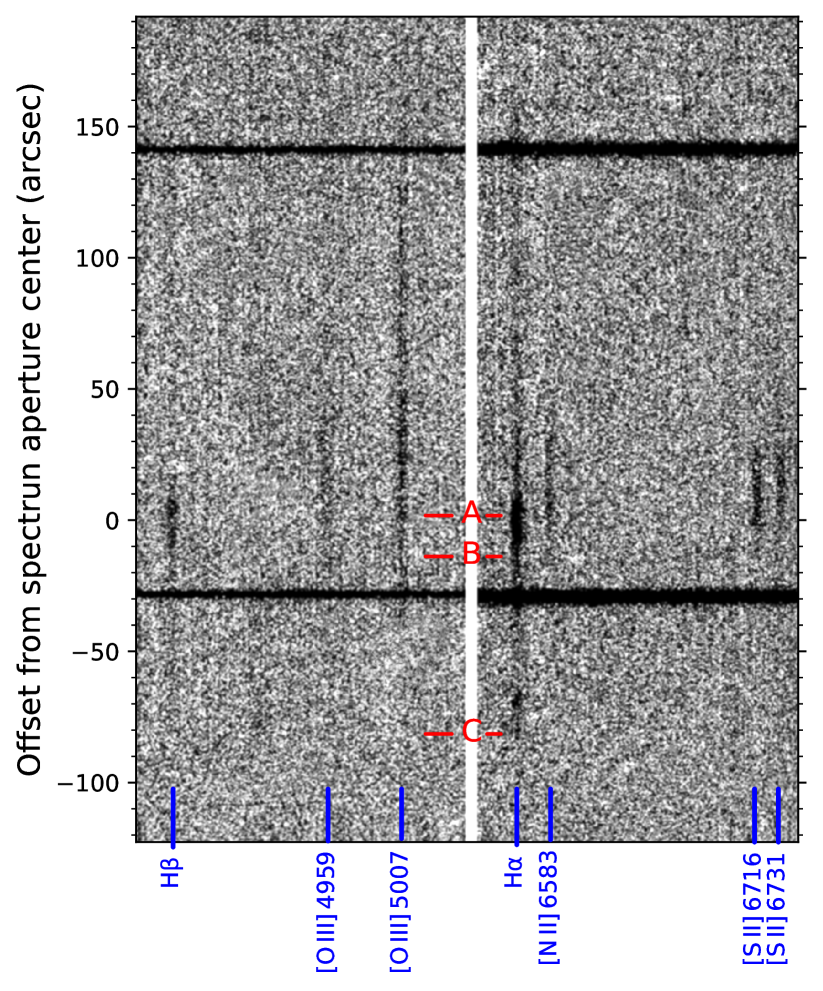
Figure 10: Part of the long slit spectral image in region UF, showing the spatial correlation of major emission lines identified with labels at the bottom. The [O i] $\uplambda\uplambda 6300,6364$ lines are not included for reasons explained in the text. The vertical axis scale corresponds to the angular offset from the extraction aperture center (value 0) across the slit aligned along the N-S direction. Positive numbers correlate with northern displacements (post-shock region). The white vertical stripe separates the bluer (left) from the redder wavelengths and the two horizontal black bands running across the image width are spectra of stars aligned in the slit. Letters and short horizontal line segments in red indicate the location of filaments discussed in the text.

In this study, we decided to take a different approach and adopt a value for the Balmer decrement $\text{I(H}\upalpha)/\text{I(H}\upbeta)$ such that the resulting colour excess $E(B-V)$ agrees with the extinctions predicted by the 3D dust maps of Lallement et al. (2019) and Green (2019) in the direction of  G 116.6$-$26.1 . Both dust maps show a gradual increase of $E(B-V)$ to 0.055 at a distance $\sim 400$ pc, and remains flat to larger distances (see Fig. 9). This requirement leads to intrinsic Balmer decrement $\text{I(H}\upalpha)/\text{I(H}\upbeta)\,=\,3.6$, which corresponds to shock velocity range 75 $\lesssim$  (v_s / km s^-1) $\lesssim$ 120, as predicted by relevant models (see Sutherland & Dopita, 2017, fig. 18). It should be emphasized that the emission line ratios, useful in diagnostic criteria, are insensitive to the reddening parameters used, because by construction, they correspond to wavelengths close to each other, and thus line fluxes are almost equally affected by interstellar extinction.

Dereddened fluxes were calculated with the aid of Equations 9 and B, derived in Appendix B, and the colour excess applying Eq. B. Listed in Table 5 are the measured $\text{F}(\uplambda)$ and extinction corrected $\text{I}(\uplambda)$ fluxes, normalised to $\text{F(H}\upbeta)=100$ and $\text{I(H}\upbeta)=100$, respectively, as well as the logarithmic H$\upbeta$  extinction coefficient c(H$\upbeta$) and colour excess $E(B-V)$. The S/N values given in the last column of Table 5 do not include calibration errors, estimated to be less than 15 per cent, neither the contribution of the normalising H$\upbeta$  flux error. It should be also noticed the relatively high uncertainty in the interstellar extinction related values of c(H$\upbeta$) and $E(B-V)$, reflecting the high relative error in the H$\upbeta$ flux (8 per cent).

The spectrum of a filament in region UF presents clear evidence that the associated emission results from shock-heated gas, commonly seen in SNRs. The widely accepted criterion supporting this is the observed value of [S ii] / H$\upalpha$ = 0.56 $\pm$ 0.06, exceeding the threshold 0.4, which separates SNRs from H ii regions (Dodorico, 1978; Blair et al., 1981; Dopita et al., 1984; Fesen et al., 1985). Another sensitive shock emission test is provided through the [O i] / H$\upbeta$ ratio, found to be 0.40 at a significance level of $8\,\upsigma$. This line ratio does not exceed 0.1 in H ii regions while higher values are associated with emission from shock heated interstellar nebulosities, like the shocks in SNRs (e.g. Fesen et al., 1985; Kopsacheili et al., 2020).

The electron density-sensitive [S ii] ratio $\uplambda\uplambda$ 6716 / 6731 was found to be above the low-density limit, [0.436 $\leq$ 6716 / 6731 $\leq$ 1.434 (Proxauf et al., 2014; Osterbrock & Ferland, 2006)], but with a high uncertainty, I(6716) / I(6731) = $1.83\,\pm\,0.41$. Therefore, we can not estimate the electron density (in the zone where S⁺ recombines) with confidence but only state that n${}_{e}\,\lesssim 100$ cm^-3.

Another remarkable property revealed from the spectrum sampled in the UF filament is its low brightness. The measured flux F(H$\upalpha$) = (2.96 $\pm$ 0.08)  $\times 10^{-17}$ erg Å^-1 s^-1 cm^-2 arcsec^-2 is 1–3 orders of magnitude fainter than most of the Galactic SNRs observed in the optical (e.g. Alikakos et al., 2012; Boumis et al., 2005, 2008; Boumis et al., 2009; Mavromatakis et al., 2002; Mavromatakis et al., 2005; Mavromatakis et al., 2009; How et al., 2018).

3.3 Post-shock emission morphology

Figure 10 presents two sections of the negative, background-subtracted 2D spectral image in the region UF filaments. The spatial variation of emitted fluxes in several emission lines – marked at the bottom of the picture – is shown with respect to angular distance from the aperture center (at value 0) used for the spectrum extraction, along the slit, aligned in the N-S direction. Positive numbers on the left axis scale correspond to northern displacements (down-stream direction relative to the shock fronts). Marked also with letters and short horizontal red line segments are the locations of filaments, as identified from the higher resolution H$\upalpha$+$[\text{N\,{ii}}]$ image in Fig. 5. It should be mentioned that only light emitted from filaments A and B is included in the aperture of the extracted spectrum in Fig. 8.

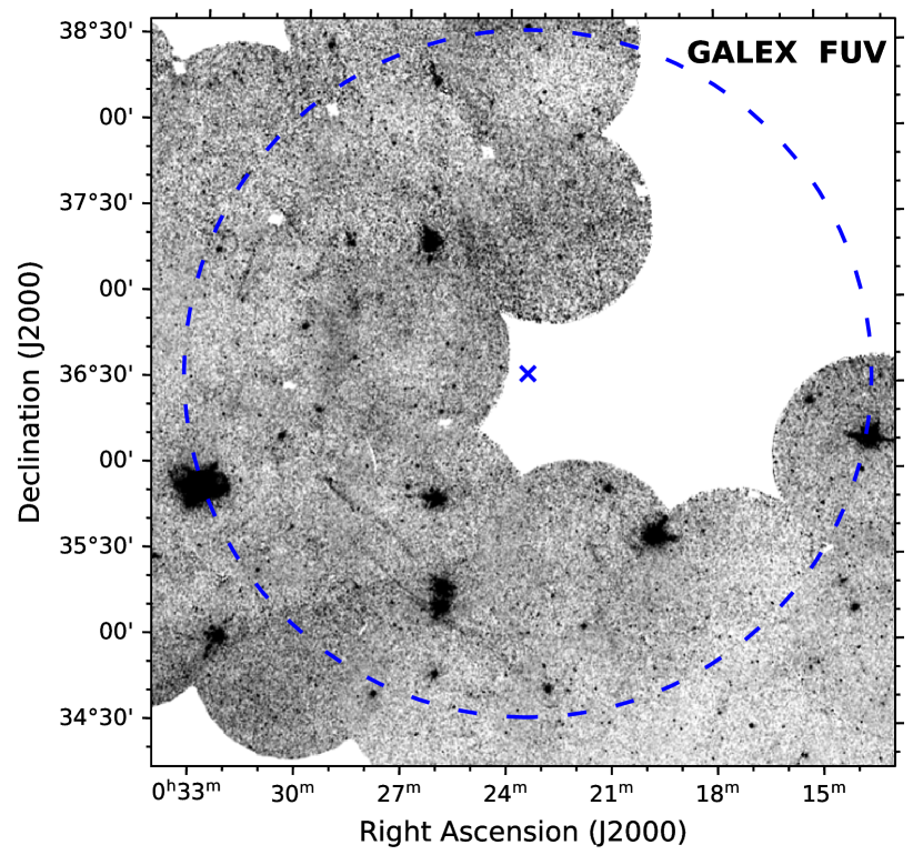
Figure 11: GALEX-FUV image covering the area of  G 116.6$-$26.1 . The dashed blue circle defines the X-ray extend of the supernova remnant and the $\times$ symbol marks its center. The filamentary structures near the center of the south-eastern quadrant are located at the same position as in our H$\upalpha$+$[\text{N\,{ii}}]$ wide-field image in Fig.1.

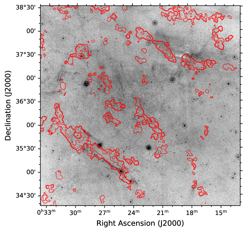
Figure 12: Contours of radio emission in 120–168 MHz from LOFAR LoTSS DR2 images superposed on our continuum-subtracted wide field H$\upalpha$+$[\text{N\,{ii}}]$ image (Fig. 1). The coincidence of the major optical filaments with the enhanced radio brightness at the south-eastern edge is evident. Contours shown correspond to 1, 5 and 20 $\upmu$Jy beam^-1 levels of flux density in the radio data.

Despite the fact that [O i] $\uplambda\uplambda$ 6300,6364 emission lines are equally important in SNRs, we do not include the corresponding part in the 2D spectral image in Fig. 10. The reason is that these lines are also quite strong in the night sky spectrum and the background subtraction procedure does not provide a smooth result at the positions of the [O i] lines. Thus, in our low resolution spectroscopy, the absence of considerable velocity component in the SNR [O i] lines to produce sufficient Doppler shift, combined with the intrinsic faintness of the nebular emission (even in H$\upalpha$) yield relatively ‘noisy’ background-subtracted [O i] lines and result in a rather confusing picture.

Starting from the most southern filament C, this appears as a diffuse and very faint feature which is seen in the spectrum to emit basically H$\upalpha$ light and just a weak hint of H$\upbeta$ emission at nearly the noise level. Filaments A and B are projected close to each other, at an angular distance $\simeq 19\arcsec$. H$\upalpha$ emission starts ahead of the brightest parts of the filaments, along with some H$\upbeta$ and weak $[\text{O\,{iii}}]$  light, but no detection of emission from other low-excitation lines, such as [$\text{N\,{ii}}]$ $\uplambda\uplambda$ 6548,6583 and [S ii] $\uplambda\uplambda$ 6716,6731. The H$\upalpha$ intensity increases for a short distance and then slowly decreases over a relatively long interval ($\simeq\,100\arcsec$) before it fades completely. The second Balmer line (H$\upbeta$ ) follows a similar variation but becomes undetectable much earlier, shortly after its peak. Heavier ions, like N⁺  and S⁺, start emitting further downstream, behind the location of maximum H$\upalpha$ emission and for a short angular distance, roughly 30$\arcsec$.

In contrast, in the line $[\text{O\,{iii}}]$  $\uplambda$ 5007, emission can be traced for much longer distance, seen almost as far as the H$\upalpha$ light, but in low intensity. The detected $[\text{O\,{iii}}]$  emission in the post-shock region suggests a lower limit on the shock velocity v_s of about 70 km s^-1, while its low brightness implies that this value is not expected to be much higher than 90 km s^-1. These limits were found from the diagram in fig. 6 of Dopita & Sutherland (2017), using the measured line ratio log([O iii] $\uplambda$5007 / H$\upbeta$) = 0.09 $\pm$ 0.08 (see Table 5), and come to agreement with the implied shock velocity range through our earlier choice for the intrinsic Balmer decrement $\text{I(H}\upalpha)/\text{I(H}\upbeta)$, in the extinction correction procedure of the spectral line fluxes.

One additional advantage of using the line ratio [O iii] $\uplambda$5007 / H$\upbeta$ to constrain the shock velocity range is the very weak dependency of its value on density (Dopita & Sutherland, 2017). However, the lower limit on the shock velocity implied by the detection of [O iii] $\uplambda$5007  emission, is based on the assumption that O⁺⁺ ions are not present in the preshock gas, or else [O iii] emission lines can be produced in much slower shocks (Raymond, 1979). This latter situation cannot be excluded from our spectrum, since the preshock area is projected on the postshock region of another, much weaker shock-front, leading ahead of the brighter filament in this region.

A similar structure behind relatively slow shocks (v${}_{s}\lesssim$ 150 km s^-1) was found in optical spectroscopic investigations of other high galactic latitude SNRs, such as G 70.0$-$21.5 (Raymond et al., 2020), G 107.0$+$9.0 (Fesen et al., 2020) and in the Hoinga or G 249.5$+$24.5 SNR (Becker et al., 2021; Fesen et al., 2021). The coexistence of radiative and Balmer dominated shock fronts in these supernova remnants indicate variable velocities of expansion in filamentary structures at different locations of the remnants.

4 Observations at other wavelengths

4.1 X-rays

G 116.6$-$26.1 has been discovered in X-rays, through the SRG/eROSITA all-sky survey (Churazov et al., 2021), as a faint, very extended circular feature with a total 0.3–2 keV flux of about 3 $\times$ 10^-11 erg s^-1cm^-2 distributed over a projected area $\sim$ 11.8 deg². The soft X-ray image depicts the circular source with a slightly brightened rim, especially across the south-eastern edge and two compact knots (seen in the smoothed version of the X-ray image), one near the western ridge and the other close to the center of the object. Comparing the location of the two major optical filaments in Fig. 1 with the overlaid X-ray brightness contours, there seems to be a clear correlation of the optical features with one of the stronger X-ray emission parts of the remnant at south-west. A second area of enhanced X-ray brightness appears at the northern part of the remnant, where no optical counterpart was found thus far.

4.2 Ultraviolet data

Our search for ultraviolet counterpart to the optical filaments has been performed with the publicly available imagery of the Galaxy Evolution Explorer (GALEX) space telescope All-Sky Imaging survey (AIS), described in detail in Morrissey et al. (2007). The GALEX archival database contains far-UV (FUV, $\mathrm{\uplambda_{eff}\sim}$1528 Å, 1344–1786 Å) and near-UV (NUV, $\mathrm{\uplambda_{eff}\sim}$2310 Å, 1771–2831 Å) direct imaging and grism spectra.

Figure 12 presents the GALEX FUV intensity mapping of the SNR  G 116.6$-$26.1 area, enclosed in a dashed circle of radius 2^∘ determined from the X-ray discovery image. Evidently, the two parallel filaments present in the middle of the south-east quadrant in the FUV image, are registered at exactly the same location as in our optical image and have similar lengths. These filaments are also visible in the GALEX NUV image, although they appear quite fainter. The NUV image is not shown here because the numerous artefacts in it produce a rather confusing picture of the field. One more, much shorter but quite sharp filament can be seen near the eastern edge of the FUV image (Declination $37\degr 00\arcmin$–$37\degr 20\arcmin$), which is not clearly seen in our wide field H$\upalpha$+$[\text{N\,{ii}}]$ image, a point that will be re-examined during our follow-up observations.

4.3 Observations in Radio frequencies

We have also used archival data from the large scale survey GALFA-H i DR2 of Galactic neutral hydrogen in the 21 cm radio line (Peek et al., 2018), to search for possible radio emission in the supernova remnant area, partially included in declination within the field covered by the survey. The available data cover a velocity range from $-$188.4 to $+$188.4 km s^-1 with respect to the Local Standard of Rest, in slices with spacing 0.184 km s^-1. Several features are present in the area but no association with the visible filaments or the overall X-ray contour morphology could be established.

However, Churazov et al. (2022) reported recently detection of extremely faint radio emission towards  G 116.6$-$26.1 from the LOFAR Two-metre Sky Survey (LoTSS) DR2 images (Shimwell et al., 2022). These data include 120–168 MHz images, mapping 27 per cent of the northern sky in low frequency at 6$\arcsec$ resolution, offering full bandwidth Stokes I total intensity maps, linear polarization image cubes and circular polarization continuum images.

In order to examine the spatial correlation between the optical filaments with the radio emission, we constructed a mosaic from archival LOFAR images of the  G 116.6$-$26.1 projected area of size $5^{\circ}\times 5^{\circ}$, partially removed point-like radio sources and created a network of contours at flux density levels 1, 5 and 20 $\upmu$Jy beam^-1. Fig. 12 shows these radio contours overlaid on our continuum subtracted H$\upalpha$+$[\text{N\,{ii}}]$ wide field image (in Fig. 1). The major parts of the radio emission structure consist of two elongated linear features, almost parallel to each other and running along the NE to SW direction, located at the diagonals of the SE and NW quadrants of the image. These linear structures’ northern ends are connected by a faint circular arc, completing a figure reminiscent of a horse-shoe. The eastern branch of this feature is the brightest and coincides with the location of the two major optical filaments, as seen in Fig. 12.

The north-western segment may indicate the location for another possible optical feature. Close inspection of our H$\upalpha$+$[\text{N\,{ii}}]$ image reveals the presence of some diffuse and extended optical emission, displaced towards the NW relative to the radio contours, making the association between radio and optical emission questionable. It should be also noticed that in this area material of elevated opacity is present – indicated by the white shade in the negative representation of the H$\upalpha$+$[\text{N\,{ii}}]$ image – which, if located in the foreground of the remnant, makes any possible optically enhanced emission in this region hardly visible.

4.4 Infrared and sub-millimetre wavelengths

Churazov et al. (2021) presented the IRAS $100\micron$ image of the  G 116.6$-$26.1 area and compared the infrared emission map to the X-ray structures, noticing the existence of a partial anticorrelation between the two. They raised the possibility that the dust distribution may have been influenced by  G 116.6$-$26.1 , in which case the dust and the remnant are located roughly at the same distance from us, about 300 pc. Based on possible future confirmation of this neighbouring, the authors propose an alternative scenario for  G 116.6$-$26.1 being a nearby, core-collapse SNR. Our preliminary data do not suffice to confirm or disprove this possible scenario.

We conducted an extensive search for counterparts at other infrared and sub-millimeter wavebands, but did not find any signs of morphological similarity with either the optical or X-ray structure of  G 116.6$-$26.1 . The data used for the search stem from surveys such as the WISE All-Sky (all four bands, at 3.4, 4.6, 12 and 22 $\micron$), the AKARI Far-infrared All-Sky Survey (the WideS band with centre wavelength 90 $\micron$), Plank Legacy Archive (at frequencies 143, 217, 353, 545 and 857 GHz and the CO[$1\rightarrow 0$], CO[$2\rightarrow 1$], CO[$3\rightarrow 2$] emission maps derived from the 100, 217 and 353 GHz channels of the Planck High Frequency Instrument).

5 Discussion

As already noted in Section 1,  G 116.6$-$26.1 belongs to the few SNRs at high Galactic latitudes (|b| > 15^∘) that have been observed and detected in the optical, along with other wavelengths. These are G 70.0$-$21.5 (Boumis et al., 2002; Fesen et al., 2015; Raymond et al., 2020), G 249.7$+$24.7 (the so-called Hoinga SNR, Becker et al., 2021; Fesen et al., 2021), G 275.5$+$18.4 (Antlia SNR, McCullough et al., 2002; Shinn et al., 2007; Fesen et al., 2021) and G 354.0$-$33.5 (Testori et al., 2008; Fesen et al., 2021). Given their large size, faint emissivity and estimates for low shock velocities ($\sim$ 70–100 km s^-1), these SNRs seem to go through their mature phases of their lives.

The current work comes to present evidence, for the first time, for the existence of optical emission from  G 116.6$-$26.1 . Through our imaging and spectroscopic observations, two filamentary structures are revealed (UF and LF) in a partial shell formation. Several fine filaments in the UF region denote optical emission originating from shock-heated gas, usually associated with the shock fronts of the remnants. At the same time, the compelling sequence of emission lines can be easily traced, depicting the post-shock (emission) morphology of the source (Figs 7 and 10). From the available spectrum, we see that the one out of the two strong optical filaments examined presents a low shock velocity ($\sim$70–100 km s^-1). The latter, in conjunction with the referred X-ray/radio angular size, seems to also place  G 116.6$-$26.1 in the class of older SNRs.

G 116.6$-$26.1 was primarily identified as a potential SNR on the basis of its soft X-ray properties (Churazov et al., 2021). Sources that present low-temperature ($<$ 2 keV), emission line spectrum from hot, ionized gas are regarded as thermal X-ray emitting SNRs (e.g. Garofali et al., 2017; Leonidaki et al., 2010). Optical evidence for shock-excited gas arises from the $[\text{S\,{ii}}]$ / H$\upalpha$ emission line ratio ($>$0.4) in one of its two distinct filaments. Further confirmation regarding the nature of this filament comes from the fulfillment of 9 out of the 10 applicable diagnostic tests described in Kopsacheili et al. (2020) that contain the emission line ratios [O iii] / H$\upbeta$ , [O i] / H$\upalpha$ , $[\text{S\,{ii}}]$ / H$\upalpha$ , and [N ii] / H$\upalpha$ . All the aforementioned, in combination with the spatial correlation of the optical structures with some of the brightest X-ray, UV and radio emission features (see Section 4 and Figs. 1 and 12) provide robust evidence for establishing  G 116.6$-$26.1 as a new Galactic SNR.

Owing to their position and low surface brightness, the group of faint and large remnants at high Galactic latitudes have escaped detection and an in-depth study, since most of the SNR surveys focus on the vicinity of the Galactic Plane, where wealth of dust and gas help stars to flourish and eventually die. Especially in the case of core-collapse SNRs, this area is the ideal nursery for their birth while their existence above the usual regions of research (|b| $\leq 10^{\circ}$) is less expected, since white dwarf binary systems, responsible for Type Ia supernovae explosions, are more likely to be found at higher galactic latitudes. However, three out of five high galactic latitude SNRs mentioned previously, have been classified in the literature as core-collapse SNRs.

In an attempt to cautiously advocate in favor or against a specific SNR progenitor, various criteria should be taken into account. The basic characteristic of Type Ia SNRs comes from their spectrum: i.e. the existence of prominent narrow and broad emission line components of H$\upalpha$ emission and the absence (or sometimes weakness) of forbidden lines. This occurs because they are thought to be surrounded by a medium consisting mainly of neutral hydrogen, producing non-radiative shocks (e.g. Chevalier et al., 1980): i.e. shocks for which their radiative cooling time is much longer than their characteristic dynamical time scale (e.g. age). Given the aforementioned, they are expected to be found within regions isolated from massive stars / OB associations that ionize the ambient medium (Maggi et al., 2016; Franchetti et al., 2012). Furthermore, the well-established criterion for identifying core-collapse SNRs ($[\text{S\,{ii}}]$ /H$\upalpha$ $>$0.4) drops down to less than 0.05 in the case of Type Ia SNRs (Lin et al., 2020). Another criterion that has been used to separate core-collapse from Type Ia SNRs is their morphology. Assuming an unperturbed surrounding, it has been demonstrated (Lopez et al., 2011) that Type Ia SNRs present a symmetric explosion and morphology. However, the notion that Type Ia SNRs do not shape their environment has started to be challenged the last few years and various exceptions cannot be ruled out (Zhou & Vink, 2018). For example, based on models reproducing the observables, it has been argued that famous cases such as the historical Kepler and Tycho SNRs, present extensive massive outflows from their progenitor binary, strongly modifying this way their circumstellar medium (e.g. Chiotellis et al., 2012; Zhou et al., 2016).

On the basis of the derived spectroscopic properties of the UF optical filament,  G 116.6$-$26.1 presents a typical spectrum of a core-collapse SNR, with enhanced $[\text{S\,{ii}}]$ / H$\upalpha$ emission line ratio and various, definite forbidden lines denoting the shock excitation of the surrounding medium. Although it is only one spectrum we have in hand, significant information can be drawn since it is part of the two prominent optical filaments of the entire SNR. However, the extracted H$\upalpha$ flux of the optical upper filament, with absolute flux 1-3 orders of magnitude lower compared to other Galactic SNRs, supports the notion of a Type Ia progenitor (Franchetti et al., 2012). What could further endorse this scenario is the almost circular/symmetric morphology seen in the X-ray/radio images. As can be realised, the existing data do not allow us to explicitly decide over one progenitor scenario or the other. The determination of the distance of  G 116.6$-$26.1 (whether it is part of the disc or the Galactic halo, for example) is still ambiguous and which is, by the way, a well-known caveat in the research of Galactic SNRs. A twofold scenario may also be the case for  G 116.6$-$26.1 as reported in other Galactic SNRs (e.g. Fesen et al., 2020): shock-heated line emission may coexist with Balmer-dominated filaments.

6 Conclusions

In this preliminary investigation for the existence of an optical counterpart to the candidate SNR  G 116.6$-$26.1 , we successfully detected emission from related filamentary stuctures, through deep wide-field and higher angular resolution CCD imaging of the area, followed by supplementary spectrophotometric observations.

First detection was achieved after the construction of a deep, wide-field image mosaic ($4\aas@@fstack{\circ}25\times 4\aas@@fstack{\circ}25$, scale ${\sim}3\arcsec$ pixel^-1) through a narrowband H$\upalpha$+$[\text{N\,{ii}}]$ filter, covering the footprint of the X-ray discovering image. Two distinct, major filaments were revealed, located at the southeastern ridge of the X-ray structure, in a partial shell-like formation. These features were detected in $[\text{S\,{ii}}]$ and $[\text{O\,{iii}}]$ emission as well. Images acquired in higher angular resolution, mostly in H$\upalpha$+$[\text{N\,{ii}}]$ , present networks of sharp filaments in both areas, running almost parallel to each other with no significant signs of disturbance from dynamical interactions with the ambient medium or internal large-scale instabilities (indicating a rather old remnant).

Our deep flux-calibrated and dereddened low-resolution spectrum, obtained at a single location of the northern filament, allowed us to confirm the nature of  G 116.6$-$26.1 as a most likely Galactic SNR. The spectroscopic data show faint but significant emission from lines typically observed in SNR sources, such as H$\upalpha$ , H$\upbeta$ , $[\text{O\,{iii}}]$ ($\uplambda\uplambda$ 4959, 5007), [O i] ($\uplambda\uplambda$  6300, 6364), $[\text{N\,{ii}}]$ ($\uplambda$ 6583) and $[\text{S\,{ii}}]$ ($\uplambda\uplambda$ 6716, 6731). The $[\text{S\,{ii}}]$ /H$\upalpha$ line ratio was found greater than 0.5, indicating emission from shock-heated gas, and 9 out of the 10 applicable emission-line ratio diagnostic tests presented in Kopsacheili et al. (2020), turned out to be positive. The measured $[\text{O\,{iii}}]$ / H$\upbeta$ line ratio suggests relatively low shock-front velocities (roughly 70–100 km s^-1).

Comparison with multiwavelength data confirmed collocation between the optical filamentary signature of the SNR  G 116.6$-$26.1 with emission in X-rays and low-frequency radio, detected and reported by Churazov et al. (2021) and Churazov et al. (2022), respectively. A search in the GALEX online archive helped us to identify fine FUV-emitting filaments, which overlap almost perfectly with the brightest portions of their optical counterparts.

We also discussed possible scenarios about the nature of the progenitor star but could not reach a definite conclusion due to luck of supporting data.

Although we have presented strong evidence that  G 116.6$-$26.1 belongs to the Galactic SNR group, several of its properties remain undetermined. Our ongoing follow-up imaging and spectroscopic investigation will help to uncover the physical properties of the entire remnant (e.g. plasma conditions, kinematics, environment, distance, evolutionary stage) and shed more light on its nature.

Data Availability

The optical images and spectrum taken at Skinakas Observatory and used in this research will be available upon a reasonable request to the corresponding author.

Appendix A Image subtraction procedure

The image subtraction procedure described here was used only when the background-subtracted image was needed for visual examination and detection of possible faint optical emission. The continuum (C) image was registered to the narrow-band (NB) image using the astropy (Astropy Collaboration et al., 2013, 2018) package astroalign (Beroiz et al., 2020), which is achieved by finding similar 3-point asterisms (triangles) in both images and estimating the affine transformation between them.

Next we performed a background noise estimation to set the threshold pixel value for source detection that follows. This was based on procedures of the package SEP (Barbary, 2016), a stand-alone PYTHON adaptation of the widely used program SEXTRACTOR (Bertin & Arnouts, 1996) for source detection and photometry. The method used consists of the following steps, applied to each of the two images separately. (1) Saturated pixels are masked and a spatially variable background is fit. (2) A background-subtracted image is computed along with an estimate of the background noise for each image pixel. (3) Source detection follows with a threshold set to 3$\sigma$, where $\sigma$ is the global root-mean-square (RMS) of the background noise. (4) Sources are deblended and a catalogue is prepared with source centroid positions and fluxes (equivalent to the FLUX_AUTO in SEXTRACTOR), measured over elliptical apertures centered at each detected source and corrected for local background contribution.

The sources detected in the NB and C images (already aligned at an earlier stage) were matched on source centroid proximity criteria with STILTS, the command-line sister package to TOPCAT (Taylor, 2005). The number of matched stars per single frame (FoV $100\arcmin\times 100\arcmin$) was in the range of 5500–11000, depending on the narrow-band filter type, and their flux ratio flux(NB) / flux(C) was computed. This set of flux ratios was iteratively sigma-clipped, with 3$\sigma$ as the limit; the removed outliers were mostly the brighter of the stars. The average value of the sigma-clipped set was used to normalise the continuum image before subtracting it from the narrow-band. The continuum-subtracted result was always inspected visually. In a few cases, instead of the mean value, we used either the median or the 75 percentile of the cleaned ratios set.

In order to reduce the effect of over- or under- subtraction of the star light and enhance visibility of faint emission, we applied a 3$\times$3 median filter to the whole continuum-subtracted image. When this smoothing did not produce a satisfactory result (too many ’dark holes’ left in the image), we replaced the pixel values within the elliptical apertures – used previously in the flux estimation – with the median value of pixels within a narrow elliptical ring around the aperture and an additive Gaussian noise component with local characteristics.

Appendix B Interstellar extinction correction

Emission line ratios were corrected for interstellar reddening using the normalized extinction curve of Fitzpatrick et al. (2019) (F19 hereafter), produced by combining Hubble Space Telescope/STIS and International Ultraviolet Explorer spectrophotometry and Two Micron All-Sky Survey broadband NIR photometry. Their extinction curves are defined through the quantities:

$$k(\uplambda-55) \equiv\frac{E(\uplambda-55)}{E(44-55)}=\frac{A(\uplambda)-A(55)}{A(44)-A(55)}$$ (1)

$$=k^{\prime}(\uplambda)\quad\text{(for shorter notation)}$$

$$\text{and}\quad R(55)\equiv\frac{A(55)}{E(44-55)}$$ (2)

where $A(\uplambda)$ is the total extinction (in magnitudes) at wavelength $\uplambda$, $E(\uplambda_{1}-\uplambda_{2})$ denotes the colour excess (that is, the difference between the observed colour and the expected colour in the absence of interstellar absorption) and the numbers 44 and 55 correspond to monochromatic wavelengths of 4400 Å  and 5500 Å, respectively, instead of the most commonly used Johnson B and V filters.

If $F(\uplambda)$ and $I(\uplambda)$ denote the observed and intrinsic flux, respectively, of a nebular emission line at wavelength $\uplambda$, then the colour excess of the Balmer decrement can be written as:

$$E({\rm H\upbeta-H\upalpha}) =A({\rm H\upbeta})-A({\rm H\upalpha})$$

$$=[A({\rm H\upbeta})-A(55)]-[A({\rm H\upalpha})-A(55)]$$

$$=[k^{\prime}({\rm H\upbeta})-k^{\prime}({\rm H\upalpha})]E(44-55)$$ (3)

or

$$E(44-55)=\frac{E({\rm H\upbeta-H\upalpha})}{k^{\prime}({\rm H\upbeta})-k^{\prime}({\rm H\upalpha})}$$ (4)

$$\text{Similarly,}\quad E(\uplambda-{\rm H\upbeta})=[k^{\prime}(\uplambda)-k^{\prime}({\rm H\upbeta})]E(44-55)$$ (5)

$$\text{ On the other hand, since\ }I(\uplambda)=F(\uplambda)\ 10^{0.4\,A(\uplambda)},\text{it follows that}$$

$$E({\rm H\upbeta-H\upalpha}) =-2.5~{}\left\{{\rm log}\left[\frac{F({\rm H\upbeta})}{F({\rm H\upalpha})}\right]-{\rm log}\left[\frac{I({\rm H\upbeta})}{I({\rm H\upalpha})}\right]\right\}$$

$$=2.5~{}{\rm log}\left[\frac{F({\rm H\upalpha})/F({\rm H\upbeta})}{I({\rm H\upalpha})/I({\rm H\upbeta})}\right]$$ (6)

Combining equations B, 4 and B, we get:

$${\rm log}\left[\frac{I(\uplambda)}{I({\rm H\upbeta})}\right] ={\rm log}\left[\frac{F(\uplambda)}{F({\rm H\upbeta})}\right]$$

$$+\frac{k^{\prime}(\uplambda)-k^{\prime}({\rm H\upbeta})}{k^{\prime}({\rm H\upbeta})-k^{\prime}({\rm H\upalpha})}{\rm log}\left[\frac{F({\rm H\upalpha})/F({\rm H\upbeta})}{I({\rm H\upalpha})/I({\rm H\upbeta})}\right]$$ (7)

Two more useful quantities need to be evaluated; the logarithmic H$\upbeta$ extinction coefficient, ${\rm c(H\upbeta)=log\left[\frac{I({\rm H\upbeta})}{F({\rm H\upbeta})}\right]}$, and the colour excess $E(B-V)$. ${\rm c(H\upbeta)}$ can be obtained from equations 1, 2, 4 and B:

$$k^{\prime}({\rm H\upbeta})=\frac{A({\rm H\upbeta})-A(44)}{E(44-55)}=\frac{2.5\ {\rm c(H\upbeta)}}{E(44-55)}-R(55)$$

which gives

$${\rm c(H\upbeta)} =0.4\ E(44-55)\ [k^{\prime}({\rm H\upbeta})+R(55)]$$

$$=\frac{k^{\prime}({\rm H\upbeta})+R(55)}{k^{\prime}({\rm H\upbeta})-k^{\prime}({\rm H\upalpha})}\ {\rm log}\left[\frac{F({\rm H\upalpha})/F({\rm H\upbeta})}{I({\rm H\upalpha})/I({\rm H\upbeta})}\right]$$ (8)

Then, the dereddening relation B can be written as:

$$\frac{I(\uplambda)}{I({\rm H\upbeta})}=\frac{F(\uplambda)}{F({\rm H\upbeta})}10^{{\rm c(H\upbeta)}f(\uplambda)},\text{where}\>f(\uplambda)=\frac{k^{\prime}(\uplambda)-k^{\prime}({\rm H\upbeta})}{k^{\prime}({\rm H\upbeta})+R(55)}$$ (9)

We used a series of cubic splines to fit the F19 average extinction curve in $k^{\prime}(\uplambda)$ for the Milky Way, which corresponds to $R(V)=3.1$ and $R(55)=3.02$, in the wavelength range 3300–10000 Å. The anchor points were placed at values of $x$ (inverse wavelength) from Table 3 in F19 and interpolation on the fitted curve gives $k^{\prime}({\rm H\upbeta})=0.59183$ and $k^{\prime}({\rm H\upalpha})=-0.57246$. Then, equation B becomes:

$${\rm c(H\upbeta)}=3.1022\ {\rm log}\left[\frac{F({\rm H\upalpha})/F({\rm H\upbeta})}{I({\rm H\upalpha})/I({\rm H\upbeta})}\right]$$ (10)

The authors in F19 also provide values for the colour excess ratio $r=E(B-V)/E(44-55)$ which, however, depend on the effective temperature of the observed stars and the overall extinction [as measured by $E(44-55)$]. For each value of $E(44-55)$, we have chosen as representative the fixed value that would give the same area under the curve ($r,~{}T_{\rm eff}$), that is:

$$\langle r\left[E(44-55)\right]\rangle=\frac{\int_{T_{\rm eff,min}}^{T_{\rm eff,max}}r\,dT_{\rm eff}}{\int_{T_{\rm eff,min}}^{T_{\rm eff,max}}\,dT_{\rm eff}}\text{, and taking the average over the}$$

two $E(44-55)$ values, we obtain

$$E(B-V) =0.98\ E(44-55)=\frac{0.98\times 2.5}{k^{\prime}({\rm H\upbeta})+R(55)}$$

$$=0.6873\ {\rm c(H\upbeta)}$$ (11)

We give in Table 6 values of the extinction function $f(\uplambda$) (Eq. 9) for several optical emission lines of astrophysical interest.

Table 6: Extinction function (defined in Eq. 9) for several optical emission lines.

$\lambda$(Å)    ID	f($\uplambda$)	$\uplambda$(Å)    ID	f($\uplambda$)	$\uplambda$(Å)    ID	f($\uplambda$)	$\uplambda$(Å)    ID	f($\uplambda$)	$\uplambda$(Å)    ID	f($\uplambda$)
3703.86  H i	0.2879	4387.93  He i	0.1160	6101.83  [K iv]	-0.2580	7331.40  [Ar iv]	-0.4266	8776.97  He i	-0.5657
3705.02  He i	0.2875	4437.55  He i	0.1016	6118.20  He ii	-0.2601	7451.43  [Ar iii]	-0.4380	8799.00  He ii	-0.5681
3711.97  H i	0.2852	4471.50  He i	0.0908	6233.80  He ii	-0.2747	7499.84  He i	-0.4421	8816.64  He i	-0.5700
3721.63  [S iii]	0.2822	4541.59  He ii	0.0693	6300.34  [O i]	-0.2835	7530.83  [Cl iv]	-0.4448	8845.37  He i	-0.5731
3721.94  H i	0.2821	4625.53  [Ar v]	0.0478	6310.80  He ii	-0.2850	7592.74  He ii	-0.4503	8914.77  He i	-0.5806
3726.03  [O ii]	0.2809	4685.68  He ii	0.0349	6312.10  [S iii]	-0.2851	7751.06  [Ar iii]	-0.4685	8929.11  He ii	-0.5822
3728.82  [O ii]	0.2801	4711.37  [Ar iv]	0.0298	6363.78  [O i]	-0.2924	7751.12  [Ar iii]	-0.4685	8997.02  He i	-0.5894
3734.37  H i	0.2785	4713.17  He i	0.0295	6406.30  He ii	-0.2986	7751.43  [Ar iii]	-0.4686	9068.60  [S iii]	-0.5968
3750.15  H i	0.2741	4714.17  [Ne iv]	0.0293	6527.11  He ii	-0.3169	7816.16  He i	-0.4775	9108.54  He ii	-0.6009
3770.63  H i	0.2684	4715.66  [Ne iv]	0.0290	6548.10  [N ii]	-0.3201	8045.63  [Cl iv]	-0.5050	9123.60  [Cl ii]	-0.6024
3797.90  H i	0.2600	4724.15  [Ne iv]	0.0273	6562.77  ${\rm H\upalpha}$	-0.3224	8116.60  He i	-0.5103	9174.49  He i	-0.6074
3805.74  He i	0.2575	4725.62  [Ne iv]	0.0271	6583.50  [N ii]	-0.3256	8168.91  He i	-0.5137	9210.33  He i	-0.6108
3819.62  He i	0.2531	4740.17  [Ar iv]	0.0243	6678.16  He i	-0.3400	8236.77  He ii	-0.5177	9303.19  He i	-0.6191
3835.39  ${\rm H\upeta}$	0.2481	4861.33  ${\rm H\upbeta}$	0.0000	6683.20  He ii	-0.3408	8237.15  He i	-0.5177	9344.93  He ii	-0.6226
3868.75  [Ne iii]	0.2383	4921.93  He i	-0.0177	6716.44  [S ii]	-0.3458	8265.71  He i	-0.5194	9367.03  He ii	-0.6244
3888.65  He i	0.2330	4931.80  [O iii]	-0.0209	6730.82  [S ii]	-0.3479	8421.99  He i	-0.5306	9463.58  He i	-0.6317
3889.05  ${\rm H\upzeta}$	0.2329	4958.91  [O iii]	-0.0297	6795.00  [K iv]	-0.3573	8444.69  He i	-0.5325	9516.63  He i	-0.6353
3926.54  He i	0.2241	5006.84  [O iii]	-0.0446	6890.88  He i	-0.3710	8451.20  He i	-0.5331	9530.60  [S iii]	-0.6361
3964.73  He i	0.2162	5015.68  He i	-0.0471	7005.67  [Ar v]	-0.3868	8480.85  [Cl iii]	-0.5357	9603.44  He i	-0.6404
3967.46  [Ne iii]	0.2157	5047.74  He i	-0.0555	7065.25  He i	-0.3948	8486.31  He i	-0.5362	9625.70  He i	-0.6416
3970.07  ${\rm H\upepsilon}$	0.2151	5191.82  [Ar iii]	-0.0926	7135.80  [Ar iii]	-0.4038	8519.35  He ii	-0.5392	9702.71  He i	-0.6451
4009.26  He i	0.2067	5197.90  [N i]	-0.0943	7160.56  He i	-0.4069	8528.99  He i	-0.5401	9762.15  He ii	-0.6474
4026.21  He i	0.2026	5200.26  [N i]	-0.0950	7177.50  He ii	-0.4090	8566.92  He ii	-0.5438	9824.13  [C i]	-0.6492
4068.60  [S ii]	0.1912	5411.52  He ii	-0.1451	7237.26  [Ar iv]	-0.4162	8578.69  [Cl ii]	-0.5450	9850.26  [C i]	-0.6498
4076.35  [S ii]	0.1890	5517.66  [Cl iii]	-0.1681	7262.76  [Ar iv]	-0.4191	8581.87  He i	-0.5453	10023.10  He i	-0.6514
4101.74  ${\rm H\updelta}$	0.1815	5537.60  [Cl iii]	-0.1732	7281.35  He i	-0.4212	8608.31  He i	-0.5479	10027.72  He i	-0.6514
4120.84  He i	0.1758	5577.34  [O i]	-0.1819	7298.04  He i	-0.4231	8626.19  He ii	-0.5498	10123.61  He ii	-0.6503
4143.76  He i	0.1692	5754.60  [N ii]	-0.2059	7318.92  [O ii]	-0.4253	8632.97  He i	-0.5505	10311.00  He i	-0.6442
4168.97  He i	0.1625	5875.66  He i	-0.2240	7319.99  [O ii]	-0.4254	8648.25  He i	-0.5520
4340.47  ${\rm H\upgamma}$	0.1268	6036.70  He ii	-0.2490	7329.67  [O ii]	-0.4264	8733.43  He i	-0.5610
4363.21  [O iii]	0.1218	6074.10  He ii	-0.2543	7330.73  [O ii]	-0.4266	8739.97  He i	-0.5617

References

- Alikakos et al. (2012) Alikakos J., Boumis P., Christopoulou P. E., Goudis C. D., 2012, A&A, 544, A140
- Astropy Collaboration et al. (2013) Astropy Collaboration et al., 2013, A&A, 558, A33
- Astropy Collaboration et al. (2018) Astropy Collaboration et al., 2018, AJ, 156, 123
- Barbary (2016) Barbary K., 2016, Journal of Open Source Software, 1, 58
- Becker et al. (2021) Becker W., Hurley-Walker N., Weinberger C., Nicastro L., Mayer M. G. F., Merloni A., Sanders J., 2021, A&A, 648, A30
- Beroiz et al. (2020) Beroiz M., Cabral J., Sanchez B., 2020, Astronomy and Computing, 32, 100384
- Bertin & Arnouts (1996) Bertin E., Arnouts S., 1996, A&AS, 117, 393
- Blair et al. (1981) Blair W. P., Kirshner R. P., Chevalier R. A., 1981, ApJ, 247, 879
- Boumis et al. (2002) Boumis P., Mavromatakis F., Paleologou E. V., Becker W., 2002, A&A, 396, 225
- Boumis et al. (2005) Boumis P., Mavromatakis F., Xilouris E. M., Alikakos J., Redman M. P., Goudis C. D., 2005, A&A, 443, 175
- Boumis et al. (2008) Boumis P., Alikakos J., Christopoulou P. E., Mavromatakis F., Xilouris E. M., Goudis C. D., 2008, A&A, 481, 705
- Boumis et al. (2009) Boumis P., Xilouris E. M., Alikakos J., Christopoulou P. E., Mavromatakis F., Katsiyannis A. C., Goudis C. D., 2009, A&A, 499, 789
- Chevalier et al. (1980) Chevalier R. A., Kirshner R. P., Raymond J. C., 1980, ApJ, 235, 186
- Chiotellis et al. (2012) Chiotellis A., Schure K. M., Vink J., 2012, A&A, 537, A139
- Churazov et al. (2021) Churazov E. M., Khabibullin I. I., Bykov A. M., Chugai N. N., Sunyaev R. A., Zinchenko I. I., 2021, MNRAS, 507, 971
- Churazov et al. (2022) Churazov E. M., Khabibullin I. I., Bykov A. M., Chugai N. N., Sunyaev R. A., Zinchenko I. I., 2022, arXiv e-prints, p. arXiv:2203.06726
- Collins et al. (2017) Collins K. A., Kielkopf J. F., Stassun K. G., Hessman F. V., 2017, AJ, 153, 77
- Cox & Raymond (1985) Cox D. P., Raymond J. C., 1985, ApJ, 298, 651
- Dodorico (1978) Dodorico S., 1978, Mem. Soc. Astron. Italiana, 49, 485
- Dopita & Sutherland (2017) Dopita M. A., Sutherland R. S., 2017, ApJS, 229, 35
- Dopita et al. (1984) Dopita M. A., Binette L., Dodorico S., Benvenuti P., 1984, ApJ, 276, 653
- Fesen et al. (1985) Fesen R. A., Blair W. P., Kirshner R. P., 1985, ApJ, 292, 29
- Fesen et al. (2015) Fesen R. A., Neustadt J. M. M., Black C. S., Koeppel A. H. D., 2015, ApJ, 812, 37
- Fesen et al. (2020) Fesen R. A., et al., 2020, MNRAS, 498, 5194
- Fesen et al. (2021) Fesen R. A., et al., 2021, ApJ, 920, 90
- Finkbeiner (2003) Finkbeiner D. P., 2003, ApJS, 146, 407
- Fitzpatrick et al. (2019) Fitzpatrick E. L., Massa D., Gordon K. D., Bohlin R., Clayton G. C., 2019, ApJ, 886, 108
- Franchetti et al. (2012) Franchetti N. A., et al., 2012, AJ, 143, 85
- Garofali et al. (2017) Garofali K., et al., 2017, MNRAS, 472, 308
- Green (2019) Green D. A., 2019, Journal of Astrophysics and Astronomy, 40, 36
- Hamuy et al. (1992) Hamuy M., Walker A. R., Suntzeff N. B., Gigoux P., Heathcote S. R., Phillips M. M., 1992, PASP, 104, 533
- Hamuy et al. (1994) Hamuy M., Suntzeff N. B., Heathcote S. R., Walker A. R., Gigoux P., Phillips M. M., 1994, PASP, 106, 566
- Hartigan et al. (1987) Hartigan P., Raymond J., Hartmann L., 1987, ApJ, 316, 323
- How et al. (2018) How T. G., Fesen R. A., Neustadt J. M. M., Black C. S., Outters N., 2018, MNRAS, 478, 1987
- Kopsacheili et al. (2020) Kopsacheili M., Zezas A., Leonidaki I., 2020, MNRAS, 491, 889
- Kothes et al. (2017) Kothes R., Reich P., Foster T. J., Reich W., 2017, A&A, 597, A116
- Lallement et al. (2019) Lallement R., Babusiaux C., Vergely J. L., Katz D., Arenou F., Valette B., Hottier C., Capitanio L., 2019, A&A, 625, A135
- Lang et al. (2010) Lang D., Hogg D. W., Mierle K., Blanton M., Roweis S., 2010, AJ, 139, 1782
- Leonidaki et al. (2010) Leonidaki I., Zezas A., Boumis P., 2010, ApJ, 725, 842
- Lin et al. (2020) Lin C. D.-J., Chu Y.-H., Ou P.-S., Li C.-J., 2020, ApJ, 900, 149
- Lopez et al. (2011) Lopez L. A., Ramirez-Ruiz E., Huppenkothen D., Badenes C., Pooley D. A., 2011, ApJ, 732, 114
- Maggi et al. (2016) Maggi P., et al., 2016, A&A, 585, A162
- Massey et al. (1988) Massey P., Strobel K., Barnes J. V., Anderson E., 1988, ApJ, 328, 315
- Mavromatakis et al. (2002) Mavromatakis F., Boumis P., Papamastorakis J., Ventura J., 2002, A&A, 388, 355
- Mavromatakis et al. (2005) Mavromatakis F., Boumis P., Xilouris E., Papamastorakis J., Alikakos J., 2005, A&A, 435, 141
- Mavromatakis et al. (2009) Mavromatakis F., Boumis P., Meaburn J., Caulet A., 2009, A&A, 503, 129
- McCullough et al. (2002) McCullough P. R., Fields B. D., Pavlidou V., 2002, ApJ, 576, L41
- Morrissey et al. (2007) Morrissey P., et al., 2007, ApJS, 173, 682
- Oke (1990) Oke J. B., 1990, AJ, 99, 1621
- Osterbrock & Ferland (2006) Osterbrock D. E., Ferland G. J., 2006, Astrophysics of gaseous nebulae and active galactic nuclei. University Science Books
- Peek et al. (2018) Peek J. E. G., et al., 2018, ApJS, 234, 2
- Proxauf et al. (2014) Proxauf B., Öttl S., Kimeswenger S., 2014, A&A, 561, A10
- Raymond (1979) Raymond J. C., 1979, ApJS, 39, 1
- Raymond et al. (2020) Raymond J. C., Caldwell N., Fesen R. A., Weil K. E., Boumis P., di Cicco D., Mittelman D., Walker S., 2020, ApJ, 888, 90
- Shimwell et al. (2022) Shimwell T. W., et al., 2022, A&A, 659, A1
- Shinn et al. (2007) Shinn J.-H., et al., 2007, ApJ, 670, 1132
- Sutherland & Dopita (2017) Sutherland R. S., Dopita M. A., 2017, ApJS, 229, 34
- Taylor (2005) Taylor M. B., 2005, in Shopbell P., Britton M., Ebert R., eds, Astronomical Society of the Pacific Conference Series Vol. 347, Astronomical Data Analysis Software and Systems XIV. p. 29
- Testori et al. (2008) Testori J. C., Reich P., Reich W., 2008, A&A, 484, 733
- Tody (1986) Tody D., 1986, in Crawford D. L., ed., Society of Photo-Optical Instrumentation Engineers (SPIE) Conference Series Vol. 627, Instrumentation in astronomy VI. p. 733, doi:10.1117/12.968154
- Tody (1993) Tody D., 1993, in Hanisch R. J., Brissenden R. J. V., Barnes J., eds, Astronomical Society of the Pacific Conference Series Vol. 52, Astronomical Data Analysis Software and Systems II. p. 173
- Valdes (1992) Valdes F., 1992, in Worrall D. M., Biemesderfer C., Barnes J., eds, Astronomical Society of the Pacific Conference Series Vol. 25, Astronomical Data Analysis Software and Systems I. p. 417
- Wenger et al. (2000) Wenger M., et al., 2000, A&AS, 143, 9
- Zhou & Vink (2018) Zhou P., Vink J., 2018, A&A, 615, A150
- Zhou et al. (2016) Zhou P., Chen Y., Zhang Z.-Y., Li X.-D., Safi-Harb S., Zhou X., Zhang X., 2016, ApJ, 826, 34
- van Dokkum (2001) van Dokkum P. G., 2001, PASP, 113, 1420
- van Haarlem et al. (2013) van Haarlem M. P., et al., 2013, A&A, 556, A2