Learning Ego 3D Representation as Ray Tracing

Abstract

A self-driving perception model aims to extract 3D semantic representations from multiple cameras collectively into the bird’s-eye-view (BEV) coordinate frame of the ego car in order to ground downstream planner. Existing perception methods often rely on error-prone depth estimation of the whole scene or learning sparse virtual 3D representations without the target geometry structure, both of which remain limited in performance and/or capability. In this paper, we present a novel end-to-end architecture for ego 3D representation learning from an arbitrary number of unconstrained camera views. Inspired by the ray tracing principle, we design a polarized grid of “imaginary eyes” as the learnable ego 3D representation and formulate the learning process with the adaptive attention mechanism in conjunction with the 3D-to-2D projection. Critically, this formulation allows extracting rich 3D representation from 2D images without any depth supervision, and with the built-in geometry structure consistent w.r.t BEV. Despite its simplicity and versatility, extensive experiments on standard BEV visual tasks (e.g., camera-based 3D object detection and BEV segmentation) show that our model outperforms all state-of-the-art alternatives significantly, with an extra advantage in computational efficiency from multi-task learning.

Figure 1: We propose an ego 3D representation learning method that extracts 3D representation in bird’s-eye-view (BEV) from multi-view cameras (right). With the aid of our 3D representation, multiple tasks can be executed efficiently in a single model: BEV segmentation (left) and 3D object detection (right).

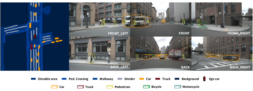
1 Introduction

Taking an image as input, existing vision models usually either ignore (e.g., image classification [28, 10, 6]) or consume directly (e.g., object detection [24, 19, 43], image segmentation [15, 3, 40]) the coordinate frame of input during results prediction. Nonetheless, this paradigm does not match the perception circumstance of self-driving out-of-the-box, where the input source is multiple cameras each with a specific coordinate frame, and the perception models for downstream tasks (e.g., 3D object detection, lane segmentation) need to make predictions in the coordinate frame of the ego car, totally different from all the input frames. That is, a self-driving perception model needs to reason about 3D semantics from 2D visual representations of multi-view images, which is non-trivial and highly challenging.

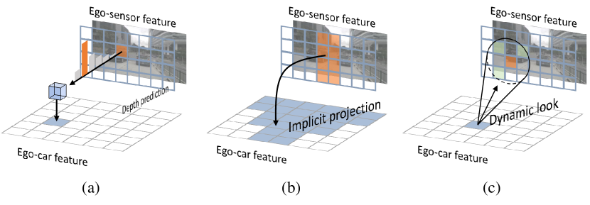
In the literature, existing methods mostly take the following two strategies. The first strategy show in Figure 2(a) (e.g., LSS [22], CaDDN [23]) relies on pixel-level depth estimation, as it can be used to project the 2D visual representation to the ego coordinate frame alongside intrinsic and extrinsic projection. Often, the depth prediction is end-to-end learned within the model without supervision [22], or with extra 3D supervision [23]. A downside of these methods is that depth estimation in unconstrained scenes is typically error-prone, which would be further propagated down to the subsequent components. This is also known as the error propagation problem, largely inevitable for such pipelines.

To solve this above issue, the second strategy (e.g., Image2Map [27], OFT [26], DETR3D [34]) eliminates the depth dimension via directly learning 3D representations from 2D images through architecture innovation. This approach has shown to be superior over depth-estimation based counterparts, implying that learning 3D representation is a superior general strategy. In particular, Image2Map [27] and PON [25] leverage a Transformer or FC layer to learn the projection from 2D image frame to the bird’s-eye-view (BEV) coordinate frame forwardly. As is shown in Figure 2(b), However, their 3D representation is structurally inconsistent with 2D counterparts as no rigorous intrinsic and extrinsic projection can be leveraged, i.e., no explicit one-one correspondence relation across the coordinate frames, consequently resulting in sup-optimal solutions. The recent state-of-the-art DETR3D [34] formulates a 3D representation learning model with a Transformer model, inspired by contemporary image based object detection models [2]. However, its 3D representation is not only sparse, but virtual in the sense of no geometry structure explicitly involved w.r.t the ego coordinate frame, and is thus unable to conduct dense prediction tasks such as segmentation.

In this work, we present a novel ego 3D representation learning method that overcomes all the aforementioned limitations in an end-to-end formulation. This is inspired by the ray tracing principle [35] in computer graphics, which simulates the light transport process from the sources to human eyes in graphic rendering. Rather than taking the optical sources as inception, ray tracing backtracks the optical paths from the imaginary eyes to the objects in an opposite way. Analogously, we start with introducing a polarized grid of dense “imaginary eyes” for BEV representation, with each eye naturally occupying a specific geometry location with the depth information involved. As is shown in Figure 2(c), for learning 3D representation including height information intrinsically absent in BEV, we initialize each eye using a uniform value and leave the eyes to look backward surrounding 2D visual representations subject to the intrinsic and extrinsic 3D-to-2D projection. With the adaptive attention mechanism, eyes focus dynamically on 2D representations and directly learn to approximate missing height information in a data driven manner. Critically, our architecture can be applied for both sparse (e.g., 3D object detection) and dense (e.g., BEV semantic segmentation) prediction tasks. We term our method Ego 3D representation learning as Ray Tracing (Ego3RT).

We make the following contributions: (1) We propose a novel ego 3D representation learning architecture, inspired by the ray tracing perspective. (2) Without depth supervision, our method can learn geometrically structured and dense 3D representations from arbitrary camera rigs w.r.t the ego car coordinate frame, subject to the intrinsic and extrinsic 3D-to-2D projection. This is achieved by adapting the ray tracing concept, where we first introduce a polarized grid of “imaginary eyes” as the learnable BEV representation, and then trace them backwards to camera rigs by formulating the learning process of this 3D representation into an adaptive attention framework. (3) Expensive experiments on 3D object detection and lane segmentation self-driving tasks validate the superiority of our method over state-of-the-art alternative methods, often by a large performance gap. In particular, Ego3RT enables multi-task learning by representation sharing between object detection and BEV segmentation whilst still yielding superior performance, hence more computationally efficient and economically scalable for self-driving.

Figure 2: Comparison of dense 3D representation learning strategies. (a) The first strategy, represented by LSS [22], CaDDN [23], is based on dense pixel-level depth estimation. (b) The second strategy represented by PON [25] bypasses the depth estimation by learning implicit 2D-3D projection. (c) Our strategy that backtracks 2D information from “imaginary” eyes specially designed in the BEV’s geometry.

2 Related work

Depth-based strategy

Benefited from well-studied depth estimation, Pseudo-lidar [33], Pseudo-lidar++ [39] and AM3D [18] separate the 3D representation learning into monocular depth estimation and 3D detection. CaDDN [23] uses a supervised depth estimation network to accumulate a more precise position of each voxel from the front-view features. These dual-step methods rely on extra depth estimation data and are not end-to-end trainable. LSS [22] and FIERY [11] achieve the front-view features lifting in an end-to-end manner with the depth distribution prediction to generate the intermediate 3D representations. However, weakly-constrained depth estimation is error-prone, with the depth error propagated to limit the subsequent 3D localization.

Depth-free strategy

OFT [26] simply hypothesizes a uniform distribution over the depth, leading to poor performance in the 3D detection task. Rather than predicting depth, [37, 4, 25, 27] opt to exploit the 3D-to-2D projection process. PYVA [37] shows that the correspondence between 2D features and 3D features can be implicitly learned by cross attention. NEAT [4] further proposes a variation of cross attention for the same purpose. PON [25] and Image2Map [27] resort to a Transformer or FC layer to learn a correspondence between images and 3D features. While decently estimating the 3D-to-2D relationship, a clear limitation is that these models ignore the intrinsic one-one correspondence. Recently, DETR3D [34] learns sparse 3D representations with a Transformer by using sparse queries to detect 3D objects. However, this 3D representation has no geometry structure, making it incapable of performing dense prediction tasks. In this work, we present Ego3RT, a novel end-to-end trainable ego 3D representation learning architecture that solves all the above limitations. Critically, it can learn 3D ego representation from unconstrained camera rigs without any 3D or depth supervision, achieving superior performance on BEV visual tasks even in a more efficient multi-task model design.

3 Method

Figure 3: Our pipeline comprises two stages: learning ego 3D representation from 2D features and executing multiple downstream tasks based on 3D representation. The gray lines represent the 2D feature stream while the blue lines represent the 3D feature stream. Besides, the orange lines specify our back tracing path.

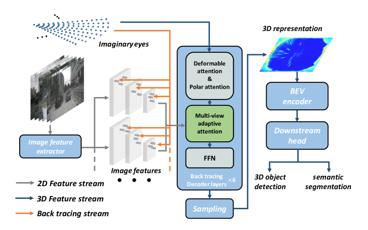
Our architecture can be divided into two components: (1) ego 3D representation learning (Ego3RT) and (2) downstream task head.

3.1 Ego3RT: Ego 3D representation learning

Ego3RT consists of two parts: image feature extractor and back tracing decoder. In addition, to illustrate back tracing decoder clearly, we will first introduce its components – imaginary eyes, tracing 3D backwards to 2D mechanism and multi-view multi-scale adaptive attention.

Image feature extractor

Given a set of images $\mathcal{I}=\{\mathbf{p}_{1},\mathbf{p}_{2},\cdots\mathbf{p}_{N_{\text{view}}}\}$ from multiple camera sensors (i.e., multiple views), where each image $\mathbf{p}_{t}\in\mathbb{R}^{H\times W\times 3}$ with $t$ the index of surrounding cameras (e.g., $N_{\text{view}}=6$ for nuScenes). These images are then encoded by a single shared ego-sensor feature extractor, including a CNN and a transformer encoder. ResNet [10] is used to extract image feature maps at $N_{\text{scale}}$ spatial resolutions. To capture global context information, we further apply a transformer encode [43] at each resolution individually. As a result, we obtain the multi-view multi-scale self-attentive 2D representation $\{\mathbf{x}_{l}^{(t)}\}_{l=1}^{N_{\text{scale}}}$, where $\mathbf{x}_{l}^{(t)}\in\mathbb{R}^{H_{l}\times W_{l}\times C_{l}}$, $H_{l}=\frac{H}{4*2^{l}},W_{l}=\frac{W}{4*2^{l}}$, $t\in[1,\cdots,N_{\text{view}}]$.

Figure 4: An illustration of tracing 3D backwards to 2D mechanism for imaginary eyes. The golden balls represents the polarized grid of dense “imaginary eyes”. Specially, for eyes have multiple visible images (e.g. $\text{eye}_{3}$), they backtrack to multiple images, while eyes having only single visible image (e.g. $\text{eye}_{1}$) backtrack to single image. The blue points on image from light blue to deep show their degree of significance to their eye, thus facilitating the adaptive attention.

Imaginary eyes

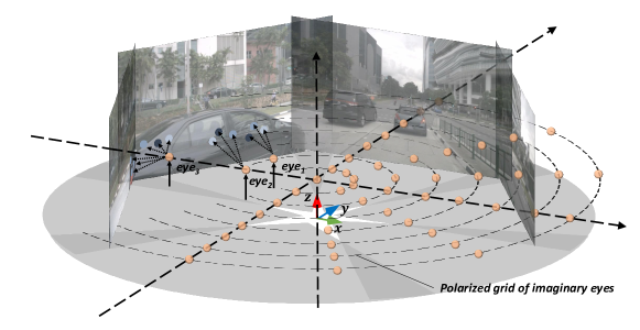
From this part, we will specify how Ego3RT learning 3D representation from 2D. To avoid exhaustive pixel-level prediction and inconsistent coordinate projection, we draw an analogue in the back tracing idea from ray tracing [35]. We start with introducing a polarized grid of dense “imaginary eyes” shown in Figure 4, for BEV representation, with each eye naturally occupying a specific geometry location with built-in depth information. The grid of eyes are in size of $N_{\text{eyes}}=R\times S$, where $R$ is the number of eyes on each polar ray, and $S$ is the number of these polar rays. To construct or, “render” our BEV representation, these imaginary eyes send rays backwards to 2D visual representation following the above 3D-2D projection routine (which will be described later). Since each eye only occupies a single, fixed geometry location, tracing back at its corresponding 2D position alone is less informative due to limited local observation. To solve this problem, we propose to encourage the eyes look around to focus adaptively on pivotal feature points across multiple scale per image and multiple camera views. This results in our multi-view multi-scale adaptive attention module (MVAA). And finally, the features of these imaginary eyes will be the final 3D representation.

Tracing 3D backwards to 2D

To specify the tracing back mechanism, we first illustrate coordinate transformation between 3D and 2D. In typical cases, we usually have one LIDAR coordinate (3D), $N_{\text{view}}$ camera coordinate (3D) and $N_{\text{view}}$ image coordinate (2D). First, a 3D point $\mathbf{x}_{\text{lidar}}=(x,y,z,1)$ in the rectified LIDAR coordinate will be transformed to $\mathbf{x}_{\text{cam}}^{(t)}=(x^{\prime},y^{\prime},z^{\prime},1)$ in the $t^{th}$ rectified camera coordinate with a given matrix $\mathbf{M}_{\text{ex}}^{(t)}$ called extrinsic parameter. Next, $\mathbf{x}_{\text{cam}}^{(t)}=(x^{\prime},y^{\prime},z^{\prime},1)$ is projected to a point $\mathbf{x}_{\text{img}}^{(t)}=(u,v,1)^{\top}$ in the $t^{th}$ image plane by

$$\mathbf{x}_{\text{img}}^{(t)}=\mathbf{M}_{\text{in}}^{(t)}\mathbf{x}_{\text{cam}}^{(t)},\quad\mathbf{M}_{\text{in}}^{(t)}=\left(\begin{array}[]{c c cc cc c}f_{u}^{(t)}&&0&&c_{u}&&-f_{u}^{(t)}b_{x}^{(t)}\\ 0&&f_{v}^{(t)}&&c_{v}&&0\\ 0&&0&&1&&0\end{array}\right)$$ (1)

Here, $\mathbf{M}_{\text{in}}^{(t)}$ is the projection matrix for $t^{th}$ camera. $(f_{u},f_{v})$ is the focal length, $(c_{u},c_{v})$ is the location of optical center and $b_{x}^{(t)}$ denotes the baseline with respect to reference camera ($0$ for nuScenes). In summary, a 3D point $\mathbf{x}_{\text{lidar}}$ can be projected to image point $\mathbf{x}_{\text{img}}^{(t)}$ by the projection matrix $\mathbf{M}^{(t)}=\mathbf{M}_{\text{in}}^{(t)}\mathbf{M}_{\text{ex}}^{(t)}$. In case of $0<u,v<1$, the point will be projected inside the image, otherwise outside. If the $\mathbf{x}_{\text{img}}$ is inside the image, we say that the image is visible to the corresponding $\mathbf{x}_{\text{lidar}}$. In our method, imaginary eyes are encouraged to “look” around their 2D projection point in each image coordinate. We denote the set of visible images of the $q^{th}$ eyes as $\mathcal{I}_{q}\subset\mathcal{I}$.

Multi-view multi-scale adaptive attention (MVAA)

MVAA is the core of transferring 2D representation into 3D. We formulate the learning of these imaginary eyes in an adaptive self-attention detection framework [43]. This is based on an idea of regarding the eyes as object queries, denoted as $\mathbf{y}\in\mathbb{R}^{C\times N_{\text{eye}}}$. Let $\mathbf{r}\in\mathbb{R}^{3\times N_{\text{eye}}}$ be the location of eyes in ego car coordinate. Formally, each eye (i.e., query) will dynamically choose $N_{\text{point}}$ feature points at every scale of 2D image representation. This gives us a total of $N_{\text{scale}}\times|\mathcal{I}_{q}|\times N_{\text{point}}$ feature points. Our MVAA then chooses the most significant feature points from them and fuse them across multiple scales and views into the desired 3D representation. The process can be expressed as

$$\text{MVAA}(\mathbf{y}_{q},\mathbf{r}_{q},\{\{\mathbf{x}_{l}^{(t)}\}_{l=1}^{N_{\text{scale}}}\}_{t=1}^{N_{\text{view}}})=$$

$$\underset{h\in\{N_{h}\}}{\text{concat}}\mathbf{W}_{h}\left[\sum_{l\in\{N_{\text{scale}}\}}\sum_{t\in\mathcal{I}_{q}}\sum_{k\in\{N_{\text{point}}\}}\mathbf{A}_{hltk}\cdot\mathbf{W}^{\prime}_{h}\phi\left(x_{l}^{(t)},\mathbf{\mathbf{M}^{(t)}}\mathbf{r}+\mathbf{\Delta r}_{hvlk}\right)\right]$$ (2)

Vector $\mathbf{y}_{q}$ is the $q^{th}$ query (eye), $\mathbf{r}_{q}$ is its position, $N_{h}$ is the head number, $\mathbf{M}^{(t)}$ is the projection matrix. $\mathbf{A}$ and $\mathbf{\Delta r}$ are conditioned on $\mathbf{y}_{q}$ by learnable parameters:

$$\mathbf{A}=\text{softmax}_{tk}(\mathbf{W}_{q}^{(\mathbf{A})}\mathbf{y}_{q})$$ (3)

with learnable parameter $\mathbf{W}_{q}^{(\mathbf{A})}\in\mathbb{R}^{N_{h}\times N_{\text{scale}}\times|\mathcal{I}_{q}|\times N_{\text{point}}\times C}$, and

$$\mathbf{\Delta r}=\mathbf{W}_{q}^{(\mathbf{r})}\mathbf{y}_{q}+\mathbf{b}_{q}^{(\mathbf{r})}$$ (4)

with learnable parameter $\mathbf{W}_{q}^{(\mathbf{r})}\in\mathbb{R}^{N_{h}\times N_{\text{scale}}\times|\mathcal{I}_{q}|\times N_{\text{point}}\times 2\times C}$, and fixed parameter $\mathbf{b}_{q}^{(\mathbf{r})}\in\mathbb{R}^{N_{h}\times N_{\text{scale}}\times|\mathcal{I}_{q}|\times N_{\text{point}}\times 2}$. To avoid these $N_{\text{point}}$ feature points collapse into one point, $\mathbf{b}_{q}^{(\mathbf{r})}$ is initialized with $|\mathbf{b}_{q}^{(\mathbf{r})}[\cdot,\cdot,\cdot,k]|=k$, so that the more $N_{\text{point}}$, the larger offset of these feature points can be achieved. Therefore, $N_{\text{point}}$ can be utilized to control the receptive field. $\phi(x,r)$ represents access $r^{th}$ feature points from $x$ by index. For adaptively assigning the significance to $N_{\text{scale}}\times|\mathcal{I}_{q}|\times N_{\text{point}}$ points, the Softmax function is applied across all the attended feature points, scales, and views:

$$\sum\limits_{l\in\{N_{\text{scale}}\}}\sum\limits_{t\in\mathcal{I}_{q}}\sum\limits_{k\in\{N_{\text{point}}\}}\mathbf{A}_{hltk}=1$$ (5)

Back tracing decoder

Technically, back tracing decoder takes randomly initialized features of imaginary eyes and scales of 2D feature provided by image feature extractor as input, and finally outputs the fine-grained features of imaginary eyes as 3D representation. Back tracing decoder is made up with a stack of attention layers adapted from the transformer decoder layers [19]. As shown in Figure 3, each layer stacks two self-attention modules and one cross-attention module in order: deformable attention module [43], polar attention and MVAA. Compared to self-attention, deformable attention is more memory efficient. On the on 3D representation, we apply a standard self-attention on the eyes of same polar ray for polar attention. Also, the feed-forward network (FFN) block is equipped with a depth-wise convolution like [32]. As illustrated before, MVAA is responsible for back tracing 2D features into 3D representation.

3.2 Downstream task head design

BEV sampling.

Before the features of imaginary eyes being processed at downstream task, we first grid sample the polarized features into the rectangular ego car coordinate system to match with dataset annotation.

BEV encoder.

To encode the 3D representation for multiple tasks, we adopt the same BEV encoder module from OFT [26]. This kind of sub-network is also widely used in the LiDAR-based 3D detector [36, 13].

Detection head.

A detection head aims to predict the location, dimension, and orientation of an object in 3D space alongside the object category. While the previously mentioned stage has generated a dense BEV features, we adopt the popular 3D detection head from CenterPoint [38] for our detection task without any modification.

Segmentation head.

For the BEV segmentation task, we choose a group of progressive up-sampling convolution-based semantic segmentation decoder heads to deal with different elements from the map. Technically, a $1\times 1$ Conv layer, a batch norm layer with ReLU, and a bilinear upsample Conv layer together form one up-sampling module. The decoder heads for predicting different map elements use the exact BEV features after the BEV encoder.

4 Experiments

4.1 Setup

Dataset.

We evaluate the proposed model on the nuScenes [1] dataset, a large-scale autonomous driving dataset with 1000 driving scenes. Specifically, for multi-camera 3d object detection, it provides streams of images of 6 cameras covering all round from these 1000 scenes, which are then split into 700/150/150 scenes respectively for training, validation, and testing. nuScenes also provide informative annotations of the map. We choose 5 segmentation tasks: drivable area, pedestrian crossing, walkway, carpark, and divider.

Metrics.

To evaluate performance, mean Average Precision (mAP) [8] and NuScenes Detection Score (NDS) [1] are reported. The mAP is the average of precision over different distance thresholds – 0.5m, 1m, 2m, 4m, in bird-eye-view. NDS is averaged weighted by mAP and True Positive (TP) metrics, where TP metrics is mean of five individual metrics: translation (ATE), velocity (AVE), scale (ASE), orientation (AOE), and attribute (AAE) errors. The weighted average is calculated by: $\text{NDS}=\frac{1}{10}\left[5\text{mAP}+\sum_{\text{mTP}\in\mathbb{TP}}(1-\min(1,\text{mTP}))\right]$.

The segmentation task uses Intersection over Union(IoU) to assess the performance. As done by the LSS [22], we create a binary image for each element based on a specific threshold to evaluate with the ground truth image.

Implementation details.

Following FCOS3D [31] and DETR3D [34], ResNet-101 [10], with 3rd and 4th stages equipped with deformable convolutions is applied as our image backbone. The following deformable DETR encoder then utilizes multi-scale feature maps from the 2nd, 3rd, and 4th stages of the backbone. We use eyes of density $80\times 256$ for Ego3RT and be sampled to rectangular $160\times 160$ grids by BEV sampling. For the BEV encoder, we use 8 Bottleneck block [10] identical to OFT [26]. In the segmentation task, we set our ground-truth BEV segmentation map of $480\times 480$ size with 0.2m/pixel resolution. Therefore, 1 block of the upsampling module with the bilinear upsampling ratio of $3\times$ is adopted to mitigate lossing details of the screen. Additionally, Section 0.A.1 illustrates our loss function.

Training & testing.

Our models are trained 24 epoch with AdamW [16] of base learning rate $2.5\times 10^{-4}$ and weightdecay 0.01. Especially, the learning rate of the backbone is 1/10 of the global learning rate and the parameter of batch normalizations of backbone still participate in fine-tuning. To avoid over-fitting, we apply an early stop at 16 epoch. Since a total batch size of 48 across six cameras on eight NVIDIA A6000 GPUs is used, we apply synchronized implementation for every batch normalization. During the training process, we use the input image of $1500\times 900$ resolution with only photometric distortion augmentation. Random flip, random rotation, and random scaling are applied to the 3D feature. Our 3D detection head is trained with class-balanced grouping method [42] (but no DS sampling) as default. After the detection head is well trained, we fix the parameters of Ego3RT and fine-tune our segmentation head for multi-task. Random flip, random rotation, and random scaling are applied to the 3D feature when training detection head while no augmentation are used in multi-task training. Details are explained in Appendix 0.A.2.

4.2 Comparison with state of the art

3D object detection.

Table 1: Comparison of different paradigms on the nuScenes val set. FCOS3D${\dagger}$ is trained with 1x learning schedule, depth weight 0.2 and is finetuned on another FCOS3D checkpoint. PGD${\dagger}$ is trained with 2x learning schedule, depth weight 0.2 on another PGD checkpoint. DETR3D${\dagger}$ and Ego3RT${\dagger}$ are initialized from the same pretrained FCOS3D checkpoint. Ego3RT${\ddagger}$ is initialized from the pretrained DD3D checkpoint.

Methods	mATE$\downarrow$	mASE$\downarrow$	mAOE$\downarrow$	mAVE$\downarrow$	mAAE$\downarrow$	mAP$\uparrow$	NDS$\uparrow$
FCOS3D[31]	0.790	0.261	0.499	1.286	0.167	0.298	0.377
DETR3D[34]	0.860	0.278	0.327	0.967	0.235	0.303	0.374
PGD[30]	0.732	0.263	0.423	1.285	0.172	0.336	0.409
Ego3RT(Ours)	0.714	0.275	0.421	0.988	0.292	0.355	0.409
FCOS3D${\dagger}$[31]	0.754	0.260	0.486	1.331	0.158	0.321	0.395
DETR3D${\dagger}$[34]	0.765	0.267	0.392	0.876	0.211	0.347	0.422
PGD${\dagger}$[30]	0.667	0.264	0.435	1.276	0.177	0.358	0.425
Ego3RT(Ours)${\dagger}$	0.657	0.268	0.391	0.850	0.206	0.375	0.450
Ego3RT(Ours)${\ddagger}$	0.582	0.272	0.316	0.683	0.202	0.478	0.534

We compare our model with previous state-of-the-art methods on both nuScenes validation set and test set. Following FCOS3D [31] and DETR3D [34], all our experiments are trained using ResNet-101 with deformable convolution as backbone for prototype verification. Models without special notification is initialized from a ResNet-101 checkpoint which pre-trained on ImageNet [5]. We also present the result of our model on pre-trained checkpoints from FCOS3D [31] and DD3D [21]. In specific, the DD3D [21] fintunes on extra DDAD15M [9] dataset. To be noted, the monocular-camera paradigms [31, 30] and the multi-camera ones can be fairly compared. They all take 6 cameras as input, but the monocular paradigms process these input images independently while the multi-view paradigms process these input images simultaneously.

Table 1 summarizes our multi-camera 3D object detection results on the nuScenes validation set. The upward arrow means the large the better while the downward one means the small the better. Our method leads in both mAP and NDS. Specially, it achieves the best in transition error (mATE), proving back tracing strategy’s ability in localization reasoning. Just with simple attention, Ego3RT outperforms localization prediction than the well-designed PGD.

Table 2: Comparisons to top-performing works on the nuScenes test set. ${\ddagger}$ represents that the method uses external data other than nuScenes 3D box annotations. DD3D${\ddagger}$ uses extra data for depth estimation. DETR3D${\ddagger}$ and Ego3RT${\ddagger}$ are initialized from the pre-trained DD3D checkpoint.

Methods	mATE$\downarrow$	mASE$\downarrow$	mAOE$\downarrow$	mAVE$\downarrow$	mAAE$\downarrow$	mAP$\uparrow$	NDS$\uparrow$
MonoDIS	0.738	0.263	0.546	1.553	0.134	0.304	0.384
CenterNet [41]	0.658	0.255	0.629	1.629	0.142	0.338	0.400
FCOS3D[31]	0.690	0.249	0.452	1.434	0.124	0.358	0.428
PGD[30]	0.626	0.245	0.451	1.509	0.127	0.386	0.448
Ego3RT(Ours)	0.599	0.268	0.470	1.169	0.172	0.389	0.443
DD3D${\ddagger}$[21]	0.572	0.249	0.368	1.014	0.124	0.418	0.477
DETR3D${\ddagger}$[34]	0.641	0.255	0.394	0.845	0.133	0.412	0.479
Ego3RT(Ours)${\ddagger}$	0.549	0.264	0.433	1.014	0.145	0.425	0.473

Table 3: Comparison of BEV semantic segmentation IoU on the nuScenes val set. Multi means wether generate a full surrounded BEV segmentation map from multi-view images. “-” represents the unprovided result. Single-task version Ego3RT uses EfficientNet-B0 [29] as the image backbone to align with OFT [26] and LSS [22]. Multi-task version Ego3RT$\P$ means we only train the segmentation head with the pretrained detection model frozen.

Method	multi?	Drivable	Crossing	Walkway	Carpark	Divider
VED [17]	✗	54.7	12.0	20.7	13.5	-
VPN [20]	✗	58.0	27.3	29.4	12.3	-
PON [25]	✗	60.4	28.0	31.0	18.4	-
OFT [26]	✗	62.4	30.9	34.5	23.5	-
LSF [7]	✗	61.1	33.5	37.8	25.4	-
Image2Map [27]	✗	74.5	36.6	35.9	31.3	-
OFT [26]	✓	71.7	-	-	-	18.0
LSS [22]	✓	72.9	-	-	-	20.0
Ego3RT(Ours)	✓	79.6	48.3	52.0	50.3	47.5
Ego3RT(Ours) $\P$	✓	74.6	33.0	42.6	44.1	36.6

Table 2 shows our results on the nuScenes test set. The training sets are the same as the validation set. The least transition error (mATE) also reflects the overwhelming localization power of back tracing mechanism. We achieve the best mAP but the NDS is hindered by the attribute error. We have to say that the 2D representation has a manifest advantage on classification over 3D representation.

BEV segmentation.

Table 3 summarizes our BEV segmentation results on nuScenes validation set. We achieve the best performance in all tasks except the pedestrian crossing, but its overwhelming advantage in other tasks still proves its success. We also present single-task version using ImageNet pre-trained Efficient-B0[29] as our image backbone to make a fair comparison with OFT[26] and LSS [22]. In terms of the single-task version, Ego3RT leads the board with huge superiority.

4.3 Qualitative results

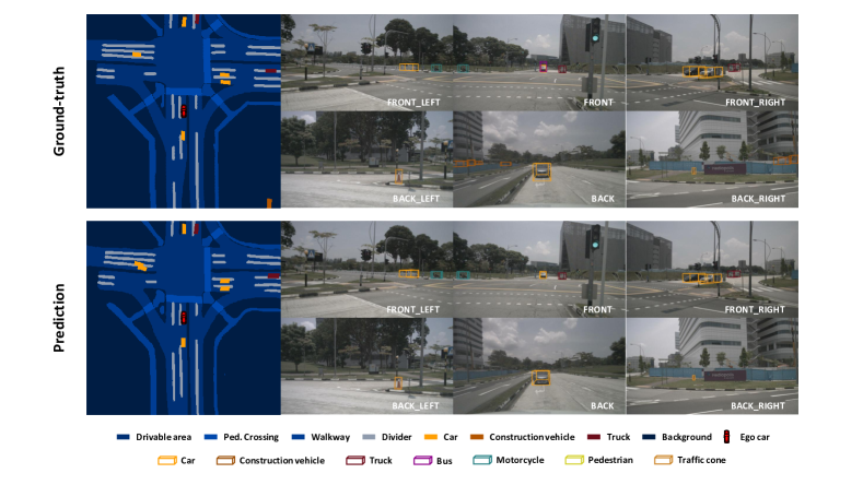
We present our visualization in Figure 5. The structural similarity to the ground-truth highlights the superiority of our Ego3RT, which simultaneously generates dynamic object detection and static semantic segmentation results from the 3D representation. In specific, we project all bounding boxes of class vehicle in nuScenes from the detection head onto the generated BEV segmentation map for a clear comparison. As can be seen from the perspective of images, our detection results demonstrate appealing localization ability even in distance situations. Section 0.A.3 provides more qualitative results

4.4 Ablation studies

In this section, we will figure out how the performance is established and prove the effectiveness of our innovation.

Image backbone.

Table 4: Comparison of different image feature extractors. ${\dagger}$ means the image feature extractor is initialized from a FCOS3D checkpoint. ${\ddagger}$ means the image feature extractor is initialized from a DD3D checkpoint.

Backbone	mATE$\downarrow$	mASE$\downarrow$	mAOE$\downarrow$	mAVE$\downarrow$	mAAE$\downarrow$	mAP$\uparrow$	NDS$\uparrow$
ResNet50	0.706	0.281	0.663	0.964	0.249	0.332	0.380
ResNet101	0.714	0.275	0.421	0.988	0.292	0.355	0.409
ResNet101 ${\dagger}$	0.657	0.268	0.391	0.850	0.206	0.375	0.450
VoveNet${\ddagger}$	0.582	0.272	0.316	0.683	0.202	0.478	0.534

We first provide results with different image feature extractors in Table 4. It presents that the learning of 3D representation relies highly on 2D representation.

Back tracing mechanism

Table 5: Comparisons of detection performance in non-overlap region and overlap region. FCOS3D is trained with 1x learning schedule, depth weight 0.2 and is finetuned on another FCOS3D checkpoint. PGD is trained with 2x learning schedule, depth weight 0.2 and is finetuned on another PGD checkpoint. DETR3D and Ego3RTare initialized from a same pretrained FCOS3D checkpoint.

Methods	overlap?	mATE$\downarrow$	mASE$\downarrow$	mAOE$\downarrow$	mAVE$\downarrow$	mAAE$\downarrow$	mAP$\uparrow$	NDS$\uparrow$
FCOS3D[31]	✗	0.747	0.260	0.487	1.351	0.156	0.320	0.395
PGD[30]	✗	0.658	0.263	0.425	1.290	0.178	0.357	0.426
DETR3D[34]	✗	0.769	0.267	0.390	0.893	0.215	0.343	0.419
Ego3RT(Ours)	✗	0.655	0.267	0.395	0.854	0.208	0.371	0.448
FCOS3D[31]	✓	0.816	0.272	0.571	1.084	0.173	0.229	0.329
PGD[30]	✓	0.768	0.274	0.495	1.090	0.186	0.255	0.354
DETR3D[34]	✓	0.807	0.273	0.453	0.788	0.184	0.268	0.384
Ego3RT(Ours)	✓	0.671	0.268	0.347	0.797	0.212	0.298	0.420

Table 6: Ablation on the effectiveness of adaptive attention mechanism.

adaptive?	mATE$\downarrow$	mASE$\downarrow$	mAOE$\downarrow$	mAVE$\downarrow$	mAAE$\downarrow$	mAP$\uparrow$	NDS$\uparrow$
✗	0.688	0.272	0.403	0.835	0.217	0.365	0.441
✓	0.657	0.268	0.391	0.850	0.206	0.375	0.450

Here, we prove that the back tracing mechanism posses superiority in localization. To eliminate interference of multi-view mechanism, in the top part of Table 5, hence, we validate the 3D detection result only at the non-overlap region where only a monocular camera is used. We show advantage in overall mAP, NDS metrics at monocular region. Specially, the lowest transition error mATE proves the best localization reasoning of Ego3RT .

Multi-view mechanism

We will prove the superiority of the multi-view mechanism over the former monocular ones. In the bottom part of Table 5, we validate the 3D detection result at region where only multiple cameras are used. We find that multi-view methods DETR3D and our Ego3RT outperform mono-view methods FCOS3D [31] and PGD [30] remarkably in all metrics. Additionally, Ego3RT achieves overwhelming performance over the other methods in both mAP and NDS.

Adaptive attention mechanism

We state in the method section that the adaptive attention mechanism can approximate missing height information. All the other conditions remaining the same, we switch off the adaptive attention module by fixing learnable parameter $\mathbf{W}_{q}^{(\mathbf{r})}\mathbf{y}_{q}$ in Eq. (4) to prove its effectiveness. The results shown in Table 6 prove our statement.

Polarized grid of imaginary eyes

Table 7: Ablations on polarized grid of imaginary eyes.

polarized	polar	mATE$\downarrow$	mASE$\downarrow$	mAOE$\downarrow$	mAVE$\downarrow$	mAAE$\downarrow$	mAP$\uparrow$	NDS$\uparrow$
grid?	attention?
✗	✗	0.673	0.271	0.397	0.901	0.211	0.365	0.437
✓	✗	0.656	0.271	0.397	0.881	0.206	0.362	0.440
✓	✓	0.657	0.268	0.391	0.850	0.206	0.375	0.450

We apply a polarized grid of “imaginary eyes” rather than a rectangular grid. Here, we compare these two settings in Table 7. The first line and the second line compare the grid type of eyes without polar attention. Although the polarized grid doesn’t show manifest superiority over the rectangular grid, the polarized grid achieves a remarkable advantage in localization prediction (mATE). Finally, with the help of polar attention on the eyes of each polar ray, the model achieves the best.

Table 8: (a) Results with different density of imaginary eyes. (b) Results with different height above the ground of imaginary eyes in meter.

#eyes	$\mathbf{96\times 256}$	$\mathbf{64\times 256}$	$\mathbf{80\times 224}$	$\mathbf{80\times 256}$
mAP $\uparrow$	0.372	0.366	0.372	0.375
NDS $\uparrow$	0.447	0.444	0.445	0.450

(a)

height	0m	0.4m	0.8m
mAP $\uparrow$	0.375	0.375	0.375
NDS $\uparrow$	0.445	0.437	0.450

(b)

Table 9: Ablation on each component of Ego3RT. For the baseline, we set $N_{point}=1$ (w/o “looking around”), eliminate 3D feature augmentation, adaptive attention mechanism (w/o “adaptive looking”) and polarization (including both polarized grid and polar attention).

Components	mAP$\uparrow$	NDS$\uparrow$
baseline	0.345	0.421
+3D feature augmentation	0.353	0.427
+$N_{point}=3$	0.360	0.433
+adaptive attention	0.365	0.437
+polarization	0.375	0.450

Density of imaginary eyes

In this section, we compare imaginary eyes of different densities. Lower density will lead to coarser feature maps while the higher density imposes a burden on optimization, so a balance should be achieved. Table 8b(a) shows that our final choice $80\times 256$ is the optimal choice.

Height of imaginary eyes

Since we use the imaginary eyes occupied at a pre-given location, the height is a hyper-parameter. We compares different choice of height in Table 8b(b). It shows that no significant difference exists among the different choices of height.

Which leads to improvement

To further clarify, we summarize the effect of each component in Table 9, including 3D feature augmentation, the choice of $N_{point}$, adaptive attention mechanism, polarized grid and polar attention. Importantly, each component of our Ego3RT yields good gain.

Table 10: Comparison of the efficiency and the performance of different configurations of Ego3RT and the other methods. “FPS” is a metric for efficiency standing for frames per second. “Resolution” represents input image shape. “FFN” represents the channel expansion dimension of FFN in Back tracing decoder. “Blocks” notes the number of blocks in BEV encoder. “$\star$” means we test the speed at $1600\times 900$.

Methods	Resolution	Eyes density	FFN	#Blocks	FPS$\uparrow$	mAP$\uparrow$	NDS$\uparrow$
FCOS3D[31]	$1600\times 900$	-	-	-	2.0	0.321	0.395
PGD [30]	$1600\times 900$	-	-	-	1.5	0.358	0.425
DETR3D [34]	$1600\times 900$	-	-	-	3.0	0.347	0.422
Ego3RT(Ours)	$1600\times 900^{\star}$	$80\times 256$	1024	8	1.7	0.375	0.450
Ego3RT(Ours)	$1280\times 768$	$72\times 192$	1024	8	2.3	0.372	0.438
Ego3RT(Ours)	$1280\times 768$	$64\times 128$	256	2	3.0	0.355	0.423

Efficiency of Ego3RT

We compare the efficiency and performance of different Ego3RT configurations and the other methods in Table 10. Our Ego3RT (of main configuration) achieves the best mAP and 3rd FPS, and Ego3RT with smaller input image size and imaginary eyes density barely looses its performance while achieves a better efficiency. When Ego3RT further reduces its eyes density, FFN channel expansion dimension and BEV encoder blocks, it reaches the best trade-off between accuracy and efficiency.

Figure 5: Qualitative results on nuScenes dataset. Left is the BEV segmentation map with projected vehicle 3D bounding boxes result from detection head. Right are in image perspective with prediction results. Different colors stand for different categories.

5 Conclusion

In this work, we have presented Ego3RT, a novel end-to-end architecture for ego 3D representation learning given multiple unconstrained camera views. In the absence of depth or 3D supervision, it can learn rich and semantic 3D representation with multi-view images efficiently in the ego car coordinate frame. This is realized by drawing an analog from the ray tracing concept, where we create a polarized grid of learnable “imaginary eyes” as the ego 3D representation and formulate the learning with the adaptive attention mechanism subject to the 3D-to-2D projection. It is easy to implement and able to support multiple different tasks. Extensive experiments validate the superiority of our Ego3RT in comparison to state-of-the-art alternatives in terms of both accuracy and versatility.

Appendix 0.A Appendix

0.A.1 Objective functions

There are two training objectives for our model, including the loss $\mathcal{L}_{det}$ for object detection, and the loss $\mathcal{L}_{seg}$ for map elements segmentation:

$$\mathcal{L}=\mathcal{L}_{cls}+\mathcal{L}_{seg}.$$ (6)

Detection

To handle the severe class imbalance with the nuScenes dataset, following CBGS [42] we group the similar classes into the same sub-task head. We use the focal loss for classification to alleviate the sample imbalance during our training, and simply adopt $L1$ loss to regress the normalized box parameters.

The classification loss for a specific sub-task $\mathcal{L}_{cls}^{t}$ is formulated as follows:

$$\begin{array}[]{r}\mathcal{L}_{cls}^{t}=-\frac{1}{N}\sum_{y_{cls}\in Y_{cls}}\begin{cases}(1-\hat{y}_{cls})^{\alpha}\log(\hat{y}_{cls})&\!\text{if}\ y_{cls}=1\vspace{2mm}\\ \begin{array}[]{c}(1-y_{cls})^{\beta}(\hat{y}_{cls})^{\alpha}\log(1-\hat{y}_{cls})\end{array}&\!\text{otherwise}\end{cases},\end{array}$$ (7)

where $Y_{cls}$ and N represents the set of pixels on the heatmap and the number of objects in $t$-th group, respectively. $\hat{y}_{cls}$ is the predicted classification probability and ${y}_{cls}$ is the ground-truth. $\alpha$ and $\gamma$ are the parameters of the focal loss[14].

The 3D bounding box regression loss for a specific sub-task $\mathcal{L}_{box}^{t}$ could be formulated as:

$$\mathcal{L}_{box}^{t}=\sum_{res\in\mathcal{R}}\mathcal{L}_{L1}(\widehat{\Delta_{res}},\Delta_{res}),$$ (8)

where $\widehat{\Delta_{res}}$ is the predicted residual for the candidate center and $\Delta_{res}$ is the target ground-truth. $\mathcal{R}$ is the set of a box parameters, where $x,y$ are the refinement for the location, $z$ stands for the height, $l,h,w$ are the 3D bounding box size, $\sin{\theta}$ and $\cos{\theta}$ are the rotation at yaw angel, $v_{x}$, $v_{y}$ represent the velocities of the object.

Therefore, the overall detection loss $\mathcal{L}_{det}$ is formulated:

$$\mathcal{L}_{det}=\sum_{t\in\mathcal{T}_{det}}(\lambda_{cls}\mathcal{L}_{cls}^{t}+\lambda_{box}\mathcal{L}_{box}^{t}),$$ (9)

where $\mathcal{T}_{det}$ stands for the set of sub-task groups, $\lambda_{cls}$ and $\lambda_{box}$ represent the loss weights for classification and box regression.

Segmentation

We use 5 different segmentation heads for the static elements in the BEV map, and the pixel-wise binary cross-entropy loss $\mathcal{L}_{seg}^{t}$ for $t$-th sub-task. The overall segmentation loss $\mathcal{L}_{seg}$ is computed as follows:

$$\mathcal{L}_{seg}=\sum_{t\in\mathcal{T}_{seg}}\lambda_{seg}^{t}\mathcal{L}_{seg}^{t},$$ (10)

where $\mathcal{T}_{seg}$ represents the set of elements in the BEV map, $\lambda_{seg}^{t}$ is the loss weight of the element.

0.A.2 Additional training & testing details

When training detection head, rotation degree is uniformly selected from $-22.5^{\circ}\sim 22.5^{\circ}$ to perform random rotation. Then, scale ration is uniformly selected from $0.95\sim 1.05$ to perform random scale. Next, horizontal flip and vertical flip are uniformly selected to perform random flip. All the augmentations are applied in 50% probability. Critically, to make fair comparison, no 3D feature augmentation are used in BEV segmentation training and no test time augmentation in all tasks. The effectiveness of 3D feature augmentation is shown in Table 9 that the augmentation brings 2% improvement to mAP. However, [12] states that the 3D feature augmentation brings at least 20% improvement to a depth-based method. It reveals that the 3D representation generated by the depth-based method [22] (3D-2D relationship is based on depth estimation with only a few convolution layers) suffers severe over-fitting in detection tasks without 3D augmentation. In contrast, 3D-2D relationship of our Ego3RT shows a robustness with the help of adaptive attention mechanism.

0.A.3 Additional qualitative results

Visualization with video

On our page, we simultaneously generate visualization of dynamic object detection and static semantic segmentation results from the 3D representation. In specific, we project all bounding boxes of class vehicle in nuScenes from the detection head onto the generated BEV segmentation map for a clear comparison.

Visualization of object detection results

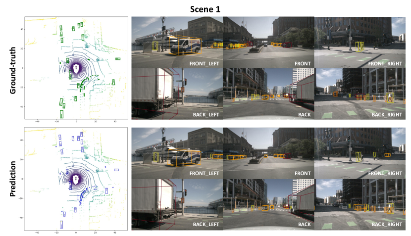
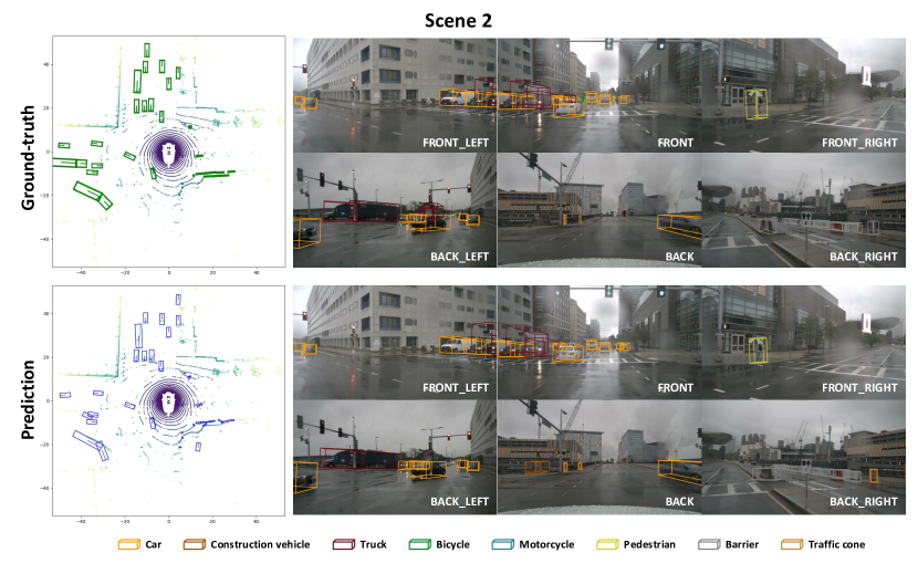
Figure 8 presents visualization of object detection results of two scenes in nuScenes val set. We have the following observations. (i) Ego3RT yields precise localization regarding to the bird’s-eye-view visualization, even for the objects at long distance. (ii) Ego3RT can still work well in rainy whether shown in the second scene, proving its robustness to the whether condition. (iii) There are some miss-labeling in this dataset. For example, traffic cone in the BACK_RIGHT image of second scene is mis-labeled as barrier, but Ego3RT correctly labels it as traffic cone.

Visualization of 3D representation

Figure 6: Visualization results of 2 scenes’ 3D representations given by Ego3RT. For each scene, left is the ground-truth of objects in bird’s-eye view, while right is the visualization of 3D representation. Colors closer to Red represent higher response while colors closer to Blue represent lower response.

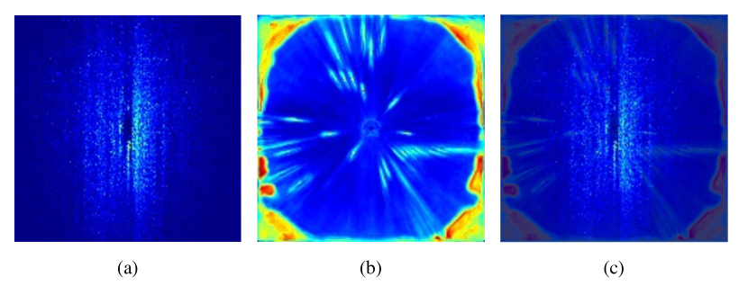
We provide the visualization of Ego3RT’s learned 3D representation of the same scenes shown in the last section in Figure 6. The 3D representations predicted by Ego3RT are simply taken average on the channel to visualize. There is clear activation in the 3D representation wherever there is an object. The visualization demonstrates that Ego3RT actually learns 3D dense representation.

Objects’ localization distribution

There is an interesting observation that the outer part of 3D representation has different pattern in comparison with the inner part. At the beginning, we considered it was caused by the error in codes, but this different pattern remained even after a careful inspection. It is not until we visualized the objects’ localization distribution of nuScenes that the answer was uncovered. Objects in nuScenes dataset appear more frequently at the center than the surrounding area. As is shown in Figure 7(c), the boundary of 3D representation’s inner part well matches that of the objects’ localization distribution. Therefore, Ego3RT reveals some data distribution while reasoning the 3D representation.

Figure 7: (a) Distribution (heat map) of object localization in bird’s-eye-view on nuScenes dataset. Colors closer to Red represent higher frequency while colors closer to Blue represent lower frequency. (b) 3D representation generated by Ego3RT. Colors closer to Red represent higher response while colors closer to Blue represent lower response. (c) Distribution of object localization with the 3D representation, in the same coordinate as bird’s-eye-view.

(a)

(b)

Figure 8: Qualitative results on nuScenes dataset. Two scenes with both ground-truth and prediction are shown. Left are bird’s-eye-view visualizations of object detection results. Right are in image perspective with prediction results. Different colors stand for different categories.

References

- [1] Caesar, H., Bankiti, V., Lang, A.H., Vora, S., Liong, V.E., Xu, Q., Krishnan, A., Pan, Y., Baldan, G., Beijbom, O.: nuscenes: A multimodal dataset for autonomous driving. In: CVPR (2020)
- [2] Carion, N., Massa, F., Synnaeve, G., Usunier, N., Kirillov, A., Zagoruyko, S.: End-to-end object detection with transformers. In: ECCV (2020)
- [3] Chen, L.C., Papandreou, G., Schroff, F., Adam, H.: Rethinking atrous convolution for semantic image segmentation. arXiv preprint (2017)
- [4] Chitta, K., Prakash, A., Geiger, A.: Neat: Neural attention fields for end-to-end autonomous driving. In: ICCV (2021)
- [5] Deng, J., Dong, W., Socher, R., Li, L.J., Li, K., Fei-Fei, L.: Imagenet: A large-scale hierarchical image database. In: CVPR (2009)
- [6] Dosovitskiy, A., Beyer, L., Kolesnikov, A., Weissenborn, D., Zhai, X., Unterthiner, T., Dehghani, M., Minderer, M., Heigold, G., Gelly, S., et al.: An image is worth 16x16 words: Transformers for image recognition at scale. In: ICLR (2021)
- [7] Dwivedi, I., Malla, S., Chen, Y.T., Dariush, B.: Bird’s eye view segmentation using lifted 2d semantic features. In: BMVC (2021)
- [8] Everingham, M., Van Gool, L., Williams, C.K., Winn, J., Zisserman, A.: The pascal visual object classes (voc) challenge. IJCV (2010)
- [9] Guizilini, V., Ambrus, R., Pillai, S., Raventos, A., Gaidon, A.: 3d packing for self-supervised monocular depth estimation. In: CVPR (2020)
- [10] He, K., Zhang, X., Ren, S., Sun, J.: Deep residual learning for image recognition. In: CVPR (2016)
- [11] Hu, A., Murez, Z., Mohan, N., Dudas, S., Hawke, J., Badrinarayanan, V., Cipolla, R., Kendall, A.: Fiery: Future instance prediction in bird’s-eye view from surround monocular cameras. In: CVPR (2021)
- [12] Huang, J., Huang, G., Zhu, Z., Du, D.: Bevdet: High-performance multi-camera 3d object detection in bird-eye-view. arXiv preprint (2021)
- [13] Lang, A.H., Vora, S., Caesar, H., Zhou, L., Yang, J., Beijbom, O.: Pointpillars: Fast encoders for object detection from point clouds. In: CVPR (2019)
- [14] Lin, T.Y., Goyal, P., Girshick, R., He, K., Dollár, P.: Focal loss for dense object detection. In: ICCV (2017)
- [15] Long, J., Shelhamer, E., Darrell, T.: Fully convolutional networks for semantic segmentation. In: CVPR (2015)
- [16] Loshchilov, I., Hutter, F.: Decoupled weight decay regularization. In: ICLR (2019)
- [17] Lu, C., van de Molengraft, M.J.G., Dubbelman, G.: Monocular Semantic Occupancy Grid Mapping With Convolutional Variational Encoder-Decoder Networks. IEEE Robotics and Automation Letters (2019)
- [18] Ma, X., Wang, Z., Li, H., Zhang, P., Ouyang, W., Fan, X.: Accurate monocular 3d object detection via color-embedded 3d reconstruction for autonomous driving. In: ICCV (2019)
- [19] Misra, I., Girdhar, R., Joulin, A.: An end-to-end transformer model for 3d object detection. In: ICCV (2021)
- [20] Pan, B., Sun, J., Leung, H.Y.T., Andonian, A., Zhou, B.: Cross-view semantic segmentation for sensing surroundings. IEEE Robotics and Automation Letters (2020)
- [21] Park, D., Ambrus, R., Guizilini, V., Li, J., Gaidon, A.: Is pseudo-lidar needed for monocular 3d object detection? In: ICCV (2021)
- [22] Philion, J., Fidler, S.: Lift, splat, shoot: Encoding images from arbitrary camera rigs by implicitly unprojecting to 3d. In: ECCV (2020)
- [23] Reading, C., Harakeh, A., Chae, J., Waslander, S.L.: Categorical depth distribution network for monocular 3d object detection. In: CVPR (2021)
- [24] Ren, S., He, K., Girshick, R., Sun, J.: Faster r-cnn: Towards real-time object detection with region proposal networks. In: NeurIPS (2015)
- [25] Roddick, T., Cipolla, R.: Predicting semantic map representations from images using pyramid occupancy networks. In: CVPR (2020)
- [26] Roddick, T., Kendall, A., Cipolla, R.: Orthographic feature transform for monocular 3d object detection. In: BMVC (2019)
- [27] Saha, A., Maldonado, O.M., Russell, C., Bowden, R.: Translating images into maps. arXiv preprint (2021)
- [28] Simonyan, K., Zisserman, A.: Very deep convolutional networks for large-scale image recognition. ICLR (2015)
- [29] Tan, M., Le, Q.: Efficientnet: Rethinking model scaling for convolutional neural networks. In: ICML (2019)
- [30] Wang, T., Xinge, Z., Pang, J., Lin, D.: Probabilistic and geometric depth: Detecting objects in perspective. In: Conference on Robot Learning (2022)
- [31] Wang, T., Zhu, X., Pang, J., Lin, D.: Fcos3d: Fully convolutional one-stage monocular 3d object detection. In: CVPR (2021)
- [32] Wang, W., Xie, E., Li, X., Fan, D.P., Song, K., Liang, D., Lu, T., Luo, P., Shao, L.: Pvt v2: Improved baselines with pyramid vision transformer. Computational Visual Media pp. 415–424 (2022)
- [33] Wang, Y., Chao, W.L., Garg, D., Hariharan, B., Campbell, M., Weinberger, K.Q.: Pseudo-lidar from visual depth estimation: Bridging the gap in 3d object detection for autonomous driving. In: CVPR (2019)
- [34] Wang, Y., Guizilini, V.C., Zhang, T., Wang, Y., Zhao, H., Solomon, J.: Detr3d: 3d object detection from multi-view images via 3d-to-2d queries. In: Conference on Robot Learning (2022)
- [35] Whitted, T.: An improved illumination model for shaded display. In: ACM Siggraph 2005 Courses (2005)
- [36] Yan, Y., Mao, Y., Li, B.: Second: Sparsely embedded convolutional detection. Sensors (2018)
- [37] Yang, W., Li, Q., Liu, W., Yu, Y., Ma, Y., He, S., Pan, J.: Projecting your view attentively: Monocular road scene layout estimation via cross-view transformation. In: CVPR (2021)
- [38] Yin, T., Zhou, X., Krahenbuhl, P.: Center-based 3d object detection and tracking. In: CVPR (2021)
- [39] You, Y., Wang, Y., Chao, W.L., Garg, D., Pleiss, G., Hariharan, B., Campbell, M., Weinberger, K.Q.: Pseudo-lidar++: Accurate depth for 3d object detection in autonomous driving. In: ICLR (2019)
- [40] Zheng, S., Lu, J., Zhao, H., Zhu, X., Luo, Z., Wang, Y., Fu, Y., Feng, J., Xiang, T., Torr, P.H., et al.: Rethinking semantic segmentation from a sequence-to-sequence perspective with transformers. In: CVPR (2021)
- [41] Zhou, X., Wang, D., Krähenbühl, P.: Objects as points. arXiv preprint (2019)
- [42] Zhu, B., Jiang, Z., Zhou, X., Li, Z., Yu, G.: Class-balanced grouping and sampling for point cloud 3d object detection. arXiv preprint (2019)
- [43] Zhu, X., Su, W., Lu, L., Li, B., Wang, X., Dai, J.: Deformable detr: Deformable transformers for end-to-end object detection. In: ICLR (2021)