Efficient inference for Kendall’s tau

Abstract

Kendall’s tau is a nonparametric measure of correlation. We present an efficient method for computing the empirical estimate of Kendall’s tau and the jackknife estimate of its variance. For datasets of fixed dimension, the algorithm’s runtime is log-linear in the number of observations. This is achieved by modifying the standard algorithm for computing the empirical Kendall’s tau to return estimates of the summands making up its Hájek projection.

1 Introduction

Kendall’s $\tau$ is a nonparametric measure of association between two random variables (population version, $\tau$) or between two sets of observations (sample version, $\hat{\tau}$) which is particularly useful for copula models, as many of these can be parametrized in terms of $\tau$ (Nelsen, , 2006, Section 5.1.1; McNeil et al., , 2015, Proposition 7.32 and Section 7.5.1). It appears in statistical procedures spanning fields such as survival analysis (Martin and Betensky, , 2005; Lakhal et al., , 2008), hydrology (Hamed, , 2011; Lebrenz and Bárdossy, , 2017) and risk management (McNeil et al., , 2015), to name a few, as well as in several recently proposed tests of independence (Bergsma and Dassios, , 2014; Mao, , 2018; Leung and Drton, , 2018). In this paper, we present an algorithm for efficiently computing the jackknife estimate of the variance of $\hat{\tau}$, which plays a central role in the works of Chen, (2018) and Perreault et al., 2022a . With its log-linear runtime in the number of observations, it allows fast inference based on $\hat{\tau}$ and can dramatically speedup simulations that require its computation. This compares favourably with the $O(n^{2})$ computational complexity of the methods used by Perreault et al., 2022a and by Martin and Betensky, (2005) for computing the jackknife estimate of the variance of the standard and so-called conditional Kendall’s $\hat{\tau}$, respectively.

Consider a dataset $\{(X_{i},Y_{i})\}_{i=1}^{n}$ of $n$ independent replicates of a continuous random vector $(X,Y)$, so that $X_{i}\neq X_{j}$ and $Y_{i}\neq Y_{j}$ with probability one for all $i\neq j$. We exploit the convenient characterization of $\hat{\tau}$, seemingly due to Esscher, (1924), as a function of the concordance: For $i\neq j$, $(X_{i},Y_{i})$ and $(X_{j},Y_{j})$ are concordant if $(X_{i}-X_{j})(Y_{i}-Y_{j})>0$ and discordant otherwise. Then, $\hat{\tau}$ can be defined as

$$\hat{\tau}:=\frac{c-d}{c+d}=1-\frac{2d}{\binom{n}{2}}=\frac{2c}{\binom{n}{2}}-1,$$ (1)

where $c:=\sum_{i<j}\mathbbm{1}\{(X_{i}-X_{j})(Y_{i}-Y_{j})>0\}$ and $d:=\sum_{i<j}\mathbbm{1}\{(X_{i}-X_{j})(Y_{i}-Y_{j})<0\}$ denote the numbers of concordant and discordant pairs of observations, respectively, and $c+d=\binom{n}{2}$. Similarly, $\tau:=\mathbb{P}\{(X_{1}-X_{2})(Y_{1}-Y_{2})>0\}-\mathbb{P}\{(X_{1}-X_{2})(Y_{1}-Y_{2})<0\}$.

Following Hoeffding, (1948), $\hat{\tau}$ is a non-degenerate $U$-statistic of order two with kernel $h:(X_{1},Y_{1};X_{2},Y_{2})\mapsto 2\mathbbm{1}\{(X_{1}-X_{2})(Y_{1}-Y_{2})>0\}-1$. It is thus an unbiased and asymptotically normal estimator of $\tau$ as $n\to\infty$, i.e., $\sqrt{n}(\hat{\tau}-\tau)\rightsquigarrow\mathcal{N}(0,\sigma^{2})$ for some $\sigma>0$. The standard proof of this uses the Hájek projection $H$ of $\hat{\tau}-\tau$, i.e.,

$$H:=\sum_{i=1}^{n}\mathbb{E}(\hat{\tau}-\tau|X_{i},Y_{i})=\frac{2}{n}\sum_{i=1}^{n}g(X_{i},Y_{i}),$$ (2)

where $g(x,y):=\mathbb{E}\{h(x,y;X,Y)\}-\tau$ (Hájek, , 1968). More explicitely, $g(x,y)=2\{F(x,y)+\bar{F}(x,y)\}-1-\tau$, where $F$ and $\bar{F}$ denote the joint distribution function and survival function of $(X,Y)$, respectively. As is well known, $\sqrt{n}(\hat{\tau}-\tau-H)\to 0$ in probability as $n\to\infty$, so that asymptotic normality follows from the central limit theorem, and $\sigma^{2}=4\mathbb{V}\mathrm{ar}\{g(X,Y)\}$ (van der Vaart, , 1998, Section 12). See, e.g., Genest et al., (2011) for a more detailed presentation of the asymptotic properties of $\hat{\tau}$ in the classical framework.

The aforementioned result generalises to higher dimensions as well. Say the random vector under study is of dimension $p$ and let $p_{2}=\binom{p}{2}$ be the total number of pairs of variables. Also let $\bm{\hat{\tau}}$, $\bm{\tau}$ and $\bm{g}$ be the natural $p_{2}$-dimensional extensions of $\hat{\tau}$, $\tau$ and $g$, respectively. Then, we have that $\sqrt{n}(\bm{\hat{\tau}}-\bm{\tau})\rightsquigarrow\mathcal{N}(\bm{0},\bm{\Sigma})$ as $n\to\infty$ with $\bm{\Sigma}=4\mathbb{V}\mathrm{ar}\{\bm{g}\}$. This holds whenever $p$ is fixed and, up until recently, not much was known about the behaviour of $\sqrt{n}(\bm{\hat{\tau}}-\bm{\tau})$ when $p$ is allowed to grow with $n$. For this latter situation, a notable advance was made by Chen, (2018), who establishes a nonasymptotic error bound for the supremum distance, over hyperrectangles, between the distribution of $\sqrt{n}(\bm{\hat{\tau}}-\bm{\tau})$ and that of the $p_{2}$-dimensional random vector $\bm{Z}\sim\mathcal{N}(\bm{0},\bm{\Sigma})$, i.e., for

$$\sup\nolimits_{A\in\mathcal{A}}|\mathbb{P}\{\sqrt{n}(\bm{\hat{\tau}}-\bm{\tau})\in A\}-\mathbb{P}\{\bm{Z}\in A\}|,$$

where $\mathcal{A}$ is the set of all hyperrectangles in $\mathbb{R}^{p_{2}}$. The bound, which is asymptotically valid when $p_{2}$ is as large as $O(\exp n^{\gamma})$ for some constant $\gamma\in(0,1/7)$, actually applies (under certain conditions) to arbitrary nondegenerate, centered U-statistics.

In order to perform inference based on $\bm{\hat{\tau}}$, one is required to estimate $\bm{\Sigma}$, either explicitly or implicitly. To this end, the rescaled jackknife (hereinafter simply jackknife) estimator of $\bm{\Sigma}$, which we denote by $\bm{\hat{\Sigma}}$, has attracted considerable attention recently. In particular, it was shown that $\bm{\hat{\Sigma}}$ was suitable for inference in both classical (Rublík, , 2016; Perreault et al., 2022a, ) and high-dimensional (Chen, , 2018; Perreault et al., 2022a, ) settings. When $p=2$, so that $\bm{\Sigma}=\sigma^{2}$ reduces to a single entry, it is given by

$$\hat{\sigma}^{2}:=\frac{4}{n}\sum_{i=1}^{n}\hat{g}_{i}^{2},\qquad\text{with }\hat{g}_{i}:=\frac{1}{n-1}\sum_{j\neq i}h(X_{i},Y_{i};X_{j},Y_{j})-\hat{\tau},$$ (3)

where $\hat{g}_{i}$ can be interpreted as an empirical estimator of $g(X_{i},Y_{i})$. Note that we focus here on the bivariate case only to avoid cumbersome notation; the jackknife estimator of $\bm{\Sigma}$ is simply $\bm{\hat{\Sigma}}=(4/n)\sum_{i=1}^{n}\bm{\hat{g}}_{i}\bm{\hat{g}}_{i}^{\top}$ for some vectors $\bm{\hat{g}}_{i}$ whose components are of same form as $\hat{g}_{i}$ in (3). Given $\hat{g}_{1},\dots,\hat{g}_{n}$, computing $\hat{\sigma}^{2}$ amounts to a standard variance calculation that can be done in linear time in $n$. Thus, when using (3) to explicitely compute $\hat{\sigma}^{2}$, the main computational challenge is to compute the estimates $\hat{g}_{1},\dots,\hat{g}_{n}$.

Our main contribution is to provide an efficient method for computing $\hat{g}_{1},\dots,\hat{g}_{n}$. This is achieved by modifying the well-known $O(n\log_{2}n)$ algorithm of Knight, (1966) for computing $\hat{\tau}$, or more precisely its implementation in the R package pcaPP (Filzmoser et al., , 2018). In Section 2, we review the idea underlying Knight’s algorithm. In Section 3, we present the main result upon which our algorithm is based. In Section 4, we explain how to implement the algorithm and we compare its runtime with popular functions used to compute $\hat{\tau}$. In Section 5, we illustrate the effectiveness of our method in an application for which $p=50$. Section 6 concludes the paper.

The proposed algorithm is detailed in pseudocode in Appendix A. An implementation in R, used to carry out the analyses of Sections 4 and 5, is provided as online supplementary material.

2 Standard algorithm for computing $\bm{\hat{\tau}}$

2.1 General idea

The computation of $\hat{\tau}$ is intimately related to the $O(n^{2})$ sorting algorithm called exchange sort or sorting by exchanging (Kendall, , 1948): A list of numbers to be sorted is scanned and every time two adjacent numbers not in order are encountered, the pair is exchanged. Scanning is repeated until the list is in order (Knight, , 1966). When the vector of observations $\bm{X}:=(X_{1},\dots,X_{n})$ is already sorted in increasing order ($X_{1}<\dots<X_{n}$), the number of discordant observations $d$ appearing in (1) coincides with the number of swaps required to sort $\bm{Y}:=(Y_{1},\dots,Y_{n})$ using exchange sort. In other words, to compute $\hat{\tau}$ one can first jointly reorder $\bm{X}$ and $\bm{Y}$ (using any sorting algorithm) so that $\bm{X}$ is in increasing order and then sort the resulting $\bm{Y}$, this time keeping track of the number of swaps required.

The main contribution of Knight, (1966) was to exploit the ability of merge sort algorithms to sort a list in $O(n\log_{2}n)$ operations while keeping track of the number of swaps that naive exchange sort would have required. Assuming for simplicity that the list of elements to be sorted, $\bm{Y}$ in our case, is of length $n=2^{K}$ for some $K\in\mathbb{N}$, Knight’s merge sort algorithm first partitions $\bm{Y}$ into $2^{K-0}$ sublists of length $2^{0}=1$ and then recursively (a) merges the sublists in pairs and (b) sorts within each newly created sublist. After a first application of the recursive steps, the algorithm produces $2^{K-1}$ sorted sublists of size $2^{1}$; after a second application, it produces $2^{K-2}$ sorted sublists of size $2^{2}$; and so on until the entire list of length $2^{K}$ is sorted.

The efficiency of this strategy comes from the fact that each sublist of size $2^{k}$ is the concatenation of two sorted sublists of size $2^{k-1}$, making it easier to sort than an arbitrary unsorted sublist of the same size. To see why, let $\bm{a}=(a_{1},\dots,a_{m})$ and $\bm{b}=(b_{1},\dots,b_{m})$ be sorted lists and consider sorting their concatenation $(\bm{a},\bm{b})$. In the extreme event that $a_{m}<b_{1}$, a single comparison suffices to conclude that $a_{i}<b_{j}$ for all $i,j\in\{1,\dots,m\}$ and that no swap is required. Similarly, if $a_{1}>b_{m}$, then a single comparison suffices to conclude that $a_{i}>b_{j}$ for all $i,j\in\{1,\dots,m\}$, that $m^{2}$ swaps are required, and that $(\bm{b},\bm{a})$ is sorted.

We refer the reader to Knuth, (1998) or Cormen et al., (2014) for a detailed presentation of sorting algorithms. See also Abrevaya, (1999) and Christensen, (2005) for related discussions about computing $\hat{\tau}$.

2.2 Mathematical formulation

We now provide a slightly more formal description of sorting by exchanging. For the rest of the paper, we assume that $\bm{X}$ is already ordered ($X_{1}<\dots<X_{n}$). We use $\bm{Y}^{*}$ to denote the ordered version of $\bm{Y}$, that is, $\bm{Y}^{*}:=(Y_{(1)},\dots,Y_{(n)})$ where for each $i\in\{1,\dots,n\}$, $Y_{(i)}$ is the $i$th order statistic of $\bm{Y}$ ($Y_{(1)}<\dots<Y_{(n)}$), and we denote by $\pi$ the permutation of $n$ elements that yields $\pi(\bm{Y})=\bm{Y}^{*}$.

By definition, any application of exchange sort can be expressed as a composition $\pi_{j_{m}}\circ\dots\circ\pi_{j_{1}}$ ($m\in\mathbb{N}$) of permutations $\pi_{j}$ ($j\in\{1,\dots,n-1\}$) of the form

$$\{\pi_{j}(\bm{y})\}_{i}:=\begin{cases}y_{i-1}&\quad\text{if }i=j+1\\ y_{i+1}&\quad\text{if }i=j\\ y_{i}&\quad\text{otherwise,}\end{cases}$$

where $\bm{y}\in\mathbb{R}^{n}$. In other words, $\pi_{j}$ simply swaps the $j$th and $(j+1)$th components of the vector to which it is applied. The representation $\pi=\pi_{j_{m}}\circ\dots\circ\pi_{j_{1}}$ of $\pi$ is not unique in general, since at any given step of the algorithm, there might be several pairs of adjacent observations that need to be swapped. However, it turns out that any representation ensuing from sorting by exchanging is minimal, in the sense that $m$ is as small as possible.

To obtain a minimal representation, one must ensure that two components of the original vector $\bm{Y}$ are swapped together at most once. Sorting by exchanging is specifically designed to satisfy this requirement, as two adjacent elements are swapped only if necessary, i.e., if they are in the wrong order ($Y_{i}>Y_{j}$ with $i<j$); once two elements are swapped, they can never be swapped again. Because each permutation $\pi_{j_{k}}$ ($k=1,\dots,m$) removes exactly one discordance, exactly $m=d$ of them are required to reorder $\bm{Y}$. Mathematically, recalling that $\mathbbm{1}(X_{i}<X_{j},Y_{i}<Y_{j})=\mathbbm{1}(Y_{i}<Y_{j})$ whenever $i<j$ by assumption, it is easy to see that for any $k\in\{1,\dots,n\}$,

$$c=\sum_{i<j}\mathbbm{1}(Y_{i}<Y_{j})=\sum_{i<j}\mathbbm{1}(Y_{i}^{k}<Y_{j}^{k})-k,\qquad Y_{i}^{k}:=\{\pi_{k}^{*}(\bm{Y})\}_{i},$$ (4)

where $\pi_{k}^{*}=\pi_{j_{k}}\circ\dots\circ\pi_{j_{1}}$ is the composition of the first $k$ permutations ($k\leqslant d$). In particular, $\bm{Y}^{d}=\bm{Y}^{*}$ and $c=\sum_{i<j}\mathbbm{1}(Y_{i}^{*}<Y_{j}^{*})-d=\binom{n}{2}-d$, as expected.

As we now explain, further keeping track of how many times each observation $Y_{i}$ ($i\in\{1,\dots,n\}$) is swapped is all we need to compute $\hat{g}_{1},\dots,\hat{g}_{n}$ in (3), and hence both $\hat{\tau}$ and $\hat{\sigma}^{2}$.

3 Main result

Assume again that $\bm{X}$ is already sorted and let $c_{i}$ and $d_{i}$ ($i=1,\dots,n$) be the number of concordant and discordant pairs involving $Y_{i}$;

$$c_{i}=\sum_{j:j\neq i}\mathbbm{1}\{(X_{i}-X_{j})(Y_{i}-Y_{j})>0\}=\sum_{j:i>j}^{n}\mathbbm{1}(Y_{i}>Y_{j})+\sum_{j:i<j}^{n}\mathbbm{1}(Y_{i}<Y_{j})$$ (5)

and $d_{i}=n-1-c_{i}$. By definition, $c_{i}$ is such that $\hat{g}_{i}=2c_{i}/(n-1)-1-\hat{\tau}$ and $2c=\sum_{i=1}^{n}c_{i}$. Combining the latter identities with (1) leads to $\hat{g}_{i}=2\{c_{i}/(n-1)-c/\binom{n}{2}\}$, showing that $\hat{g}_{1},\dots,\hat{g}_{n}$ can be easily computed from $c_{1},\dots,c_{n}$ or $d_{1},\dots,d_{n}$. We now follow a similar reasoning as in Section 2.2 to deduce that $d_{i}$ corresponds to the number of times $Y_{i}$ is swapped during exchange sort. Again suppose that sorting by exchanging yielded the representation $\pi=\pi_{j_{d}}\circ\dots\circ\pi_{j_{1}}$. Fix $i$ and, for each $k\in\{1,\dots,n\}$, let $i_{k}$ denote the position of $Y_{i}$ in $\bm{Y}^{k}=\pi_{k}^{*}(\bm{Y})$, where $\pi_{k}^{*}$ is as in (4).

First note that at the beginning of the $(k-1)$th step, $Y_{i}$ (now at position $i_{k-1}$) is swapped if and only if $i_{k-1}\in\{j_{k},j_{k}+1\}$; it is moved up one slot when $i_{k-1}=j_{k}$ and down one slot when $i_{k-1}=j_{k}+1$. Defining $i_{0}:=i$, $\bm{Y}^{0}:=\bm{Y}$ and, for $\ell\in\{0,\dots,d\}$,

$$\xi_{\ell}:=\sum_{j:j<i_{\ell}}^{n}\mathbbm{1}(Y_{i}>Y_{j}^{\ell})\qquad\text{and}\qquad\zeta_{\ell}:=\sum_{j:j>i_{\ell}}^{n}\mathbbm{1}(Y_{i}<Y_{j}^{\ell}),$$ (6)

we have the recursive relations, for $k\in\{1,\dots,d\}$,

$$\xi_{k-1}=\xi_{k}-\mathbbm{1}(i_{k-1}=j_{k})\qquad\text{and}\qquad\zeta_{k-1}=\zeta_{k}-\mathbbm{1}(i_{k-1}=j_{k}+1).$$ (7)

Noting from (5) that $c_{i}=\xi_{0}+\zeta_{0}$ and applying (7) recursively then gives

$$c_{i}=\xi_{d}+\zeta_{d}-\sum_{k=1}^{d}\mathbbm{1}(i_{k-1}\in\{j_{k},j_{k}+1\}).$$ (8)

Now, since $\bm{Y}^{d}=\bm{Y}^{*}$ is fully sorted, we necessarily have $\xi_{d}+\zeta_{d}=n-1$, and because $c_{i}=n-1-d_{i}$ by definition, it must be that $d_{i}$ coincides with the rightmost sum in (8). This latter indeed records the number of times $Y_{i}$ is swapped during sorting by exchanging. It remains only to show (7).

To avoid redundancy, we show only the recursion for $\xi_{k-1}$; the proof for $\zeta_{k-1}$ is almost identical. When $i_{k-1}\not\in\{j_{k},j_{k}+1\}$, we have that $i_{k-1}=i_{k}$ and the proof is trivial; $\xi_{k-1}$ and $\xi_{k}$ sum the exact same terms, albeit in a different order. In contrast, $i_{k-1}\in\{j_{k},j_{k}+1\}$ leads to $i_{k-1}\neq i_{k}$, so that $\xi_{k-1}$ and $\xi_{k}$ might differ from one another.

If $i_{k-1}=j_{k}$, then, for all $r\in\{1,\dots,j_{k}-1\}$, $Y_{r}^{k}=\pi_{j_{k}}(Y_{r}^{k-1})=Y_{r}^{k-1}$ by definition. Thus, the first $j_{k}-1$ terms in $\xi_{k-1}$ and $\xi_{k}$ cancel each other and, by (6),

$$\xi_{k}-\xi_{k-1}=\mathbbm{1}(Y_{i}>Y_{j_{k}}^{k})=\mathbbm{1}(Y_{j_{k}+1}^{k}>Y_{j_{k}}^{k}).$$

Now, the terms $Y_{i}=Y_{j_{k}}^{k-1}=Y_{j_{k}+1}^{k}$ and $Y_{j_{k}}^{k}=Y_{j_{k}+1}^{k-1}$ are exactly those that are swapped by $\pi_{j_{k}}$, and so they must be sorted in $\bm{Y}^{k}$. Hence, we have that $\mathbbm{1}(Y_{i}>Y_{j_{k}}^{k})=1$ and thus that $\xi_{k-1}=\xi_{k}-1$ in this case.

If $i_{k-1}=j_{k}+1$, then again for all $r\in\{1,\dots,j_{k}-1\}$, $Y_{r}^{k}=\pi_{j_{k}}(Y_{r}^{k-1})=Y_{r}^{k-1}$ by definition and the first $j_{k}-1$ terms in $\xi_{k-1}$ and $\xi_{k}$ cancel each other. In this case, however, $Y_{i}$ is moved down one slot by $\pi_{j_{k}}$, so that $i_{k}=i_{k-1}+1$ and, by (6),

$$\xi_{k-1}-\xi_{k}=\mathbbm{1}(Y_{i}>Y_{j_{k}+1}^{k})=\mathbbm{1}(Y_{j_{k}+1}^{k-1}>Y_{j_{k}}^{k-1}),$$

Again, the components $Y_{i}=Y_{j_{k}+1}^{k-1}$ and $Y_{j_{k}+1}^{k}=Y_{j_{k}}^{k-1}$ are exactly those that are swapped by $\pi_{j_{k}}$, and so they are necessarily in the wrong order in $\bm{Y}^{k-1}$. Hence, $\mathbbm{1}(Y_{i}>Y_{j_{k}+1}^{k})=0$ and $\xi_{k-1}=\xi_{k}$ in this case. This completes the proof.

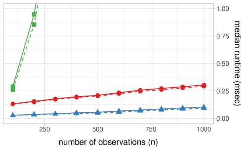
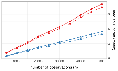
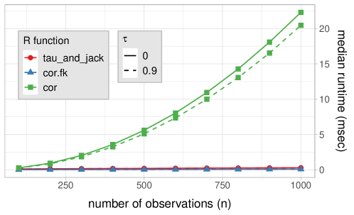
Figure 1: Median runtime of the R functions tau_and_jack (proposed), pcaPP::cor.fk and stats::cor (with method = ‘kendall’) for various sample sizes ($n$) and Kendall correlations ($\tau$) over $1,000$ replications. The data were generated using bivariate Normal distributions.

4 Implementation and benchmarking

We can exploit the result of Section 3 to modify existing $O(n\log_{2}n)$ algorithms for computing $d$ (or $\hat{\tau}$) to return $(d_{1},\dots,d_{n})$ (or $\hat{\tau}$ and $\hat{\sigma}^{2}$) instead. Pseudocode of a merge sort algorithm (see Section 2) is provided in Algorithm A.1 in Appendix; it is loosely based on the C++ code underlying the cor.fk function of the R package pcaPP (Filzmoser et al., , 2018). The general idea is to recursively split $\bm{Y}$ (or suvectors thereof) into two subvectors until these latter are of length less than $10$; these smaller subvectors are then sorted using a so-called insertion sort algorithm (Algorithm A.2) and recursively merged using standard merge sort steps (Algorithm A.3). At each step of the procedure, either in Algorithm A.2 or A.3, a vector variable $\bm{d}$ keeping the swap counts is updated. Note that this also requires keeping track of the position of each component of the original vector $\bm{Y}$ as it is sorted.

We implemented the Algorithms A.1–A.3 in C++ and included them in an R package available on GitHub (see the Supplementary Material for more details). The C++ code is called in a function called tau_and_jack, which computes $\hat{\tau}$ and $\hat{\sigma}^{2}$ in the bivariate case and their natural multivariate extensions $\bm{\hat{\tau}}$ and $\bm{\hat{\Sigma}}$ in higher dimensions. We tested the function in various scenarios by generating datasets of sample sizes $n$ ranging from $100$ to $50,000$. The data was generated using bivariate normal distributions with unit variances and various Pearson’s correlation coefficients $\rho$; for normal distributions $\tau$ is related to $\rho$ by the identity $\tau=(2/\pi)\arcsin\rho$ (Esscher, , 1924). For each scenario considered, we estimated the runtime of tau_and_jack and that of the R functions stats::cor with option method = ‘kendall’ (R Core Team, , 2020) and pcaPP::cor.fk (Filzmoser et al., , 2018), which both compute only $\hat{\tau}$ and not $\hat{\sigma}^{2}$. Based on their implementation, these two should have a runtime of order $n^{2}$ and $n\log_{2}n$, respectively. The experiments were performed on a Dell Precision 5820 machine (Memory: 194GiB, Processor: Intel(R) Xeon(R) W-2145 CPU 3.70GHz $\times$ 16) running the 64-bit operating system Ubuntu 20.04.4 LTS and benchmarked using the microbenchmark package (Mersmann, , 2021).

The results are summarized in Figure 1. They were similar across all values of $\tau$ considered, and so we report only those for $\tau=0$ and $\tau=0.9$. The top panel shows the dependence on $n\in\{100,200,\dots,1000\}$. It suggests that tau_and_jack and cor.fk are much faster than cor when $n$ is large, as expected. The curves corresponding to the two faster functions are shown more clearly in the middle panel of Figure 1, from which we can deduce that they have similar behaviours. In particular, the runtime of both functions appear linear in $n$, with cor.fk being faster by a factor of approximately two for each value of $n$ considered. Further simulations with $5,000\leqslant n\leqslant 50,000$ are shown in the bottom panel of Figure 1; they lead to similar conclusions.

5 Multivariate application

We now use Algorithm A.1 to estimate, via simulations, the finite-sample size and power of one of the tests proposed by Perreault et al., 2022a when $p=50$. More precisely, we consider testing the hypothesis $H_{0}$ that the copula of $\bm{X}=(X_{1},\dots,X_{p})$ is fully exchangeable, i.e., that the distribution $C$ of $\bm{U}=\{F_{1}(X_{1}),\dots,F_{p}(X_{p})\}$ is such that $C(\bm{u})=C\{\pi(\bm{u})\}$ for all permutations $\pi$ of $p$ elements and all $\bm{u}\in[0,1]^{p}$.

It follows from the full exchangeability of $C$ that $\bm{\Sigma}$ contains only three distinct entries, which we denote $(\sigma_{0},\sigma_{1},\sigma_{2})$. The entry of $\bm{\Sigma}$ that corresponds to $\mathbb{C}\mathrm{ov}\{\hat{\tau}(X_{i_{1}},X_{i_{2}}),\hat{\tau}(X_{i_{3}},X_{i_{4}})\}$ is given by $\sigma_{k}$, where $k=|\{i_{1},i_{2}\}\cap\{i_{3},i_{4}\}|$ (Perreault et al., , 2019, Proposition A.1). In such case, a simple strategy for estimating $(\sigma_{0},\sigma_{1},\sigma_{2})$ consists in averaging out their associated entries in $\bm{\hat{\Sigma}}$. We denote by $\bm{\bar{\Sigma}}$ the new estimator of $\bm{\Sigma}$ thus obtained.

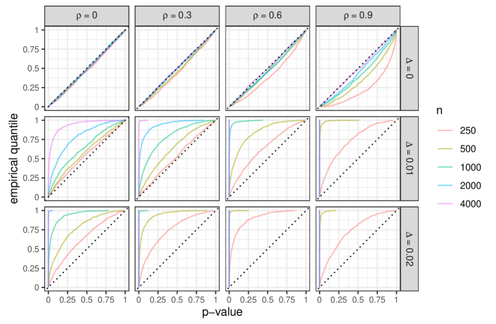
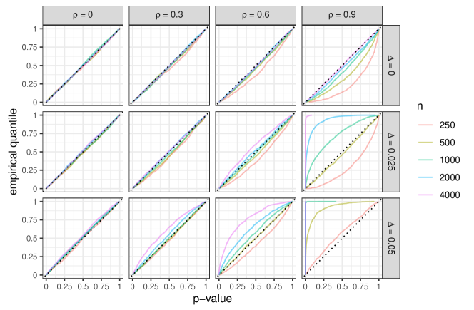
Figure 2: Simulation results ($1000$ replicates) for the test of $H_{0}$ under check departures. The obtained p-values are plotted against their corresponding empirical quantile.

In what follows, we use Proposition D.1 of Perreault et al., 2022b to estimate $(\sigma_{0},\sigma_{1},\sigma_{2})$ directly from $\bm{\hat{g}}_{1},\dots,\bm{\hat{g}}_{n}$, so that $\bm{\hat{\Sigma}}$ is never actually stored in its entirety. We test $H_{0}$ with the statistic $E:=\|\bm{\bar{\Sigma}}^{-1/2}(\bm{\hat{\tau}}-\bm{\bar{\tau}})\|_{2}^{2}$, where $\bm{\bar{\tau}}$ is the $\binom{p}{2}$-dimensional vector that repeats the average of the elements of $\bm{\hat{\tau}}$. Following Proposition 5.1 of Perreault et al., 2022a , we compute a p-value by comparing $E$ to the quantiles of a $\chi_{r}$ distribution, where $r=\binom{p}{2}-1=1224$. Note that $\bm{\bar{\Sigma}}$ need not be explicitely constructed for performing the test.

To approximate the size and power of the the test based on $E$, we generate datasets of dimensions $n\times 50$ for various values of $n$ (specified below) using a Normal distribution with unit variances. Under the null, the $50\times 50$ correlation matrix $\bm{R}$ of $\bm{X}$ is of the form $\bm{R}=(1-\rho)\bm{I}+\rho\bm{J}$, where $\bm{J}$ is a matrix of ones and $\rho\in(0,1)$. We define three types of departures from the null in terms correlation matrices: single ($\bm{R}^{\prime}$), column ($\bm{R}^{\dagger}$) and check ($\bm{R}^{\#}$) departures. More precisely, for $i,j\in\{1,\dots,50\}$, we let

$$R_{ij}^{\prime}=R_{ij}+\Delta\times\mathbbm{1}(\{i,j\}=\{1,2\})\;,\qquad R_{ij}^{\dagger}=R_{ij}+\Delta\times\mathbbm{1}(1\not\in\{i,j\})$$

and

$$R_{ij}^{\#}=R_{ij}+\Delta\times\mathbbm{1}(i+j\text{ is odd})$$

for some $\Delta\in[0,1-\rho)$. Note that only the single and column departures were considered in the simulation study of Perreault et al., 2022a ; the simulation results for check departures are new.

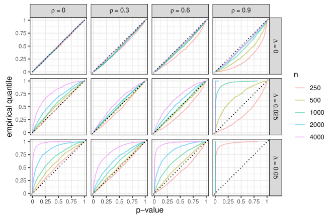
We repeated the experiment $1000$ times for each combination of departure (single, column, check), sample size $n\in\{250\cdot 2^{i}:0\leqslant i\leqslant 4\}$, dependence parameter $\rho\in\{0,.3,.6,.9\}$ and departure strength $\Delta\in\{0,0.025,0.05\}$. To present more meaningful results, we further considered check departures of strength $\Delta\in\{0.01,0.02\}$. The results for single and column departures, summarized in Appendix B in Figures B.1 and B.2, respectively, are consistent with the findings of Perreault et al., 2022a . We thus focus on the results for check departures (with $\Delta\in\{0,0.01,0.02\}$), which are summarized in Figure 2.

They suggest that $n=250$ observations is enough to obtain reasonable sizes when $\rho\in\{0,0.3,0.6\}$, but that more data are required as $\rho$ further approaches $1$. Despite some very conservative sizes, the tests are able to detect check departures quite well for the values of $\Delta$ tested. In particular, when $n=250$ and $\rho=0.9$, the test performed at nominal level $\alpha=0.05$ has an estimated size ($\Delta=0$) of $1.2\%$, while its estimated power is as much as $97.4\%$ when $\Delta=0.02$. Although the results for different types of departures should not be directly compared (even for an identical value of $\Delta$), it seems fair to say that check departures are more easily detected by the test than single and column departures.

On the computer described in Section 4 and with $\rho=\Delta=0$, performing one test takes ${\sim}75$, ${\sim}165$ and ${\sim}1,456$ msec for samples of size $n=250,500$ and $4000$, respectively. For comparison, the test procedure used by Perreault et al., 2022a , which explicitely computes $\hat{\sigma}^{2}$ in (3) as a double sum involving $O(n^{2})$ comparisons, takes ${\sim}1,958$ and ${\sim}8,568$ msec when $n=250$ and $500$, respectively.

6 Summary and potential improvement

In this paper, it is explained how the well-known algorithm of Knight, (1966) can be modified to compute both Kendall’s $\hat{\tau}$ and a jackknife estimate of its variance. Given a dataset $\{(X_{i},Y_{i})\}_{i=1}^{n}$ of $n$ observations for which $X_{1}<\dots<X_{n}$, Knight’s (1966) method for computing $\hat{\tau}$ relies on counting the number of swaps required to sort $(Y_{1},\dots,Y_{n})$ using exchange sort. The proposed algorithm consists in recording not the total number of swaps, but the number of times each observation is swapped.

Throughout the paper, however, it is assumed that the random variables under study are continuous, and hence that there is almost surely no ties among the observations. On this aspect, the proposed algorithm is less general than that of Knight, (1966). An extension accounting for ties would significantly improve the applicability of the method. Interesting recent advances about inference for Kendall’s $\tau$ when there are ties among the observations can be found in Nowak and Konietschke, (2021).

Appendix A Algorithms

Algorithm A.1 Merge sort algorithm keeping the swap counts.

1:$\bm{y},\bm{x}$: numeric vectors of length $m,m$. $\triangleright$ observations and storage

2:$\bm{q},\bm{p},\bm{d}$: are integer vectors of length $m,m,n$. $\triangleright$ ids, storage and swap counts

3:*This function is recursive. It is assumed that, in total, $n$ observations $(y_{1},\dots,y_{n})$ are available and that $m=n$ when the procedure is first called and $m\leqslant n$ in general; $\bm{q}$ can be initialized with $(1,\dots,n)$ or any permutation of it; $\bm{d}$ is initialized with $n$ zeros.

4:

5:procedure MergeSort($\bm{y},\bm{x},\bm{q},\bm{p},\bm{d}$)

6:     if $m<10$ then

7:         do InsertionSort($\bm{y},\bm{q},\bm{d}$)

8:     else

9:         do MergeSort($\bm{y}^{\prime},\bm{x}^{\prime},\bm{q}^{\prime},\bm{p}^{\prime},\bm{d}$) $\triangleright$ $\bm{z}^{\prime}=(z_{1},\dots,z_{\lfloor m/2\rfloor})$

10:         do MergeSort($\bm{y}^{*},\bm{x}^{*},\bm{q}^{*},\bm{p}^{*},\bm{d}$) $\triangleright$ $\bm{z}^{*}=(z_{\lfloor m/2\rfloor+1},\dots,z_{m})$

11:         do MergeSortStep($\bm{y},\bm{x},\bm{q},\bm{p},\bm{d}$)      

12:     $\bm{y}$ $\leftarrow$ $\bm{x}$

Algorithm A.2 Insertion sort algorithm keeping the swap counts.

1:$\bm{y}$: numeric vector of length $m$. $\triangleright$ observations

2:$\bm{q},\bm{d}$: integer vectors of length $m,m,n$. $\triangleright$ ids and swap counts

3:($m\leqslant n$, $\bm{q}$ is a subvector of $(1,\dots,n)$)

4:

5:procedure InsertionSort($\bm{y},\bm{q}$, $\bm{d}$)

6:     for $i\leftarrow(m-1)\textrm{ to }1$ do

7:         $z$ $\leftarrow$ $y_{i}$

8:         $\ell$ $\leftarrow$ $q_{i}$

9:         $j$ $\leftarrow$ $i$

10:         while $y_{j+1}<z$ and $j<m$ do

11:              $y_{j}$ $\leftarrow$ $y_{j+1}$

12:              $q_{j}$ $\leftarrow$ $q_{j+1}$

13:              $d_{q_{j+1}}$ $\leftarrow$ $d_{q_{j+1}}+1$

14:              $j$ $\leftarrow$ $j+1$          

15:         $y_{j}$ $\leftarrow$ $z$

16:         $q_{j}$ $\leftarrow$ $\ell$

17:         $d_{q_{j}}$ $\leftarrow$ $d_{q_{j}}+(j-i)$      

Algorithm A.3 Single step of a merge sort algorithm keeping the swap counts.

1:$\bm{y},\bm{x}$: numeric vectors of length $m,m$. $\triangleright$ observations and storage

2:$\bm{q},\bm{p},\bm{d}$: integer vectors of length $m,m,n$. $\triangleright$ ids, storage and swap counts

3:($1<m\leqslant n$, $\bm{q}$ is a subvector of $(1,\dots,n)$)

4:

5:procedure MergeSortStep($\bm{y},\bm{x},\bm{q},\bm{p},\bm{d}$)

6:     $m^{\prime}$ $\leftarrow$ $\lfloor m/2\rfloor$

7:     $m^{*}$ $\leftarrow$ $m-m^{\prime}$

8:     $i,j$ $\leftarrow$ $1$

9:     while $i\leqslant m^{\prime}\textrm{ and }j\leqslant m^{*}$ do

10:         if $y_{i}<y_{m^{\prime}+j}$ then

11:              $x_{i+j}$ $\leftarrow$ $y_{m^{\prime}+j}$

12:              $p_{i+j}$ $\leftarrow$ $q_{m^{\prime}+j}$

13:              $d_{q_{m^{\prime}+j}}$ $\leftarrow$ $d_{q_{m^{\prime}+j}}+(m^{\prime}-i+1)$

14:              $j$ $\leftarrow$ $j+1$

15:         else

16:              $x_{i+j}$ $\leftarrow$ $y_{i}$

17:              $p_{i+j}$ $\leftarrow$ $q_{i}$

18:              $d_{q_{i}}$ $\leftarrow$ $d_{q_{i}}+(j+1)$

19:              $i$ $\leftarrow$ $i+1$               

20:     if $i<m^{\prime}$ then

21:         $(x_{i},\dots,x_{m^{\prime}})$ $\leftarrow$ $(y_{i},\dots,y_{m^{\prime}})$

22:         $(p_{i},\dots,p_{m^{\prime}})$ $\leftarrow$ $(q_{i},\dots,q_{m^{\prime}})$

23:         $(d_{q_{i}},\dots,d_{q_{m^{\prime}}})$ $\leftarrow$ $(d_{q_{i}},\dots,d_{q_{m^{\prime}}})+m^{*}$

24:     else

25:         $(x_{m^{\prime}+j},\dots,x_{m})$ $\leftarrow$ $(y_{m^{\prime}+j},\dots,y_{m})$

26:         $(p_{m^{\prime}+j},\dots,p_{m})$ $\leftarrow$ $(q_{m^{\prime}+j},\dots,q_{m})$      

Appendix B Simulations results for single and column departures

Figure B.1: Simulation results ($1000$ replicates) for the test of $H_{0}$ under single departures. The obtained p-values are plotted against their corresponding empirical quantile.

Figure B.2: Simulation results ($1000$ replicates) for the test of $H_{0}$ under column departures. The obtained p-values are plotted against their corresponding empirical quantile.

References

• Abrevaya, (1999) Abrevaya, J. (1999). Computation of the maximum rank correlation estimator. Econ. Lett., 62:279–285.
• Bergsma and Dassios, (2014) Bergsma, W. and Dassios, A. (2014). A consistent test of independence based on a sign covariance related to Kendall’s tau. Bernoulli, 20:1006–1028.
• Chen, (2018) Chen, X. (2018). Gaussian and bootstrap approximations for high-dimensional U-statistics and their applications. Ann. Statist., 46:642–678.
• Christensen, (2005) Christensen, D. (2005). Fast algorithms for the calculation of Kendall’s τ𝜏\tau. Comput. Stat., 20:51–62.
• Cormen et al., (2014) Cormen, T. H., Leiserson, C. E., Rivest, R. L., and Stein, C. (2014). Introduction to Algorithms. MIT press, 4th edition.
• Esscher, (1924) Esscher, F. (1924). On a method of determining correlation from the ranks of the variates. Scand. Actuar. J., 1924:201–219.
• Filzmoser et al., (2018) Filzmoser, P., Fritz, H., and Kalcher, K. (2018). pcaPP: Robust PCA by Projection Pursuit. R package version 1.9-73.
• Genest et al., (2011) Genest, C., Nešlehová, J., and Ben Ghorbal, N. (2011). Estimators based on Kendall’s tau in multivariate copula models. Aust. N. Z. J. Stat., 53:157–177.
• Hájek, (1968) Hájek, J. (1968). Asymptotic normality of simple linear rank statistics under alternatives. Ann. Math. Statist., 39:325–346.
• Hamed, (2011) Hamed, K. H. (2011). The distribution of Kendall’s tau for testing the significance of cross-correlation in persistent data. Hydrol. Sci. J., 56:841–853.
• Hoeffding, (1948) Hoeffding, W. (1948). A class of statistics with asymptotically normal distribution. Ann. Math. Statist., 19:293–325.
• Kendall, (1948) Kendall, M. G. (1948). Rank Correlation Methods. Griffin.
• Knight, (1966) Knight, W. R. (1966). A computer method for calculating Kendall’s tau with ungrouped data. J. Am. Stat. Assoc., 61:436–439.
• Knuth, (1998) Knuth, D. (1998). The Art of Computer Programming: Volume 3: Sorting and Searching. Addison-Wesley.
• Lakhal et al., (2008) Lakhal, L., Rivest, L.-P., and Abdous, B. (2008). Estimating survival and association in a semicompeting risks model. Biometrics, 64:180–188.
• Lebrenz and Bárdossy, (2017) Lebrenz, H. and Bárdossy, A. (2017). Estimation of the variogram using Kendall’s tau for a robust geostatistical interpolation. J. Hydrol. Eng., 22:04017038.
• Leung and Drton, (2018) Leung, D. and Drton, M. (2018). Testing independence in high dimensions with sums of rank correlations. Ann. Statist., 46:280–307.
• Mao, (2018) Mao, G. (2018). Testing independence in high dimensions using Kendall’s tau. Comput. Statist. Data Anal., 117:128–137.
• Martin and Betensky, (2005) Martin, E. C. and Betensky, R. A. (2005). Testing quasi-independence of failure and truncation times via conditional Kendall’s tau. J. Am. Stat. Assoc., 100:484–492.
• McNeil et al., (2015) McNeil, A. J., Frey, R., and Embrechts, P. (2015). Quantitative Risk Management. Princeton University Press, revised edition.
• Mersmann, (2021) Mersmann, O. (2021). microbenchmark: Accurate Timing Functions. R package version 1.4.9.
• Nelsen, (2006) Nelsen, R. B. (2006). An Introduction to Copulas. Springer, 2nd edition.
• Nowak and Konietschke, (2021) Nowak, C. P. and Konietschke, F. (2021). Simultaneous inference for Kendall’s tau. J. Multivar. Anal., 185:104767.
• Perreault et al., (2019) Perreault, S., Duchesne, T., and Nešlehová, J. G. (2019). Detection of block-exchangeable structure in large-scale correlation matrices. J. Multivar. Anal., 169:400–422.
• (25) Perreault, S., Nešlehová, J. G., and Duchesne, T. (2022+a). Hypothesis tests for structured rank correlation matrices. Under review.
• (26) Perreault, S., Nešlehová, J. G., and Duchesne, T. (2022+b). Hypothesis tests for structured rank correlation matrices (supplementary material). Under review.
• R Core Team, (2020) R Core Team (2020). R: A Language and Environment for Statistical Computing. R Foundation for Statistical Computing.
• Rublík, (2016) Rublík, F. (2016). Estimates of the covariance matrix of vectors of u-statistics and confidence regions for vectors of Kendall’s tau. Kybernetika, 52:280–293.
• van der Vaart, (1998) van der Vaart, A. W. (1998). Asymptotic Statistics. Cambridge University Press.