Finding and Following Optimal Trajectories for an Overactuated Floating Robotic Platform

Abstract

The recent increase in yearly spacecraft launches and the high number of planned launches have raised questions about maintaining accessibility to space for all interested parties. A key to sustaining the future of space-flight is the ability to service malfunctioning - and actively remove dysfunctional spacecraft from orbit. Robotic platforms that autonomously perform these tasks are a topic of ongoing research and thus must undergo thorough testing before launch. For representative system-level testing, the European Space Agency (ESA) uses, among other things, the Orbital Robotics and GNC Lab (ORGL), a flat-floor facility where air-bearing based platforms exhibit free-floating behavior in three Degrees of Freedom (DoF). This work introduces a representative simulation of a free-floating platform in the testing environment and a software framework for controller development. Finally, this work proposes a controller within that framework for finding and following optimal trajectories between arbitrary states, which is evaluated in simulation and reality.

1 INTRODUCTION

Space debris is widely recognized as a significant problem for safely operating spacecraft in orbit [1, 2, 3, 4]. Especially the popular orbits experience more usage and are slowly becoming crowded. Despite extensive requirements for ensuring a safe de-orbit of a satellite some spacecraft and debris already are and will remain in orbit indefinitely. Many experts in the community argue that Active Space Debris Removal (ASDR) will play a key role in maintaining accessibility to these popular orbits [5, 6, 7]. Automatic robotic systems for ASDR are topic of ongoing research and thus require stringent testing on a full system level before launch. At the cost of reducing the system to three DoF, air-bearing platforms on flat-floors provide a representative environment to test technologies in the free-floating domain, which is otherwise difficult to emulate. Such a facility is present at ESTEC, an ESA facility. The ORGL, as described in detail in [8, 9], consists of a $5\text{\times}9\text{\,}\mathrm{m}$ epoxy flat-floor and houses multiple floating platforms. The floating platforms functions are twofold: Firstly, it functions as a target for testing new technologies in ASDR. Secondly, it provides a base for tested modules that are mounted on top of the stack and thus are tested independently of the basic motion.

This works has two main contributions. Firstly it introduces a high-fidelity simulation and visualization of a generic floating platform that resembles the floating platform at the ORGL using the robotics simulator Gazebo [10]. Secondly, this work proposes a modular control architecture for floating platforms equipped with binary thrusters and a Reaction-Wheel (RW).

The remainder of this work is structured as follows: first, section 2 introduces a system model. Afterwards section 3 explains the developed simulation before section 4 explains the control framework and showcases it on an example of an optimal trajectory finding and tracking controller. Finally, section 5 summarizes the results and gives an outlook on future work.

2 SYSTEM DESCRIPTION

One of the floating platforms within the ORGL, consists of a modular stack that resembles a realistic satellite actuator assembly. In the following this work first describes the used hardware and then continues to introduce the dynamic model used to approximate the overall system.

2.1 Hardware

The floating platform consists of three modules as depicted in Figure 1. They each serve an individual function:

• Air Cushion Robotic Platform (ACROBAT) is equipped with three air-bearings and provides a floating base.

• Satellite Simulator (SATSIM) is equipped with four pairs of counter-facing, radially aligned, solenoid-valve-based thrusters. Each provides approximately $\bar{f}=$10\text{\,}\mathrm{N}$$ of thrust. Further it houses two compressed air tanks that function as the propellant storage.

• Reaction Control Autonomy Platform (RECAP) is a RW and provides a torque on the system.

When mounted together they form the full floating platform. Table 1 shows the inertial parameters of the individual modules and the overall system.

Table 1: Mass, MoI and size properties of the subsystems and the overall sum.

Subsystem	Mass	MoI	Height	Radius
ACROBAT	$154\text{\,}\mathrm{kg}$	$10.090\text{\,}\mathrm{k}\mathrm{g}\mathrm{m}^{2}$	$62.5\text{\,}\mathrm{cm}$	$35\text{\,}\mathrm{cm}$
SATSIM	$50\text{\,}\mathrm{kg}$	$1.416\text{\,}\mathrm{k}\mathrm{g}\mathrm{m}^{2}$	$20\text{\,}\mathrm{cm}$	$35\text{\,}\mathrm{cm}$
RECAP	$13.66\text{\,}\mathrm{kg}$	$0.67\text{\,}\mathrm{k}\mathrm{g}\mathrm{m}^{2}$	$20\text{\,}\mathrm{cm}$	$35\text{\,}\mathrm{cm}$
RW	$4.01\text{\,}\mathrm{kg}$	$0.047\text{\,}\mathrm{k}\mathrm{g}\mathrm{m}^{2}$	–	–
$\Sigma$	$221.67\text{\,}\mathrm{kg}$	$12.223\text{\,}\mathrm{k}\mathrm{g}\mathrm{m}^{2}$	$102.5\text{\,}\mathrm{cm}$	–

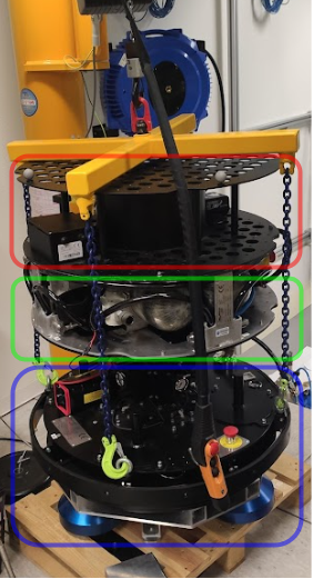
Figure 1: The modular floating platform stack consisting of the three modules ACROBAT (blue), SATSIM (green) and RECAP (red) – the floating base, thruster assembly and RW respectively. The stack is pictured in its mounting crane used to hoist it on the flat-floor.

2.2 Dynamic Model

This work models the system as an assembly of perfect geometry shapes, which are denoted as links. Links are connected via different joints and forces and torques (wrenches) act on individual joints or links.

As depicted in Figure 2, the model consists of a large cylinder, representing the main chassis, eight small rectangular boxes, representing the eight thrusters, and a smaller cylinder representing the RW. The thrusters are connected via fixed joints whereas the RW connects to the main chassis via a revolut joint.

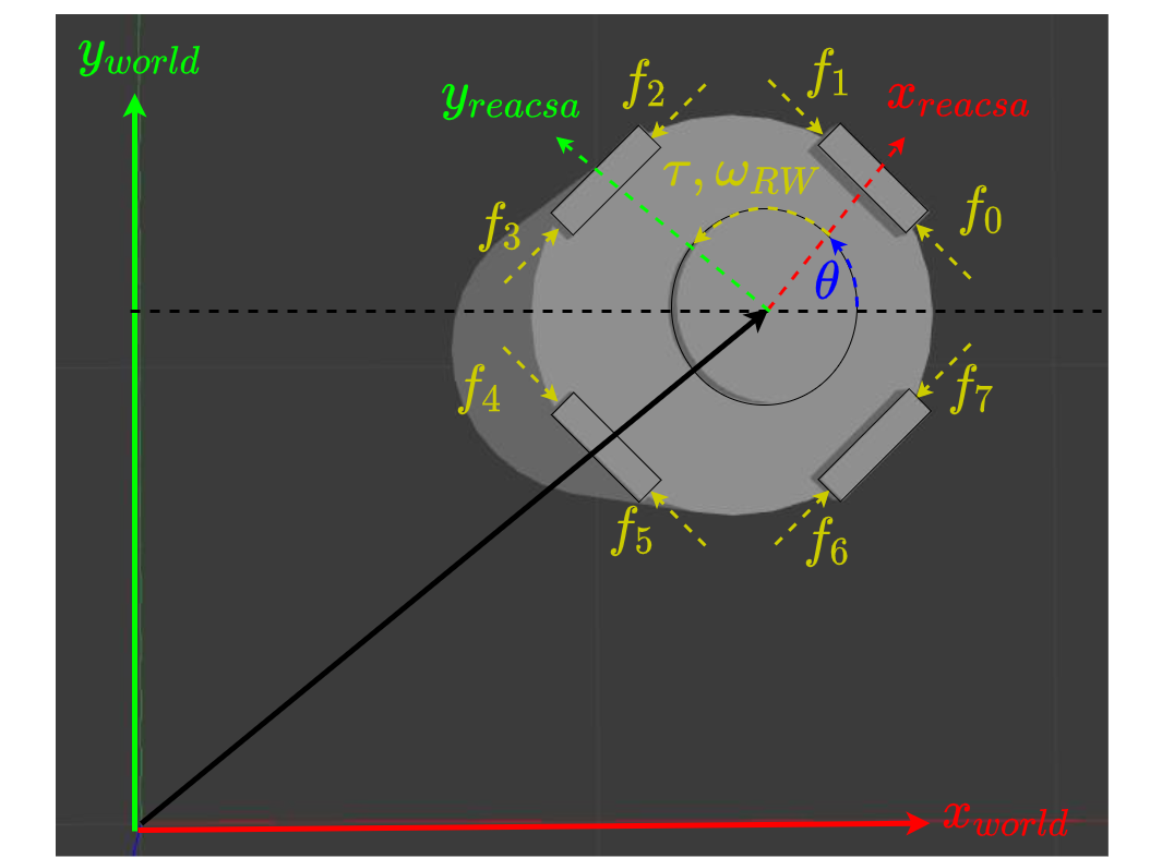
Figure 2: Definitions of coordinate systems and wrenches supplied by the actuators. The position of the system is defined in some world coordinate system and the orientation as the angle between the world coordinate system and the local coordinate system. The torque $\tau$ and the RW velocity $\omega_{RW}$ are defined in mathematical positive direction and the forces for all individual thrusters are also numbered in mathematically positive direction. Naturally, counting starts at zero.

This work denotes the forces produced by the thrusters at the $i$-th instance as $f_{i}$ attacking at the origin of the rectangular box link, and the torque the motor produces on the revolut joint that connects the RW as $\tau$. Since the thrusters are solenoid valves they only allow for the states on and off, i.e. $f_{i}\in\{0,\bar{f}\}\;\;\forall i\in[0,7]$. Thus, the control vector $\bm{u}$ consists of the eight forces by the thrusters and the torque on the RW:

$$\bm{u}=\begin{bmatrix}\tau&f_{0}&f_{1}&f_{2}&f_{3}&f_{4}&f_{5}&f_{6}&f_{7}\end{bmatrix}^{T}\;.$$ (1)

The following state vector $\bm{x}$ describes the system state when moving along the three DoF:

$$\bm{x}=\begin{bmatrix}x&y&\theta&\dot{x}&\dot{y}&\dot{\theta}&\omega_{RW}\end{bmatrix}^{T}\;,$$ (2)

where $x,y,\theta$ describe the system position and orientation with respect to the world coordinate system and $\omega_{RW}$ describes the current angular velocity of the RW.

Assuming a perfectly flat floor and zero friction between the main chassis and the floor the resulting state equation is:

(3)

where $s_{\theta}$ and $c_{\theta}$ denote the sine and cosine of the respective angle, $m$ is the system mass, $I_{w}$ and $I_{b}$ are the MoI of the RW and the overall system respectively, and $\bm{w}$ incorporates all external disturbances. Note that each coordinate individually exhibits simple double integrator behavior.

The system pose is measured via a global Motion-Capture (MoCap) system and the current RW velocity via a motor encoder. Thus the output matrix of the state space system is identity and noise $\bm{v}$ is assumed to be Additive White Gaussian Noise (AWGN):

$$\bm{y}=\bm{I}\bm{x}+\bm{v}\;.$$ (4)

3 SIMULATION

This section introduces the simulation used to emulate the dynamic model described in section 2.2. This allows for faster and safer prototyping before testing on the physical hardware. To increase the transferability of the results from simulation to the physical system some real-world approximations are incorporated.

3.1 Sensor Noise

In any physical system sensors are subject to noise. As captured by the measurement equation (4), this work assumes the noise to be AWGN. I.e. in the simulation a term drawn from the zero-mean, two dimensional Gaussian distributions, with the standard deviations $\sigma_{position}$, $\sigma_{velocity}$ is added to the $(x,y)$ position and $(\dot{x},\dot{y})$ velocity before publishing. The same is done for the angular velocity $\dot{\theta}$ with a standard deviation $\sigma_{ang-velocity}$. Since the orientation $\theta$ is not in euclidean space the sensor noise cannot directly be added. Instead a noise angle is drawn from a zero-mean Gaussian distribution with standard deviation $\sigma_{angle}$ and the equivalent unit quaternion is computed. The true pose is then multiplied with this noise quaternion before publishing the resulting noisy orientation.

3.2 Uneven Floor

The flat-floor at the ORGL is one of the flattest of its kind, however, the small slopes that exist on the floor are enough to introduce significant disturbances into the system. The simulation models this unevenness in Gazebo using a Digital Elevation Model (DEM). In particular, the measurements from [8] provide the base for the DEM. Gazebo natively supports the creation of DEM from a gray-scale png image. It requires the image to be quadratic and the resolution to be of the form $2^{N}+1\text{ where }N\in\mathds{N}_{0}^{+}$. Hence, to strike a balance between resolution and computational complexity the height-map is chosen to be of resolution $513\text{\times}513\text{\,}\mathrm{p}\mathrm{x}$, which is equivalent to approximately $2\text{\,}\mathrm{c}\mathrm{m}\mathrm{/}\mathrm{p}\mathrm{x}$. Figure 3 shows the resulting height-map.

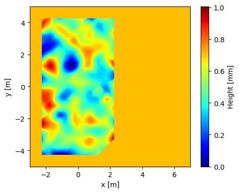
Figure 3: Height-map used to simulate the unevenness of the flat-floor. Blue colors imply low regions and red colors high regions. All regions outside the main flat-floor are set to some arbitrary medium height.

4 CONTROL

For each controller one has to make choices on design and architecture. With the goal of modularity and the constraints of the system in mind this section first introduces the modular control architecture and then continues to showcase a specific implementation.

4.1 Architecture

The architecture consists of two main building blocks: a trajectory planner that pre-computes optimal trajectories and a trajectory tracker that follows those trajectories. The problem of finding optimal binary control actions is of the problem class Mixed-Integer Non-Linear Programming (MINLP) which are considered computationally intractable, even for smaller dimensional state-spaces [11]. Thus, this work proposes to use a simplified model that relaxes the binary condition on the thrusters for the planner and parts of the tracker. These continuous control values are then translated on the binary thrusters using some modulation scheme. Thus, the tracker consists of a feedback controller that computes controls of the simplified model online, a modulator that translates the continuous control onto the binary thrusters and an observer that estimates the current system state using the most recent measurements and binary control actions. Figure 4 visualizes this overall structure.

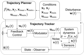
Figure 4: The basic building blocks of the control framework: a trajectory planner that pre-computes trajectories, and a trajectory tracker that follows the trajectories.

The software used in this work realizes the controller in Robot-Operating-System 2 (ROS2) [12]. Hence, each module and sub-module represents an individual node that communicates via topics, services, and actions. In particular, each module can be replaced by a different version that implements the respective interface and publishes to the correct topics.

4.2 Finding and Following Optimal Trajectories

Using this architecture this work showcases a controller that pre-computes trajectories that minimize the force applied by the thrusters and follows them.

Control Law

The optimal trajectories are computed for the simplified system in which the thrusters can provide continuous force. In this simplified system the problem of finding an optimal trajectory that minimize the quadratic actuation, weighted by some matrix $\bm{R}$, is equivalent to solving a quadratic program as described in [13]. The resulting optimization problem over all states $\bm{X}$ and control values $\bm{U}$ at all knot-points $k\in[1,N]$ is:

$$\begin{aligned} &\min_{\bm{X},\bm{U}}\left\{\sum_{k=1}^{N}\bm{u}_{k}\bm{R}\bm{u}_{k}^{T}\right\}\;\;\;\forall k\in[1,N-1]\text{ s.t. }\\ &\;\;\;\;\bm{x}(0)=\bm{x}_{init},\;\;\;\bm{x}(t_{f})=\bm{x}_{final}\\ &\;\;\;\;\bm{x}_{min}\leq\bm{x}_{k}\leq\bm{x}_{max},\quad\bm{u}_{min}\leq\bm{u}_{k}\leq\bm{u}_{max}\\ &\;\;\;\;\bm{x}_{k+1}-\bm{x}_{k}=\frac{\Delta t}{6}(\bm{f}_{k}+4\bm{f}_{k+1/2}+\bm{f}_{k+1})\\ &\text{where }\\ &\;\;\;\;\bm{x}_{k+1/2}=\frac{1}{2}(\bm{x}_{k}+\bm{x}_{k+1})+\frac{\Delta t}{8}(\bm{f}_{k}-\bm{f}_{k+1})\\ &\;\;\;\;\bm{u}_{k+1/2}=\frac{1}{2}(\bm{u}_{k}+\bm{u}_{k+1})\\ \end{aligned}$$ (5)

In particular, the system state and control action are discretized along time at $N$ knot points where the first and last correspond to the starting and the desired final state. The state as well as the control action are subject to linear bounding box constraints and the system dynamics, i.e. at each knot point the state and control action must yield the next state when propagated through the system dynamics as in equation (3), while not exceeding the state and control limits. Direct collocation [14] (Hermite-Simpson) is chosen as the transcription method.

The optimization problem is solved offline using the programming interface “Drake” [15] to the open source solver “IPOPT” [16]. To compute the continuous online control to follow the trajectory this work uses a Time-Varying Linear Quadratic Regulator (TVLQR) as introduced in [17]. The continuous control is further fed to the modulator, which is implemented as a $\Sigma\Delta$-Modulator as in [18]. Finally, the system state is estimated using a classic Kalman Filter [19].

Results

The previously introduced controller is tested in simulation, on a perfectly flat floor and on a floor described by the DEM, as well as on the physical system. In simulation the tested trajectory is a set of 40 states where each lies on a circle of radius $0.5\text{\,}\mathrm{m}$ with a constant tangential velocity. Between each consecutive pair of states the trajectory planner finds an optimal trajectory. Figure 5 shows the resulting position, velocity and required continuous actuation.

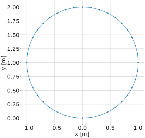
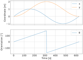
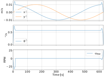
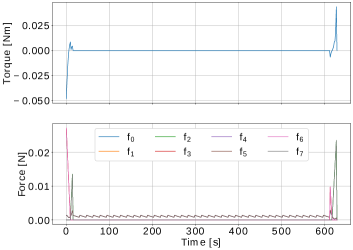
Figure 5: The optimal, pre-computed circular trajectory. Each dot in the ground-track (top graph) represents one state (position on the circle, constant tangential velocity), in between which the trajectory planner computes an optimal trajectory.

Figure 6 shows the simulated results. As displayed qualitatively by the groundtrack the system follows the desired trajectories in simulation with a small error. Table 2 displays the average errors along the trajectory and confirms this quantitatively. On the perfectly flat floor the average euclidean error stays below $3.5\text{\,}\mathrm{cm}$ and the angular error below $5\text{\,}\mathrm{\SIUnitSymbolDegree}$. The average euclidean error approximately doubles for the uneven floor but remains below $8\text{\,}\mathrm{cm}$ and the average angular error remains the same. The average angular error is similar for both cases because the system model has a single-cylinder as the main chassis, which only experiences disturbance forces due to the uneven floor. However, it experiences no disturbance torques since the cylinder has a single contact to the uneven floor.

	Simulated Circular		Physical
	Without DEM	With DEM	Straight-Line	Semi-Circle
$e_{x}$	$0.0238\text{\,}\mathrm{m}$	$0.0566\text{\,}\mathrm{m}$	$0.256\text{\,}\mathrm{m}$	$0.317\text{\,}\mathrm{m}$
$e_{y}$	$0.0224\text{\,}\mathrm{m}$	$0.0506\text{\,}\mathrm{m}$	$0.200\text{\,}\mathrm{m}$	$0.311\text{\,}\mathrm{m}$
$e_{|x,y|}$	$0.0327\text{\,}\mathrm{m}$	$0.0759\text{\,}\mathrm{m}$	$0.325\text{\,}\mathrm{m}$	$0.444\text{\,}\mathrm{m}$
$e_{\theta}$	$4.52\text{\,}\mathrm{\SIUnitSymbolDegree}$	$4.36\text{\,}\mathrm{\SIUnitSymbolDegree}$	$23.8\text{\,}\mathrm{\SIUnitSymbolDegree}$	$51.2\text{\,}\mathrm{\SIUnitSymbolDegree}$

Table 2: The average error of the system trying to follow trajectories (simulated and on the physical system) for the individual coordinates and the euclidean distance. Both cases, with and without an DEM, are shown. The error is computed from the desired trajectory and the ground-truth pose obtained from the simulation.

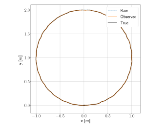
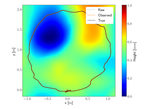
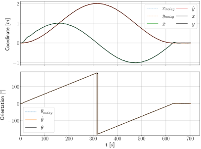
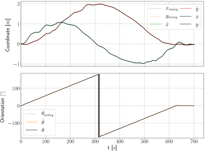
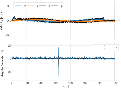
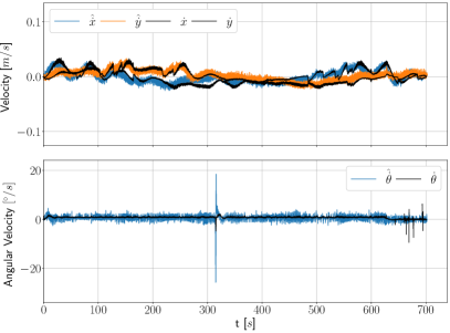
Figure 6: Ground-track, individual coordinates, and velocity of the system following a circular trajectory in simulation. Left: ideally even floor. Right: the floor is slightly uneven and induces disturbances. An animation of the trajectory is given at https://youtu.be/1A5xJVEAU9w?t=42.

On the physical system the controller is tested by following an optimal straight line trajectory connecting two zero velocity states and a semi-circle (half of the simulated trajectory). Figure 7 and 8 show the results on the physical system.

Compared to the previous, simulated results the performance significantly decreases, increasing the average euclidean error by approximately an order of magnitude (cf. table 2). For the straight-line trajectory the largest error occurs along the x-axis. This is due to the slope of the ground introducing larger disturbance along that direction. In particular the region between the local maximum at $(1.75,1.5)$ and the minimum at $(0.5,1.5)$ (cf. Figure 3) imposes a significant acceleration. Thus, the controller remains in an equilibrium distance to the trajectory where the cost of actuation is equivalent to the penalty due to the pose error. Furthermore, in both trajectories the RW saturates on both ends of the allowable range as depicted in Figure 8. At each instance a larger deviation from the desired orientation is observed which implies that large desired changes in angular momentum of the entire system quickly lead to RW saturation. For the semi-circle the effect is even more significant. Once the RW saturates the system starts oscillating about the desired orientation, falling into a large limit cycle of the orientation control using the thrusters. The average euclidean distance to the desired semi-circle is $0.444\text{\,}\mathrm{m}$ and the angular error is $51.2\text{\,}\mathrm{\SIUnitSymbolDegree}$. Within the semi-circle trajectory one particular downside of the a-priori planning approach is displayed. The system slides down a steep slope (approximately at the local blue minimum at $(0,2)$) and gets ahead of the trajectory. Since the trajectory follower does not recompute the planned trajectory and only attempts to move the system to a currently desired state, it returns to a previous location. It then follows the trajectory, resulting in a loop in the ground-track. However, as shown by the groundtracks, the general shape of the desired trajectories remains consistent. Further, as displayed by Figure 8 the thruster usage is of low frequency, never exceeding the one-and two fire per second threshold for the straight line and the semi-circle respectively.

The major decrease from the simulation to the physical system is attributed to two main factors: errors in the system model and lack of control authority. The controller would especially benefit from a full system identification in terms of inertial parameters and individual thrust vector determination for each thruster. Moreover, given the large weight of the system and the comparably low force capabilities by the thrusters, high actuation is required to compensate even small disturbances induced by the unevenness of the flat-floor.

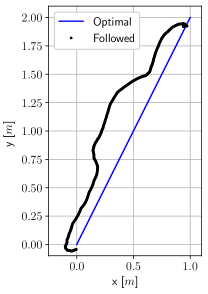
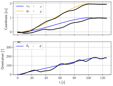
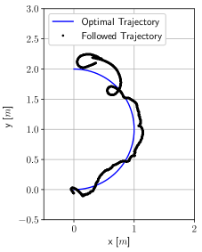
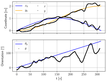
Figure 7: Ground-track and individual coordinates of the controller following a straight-line trajectory (top row) and a semi-circular trajectory (bottom row) on the real system. After reaching the final pose of the trajectory plots (right) in the coordinate plots, the desired value is indicated as a dashed line. Videos of the trajectories are given at https://youtu.be/1A5xJVEAU9w?t=243

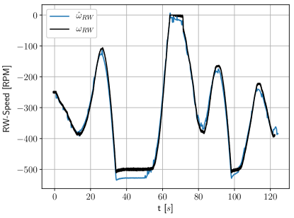
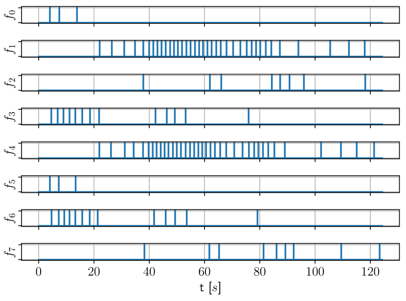
(a)

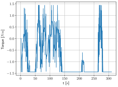
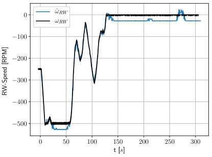
(b)

Figure 8: Actuation of following trajectories on the physical system (cf. Figure 7). Figure 8(a) shows the actuation for the straight line, Figure 8(b) for the semi-circle. For both the top left shows the torque exerted by the motor onto the RW, the top right the resulting RW velocity (raw and observed), and the bottom the thruster activity for all eight thrusters.

5 SUMMARY

For system-level testing of spacecraft a flat-floor in combination with air-bearing based platforms provide a representative setup for development and validation. At the ESA the ORGL takes on this role. This work introduces a simulation, developed with ROS2 and Gazebo, of the floating platform within the ORGL at the ESA. The simulation uses an approximate model of the floating platform and takes the small unevenness of the flat-floor as well as sensor noise into account to model and visualize trajectories of the system. This allows for pre-validation and testing of newly developed algorithms in software before testing it in hardware. Further, this work introduces an open-source ROS2 framework for controllers of free-floating platform. Using the example of an optimal trajectory finding and following controller the functionality of the development framework as well as the accuracy of the simulation are showcased.

In future work the fidelity of the simulation will be further improved. Among other things this will include a more accurate simulated representation of the system geometry, a full system identification of the floating platform, including individual thrusters thrust vectors, and step responses for all actuators.

References

- [1] Richard Crowther “Space Junk–Protecting Space for Future Generations” In Science 296.5571 American Association for the Advancement of Science, 2002, pp. 1241–1242 DOI: 10.1126/science.1069725
- [2] Christopher J. Newman and Mark Williamson “Space Sustainability: Reframing the Debate” In Space Policy 46, 2018, pp. 30–37 DOI: https://doi.org/10.1016/j.spacepol.2018.03.001
- [3] Thomas Schildknecht “Optical surveys for space debris” In The Astronomy and Astrophysics Review 14.1 Springer, 2007, pp. 41–111
- [4] Shin-Ichiro Nishida et al. “Space debris removal system using a small satellite” In Acta Astronautica 65.1-2 Elsevier, 2009, pp. 95–102
- [5] Joyeeta Chatterjee, Joseph N. Pelton and Firooz Allahdadi “Active Orbital Debris RemovalActive orbital debris removaland the Sustainability of Space” In Handbook of Cosmic Hazards and Planetary Defense Cham: Springer International Publishing, 2015, pp. 921–940 DOI: 10.1007/978-3-319-03952-7_75
- [6] Susanne Peters, Hauke Fiedler, W. Mai and Roger Förstner “Research Issues and Challenges in Autonomous Active Space Debris Removal” In Proceedings of the International Astronautical Congress, 2013
- [7] C. Mark and Surekha Kamath “Review of Active Space Debris Removal Methods” In Space Policy 47, 2019, pp. 194–206 DOI: https://doi.org/10.1016/j.spacepol.2018.12.005
- [8] Hendrik Kolvenbach and Kjetil Wormnes “Recent Developments on ORBIT, a 3-DoF Free Floating Contact Dynamics Testbed” In Proceedings of the i-SAIRAS, 2016
- [9] Martin Zwick, Irene Huertas, Levin Gerdes and Guillermo Ortega “ORGL - ESA’S TEST FACILITY FOR APPROACH AND CONTACT OPERATIONS IN ORBITAL AND PLANETARY ENVIRONMENTS” In Proceedings of the i-SAIRAS, 2018
- [10] N. Koenig and A. Howard “Design and use paradigms for Gazebo, an open-source multi-robot simulator” In 2004 IEEE/RSJ International Conference on Intelligent Robots and Systems (IROS) (IEEE Cat. No.04CH37566) 3, 2004, pp. 2149–2154 vol.3 DOI: 10.1109/IROS.2004.1389727
- [11] Pietro Belotti et al. “Mixed-integer nonlinear optimization” In Acta Numerica 22 Cambridge University Press, 2013, pp. 1–131 DOI: 10.1017/S0962492913000032
- [12] Dirk Thomas, William Woodall and Esteve Fernandez “Next-generation ROS: Building on DDS” In ROSCon Chicago 2014 Mountain View, CA: Open Robotics, 2014 DOI: 10.36288/ROSCon2014-900183
- [13] Matthew Kelly “An Introduction to Trajectory Optimization: How to Do Your Own Direct Collocation” In SIAM Review 59, 2017, pp. 849–904 DOI: 10.1137/16M1062569
- [14] C. HARGRAVES and Stephen Paris “Direct Trajectory Optimization Using Nonlinear Programming and Collocation” In AIAA J. Guidance 10, 1987, pp. 338–342 DOI: 10.2514/3.20223
- [15] Russ Tedrake and Drake Development Team “Drake: Model-based design and verification for robotics”, 2019 URL: https://drake.mit.edu
- [16] Andreas Wächter and Lorenz T. Biegler “On the implementation of an interior-point filter line-search algorithm for large-scale nonlinear programming” In Mathematical Programming 106, 2006, pp. 25–57
- [17] Russ Tedrake “Underactuated Robotics: Algorithms for Walking, Running, Swimming, Flying, and Manipulation (Course Notes for MIT 6.832)” Downloaded on 21.12.2021 from http://underactuated.mit.edu/
- [18] Richard Zappulla “Experimental Evaluation Methodology for Spacecraft Proximity Maneuvers in a Dynamic Environment”, 2017
- [19] Rudolph Emil Kalman “A New Approach to Linear Filtering and Prediction Problems” In Transactions of the ASME–Journal of Basic Engineering 82.Series D, 1960, pp. 35–45