Distributed Generalized Wirtinger Flow for Interferometric Imaging on Networks

Abstract

We study the problem of decentralized interferometric imaging over networks, where agents have access to a subset of local radar measurements and can compute pair-wise correlations with their neighbors. We propose a primal-dual distributed algorithm named Distributed Generalized Wirtinger Flow (DGWF). We use the theory of low rank matrix recovery to show when the interferometric imaging problem satisfies the Regularity Condition, which implies the Polyak-Łojasiewicz inequality. Moreover, we show that DGWF converges geometrically for smooth functions. Numerical simulations for single-scattering radar interferometric imaging demonstrate that DGWF can achieve the same mean-squared error image reconstruction quality as its centralized counterpart for various network connectivity and size.

AND OR NOT TO COMMENT BODY IF ELSE ELSIF FOR WHILE

1 Introduction

The interferometric imaging problem consists of finding an unknown complex signal from cross-correlation measurements. This nonconvex problem arises in many applications such as radar and sonar interferometry, passive electromagnetic imaging, seismic imaging, and radio astronomy (Yonel and Yazici, 2019; Yonel et al., 2020; Vakalis et al., 2019; Garnier and Papanicolaou, 2009). As the scale of these applications increases, solving the interferometric imaging problem requires distributed or decentralized optimization algorithms. In practice, solving the interferometric imaging problem in a distributed manner may be beneficial when 1) sensing devices have limited memory, 2) there are data privacy concerns, 3) communication to a centralized node is unfeasible due to communication constraints. Figure 1 shows a distributed radar interferometric imaging scenario, where a single transmitter illuminates a scene with a static reflectivity function. The edges (dashed lines) represent the communication channels between receivers. The $i^{th}$ receiver can only access its sampling matrix $\boldsymbol{A}_{i}$ and compute cross-correlation measurements $\boldsymbol{d}_{ij}$ with the $j^{th}$ receiver if a communication channel exits.

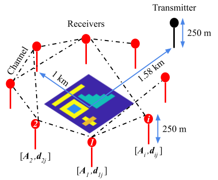
(a)

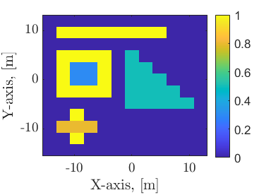
(b)

Figure 1: Illustration of multistatic radar interferometric imaging scene (a). In the distributed network each agent $i$ can access a subset of the data (i.e. $[\boldsymbol{A}_{i},\boldsymbol{d}_{ij}]$). Scene reflectivity function used in numerical simulations (b), $12\times 12$ image with a pixel spacing of 2.4 m.

Many algorithms used to solve the centralized interferometric imaging problem take inspiration from phase retrieval problems (Candés et al., 2013, 2015; Duchi and Ruan, 2018). A gradient-descent-based iterative low rank matrix recovery approach was proposed in Mason et al. (2015); which lifts the solution set to convexify the problem, leading to increased complexity. Recently, Yonel and Yazici (2019) and Yonel et al. (2020) proposed a generalized Wirtinger flow (GWF) algorithm to solve the interferometric problem, which operates in the signal domain resulting in improved computation and memory efficiencies. They show that the GWF algorithm can achieve a linear convergence rate under specific conditions on the measurements (Yonel and Yazici, 2019). Demanet and Jugnon (2017) solve the centralized interferometric imaging problem using a lifting approach with a graph to encode the available interferometric measurements. They establish a relationship between graph connectivity and the robustness of recovery.

Recently, distributed optimization techniques have been proposed to solve the phase retrieval problem. Zhao et al. (2018) introduced the distributed Wirtinger flow algorithm (DWF) to solve the phase retrieval problem using a perturbed proximal primal-dual approach. The authors in Zhao et al. (2018) show that DWF can converge to an approximate solution at a sublinear rate. Chen et al. (2020) introduced a distributed subgradient method to solve weakly convex and non-smooth problems such as the phase retrieval problem. They report a linear convergence rate, using the gradient norm as a stopping criterion when the function is locally sharp near a minimizer.

In this work, to the best of our knowledge (Demanet and Jugnon, 2017; Yonel and Yazici, 2019; Yonel et al., 2020), we present the first distributed nonconvex primal-dual optimization algorithm to solve the interferometric imaging problem. The contributions of this paper are:

• We show that the Polyak-Łojasiewicz (PL) inequality is satisfied for the interferometric imaging problem when its lifted forward model meets the restricted isometry properties of rank-1 positive semi-definite matrices with a sufficiently small restricted isometry constant.

• We show that after proper initialization the Distributed Generalized Wirtinger Flow (DGWF) algorithm converges linearly to a global optimum when the cost function is smooth and PL inequality is satisfied.

• We provide numerical evidence that the DGWF algorithm can achieve comparable image reconstruction quality to centralized methods (Yonel and Yazici, 2019; Yonel et al., 2020) for radar interferometric imaging applications.

This paper is organized as follows. Section 2 provides the problem formulation. Section 3 introduces the proposed DGWF algorithm. Section 4 shows linear convergence for the DGWF algorithm. Numerical simulations are in Section 5, and Section 6 concludes this paper.

2 Problem Formulation

Suppose the desired signal is denoted by $x\in\mathbb{C}^{K}$, the interferometric imaging problem can be formulated as:

$$\textrm{find}\quad\quad x$$

$$\textrm{subject to}\quad d_{ij}^{s}=\langle a_{i}^{s},x\rangle\overline{\langle a_{j}^{s},x\rangle},$$

$$\textrm{for}\quad i=1,2,...,N;j\neq i;s=1,2,...,S$$

where $d_{ij}^{s}\in\mathbb{C}$ is the $s^{th}$ cross-correlation sample for the $i^{th}$ and $j^{th}$ sensing processes, $a_{i}^{s}\in\mathbb{C}^{K}$ is the $s^{th}$ sampling vector for the $i^{th}$ sensing process, $\overline{(\cdot)}$ is the complex conjugate, and $\langle.,.\rangle$ denotes the inner product.

Now, consider a connected network with $N$ agents defined by the undirected graph $\mathcal{G}=\{\mathcal{V},\mathcal{E}\}$ with $|\mathcal{V}|=N$ vertices and $|\mathcal{E}|=E$ edges. We assume the graph $\mathcal{G}$ does not contain self-loops and let $L$ denote the graph’s Laplacian matrix. Agents try to cooperatively solve the following optimization problem,

$$\min_{x\in\mathbb{C}^{K}}f(x):=\frac{1}{N}\sum_{i=1}^{N}f_{i}(x).$$ (1)

Let $\mathcal{X}^{*}$ and $f^{*}$ denote the optimal set and the minimum function value for optimization Problem (1). In practice the cross-correlation measurements $d_{ij}^{s}$ are assumed to be corrupted with additive i.i.d. noise. To recover $x$, each agent $i$ formulates a local least squares error minimization objective function defined as,

$$f_{i}(x)=\frac{1}{2|\mathcal{N}_{i}|S_{i}}\sum_{j\in\mathcal{N}_{i}}\sum_{s=1}^{S_{i}}|d_{ij}^{s}-\langle a_{i}^{s},x\rangle\overline{\langle a_{j}^{s},x\rangle}|^{2},$$ (2)

which can be thought of as the sensing process associated with the $i^{th}$ agent of the network (Yonel and Yazici, 2019). Agent $i$’s neighbors are defined as $\mathcal{N}_{i}\triangleq\{i\in\mathcal{V}|j\in\mathcal{V},(i,j)\in\mathcal{E}\}$. The term $S_{i}$ denotes the number of cross-correlation samples agent $i$ measures. Thus the graph influences the optimization process and the number of cross-correlation measurements that can be computed.

Next we state two technical assumptions that will help us later prove convergence for the DGWF algorithm.

Assumption 1

The undirected graph $\mathcal{G}$ is connected.

Assumption 2

The optimal set $\mathcal{X}^{*}$ of (1) is nonempty and $f^{*}>-\infty$.

Exploiting the structure of the graph Laplacian $L$, we can thus write the distributed interferometric imaging Problem (1) equivalently as,

$$\min_{\boldsymbol{x}\in\mathbb{C}^{NK}}\tilde{f}(\boldsymbol{x})$$ (3)

$$\textrm{s.t. }\boldsymbol{L}\boldsymbol{x}=\boldsymbol{0}_{NK},$$

where $\boldsymbol{x}=\textrm{col}(x_{1},...,x_{N})$, $\tilde{f}(\boldsymbol{x})=\sum_{i=1}^{N}f_{i}(x_{i})$, and $\boldsymbol{L}=L\otimes I_{K}$ where $L$ is the graph Laplacian and $\otimes$ is the Kronecker product (Uribe et al., 2021).

3 Distributed Generalized Wirtinger Flow Algorithm

Recently, Yi et al. (2021) presented an algorithm for distributed nonconvex optimization that converges linearly if the local and global cost function is smooth and satisfies the PL inequality, respectively. We propose a primal-dual algorithm inspired by Yi et al. (2021) that uses Wirtinger derivatives  (Yonel and Yazici, 2019). We call the proposed algorithm the Distributed Generalized Wirtinger Flow (DGWF) algorithm.

Following the algorithm formulation presented in Yi et al. (2021), the augmented Lagrangian function for (3) can be written as,

$$\mathcal{A}(\boldsymbol{x},\boldsymbol{u})=\tilde{f}(\boldsymbol{x})+\frac{\lambda_{1}}{2}\boldsymbol{x}^{\top}\boldsymbol{L}\boldsymbol{x}+\lambda_{2}\boldsymbol{u}^{\top}\boldsymbol{L}^{1/2}\boldsymbol{x},$$ (4)

where $\lambda_{1}>0$ and $\lambda_{2}>0$ are the regularization parameters, $\boldsymbol{u}\in\mathbb{C}^{NK}$ is the dual variable, and the constraint $\boldsymbol{L}\boldsymbol{x}=\boldsymbol{0}_{NK}$ is replaced with its equivalent $\boldsymbol{L}^{1/2}\boldsymbol{x}=\boldsymbol{0}_{NK}$ since its nulls are identical (Uribe et al., 2021). Yi et al. (2021) proposed the following first order primal-dual gradient method to solve (4),

$$\boldsymbol{x}_{t+1} =\boldsymbol{x}_{t}-\frac{\eta}{\|x_{0}\|}(\lambda_{1}\boldsymbol{L}\boldsymbol{x}_{t}+\lambda_{2}\boldsymbol{L}^{1/2}\boldsymbol{u}_{t}+\nabla\tilde{f}(\boldsymbol{x}_{t}))$$ (5)

$$\boldsymbol{u}_{t+1} =\boldsymbol{u}_{t}+\frac{\eta}{\|x_{0}\|}\lambda_{2}\boldsymbol{L}^{1/2}\boldsymbol{x}_{t},\quad\forall\boldsymbol{x}_{t}\in\mathbb{C}^{NK},$$ (6)

where $\eta>0$ is the step size and $\|x_{0}\|$ is the norm of the initial estimate. If we denote $\boldsymbol{v}_{t}=\boldsymbol{L}^{1/2}\boldsymbol{u}_{t}$, we can rewrite (5) and (6) as,

$$\boldsymbol{x}_{t+1} =\boldsymbol{x}_{t}-\frac{\eta}{\|x_{0}\|}(\lambda_{1}\boldsymbol{L}\boldsymbol{x}_{t}+\lambda_{2}\boldsymbol{v}_{t}+\nabla\tilde{f}(\boldsymbol{x}_{t}))$$ (7)

$$\boldsymbol{v}_{t+1} =\boldsymbol{v}_{t}{+}\frac{\eta}{\|x_{0}\|}\lambda_{2}\boldsymbol{L}\boldsymbol{x}_{t},\forall\boldsymbol{x}_{t}\in\mathbb{C}^{NK},\sum_{j=1}^{N}v_{j,0}=\boldsymbol{0}_{K}.$$ (8)

For initializing the DGWF algorithm we adopt the spectral initialization scheme used in Yonel and Yazici (2019); Yonel et al. (2020). The initial estimate $x_{0}\in\mathbb{C}^{K}$ is the rank-1, positive semi-definite matrix approximation of the lifted backprojection estimate $\hat{\boldsymbol{X}}\in\mathbb{C}^{K\times K}$,

$$\hat{\boldsymbol{X}}{:=}\frac{1}{N}\sum_{i=1}^{N}\frac{1}{2|\mathcal{N}_{i}|S_{i}}\sum_{j\in\mathcal{N}_{i}}\sum_{s=1}^{S_{i}}d_{ij}^{s}a_{i}^{s}(a_{j}^{s})^{H}{+}\overline{d_{ij}^{s}}a_{j}^{s}(a_{i}^{s})^{H},$$ (9)

where $x_{0}=\sqrt{\lambda_{0}}\mathbf{v}_{0}$ with $\lambda_{0},\mathbf{v}_{0}$ being the leading eigenvalue-eigenvector pair of $\hat{\boldsymbol{X}}$ and $(\cdot)^{H}$ denotes the complex conjugate transpose. The lifted formulation of the $i^{th}$ and $j^{th}$ sensing processes is $F^{s}=a_{j}^{s}(a_{i}^{s})^{H}$. Let $\boldsymbol{d}=[d_{ij}^{1},d_{ij}^{2},...,d_{ij}^{S}]\in\mathbb{C}^{S}$ denote the vector of cross-correlated measurements. The lifted forward model $\mathcal{F}:\mathbb{C}^{K\times K}\rightarrow\mathbb{C}^{S}$ is defined as,

$$\boldsymbol{d}=\mathcal{F}(\hat{\boldsymbol{X}}),$$ (10)

where $\mathcal{F}$ is a $[S\times K^{2}]$ matrix with $F^{s}$ as its rows and $\hat{\boldsymbol{X}}$ concatenated into a vector. This spectral method initializes the iterates within a bounded set i.e., $\mathcal{X}=\{x\,|\,\|x\|^{2}\leq\tau\}$, where $\tau$ is a constant dependent on the restricted isometry constant over rank-1 matrices (RIC${}_{\delta_{1}}$) for the lifted forward model (10) (Yonel and Yazici, 2019, Theorem 4.6). The initial estimate is distributed to all agents, i.e., $x_{0}=x_{1,0}=x_{2,0}=...=x_{i,0}$.

Remark 3

The spectral initialization (9) computes a rank-1 approximation to a low rank matrix recovery problem using all the local cross-correlation measurements stored at every agent. The lifted backprojection estimate $\hat{\boldsymbol{X}}$ is an average over all local lifted backprojection estimates. Thus, one possible way to create a distributed initialization method would be to run a distributed averaging algorithm over the local lifted backprojection estimates (Olshevsky and Tsitsiklis, 2009). Analysis of how distributed initialization schemes effect the DGWF algorithm is left for future work.

The DGWF algorithm using spectral initialization (9) and updates (7), (8) is shown in pseudo-code as Algorithm 1.

Algorithm 1 Distributed Generalized Wirtinger Flow

0:  parameters $\lambda_{1}>0,\lambda_{2}>0$, and $\eta>0$

0:  $x_{i,0}\in\mathbb{C}^{K}$ with (9) and $v_{i,0}=\boldsymbol{0}_{K},\forall i\in[N]$.

1:  for $t=0,1,...$ do

2:     for $i=1,...,N$ in parallel do

3:        Send $x_{i,t}$ to $\mathcal{N}_{i}$ and receive $x_{j,t}$ from $j\in\mathcal{N}_{i}$; Primal variable update:

4:        $x_{i,t+1}=x_{i,t}-\frac{\eta}{\|x_{i,0}\|}(\lambda_{1}\sum_{j\in\mathcal{N}_{i}}L_{ij}x_{j,t}+\lambda_{2}v_{i,t}+\nabla f_{i}(x_{i,t}))$; Dual variable update:

5:        $v_{i,t+1}=v_{i,t}+\frac{\eta}{\|x_{i,0}\|}\lambda_{2}\sum_{j\in\mathcal{N}_{i}}L_{ij}x_{j,t}$;

6:     end for

7:  end for

8:  return  $\boldsymbol{x}_{t}$

The gradient $\nabla f_{i}(x_{i,t})$ is explicitly found by computing the Wirtinger derivative using the local information agent $i$ can access (Yonel and Yazici, 2019). For the cross-correlation between agent $i$ and agent $j$ with $(i,j)\in\mathcal{E}$ the gradient is

$$\nabla f_{i}(x_{i,t}){=}\nabla{\left[\frac{1}{2|\mathcal{N}_{i}|S_{i}}\sum_{j\in\mathcal{N}_{i}}\sum_{s=1}^{S_{i}}|d_{ij}^{s}{-}\langle a_{i}^{s},x_{i,t}\rangle\overline{\langle a_{j}^{s},x_{i,t}\rangle}|^{2}\right]}$$

$${=}\frac{1}{2|\mathcal{N}_{i}|S_{i}}\sum_{j\in\mathcal{N}_{i}}\sum_{s=1}^{S_{i}}\overline{e_{ij}^{s}}\left(a_{j}^{s}(a_{i}^{s})^{H}x_{i,t}\right){+}e_{ij}^{s}\left(a_{i}^{s}(a_{j}^{s})^{H}x_{i,t}\right)$$ (11)

where $e_{ij}^{s}=\left((a_{i}^{s})^{H}x_{i,t}(x_{i,t})^{H}a_{j}^{s}-d_{ij}^{s}\right)$.

In the next section, we show that when the cost function is smooth and satisfies the PL inequality, the DGWF algorithm converges linearly to a minimum.

4 Convergence Analysis

We follow Yonel and Yazici (2019) geometric analysis of the interferometric imaging problem to show when the lifted forward model’s restricted isometry properties over rank-1 positive semi-definite matrices satisfy the Regularity Condition (RC). Then we extend our analysis to show that the RC implies the PL inequality. Finally, convergence of the DGWF algorithm is established.

The RC bounds the local smoothness and curvature of a function, meaning that the function’s gradients are well behaved.

Definition 4

(Regularity Condition): A function $f$ satisfies the RC($\alpha$,$\beta$) with $\alpha,\beta>0$ if,

$$\langle\nabla f(z),z-x^{*}\rangle\geq\frac{1}{\alpha}||\nabla f(z)||^{2}+\frac{1}{\beta}||z-x^{*}||^{2},$$ (12)

for all $z\in\mathbb{R}^{2K}$ and $x^{*}$ being a minimizer of $f$.

Next, the PL inequality is defined. The PL inequality does not require convexity but implies that every stationary point is a global minimizer.

Definition 5

(Polyak-Łojasiewicz Inequality): The function $f$ satisfies the PL inequality if, for some $\mu>0$,

$$\frac{1}{2}||\nabla f(z)||^{2}\geq\mu(f(z)-f^{*}),\quad\forall z\in\mathbb{R}^{2K},$$ (13)

where $f:\mathbb{R}^{2K}\rightarrow\mathbb{R}$ is continuously differentiable and $f^{*}=\min_{z\in\mathbb{R}^{2K}}f(z)$. When this condition holds the function is $\mu$-PL.

We begin by establishing the relationship between the lifted forward model and the RC using the restricted isometry property (RIP). The RIP arose from the compressed sensing field as a way to measure how close a matrix is to an orthonormal system given a certain degree of sparsity (Candes and Tao, 2005).

Definition 6

(Restricted isometry property): Let $\mathcal{A}:\mathbb{C}^{M\times K}\rightarrow\mathbb{C}^{S}$ denote a linear operator. Without loss of generality assume $M\leq K$. For every $1\leq r\leq M$, the $r$-restricted isometry constant (RIC) is defined as the smallest $\delta_{r}<1$ such that

$$(1-\delta_{r})\|X\|_{F}^{2}\leq\|\mathcal{A}(X)\|^{2}\leq(1+\delta_{r})\|X\|_{F}^{2}$$ (14)

holds for all matrices $X$ of rank at most $r$, where $\|X\|_{F}=\sqrt{Tr(X^{H}X)}$ denotes the Forbenius norm.

From (Yonel and Yazici, 2019, Theorem 4.6), when the lifted forward model $\mathcal{F}$ satisfies the RIP condition over rank-1 positive semi-definite matrices with a RIC${}_{\delta_{1}}<0.214$ then Definition (4) surely holds with any $\alpha,\beta$ satisfying,

$$\frac{1}{\alpha\|x^{*}\|^{2}}+\frac{c^{2}(\delta_{1})\|x^{*}\|^{2}}{\beta}\leq h(\delta_{1}):=(1-\delta_{2})(1-\epsilon)(2-\epsilon),$$ (15)

where $\epsilon^{2}=(2+\delta_{1})(1-\sqrt{1-\frac{\delta_{1}}{1+\delta_{1}}})+\frac{\delta_{1}^{2}}{8}$, $\delta_{2}=\frac{\sqrt{2}(2+\epsilon)\delta_{1}}{\sqrt{(1-\epsilon)(2-\epsilon)}}$, and $c(\delta_{1})=(2+\epsilon)(1+\epsilon)(1+\delta_{1})$.

4.1 RC & PL Inequality

In this subsection we restate (Yazdani and Hale, 2021, Lemma 1) in Lemma 7 which shows that the RC implies the PL inequality.

Lemma 7 (Yazdani and Hale (2021), Lemma 1)

Let $f$
have a Lipschitz continuous gradient with Lipschitz constant $L_{f}$ and the set $\mathcal{X}^{*}=\{x^{*}\in\mathbb{R}^{2K}|\nabla f(x^{*})=0\}$ is nonempty and finite. If $f$ is RC($\alpha$,$\beta$), then $f$ is ${1}/{(\beta^{2}L_{f})}$-PL.

4.2 DGWF Algorithm Convergence Analysis

Problem (2) is not complex differentiable due to the mapping from $\mathbb{C}^{K}$ to $\mathbb{R}$ (Kreutz-Delgado, 2009). In the DGWF algorithm Wirtinger derivatives are used because they provide an elegant way to compute partial derivatives that are differentiable in the complex domain. However, for the convergence analysis it is more convenient to work in the real-valued domain. Thus we equivalently reformulate (2) to the real-valued domain where it is differentiable (Kreutz-Delgado, 2009). Without loss of generality, we use (2) for the $i^{th}$ and $j^{th}$ sensing processes and define $\tilde{x}\triangleq[\textrm{Re}(x);\textrm{Im}(x)]\in\mathbb{R}^{2K}$, $d_{R}^{s}=\textrm{Re}(d_{ij}^{s})\in\mathbb{R}$, $d_{I}^{s}=\textrm{Im}(d_{ij}^{s})\in\mathbb{R}$, and

$$\tilde{A}_{R}^{s}\triangleq\begin{bmatrix}\tilde{A}_{1}^{s}&\tilde{A}_{2}^{s}\\ -\tilde{A}_{2}^{s}&\tilde{A}_{1}^{s}\end{bmatrix}\in\mathbb{R}^{2K\times 2K},\tilde{A}_{I}^{s}\triangleq\begin{bmatrix}\tilde{A}_{2}^{s}&-\tilde{A}_{1}^{s}\\ \tilde{A}_{1}^{s}&\tilde{A}_{2}^{s}\end{bmatrix}\in\mathbb{R}^{2K\times 2K},$$

with $\tilde{A}_{1}^{s}=\textrm{Re}(a_{i}^{s})^{\top}\textrm{Re}(a_{j}^{s})+\textrm{Im}(a_{i}^{s})^{\top}\textrm{Im}(a_{j}^{s})$, and $\tilde{A}_{2}^{s}=-\textrm{Re}(a_{i}^{s})^{\top}\textrm{Im}(a_{j}^{s})+\textrm{Im}(a_{i}^{s})^{\top}\textrm{Re}(a_{j}^{s})$, for $s=1,2,...,S$. We can equivalently rewrite (2) in terms of $\tilde{x}$ as

$$f(\tilde{x})\triangleq\frac{1}{2S}\sum_{s=1}^{S}\big{(}\big{(}d_{R}^{s}{-}\tilde{x}^{\top}\tilde{A}_{R}^{s}\tilde{x}\big{)}^{2}{+}\big{(}d_{I}^{s}{-}\tilde{x}^{\top}\tilde{A}_{I}^{s}\tilde{x}\big{)}^{2}\big{)}.$$ (16)

Lemma 8

Function $f(\tilde{x})$ has Lipschitz gradient on the set $\tilde{\mathcal{X}}\triangleq\{\tilde{x}\,|\,\|\tilde{x}\|^{2}\leq\tau\}$ with Lipschitz constant given by

$$L_{f}\triangleq \frac{1}{S}\sum_{s=1}^{S}\left(d_{R}^{s}\sigma_{\max}(\tilde{A}_{R}^{s})+d_{I}^{s}\sigma_{\max}(\tilde{A}_{I}^{s})\right.$$

$$\left.+3\tau\left(\sigma_{\max}^{2}(\tilde{A}_{R}^{s})+\sigma_{\max}^{2}(\tilde{A}_{I}^{s})\right)\right).$$ (17)

Using the definition of the Lipschitz continuity, for $\forall u,v\in\tilde{\mathcal{X}}$ we have

$$\left\|\nabla f(u)-\nabla f(v)\right\|$$

$$\leq\frac{1}{S}\Bigg{\|}\sum_{s=1}^{S}\left((d_{R}^{s}-u^{\top}\tilde{A}_{R}^{s}u)\tilde{A}_{R}^{s}u-(d_{R}^{s}-v^{\top}\tilde{A}_{R}^{s}v)\tilde{A}_{R}^{s}v\right.$$

$$\left.\quad+(d_{I}^{s}-u^{\top}\tilde{A}_{I}^{s}u)\tilde{A}_{I}^{s}u-(d_{I}^{s}-v^{\top}\tilde{A}_{I}^{s}v)\tilde{A}_{I}^{s}v\right)\Bigg{\|}$$

$$\leq\frac{1}{S}\sum_{s=1}^{S}\left(d_{R}^{s}\sigma_{\max}(\tilde{A}_{R}^{s})+\|u\|^{2}\sigma_{\max}^{2}(\tilde{A}_{R}^{s})\right)\|u-v\|$$

$$\quad+\frac{1}{S}\sum_{s=1}^{S}\left\|u^{\top}\tilde{A}_{R}^{s}u\tilde{A}_{R}^{s}v-u^{\top}\tilde{A}_{R}^{s}v\tilde{A}_{R}^{s}v\right\|$$

$$\quad+\frac{1}{S}\sum_{s=1}^{S}\left\|u^{\top}\tilde{A}_{R}^{s}v\tilde{A}_{R}^{s}v-v^{\top}\tilde{A}_{R}^{s}v\tilde{A}_{R}^{s}v\right\|$$

$$\quad+\frac{1}{S}\sum_{s=1}^{S}\left(d_{I}^{s}\sigma_{\max}(\tilde{A}_{I}^{s})+\|u\|^{2}\sigma_{\max}^{2}(\tilde{A}_{I}^{s})\right)\|u-v\|$$

$$\quad+\frac{1}{S}\sum_{s=1}^{S}\left\|u^{\top}\tilde{A}_{I}^{s}u\tilde{A}_{I}^{s}v-u^{\top}\tilde{A}_{I}^{s}v\tilde{A}_{I}^{s}v\right\|$$

$$\quad+\frac{1}{S}\sum_{s=1}^{S}\left\|u^{\top}\tilde{A}_{I}^{s}v\tilde{A}_{I}^{s}v-v^{\top}\tilde{A}_{I}^{s}v\tilde{A}_{I}^{s}v\right\|$$

$$\leq\frac{1}{S}\sum_{s=1}^{S}\left(d_{R}^{s}\sigma_{\max}(\tilde{A_{R}^{s}})+d_{I}^{s}\sigma_{\max}(\tilde{A}_{I}^{s})\right.$$

$$\quad\left.+3\tau\left(\sigma_{\max}^{2}(\tilde{A}_{R}^{s})+\sigma_{\max}^{2}(\tilde{A}_{I}^{s})\right)\right)\|u-v\|.$$

Proposition 9

Let the lifted forward model (10) satisfy the RIP condition over rank-1 positive semi-definite matrices with a RIC${}_{\delta_{1}}\leq 0.214$ (Yonel and Yazici, 2019, Theorem 4.6) and Assumptions 1-2 hold. Moreover, let $\{\tilde{\boldsymbol{x}}_{k}\}$ be the sequence generated by Algorithm 1 with $\lambda_{1}>0$, $\lambda_{2}>0$, $\eta>0$ applied to (16). Then, there exists a $c_{1}>0$, and $\kappa\in(0,1)$ such that,

$$\|\tilde{\boldsymbol{x}}_{t}-\bar{\tilde{\boldsymbol{x}}}_{t}\|^{2}+N(f(\bar{\tilde{x}}_{t})-f^{*})\leq(1-\kappa)^{t}c_{1},\quad\forall t\in\mathbb{N}_{0}.$$ (18)

where $\bar{\tilde{x}}_{t}=\frac{1}{N}(\boldsymbol{1}_{N}^{\top}\otimes\boldsymbol{I}_{K})\boldsymbol{\tilde{x}}_{t}$ and $\bar{\tilde{\boldsymbol{x}}}_{t}=\boldsymbol{1}_{N}\otimes\bar{\tilde{x}}_{t}$.

It follows from Lemma 8 that (16) is smooth with Lipschitz constant (8). Moreover, if the lifted forward model (10) satisfy the RIP condition over rank-1 positive semi-definite matrices with a RIC${}_{\delta_{1}}\leq 0.214$ (Yonel and Yazici, 2019, Theorem 4.6) it holds that (16) is RC, and thus the PL inequality holds from Lemma 7. Finally, the desired result follows from (Yi et al., 2021, Theorem 2).

Remark 10

Due to space limitations the constants $\lambda_{1}$, $\lambda_{2}$, $\eta$, $c_{1}$ and $\kappa$ are not explicitly stated. However they can be directly derived from (Yi et al., 2021, Theorem 1).

5 Numerical Simulations

We consider the system model in Fig. 1, where $N$ independent receivers encircle a region of interest to be imaged with $p_{i}^{rx}\in\mathbb{R}^{3}$ being the spatial position of the $i^{th}$ receiver. A single transmitter of opportunity at a known spatial position $p^{tx}\in\mathbb{R}^{3}$ illuminates the imaging scene. The imaging scene domain $D$ can be discretized into $K$ voxels at positions $x\in\mathbb{R}^{K\times 3}$. The reflectivity function $\rho(x)\in\mathbb{C}^{K}$ for the imaging scene is assumed to be nonfluctuating. Assuming the Born approximation (single bounce) and free-space propagation the frequency domain Green’s function solution to the Helmholtz equation for receiver $i$ can be written as (Yonel and Yazici, 2019),

$$h_{i}(\omega_{s}):=J(\omega_{s})\int_{D}e^{-i\omega_{s}\frac{\phi_{i}(x)}{c_{0}}}\alpha_{i}(x,p^{tx})\rho(x)dx,$$ (19)

where $\omega_{s}$ is the $s^{th}$ discretized temporal frequency of the transmitted signal, $J(\omega_{s})$ is the transmitted signal power, $c_{0}$ is the wave velocity, $\alpha_{i}(x,p^{tx})$ models the propagation attenuation and hardware gains, $\rho(x)$ is the scene reflectivity at position $x\in D$. The $\phi_{i}(x)=|x-p_{i}^{rx}|+|x-p^{tx}|$ is the bi-static delay term due to propagation. The radar interferometric imaging model for the $s^{th}$ temporal frequency sample of the $i^{th}$ and $j^{th}$ receivers in the multistatic radar setup can be formulated as,

$$d_{ij}(\omega_{s})=\sum_{k=1}^{K}\alpha_{i}(x_{k},p^{tx})e^{-i\omega_{s}(|x_{k}-p_{i}^{rx}|+|x_{k}-p^{tx}|)/c_{0}}\rho_{k}\times\\ J(\omega_{s})\overline{J(\omega_{s})}\sum_{k^{\prime}=1}^{K}\overline{\alpha_{j}(x_{k^{\prime}},p^{tx})}e^{i\omega_{s}(|x_{k^{\prime}}-p_{j}^{rx}|+|x_{k^{\prime}}-p^{tx}|)/c_{0}}\overline{\rho_{k^{\prime}}}.$$ (20)

From (20) the linear sampling vectors $a_{i}^{s}$ and $a_{j}^{s}$ can be formulated as,

$$a_{i}^{s} =\left[J(\omega_{s})\alpha_{i}(x_{k},p^{tx})e^{-i\omega_{s}(|x_{k}-p_{i}^{rx}|+|x_{k}-p^{tx}|)/c_{0}}\right]_{k=1}^{K}$$ (21)

$$a_{j}^{s} =\left[J(\omega_{s})\alpha_{j}(x_{k},p^{tx})e^{-i\omega_{s}(|x_{k}-p_{j}^{rx}|+|x_{k}-p^{tx}|)/c_{0}}\right]_{k=1}^{K}.$$ (22)

Combing (20) - (22) the radar interferometric imaging model can be vectorized as,

$$d_{ij}(\omega_{s})=\langle a_{i}^{s},\rho\rangle\overline{\langle a_{j}^{s},\rho\rangle},\quad s=1,...,S;i=1,...,N,j\neq i$$ (23)

The simulated true scene reflectivity function and multistatic radar setup is shown in Fig. 1. Unless otherwise stated the following assumptions and parameters are assumed: Born approximation, $S=64$ frequency samples, $N=35$ receivers, $t_{max}=4000$ for GWF, DGWF max iterations, stepsize $\eta_{t}=\min(1-\exp(-t/\tau_{0}),0.01)$ where $\tau_{0}=3300$, center frequency $12$ GHz, bandwidth $60$ MHz, image is $12\times 12$ $(K=144)$ with spacing $\Delta=2.4$ m since Fourier resolution limit $\Delta_{res}=2.5$ m, graph $\mathcal{G}$ is small-world with a $0.1$ probability of connection, $\lambda_{1}$ and $\lambda_{2}=1$, signal-to-noise ratio is $50$ dB, and transmitter and receiver gains are $100$ dB.

The mean square error (MSE): $\textrm{MSE}\triangleq\frac{1}{K}\sum_{k=1}^{K}(\rho_{i,k}-\rho_{k}^{*})^{2}$ is used to quantitatively determine the accuracy of the reconstructed image $\rho_{i}$ to the true image $\rho^{*}$. For the proposed DGWF algorithm the consensus error $\triangleq\sum_{i=1}^{N}||\rho_{i}-\frac{1}{N}\sum_{i=1}^{N}\rho_{i}||^{2}$. For each simulation the DGWF algorithm is compared to the centralized GWF algorithm (Yonel and Yazici, 2019; Yonel et al., 2020) using the same cross-correlation measurements as defined by the graph.

5.1 Effect of Graph Connectivity

We examine the effects graph connectivity has on the DGWF algorithm’s reconstruction performance. Since the graph specifies how agents communicate and form cross-correlation measurements, we expect the speed of convergence and image reconstruction quality to increase as graph connectivity increases. To test the relationship between graph connectivity and reconstruction performance, we vary the probability of connection for small-world graphs (Watts and Strogatz, 1998) consisting of $35$ agents and record the number of iterations it takes DGWF and GWF to each achieve an MSE of $10^{-5}$. For an additional benchmark, we compare DGWF and GWF against GWF_cg, which is the GWF algorithm using a complete graph. Figure 2(a) shows that decreased graph connectivity results in longer convergence times for GWF and DGWF. However, after the small-world network’s connectivity parameter is greater than $0.4$ there is a negligible change in the number of iterations required to reach the desired reconstruction accuracy.

Additionally, we run the DGWF and GWF algorithms for $10^{5}$ iterations. Figure 2(b) shows that DGWF takes longer to converge compared to GWF because DGWF needs to distribute local information between neighboring agents. The DGWF algorithm reaches a competitive MSE relative to the GWF algorithm without centralized data processing. Figure 2(c) shows that the proposed DGWF algorithm reaches consensus.

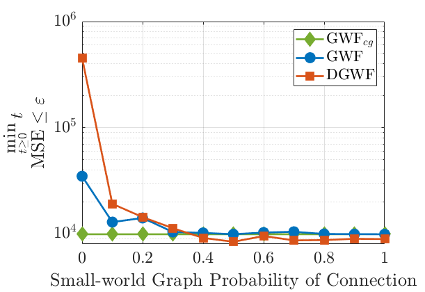
(a)

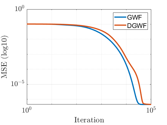
(b)

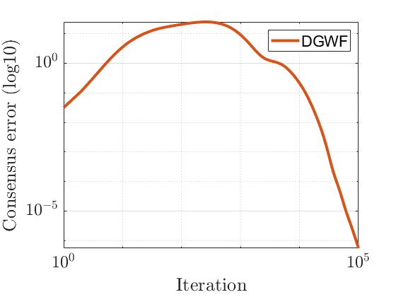
(c)

Figure 2: Comparison between the number of iterations $t$ to reach an MSE $\varepsilon=10^{-5}$ and the connectivity probability of a small-world graph with $35$ agents (2(a)). GWF_cg is GWF using a complete graph. MSE (2(b)) and consensus error (2(c)) per iteration.

5.2 Effect of Number of Receivers

Next, we analyze the effect the number of receivers has on the convergence behavior for the DGWF and GWF algorithms. We vary the number of agents between 5 and 40 and record the MSE for the DGWF and GWF algorithms after $4000$ iterations. Since the number of receivers directly influences the number of cross-correlation measurements each algorithm can compute, we expect that as the number of receivers decreases, the MSE will increase. In Fig. 3(a) the MSE curves for both the DGWF and GWF algorithms show that decreasing the number of receivers increases the reconstruction MSE. Furthermore, Fig. 3(a) suggests that after approximately 30 receivers, the addition of more receivers does not significantly decrease the reconstruction error. Example image reconstructions for the DGWF algorithm for 15 and 40 receivers are presented in Fig. 3(b)-3(c). It can be observed that when the number of receivers is below 30, the DGWF algorithm reconstructs noticeably degraded images. However, when the number of receivers exceeds 30, the DGWF algorithm achieves significantly accurate image reconstructions.

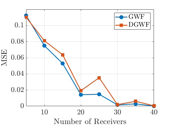
(a)

(b) 15 receivers.

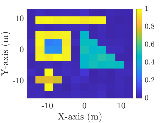
(c) 40 receivers.

Figure 3: Comparison of reconstruction MSE vs. the number of receivers (3(a)). DGWF reconstructions after 4000 iterations for 15 (3(b)) and 40 (3(c)) receivers.

6 Conclusion

We studied the distributed interferometric imaging problem over networks. We combine GWF theory (Yonel and Yazici, 2019) and distributed optimization methods to create the first distributed interferometric imaging algorithm named the Distributed Generalized Wirtinger Flow (DGWF) algorithm. The DGWF algorithm converges linearly to a global optimum with proper initialization and when the cost function is smooth and satisfies the PL inequality. We demonstrate the capabilities of DGWF through numerical radar interferometric imaging simulations. Future work will study convergence analysis for accelerated methods, time-varying directed graphs, and distributed initialization methods.

References

• Candes and Tao (2005) Candes, E. and Tao, T. (2005). Decoding by linear programming. IEEE Transactions on Information Theory, 51(12), 4203–4215.
• Candés et al. (2015) Candés, E.J., Li, X., and Soltanolkotabi, M. (2015). Phase retrieval via wirtinger flow: Theory and algorithms. IEEE Transactions on Information Theory, 61, 1985–2007.
• Candés et al. (2013) Candés, E.J., Strohmer, T., and Voroninski, V. (2013). Phaselift: Exact and stable signal recovery from magnitude measurements via convex programming. Communications on Pure and Applied Mathematics, 66, 1241–1274.
• Chen et al. (2020) Chen, S., García, A., and Shahrampour, S. (2020). Distributed projected subgradient method for weakly convex optimization. ArXiv, abs/2004.13233.
• Demanet and Jugnon (2017) Demanet, L. and Jugnon, V. (2017). Convex recovery from interferometric measurements. IEEE Transactions on Computational Imaging, 3, 282–295.
• Duchi and Ruan (2018) Duchi, J.C. and Ruan, F. (2018). Solving (most) of a set of quadratic equalities: composite optimization for robust phase retrieval. Information and Inference: A Journal of the IMA, 8(3), 471–529.
• Garnier and Papanicolaou (2009) Garnier, J. and Papanicolaou, G. (2009). Passive sensor imaging using cross correlations of noisy signals in a scattering medium. SIAM Journal on Imaging Sciences, 2, 396–437.
• Kreutz-Delgado (2009) Kreutz-Delgado, K. (2009). The complex gradient operator and the cr-calculus.
• Mason et al. (2015) Mason, E., Son, I.Y., and Yazici, B. (2015). Passive synthetic aperture radar imaging using low-rank matrix recovery methods. IEEE Journal of Selected Topics in Signal Processing, 9, 1570–1582.
• Olshevsky and Tsitsiklis (2009) Olshevsky, A. and Tsitsiklis, J.N. (2009). Convergence speed in distributed consensus and averaging. SIAM Journal on Control and Optimization, 48(1), 33–55.
• Uribe et al. (2021) Uribe, C.A., Lee, S., Gasnikov, A., and Nedić, A. (2021). A dual approach for optimal algorithms in distributed optimization over networks. Optimization Methods and Software, 36(1), 171–210.
• Vakalis et al. (2019) Vakalis, S., Gong, L., and Nanzer, J. (2019). Imaging with wifi. IEEE Access, 7, 28616–28624.
• Watts and Strogatz (1998) Watts, D.J. and Strogatz, S.H. (1998). Collective dynamics of ’small-world’ networks. Nature, 393, 440–442.
• Yazdani and Hale (2021) Yazdani, K. and Hale, M. (2021). Asynchronous parallel nonconvex optimization under the polyak łojasiewicz condition. IEEE Control Systems Letters, 6, 524–529.
• Yi et al. (2021) Yi, X., Zhang, S., Yang, T., Chai, T., and Johansson, K.H. (2021). Linear convergence of first- and zeroth-order primal-dual algorithms for distributed nonconvex optimization. IEEE Transactions on Automatic Control, 1–1.
• Yonel et al. (2020) Yonel, B., Son, I.Y., and Yazici, B. (2020). Exact multistatic interferometric imaging via generalized wirtinger flow. IEEE Transactions on Computational Imaging, 6, 711–726.
• Yonel and Yazici (2019) Yonel, B. and Yazici, B. (2019). A generalization of wirtinger flow for exact interferometric inversion. SIAM J. Imaging Sciences, 12, 2119–2164.
• Zhao et al. (2018) Zhao, Z., Lu, S., Hong, M., and Palomar, D.P. (2018). Distributed optimization for generalized phase retrieval over networks. 2018 52nd Asilomar Conference on Signals, Systems, and Computers, 48–52.