Characterizing quantum criticality and steered coherence in the XY-Gamma chain

Abstract

In this paper, we show that an effective spin Hamiltonian with various types of couplings can be engineered using quantum simulators in atomic-molecular-optical laboratories, dubbed the XY-Gamma model. We analytically solve the one-dimensional short-range interacting case with the Jordan-Wigner transformation and establish the phase diagram. In the gapless phase, an incommensurate spiral order is manifested by the vector-chiral correlations. Between distinct gapped phases, a logarithmic scaling behavior of local measures, including spin correlations and the steered quantum coherence, is identified for the quantum critical points, yielding a compelling value of the correlation-length critical exponent. We derive explicit scaling forms of the excitation gap near the quantum critical points. The extracted critical exponents reveal the quantum phase transition on the boundary of Tomonaga-Luttinger liquid belongs to Lifshitz universality class. Our results may provide useful insights into the underlying mechanism in quantum criticality for state-of-the-art experiments of quantum simulation.

I Introduction

The exploration of quantum phenomena is an outstanding challenge and has been one of the most active arenas in condensed matter physics [1]. Novel forms of phases are enriched by ongoing discoveries in transition metal compounds [2, 3, 4, 5], such as spin-orbit-entangled electronic phases [6, 7]. In particular, the quantum spin liquid (QSL) has recently emerged as a new paradigm in correlated electron physics, as it holds promise for the potential application of quantum computing and quantum information. One avenue towards QSL is the focus on highly frustrated materials, exemplified by either the geometrical frustration or the exchange frustration [8, 9, 10, 11]. The triangular, kagome, and pyrochlore structures are categorized into the first type, while the actively sought-after Kitaev magnets belong to the second type. In this context, much attention has been recently devoted towards $4d$ and $5d$ transition metal compounds, due to the interplay between spin-orbit couplings and electronic correlations [12, 13, 14]. The playground to search for the QSL was recently extended to $3d$ transition metal compounds [15]. Despite these endeavors, the Kitaev QSL state has not been conclusively identified among most candidate materials. Certain long-range order (LRO) is unexpectedly found in a variety of Mott insulators, indicating the existence of more conventional types of exchanges beyond a dominant bond-directional Kitaev interaction in these nonideal materials.

Since engineering robust QSL states remains challenging in spin-orbit-entangled candidate materials, an alternative route for exploring novel phases of matter and forms of entanglement is the experimental implementation with the help of other quantum systems in the laboratory. After Feynman’s proposal in 1982 [16], the field of quantum simulation has been developing rapidly for decades and nowadays enables the investigation of quantum systems in a programmable fashion. Especially, recent advances of the laser technology and the laser manipulation of atomic gases have made it feasible to implement a wide class of analog quantum simulations in atomic-molecular-optical (AMO) laboratories. Quantum simulators have been realized on a few platforms, e.g., ultracold atoms [17], polar molecules [18], trapped ions [19, 20], photonic systems [21, 22, 23], and Rydberg atom arrays [24, 25], etc. These systems can be finely tuned in a sufficiently precise way and observed in real time. The effective many-body Hamiltonian can be incorporated from recent developments of simulating quantum magnetism and related quantum dynamics using atoms interacting with the same quantum modes, wherein the quantum channel can be the guided modes in the photonic crystal waveguides [21], the photon of cavity modes [26, 27], and the Rydberg dressing states [28]. With present architectures of quantum simulators, a generic Hamiltonian consisting of flexible coupling graphs can be freely realized, offering the opportunity to implement, simulate, and experimentally test fundamental paradigmatic model Hamiltonians.

This paper is organized as follows. In Sec. II, we discuss the possible engineering of the XY-Gamma model using the AMO system facilitated by coherent photon-mediated Raman transitions. In our scenario, the independent control of XX-, YY-, XY- and YX- terms can be achieved by a double $\Lambda$ scheme in neutral atoms. Section III is devoted to exact solutions of the one-dimensional (1D) short-range interacting Hamiltonian using the Jordan-Wigner transformation. Two-site correlations and dimer correlations are then analyzed. Next, the quantum steered coherence is investigated in Sec. IV. A discussion and summary follow in Sec. V.

II Effective model with Photon-mediated atom-atom Interactions

Recently, using photons to mediate controllable atom-atom interactions has been a well-established paradigm in AMO quantum simulation [28, 29, 30, 27]. The constituents of the engineered quantum spin models are not restricted to only Heisenberg-type interactions [31, 32, 33]. The complex photon-mediated interaction graphs, including both their amplitudes and interaction ranges, can be arbitrarily programed by state-of-the-art techniques involving more laser beams, posing envisioned synthetic quantum matter. For instance, it is well known that the LRO is prohibited by the Mermin-Wagner theorem for short-range interacting models with a continuous symmetry in one spatial dimension [34], while the counterpart on a two-dimensional (2D) bipartite lattice is generally expected to host the long-range Néel order for any spin magnitude $S$, although a rigorous proof of the existence of LRO in a 2D $S=1/2$ Heisenberg model is still lacking [35, 36, 37]. The long-range XY order is induced in an XXZ chain by single-mode-cavity-mediated infinite-range interactions [38]. Instead, QSLs are stabilized in a 2D isotropic Heisenberg model by power-law decaying interactions in multimode cavities [27].

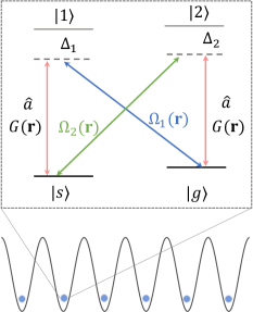
Figure 1: Schematic setups. Atoms are trapped in 1D optical lattice with four-level energy diagram (inset). Two pump lasers with Rabi frequencies $\Omega_{1}$ (blue) and $\Omega_{2}$ (green) induce $\sigma$-transitions between atomic ground and excited states $|g\rangle\leftrightarrow|1\rangle$ and $|s\rangle\leftrightarrow|2\rangle$, respectively. A cavity mode (red) induces $\pi$-transitions between $|s\rangle\leftrightarrow|1\rangle$ and $|g\rangle\leftrightarrow|2\rangle$.

In the following, we consider $N$ atoms that are trapped tightly in a 1D optical lattice, as depicted in Fig. 1. A double $\Lambda$ scheme of an atomic-level diagram is assumed, where two internal atomic states $\{|s\rangle,|g\rangle\}$ in the ground-state manifold represent the pseudospin-$1/2$ states with energy $\{0,\omega_{g}\}$ and two auxiliary excited states $\{|1\rangle,|2\rangle\}$ exist with energy $\{\omega_{1},\omega_{2}\}$, respectively. A photon mode at frequency $\omega_{\mathbf{k}}$ with the field operator $\hat{a}_{\mathbf{k}}$ induces $\pi$-transitions between atomic ground and excited states $|s\rangle\leftrightarrow|1\rangle$ and $|g\rangle\leftrightarrow|2\rangle$, where $\mathbf{k}$ denotes the index of bosonic modes. $G_{\mathbf{k}}(\bf{r})$ is the corresponding spatially dependent coupling strength. Two pump lasers, denoted as $(L1,L2)$ with Rabi strengths $(\Omega_{1},\Omega_{2})$ and frequencies $(\omega_{L1},\omega_{L2})$, are implemented to induce $\sigma$ transitions between atomic ground and excited states, i.e., $|g\rangle\leftrightarrow|1\rangle$ and $|s\rangle\leftrightarrow|2\rangle$, respectively.

Under rotating wave approximation, the atom-light hybrid system is described by the Hamiltonian $\hat{H}=\hat{H}_{0}+\hat{H}_{AL}$, where $\hat{H}_{0}$ is the free Hamiltonian consisting of photon fields $\hat{a}_{\mathbf{k}}$ and atomic Zeeman energy levels $\hat{\sigma}_{j}^{aa}$, and $\hat{H}_{AL}$ is the atom-light interaction Hamiltonian ($\hbar=1$ throughout):

$$\hat{H}_{0} = \sum_{\mathbf{k}}\omega_{\mathbf{k}}\hat{a}^{\dagger}_{\mathbf{k}}\hat{a}_{\mathbf{k}}+\sum_{j}\sum_{\alpha}\omega_{\alpha}\hat{\sigma}^{\alpha\alpha}_{j},$$ (1)

$$\hat{H}_{\rm AL} = \sum_{j}\left[{\Omega_{1}(\mathbf{r}_{j})}e^{-i\omega_{L1}t}\hat{\sigma}_{j}^{1g}+{\Omega_{2}(\mathbf{r}_{j})}e^{-i\omega_{L2}t}\hat{\sigma}_{j}^{2s}+{\rm H.c.}\right]$$ (2)

$$+\sum_{j}\sum_{\mathbf{k}}\left[G_{\mathbf{k}}(\mathbf{r}_{j})\hat{a}_{\mathbf{k}}(\hat{\sigma}_{j}^{1s}+\hat{\sigma}_{j}^{2g})+{\rm H.c.}\right].$$

Here the atomic transition operators are defined as $\hat{\sigma}_{j}^{ab}\equiv|a\rangle_{j}\langle b|$ with four atomic energy levels $a,b=\{g,s,1,2\}$ and $j$ labels the site. Two-atom interaction is synthesized by two Raman transitions, where the photon field $\hat{a}_{\mathbf{k}}$ provides the two-body correlation between the two atoms, as depicted in Fig. 1.

Working in a rotating frame defined by $\hat{U}$=$\exp\{i[\sum_{j}(\omega_{-}\hat{\sigma}_{j}^{gg}+\omega_{+}\hat{\sigma}^{11}_{j}+\omega_{L2}\hat{\sigma}^{22}_{j})+\sum_{\mathbf{k}}\omega_{+}\hat{a}_{\mathbf{k}}^{\dagger}\hat{a}_{\mathbf{k}}]t\}$ with $\omega_{\pm}$=$(\omega_{L2}\pm\omega_{L1})/2$, the transformed Hamiltonian $\tilde{H}=U\hat{H}U^{\dagger}+i(\partial_{t}U)U^{\dagger}$ reads

$$\tilde{H} = -\sum_{\mathbf{k}}\Delta_{\mathbf{k}}\hat{a}^{\dagger}_{\mathbf{k}}\hat{a}_{\mathbf{k}}+\sum_{j}\left[\delta\hat{\sigma}^{gg}_{j}-\Delta_{1}\hat{\sigma}^{11}_{j}-\Delta_{2}\hat{\sigma}^{22}_{j}\right]$$ (3)

$$+\sum_{j}\left[{\Omega_{1}(\mathbf{r}_{j})}\hat{\sigma}_{j}^{1g}+{\Omega_{2}(\mathbf{r}_{j})}\hat{\sigma}_{j}^{2s}+{\rm H.c.}\right]$$

$$+\sum_{j}\sum_{\mathbf{k}}\left[G_{\mathbf{k}}(\mathbf{r}_{j})\hat{a}_{\mathbf{k}}(\hat{\sigma}_{j}^{1s}+\hat{\sigma}_{j}^{2g})+{\rm H.c.}\right],$$

where $\Delta_{\mathbf{k}}\equiv(\omega_{L1}+\omega_{L2})/2-\omega_{\mathbf{k}}$, $\Delta_{1}\equiv(\omega_{L1}+\omega_{L2})/2-\omega_{1}$, $\Delta_{2}\equiv\omega_{L2}-\omega_{2}$ and $\delta=\omega_{g}-(\omega_{L2}-\omega_{L1})/2$. Supposing the frequencies of pump lasers and bosonic modes are all far detuned from the atomic transitions, i.e., $\Delta_{1}$ and $\Delta_{2}$ are much larger than the Rabi coupling coefficients $|\Omega_{1}|,|\Omega_{2}|$, and $|G_{\mathbf{k}}|$, we can safely eliminate the excited states $|1\rangle$ and $|2\rangle$ to obtain the effective Hamiltonian in the ground-state manifold (see Appendix A),

$$\hat{H}_{gs} = \sum_{j}\left[(\delta+V_{g}(\mathbf{r}_{j}))\hat{\sigma}_{j}^{gg}+V_{s}(\mathbf{r}_{j})\hat{\sigma}_{j}^{ss}\right]$$ (4)

$$+\sum_{j}\left[\hat{\sigma}_{j}^{gs}\hat{\Omega}(\mathbf{r}_{j})+\hat{\Omega}^{\dagger}(\mathbf{r}_{j})\hat{\sigma}_{j}^{sg}\right],$$

where $\hat{\Omega}(\mathbf{r})=\Omega_{1}^{\ast}\sum_{\mathbf{k}}G_{\mathbf{k}}(\mathbf{r})\hat{a}_{\mathbf{k}}/\Delta_{1}+\sum_{\mathbf{k}}G^{\ast}_{\mathbf{k}}(\mathbf{r})\hat{a}^{\dagger}_{\mathbf{k}}/\Omega_{2}$ and the light shifts for ground states $V_{g}(\mathbf{r})={|\Omega_{1}|^{2}}/{\Delta_{1}}+{\sum_{kk^{\prime}}G^{\ast}_{\mathbf{k}}G_{\mathbf{k}^{\prime}}\hat{a}^{\dagger}_{\mathbf{k}}\hat{a}_{\mathbf{k}^{\prime}}}/{\Delta_{2}}$, $V_{s}(\mathbf{r})={|\Omega_{2}|^{2}}/{\Delta_{2}}+{\sum_{kk^{\prime}}G^{\ast}_{\mathbf{k}}G_{\mathbf{k}^{\prime}}\hat{a}^{\dagger}_{\mathbf{k}}\hat{a}_{\mathbf{k}^{\prime}}}/{\Delta_{2}}$. In the adiabatic limit due to large detuing or large dissipation $\kappa$ of modes $\hat{a}_{\mathbf{k}}$, the photon field can be approximated by its steady-state value,

$$\hat{a}_{\mathbf{k}}^{\rm ss}=\sum_{j}\,G^{\ast}_{\mathbf{k}}(\mathbf{r}_{j})\left(\frac{\Omega_{1}}{\Delta_{1}}\hat{\sigma}^{-}_{j}+\frac{\Omega_{2}}{\Delta_{2}}\hat{\sigma}^{+}_{j}\right)/{\tilde{\Delta}_{\mathbf{k}}},$$ (5)

with $\tilde{\Delta}_{\mathbf{k}}=\Delta_{\mathbf{k}}+i\kappa-\sum_{j}\,|G_{\mathbf{k}}(\mathbf{r}_{j})|^{2}\left(\hat{\sigma}_{j}^{ss}/{\Delta_{1}}+\hat{\sigma}_{j}^{gg}/{\Delta_{2}}\right)$. Note that here we have included the cavity dissipation $\kappa$ phenomenologically. By adiabatically eliminating the photon degree of freedom, in terms of Pauli operators, $\sigma^{x}_{j}=\hat{\sigma}_{j}^{sg}+\hat{\sigma}_{j}^{gs},\sigma_{j}^{y}=i(\hat{\sigma}^{sg}_{j}-\hat{\sigma}^{gs}_{j}),\sigma^{z}_{j}=\hat{\sigma}_{j}^{gg}-\hat{\sigma}_{j}^{ss}$, we obtain the effective spin Hamiltonian in a compact form,

$$\hat{H}_{\rm int}\! = \sum_{ij}\!(J_{ij}^{x}\sigma_{i}^{x}\sigma_{j}^{x}+J_{ij}^{y}\sigma_{i}^{y}\sigma_{j}^{y})\!+\!J_{ij}^{\rm DM}(\sigma_{i}^{x}\sigma_{j}^{y}-\sigma_{i}^{y}\sigma_{j}^{x})$$ (6)

$$+ \sum_{ij}J_{ij}^{\rm SO}\left(\sigma_{i}^{y}\sigma_{j}^{x}+\sigma_{i}^{x}\sigma_{j}^{y}\right)+\sum_{j}h_{j}^{z}{\sigma}_{j}^{z}.$$

Here $h_{j}^{z}=\delta/2+V_{g}(\mathbf{r}_{j})-V_{s}(\mathbf{r}_{j})$, $J_{ij}^{x}=2$(Re${[\Lambda_{0}]}$+Re${[\Lambda_{1}]}$), $J_{ij}^{y}=$2(Re${[\Lambda_{0}]}$$-$Re${[\Lambda_{1}]}$), $J_{ij}^{\rm DM}=$2Im$[\Lambda_{0}]$, and $J_{ij}^{\rm SO}=$-2Im$[\Lambda_{1}]$, where Re (Im) indicates the real (imaginary) part of a complex variable, $\Lambda_{0,1}\equiv\Lambda_{0,1}(\mathbf{r}_{i},\mathbf{r}_{j})$ with $\Lambda_{0}(\mathbf{r},\mathbf{r}^{\prime})=\sum_{\mathbf{k}}[\frac{\Omega_{1}^{\ast}(\mathbf{r})\Omega_{1}(\mathbf{r}^{\prime})}{\Delta_{1}^{2}\tilde{\Delta}_{\mathbf{k}}}G_{\mathbf{k}}(\mathbf{r})G^{\ast}_{\mathbf{k}}(\mathbf{r}^{\prime})+\frac{\Omega_{2}(\mathbf{r})\Omega_{2}^{\ast}(\mathbf{r}^{\prime})}{\Delta^{2}_{2}\tilde{\Delta}^{\ast}_{\mathbf{k}}}G_{\mathbf{k}}^{\ast}(\mathbf{r})G_{\mathbf{k}}(\mathbf{r}^{\prime})]$ and $\Lambda_{1}(\mathbf{r},\mathbf{r}^{\prime})=\sum_{\mathbf{k}}[\frac{\Omega_{1}^{\ast}(\mathbf{r})\Omega_{2}(\mathbf{r}^{\prime})}{\Delta_{1}\Delta_{2}\tilde{\Delta}_{\mathbf{k}}}G_{\mathbf{k}}(\mathbf{r})G^{\ast}_{\mathbf{k}}(\mathbf{r}^{\prime})+\frac{\Omega_{2}(\mathbf{r})\Omega_{1}^{\ast}(\mathbf{r}^{\prime})}{\Delta_{1}\Delta_{2}\tilde{\Delta}^{\ast}_{\mathbf{k}}}G_{\mathbf{k}}^{\ast}(\mathbf{r})G_{\mathbf{k}}(\mathbf{r}^{\prime})]$. The detailed definitions of coefficients in Eq. (6) are derived in Appendix A.

The first bracketed term of Eq. (6) corresponds to the conventional XY-type interactions, and the term in the second brackets denotes the $z$ component of Dzyaloshinskii-Moriya interactions (DMIs). The cross-couplings in the third brackets between $x$ and $y$ spin components are referred to as symmetric off-diagonal $\Gamma$ interactions. Exotic forms like DMIs originated from spin-orbit couplings [39, 40, 41, 42] and were firstly devised to account for the weak ferromagnetism in antiferromagnetic crystals [2, 3, 4, 5], favoring chiral states such as spin spirals and skyrmions [6, 7]. Concurrently, the importance of pervasive off-diagonal $\Gamma$ interactions can be traced back to the study of the Kitaev-Heisenberg model [8, 9, 10, 11]. Further research suggests that the symmetric off-diagonal $\Gamma$ interactions should also be taken into account to explain the possible QSLs observed in experiments [43, 44, 45, 46, 47, 48].

III Exact solution and correlations

Note that the cavity-mediated spin-spin interactions in Eq. (6) have infinite range if only a single cavity mode is involved. The finite-range interactions are achieved by using a multimode cavity. The photon modes can be the guide modes in photonic crystal waveguides with quasimomentum $\mathbf{k}$ [22, 23, 21], or the near-degenerate transverse cavity modes [49, 50]. In particular, the multifrequency driving also enables finite-range interactions between intracavity atoms in a single-mode cavity, which has been recently realized experimentally [51]. Therefore, an effective Hamiltonian with tunable interaction strength and interaction range can be constructed by using multimodes $\{\hat{a}_{\mathbf{k}}\}$. In this case, the interference of cavity modes may render the beyond-nearest-neighbor couplings to be negligibly small.

In the following, we concentrate on the spin models for an ensemble of spin-1/2 interacting particles on a 1D lattice with nearest‐neighbor interactions only. The spin Hamiltonian can be rewritten as

$$\hat{H} = \sum_{j=1}^{N}J\left(\frac{1+\gamma}{2}\sigma_{j}^{x}\sigma_{j+1}^{x}+\frac{1-\gamma}{2}\sigma_{j}^{y}\sigma_{j+1}^{y}\right)$$ (7)

$$+\sum_{j=1}^{N}\left[\Gamma\left(\sigma_{j}^{x}\sigma_{j+1}^{y}+\alpha\sigma_{j}^{y}\sigma_{j+1}^{x}\right)+h\sigma_{j}^{z}\right],$$

where the antiferromagnetic coupling $J\equiv J_{j,j+1}^{x}+J_{j,j+1}^{y}$ between the nearest-neighbor atoms is set up as an energy unit for simplicity unless otherwise stated, i.e., $J=1$, $\gamma\equiv(J_{j,j+1}^{x}-J_{j,j+1}^{y})/J$ serves as the anisotropy parameter, $\Gamma\equiv J_{j,j+1}^{\rm DM}+J_{j,j+1}^{\rm SO}$ characterizes the amplitude of off-diagonal exchange interactions, $\alpha\equiv(J_{j,j+1}^{\rm SO}-J_{j,j+1}^{\rm DM})/\Gamma$ denotes the relative coefficient of off-diagonal exchange couplings, and $h$ represents the strength of the uniform transverse field. The $\Gamma$ term reduces to the DMI for $\alpha=-1$ and the symmetric off-diagonal exchange interaction for $\alpha=1$. In what follows, we impose periodic boundary conditions (PBCs) with $\sigma_{N+1}^{a}\equiv\sigma_{1}^{a}$ ($a=x,y,z$).

The motivations of exploring the quantum criticality in the XY-Gamma model are two fold. On one hand, the low-dimensional quantum magnets have been particularly of concern owing to their evident quantum aspects and substantial corrections to classical counterparts. The quantum criticalities have been explored in a few magnetic materials. The notable examples range from the spin-1/2 Ising ferromagnet LiHoF₄ [52], SrCo₂V₂O₈ [53], Cs₂CoCI₄ [54], and CoNb₂O₆ [55] to BaCo₂V₂O₈ [56] as well as the spin-1 ferromagnetic Heisenberg chain NiNb₂O₆ [57]. To date, quantum phase transitions (QPTs) of analog models have been studied in different contexts, such as the XY model with DMIs [58]. The simultaneous appearance of off-diagonal exchange $\Gamma$ interactions and XY-type interaction in the presence of external fields, especially counteracting the disordered state, is less systematically clear. One the other hand, the merit of Eq. (6) resides in its exact solvability. The analytical results render the possibility to calculate accurately the experimental measurable quantities, in particular various dynamic ones, and thus serve as a benchmark for more sophisticate models. As we shall demonstrate, the extracted critical exponents can be relevant to the experimental measurement of thermodynamic quantities and information measures.

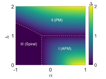
Figure 2: The contour map of excitation gap with respect to $\alpha$ and $h$. The white dashed lines correspond to the critical lines separating phases I (AFM), II (PM), and III (Spiral) of the XY-Gamma model with $J=1.00$, $\Gamma=0.60,\gamma=0.60$.

The Hamiltonian in Eq. (7) is analytically solved by means of Jordan-Wigner, Fourier, and Bogoliubov transformations. The detailed diagonalization procedure is shown in Appendix B.1. Ultimately, the Hamiltonian can be brought into a diagonal form of a less fermion in the momentum space,

$$\hat{H} = \sum_{k}{\varepsilon}_{k}({b}_{k}^{+}{b}_{k}-\frac{1}{2}),$$ (8)

where the energy spectrum of fermionic quasiparticles is

$${\varepsilon}_{k} = 2\sqrt{[\Gamma^{2}(\alpha+1)^{2}+\gamma^{2}]\sin^{2}{k}+(\cos{k}-h)^{2}}$$ (9)

$$-2\Gamma(1-\alpha)\sin{k}.$$

With the excitation energy at hand, the energy gap $\Delta$=$\min_{k}{\varepsilon}_{k}$ can be determined. As shown in Fig. 2, the ground-state phase diagram consists of three phases by varying $\alpha$ and $h$. The horizontal segment $h_{c,1}=1$ for $\alpha>-{\gamma^{2}}/{4\Gamma^{2}}$ separates the gapped phase I and phase II, while the gapless phase III is encompassed by the separatrices $\alpha_{c,1}=-\gamma^{2}/(4\Gamma^{2})$ for $h\leq 1$ and $\alpha_{c,2}=(1-h^{2}-\gamma^{2})/(4\Gamma^{2})$ for $h>1$, or equivalently, $h_{c,2}=\sqrt{1-\gamma^{2}-4\Gamma^{2}\alpha}$ for $\alpha<-\gamma^{2}/(4\Gamma^{2})$.

Typically, one can define spatial and temporal characteristic lengths that have diverging behavior as the control parameter $\lambda$ approaches the threshold value $\lambda_{c}$. This diverging property of characteristic lengths with the correlation-length critical exponent $\nu$ and the dynamical critical exponent $z$ enables one to define universality classes. The critical behavior is determined by those low-energy states near the critical mode. The dynamical exponent $z$ relates the scaling of energy to length scales, which can be retrieved by the shape of the spectra near the gap closing mode $\Delta\sim(k-k_{c})^{z}$. As $\lambda$ approaches $\lambda_{c}$, the gap vanishes as $\Delta\sim(\lambda-\lambda_{c})^{\nu z}$. To this end, we expand Eq. (9) at the critical line $h_{c,1}$ around the gap closing momentum $k_{c}=0$,

$${\varepsilon}_{k}\simeq 2\sqrt{\gamma^{2}+\Gamma^{2}(1+\alpha)^{2}}|k|-2\Gamma(1-\alpha)k.$$ (10)

The relativistic spectra at the critical line $h_{c,1}$ imply that $z$ = 1. The gap near $h_{c,1}$ is approximated as

$$\Delta\simeq\,2|h-h_{c,1}|,$$ (11)

and one then finds $\nu z=1$. In this case, the quantum critical point (QCP) between phase I and phase II belongs to 2D Ising universality class characterized by $\nu=1$, $z=1$. On the verge between gapped phase II and gapless phase III, one can find the spectra vanish at an incommensurate momentum $k_{c}=\arccos(h_{c,2}^{-1})$,

$$\varepsilon_{k}\simeq\left[\frac{\Gamma(1-\alpha)\cos^{2}k_{c}}{2\sin k_{c}}+\frac{(h_{c,2}^{-1}-h_{c,2})^{2}}{2\Gamma(1-\alpha)\sin k_{c}}\right](k-k_{c})^{2}.\quad\quad$$ (12)

The above quadratic dispersion indicates the dynamical exponent $z=2$. While expanding the gap around the QCP from the upper threshold one obtains the excitation as

$$\Delta\simeq\frac{2(h_{c,2}-h_{c,2}^{-1})}{\Gamma(1-\alpha)\sin k_{c}}(h-h_{c,2}).$$ (13)

The critical exponents $\nu=1/2$ and $z=2$ annotate that the QPT is in the so-called Lifshitz universality class [59], which corresponds to the universality class of quantum criticality of free fermions. In the case of the I-III transition $\alpha_{c,1}$, the spectra are found to be quadratic in $k$ around the gap closing mode $k_{c}=\arccos h$ as

$$\varepsilon_{k}\simeq\frac{\sqrt{1-h^{2}}}{\Gamma(1-\alpha)}(k-k_{c})^{2},$$ (14)

which yields $z$=2. Similarly, the gap around the critical point $\alpha_{c,1}$ from above obeys a power-law relation as

$$\Delta\simeq\frac{4\Gamma\sin k_{c}}{1-\alpha_{c,1}}(\alpha-\alpha_{c,1}).$$ (15)

The scaling form in Eq. (15) reveals that the transition also belongs to the Lifshitz universality class with $z$ = 2 and $\nu$ = 1/2.

We also calculate the second derivative of the ground-state energy density $e_{0}=-\sum_{k}|{\varepsilon}_{k}|/(2N)$ in Fig. 3, which showcases extreme values around critical points. With increase of the system sizes, the peaks of $-\partial^{2}e_{0}/\partial h^{2}$ for $\alpha=0.50$ become more pronounced. To be concrete, a logarithmic singularity across the QPT between phase I and phase II is identified as

$$\left(-\frac{\partial^{2}{e_{0}}}{\partial{h^{2}}}\right)_{\rm max} = a_{\rm E}\ln N+c_{1}.$$ (16)

Meanwhile, in the vicinity of the critical point in the thermodynamic limit, one finds

$$\left(-\frac{\partial^{2}{e_{0}}}{\partial{h^{2}}}\right) = b_{\rm E}\ln|h-h_{c}|+c_{2}.$$ (17)

The numerical fittings in Fig. 3(a) yield $a_{\rm E}=0.2871\pm 0.0058$, $c_{1}=0.1878$, $b_{\rm E}=-0.2887\pm 0.0009$, and $c_{2}=0.1162$. According to the logarithmic scaling ansatz [60], the ratio $|a_{E}/b_{E}|$ equals the correlation-length exponent $\nu$ $\simeq 1$, confirming that the QPT from phase I to phase II coincides with a second-order transition. The retrieved specific heat exponent $\alpha$ = $2-(d+z)\nu$=0 validates the scaling relation for the logarithmic scaling in $d=1$ dimension. In contrast, one observes in Fig. 3(b) that $-\partial^{2}e_{0}/\partial\alpha^{2}$ exhibits a size-independent discontinuity at the critical points for $h=0.50$ and $h=1.17$, which is a common feature of the transition between the gapless phase and the gapped phase [61].

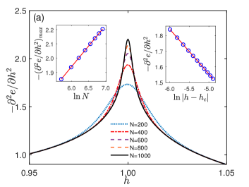
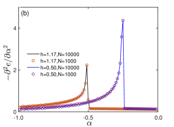
Figure 3: (a) ${-\partial^{2}e/\partial h^{2}}$ as a function of $h$ with $\alpha=0.50$ for various system sizes. The left inset shows the scaling behavior between the maximum value of ${-\partial^{2}e/\partial h^{2}}$ and the system size $N$. The right inset shows $-{\partial^{2}e/\partial h^{2}}$ in the vicinity of the critical point. The symbols denote the numerical results, and the solid lines correspond to the linear fittings. (b) ${-\partial^{2}e/\partial\alpha^{2}}$ vs $\alpha$ with $h=0.50$ and $h=1.17$. Other parameters: $J=1.00$, $\gamma=0.60$, $\Gamma=0.60$.

The nature of the ground state can be gained from the two-qubit correlation functions

$$G_{i,j}^{a,b}=\langle\sigma_{i}^{a}\sigma_{j}^{b}\rangle-\langle\sigma_{i}^{a}\rangle\langle\sigma_{j}^{b}\rangle$$ (18)

with $a$, $b$=$x$, $y$, $z$. In fact, $G_{i,j}^{a,b}$ can be abbreviated as $G_{r}^{a,b}$ with $r=i-j$ due to the translational invariance of Eq. (7). A generic correlation ${\langle{\sigma}_{i}^{a}{\sigma}_{j}^{b}\rangle}$ can be expressed as a Pfaffian form in terms of Wick’s theorem [62], which is the determinant of the $2r\times 2r$ dimensional antisymmetric matrix. The detailed calculation is exhibited in Appendix B.2. One observes that the nearest-neighbor correlation functions display kinks across QCPs between the gapless phase and gapped phases. With increasing $\alpha$ for $h=0.50$ in Fig. 4(a), the dominant nearest-neighbor correlation changes from a positive value of $G_{1}^{yx}$ to a negative value of $G_{1}^{xx}$, implying a QPT from the gapless spiral phase to the gapped antiferromagnetic (AFM) phase. Instead, the ruling correlations $G_{1}^{zz}$ in Fig. 4(b) for $h=1.17$ suggest that phase II belongs to the paramagnetic (PM) phase. Similar trends of correlations for $\alpha=0.50$ are displayed in Fig. 5. The dominating nearest-neighbor correlations change from a negative value of $G_{1}^{xx}$ to a positive value of $G_{1}^{zz}$ across $h_{c,1}$. Therefore, the first-order derivative of $G_{1}^{xx}$ presents a pronounced peak at $h_{c,1}$ in Fig. 5(b). We can further find the first-order derivative of $G_{1}^{xx}$ also follows a logarithmic divergence across the second-order QPT as

$$\left(\frac{\partial G^{xx}}{\partial{h}}\right)_{\rm max}=a_{\rm G}\ln{N}+c_{3},$$ (19)

$$\left(\frac{\partial G^{xx}}{\partial{h}}\right)=b_{\rm G}\ln{|h-h_{c}|}+c_{4},$$ (20)

where $a_{\rm G}=0.2789\pm 0.0045$, $b_{\rm G}=-0.2811\pm 0.0001$, $c_{3}=0.1758,$ and $c_{4}=0.0265$. In this case, one can speculate that $\nu\approx|a_{\rm G}/b_{\rm G}|$=$0.9922\pm 0.0209$, which is quite close to the value retrieved from the second derivative of the ground-state energy density.

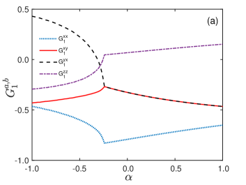
Figure 4: The nearest-neighbor correlation functions with respect to $\alpha$ for (a) $h=0.50$ and (b) $h=1.17$. Other parameters: $N$=2000, $J=1.00$, $\Gamma=0.60$, $\gamma=0.60$.

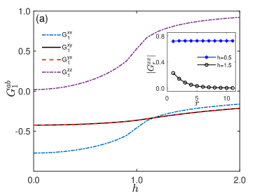
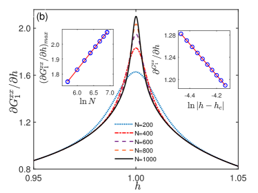
Figure 5: (a) The correlation functions $G_{1}^{xx}$, $G_{1}^{zz}$, $G_{1}^{xy}$, $G_{1}^{yx}$ as a function of $h$ for $\alpha=0.50$. The inset shows $|G_{r}^{zz}|$ vs $r$ for $h=0.50$ and $1.50$ with $N=2000$. (b) The first-order derivative of $G_{1}^{xx}$ with $N=200$, $400$, $600$, $800$, $1000$. The left inset shows the scaling behavior between the maximum value of ${\partial G_{1}^{xx}/\partial h}$ and the system size $N$. The right inset shows $\partial G_{1}^{xx}/\partial h$ in the vicinity of the critical point. The symbols denote the numerical results, and the solid lines correspond to the linear fittings. Other parameters: $J=1.00$, $\gamma=0.60$, $\Gamma=0.60$.

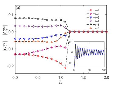
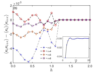
Figure 6: (a) The correlation function $|G_{i,i+r}^{xy}|-|G_{i,i+r}^{yx}|$ with respect to $h$ for different $r$. The inset shows $|G_{i,i+r}^{xy}|-|G_{i,i+r}^{yx}|$ vs $r$ for $h=0.50$. (b) The dimer correlation $\langle\kappa_{i}\kappa_{i+r}\rangle-\langle\kappa_{i}\rangle\langle\kappa_{i+r}\rangle$ with respect to $h$ for different $r$. The inset displays the dimer correlation vs $r$ for $h=0.50$. Other parameters: $N$=2000, $J=1.00$, $\alpha=-0.50$,$\gamma=0.60$, $\Gamma=0.60$.

It is well known that the AFM phase hosts Néel LRO, while the LRO is absent in the PM phase, as is unraveled in the inset of Fig. 5(a). One can further notice that the amplitudes of $G_{1}^{xy}$ and $G_{1}^{yx}$ coincide in the gapped phases, while become unbalanced in the gapless phase. Hence, such a feature suggests that $|G_{1}^{xy}|-|G_{1}^{yx}|$ is a well-defined order parameter to identify the spiral phase for the XY-Gamma model. A natural question arises whether there is LRO in the gapless spiral phase. To probe this question, we numerically calculate the vector-chiral correlations $|G_{r}^{xy}|-|G_{r}^{yx}|$ for different distances $r$ in Fig. 6(a), in which the absolute value is taken in order to remove the indeterminate sign of the numerical Pfaffian calculation. One can find that $|G_{r}^{xy}|-|G_{r}^{yx}|$ is always zero in the gapped phase as a consequence of $G_{r}^{xy}=G_{r}^{yx}$, while it remains finite in the gapless spiral phase. Upon increasing the distance $r$, the correlation presents an oscillating decline as $r^{-1/2}$ shown in Fig. 6(a) [58], suggesting the existence of a quasi-long-range order of an incommensurate spiral order. Next, to delve more deeply into the spiral order, we consider four-qubit correlations as exemplified by the dimer correlation

$$D_{j,j+r}=\langle\kappa_{j}\kappa_{j+r}\rangle-\langle\kappa_{j}\rangle\langle\kappa_{j+r}\rangle,$$ (21)

where the $z$-component vector chiral order parameter is defined by [63, 64]

$$\kappa_{j}=\left(\vec{\sigma}_{j}\times\vec{\sigma}_{j+1}\right)^{z}.$$ (22)

We thus calculate the dimer correlation $D_{j,j+r}$ as a function of $h$ for $\alpha=0.50$ in Fig. 6(b). One observes that the dimer correlations oscillate in the spiral phase and tend to decay with increasing the distance $r$ between the dimers. We further find that dimer correlations persist only for a few sites, and thus the four-qubit correlations decay more rapidly than the two-qubit counterparts.

IV STEERED QUANTUM COHERENCE

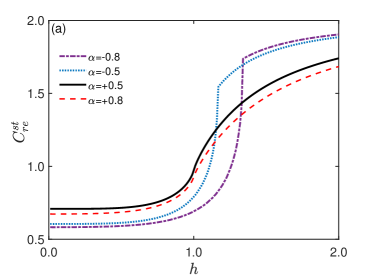
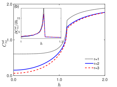
Figure 7: (a) The SQC $C_{re}^{st}$ vs the transverse field $h$. The dash-dotted, dotted, solid and dashed lines correspond to $\alpha=-0.80$, $-0.50$, $0.50$, and $0.80$, respectively.(b) $C_{re}^{st}$ vs $h$ for $\alpha=-0.50$. The dotted, solid and dashed lines correspond to different distances between the two qubits $r=1$, $2$, and $3$. Inset shows the first derivative of $C_{re}^{st}$ with respect to $h$. Other parameters: $N$=2000, $J=1.00$, $\gamma=0.60,\Gamma=0.60$.

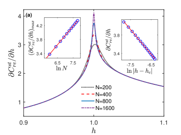
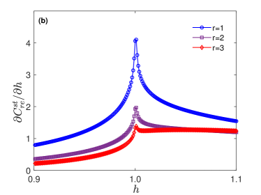
Figure 8: (a)$C_{re}^{st}$ vs $h$ for $\alpha=0.50$. The left inset shows the scaling behavior between the maximum value of ${\partial C_{re}^{st}/\partial h}$ and the system size $N$, and the right inset shows $\partial C_{re}^{st}/\partial h$ in the vicinity of the critical point. (b) The first derivative of $C_{re}^{st}$ with respect to $h$ for $\alpha=0.50$ with $r=1$, $2$, and $r=3$. Other parameters: $N$=2000, $J=1.00$, $\gamma=0.60,\Gamma=0.60$.

In recent years, a few approaches inherited from quantum information have been employed to characterize the QPTs, such as quantum entanglement [65, 66, 67], quantum discord [68, 69], quantum coherence [70], and fidelity susceptibility [71]. These information measures have played the role of universal order parameters and deepened understanding of the quantumness of correlations at quantum criticality. Quantum coherence, a landmark manifestation of quantum superposition, has been widely recognized as a common necessary condition for both entanglement and other types of quantum correlations. Given that, the precise control over the photon-mediated interactions between atoms means that any pair of constituent particles could be ideally coaxed into any desired quantum-mechanical superposition state. In particular, the neutral atoms couple weakly to the environment, allowing relatively long coherence times. Hence, such an array of atoms can function as a versatile model for the study of quantum coherence, which may ultimately help alleviate the adverse effects of decoherence in quantum computation and quantum information processing [72]. Based on a rigorous framework to quantify coherence [73], a few measures have been proposed, including the relative entropy, $l_{1}$ norm of coherence, Wigner-Yanase-Dyson skew information, and Jensen-Shannon divergence. These coherence-based indicators have been applied to identify QPTs in many-body systems [74, 75, 76]. However, their feasibility strongly depends on a careful choice of the specific basis in advance, so these conventional quantum coherence measurements may extract useless information if the reference basis is inappropriate. To overcome the irrationality, the steered quantum coherence (SQC) was proposed recently [77, 78, 79]. The SQC is based on the mutually unbiased bases and shows its figure of merit in characterizing quantum criticality.

For a bipartite state $\rho_{AB}$ shared by Alice and Bob, the SQC was defined by Alice’s local measurements and classical communication between Alice and Bob. To be explicit, Alice carries out one of some preagreed measurements ${\sigma^{\mu}}$ $({\mu=x,y,z})$ on qubit $A$ and informs Bob of the chosen observable $\sigma^{\mu}$ and the outcome $a\in\{0,1\}$. Bob’s system then collapses to the ensemble states {${p_{\mu,a},\rho_{B|\Pi_{\mu}^{a}}}$} with $p_{\mu,a}={\rm tr}(\Pi_{\mu}^{a}\rho_{AB})$ being the probability of Alice’s outcome $a$, and $\rho_{B|\Pi_{\mu}^{a}}={\rm tr}_{A}(\Pi_{\mu}^{a}\rho_{AB})/p_{\mu,a}$ being Bob’s conditional state. Bob can measure the coherence of the ensemble {${p_{\mu,a},\rho_{B|\Pi_{\mu}^{a}}}$} with respect to the eigenbasis of either one of the remaining two Pauli operators $\sigma^{\nu}$ ($\nu\neq\mu$). After all Alice’s possible measurements {${\Pi_{\mu}^{a}}$}_μ=x,y,z with equal probability, the SQC of qubit $B$ can be defined as the following averaged quantum coherence:

$$C_{re}^{st}(\rho_{AB})\! = \!\frac{1}{2}\Sigma_{{\mu\neq\nu,a}}p_{\mu,a}C_{re}^{\sigma^{\nu}}(\rho_{B|\Pi_{\mu}^{a}}),\quad$$ (23)

where

$$C_{re}^{\sigma_{\nu}}(\rho) = S(\rho_{d})-S(\rho).$$ (24)

Here the relative entropy of coherence is used due to its clear physical meaning [74], where $S(\rho)=-{\rm tr}(\rho\log_{2}\rho)$ stands for the von Neumann entropy of $\rho$ and $\rho_{d}$ is obtained from $\rho$ by removing all its off-diagonal entries.

Regarding $\mathbb{Z}_{2}$ and translation symmetries of Eq. (7), in the bases spanned by the two-qubit product states of eigenstate of $\sigma^{z}$, i.e., $\{|0\rangle_{i}\otimes|0\rangle_{j}$, $|0\rangle_{i}\otimes|1\rangle_{j}$, $|1\rangle_{i}\otimes|0\rangle_{j}$, $|1\rangle_{i}\otimes|1\rangle_{j}\}$, where $|0\rangle$ ($|1\rangle$) denotes a spin-up (-down) state, the reduced density matrix $\rho_{ij}$ of two qubits $i$ and $j$ can be cast into an X-state form,

$$\rho_{ij}=\left(\begin{array}[]{cccc}{u}^{+}&0&0&{z}_{1}\\ 0&{\omega}^{+}&{z}_{2}&0\\ 0&{z}_{2}^{*}&{\omega}^{-}&0\\ {z}_{1}^{*}&0&0&{u}^{-}\end{array}\right),$$ (25)

with

$${u}^{\pm}=\frac{1}{4}(1\pm 2\langle\sigma_{i}^{z}\rangle+\langle\sigma_{i}^{z}\sigma_{j}^{z}\rangle),$$ (26)

$${z}_{1}=\frac{1}{4}(\langle\sigma_{i}^{x}\sigma_{j}^{x}\rangle-\langle\sigma_{i}^{y}\sigma_{j}^{y}\rangle-i\langle\sigma_{i}^{x}\sigma_{j}^{y}\rangle-i\langle\sigma_{i}^{y}\sigma_{j}^{x}\rangle),$$ (27)

$${z}_{2}=\frac{1}{4}(\langle\sigma_{i}^{x}\sigma_{j}^{x}\rangle+\langle\sigma_{i}^{y}\sigma_{j}^{y}\rangle+i\langle\sigma_{i}^{x}\sigma_{j}^{y}\rangle-i\langle\sigma_{i}^{y}\sigma_{j}^{x}\rangle),$$ (28)

$${\omega}^{\pm}=\frac{1}{4}(1-\langle\sigma_{i}^{z}\sigma_{j}^{z}\rangle).$$ (29)

The SQC of two-qubit states as a function of $h$ for different $\alpha$ and $r$ is plotted in Fig. 7. $C_{re}^{st}$ shows a monotonic increase with respect to $h$, which tends towards the maximum value 2.00, in contrast to a monotonically decreasing behavior of the relative entropy [58]. With increasing $h$, the SQC of two adjacent spins shows a smooth transition from the AFM phase to the PM phase, while $C_{re}^{st}$ exhibits a salient point across the transition from the spiral phase to the PM phase [cf. Fig. 7(a)]. For two qubits farther than the nearest neighbor, $C_{re}^{st}$ decreases with increasing $r$, but the positions of salient points are unchanged. As is shown in Fig. 7(b), the nonanalyticity of the ground state at QCPs can be pinpointed by the discontinuity of the first-order derivative of the SQC. One can find that the coherence susceptibility, i.e., $\chi_{re}^{st}$ $\equiv$ $\partial C_{re}^{st}/\partial h$ [70], almost superposes onto each other around the QCPs for different $r$. Similarly, $\chi_{re}^{st}$ presents a pronounced peak at $h_{c,1}=1$ for $\alpha=0.50$ in Fig. 8(a) and the peaks become sharper and sharper as the system size increases, and it is expected to diverge in the thermodynamic limit. The singularity of $\chi_{re}^{st}$ is manifested in the logarithmic scaling as

$$\left(\chi_{re}^{st}\right)_{\rm max}=a_{\rm C}\ln{N}+c_{5},$$ (30)

$$\chi_{re}^{st}=b_{\rm C}\ln{|h-h_{c}|}+c_{6}.\quad$$ (31)

One further finds in Fig. 8(b) that the coherence susceptibilities $\chi_{re}^{st}$ for different $r$ also obey the logarithmic scaling. The fitting parameters are listed in Table 1, and the extracted values of $\nu$ agree well with each other, although the deterioration of the precision with increasing $r$ can be easily noticed.

Table 1: Fitting parameters $\{$$a_{\rm C}$, $b_{\rm C}$$\}$ of the slopes in logarithmic scaling of coherence susceptibility through relations Eqs. (30) and (31) with $\nu=|a_{\rm C}/b_{\rm C}|$. Other parameters: $J=1.00$, $\gamma=0.60,\Gamma=0.60$, $\alpha=0.50$.

$r$	$a_{\rm C}$	$b_{\rm C}$	$\nu$
1	0.5084$\pm$0.0087	-0.5134$\pm$0.0091	0.9903$\pm$0.0355
2	0.2065$\pm$0.0010	-0.2125$\pm$0.0049	0.9718$\pm$0.0272
3	0.0889$\pm$0.0027	-0.0933$\pm$0.0052	0.9528$\pm$0.0777

V Conclusion and Discussion

In this work, we show that an elaborate scheme in atom-cavity systems can engineer an effective Hamiltonian composed of various types of couplings, including XY, Dzyaloshinskii-Moriya, and symmetric off-diagonal $\Gamma$ interactions. We explore the quantum criticality in the so-called XY-Gamma model, in which only nearest-neighbor interactions between the particles are allowed. The intricate interplay of diverse controlled exchange interactions between atoms in the presence of external fields counteracts a rich variety of quantum phases at equilibrium. The Hamiltonian can be rigorously solved through Jordan-Wigner and Bogoliubov transformation. The exact solutions endow us with precise knowledge of ground-state properties. For generic values of the parameters, the phase diagram consists of the antiferromagnetic (AFM) phase, the paramagnetic (PM) phase, and the gapless spiral phase. The second derivative of the ground-state energy diverges logarithmically across the AFM-PM transition, while it displays a discontinuity at the critical point between the gapless spiral phase and gapped phases. Similar characteristics can be confirmed by the nearest-neighbor correlations and steered quantum coherence (SQC). Moreover, we show that the gapless phase is characterized by a quasi-long-range order of an incommensurate spin spiral. In a sense, the vector-chiral operator for two qubits is proven to act as a suitable order parameter for discerning the Tomonaga-Luttinger liquid. In contrast, the dimer order correlations vanish rapidly with the distance between the dimers. The findings reveal that the incommensurate phase transitions away from the Tomonaga-Luttinger-liquid (TLL) phase all belong to the second-order transitions. As a hallmark of critical phenomena in a continuous quantum phase transitions, critical points with the same set of critical exponents are categorized into a universality class, among which the dynamical exponent $z$ and the correlation-length exponent $\nu$ are most crucial. For the quantum phase transitions between the AFM phase and the PM phase, one finds the correlation-length exponent can be obtained from several scaling forms including the gap and the correlation function as well as the SQC. The critical exponents $\nu=1$ and $z=1$ clearly indicate the transition belong to two-dimensional Ising universality class. As regards the transitions from the TLL phase driven by either the off-diagonal exchange coupling ratio $\alpha$ or the magnetic field $h$, we obtain explicit forms for the energy gap near the critical points yielding $z$=2 and $\nu$=1/2, signaling the critical points on the boundaries of the gapless phase are in the Lifshitz universality class. Thus, an experimental measurement of the correlation-length exponent $\nu$ and the dynamical exponent $z$ becomes tractable. The critical exponents $z$ and $\nu$ can be extracted from specific heat exponent $\alpha$ according to the hyperscaling relation $\nu+\nu z$=$2-\alpha$ or through the Kibble–Zurek exponent $\mu=\nu/(1+\nu z)$ [80, 81]. The finite-size effect theory developed for the Tomonaga-Luttinger liquid and the associated Lifshitz universality class speaks to the experimental verification for a finite number of atoms.

To conclude, the reported results may serve to test other approximate techniques used to study more realistic models. This provides an interesting platform to understand the validity of characterizing tools in identifying unconventional transitions. The emergent phenomena in quantum many-body systems [Eq. (6)] with cavity-induced long-range interactions await further study. In particular, it becomes possible to realize nonequilibrium many-body phenomena in a controlled way [56], which are inaccessible for conventional solid-state materials. From both an experimental and a theoretical point of view, quantum simulations in the AMO systems offer outstanding possibilities for measuring quantum coherence encoded in the many-body systems. Thus, the nature of the ground state and the coherence dynamics of the many-body systems can be unveiled, providing a hallmark of the TLL spin dynamics in the one-dimensional AFM chain. However, controlling atoms and coherence distillations with single-site resolution in an optical lattice remains a huge challenge.

Appendix A Effective Hamiltonian

The time-independent Hamiltonian in the rotating frame is $\tilde{H}=UHU^{\dagger}+i(\partial_{t}U)U^{\dagger}$, and therefore becomes Eq. (3). In the second quantization form of field operators $(\hat{\psi}_{s},\hat{\psi}_{g},\hat{\psi}_{1},\hat{\psi}_{2})$,

$$\tilde{H} = -\sum_{\mathbf{k}}\Delta_{\mathbf{k}}\hat{a}^{\dagger}_{\mathbf{k}}\hat{a}_{\mathbf{k}}+\int d\mathbf{r}\left[\delta\hat{\psi}_{g}^{\dagger}\hat{\psi}_{g}-\Delta_{1}\hat{\psi}_{1}^{\dagger}\hat{\psi}_{1}-\Delta_{2}\hat{\psi}_{2}^{\dagger}\hat{\psi}_{2}\right]$$ (32)

$$+\int d\mathbf{r}\left[{\Omega_{1}(\mathbf{r})}\hat{\psi}^{\dagger}_{1}\hat{\psi}_{g}+{\Omega_{2}(\mathbf{r})}\hat{\psi}^{\dagger}_{2}\hat{\psi}_{s}+{\rm H.c.}\right]$$

$$+\int d\mathbf{r}\sum_{\mathbf{k}}\left[G_{\mathbf{k}}(\mathbf{r})\hat{a}_{\mathbf{k}}(\hat{\psi}^{\dagger}_{1}\hat{\psi}_{s}+\hat{\psi}^{\dagger}_{2}\hat{\psi}_{g})+{\rm H.c.}\right],$$

in which we use the relation $\hat{\psi}_{\alpha}^{\dagger}\hat{\psi}_{\beta}=\sum_{m}|\alpha\rangle_{m}\langle\beta|$.

Heisenberg picture.– Considering the Heisenberg equation for field operators, we have

$$i\partial_{t}\hat{\psi}_{1} = [\hat{\psi}_{1},\tilde{H}]=-\Delta_{1}\hat{\psi}_{1}+\Omega_{1}\hat{\psi}_{g}+\sum_{\mathbf{k}}G_{\mathbf{k}}\hat{a}_{\mathbf{k}}\hat{\psi}_{s},$$ (33)

$$i\partial_{t}\hat{\psi}_{2} = [\hat{\psi}_{2},\tilde{H}]=-\Delta_{2}\hat{\psi}_{2}+\Omega_{2}\hat{\psi}_{s}+\sum_{\mathbf{k}}G_{\mathbf{k}}\hat{a}_{\mathbf{k}}\hat{\psi}_{g},$$ (34)

$$i\partial_{t}\hat{a}_{\mathbf{k}} = [\hat{a}_{\mathbf{k}},\tilde{H}]=-(\Delta_{\mathbf{k}}+i\kappa)\hat{a}_{\mathbf{k}}+\int d\mathbf{r}\,G^{\ast}_{\mathbf{k}}(\hat{\psi}^{\dagger}_{s}\hat{\psi}_{1}+\hat{\psi}^{\dagger}_{g}\hat{\psi}_{2}),$$

wherein we have included the cavity dissipation $\kappa$ phenomenologically. To this end, the steady-state values of $\hat{\psi}_{1,2}$ are

$$\hat{\psi}_{1,\rm{ss}}=\frac{1}{\Delta_{1}}(\Omega_{1}\hat{\psi}_{g}+\sum_{\mathbf{k}}{G_{\mathbf{k}}}\hat{a}_{\mathbf{k}}\hat{\psi}_{s}),$$ (36)

$$\hat{\psi}_{2,\rm{ss}}=\frac{1}{\Delta_{2}}(\Omega_{2}\hat{\psi}_{s}+\sum_{\mathbf{k}}{G_{\mathbf{k}}}\hat{a}_{\mathbf{k}}\hat{\psi}_{g}).$$ (37)

Then we can obtain the Heisenberg equation of motion for $\hat{\psi}_{s(g)}$,

$$i\partial_{t}\hat{\psi}_{g} = (\delta+V_{g})\hat{\psi}_{g}+\hat{\Omega}\hat{\psi}_{s},$$ (38)

$$i\partial_{t}\hat{\psi}_{s} = V_{s}\hat{\psi}_{s}+\hat{\Omega}^{\dagger}\hat{\psi}_{g},$$ (39)

and the Hamiltonian in the ground-sate manifold is

$$\hat{H}_{gs} = \int d\mathbf{r}\left[(\delta+V_{g}(\mathbf{r}))\hat{\psi}_{g}^{\dagger}(\mathbf{r})\hat{\psi}_{g}(\mathbf{r})+V_{s}(\mathbf{r})\hat{\psi}^{\dagger}_{s}(\mathbf{r})\hat{\psi}_{s}(\mathbf{r})\right]$$ (40)

$$+\int d\mathbf{r}\left[\hat{\psi}^{\dagger}_{g}(\mathbf{r})\hat{\Omega}\hat{\psi}_{s}(\mathbf{r})+\hat{\psi}_{s}^{\dagger}(\mathbf{r})\hat{\Omega}^{\dagger}\hat{\psi}_{g}(\mathbf{r})\right].$$

Here the light-induced potential $V_{g(s)}$ and Raman coupling operator $\hat{\Omega}$ are defined as follows:

$$V_{g}(\mathbf{r}) = \frac{|\Omega_{1}|^{2}}{\Delta_{1}}+\frac{\sum_{kk^{\prime}}G^{\ast}_{\mathbf{k}}G_{\mathbf{k}^{\prime}}\hat{a}^{\dagger}_{\mathbf{k}}\hat{a}_{\mathbf{k}^{\prime}}}{\Delta_{2}},$$ (41)

$$V_{s}(\mathbf{r}) = \frac{|\Omega_{2}|^{2}}{\Delta_{2}}+\frac{\sum_{kk^{\prime}}G^{\ast}_{\mathbf{k}}G_{\mathbf{k}^{\prime}}\hat{a}^{\dagger}_{\mathbf{k}}\hat{a}_{\mathbf{k}^{\prime}}}{\Delta_{2}},$$ (42)

$$\hat{\Omega}(\mathbf{r}) = \frac{\Omega_{1}^{\ast}}{\Delta_{1}}\sum_{\mathbf{k}}G_{\mathbf{k}}(\mathbf{r})\hat{a}_{\mathbf{k}}+\frac{\Omega_{2}}{\Delta_{2}}\sum_{\mathbf{k}}G^{\ast}_{\mathbf{k}}(\mathbf{r})\hat{a}^{\dagger}_{\mathbf{k}}.$$ (43)

Substituting $\hat{\psi}_{1,\rm{ss}}$, $\hat{\psi}_{2,\rm{ss}}$ into Eq. (LABEL:eq:a_eom), yields

$$i\partial_{t}\hat{a}_{\mathbf{k}}=-(\Delta_{\mathbf{k}}+i\kappa)\hat{a}_{\mathbf{k}}+\int d\mathbf{r}\,G^{\ast}_{\mathbf{k}}(\hat{\psi}^{\dagger}_{s}\hat{\psi}_{1}+\hat{\psi}^{\dagger}_{g}\hat{\psi}_{2}).\quad\quad$$ (44)

We neglect the light shift from different bosonic modes, which can be negligible small or even zero if we take orthogonal spatial modes for different bosonic modes. In the adiabatic limit due to large detuning or large dissipation $\kappa$ of modes $\hat{a}_{\mathbf{k}}$, the photon field can be approximated by its steady-state value,

$$\hat{a}_{\mathbf{k}}^{\rm{ss}} \approx ({1}/{\tilde{\Delta}_{\mathbf{k}}})\int d\mathbf{r}\,G^{\ast}_{\mathbf{k}}(\frac{\Omega_{1}}{\Delta_{1}}\hat{\psi}^{\dagger}_{s}\hat{\psi}_{g}+\frac{\Omega_{2}}{\Delta_{2}}\hat{\psi}^{\dagger}_{g}\hat{\psi}_{s}),$$ (45)

wherein we have defined $\tilde{\Delta}_{\mathbf{k}}=\Delta_{\mathbf{k}}+i\kappa-\int d\mathbf{r}\,|G_{\mathbf{k}}|^{2}[({1}/{\Delta_{1}})\hat{\psi}^{\dagger}_{s}\hat{\psi}_{s}+({1}/{\Delta_{2}})\hat{\psi}^{\dagger}_{g}\hat{\psi}_{g}]$. In this case, $\hat{\Omega}(\mathbf{r})\approx\int d\mathbf{r}^{\prime}\Lambda_{0}(\mathbf{r},\mathbf{r}^{\prime})\hat{\psi}^{\dagger}_{s}(\mathbf{r}^{\prime})\hat{\psi}_{g}(\mathbf{r}^{\prime})+\int d\mathbf{r}^{\prime}\Lambda_{1}(\mathbf{r},\mathbf{r}^{\prime})\hat{\psi}^{\dagger}_{g}(\mathbf{r}^{\prime})\hat{\psi}_{s}(\mathbf{r}^{\prime}),$ where

$$\Lambda_{0}(\mathbf{r},\mathbf{r}^{\prime}) = \eta_{11}(\mathbf{r},\mathbf{r}^{\prime})+\eta_{22}(\mathbf{r},\mathbf{r}^{\prime}),$$ (46)

$$\Lambda_{1}(\mathbf{r},\mathbf{r}^{\prime}) = \eta_{12}(\mathbf{r},\mathbf{r}^{\prime})+\eta_{21}(\mathbf{r},\mathbf{r}^{\prime}),$$ (47)

with coefficients

$$\eta_{11}(\mathbf{r},\mathbf{r}^{\prime}) = \sum_{\mathbf{k}}\frac{\Omega_{1}^{\ast}(\mathbf{r})\Omega_{1}(\mathbf{r}^{\prime})}{\Delta_{1}^{2}\tilde{\Delta}_{\mathbf{k}}}G_{\mathbf{k}}(\mathbf{r})G^{\ast}_{\mathbf{k}}(\mathbf{r}^{\prime}),$$ (48)

$$\eta_{12}(\mathbf{r},\mathbf{r}^{\prime}) = \sum_{\mathbf{k}}\frac{\Omega_{1}^{\ast}(\mathbf{r})\Omega_{2}(\mathbf{r}^{\prime})}{\Delta_{1}\Delta_{2}\tilde{\Delta}_{\mathbf{k}}}G_{\mathbf{k}}(\mathbf{r})G^{\ast}_{\mathbf{k}}(\mathbf{r}^{\prime}),$$ (49)

$$\eta_{21}(\mathbf{r},\mathbf{r}^{\prime}) = \sum_{\mathbf{k}}\frac{\Omega_{2}(\mathbf{r})\Omega_{1}^{\ast}(\mathbf{r}^{\prime})}{\Delta_{1}\Delta_{2}\tilde{\Delta}^{\ast}_{\mathbf{k}}}G_{\mathbf{k}}^{\ast}(\mathbf{r})G_{\mathbf{k}}(\mathbf{r}^{\prime}),$$ (50)

$$\eta_{22}(\mathbf{r},\mathbf{r}^{\prime}) = \sum_{\mathbf{k}}\frac{\Omega_{2}(\mathbf{r})\Omega_{2}^{\ast}(\mathbf{r}^{\prime})}{\Delta^{2}_{2}\tilde{\Delta}^{\ast}_{\mathbf{k}}}G_{\mathbf{k}}^{\ast}(\mathbf{r})G_{\mathbf{k}}(\mathbf{r}^{\prime}).$$ (51)

Therefore, $\hat{H}_{gs}$ in Eq. (40) becomes

$$\hat{H}_{gs} = \hat{H}_{\rm 0}+\hat{H}_{\rm int},$$ (52)

where

$$\hat{H}_{\rm 0}\! = \!\int\!\!d\mathbf{r}[(\delta+V_{g}(\mathbf{r}))\!\hat{\psi}_{g}^{\dagger}(\mathbf{r})\hat{\psi}_{g}(\mathbf{r})\!+\!V_{s}(\mathbf{r})\!\hat{\psi}^{\dagger}_{s}(\mathbf{r})\hat{\psi}_{s}(\mathbf{r})],\quad\quad\quad$$ (53)

$$\hat{H}_{\rm int} = \iint d\mathbf{r}^{\prime}d\mathbf{r}\left[\Lambda_{0}(\mathbf{r},\mathbf{r}^{\prime})\hat{\mathbf{s}}_{+}(\mathbf{r})\hat{\mathbf{s}}_{-}(\mathbf{r}^{\prime})\right.$$ (54)

$$\quad\quad+\left.\Lambda_{1}(\mathbf{r},\mathbf{r}^{\prime})\hat{\mathbf{s}}_{+}(\mathbf{r})\hat{\mathbf{s}}_{+}(\mathbf{r}^{\prime})+{\rm H.c.}\right].$$

We use site index to label the trapped atoms, and now the interaction Hamiltonian can be recast as

$$\hat{H}_{\rm int} = \sum_{mn}\left[\Lambda_{0}(\mathbf{r}_{m},\mathbf{r}_{n})\hat{\sigma}_{m}^{+}\hat{\sigma}_{n}^{-}+\Lambda_{1}(\mathbf{r}_{m},\mathbf{r}_{n})\hat{\sigma}_{m}^{+}\hat{\sigma}_{n}^{+}+{\rm H.c.}\right]$$ (55)

$$= \sum_{mn}\,2(\Re{[\Lambda_{0}]}+\Re{[\Lambda_{1}]})\hat{\sigma}_{m}^{x}\hat{\sigma}_{n}^{x}$$

$$+\sum_{mn}\,2(\Re{[\Lambda_{0}]}-\Re{[\Lambda_{1}]})\hat{\sigma}_{m}^{y}\hat{\sigma}_{n}^{y}$$

$$+\sum_{mn}\,2\Im[\Lambda_{0}]\left[\hat{\sigma}_{m}^{x}\hat{\sigma}_{n}^{y}-\hat{\sigma}_{m}^{y}\hat{\sigma}_{n}^{x}\right]$$

$$-\sum_{mn}2\Im[\Lambda_{1}]\left[\hat{\sigma}_{m}^{y}\hat{\sigma}_{n}^{x}+\hat{\sigma}_{m}^{x}\hat{\sigma}_{n}^{y}\right].$$

Appendix B Exact Solution of XY-Gamma Model and Correlations

B.1 Energy spectrum and finite-size scaling

Energy spectrum.–The Jordan-Winger transformation, provides an efficient nonlocal mapping between spin operators and spinless fermion operators through the following relation:

$$\sigma_{j}^{x} = -\prod\limits_{l<j}\left(1-2c_{l}^{\dagger}c_{l}\right)\left(c_{j}+c_{j}^{+}\right),$$ (56)

$$\sigma_{j}^{z} = 1-2c_{j}^{\dagger}c_{j}\text{, }\sigma_{j}^{y}=\mathrm{i}\sigma_{j}^{x}\sigma_{j}^{z},$$ (57)

in which $c_{j}$ ($c_{j}^{\dagger}$) is the annihilation (creation) operator of spinless fermion at site $j$ obeying the standard anticommutation relations, $\{c_{i},c_{j}\}$=$\{c_{i}^{\dagger},c_{j}^{\dagger}\}=0$ and $\{c_{i}^{\dagger},c_{j}\}=\delta_{ij}$. Then, the Hamiltonian (7) can be cast into a quadratic form of spinless fermions:

$$\hat{H}=\hat{H}_{\rm{b}}+\hat{H}_{\rm{e}},$$ (58)

with

$$\hat{H}_{\rm b}= \sum_{j=1}^{N-1}[(-c_{j}c_{j+1}^{\dagger}-\gamma c_{j}c_{j+1}+\gamma c_{j}^{\dagger}c_{j+1}^{\dagger}+c_{j}^{\dagger}c_{j+1})$$ (59)

$$+i\Gamma(-c_{j}c_{j+1}^{\dagger}+c_{j}c_{j+1}+c_{j}^{\dagger}c_{j+1}^{\dagger}-c_{j}^{\dagger}c_{j+1})$$

$$+i\Gamma\alpha(c_{j}c_{j+1}^{\dagger}+c_{j}c_{j+1}+c_{j}^{\dagger}c_{j+1}^{\dagger}+c_{j}^{\dagger}c_{j+1})]$$

$$+h\sum_{j=1}^{N}(1-2c_{j}^{\dagger}c_{j})$$

and

$$\hat{H}_{\rm e} = s[(-c_{N}c_{1}^{\dagger}-\gamma c_{N}c_{1}+\gamma c_{N}^{\dagger}c_{1}^{\dagger}+c_{N}^{\dagger}c_{1})$$ (60)

$$+ i\Gamma(-c_{N}c_{1}^{\dagger}+c_{N}c_{1}+c_{N}^{\dagger}c_{1}^{\dagger}-c_{N}^{\dagger}c_{1})$$

$$+ i\Gamma\alpha(c_{N}c_{1}^{\dagger}+c_{N}c_{1}+c_{N}^{\dagger}c_{1}^{\dagger}+c_{N}^{\dagger}c_{1})].$$

$\hat{H}_{\mathrm{b}}$ and $\hat{H}_{\mathrm{e}}$ represent the contribution from the bulk and the edges, respectively. One can find that an extra phase factor $s=(-1)^{N_{p}+1}$ in Eq. (60) with total fermion number $N_{p}$=$\sum_{j=1}^{N}c_{j}^{\dagger}c_{j}$ makes the Hilbert space decompose into odd and even parity subspaces, leading to either a periodic boundary condition ($c_{N+1}$= $c_{1}$) or antiperiodic boundary condition ($c_{N+1}=-c_{1}$) for the spinless fermionic chain. In the thermodynamic limit, the $1/N$ correction due to the subtle boundary term becomes negligible. In this regard, the Hamiltonian (58) can be further diagonalized in terms of Fourier transformations:

$$c_{j}=\frac{1}{\sqrt{N}}\sum_{k}e^{-ikj}c_{k},\quad c_{j}^{\dagger}=\frac{1}{\sqrt{N}}\sum_{k}e^{ikj}c_{k}^{\dagger},$$ (61)

where the ”half-integer” momenta in the antiperiodic boundary condition channel are employed, i.e., $k=n\pi/N$, $n=-(N-1),-(N-3),\ldots,(N-1)$. The bilinear Hamiltonian can thereby be rewritten as

$$\hat{H} = \sum_{k}\left[(2\cos{k}+2\Gamma(\alpha-1)\sin{k}-2h)\right]c_{k}^{\dagger}c_{k}+Nh$$ (62)

$$+\sum_{k}\left\{\left[\Gamma(\alpha+1)+i\gamma\right]\sin{k}~{}c_{-k}c_{k}+{\rm H.c.}\right\}.$$

Equation (62) is an extended mean-field model for a 1D triplet superconductor, which can then be arranged straightforwardly in the Bogoliubov-de Gennes (BdG) representation:

$$\hat{H}=\sum_{k}\begin{pmatrix}c^{\dagger}_{k}&c_{-k}\end{pmatrix}\mathcal{H}_{k}\begin{pmatrix}c_{k}\\ c^{\dagger}_{-k}\end{pmatrix},$$ (63)

where

$$\mathcal{H}_{k}=\begin{pmatrix}A_{k}&B_{k}\\ B_{k}^{\ast}&-A_{-k}\end{pmatrix}~{},$$ (64)

with $A_{k}=\cos{k}+\Gamma(\alpha-1)\sin{k}-h$, $B_{k}=-i\gamma\sin{k}+(\alpha+1)\sin{k}$. Next, it can be diagonalized by using the Bogoliubov transformation

$$b_{k} = u_{k}c_{k}+v_{k}e^{i\varphi_{k}}c_{-k}^{\dagger},b_{-k}=u_{k}c_{-k}-v_{k}e^{i\varphi_{k}}c_{k}^{\dagger},\quad$$

$$b_{k}^{\dagger} = u_{k}c_{k}^{\dagger}+v_{k}e^{-i\varphi_{k}}c_{-k},b_{-k}^{\dagger}=u_{k}c_{-k}^{\dagger}-v_{k}e^{-i\varphi_{k}}c_{k},\quad\quad\quad$$ (65)

where $u_{k}=u_{-k}$, $v_{-k}=-v_{k}$, $\varphi_{k}=\varphi_{-k}$ are real numbers. Finally, the Hamiltonian in the diagonal form is given by

$$\hat{H} = \sum_{k}{\varepsilon}_{k}({b}_{k}^{+}{b}_{k}-\frac{1}{2}),$$ (66)

with the energy spectrum being

$${\varepsilon}_{k} = 2\sqrt{\Gamma^{2}(\alpha+1)^{2}\sin^{2}{k}+(\cos{k}-h)^{2}+\gamma^{2}\sin^{2}{k}}$$ (67)

$$-2\Gamma(1-\alpha)\sin{k}.$$

In the thermodynamic limit ($N\to\infty$), the ground state of the system corresponds to the configuration where all the states with ${\varepsilon}_{k}<0$ are filled and ${\varepsilon}_{k}\geq 0$ are vacant. The ground state $|GS\rangle$ is defined by

$$b_{k}|GS\rangle=0\quad{\rm if}\quad{\varepsilon}_{k}\geq 0,$$

$$b_{k}^{\dagger}|GS\rangle=0\quad{\rm if}\quad{\varepsilon}_{k}<0.$$ (68)

The ground-state energy is given by

$$E_{0}=-\frac{1}{2}\sum_{k}|{\varepsilon}_{k}|.$$ (69)

Critical lines.– In terms of Eq. (67), the critical points can be identified by the fact that the gap is vanishing, i.e., ${\varepsilon}_{k}=0$. The critical lines are given by (1) CP-1: $4\alpha\Gamma^{2}+\gamma^{2}>0$, the critical mode $k_{c}=0$, and the critical field $h_{c,1}=1$; (2) CP-2: $4\alpha\Gamma^{2}+\gamma^{2}=0$ and $h\leq 1$, the critical mode $k_{c}=\arccos h$, and the critical line $\alpha_{c,1}=-\frac{\gamma^{2}}{4\Gamma^{2}}$; and (3) CP-3: $4\alpha\Gamma^{2}+\gamma^{2}<0$, $\alpha_{c,2}=\frac{1-h^{2}-\gamma^{2}}{4\Gamma^{2}}$, or equivalently, $h_{c,2}=\sqrt{1-\gamma^{2}-4\Gamma^{2}\alpha}$ with the critical mode $k_{c}=\arccos h_{c,2}^{-1}$. In the gapless phase, which is encompassed by CP-2 and CP-3, the excitation spectrum $\varepsilon_{k}$ consist of two fermion points $k_{L}$, $k_{R}$, given by

$$k_{L,R}=\arccos\frac{h\pm\sqrt{(h^{2}-1)X+X^{2}}}{1-X},X=4\alpha\Gamma^{2}+\gamma^{2}.$$

When $h$ approaches $h_{c,2}$, $k_{L}$, and $k_{R}$ merge together into $\arccos h_{c,2}^{-1}$.

Critical exponents.– Now we show how to extract the critical exponent $z$ and $\nu$ through the ansatz $\Delta\sim(\lambda-\lambda_{c})^{z\nu}$ and $\Delta(\lambda_{c})$$\sim(k-k_{c})^{z}$. First, we consider the dispersion on CP-3, where $h=h_{c,2}$, $\cos k_{c}=h_{c,2}^{-1}$, ${\varepsilon}(k_{c})=0$. In this case, we expand ${\varepsilon}_{k}$ around $k_{c}$ to the second order of $\delta_{k}=k-k_{c}$,

$$\varepsilon(k_{c}+\delta k) = \left[\frac{\Gamma(1-\alpha)\cos^{2}k_{c}}{2\sin k_{c}}+\frac{({h_{c,2}}^{-1}-h_{c,2})^{2}}{2\Gamma\sin k_{c}(1-\alpha)}\right]\delta^{2}_{k},$$

which implies $z=2$. Similarly, we expand $\Delta$ around $h_{c}$ with $\delta_{h}=h-h_{c,2}$,

$$\Delta \approx \varepsilon(k_{c})=\frac{2(h_{c,2}-h_{c,2}^{-1})}{\Gamma(1-\alpha)\sin k_{c}}(h-h_{c,2}),$$ (72)

which suggests $\nu z=1$, showing $\nu=1/2$, $z=2$. Then we focus on $\varepsilon_{k}$ around $h_{c,1}=1$ with $k_{c}=0$,

$$\varepsilon_{k} \approx 2\sqrt{[\Gamma^{2}(1+\alpha)^{2}+\gamma^{2}]}|k|-2\Gamma(1-\alpha)k,$$ (73)

suggesting $z=1$. Using

$$\Delta = \varepsilon(k_{c}=0)=2|h-1|=2(h-h_{c,1})^{\nu z}.$$ (74)

In this respect, the critical exponents $\nu=1$ and $z=1$. Finally we expand $\varepsilon_{k}$ around $\alpha_{c,1}=-\gamma^{2}/(4\Gamma^{2})$ with respect to $\delta_{k}=k-k_{c}$ with $k_{c}=\arccos h$,

$$\varepsilon_{k} = \frac{\sqrt{1-h^{2}}}{\Gamma(1-\alpha_{c,1})}(k-k_{c})^{2}.$$ (75)

Thus we can get $z=2$. We also expand the gap around $\alpha_{c,1}$ with $\delta_{\alpha}=\alpha-\alpha_{c,1}$ as

$$\Delta=\frac{4\Gamma\sin k_{c}}{1-\alpha_{c,1}}(\alpha-\alpha_{c,1}).$$ (76)

In this regard, $\nu z=1$.

B.2 Correlation function

To calculate the two-qubit correlation, we define

$$A_{i}=c_{i}^{\dagger}+c_{i},B_{i}=c_{i}^{\dagger}-c_{i},$$ (77)

and it can be easily verified that the following relationships hold:

$$\{{A_{i},A_{j}}\}=2\delta_{ij},\quad\{{B_{i},B_{j}}\}=-2\delta_{ij},\quad\{{A_{i},B_{j}}\}=0.$$

In this case, the Pauli matrices can be rewritten as

$$\sigma_{i}^{x}=A_{i}\prod_{j=1}^{i-1}A_{j}B_{j},\sigma_{i}^{y}=iB_{i}\prod_{j=1}^{i-1}A_{j}B_{j},\sigma_{i}^{z}=A_{i}B_{i}.$$

Accordingly, the two-qubit correlation of the $x$ component can be written into fermion form using the Jordan-Wigner transformation:

$$G_{i,j}^{xx} = \langle\sigma_{i}^{x}\sigma_{j}^{x}\rangle=\langle(\sigma_{i}^{+}+\sigma_{i}^{-})(\sigma_{j}^{+}+\sigma_{j}^{-})\rangle$$ (78)

$$= \langle(e^{i\pi\sum_{n=1}^{i-1}c_{n}^{+}c_{n}}c_{i}+e^{-i\pi\sum_{n=1}^{i-1}c_{n}^{+}c_{n}}c_{i}^{+})$$

$$(e^{i\pi\sum_{n=1}^{j-1}c_{n}^{+}c_{n}}c_{j}+e^{-i\pi\sum_{n=1}^{j-1}c_{n}^{+}c_{n}}c_{j}^{+})\rangle$$

$$= \langle B_{i}(\prod_{n=i+1}^{j-1}A_{n}B_{n})A_{j}\rangle$$

$$= \langle B_{i}A_{i+1}B_{i+1}A_{i+2}B_{i+2}\cdots A_{j-1}B_{j-1}A_{j}\rangle.\quad$$

Similarly, the $y$- and $z$-component correlations

$$G_{i,j}^{yy} = (-1)^{j-i}\langle A_{i}B_{i+1}A_{i+1}\cdots B_{j-1}A_{j-1}B_{j}\rangle,\quad$$ (79)

$$G_{i,j}^{zz} = \langle A_{i}B_{i}A_{j}B_{j}\rangle.\quad$$ (80)

In addition, the cross-correlations $G_{i,j}^{xy}$ can also be obtained through

$$G_{i,j}^{xy} = i\langle B_{i}A_{i+1}B_{i+1}\cdots A_{j-1}B_{j-1}B_{j}\rangle,$$ (81)

$$G_{i,j}^{yx} = i\langle A_{i}A_{i+1}B_{i+1}\cdots A_{j-1}B_{j-1}A_{j}\rangle.$$ (82)

Using Wick’s theorem [62], these correlations can be expanded by the contractions $\langle A_{k}A_{l}\rangle$, $\langle B_{k}B_{l}\rangle$, and $\langle B_{k}A_{l}\rangle$. To this end, their expansion formulas can be expressed as a Pfaffian, which can be cast into a $2r\times 2r$ ($r\equiv|j-i|$) antisymmetric determinant. In the case of preserving reflection symmetry with $\Gamma=0$ in Hamiltonian (7), it is easy to verify $\langle A_{k}A_{l}\rangle$ =$\delta_{kl}$, $\langle B_{k}B_{l}\rangle$=-$\delta_{kl}$, which are vanishing for $k\neq l$. Therefore, the Pfaffian can be simplified as a $r\times r$ Toeplitz determinant. Be aware that the reflection symmetry is broken owing to the introduction of off-diagonal exchange $\Gamma$ interactions and the excitation spectrum in Eq. (9) is not always positive. In this case, $\langle A_{k}A_{l}\rangle$ and $\langle B_{k}B_{l}\rangle$ are otherwise finite for $k\neq l$ in gapless phase, implying that $\langle\sigma_{i}^{x}\sigma_{j}^{y}\rangle$=$\langle\sigma_{i}^{y}\sigma_{j}^{x}\rangle$ are not necessarily vanishing. Simultaneously, we can rewrite the $z$-component correlation as

$$G_{i,j}^{zz} = \langle B_{i}A_{i}\rangle\langle B_{j}A_{j}\rangle-\langle B_{j}A_{i}\rangle\langle B_{i}A_{j}\rangle-\langle A_{i}A_{j}\rangle\!\langle B_{i}B_{j}\rangle.$$

The last term in Eq. (LABEL:eq:Gzz) is usually wrongly discarded in literatures.

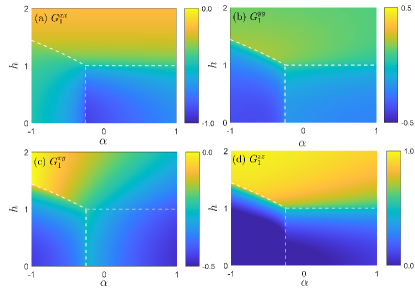
Figure 9: The contour map of correlation functions (a) $G_{1}^{xx}$, (b) $G_{1}^{yy}$, (c) $G_{1}^{xy}$ and (d) $G_{1}^{zz}$ with respect to $\alpha$ and $h$ with $N=2000$, $J=1.00$, $\Gamma=0.60,\gamma=0.60$. The white dashed lines correspond to the critical lines.

To be concrete, it is easy to calculate the nearest-neighbor correlations (i.e., $r=1$); we have

$$G_{i,i+1}^{xx} = \langle B_{i}A_{i+1}\rangle,\quad G_{i,i+1}^{yy}=-\langle A_{i}B_{i+1}\rangle,$$

$$G_{i,i+1}^{xy} = i\langle B_{i}B_{i+1}\rangle,\quad G_{i,i+1}^{yx}=i\langle A_{i}A_{i+1}\rangle,$$

$$G_{i,i+1}^{zz} = \langle A_{i}B_{i}A_{i+1}B_{i+1}\rangle$$

$$= \langle\sigma_{i}^{z}\rangle\langle\sigma_{i+1}^{z}\rangle\!-\!\langle\sigma_{i}^{x}\sigma_{i+1}^{x}\rangle\langle\sigma_{i}^{y}\sigma_{i+1}^{y}\rangle\!+\!\langle\sigma_{i}^{x}\sigma_{i+1}^{y}\rangle\langle\sigma_{i}^{y}\sigma_{i+1}^{x}\rangle.$$

The contour plots of nearest-neighbor correlation functions are shown in Fig. 9 and provide a full scope of Figs. 4 and 5. Similarly, the contour plot of the steered quantum coherence in Fig.10 complements the slice plot in Fig.7.

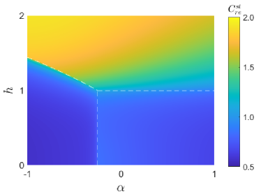
Figure 10: The contour map of steered quantum coherence $C_{re}^{st}$ with respect to $\alpha$ and $h$ with $N=2000$, $J=1.00$, $\Gamma=0.60,\gamma=0.60$. The white dashed lines correspond to the critical lines.

The four-qubit correlation is described by the $z$ component vector chiral order parameter [63, 64]

$$\kappa_{i}=\left(\sigma_{i}\times\sigma_{i+1}\right)^{z}.$$ (85)

As for the consecutive four qubits, it yields

$$\langle\kappa_{i}\kappa_{i+1}\rangle=\langle B_{i}B_{i+2}\rangle.$$ (86)

When the dimers are farther than the nearest neighbor, we have for $r\equiv j-i>1$

$$\langle\kappa_{i}\kappa_{j}\rangle = \langle B_{i}B_{j}\rangle\langle B_{i+1}B_{j+1}\rangle-\langle B_{i}B_{i+1}\rangle\langle B_{j}B_{j+1}\rangle$$ (87)

$$- \langle B_{i}B_{j+1}\rangle\langle B_{i+1}B_{j}\rangle.$$

It is recognized that the nonvanishing cross-correlations arouse nontrivial effect in reflection-symmetry-broken systems and lead to the gapless phase with quasi-long-range order.

References

- Sachdev [2008] S. Sachdev, Quantum magnetism and criticality, Nature Physics 4, 173 (2008).
- Mazurenko and Anisimov [2005] V. V. Mazurenko and V. I. Anisimov, Weak ferromagnetism in antiferromagnets: and , Phys. Rev. B 71, 184434 (2005).
- Fink and Shaltiel [1963] H. J. Fink and D. Shaltiel, High-frequency resonance of a weak ferromagnet: MnC, Phys. Rev. 130, 627 (1963).
- Zhang et al. [2021] Y. Zhang, J. Liu, Y. Dong, S. Wu, J. Zhang, J. Wang, J. Lu, A. Rückriegel, H. Wang, R. Duine, H. Yu, Z. Luo, K. Shen, and J. Zhang, Strain-driven dzyaloshinskii-moriya interaction for room-temperature magnetic skyrmions, Phys. Rev. Lett. 127, 117204 (2021).
- Liu et al. [2021a] X. Liu, W. Song, M. Wu, Y. Yang, Y. Yang, P. Lu, Y. Tian, Y. Sun, J. Lu, J. Wang, et al., Magnetoelectric phase transition driven by interfacial-engineered Dzyaloshinskii-Moriya interaction, Nature communications 12, 5453 (2021a).
- Muühlbauer et al. [2009] S. Muühlbauer, B. Binz, F. Jonietz, C. Pfleiderer, A. Rosch, A. Neubauer, R. Georgii, and P. Boöni, Skyrmion lattice in a chiral magnet, Science 323, 915 (2009).
- Yu et al. [2010] X. Yu, Y. Onose, N. Kanazawa, J. H. Park, J. Han, Y. Matsui, N. Nagaosa, and Y. Tokura, Real-space observation of a two-dimensional skyrmion crystal, Nature 465, 901 (2010).
- Katukuri et al. [2014] V. M. Katukuri, S. Nishimoto, V. Yushankhai, A. Stoyanova, H. Kandpal, S. Choi, R. Coldea, I. Rousochatzakis, L. Hozoi, and J. Van Den Brink, Kitaev interactions between moments in honeycomb are large and ferromagnetic: insights from ab initio quantum chemistry calculations, New Journal of Physics 16, 013056 (2014).
- Rau et al. [2014] J. G. Rau, E. K.-H. Lee, and H.-Y. Kee, Generic spin model for the honeycomb iridates beyond the kitaev limit, Phys. Rev. Lett. 112, 077204 (2014).
- Reuther et al. [2011] J. Reuther, R. Thomale, and S. Trebst, Finite-temperature phase diagram of the Heisenberg-Kitaev model, Phys. Rev. B 84, 100406 (2011).
- Trousselet et al. [2011] F. Trousselet, G. Khaliullin, and P. Horsch, Effects of spin vacancies on magnetic properties of the Kitaev-Heisenberg model, Phys. Rev. B 84, 054409 (2011).
- Ducatman et al. [2018] S. Ducatman, I. Rousochatzakis, and N. B. Perkins, Magnetic structure and excitation spectrum of the hyperhoneycomb Kitaev magnet , Phys. Rev. B 97, 125125 (2018).
- Smit et al. [2020] R. L. Smit, S. Keupert, O. Tsyplyatyev, P. A. Maksimov, A. L. Chernyshev, and P. Kopietz, Magnon damping in the zigzag phase of the Kitaev-Heisenberg- model on a honeycomb lattice, Phys. Rev. B 101, 054424 (2020).
- Takikawa and Fujimoto [2019] D. Takikawa and S. Fujimoto, Impact of off-diagonal exchange interactions on the Kitaev spin-liquid state of , Phys. Rev. B 99, 224409 (2019).
- Xu et al. [2020] C. Xu, J. Feng, M. Kawamura, Y. Yamaji, Y. Nahas, S. Prokhorenko, Y. Qi, H. Xiang, and L. Bellaiche, Possible kitaev quantum spin liquid state in 2d materials with S=, Phys. Rev. Lett. 124, 087205 (2020).
- Feynman [1982] R. Feynman, Simulating physics with computers, International Journal of Theoretical Physics 21, 467 (1982).
- Trotzky et al. [2008] S. Trotzky, P. Cheinet, S. Folling, M. Feld, U. Schnorrberger, A. M. Rey, A. Polkovnikov, E. A. Demler, M. D. Lukin, and I. Bloch, Time-resolved observation and control of superexchange interactions with ultracold atoms in optical lattices, Science 319, 295 (2008).
- Yan et al. [2013] B. Yan, S. A. Moses, B. Gadway, J. P. Covey, K. R. A. Hazzard, A. M. Rey, D. S. Jin, and J. Ye, Observation of dipolar spin-exchange interactions with lattice-confined polar molecules, Nature 501, 521 (2013).
- Jurcevic et al. [2014] P. Jurcevic, B. P. Lanyon, P. Hauke, C. Hempel, P. Zoller, R. Blatt, and C. F. Roos, Quasiparticle engineering and entanglement propagation in a quantum many-body system, Nature 511, 202 (2014).
- Richerme et al. [2014] P. Richerme, Z.-X. Gong, A. Lee, C. Senko, J. Smith, M. Foss-Feig, S. Michalakis, A. V. Gorshkov, and C. Monroe, Non-local propagation of correlations in quantum systems with long-range interactions, Nature 511, 198 (2014).
- Hung et al. [2016] C.-L. Hung, A. González-Tudela, J. I. Cirac, and H. J. Kimble, Quantum spin dynamics with pairwise-tunable, long-range interactions, Proc. Natl. Acad. Sci. 113, E4946 (2016).
- Douglas et al. [2015] J. S. Douglas, H. Habibian, C. L. Hung, A. V. Gorshkov, H. J. Kimble, and D. E. Chang, Quantum many-body models with cold atoms coupled to photonic crystals, Nature Photonics 9, 326 (2015).
- González-Tudela et al. [2015] A. González-Tudela, C. L. Hung, D. E. Chang, J. I. Cirac, and H. J. Kimble, Subwavelength vacuum lattices and atom–atom interactions in two-dimensional photonic crystals, Nature Photonics 9, 320 (2015).
- Browaeys and Lahaye [2020] A. Browaeys and T. Lahaye, Many-body physics with individually controlled Rydberg atoms, Nature Physics 16, 132 (2020).
- Ebadi et al. [2021] S. Ebadi, T. T. Wang, H. Levine, A. Keesling, G. Semeghini, A. Omran, D. Bluvstein, R. Samajdar, H. Pichler, W. W. Ho, et al., Quantum phases of matter on a 256-atom programmable quantum simulator, Nature 595, 227 (2021).
- Davis et al. [2020] E. J. Davis, A. Periwal, E. S. Cooper, G. Bentsen, S. J. Evered, K. Van Kirk, and M. H. Schleier-Smith, Protecting spin coherence in a tunable heisenberg model, Phys. Rev. Lett. 125, 060402 (2020).
- Chiocchetta et al. [2021] A. Chiocchetta, D. Kiese, C. P. Zelle, F. Piazza, and S. Diehl, Cavity-induced quantum spin liquids, Nature Communications 12, 5901 (2021).
- Glaetzle et al. [2015] A. W. Glaetzle, M. Dalmonte, R. Nath, C. Gross, I. Bloch, and P. Zoller, Designing frustrated quantum magnets with laser-dressed rydberg atoms, Phys. Rev. Lett. 114, 173002 (2015).
- Mivehvar et al. [2019] F. Mivehvar, H. Ritsch, and F. Piazza, Cavity-quantum-electrodynamical toolbox for quantum magnetism, Phys. Rev. Lett. 122, 113603 (2019).
- Mivehvar et al. [2021] F. Mivehvar, F. Piazza, T. Donner, and H. Ritsch, Cavity QED with quantum gases: new paradigms in many-body physics, Advances in Physics 70, 1 (2021).
- Gopalakrishnan et al. [2011] S. Gopalakrishnan, B. L. Lev, and P. M. Goldbart, Frustration and glassiness in spin models with cavity-mediated interactions, Phys. Rev. Lett. 107, 277201 (2011).
- Mivehvar et al. [2017] F. Mivehvar, F. Piazza, and H. Ritsch, Disorder-driven density and spin self-ordering of a bose-einstein condensate in a cavity, Phys. Rev. Lett. 119, 063602 (2017).
- Landini et al. [2018] M. Landini, N. Dogra, K. Kroeger, L. Hruby, T. Donner, and T. Esslinger, Formation of a spin texture in a quantum gas coupled to a cavity, Phys. Rev. Lett. 120, 223602 (2018).
- Ren et al. [2022] J. Ren, Z. Wang, W.-X. Chen, and W.-L. You, Long-range order and quantum criticality in antiferromagnetic chains with long-range staggered interactions, Phys. Rev. E 105, 034128 (2022).
- You [2009] W.-L. You, Long-range order in two-dimensional XXZ model, International Journal of Modern Physics B 23, 2195 (2009).
- Tang and Hirsch [1989] S. Tang and J. E. Hirsch, Long-range order without broken symmetry: Two-dimensional Heisenberg antiferromagnet at zero temperature, Phys. Rev. B 39, 4548 (1989).
- Lin and Campbell [1992] H. Q. Lin and D. K. Campbell, Long-range order in the 2D antiferromagnetic Heisenberg model: A renormalization perspective, Phys. Rev. Lett. 69, 2415 (1992).
- Li et al. [2021] Z. Li, S. Choudhury, and W. V. Liu, Long-range-ordered phase in a quantum Heisenberg chain with interactions beyond nearest neighbors, Phys. Rev. A 104, 013303 (2021).
- Dzyaloshinsky [1958] I. Dzyaloshinsky, A thermodynamic theory of “weak” ferromagnetism of antiferromagnetics, Journal of physics and chemistry of solids 4, 241 (1958).
- Anderson [1959] P. W. Anderson, New approach to the theory of superexchange interactions, Phys. Rev. 115, 2 (1959).
- Moriya [1960a] T. Moriya, Anisotropic superexchange interaction and weak ferromagnetism, Phys. Rev. 120, 91 (1960a).
- Moriya [1960b] T. Moriya, New mechanism of anisotropic superexchange interaction, Phys. Rev. Lett. 4, 228 (1960b).
- Luo et al. [2021a] Q. Luo, J. Zhao, X. Wang, and H.-Y. Kee, Unveiling the phase diagram of a bond-alternating spin- K chain, Phys. Rev. B 103, 144423 (2021a).
- Luo et al. [2021b] Q. Luo, S. Hu, and H.-Y. Kee, Unusual excitations and double-peak specific heat in a bond-alternating spin-1 K chain, Phys. Rev. Research 3, 033048 (2021b).
- Liu et al. [2020] Z.-A. Liu, T.-C. Yi, J.-H. Sun, Y.-L. Dong, and W.-L. You, Lifshitz phase transitions in a one-dimensional gamma model, Phys. Rev. E 102, 032127 (2020).
- Yang et al. [2020a] W. Yang, A. Nocera, T. Tummuru, H.-Y. Kee, and I. Affleck, Phase diagram of the spin- kitaev-gamma chain and emergent SU(2) symmetry, Phys. Rev. Lett. 124, 147205 (2020a).
- Sørensen et al. [2021] E. S. Sørensen, A. Catuneanu, J. S. Gordon, and H.-Y. Kee, Heart of entanglement: Chiral, nematic, and incommensurate phases in the Kitaev-Gamma ladder in a field, Phys. Rev. X 11, 011013 (2021).
- Yang et al. [2020b] W. Yang, A. Nocera, and I. Affleck, Comprehensive study of the phase diagram of the spin- Kitaev-Heisenberg-Gamma chain, Phys. Rev. Research 2, 033268 (2020b).
- Vaidya et al. [2018] V. D. Vaidya, Y. Guo, R. M. Kroeze, K. E. Ballantine, A. J. Kollár, J. Keeling, and B. L. Lev, Tunable-range, photon-mediated atomic interactions in multimode cavity qed, Phys. Rev. X 8, 011002 (2018).
- Guo et al. [2021] Y. Guo, R. M. Kroeze, B. P. Marsh, S. Gopalakrishnan, J. Keeling, and B. L. Lev, An optical lattice with sound, Nature 599, 211 (2021).
- Periwal et al. [2021] A. Periwal, E. S. Cooper, P. Kunkel, J. F. Wienand, E. J. Davis, and M. Schleier-Smith, Programmable interactions and emergent geometry in an array of atom clouds, Nature 600, 630 (2021).
- Bitko et al. [1996] D. Bitko, T. F. Rosenbaum, and G. Aeppli, Quantum critical behavior for a model magnet, Phys. Rev. Lett. 77, 940 (1996).
- Cui et al. [2019] Y. Cui, H. Zou, N. Xi, Z. He, Y. X. Yang, L. Shu, G. H. Zhang, Z. Hu, T. Chen, R. Yu, et al., Quantum criticality of the ising-like screw chain antiferromagnet in a transverse magnetic field, Phys. Rev. Lett. 123, 067203 (2019).
- Kenzelmann et al. [2002] M. Kenzelmann, R. Coldea, D. A. Tennant, D. Visser, M. Hofmann, P. Smeibidl, and Z. Tylczynski, Order-to-disorder transition in the -like quantum magnet induced by noncommuting applied fields, Phys. Rev. B 65, 144432 (2002).
- Coldea et al. [2010] R. Coldea, D. Tennant, E. Wheeler, E. Wawrzynska, D. Prabhakaran, M. Telling, K. Habicht, P. Smeibidl, and K. Kiefer, Quantum criticality in an Ising chain: experimental evidence for emergent symmetry, Science 327, 177 (2010).
- Faure et al. [2019] Q. Faure, S. Takayoshi, V. Simonet, B. Grenier, M. Månsson, J. S. White, G. S. Tucker, C. Rüegg, P. Lejay, T. Giamarchi, and S. Petit, Tomonaga-luttinger liquid spin dynamics in the quasi-one-dimensional Ising-like antiferromagnet , Phys. Rev. Lett. 123, 027204 (2019).
- Chauhan et al. [2020] P. Chauhan, F. Mahmood, H. J. Changlani, S. M. Koohpayeh, and N. P. Armitage, Tunable magnon interactions in a ferromagnetic spin-1 chain, Phys. Rev. Lett. 124, 037203 (2020).
- Yi et al. [2018] T.-C. Yi, Y.-R. Ding, J. Ren, Y.-M. Wang, and W.-L. You, Quantum coherence of XY model with Dzyaloshinskii-Moriya interaction, Acta Physica Sinica 67, 140303 (2018).
- Rufo et al. [2019] S. Rufo, N. Lopes, M. A. Continentino, and M. A. R. Griffith, Multicritical behavior in topological phase transitions, Phys. Rev. B 100, 195432 (2019).
- Su et al. [2006] S.-Q. Su, J.-L. Song, and S.-J. Gu, Local entanglement and quantum phase transition in a one-dimensional transverse field Ising model, Phys. Rev. A 74, 032308 (2006).
- Liu et al. [2021b] Z.-A. Liu, Y.-L. Dong, N. Wu, Y. Wang, and W.-L. You, Quantum criticality and correlations in the Ising-Gamma chain, Physica A: Statistical Mechanics and its Applications 579, 126122 (2021b).
- Barouch and McCoy [1971] E. Barouch and B. M. McCoy, Statistical mechanics of the model. II. spin-correlation functions, Phys. Rev. A 3, 786 (1971).
- McCulloch et al. [2008] I. P. McCulloch, R. Kube, M. Kurz, A. Kleine, U. Schollwöck, and A. K. Kolezhuk, Vector chiral order in frustrated spin chains, Phys. Rev. B 77, 094404 (2008).
- Ueda and Onoda [2014] H. Ueda and S. Onoda, Vector-spin-chirality order in a dimerized frustrated spin- chain, Phys. Rev. B 89, 024407 (2014).
- Vidal et al. [2003] G. Vidal, J. I. Latorre, E. Rico, and A. Kitaev, Entanglement in quantum critical phenomena, Phys. Rev. Lett. 90, 227902 (2003).
- Osterloh et al. [2002] A. Osterloh, L. Amico, G. Falci, and R. Fazio, Scaling of entanglement close to a quantum phase transition, Nature 416, 608 (2002).
- Gu et al. [2003] S.-J. Gu, H.-Q. Lin, and Y.-Q. Li, Entanglement, quantum phase transition, and scaling in the chain, Phys. Rev. A 68, 042330 (2003).
- Ollivier and Zurek [2001] H. Ollivier and W. H. Zurek, Quantum discord: A measure of the quantumness of correlations, Phys. Rev. Lett. 88, 017901 (2001).
- Modi et al. [2012] K. Modi, A. Brodutch, H. Cable, T. Paterek, and V. Vedral, The classical-quantum boundary for correlations: Discord and related measures, Rev. Mod. Phys. 84, 1655 (2012).
- Chen et al. [2016] J.-J. Chen, J. Cui, Y.-R. Zhang, and H. Fan, Coherence susceptibility as a probe of quantum phase transitions, Phys. Rev. A 94, 022112 (2016).
- You et al. [2007] W.-L. You, Y.-W. Li, and S.-J. Gu, Fidelity, dynamic structure factor, and susceptibility in critical phenomena, Phys. Rev. E 76, 022101 (2007).
- Bloch [2008] I. Bloch, Quantum coherence and entanglement with ultracold atoms in optical lattices, Nature 453, 1016 (2008).
- Baumgratz et al. [2014] T. Baumgratz, M. Cramer, and M. B. Plenio, Quantifying coherence, Phys. Rev. Lett. 113, 140401 (2014).
- You et al. [2017] W.-L. You, C.-J. Zhang, W. Ni, M. Gong, and A. M. Oleś, Emergent phases in a compass chain with multisite interactions, Phys. Rev. B 95, 224404 (2017).
- You et al. [2018] W.-L. You, Y. Wang, T.-C. Yi, C. Zhang, and A. M. Oleś, Quantum coherence in a compass chain under an alternating magnetic field, Phys. Rev. B 97, 224420 (2018).
- Yi et al. [2019] T.-C. Yi, W.-L. You, N. Wu, and A. M. Oleś, Criticality and factorization in the Heisenberg chain with Dzyaloshinskii-Moriya interaction, Phys. Rev. B 100, 024423 (2019).
- Hu and Fan [2018] M.-L. Hu and H. Fan, Nonlocal advantage of quantum coherence in high-dimensional states, Phys. Rev. A 98, 022312 (2018).
- Hu et al. [2020] M.-L. Hu, Y.-Y. Gao, and H. Fan, Steered quantum coherence as a signature of quantum phase transitions in spin chains, Phys. Rev. A 101, 032305 (2020).
- Hu et al. [2021] M.-L. Hu, F. Fang, and H. Fan, Finite-size scaling of coherence and steered coherence in the lipkin-meshkov-glick model, Phys. Rev. A 104, 062416 (2021).
- Sinha et al. [2019] A. Sinha, M. M. Rams, and J. Dziarmaga, Kibble-Zurek mechanism with a single particle: Dynamics of the localization-delocalization transition in the Aubry-André model, Phys. Rev. B 99, 094203 (2019).
- Chepiga and Mila [2021] N. Chepiga and F. Mila, Kibble-Zurek exponent and chiral transition of the period-4 phase of Rydberg chains, Nature Communications 12, 414 (2021).