Anderson acceleration with approximate calculations: applications to scientific computing

Abstract

We provide rigorous theoretical bounds for Anderson acceleration (AA) that allow for efficient approximate residual calculations in AA, which in turn reduce computational time and memory storage while maintaining convergence. Specifically, we propose a reduced variant of AA, which consists in projecting the least-squares used to compute the Anderson mixing onto a subspace of reduced dimension. The dimensionality of this subspace adapts dynamically at each iteration as prescribed by computable heuristic quantities guided by rigorous theoretical error bounds. The use of heuristics to monitor the error introduced by approximate calculations, combined with the check on monotonicity of the convergence, ensures the convergence of the numerical scheme within a prescribed tolerance threshold on the residual. We numerically show and assess the performance of AA with approximate calculations on: (i) linear deterministic fixed-point iterations arising from the Richardson’s scheme to solve linear systems with open-source benchmark matrices with various preconditioners and (ii) non-linear deterministic fixed-point iterations arising from non-linear time-dependent Boltzmann equations.

65F10, 65F50, 65G30, 65G50, 65N12, 65N15, 65Y20, 65Z05, 68T01, 68W20, 68W40

1 Introduction

Efficient fixed-point schemes are needed in many complex physical applications such as: (i) iterative algorithms to solve sparse linear systems, (ii) Picard iterations [12] to solve systems of non-linear partial differential equations as in computational fluid dynamics [17, 33], semiconductor modelling [15, 25], and astrophysics [27, 26], and (iii) solving extended-space full-waveform inversion (FWI) [1].

For scientific applications, the standard fixed-point scheme often converges slowly either because the fixed-point operator is either weakly globally contractive or is not globally contractive at all. The Anderson acceleration (AA) [2] is a multi-secant method [9, 7] that has been widely used either to improve the convergence rate of convergent fixed-point schemes or to restore convergence when the original fixed-point scheme is not convergent [18, 45, 34, 46, 8]. In particular, the convergence of AA has been studied with respect to specific properties of different scientific applications [43, 42, 29, 5].

AA requires solving a least-squares problem at each fixed-point iteration, and this can be computationally expensive for scientific applications that involve large-scale calculations, especially when such calculations are distributed on high-performance computing (HPC) platforms. To reduce the computational cost of AA, a recently proposed variant of AA called Alternating Anderson Richardson (AAR) [3, 36, 41] performs multiple fixed-point iterations between two consecutive Anderson mixing corrections. In particular, the number of fixed-point iterations between two consecutive Anderson mixing corrections can be arbitrarily set by the user. When the number is set to one, AAR reduces back to AA. Recent theoretical results have shown that AAR is more robust than the standard AA against stagnations [28]. However, even if performed intermittently, computing the Anderson mixing via least-squares can still be computationally expensive when the number of rows in the tall and skinny matrix that defines the left-hand side (LHS) of the least-squares problem is large. One possibility to reduce the computational cost is to perform approximate/inexact calculations in the AAR scheme. To avoid compromising the convergence of AAR, the computation accuracy reduction must be performed judiciously. For specific problems, the accuracy has been reduced by projecting the least-squares problem in the Anderson mixing computation onto an appropriate projection subspace, which results in computational savings without affecting the final convergence of the fixed-point scheme [20, 31]. In these approaches, the accuracy reduction has been controlled by using physics information about the problem at hand to identify an effective projection subspace. However, physics-driven guidelines are difficult (and often impossible) to determine because of the lack of structure in the fixed-point operator. In this situation, general guidelines (not necessarily physics driven) to judiciously reduce the accuracy in solving the least-squares problem are needed.

We provide rigorous theoretical bounds for AAR on linear fixed-point iterations that establish general guidelines to reduce the accuracy of the calculations performed by AAR while still ensuring that the final residual of the fixed-point scheme drops below a user-defined convergence threshold. By interpreting the accuracy reduction in AAR calculations as a perturbation to the original least-squares problem in the Anderson mixing computation, we assess how much accuracy can be sacrificed to limit the communication and computational burden without compromising convergence. Along the same lines as previously published theoretical results in [40] for well-established Krylov methods [37], our analysis concludes that the convergence of AAR can be maintained while allowing to progressively reduce the accuracy for the calculations within the AAR scheme.

Our theoretical results allow for accuracy reduction in different calculations performed by AAR. When the fixed-point operator evaluations are the dominant computation cost of AAR, one may choose to perform approximate evaluations. When instead solving the least-squares problem for the Anderson mixing is the most expensive step of AAR, one may solve the least-squares problem approximately. These theoretical results open a new path to efficiently apply AAR to solve problems in addition to sparse linear systems, including non-linear fixed-point iterations arising from quantum mechanics, plasma astrophysics, and computational fluid dynamics where fixed-point operator evaluations are often expensive [42]. In this context, the use of AAR allows to leverage less expensive operator evaluations without affecting the final attainable accuracy of the non-linear physics solver.

Since the theoretical bounds are defined in terms of quantities that are not always easily computable, we also propose heuristics that are inexpensive to compute while still maintaining a close relation to the rigorous theoretical estimates. The heuristics allow to dynamically adjust the accuracy in the AAR calculations without introducing additional computational overhead. We combine the heuristics with a check on the monotonic reduction of the residual norm across two consecutive Anderson mixing steps to ensure that the accuracy reduction in the AAR calculations does not compromise the convergence of the numerical scheme. The monotonicity check allows one to replace the tight theoretical bound with an empirical one, and dynamically tighten the tolerance of inexact calculations if non-monotonicity of the residual norm is observed across two consecutive AA steps.

In the numerical sections, we assess the effectiveness of our heuristics using two different approaches to inject inaccuracies into AAR. The first approach injects error in the evaluations of the fixed-point operator, and the heuristics are used to dynamically adjust the magnitude of the error injected. The second approach projects the least-squares problem in the Anderson mixing computation onto a subspace, and the heuristics are used to dynamically adjust the dimension of projection subspace. Numerical results confirm that using approximate calculations to solve the least-squares problem for AA saves computational time without sacrificing convergence to a desired accuracy. The proposed method has appealing properties for HPC since it reduces computational requirements, inter-process communications, and storage requirements to solve least-squares problem in AA when the fixed-point operator is distributed across multi-node processors.

The remainder of the paper is organized as follows. In Section 2.2 we briefly recall the stationary Richardson’s method that solves linear systems by recasting them as linear fixed-point iterations. In Section 3 we provide error bounds that allow approximate calculations of AA for linear fixed-point iterations while still maintaining convergence. In Section 4 we introduce the new formulation of AAR that enables the projection of the least-squares problem onto a projection subspace, called Reduced AAR, followed in Section 5 by numerical implementations of the analyses conducted in the previous sections for two different scientific applications that we use as representatives of two different types of fixed-point iterations. The applications we consider are: (i) linear deterministic fixed-point iterations arising from the Richardson’s scheme to solve linear systems and (ii) non-linear deterministic fixed-point iterations arising from non-linear time-dependent Boltzmann equations. We conclude the paper with remarks on the state-of-the-art and comments about future developments in Section 6.

2 Fixed-point iteration

The standard iterative method for solving a fixed-point problem $\mathbf{x}=G(\mathbf{x})$ with $\mathbf{x}\in\mathbb{R}^{n}$ and $G:\mathbb{R}^{n}\rightarrow\mathbb{R}^{n}$ is the fixed-point iteration:

(1) $$\mathbf{x}^{k+1}=G(\mathbf{x}^{k}),\quad k=0,1,\ldots,$$

and the residual $\mathbf{r}^{k}\in\mathbb{R}^{n}$ of the fixed-point iteration is defined as

(2) $$\mathbf{r}^{k}=G(\mathbf{x}^{k})-\mathbf{x}^{k},\quad k=0,1,\ldots\>.$$

The convergence of the fixed-point iteration relies on the global contraction property of the nonlinear fixed-point operator $G$, i.e., there is a constant $c<1$ such that, for every $\mathbf{x}\in\mathbb{R}^{n}$ and $\mathbf{y}\in\mathbb{R}^{n}$, $\lVert G(\mathbf{x})-G(\mathbf{y})\rVert_{2}\leq c\lVert\mathbf{x}-\mathbf{y}\rVert_{2}$. When such $c$ is close to one, the fixed-point iteration may converge at an unacceptably slow rate.

2.1 Anderson acceleration and the Alternating Anderson acceleration

The AA was proposed in [2] to accelerate the fixed-point iteration. There exist several equivalent formulations of AA [18, 43]. The formulation we adopt for convenience in the analysis is described in Algorithm 1. Define

(3) $$X_{k}=[(\mathbf{x}^{k-\ell+1}-\mathbf{x}^{k-\ell}),\ldots,(\mathbf{x}^{k}-\mathbf{x}^{k-1})]\in\mathbb{R}^{n\times\ell}$$

and

(4) $$R_{k}=[(\mathbf{r}^{k-\ell+1}-\mathbf{r}^{k-\ell}),\ldots,(\mathbf{r}^{k}-\mathbf{r}^{k-1})]\in\mathbb{R}^{n\times\ell},$$

where $\ell=\min\{k,m\}$ and $m$ is an integer that describes the maximum number of previous terms of the sequence $\{\mathbf{x}^{k}\}_{k=0}^{\infty}$ used to compute the AA update. Denoting with $\lVert\cdot\rVert_{2}$ the $\ell^{2}$-norm of a vector, the vector $\mathbf{g}^{k}=[g^{(k)}_{1},\ldots,g^{(k)}_{\ell}]^{T}\in\mathbb{R}^{\ell}$ defined as

(5) $$\mathbf{g}^{k}=\underset{\mathbf{g}\in\mathbb{R}^{\ell}}{\operatorname{argmin}}\lVert R_{k}\mathbf{g}-\mathbf{r}^{k}\rVert_{2}^{2}$$

is used to update the sequence $\{\mathbf{x}^{k}\}_{k=0}^{\infty}$ through an Anderson mixing as follows

(6) $$\mathbf{x}^{k+1}=\mathbf{x}^{k}+{\mathbf{r}^{k}}-(X_{k}+R_{k})\mathbf{g}^{k}.$$

Algorithm 1 (Alternating) Anderson Acceleration

  Data: $\mathbf{x}^{0}\in\mathbb{R}^{n}$, $p\in\mathbb{N}$; {$//\texttt{AA: }p=1,\,\,\texttt{Alternating AA: }p>1$}

  Compute $\mathbf{r}^{0}=G(\mathbf{x}^{0})-\mathbf{x}^{0}$ and $\mathbf{x}^{1}=\mathbf{x}^{0}+\mathbf{r}^{0}$;

  Set $k=1$

  while $\displaystyle\lVert\mathbf{r}^{k-1}\rVert_{2}>tol$ do

     Compute $\ell=\min\{k,m\}$

     Compute $\mathbf{r}^{k}=G(\mathbf{x}^{k})-\mathbf{x}^{k}$

     if $k\pmod{p}\neq 0$ then

        Update $\mathbf{x}^{k+1}=\mathbf{x}^{k}+\omega\mathbf{r}^{k}$

     else

        Set $X_{k}=[(\mathbf{x}^{k-\ell+1}-\mathbf{x}^{k-\ell}),\ldots,(\mathbf{x}^{k}-\mathbf{x}^{k-1})]\in\mathbb{R}^{n\times\ell}$

         Set $R_{k}=[(\mathbf{r}^{k-\ell+1}-\mathbf{r}^{k-\ell}),\ldots,(\mathbf{r}^{k}-\mathbf{r}^{k-1})]\in\mathbb{R}^{n\times\ell}$

        Compute $\displaystyle\mathbf{g}^{k}=\underset{\mathbf{g}\in\mathbb{R}^{\ell}}{\operatorname{argmin}}\lVert R_{k}\mathbf{g}-\mathbf{r}^{k}\rVert_{2}^{2}$

        Update ${\mathbf{x}^{k+1}=\mathbf{x}^{k}+\mathbf{r}^{k}-(X_{k}+R_{k})\mathbf{g}^{k}}$.

     end if

     $k=k+1$

  end while

  return  $\mathbf{x}^{k+1}$

When compared to the fixed-point iteration, AA often requires fewer iterations to converge thus resulting in a shorter computational time. On the other hand, AA also introduces the overhead of solving the least-squares problem (5) at each iteration. This computation overhead is outweighed by the benefit from fewer iterations when solving problems in which evaluating the operator $G$ incurs the dominant cost. However, there are many problems where the cost of solving this least-squares problem incurs the main cost.

Solving a least-squares problem at each iteration is computationally expensive and requires global communications which introduce severe bottlenecks for the parallelization in HPC environments. P. Suryanarayana and collaborators [41] recently proposed to compute an Anderson mixing after multiple Picard iterations, so that the cost of solving successive least-squares problems is reduced. This new AA variant, called Alternating AA, has been shown to effectively accelerate both linear and non-linear fixed-point iterations [36, 41]. Algorithm 1 describes the Alternating AA, where the parameter $p$ represents the number of Picard iterations separating two consecutive AA steps. Letting $p\rightarrow\infty$ reduces the Alternating AA to a standard fixed-point scheme with $\omega$ the relaxation parameter, while $p=1$ makes it coincide with the standard AA formulation.

In sections 2.2 and 2.3 we focus on the case when $G$ is linear and arises from iteratively solving a sparse linear system.

2.2 Stationary Richardson

Consider a nonsingular sparse linear system

(7) $$A\mathbf{x}=\mathbf{b},$$

where $A\in\mathbb{R}^{n\times n}$ and $\mathbf{x}$, $\mathbf{b}\in\mathbb{R}^{n}$. We assume that left preconditioning has already been applied. Let $H:=I-A$; adding $H\mathbf{x}$ on both sides of (7) leads to a linear fixed-point problem with the fixed-point iteration

(8) $$\mathbf{x}^{k+1}=G(\mathbf{x}^{k}):=H\mathbf{x}^{k}+\mathbf{b},\quad k=0,1,\ldots\>.$$

A commonly used equivalent representation of (8) is the correction form

(9) $$\mathbf{x}^{k+1}=\mathbf{x}^{k}+\mathbf{r}^{k},\quad k=0,1,\ldots,$$

where $\mathbf{r}^{k}=\mathbf{b}-A\mathbf{x}^{k}$ is the residual at the $k$th iteration. The scheme (9) converges to the solution if and only if the spectral radius $\rho(H)<1$. The scheme (8) can be generalized by introducing a positive weighing parameter $\omega$:

(10) $$\mathbf{x}^{k+1}=(1-\omega)\mathbf{x}^{k}+\omega(H\mathbf{\mathbf{x}}^{k}+\mathbf{b}),$$

which in correction form is equivalently represented as

(11) $$\mathbf{x}^{k+1}=\mathbf{x}^{k}+\omega\mathbf{r}^{k}.$$

Equations (10) and (11) are known as the stationary Richardson scheme. It is also straightforward to verify that Equations (10) and (11) are equivalent to applying the fixed-point iteration to the linear operator $G_{\omega}(\mathbf{x}):=(I-\omega A)\mathbf{x}+\omega\mathbf{b}$.

2.3 Anderson acceleration for linear systems

The AA is well suited to potentially accelerate Richardson schemes. In the case of a linear fixed-point iteration as in Equation (8), AA can be split into two steps. The first step consists in calculating the Anderson mixing

(12) $$\overline{\mathbf{x}}^{k}=\mathbf{x}^{k}-X_{k}\mathbf{g}^{k},$$

where the vector $\mathbf{g}^{k}$ is computed by solving the over-determined least-squares problem in Equation (5). Under the assumption that $R_{k}$ is full rank, we have $\mathbf{g}^{k}=(R^{T}_{k}R_{k})^{-1}R^{T}_{k}\mathbf{r}^{k}$. Since $R_{k}=-AX_{k}$ for a linear fixed-point iteration, (12) can be recast as

(13) $$\overline{\mathbf{x}}^{k}=\mathbf{x}^{k}-X_{k}(R^{T}_{k}R_{k})^{-1}R^{T}_{k}\mathbf{r}^{k}=\mathbf{x}^{k}+X_{k}(R^{T}_{k}AX_{k})^{-1}R^{T}_{k}\mathbf{r}^{k}.$$

Therefore, the Anderson mixing can be interpreted as a step of an oblique projection method (see Chapter 5 of [38]) with the subspace of corrections chosen as $\mathcal{V}_{k}=\mathcal{R}(X_{k})$ and the subspace of constraints as $\mathcal{W}_{k}=\mathcal{R}(R_{k})=A\mathcal{R}(X_{k})=A\mathcal{V}_{k}$. After the Anderson mixing is applied, $\overline{\mathbf{x}}^{k}$ is used to compute a new update via a standard Richardson’s step

(14) $$\mathbf{x}^{k+1}=\overline{\mathbf{x}}^{k}+\omega\overline{\mathbf{r}}^{k},$$

where $\overline{\mathbf{r}}^{k}=\mathbf{b}-A\overline{\mathbf{x}}^{k}$. It can be shown that the iterative scheme from Equations (12) and (14) is equivalent to applying the standard Anderson mixing (6) to a fixed-point problem with operator $G_{\omega}(\mathbf{x}):=(I-\omega A)\mathbf{x}+\omega\mathbf{b}$. If AA is applied at each fixed-point iteration ($p=1$), this scheme is called Anderson-Richardson (AR) [2, 35, 44]. Studies about AR have highlighted similarities between this method and GMRES [18, 19, 35, 45]. When $p>1$, we refer to this approach as AAR. Recent studies have shown also that AAR is more robust against stagnations than AR [28].

2.3.1 Computational cost of AAR

Denoting the average number of non-zero entries per row of a sparse $n\times n$ matrix as $a$ and assuming for simplicity that this number is roughly constant across the rows, the computational complexity of a sparse matrix-vector multiplication is $\mathcal{O}(an)$. The least-squares problem in Equation (5) used to perform AA is solved using the QR factorization [21] of the $n\times m$ matrix $R_{k}$. The main components used in Algorithm 1 to perform AA with their computational costs expressed with the big-$\mathcal{O}$ are:

• QR factorization to perform AA: $\mathcal{O}(nm^{2})$

• matrix-vector multiplication: $\mathcal{O}(an)$.

AAR mitigates the computational cost to perform an AA step by interleaving successive AA step with $p$ relaxation sweeps. Relaxing the frequency at which the least-squares problem for AA is performed reduces the computational cost per iteration, but it is recommend not to excessively relax the frequency to avoid severely deteriorating the convergence rate of the overall numerical scheme. In practice, $p$ is often set to a value between 3 and 6 [28]. The average computational complexity of AAR is

(15) $$\mathcal{O}\bigg{(}an+\frac{1}{p}nm^{2}\bigg{)}.$$

We can see the $\frac{1}{p}$ factor in front of the computational cost of the QR factorization allows to mitigate the impact that the least-squares solve has over the total computational cost of the numerical scheme.

In large-scale distributed computational environments, solving the global least-squares problem at periodic intervals may still not be sufficient to avoid severe bottlenecks in the computation. Further reducing the computational cost to solve the least-squares problem is possible by replacing expensive and accurate calculations with inexpensive approximate ones while ensuring that convergence is maintained. To this end, in the following section we conduct an error analysis that provides theoretical bounds to estimate the error affordable at each iteration of AAR, which will allow us to develop numerical strategies to reduce the cost of the least-squares solves.

3 Backward stability analysis of approximate least-squares solves for AAR

The solution obtained by solving approximately the least-squares problem (5) can be treated as the exact solution of a different least-squares problem, which can be looked at as a yet unknown perturbation of the original problem (5). The object of this section is to estimate the difference between the original least-squares problem (5) and its perturbation. This is important in order to ensure backward stability [23, 24], which is a property of the numerical scheme to solve a problem as opposed to the forward stability, which is a property of the problem itself. Approximate calculations may arise from approximate evaluations of the fixed-point operator or from approximate calculations in the solver for the least-squares problem (5).

Analogous to the approach adopted in [28], we provide the backward stability analysis under the assumption that the AAR is not truncated, i.e., $m=k$, which henceforth we refer to as “Full AAR”. We focus on the backward stability analysis of Full AAR in the case that the mixing coefficients $\mathbf{g}^{k}$ solves an inexact or perturbed version of (5). Specifically, we consider the following two cases: (i) when backward perturbations are permitted only to the matrix $R_{k}$ on the left-hand side (LHS) of the least-squares system, which covers the scenario when the numerical methods performs an approximate factorization of $R_{k}$ (e.g., approximate QR or low-rank singular value decomposition), and (ii) when backward perturbations are permitted to both the LHS matrix $R_{k}$ and the residual vector $\mathbf{r}^{k}$ on the right-hand side (RHS), which occurs when matrix-vector multiplications are performed inexactly and/or the least-squares problem (5) is approximated by projection onto a subspace. The backward stability analyses for cases (i) and (ii) are given in Sections 3.1 and 3.2, respectively.

Let us denote with $\mathcal{E}_{k}\in\mathbb{R}^{n\times k}$ any perturbation to the matrix $R_{k}$ and $\delta\mathbf{r}_{k}\in\mathbb{R}^{n}$ any perturbation to the residual $\mathbf{r}^{k}$. The $i$th column of $\mathcal{E}_{k}$ can be modeled as an error matrix $E_{i}\in\mathbb{R}^{n\times n}$ applied to the $i$th columns of $R_{k}$, i.e.,

(16) $$\mathcal{E}_{k}=[E_{1}{(\mathbf{r}^{1}-\mathbf{r}^{0})},\ldots,E_{k}{(\mathbf{r}^{k}-\mathbf{r}^{k-1})}]\>.$$

We then denote the perturbed LHS as

(17) $$\hat{R}_{k}=R_{k}+\mathcal{E}_{k}=R_{k}+[E_{1}{(\mathbf{r}^{1}-\mathbf{r}^{0})},\ldots,E_{k}{(\mathbf{r}^{k}-\mathbf{r}^{k-1})}].$$

Using $\mathbf{r}^{i}-\mathbf{r}^{i-1}=-A(\mathbf{x}^{i}-\mathbf{x}^{i-1})$ for $i=1,\ldots,k$, we obtain

(18) $$\hat{R}_{k}=R_{k}{-}[E_{1}{A}(\mathbf{x}^{1}-\mathbf{x}^{0}),\ldots,E_{k}{A}(\mathbf{x}^{k}-\mathbf{x}^{k-1})].$$

As for the perturbed RHS, we denote it as

(19) $$\hat{\mathbf{r}}^{k}=\mathbf{r}^{k}+\delta\mathbf{r}^{k}\>.$$

To carry out the backward stability analysis in the following sections, we make the following assumption which will remain valid for the remainder of this paper.

Assumption 1.

The matrix $R_{k}$ is full rank, and the perturbation $\mathcal{E}_{k}$ does not compromise the full-rank property of $\hat{R}_{k}$.

In [28], the full-rank property of $R_{k}$ is not needed to ensure convergence of Full AAR. However, we need this property in the following theoretical analysis in order to ensure backward stability. According to [28], requiring that $R_{k}$ is full-rank already excludes the risk of stagnation. The same reasoning applies when $R_{k}$ is replaced by $\hat{R}_{k}$ to allow for inaccuracy in the least-squares calculations.

We denote the QR factorizations [22] of $R_{k}$ and $\hat{R}^{k}$ computed with a backward stable numerical method such as modified Gram-Schmidt or Householder transformations respectively as

(20) $$R_{k}=Q_{k}T_{k}\quad\text{and}\quad\hat{R}_{k}=\hat{Q}_{k}\hat{T}_{k},$$

where $Q_{k}\in\mathbb{R}^{n\times k}$ and $\hat{Q}_{k}\in\mathbb{R}^{n\times k}$ are matrices with orthogonal columns and $T_{k}\in\mathbb{R}^{k\times k}$ and $\hat{T}_{k}\in\mathbb{R}^{k\times k}$ are upper triangular matrices.

3.1 Backward stability analysis of AAR with perturbed LHS

In this subsection, we consider the case where the vector of mixing coefficients $\mathbf{g}^{k}$ in (12) is approximated by the solution ${\hat{\mathbf{g}}^{k}}$ of a perturbed least-squares problem

(21) $${\hat{\mathbf{g}}^{k}}=\underset{\mathbf{g}\in\mathbb{R}^{k}}{\operatorname{argmin}}\lVert\hat{R}_{k}\mathbf{g}-\mathbf{r}^{k}\rVert_{2}^{2},$$

where the perturbed LHS matrix $\hat{R}_{k}$ is defined in (18). The optimal backward error of the least-squares in (21) is defined as [23]

(22) $$\min_{\mathcal{E}_{k}}\{\lVert\mathcal{E}_{k}\rVert_{F}\;\text{:}\;\lVert(R_{k}+\mathcal{E}_{k}){\hat{\mathbf{g}}^{k}}-\mathbf{r}^{k}\rVert_{2}^{2}=\min\},$$

where $\lVert\cdot\rVert_{F}$ denotes the Frobenius norm. Denote with $z$ a positive integer. When the Anderson mixing is performed at iteration $k=zp$, we define the perturbation from the backward error as

(23) $$\delta_{k}=\|\mathcal{E}_{k}{\hat{\mathbf{g}}^{k}}\|_{2}=\lVert[E_{1}{A}(\mathbf{x}^{1}-\mathbf{x}^{0}),\ldots,E_{k}{A}(\mathbf{x}^{k}-\mathbf{x}^{k-1})]{{\hat{\mathbf{g}}^{k}}}\rVert_{2}.$$

Assume that $k={z}p$ iterations of the AAR have been carried out with approximate residual evaluations. The perturbation $\delta_{k}$ is bounded by

(24) $$\delta_{k}\leq\sum_{i=1}^{k}\lvert{\hat{g}_{i}}^{(k)}\rvert\lVert E_{i}\rVert_{2}{\lVert A\rVert_{2}}\lVert\mathbf{x}^{i}-\mathbf{x}^{i-1}\rVert_{2},$$

where $\lVert\cdot\rVert_{2}$ denotes the matrix norm induced by the $\ell^{2}$-norm of a vector. Given $\epsilon\in(0,1)$, we consider the perturbation matrices $E_{1},\ldots,E_{k}$ that satisfy the following chain of inequalities:

(25) $$\lVert[E_{1}{A}(\mathbf{x}^{1}-\mathbf{x}^{0}),\ldots,E_{k}{A}(\mathbf{x}^{k}-\mathbf{x}^{k-1})]\rVert_{2}\leq\epsilon{\lVert A\rVert_{2}}\lVert X_{k}\rVert_{2}\leq\sum_{i=1}^{k}\epsilon{\lVert A\rVert_{2}}\lVert\mathbf{x}^{i}-\mathbf{x}^{i-1}\rVert_{2}.$$

To simplify the presentation, we shall incorporate the norm of $A$ in the tolerance, thus defining $\varepsilon=\epsilon\lVert A\rVert_{2}$, $\varepsilon\in(0,\lVert A\rVert_{2})$. The following theoretical results provide error bounds on the affordable perturbation introduced into the least-squares problem by approximate calculations to ensure that the residuals of AAR iterates on the linear system (7) decreases below a user-defined threshold $\epsilon$.

Lemma 3.1.

Assume that $k={z}p$ iterations of Full AAR have been carried out. Let ${\hat{\mathbf{g}}}^{k}$ be the Anderson mixing computed by solving the perturbed least-squares problem defined in Equation (21). Then, the following inequality holds

(26) $$\lvert{\hat{g}}_{i}^{(k)}\rvert\leq\frac{1}{\sigma_{\min}(\hat{T}_{k})}\lVert\mathbf{r}^{k}\rVert_{2}\quad\text{for any}\quad i=1,\ldots,k.$$

Proof 3.2.

Let us denote with $\mathbf{r}^{k}_{\text{proj}}$ the $\ell^{2}$-orthogonal projection of the residual $\mathbf{r}^{k}$ onto the column space of $\hat{R}_{k}$. The use of the projected residual allows to recast the perturbed least-squares problem in Equation (21) as $\hat{R}_{k}{\hat{\mathbf{g}}^{k}}={\mathbf{r}^{k}_{\text{proj}}}$. By replacing the matrix $\hat{R}_{k}$ with its factorization $\hat{R}_{k}=\hat{Q}_{k}\hat{T}_{k}$ in the least-squares problem and applying $(\hat{T}_{k})^{-1}\hat{Q}_{k}^{T}$ on both sides of ${\hat{R}_{k}\hat{\mathbf{g}}^{k}}={\mathbf{r}^{k}_{\text{proj}}}$, we obtain

(27) $${\hat{\mathbf{g}}^{k}}=(\hat{T}_{k})^{-1}\hat{Q}_{k}^{T}{\mathbf{r}^{k}_{\text{proj}}}.$$

Then it follows that

(28) $$\lVert{\hat{\mathbf{g}}^{k}}\rVert_{2} =\lVert(\hat{T}_{k})^{-1}\hat{Q}_{k}^{T}{\mathbf{r}^{k}_{\text{proj}}}\rVert_{2}\leq\lVert(\hat{T}_{k})^{-1}\rVert_{2}\lVert\hat{Q}_{k}^{T}{\mathbf{r}^{k}_{\text{proj}}}\rVert_{2}=\lVert(\hat{T}_{k})^{-1}\rVert_{2}\lVert{\mathbf{r}^{k}_{\text{proj}}}\rVert_{2}$$

where the last equality is obtained using the property of orthogonal matrices acting as isometric transformations. The property of the projection operator always ensures that $\lVert\mathbf{r}^{k}_{\text{proj}}\rVert_{2}\leq\lVert\mathbf{r}^{k}\rVert_{2}$, thus allowing the following step

(29) $$\lVert{\hat{\mathbf{g}}^{k}}\rVert_{2}\leq\lVert(\hat{T}_{k})^{-1}\rVert_{2}\lVert\mathbf{r}^{k}\rVert_{2}.$$

Since $\lvert{\hat{g}_{i}^{(k)}}\rvert\leq\lVert{\hat{\mathbf{g}}^{k}}\rVert_{2}$ for $i=1,\ldots,k,$ and

(30) $$\lVert(\hat{T}_{k})^{-1}\rVert_{2}=\left({\sigma_{\min}(\hat{T}_{k})}\right)^{-1}$$

with $\sigma_{\min}(\hat{T}_{k})$ the smallest non-zero singular value of $\hat{T}_{k}$, the lemma follows.

Lemma 3.1 supports the demonstration of the following theorem, which provides a dynamic criterion for adjusting the accuracy of linear algebra operations that involve the matrix $\hat{R}_{k}$ in solving the least-squares, thus allowing for less expensive computations to solve (21), while maintaining accuracy.

Theorem 3.3.

Let $\epsilon>0$ and $\varepsilon=\epsilon\lVert A\rVert_{2}$. Let $\mathbf{r}^{k}$ be the residual of AAR after $k$ iterations. Assume that $k={z}p$ iterations of Full AAR have been carried out. If for every $i\leq k$,

(31) $$\lVert E_{i}\rVert_{2}\leq\frac{\sigma_{\min}(\hat{T}_{k})}{k}\frac{1}{\lVert\mathbf{r}^{k}\rVert_{2}}\frac{1}{\lVert\mathbf{x}^{i}-\mathbf{x}^{i-1}\rVert_{2}}\epsilon,$$

then $\delta_{k}\leq\varepsilon$.

Proof 3.4.

The definition of $\delta_{k}$ in Equation (23) and the upper bound for $\lvert{\hat{g}_{i}^{(k)}}\rvert$ from Lemma 3.1 lead to the following chain of inequalities

(32) $$\delta_{k}\leq\sum_{i=1}^{k}\lvert{\hat{g}_{i}^{(k)}}\rvert{\lVert A\rVert_{2}}\lVert E_{i}\rVert_{2}\lVert\mathbf{x}^{i}-\mathbf{x}^{i-1}\rVert_{2}\leq\sum_{i=1}^{k}\frac{1}{\sigma_{\min}(\hat{T}_{k})}\lVert\mathbf{r}^{k}\rVert_{2}{\lVert A\rVert_{2}}\lVert E_{i}\rVert_{2}\lVert\mathbf{x}^{i}-\mathbf{x}^{i-1}\rVert_{2}.$$

Therefore, using the assumption (31), we obtain

(33) $$\delta_{k}\leq\sum_{i=1}^{k}\frac{1}{\sigma_{\min}(\hat{T}_{k})}\lVert\mathbf{r}^{k}\rVert_{2}{\lVert A\rVert_{2}}\lVert E_{i}\rVert_{2}\lVert\mathbf{x}^{i}-\mathbf{x}^{i-1}\rVert_{2}\leq\sum_{i=1}^{k}\frac{1}{k}\epsilon\lVert A\rVert_{2}=\varepsilon.$$

Remark 3.5.

Lemma 3.1 and Theorem 3.3 reproduce for Full AAR similar theoretical results presented in [40] for GMRES and full orthogonalization method (FOM). Theorem 3.3 states that one can afford performing more and more inaccurate evaluations of the residual throughout successive iterations and still ensure that Full AAR converges with the final residual below a prescribed threshold $\varepsilon$. In particular, when the calculation of the residual is approximate due to the restriction of the residual onto a subspace, the theorem states that the restriction can be more and more aggressive as the residual norm decreases.

Remark 3.6.

Theorem 3.3 is of important theoretical value, but the upper bound for $\lVert E_{i}\rVert_{2}$ given in (31) is not easily checkable during the iterations for the following reasons:

• the matrix $\hat{T}_{k}$ and the computed residual $\hat{\mathbf{r}}^{k}$ are not available at $i<k$ iterations.

• $\hat{T}_{k}$ depends on the magnitude of the perturbations occurring in the approximate evaluations of the residual during $k$ steps.

• computing the minimum singular value $\sigma_{\min}(\hat{T}_{k})$ is as expensive as the computation we want to avoid and therefore defeats the purpose.

To address the first impracticality of the error bound in Equation (31), we provide the following corollary that replaces $\mathbf{r}^{k}$ with $\mathbf{r}^{i}$, which is computable at iteration $i<k$.

Corollary 3.7.

Let $\epsilon>0$ and $\varepsilon=\epsilon\lVert A\rVert$. Assume that $k={z}p$ iterations of Full AAR have been carried out. If for every $i\leq k$,

(34) $$\lVert E_{i}\rVert_{2}\leq\frac{\sigma_{\min}(\hat{T}_{k})}{k}\frac{1}{\lVert\mathbf{r}^{i}\rVert_{2}}\frac{1}{\lVert\mathbf{x}^{i}-\mathbf{x}^{i-1}\rVert_{2}}\epsilon,$$

then $\delta_{k}\leq\varepsilon$.

Remark 3.8.

We point out that the error bound (34) for any iteration $i$ relies on the iteration index $k$. Convenient values of $k=k^{*}$ that can be chosen are the maximum number of iterations allowed or the size of the matrix.

Remark 3.9.

The singular value $\sigma_{\min}(\hat{T}_{k})$ could go to zero when the iterate converges to a solution since the columns may become linearly dependent. Projecting the residual matrix onto an appropriate subspace, as proposed later in Section 4, may help recover the linear independence of the columns and thus increase the minimum singular value of $\hat{T}_{k}$.

The error bound in Equation (34) is still impractical because $\sigma_{\min}(\hat{T}_{k})$ is not available at iteration $i$, for $i<k$. We propose to replace $\sigma_{\min}(\hat{T}_{k})$ in (34) with a practical heuristic bound. A choice that uses 1 as the heuristic bound for $\sigma_{\min}(\hat{T}_{k})$ has been discussed in the context of GMRES in [40], where it is mentioned that this heuristic bound may be occasionally too far from the theoretical bound, resulting in residuals higher than the prescribed threshold. To address this limitation, the authors in [40] propose replacing 1 with an inexpensive estimate that resorts to an approximation of the minimum non-zero singular value of the matrix $A$. In this work, we propose to combine the original heuristic bound that uses 1 at the numerator with a check on the monotonicity of the residual norm across consecutive AA steps. In fact, theoretical results in [28] ensure that for exact calculations Full AAR produces a sequence of AA updates that monotonically decreases the residual under Assumption 1. If the approximate calculations cause the residual norm to stagnate between two consecutive AA updates, we use this as an indication that the last approximate AA step may have injected too large errors in the calculations. To attempt recovering the monotonic decrease, we thus propose to revert to the previous AA iterate and then take the AA step again with more accurate least-squares solutions. This consideration allows us to propose the following practical guideline for adaptively adjusting the accuracy of the calculations at each iteration, while still ensuring convergence of the numerical scheme within a prescribed residual tolerance.

Remark 3.10.

Let us denote the appropriately adjusted heuristic error estimate as

(35) $$B_{i}=\displaystyle\frac{\gamma_{i}}{k}\frac{1}{\lVert\mathbf{r}^{i}\rVert_{2}}\frac{1}{\lVert\mathbf{x}^{i}-\mathbf{x}^{i-1}\rVert_{2}},$$

where $\gamma_{i}>0$ for any iteration $i$ with $i\leq k$.

We propose a guideline that adaptively adjusts the accuracy of the least-squares solves for the Anderson mixing at iteration $k=zp$ in the following steps:

1. Fix an initial level of accuracy in the least-squares calculations.

2. If $\lVert E_{i}\rVert_{2}\leq B_{i}\epsilon$ for any $i$ with $i\leq k$

   1. If $\lVert\mathbf{r}^{k}\rVert_{2}<\lVert\mathbf{r}^{(z-1)p}\rVert_{2}$, then compute the Anderson mixing, update $\mathbf{x}^{k}$, and proceed to the next iteration;

   2. Else, decrease the value of $\gamma_{i}$, increase the accuracy of the least-squares calculations, and go back to step 2.

3. Else, increase the accuracy of the least-squares calculations and go back to step 2.

The condition in step 2 aims to estimate the amount of inaccuracy that can be tolerated while performing the least-squares calculations at the current AA step. Since the theoretical results suggest that AAR can tolerate more inaccuracy in the least-squares calculations as converging to the solution, the condition in step 2 checks that the algorithm is not wastefully demanding more accuracy than what is necessary.

The value of $\gamma_{i}$ may be larger than $\sigma_{\min}(\hat{T}_{k})$, which implies that the rigorous theoretical bound may not be respected. However, if the existing level of accuracy still ensures a monotonic decrease of the norm of the residual in step 2(a), then the current iteration still benefits the numerical scheme towards convergence and can be accepted. If instead the existing level of accuracy compromises the monotonic decrease of the norm of the residual, it is recommended to start again the current iteration and solve again the same least-squares problem more accurately.

The guideline provided above is sufficient to ensure the final convergence of AAR within a prescribed tolerance of the residual. When the numerical scheme never allows for inaccuracy in the least-squares calculations, the numerical scheme operates as Full AAR and the theoretical results in [28] for Full AAR already ensure the Full AAR iterate eventually satisfies a prescribed residual tolerance.

3.2 Backward stability analysis of AAR with perturbed LHS and RHS

In this subsection, we consider the case that the mixing coefficients $\mathbf{g}^{k}$ in (12) is approximated by the solution ${\hat{\mathbf{g}}^{k}}$ of the perturbed least-squares problem

(36) $${\hat{\mathbf{g}}^{k}}=\underset{\mathbf{g}\in\mathbb{R}^{{k}}}{\operatorname{argmin}}\lVert\hat{R}_{k}\mathbf{g}-\hat{\mathbf{r}}^{k}\rVert_{2}^{2},$$

where $\hat{R}_{k}$ and $\hat{\mathbf{r}}^{k}$ are defined in (18) and (19), respectively. When both LHS and RHS of the least-squares are perturbed [23], the optimal backward error to solve the least-squares problem in Equation (36) at a generic iteration $k$ is

(37) $$\min_{\mathcal{E}_{k},\delta\mathbf{r}^{k}}\{\lVert\mathcal{E}_{k},\delta\mathbf{r}^{k}\rVert_{F}\;\text{:}\;\lVert(R_{k}+\mathcal{E}_{k}){\hat{\mathbf{g}}^{k}}-(\mathbf{r}^{k}+\delta\mathbf{r}^{k})\rVert_{2}^{2}=\min\}.$$

The analysis conducted in this section assumes that the error made on the RHS of the least-squares problem can be tuned in a practical way. For instance, when the least-squares problem is projected onto a subspace, the distance between the original residual vector and the projected residual vector, namely $\lVert\delta\mathbf{r}^{k}\rVert_{2}$, can be measured in a straightforward way and the projection techniques can be adjusted accordingly. As for the error made on the LHS, namely $\delta_{k}$, this is less straightforward to control as it generally results from a sequence of several manipulations performed on the matrix $R_{k}$. The backward error analysis performed in this section gives the requirements on the inaccuracy of the operations performed on the matrix $R_{k}$, given a prescribed inaccuracy in the evaluation of the RHS. In this context, we define for convenience

(38) $$\tilde{\varepsilon}=\epsilon\max(\lVert A\rVert_{2},\lVert\mathbf{r}^{k}\rVert_{2})$$

and we study the conditions required to ensure that $\delta_{k}\leq\tilde{\varepsilon}$.

To obtain an upper bound on $|{\hat{g}_{i}^{(k)}}|$, we apply the analysis in Lemma 3.1 to (36) and obtain, for $i=1,\ldots,k$,

(39) $$\lvert{\hat{g}_{i}^{(k)}}\rvert\leq\frac{1}{\sigma_{\min}(\hat{T}_{k})}\lVert\hat{\mathbf{r}}^{k}\rVert_{2}\leq\frac{1}{\sigma_{\min}(\hat{T}_{k})}\bigg{(}\lVert\mathbf{r}^{k}\rVert_{2}+\lVert\delta\mathbf{r}^{k}\rVert_{2}\bigg{)},$$

where the second inequality follows from (19) and the triangle inequality. Assuming that $\|\delta\mathbf{r}^{k}\|_{2}\leq\epsilon\|\mathbf{r}^{k}\|_{2}$, we obtain

(40) $$\lvert{\hat{g}_{i}^{(k)}}\rvert\leq\frac{1}{\sigma_{\min}(\hat{T}_{k})}(1+\epsilon)\lVert\mathbf{r}^{k}\rVert_{2},\quad\text{for any}\quad i=1,\ldots,k.$$

By following the same linear algebra steps applied in Theorem 3.3 where we replace $\lVert\mathbf{r}^{k}\rVert_{2}$ with $\lVert\mathbf{r}^{k}\rVert_{2}+\lVert\delta\mathbf{r}^{k}\rVert_{2}$, we obtain the following theoretical result.

Theorem 3.11.

Let $\epsilon>0$ and let ${\tilde{\varepsilon}}=\epsilon\max(\lVert\mathbf{r}^{k}\rVert_{2},\lVert A\rVert_{2})$. Let $\hat{\mathbf{r}}^{k}$ be the residual of AAR after $k$ iterations. Under the same hypotheses and notation of Lemma 3.1 and assuming that $\|\delta\mathbf{r}^{k}\|_{2}\leq\epsilon\|\mathbf{r}^{k}\|_{2}$, if for every $i\leq k$,

(41) $$\lVert E_{i}\rVert_{2}\leq\frac{\sigma_{\min}(\hat{T}_{k})}{k}\frac{1}{\lVert\mathbf{r}^{k}\rVert_{2}}\frac{1}{\lVert\mathbf{x}^{i}-\mathbf{x}^{i-1}\rVert_{2}}\frac{\epsilon}{1+\epsilon},$$

then $\delta_{k}\leq\tilde{\varepsilon}$.

Proof 3.12.

The definition of $\delta_{k}$ in Equation (23) and the upper bound for $|{\hat{g}_{i}^{(k)}}|$ in (40) lead to the following inequality

(42) $$\delta_{k} \leq\sum_{i=1}^{k}\frac{1}{\sigma_{\min}(\hat{T}_{k})}(1+\epsilon)\lVert\mathbf{r}^{k}\rVert_{2}{\lVert A\rVert_{2}}\lVert E_{i}\rVert_{2}\lVert\mathbf{x}^{i}-\mathbf{x}^{i-1}\rVert_{2}\>.$$

Therefore, applying the assumption (41) to the right-hand side of above then gives

(43) $$\delta_{k}\leq\sum_{i=1}^{k}\frac{1}{k}(1+\epsilon)\frac{\epsilon}{(1+\epsilon)}\lVert A\rVert_{2}\leq\tilde{\varepsilon}.$$

Theorem 3.11 states that one can afford performing more and more inaccurate evaluations of the residual throughout successive iterations and still ensure that the norm of the backward error in Full AAR becomes smaller than a prescribed threshold $\tilde{\varepsilon}$. In particular, when the calculation of the residual is approximate due to the restriction of the residual onto a subspace, the theorem states that the restriction can be more and more aggressive as the residual norm decreases.

Remark 3.13.

Theorem 3.11 gives a slightly more stringent requirement on $\lVert E_{i}\rVert_{2}$ than the one provided in Theorem 3.3 to preserve backward stability when performing AA updates. This is reasonably expected because the hypotheses of Theorem 3.11 assume that the perturbation affects both LHS and RHS.

The considerations provided in section 3.1 that motivate the need for a heuristic quantity to dynamically adjust the inaccuracy of the least-squares solve can be extended to this section as well.

In the analysis presented in Section 3.2, we provide conditions on $E_{i}$ and $\delta\mathbf{r}^{k}$ such that the backward error $\delta_{k}:=\|\mathcal{E}_{k}\hat{\mathbf{g}}^{k}\|_{2}$ is below a prescribed threshold $\tilde{\varepsilon}$. The following corollary bounds the effect on the AAR residual from a perturbed least-squares solve in terms of $\tilde{\varepsilon}$.

Corollary 3.14.

Under the same assumptions as in Theorem 3.11, let ${\overline{\mathbf{x}}}^{k}$ denote the results of an Anderson mixing according to Equation (12) using the mixing vector $\mathbf{g}^{k}$ obtained by solving the exact least-squares problem in Equation (5). Let $\hat{\overline{\mathbf{x}}}^{k}$ denote the results of Anderson mixing according to Equation (12) using the mixing vector $\hat{\mathbf{g}}^{k}$ obtained by solving the perturbed least-squares problem in Equation (36). Let ${\mathbf{x}}^{k+1}$ and $\hat{\mathbf{x}}^{k+1}$ be the updated iterates from ${\overline{\mathbf{x}}}^{k}$ and $\hat{\overline{\mathbf{x}}}^{k}$ respectively using (14). Then

(44) $$\|\hat{\mathbf{r}}^{k+1}-\mathbf{r}^{k+1}\|_{2}\leq C(\sqrt{2}\kappa+\hat{\kappa})\tilde{\varepsilon},$$

where $C$ is a constant that depends only on $\omega$ and $A$, $\kappa:=\frac{\sigma_{\max}(T_{k})}{\sigma_{\min}(T_{k})}$ is the condition number of $T_{k}$, and $\hat{\kappa}:=\frac{\sigma_{\max}(T_{k})}{\sigma_{\min}(\hat{T}_{k})}$.

Proof 3.15.

From the definition $\mathbf{r}=\mathbf{b}-A\mathbf{x}$ and (14), we have

(45) $$\|\hat{\mathbf{r}}^{k+1}-\mathbf{r}^{k+1}\|_{2}=\|A(\hat{\mathbf{x}}^{k+1}-\mathbf{x}^{k+1})\|_{2}=\|(A-\omega A^{2})(\hat{\overline{\mathbf{x}}}^{k}-\overline{\mathbf{x}}^{k})\|_{2}\>.$$

It then follows from (12) that

(46) $$\|(A-\omega A^{2})(\hat{\overline{\mathbf{x}}}^{k}-\overline{\mathbf{x}}^{k})\|_{2}=\|(I-\omega A)R_{k}(\hat{\mathbf{g}}^{k}-\mathbf{g}^{k})\|_{2}\leq\|I-\omega A\|_{2}\|R_{k}(\hat{\mathbf{g}}^{k}-\mathbf{g}^{k})\|_{2}.$$

Since $\omega$ and $A$ are given, $\|I-\omega A\|_{2}\leq C$ for some $C>0$. Let ${{R}}_{k}^{\dagger}$ and $\hat{{R}}_{k}^{\dagger}$ denote the pseudo inverses of ${R}_{k}$ and $\hat{{R}}_{k}$, respectively. Then, the definitions of $\hat{\mathbf{g}}^{k}$, $\mathbf{g}^{k}$, and $\hat{\mathbf{r}}^{k}$ lead to

(47) $$\|R_{k}(\hat{\mathbf{g}}^{k}-\mathbf{g}^{k})\|_{2}=\|R_{k}(\hat{R}_{k}^{\dagger}\hat{\mathbf{r}}^{k}-{R}_{k}^{\dagger}{\mathbf{r}}^{k})\|_{2}=\|R_{k}(\hat{R}_{k}^{\dagger}-{R}_{k}^{\dagger}){\mathbf{r}}^{k}+R_{k}\hat{R}_{k}^{\dagger}\delta{\mathbf{r}}^{k}\|_{2}.$$

We then obtain the desired bound via

(48) $$\|\hat{\mathbf{r}}^{k+1}-\mathbf{r}^{k+1}\|_{2} \leq C\|R_{k}(\hat{\mathbf{g}}^{k}-\mathbf{g}^{k})\|_{2}$$

$$\leq C\big{(}\|R_{k}\|_{2}\|(\hat{R}_{k}^{\dagger}-{R}_{k}^{\dagger})\|_{2}\|{\mathbf{r}}^{k}\|_{2}+\|R_{k}\|_{2}\|\hat{R}_{k}^{\dagger}\|_{2}\|\delta{\mathbf{r}}^{k}\|_{2}\big{)}$$

$$\leq C\big{(}\sqrt{2}\kappa(\sigma_{\min}(\hat{T}_{k}))^{-1}\|\mathcal{E}_{k}\|_{2}\|\mathbf{r}^{k}\|_{2}+\hat{\kappa}\|\delta\mathbf{r}^{k}\|_{2}\big{)}$$

$$\leq C\big{(}\sqrt{2}\kappa\|A\|_{2}\frac{\epsilon}{1+\epsilon}+\hat{\kappa}\epsilon\|\mathbf{r}^{k}\|_{2}\big{)}\leq C(\sqrt{2}\kappa+\hat{\kappa})\tilde{\varepsilon},$$

where the third inequality uses the perturbation analysis of pseudo inverses in [wedin1973perturbation, Theorem 4.1] and the relation between the induced 2-norms and singular values of matrices, and the fourth inequality follows from the bounds on $\|E_{i}\|_{2}$ and $\|\delta\mathbf{r}^{k}\|_{2}$ in Theorem 3.11.

4 Reduced Alternating AA

Now we are ready to use the guidelines motivated from the theoretical results to propose a new variant of AA which reduces the computational effort by judiciously projecting the least-squares problem onto a subspace. We call this method Reduced Alternating AA. At iteration $k=zp$, Reduced Alternating AA computes approximate mixing coefficients $\hat{\mathbf{g}}^{k}$ by solving

(49) $$\hat{\mathbf{g}}^{k}=\underset{\mathbf{g}\in\mathbb{R}^{m}}{\operatorname{argmin}}\lVert P_{k}(R_{k}\mathbf{g}-\mathbf{r}^{k})\rVert^{2}_{2}\>,$$

where $P_{k}\in\mathbb{R}^{n\times n}$ of rank $s<n$ is a projection operator onto an $s$-dimensional Euclidean subspace $\mathcal{S}_{k}\subset\mathbb{R}^{n}$. To keep the computation cost of the projection low, we focus on the case in which the projection is restricted to a row selection procedure, i.e.,

(50) $$P_{k}=S_{k}S_{k}^{T}\quad\text{with}\quad S_{k}=[\mathbf{e}_{j_{1}},\ldots,\mathbf{e}_{j_{s}}]\in\mathbb{R}^{n\times s}.$$

Here $\mathbf{e}_{j}$ denotes the $j$-th canonical basis, and $S_{k}$ is the restriction operator that selects only the $j_{i}$-th rows, $i=1,\dots,s$. In this paper, we propose the following two strategies to select the index set $\{j_{i}\}_{i=1}^{s}$.

• Subselected Alternating AA – the index set $\{j_{i}\}_{i=1}^{s}$ is selected to be the $s$ indices corresponding to the $s$ entries in the residual vector $\mathbf{r}^{k}$ with largest magnitudes.

• Randomized Alternating AA – the index set $\{j_{i}\}_{i=1}^{s}$ is drawn from the full index set $\{1,\dots,n\}$ under a uniform distribution without replacement.

With the same size $s$, the two strategies lead to similar reduction in terms of the computation time for solving (49), with a minor difference in the computation overhead in the index selection process. The dimensionality $s$ of the projection subspace $\mathcal{S}_{k}$ is adaptively tuned at each according to values of the heuritstic that estimates the error bound in Equation (41).

4.1 Computational cost of Reduced Alternating AA for linear fixed-point iterations

The computational cost to solve the least-squares reduces from $\mathcal{O}(nm^{2})$ to $\mathcal{O}(sm^{2})$. Therefore, the computational complexity of Reduced AAR is less than the computational cost of AAR

(51) $$\mathcal{O}\bigg{(}an+\frac{1}{p}sm^{2}\bigg{)}\leq\mathcal{O}\bigg{(}an+\frac{1}{p}nm^{2}\bigg{)}.$$

While the dimension $s$ of the subspace $\mathcal{S}_{k}$ is tuned according to the heuristic proposed in Equation (41), the value of $p$ still needs to be empirically and judiciously tuned.

5 Numerical results

In this section we present numerical results where fixed-point iterations are performed inaccurately, but the AA still succeeds in converging by bringing the residual of the fixed-point iteration below a prescribed tolerance. We focus on two types of fixed-point iterations: linear deterministic and non-linear deterministic. The numerical results for the linear deterministic fixed-point iteration describe the use of AA to accelerate the Richardson scheme for solving linear systems. The numerical results for the non-linear deterministic fixed-point iteration describe the use of AA to accelerate the solution of an implicit system from a simplified Boltzmann equation at a given time-step.

5.1 Linear deterministic fixed-point iteration: iterative linear solver

The numerical results used to illustrate AA on linear deterministic fixed-point iterations to solve linear systems are split into two parts. First, we study how the convergence of AR is affected by random perturbation with tunable intensity applied to the LHS of the least-squares solved to compute the Anderson mixing. Then, we show how restricting the least-squares onto a projection subspace reduces the computational time to solve a linear system while still converging.

5.1.1 Injection of random noise on LHS of least-squares for each AA step

We consider the diagonal matrix $A=\text{diag}(10^{-4},2,3,\ldots,100)$. We add random noise to the LHS of the least-squares to compute the Anderson mixing:

(52) $$\hat{\mathbf{g}}^{k}=\underset{\mathbf{g}\in\mathbb{R}^{k}}{\operatorname{argmin}}{\bigg{\lVert}\bigg{(}R_{k}+\epsilon_{k}\lVert R_{k}\rVert_{2}\hat{\mathcal{E}}_{k}\bigg{)}\mathbf{g}-\mathbf{r}^{k}\bigg{\rVert}_{2}^{2}}.$$

The perturbation matrices $\hat{\mathcal{E}}_{k}$’s, with $\lVert\hat{\mathcal{E}}_{k}\rVert_{2}=1$ for $k>0$ are random $100\times 100$ matrices generated with normally distributed values using the Matlab function randn. The quantity $\epsilon_{k}$ is defined as

(53) $$\epsilon_{k}=\frac{\epsilon}{k^{*}}\frac{\sigma_{\min}(T_{k})}{\lVert\mathbf{r}^{k}\rVert_{2}\lVert\mathbf{x}^{k}-\mathbf{x}^{k-1}\rVert_{2}},$$

where $T_{k}$ is the triangular factor of the QR factorization of $R_{k}$. The quantity $\epsilon$ is used to tune the magnitude of the noise $\epsilon_{k}$. We set $k^{*}=100$ according to the size of the linear system we are solving. We use four different values of $\epsilon$: $\epsilon=1e-8$, $\epsilon=1e-6$, $\epsilon=1e-4$. $\epsilon=1.0$. Numerical results in Figure 1 show $\epsilon_{k}$ as a function of the iteration count. The residual norm history of AR for both the unperturbed least-squares and the perturbed least-squares is shown as well to illustrate how the random perturbation affects the convergence of AR for each value of $\epsilon$ tested. As expected, increasing values of $\epsilon$ lead to a progressive deterioration of the convergence rate, but final convergence within the prescribed tolerance of the residual is still preserved.

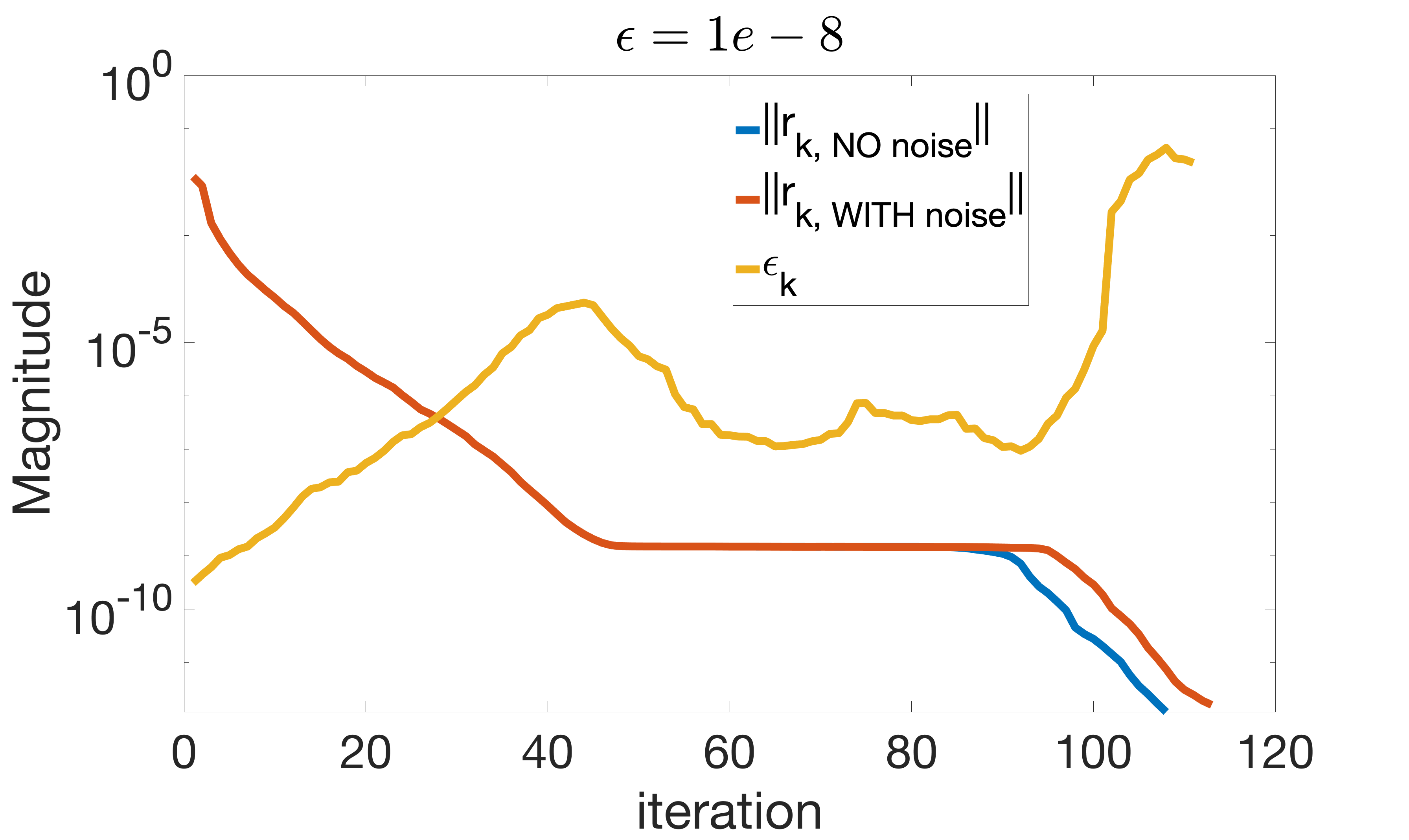
(a)

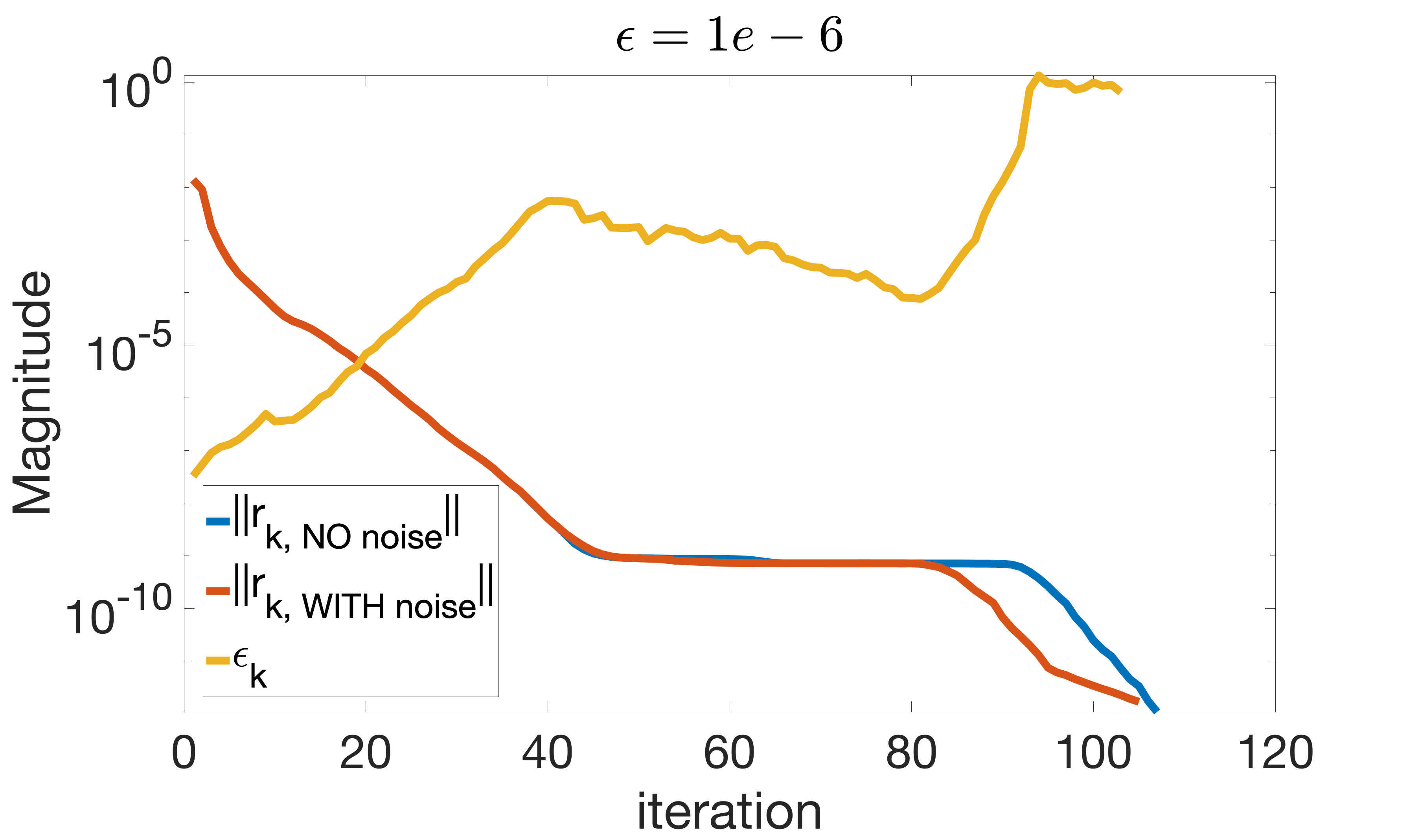
(b)

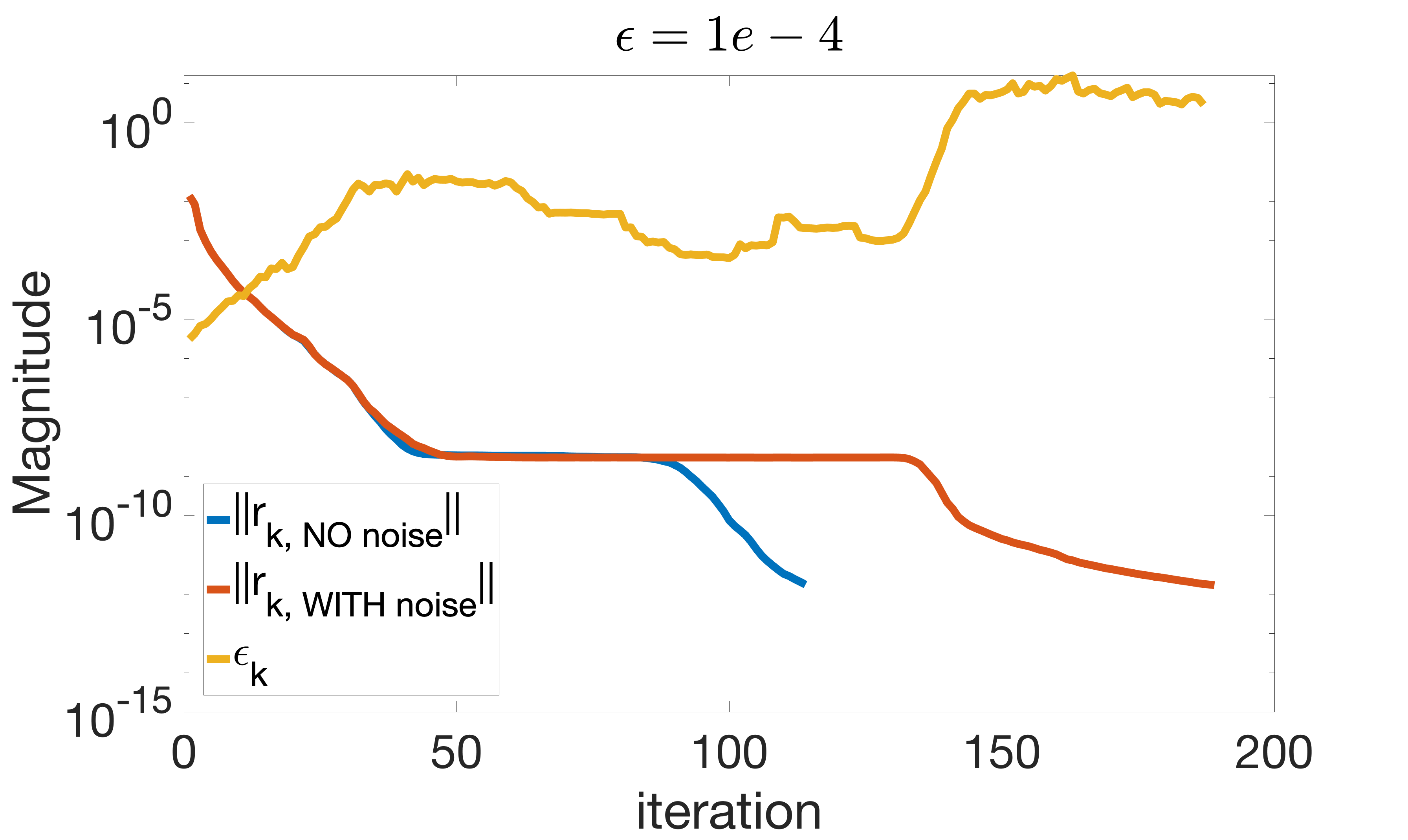
(c)

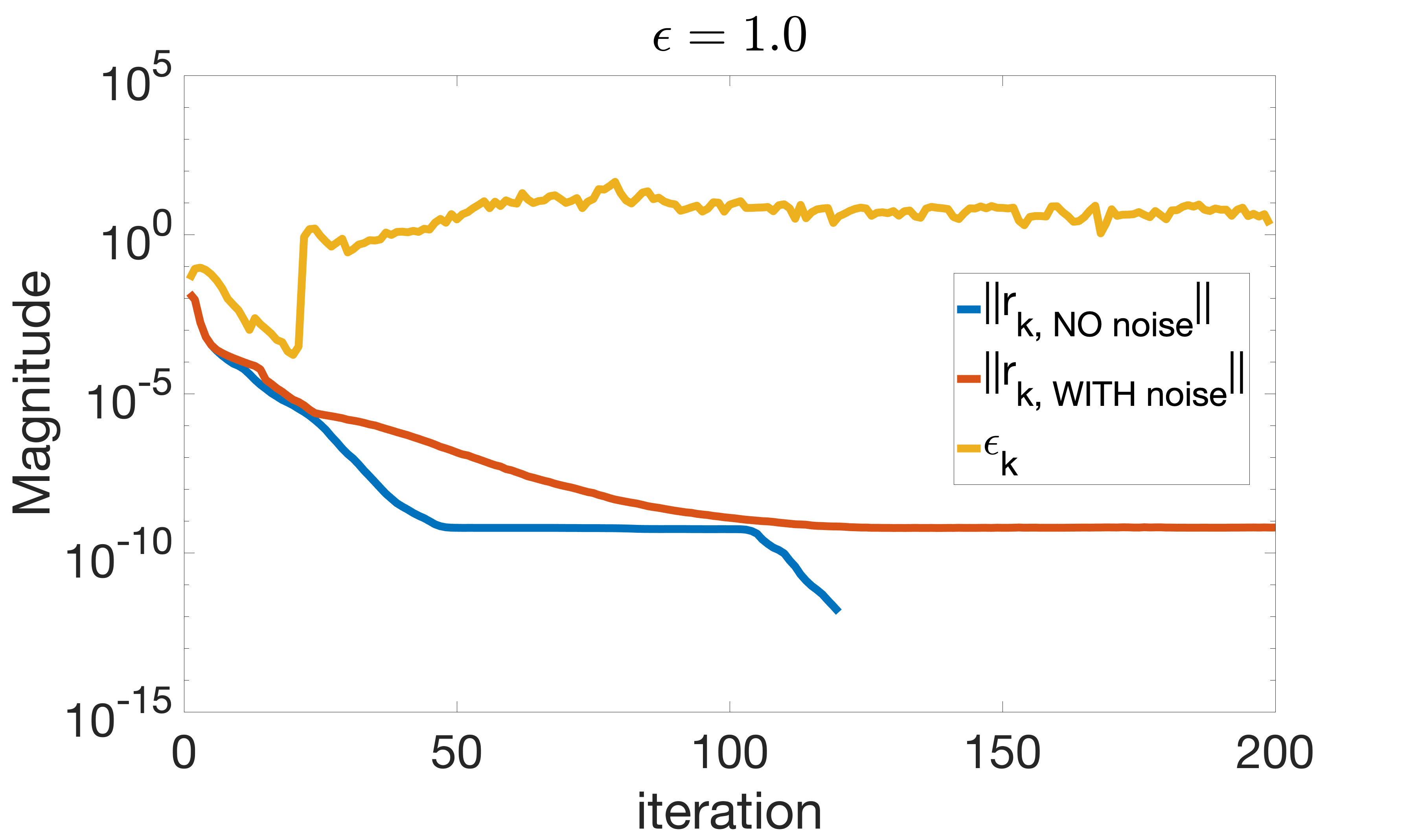
(d)

Figure 1: Approximate AA convergence history.

5.1.2 Reduced Alternating AA to solve sparse linear systems

We now use Reduced AAR to solve a set of linear systems where the matrices are open source and pulled from the SuiteSparse Matrix Collection (formerly known as the University of Florida Sparse Matrix Collection) [14], the Matrix Market Collection [6]. In Table 1, we report the matrices and their most significant properties. The sources used to retrieve the matrices are specified in Table 1 as well. The notation MM is used to refer to the Matrix Market Collection, and SS for the SuiteSparse Matrix Collection.

Matrix	Type	Size	Structure	Pos. def.	Source
fidap029	real	2,870	nonsymmetric	yes	MM
raefsky5	real	6,316	nonsymmetric	yes	SS
bcsstk29*	real	13,992	symmetric	no	SS
sherman3*	real	5,005	nonsymmetric	no	MM
sherman5*	real	3,312	nonsymmetric	no	MM
fidap008*	real	3,096	nonsymmetric	no	MM
chipcool0	real	20,082	nonsymmetric	no	SS
e20r0000*	real	4,241	nonsymmetric	no	MM
spmsrtls	real	29,995	nonsymmetric	no	SS
garon1*	real	3,175	nonsymmetric	no	SS
garon2*	real	13,535	nonsymmetric	no	SS
memplus	real	17,758	nonsymmetric	no	SS
saylr4	real	3,564	nonsymmetric	no	MM
xenon1*	real	48,600	nonsymmetric	no	SS
xenon2*	real	157,464	nonsymmetric	no	SS
venkat01	real	62,424	nonsymmetric	no	SS
QC2534	complex	2,534	non-Hermitian	no	SS
mplate*	complex	5,962	non-Hermitian	no	SS
light_in_tissue	complex	29,282	non-Hermitian	no	SS
kim1	complex	38,415	non-Hermitian	no	SS
chevron2	complex	90,249	non-Hermitian	no	SS

Table 1: List of matrices used for numerical experiments performed in Matlab.

The experiments compare the performance of GMRES with restart parameter equal to 50, Alternating AA, Subselected Alternating AA and Randomized Alternating AA. For each problem, two preconditioning techniques are used: Zero Fill-In Incomplete LU Factorization (ILU(0) for short) and Incomplete LU Factorization with Threshold (ILUT($\tau$) for short) [11]. When ILUT($\tau$) is used, the tolerance $\tau$ controls the level of sparsity in the incomplete LU factors. We set $\tau=10^{-4}$ and any zeros on the diagonal of the upper triangular factor are replaced by the local tolerance. The ILUT($\tau$) preconditioner is computed with a column pivoting and the pivot is chosen as the maximum magnitude entry in the column. For more details about ILU(0) and ILUT($\tau$) we refer to [4], [38, pp. 287–307]. A symmetric reverse Cuthill-McKee reordering [13] has been applied to some matrices to allow a stable construction of the ILU factors. The matrices that needed a reordering for the ILU preconditioner are marked with an asterisk close to their name in Table 1. Since the matrices xenon1 and xenon2 were poorly scaled, the ILU factors have been computed for these matrices only after a diagonal scaling. The diagonal scaling has been applied via a diagonal preconditioner on these matrices. Those situations where the matrices had zeros on the main diagonal were treated by setting to one the associated entries in the diagonal preconditioner. The Richardson relaxation parameter is set to $\omega=0.2$. The number of Richardson iterations between two Anderson updates for the AAR is $p=3$ and the history length is $m=20$. The least-squares problems related to Anderson mixing steps are solved via QR factorization with column pivoting of the rectangular matrix to the LHS. The RHS of the linear systems is obtained by multiplying the solution vector by the coefficient matrix $A$. The variation across single runs never exceeded $10\%$ in terms of computational time. A threshold of $10^{-8}$ is used as a stopping criterion on the relative residual $\ell^{2}$-norm. The heuristic proposed in Corollary 3.10 is used to automatically tune the dimensionality of the projection subspace at each AA step. To avoid introducing excessive computational overhead in fine tuning the dimensionality of the subspace, we add rows in batches, with each batch being 10% of the total number of rows in the original least-squares problem.

The performance of the linear solvers is evaluated through performance profiles [16]. Let us refer to $\mathcal{S}$ as the set of solvers and $\mathcal{P}$ as the test set. We assume that we have $n_{s}$ solvers and $n_{p}$ problems. In this paper, performance profiles are used to compare the computational times. To this end we introduce

$$t_{p,s}=\text{computing time to solve problem}\;p\;\text{with solver}\;s.$$

The comparison between the times taken by each solver is based on the performance ratio defined as

$$r_{p,s}=\frac{t_{p,s}}{\min\{t_{p,s}:s\in\mathcal{S}\}}.$$

The performance ratio allows one to compare the performance of solver $s$ on problem $p$ with the best performance by any solver to address the same problem $p$. In case a specific solver $s$ does not succeed in solving problem $p$, then a convention is adopted to set $r_{p,s}=r_{M}$ where $r_{M}$ is a maximal value. In our case we set $r_{m}=10,000$. The performance of one solver compared to the others’ on the whole benchmark set is displayed by the cumulative distribution function $\rho_{s}(\tau)$ that is defined as follows:

$$\rho_{s}(\tau)=\frac{1}{n_{p}}\text{size}\{p\in\mathcal{P}:r_{p,s}\leq\tau\}.$$

The value $\rho_{s}(\tau)$ represents the probability that solvers $s\in\mathcal{S}$ has a performance ratio $r_{p,s}$ less than or equal to the best possible ratio up to a scaling factor $\tau$. The convention adopted that prescribes $r_{p,s}=r_{M}$ if solver $s$ does not solve problem $p$ leads to the reasonable assumption that

$$r_{p,s}\in[1,r_{M}].$$

Therefore, $\rho_{s}(r_{M})=1$ and

$$\rho_{s}^{*}=\lim_{\tau\rightarrow r_{M}^{-}}\rho_{s}(\tau)$$

represents the probability that solver $s$ succeed in solving a generic problem from set $\mathcal{P}$. To improve the clarity of the graphs, we replace $\rho_{s}(\tau)$ with

$$\tau\mapsto\frac{1}{n_{p}}\text{size}\{p\in\mathcal{P}:\log_{2}(r_{p,s})\leq\tau\}$$

and we use this quantity for each performance profile displayed.

The numerical results with ILU(0) and ILUT($\tau$) are shown in Figures 2a and 2b, respectively. Randomized Alternating AA outperforms Subselected Alternating AA by converging on a larger set of problems, and outperforms standard AA and GMRES for time-to-solution. Therefore, an adaptive reduction of the dimensionality of the least-squares problem is shown to effectively reduce the total computational cost of AAR to iteratively solve a number of different sparse linear systems while still maintaining convergence.

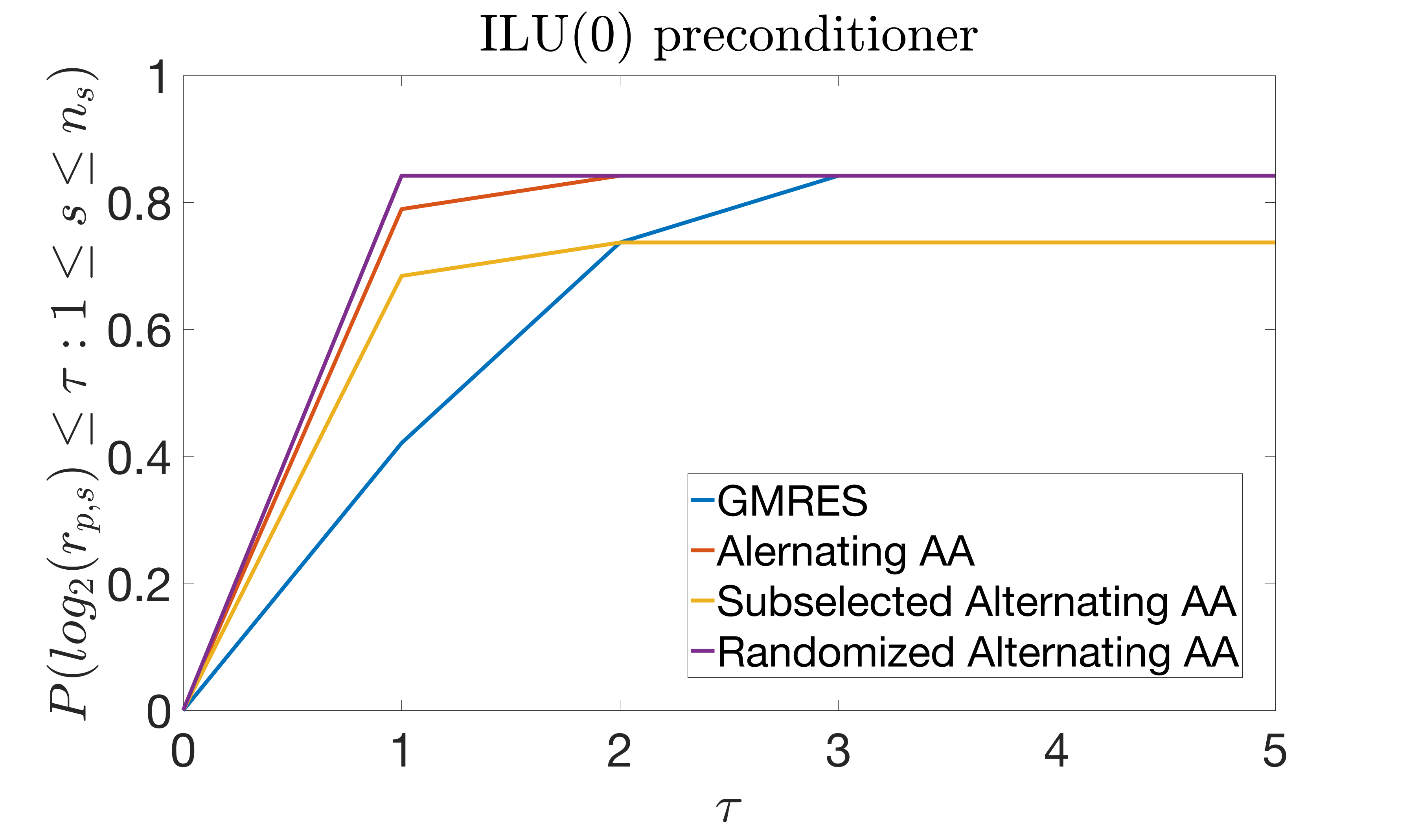
(a)

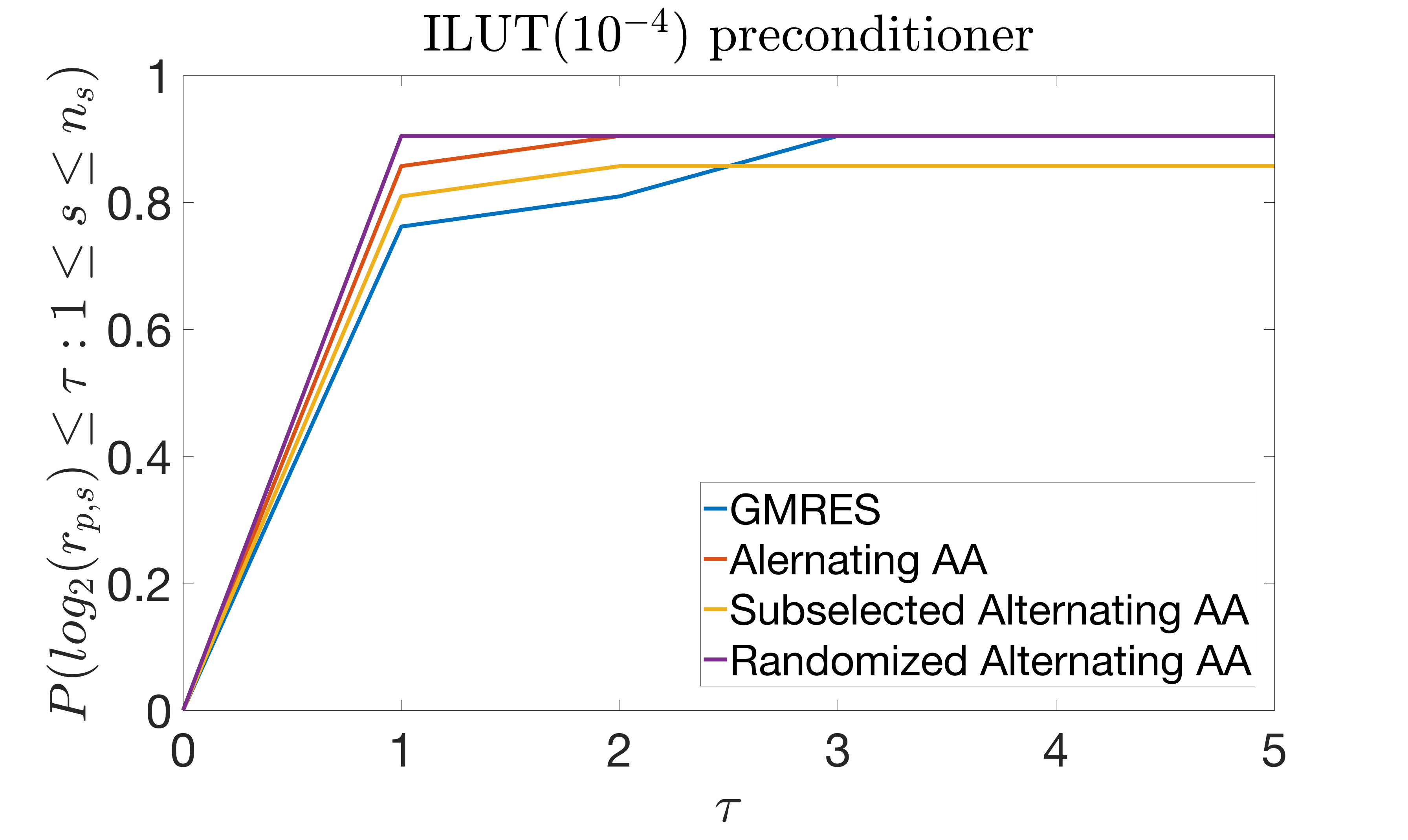
(b)

Figure 2: Performance profiles in a $\log_{2}$ scale.

5.2 Non-linear deterministic fixed-point iteration: Picard iteration for non-linear time-dependent Boltzmann equation

To illustrate the performance of Alternating AA with projected least-squares on deterministic non-linear problems, we chose the non-linear systems that arise from implicit time discretization of the non-relativistic Boltzmann equation, which is a widely used model for neutrino transport in nuclear astrophysics applications [30]. The non-relativistic Boltzmann equation is given by

(54) $$\partial_{t}{f}+\mathcal{T}(f)=\mathcal{C}(f)\>,$$

where $f(\boldsymbol{x},\omega,\epsilon,t)$ denotes the neutrino distribution function that describes the density of neutrino particles at position $\boldsymbol{x}\in\mathbb{R}^{3}$ traveling along direction $\omega\in\mathbb{S}^{2}$ with energy $\epsilon\in\mathbb{R}^{+}$ at time $t\in\mathbb{R}^{+}$. Here the advection and collision operators are denoted by $\mathcal{T}$ and $\mathcal{C}$, respectively. Implicit-explicit (IMEX) time integration schemes [32] are often used to solve (54), in which the collision term is treated implicitly to relax the excessive explicit time-step restriction, while an explicit advection term is used to avoid spatially coupled non-linear systems. With a simple backward Euler method, the implicit stage of an IMEX scheme applied to (54) at time $t^{n}$ takes the form

(55) $$f(\boldsymbol{x},\omega,\epsilon,t^{n+1})=f(\boldsymbol{x},\omega,\epsilon,t^{n})+\Delta t\,\mathcal{C}(f(\boldsymbol{x},\cdot,\cdot,t^{n+1}))\>,\quad\forall\boldsymbol{x}\in\mathbb{R}^{3}\>,$$

where we follow the approach in [26] and write the (space-time homogeneous) neutrino collision operator $\mathcal{C}$ as

(56) $$\mathcal{C}(f)={\eta_{\mbox{\tiny{Tot}}}}(f)-{\chi_{\mbox{\tiny{Tot}}}}(f)\,f\>,$$

where ${\eta_{\mbox{\tiny{Tot}}}}$ denotes the total emissivity and ${\chi_{\mbox{\tiny{Tot}}}}$ denotes the total opacity. As in [26], we formulate (55) at each time step into a non-linear fixed-point problem

(57) $$f^{n+1}=G(f^{n+1})\,\text{ with }\,G(f^{n+1}):=({f^{n}+\Delta t\eta_{\mbox{\tiny{Tot}}}(f^{n+1})})/({1+\Delta t\chi_{\mbox{\tiny{Tot}}}(f^{n+1})})\>.$$

This formulation ensures that the fixed-point operator $G$ is a contraction and allows for the standard Picard iteration as well as variants of AA to solve (55).

In the numerical tests, we solve the spatially-homogeneous implicit system (57) at one time step, in which we apply a discrete ordinate angular discretization with a 110-point Lebedev quadrature rule on $\mathbb{S}^{2}$ and 64 geometrically progressing energy nodes in $[0,300]$ (MeV). Here we compare the performance of five iterative solvers: Picard iteration, standard AA, Alternating AA, and two versions of Reduced Alternating AA – Subselected Alternating AA and Randomized Alternating AA. The history length $m=3$ is used for all four AA variants, and the alternating ones perform Anderson mixing every $p=3$ iterations. The Subselected Alternating AA and Randomized Alternating AA solvers are implemented as presented in Section 4 with the reduced dimension $s$ chosen to satisfy the bound (41), where $\epsilon=10^{-8}$ is used. Each solver is tested on problems at six different matter density values. In general, higher matter densities correspond to stronger collision effects, which make the implicit system more stiff and require more iterations to converge. In the test, the total emissivity and opacity are computed using opacity kernels provided in [10].

Figure 3 reports the iteration count and computation time required for each compared solver at various matter densities. These reported results are averaged over 30 runs. Figure 3a confirms that AA and Alternating AA require significantly fewer iterations to reach the prescribed $10^{-10}$ relative tolerance than the Picard iteration, especially for problems at higher densities (more stiff). Randomized Alternating AA essentially resembles the iteration counts of Alternating AA, while the Subselected Alternating AA requires much higher iteration counts than other AA variants. Figure 3b illustrates that AA actually takes more computation time than Picard iteration, which indicates that the additional cost of solving least-squares problems outweighs the reduction of iteration counts. Alternating AA lowers the computation time of AA by reducing the frequency of solving the least-squares problems, and Randomized Alternating AA further improves the computation time by approximating the least-squares solution with solution to a sparsely projected smaller problem.

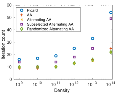
(a)

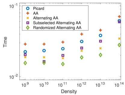
(b)

Figure 3: Iteration counts and computation time (in $\log$ scale) for various fixed-point solvers for solving the non-linear system (57) at different matter density, which corresponds to the stiffness of the system.

6 Conclusion and future development

Although AA has been shown to significantly improve the convergence of fixed-point iterations in several scientific applications, effectively performing AA for large scale problems without introducing excessive computational burden remains still a challenge. One possibility to reduce the computational cost consists in projecting the least-squares to compute the Anderson mixing onto a projection subspace, but this may compromise the convergence of the scheme.

We derived rigorous theoretical bounds for AA that allow for efficient approximate calculations of the residual, which reduce computational time and memory storage while maintaining convergence. The theoretical bounds provide useful insight to judiciously inject inaccuracy in the calculations whenever this allows to alleviate the computational burden without compromising the final accuracy of the physics based solver. In particular, we consider situations where the inaccuracy arises from projecting the least-squares problem onto a subspace.

Guided by the theoretical bounds, we constructed a heuristic that dynamically adjusts the dimension of the projection subspace at each iteration. As the process approaches convergence, the backward error decreases, which allows for an increase of the inaccuracy of the least-squares calculations while still maintaining the residual norm within the prescribed bound. This reduces the need for very accurate calculations needed to converge. While previous theoretical results provide error estimates when the accuracy is fixed a priori throughout the fixed-point scheme, thus potentially compromising the final attainable accuracy, our study allows for adaptive adjustments of the accuracy to perform AA while still ensuring that the final residual norm drops below a prescribed threshold. The resulting numerical scheme, called Reduced Alternating AA, is clearly preferable over standard Alternating AA when the computational budget is limited.

Numerical results on linear systems and non-linear non-relativistic Boltzmann equation show that our heuristic can be used to effectively reduce the computational time of Reduced Alternating AA without affecting the final attainable accuracy compared to traditional methods to apply AA.

Future work will be dedicated to apply Reduced Alternating AA to non-linear stochastic fixed point iterations arising from: (i) Monte Carlo methods for solving the Boltzmann equation and (ii) training of physics informed graph convolutional neural networks for the prediction of materials properties from atomic information.

References

- [1] K. Aghazade, A. Gholami, H. S. Aghamiry, and S. Operto, Anderson-accelerated augmented Lagrangian for extended waveform inversion, Geophysics, 87 (2022), p. R79, https://doi.org/dx.doi.org/10.1190/geo2021-0409.1, http://dx.doi.org/10.1190/geo2021-0409.1, https://arxiv.org/abs/http://dx.doi.org/10.1190/geo2021-0409.1.
- [2] D. G. Anderson, Iterative procedures for nonlinear integral equations, Journal of the Association for Computing Machinery, 12 (1965).
- [3] A. S. Banerjee, P. Suryanarayana, and J. E. Pask, Periodic Pulay method for robust and efficient convergence acceleration of self-consistent field iterations, Chemical Physics Letters, 647 (2016), pp. 31–35, https://doi.org/10.1016/j.cplett.2016.01.033, https://linkinghub.elsevier.com/retrieve/pii/S0009261416000464 (accessed 2021-04-06).
- [4] M. Benzi, Preconditioning techniques for large linear systems: a survey, Journal of Computational Physics, 182 (2002), pp. 418–477.
- [5] W. Bian, X. Chen, and C. T. Kelley, Anderson acceleration for a class of nonsmooth fixed-point problems, SIAM Journal on Scientific Computing, 43 (2021), pp. S1–S20, https://doi.org/10.1137/20M132938X, https://doi.org/10.1137/20M132938X, https://arxiv.org/abs/https://doi.org/10.1137/20M132938X.
- [6] R. F. Boisvert, R. Pozo, K. Remington, R. F. Barrett, and J. J. Dongarra, Matrix Market: a web resource for test matrix collections, Springer US, Boston, MA, 1997, pp. 125–137, https://doi.org/10.1007/978-1-5041-2940-4_9, https://doi.org/10.1007/978-1-5041-2940-4_9.
- [7] C. Brezinski, S. Cipolla, M. Redivo-Zaglia, and Y. Saad, Shanks and Anderson-type acceleration techniques for systems of nonlinear equations, IMA Journal of Numerical Analysis, (2021), https://doi.org/10.1093/imanum/drab061, https://doi.org/10.1093/imanum/drab061, https://arxiv.org/abs/https://academic.oup.com/imajna/advance-article-pdf/doi/10.1093/imanum/drab061/39919343/drab061.pdf. drab061.
- [8] C. Brezinski, S. Cipolla, M. Redivo-Zaglia, and Y. Saad, Shanks and Anderson-type acceleration techniques for systems of nonlinear equations, IMA Journal of Numerical Analysis, (2021), https://doi.org/10.1093/imanum/drab061, https://doi.org/10.1093/imanum/drab061, https://arxiv.org/abs/https://academic.oup.com/imajna/advance-article-pdf/doi/10.1093/imanum/drab061/39919343/drab061.pdf.
- [9] C. Brezinski, M. Redivo-Zaglia, and Y. Saad, Shanks sequence transformations and Anderson acceleration, SIAM Review, 60 (2018), pp. 646–669, https://doi.org/10.1137/17M1120725, https://epubs.siam.org/doi/10.1137/17M1120725 (accessed 2021-04-06).
- [10] S. W. Bruenn, Stellar core collapse - Numerical model and infall epoch, Astrophysical Journal Supplement Series, 58 (1985), pp. 771–841.
- [11] T. F. Chan and H. A. Van der Vorst, Approximate and Incomplete Factorizations, Parallel Numerical Algorithms, Springer Netherlands, Dordrecht, 1997, pp. 167–202, https://doi.org/10.1007/978-94-011-5412-3_6, https://doi.org/10.1007/978-94-011-5412-3_6.
- [12] K. Chen and C. Vuik, Non-stationary Anderson acceleration with optimized damping, ArXiv:2202.05295, 2022, https://doi.org/10.48550/ARXIV.2202.05295, https://arxiv.org/abs/2202.05295.
- [13] E. Cuthill and J. McKee, Reducing the bandwidth of sparse symmetric matrices, in ACM ’69 Proceeding of the national conference, New York, NY, United States, 1969, pp. 157–172, https://doi.org/10.1109/CCGRID.2019.00092.
- [14] T. A. Davis and Y. Hu., The SuiteSparse Matrix Collection (formerly known as the University of Florida Sparse Matrix Collection), 2011, https://doi.org/https://doi.org/10.1145/2049662.2049663, http://www.cise.ufl.edu/research/sparse/matrices/.
- [15] V. P. DeCaria, C. D. Hauck, and M. T. P. Laiu, Analysis of a new implicit solver for a semiconductor model, SIAM Journal on Scientific Computing, 43 (2021), pp. B733–B758, https://doi.org/10.1137/20M1365922, https://doi.org/10.1137/20M1365922, https://arxiv.org/abs/https://doi.org/10.1137/20M1365922.
- [16] E. D. Dolan and J. Moré, Benchmarking optimization software with performance profiles, Mathematical Programming, 91 (2002), pp. 201–212.
- [17] C. Evans, S. Pollock, L. G. Rebholz, and M. Xiao, A proof that Anderson acceleration improves the convergence rate in linearly converging fixed-point methods (but not in those converging quadratically), SIAM Journal on Numerical Analysis, 58 (2020), pp. 788–810, https://doi.org/10.1137/19M1245384, https://doi.org/10.1137/19M1245384, https://arxiv.org/abs/https://doi.org/10.1137/19M1245384.
- [18] H. Fang and Y. Saad, Two classes of multisecant methods for nonlinear acceleration, Numerical Linear Algebra with Applications, 16 (2009), pp. 197–221.
- [19] H. Fang and Y. Saad, Two classes of multisecant methods for nonlinear acceleration, Numerical Linear Algebra with Applications, 16 (2009), pp. 197–221, https://doi.org/10.1002/nla.617, http://doi.wiley.com/10.1002/nla.617 (accessed 2021-04-06).
- [20] A. Fu, J. Zhang, and S. Boyd, Anderson accelerated Douglas–Rachford splitting, SIAM Journal on Scientific Computing, 42 (2020), pp. A3560–A3583, https://doi.org/10.1137/19M1290097, https://doi.org/10.1137/19M1290097, https://arxiv.org/abs/https://doi.org/10.1137/19M1290097.
- [21] G. Golub, Numerical methods for solving linear least squares problems, Numerische Mathematik, 7 (1965), pp. 206–216, https://doi.org/https://doi.org/10.1007/BF01436075.
- [22] G. H. Golub and R. S. Varga, Chebyshev semi-iterative methods, successive over-relaxation iterative methods, and second-order Richardson iterative methods, parts I and II, Numerische Mathematik, 3 (1961), pp. 147–156, 157–168.
- [23] J. F. Grcar, M. A. Saunders, and Z. Su, Estimates of optimal backward perturbations for linear least squares problems, Technical Report SOL 2007-1. Department of Management Science and Engineering, Stanford University, Stanford, CA, 2007.
- [24] E. Hallman and M. Gu, LSMB: Minimizing the backward error for least-squares problems, SIAM Journal on Matrix Analysis and Applications, 39 (2018), pp. 1295–1317, https://doi.org/10.1137/17M1157106, https://doi.org/10.1137/17M1157106, https://arxiv.org/abs/https://doi.org/10.1137/17M1157106.
- [25] M. P. Laiu, Z. Chen, and C. D. Hauck, A fast implicit solver for semiconductor models in one space dimension, Journal of Computational Physics, 417 (2020), p. 109567, https://doi.org/https://doi.org/10.1016/j.jcp.2020.109567, https://www.sciencedirect.com/science/article/pii/S0021999120303417.
- [26] M. P. Laiu, E. Endeve, R. Chu, J. A. Harris, and O. E. B. Messer, A DG-IMEX method for two-moment neutrino transport: Nonlinear solvers for neutrino–matter coupling, The Astrophysical Journal Supplement Series, 253 (2021), p. 52, https://doi.org/10.3847/1538-4365/abe2a8, https://doi.org/10.3847/1538-4365/abe2a8.
- [27] M. P. Laiu, J. A. Harris, R. Chu, and E. Endeve, Thornado-transport: Anderson- and GPU-accelerated nonlinear solvers for neutrino-matter coupling, Journal of Physics: Conference Series, 1623 (2020), p. 012013, https://doi.org/10.1088/1742-6596/1623/1/012013, https://doi.org/10.1088/1742-6596/1623/1/012013.
- [28] M. Lupo Pasini, Convergence analysis of Anderson-type acceleration of Richardson’s iteration, Numerical Linear Algebra with Applications, 26 (2019), p. e2241, https://doi.org/10.1002/nla.2241, https://onlinelibrary.wiley.com/doi/abs/10.1002/nla.2241 (accessed 2021-04-06).
- [29] V. V. Mai and M. Johansson, Nonlinear acceleration of constrained optimization algorithms, in ICASSP 2019 - 2019 IEEE International Conference on Acoustics, Speech and Signal Processing (ICASSP), 2019, pp. 4903–4907, https://doi.org/10.1109/ICASSP.2019.8682962.
- [30] A. Mezzacappa and O. Messer, Neutrino transport in core collapse supernovae, Journal of Computational and Applied Mathematics, 109 (1999), pp. 281–319, https://doi.org/https://doi.org/10.1016/S0377-0427(99)00162-4, https://www.sciencedirect.com/science/article/pii/S0377042799001624.
- [31] W. Ouyang, Y. Peng, Y. Yao, J. Zhang, and B. Deng, Anderson acceleration for nonconvex ADMM based on Douglas-Rachford splitting, Optimization, 39 (2020), pp. 221–239, https://doi.org/doi.org/10.1111/cgf.14081, https://doi.org/10.1111/cgf.14081, https://arxiv.org/abs/https://doi.org/10.1111/cgf.14081.
- [32] L. Pareschi and G. Russo, Implicit-Explicit Runge-Kutta Schemes and Application to Hyperbolic Systems with Relaxation, Journal of Scientific Computing, 25 (2005), pp. 129–155.
- [33] S. Pollock and L. G. Rebholz, Anderson acceleration for contractive and noncontractive operators, IMA Journal of Numerical Analysis, 41 (2021), pp. 2841–2872, https://doi.org/10.1093/imanum/draa095, https://doi.org/10.1093/imanum/draa095, https://arxiv.org/abs/https://academic.oup.com/imajna/article-pdf/41/4/2841/40757730/draa095.pdf.
- [34] F. A. Potra and H. Engler, A characterization of the behavior of the Anderson acceleration on linear problems, Linear Algebra and its Applications, 438 (2013), pp. 1002–1011, https://doi.org/10.1016/j.laa.2012.09.008, https://linkinghub.elsevier.com/retrieve/pii/S0024379512006738 (accessed 2021-04-06).
- [35] F. A. Potra and H. Engler, A characterization of the behavior of the Anderson acceleration on linear problems, Linear Algebra and its Applications, 438 (2013), pp. 1002–1011.
- [36] P. P. Pratapa, P. Suryanarayana, and J. E. Pask, Anderson acceleration of the jacobi iterative method: an efficient alternative to krylov methods for large, sparse linear systems, Journal of Computational Physics, 306 (2016), pp. 43–54.
- [37] Y. Saad, Iterative Methods for Sparse Linear Systems, SIAM, (2003), https://doi.org/10.2113/gsjfr.6.1.30, http://www.stanford.edu/class/cme324/saad.pdf, https://arxiv.org/abs/0806.3802.
- [38] Y. Saad, Iterative Methods for Sparse Linear Systems (Second Edition), Society for Industrial and Applied Mathematics (SIAM), Philadelphia, 2003.
- [39] Y. Saad and M. H. Schultz, GMRES: A generalized minimal residual algorithm for solving nonsymmetric linear systems, SIAM Journal on Scientific and Statistical Computing, 7 (1986), pp. 856–869.
- [40] V. Simoncini and D. Szyld, Theory of approximate krylov subspace methods and applications to scientific computing, SIAM Journal on Scientific Computing, 25 (2003), pp. 454–477.
- [41] P. Suryanarayana, P. P. Pratapa, and J. E. Pask, Alternating Anderson-Richardson method: an efficient alternative to preconditioned Krylov methods for large, sparse linear systems, Computer Physics Communications, 234 (2019), pp. 278–285, https://doi.org/10.1016/j.cpc.2018.07.007, https://linkinghub.elsevier.com/retrieve/pii/S001046551830256X (accessed 2021-04-06).
- [42] A. Toth, J. A. Ellis, T. Evans, S. Hamilton, C. T. Kelley, R. Pawlowski, and S. Slattery, Local improvement results for Anderson acceleration with inaccurate function evaluations, SIAM Journal on Scientific Computing, 39 (2017), pp. S47–S65, https://doi.org/10.1137/16M1080677, https://epubs.siam.org/doi/10.1137/16M1080677 (accessed 2021-04-06).
- [43] A. Toth and C. T. Kelley, Convergence analysis for Anderson acceleration, SIAM Journal on Numerical Analysis, 53 (2015), pp. 805–819, https://doi.org/10.1137/130919398, http://epubs.siam.org/doi/10.1137/130919398 (accessed 2021-04-06).
- [44] H. F. Walker and P. Ni, Anderson acceleration for fixed-point iteration, SIAM Journal on Numerical Analysis, 49 (2011), pp. 1715–17359.
- [45] H. F. Walker and P. Ni, Anderson Acceleration for fixed-point iterations, SIAM Journal on Numerical Analysis, 49 (2011), pp. 1715–1735, https://doi.org/10.1137/10078356X, http://epubs.siam.org/doi/10.1137/10078356X (accessed 2021-04-06).
- [46] J. Zhang, B. O’Donoghue, and S. Boyd, Globally convergent type-I Anderson acceleration for nonsmooth fixed-point iterations, SIAM Journal on Optimization, 30 (2020), pp. 3170–3197, https://doi.org/10.1137/18M1232772, https://doi.org/10.1137/18M1232772, https://arxiv.org/abs/https://doi.org/10.1137/18M1232772.