Channel Estimation with Hybrid Reconfigurable Intelligent Metasurfaces

Abstract

Reconfigurable Intelligent Surfaces are envisioned to play a key role in future wireless communications, enabling programmable radio propagation environments. They are usually considered as almost passive planar structures that operate as adjustable reflectors, giving rise to a multitude of implementation challenges, including the inherent difficulty in estimating the underlying wireless channels. In this paper, we focus on the recently conceived concept of Hybrid Reconfigurable Intelligent Surfaces, which do not solely reflect the impinging waveform in a controllable fashion, but are also capable of sensing and processing an adjustable portion of it. We first present implementation details for this metasurface architecture and propose a convenient mathematical model for characterizing its dual operation. As an indicative application of HRISs in wireless communications, we formulate the individual channel estimation problem for the uplink of a multi-user HRIS-empowered communication system. Considering first a noise-free setting, we theoretically quantify the advantage of HRISs in notably reducing the amount of pilots needed for channel estimation, as compared to the case of purely reflective RISs. We then present closed-form expressions for the Mean-Squared Error (MSE) performance in estimating the individual channels at the HRISs and the base station for the noisy model. Based on these derivations, we propose an automatic differentiation-based first-order optimization approach to efficiently determine the HRIS phase and power splitting configurations for minimizing the weighted sum-MSE performance. Our numerical evaluations demonstrate that HRISs do not only enable the estimation of the individual channels in HRIS-empowered communication systems, but also improve the ability to recover the cascaded channel, as compared to existing methods using passive and reflective RISs.

I Introduction

RISs are an emerging technology for the future $6$-th Generation (6G) of wireless communications, enabling dynamically programmable signal propagation over the wireless medium [2, 3, 4, 5]. RISs are planar structures comprised typically of multiple metamaterial elements, whose ElectroMagnetic (EM) properties can be externally controlled in a nearly passive manner, allowing them to realize various reflection and scattering profiles [6]. By properly adjusting the reflection properties of the metamaterial elements, RISs can constructively strengthen/destructively weaken the desired/undesired signals at the target receiver(s). This ability of RISs has been exploited in various promising communication systems, such as multi-user Multiple-Input Multiple-Outputs communications [7, 8], simultaneous wireless information and power transfer systems [9, 10], and physical-layer security [11], for improving the respective performance. Achieving those performance gains with RISs often relies on accurate Channel State Information (CSI). However, their passive nature implies that they can only act as adjustable reflectors, and thus, neither receive nor transmit their own data. This renders channel estimation a significant, but challenging task for RIS-based systems [12].

In RIS-aided uplink communications, a signal transmitted from each User Terminal (UT) to the Base Station (BS) undergoes at least two channels, namely, the UTs-RIS and RIS-BS channels. With RISs being passive without any signal processing capability, the common approach to acquire CSI is to estimate only the entangled combined effect of the latter channels, i.e., the cascaded channel [13, 14, 15] at the BS. This can be achieved by having the UTs send known pilot symbols, which are reflected by the RIS such that the channel outputs at the BS are used to estimate the overall channel. This approach has, however, two main drawbacks. First, since the number of reflective elements of RISs is usually very large, the cascaded channel is comprised of many unknown parameters that need to be estimated, which requires large pilot periods, and thus, significantly reduces the spectrum utilization efficiency. For example, for a system with $K$ UTs, $N$ RIS meta-atom elements, and $M$ BS antennas, the cascaded channel consists of $KNM$ coefficients. To alleviate this drawback, several methods have been proposed to reduce the pilots, which impose a model on the overall channel having less coefficients, via, e.g., grouping the RIS elements [16], exploiting the presence of a common channel [17], and imposing a sparsity prior [18]. The second drawback of passive RISs is that one can only estimate the cascaded channel, instead of the individual ones, which limits the plasticity for the transmission scheme design and restricts the network management flexibility [19]. As discussed in [20], the individual UTs-RIS and RIS-BS channels are needed for some precoding designs. In addition, there exist certain scenarios where the RIS-BS channel may vary less rapidly than the UTs-RIS combined one. For those cases, only the UTs-RIS channel needs to estimated frequently, thus, it is desirable to be capable of recovering the UTs-RIS and RIS-BS channels individually [12].

To overcome the aforementioned challenges with purely reflective RIS, it was recently proposed to equip RISs with minimal receive Radio-Frequency (RF) chains and antenna elements [21, 22, 23, 24]. In such architectures, some of the RIS elements are replaced with active receive antennas, which are connected via dedicated RF chains to a digital processor, and thus, have some signal processing capabilities such as reception and decoding. While such architectures enable the estimation of the individual UTs-RIS and RIS-BS channels, they involve placing additional receivers along the RIS, possibly reducing its number of reflective elements. In addition, they are incapable of estimating the exact channel, since the signals observed at the RIS reflective elements are not measured, but only those acquired at the receive antenna elements.

In parallel to the application of metasurfaces as passive reflective RISs, active metasurfaces have recently emerged as an appealing technology for realizing low-cost and low-power large-scale MIMO antennas [25]. Dynamic Metasurface Antennas pack large numbers of tunably radiative metamaterials on top of waveguides, resulting in MIMO transceivers with advanced analog processing capabilities [26, 27, 28, 29, 30]. While the implementation of DMAs differs from passive RISs, the similarity in the structure of the metamaterial elements between them indicates the feasibility of designing hybrid reflecting and sensing elements. This motivates studying the benefits from such a hybrid metasurface architecture, as an efficient means of facilitating RIS-empowered wireless communications, localization, and sensing.

In our previous overview article [31], we proposed the HRIS architecture, which is capable of simultaneously reflecting and receiving the incoming signal in an element-by-element controllable manner. HRISs differ from both conventional passive RISs, which are usually metasurfaces operating in almost energy neutral tunable reflection, as well as from active DMAs that operate similar to conventional transceiver antennas. In HRISs, each metamaterial element enables simultaneous adjustable reflection and reception of the impinging signals. This controllable hybrid operation of HRISs yields an architecture which generalizes RISs with interleaved reception and reflection meta-atoms, as in [21, 22, 23, 24]. More specifically, in [31], we overviewed the opportunities and challenges of the HRIS concept, highlighting a hardware design for its implementation and presenting a full-wave-simulation-based proof-of-concept. However, no technical analysis relevant to the exploitation of the signal processing capability at the HRIS side, and consequently of the availability of a portion of the received impinging signal, was provided. In this work, we fill this gap by considering HRIS-assisted multi-user MIMO communication systems and investigating the individual channel estimation problem. We show that the reception signal processing capability of HRISs allows the system to simultaneously estimate the individual channels, i.e., the UTs-HRIS channel at the HRIS side and the HRIS-BS at the BS, via reusing the same transmitted pilot symbols. We first theoretically quantify the advantages of the HRIS in terms of pilot reduction for the case without thermal noise. Then, considering the presence of this noise, we derive closed-form expressions for the MSEs of the estimation of the individual channels at the HRIS and BS, respectively. Based on these derivations, we provide a gradient-based optimization approach to efficiently configure the HRIS for minimizing the weighted sum-MSE, where the gradients of the complicated sum-MSE performance metric with respect to the HRIS tunable parameters are computed using Automatic Differentiation (AD).

The main contributions of this paper are summarized as follows:

• Hybrid Reflecting and Sensing RIS Architecture: We focus on the recently conceived concept of HRISs, which enables metasurfaces to reflect the impinging signal in an element-by-element controllable manner, while simultaneously sensing a portion of it. We specifically discuss the feasibility of hybrid meta-atom elements, present their high-level description, and provide a mathematical model for HRIS-empowered wireless systems in a manner that is amenable to system design.

• Estimation of the Individual Channels in HRIS-Aided Systems: We present an initial study on the potential gains of HRISs in multi-user MIMO communication systems, by considering the individual channels estimation problem. We first characterize the number of pilots needed to estimate the channels for the case without noise, and analytically demonstrate the gains of HRISs compared to pure reflective RISs. We then consider typical noisy settings and derive the MSE for the estimation of the UTs-HRIS channel at the HRIS and the HRIS-BS channel at the BS.

• AD-based Gradient Optimization for HRIS Configuration: Since the MSE depends on the configuration of the HRIS, we formulate a weighted sum-MSE minimization problem. The resulting problem is very challenging due to the complicated form of the objective and the large number of optimization variables. To deal with this, we propose a gradient-based solution to efficiently solve the problem. Inspired by the recent work [32], the gradients of the complicated sum-MSE objective function with respect to the HRIS parameters are computed analytically with AD. The effectiveness of the proposed algorithm is verified numerically.

• Numerical Evaluation: Our simulation results showcase the inherent trade-off of HRISs concerning their ability to estimate the individual channels. Furthermore, it is demonstrated that, even when one aims to solely estimate the cascaded channel, HRISs outperforms conventional (nearly) passive and reflective RISs [17] when the same pilot length is used.

The remainder of this paper is organized as follows. Section II presents the proposed model for generic HRIS operation as well as the proposed HRISs-assisted channel estimation approach. The individual channel estimation problem is investigated in Section III, which also includes the proposed gradient-based optimization for the HRISs phase and power splitting parameters. Numerical evaluations are presented in Section IV, and Section V provides concluding remarks.

Throughout the paper, we use boldface lower-case and upper-case letters for vectors and matrices, respectively, while calligraphic letters are used for sets. The vectorization operator, transpose, conjugation, Hermitian transpose, trace, and expectation are represented by ${\rm vec}(\cdot)$, $(\cdot)^{T}$, $(\cdot)^{{\dagger}}$, $(\cdot)^{H}$, ${\rm{Tr}}\left(\cdot\right)$, and $\mathds{E}\{\cdot\}$, respectively. The notation ${\rm blkdiag}\left\{{\bf A}_{1},{\bf A}_{2},\ldots,{\bf A}_{n}\right\}$ denotes a block diagonal matrix with diagonal blocks given by ${\bf A}_{1},{\bf A}_{2},\ldots,{\bf A}_{n}$, and $[\mathbf{A}]_{i,j}$ denotes the $(i,j)$-th element of $\mathbf{A}$. Finally, $\mathbb{C}$ is the set of complex numbers.

II HRISs and System Modeling

We first present a high-level description of the proposed hybrid metamaterial elements, followed by the considered system model for HRIS-empowered wireless communications. We then detail a simple, yet convenient, model for the HRIS operation and present the proposed approach for the estimation of the individual channels.

II-A Hybrid Metasurfaces

A rich body of literature has examined the fabrication of solely reflective RISs using metamaterials. A variety of implementations have been recently presented in [6, 33], ranging from RISs that change the wave propagation inside a multi-scattering environment for improving the received signal, to those which realize anomalous reflection, such that the reflected beam does not follow Snell’s law and is directed towards desired directions. More recently, RISs which simultaneously refract and relfect their impinging signals were proposed to offer $360^{\circ}$ coverage [34, 35, 36]. In all those efforts, the RIS is not designed to sense the impinging signal.

Metasurfaces can be designed to operate in a hybrid reflecting and sensing manner. Such hybrid operation requires that each metasurface element is capable of simultaneously reflecting a portion of the impinging signal and receiving another portion of it in a controllable manner. As illustrated in Fig. 1, a simple mechanism for implementing such an operation is to couple each element to a waveguide. The signals coupled to the waveguides are then measured by receive RF chains and used to infer the necessary information about the channel. A detailed description of the practical implementation of such hybrid metamaterials can be found in [37], where it was experimentally demonstrated that such surface configurations of hybrid metamaterials can be used to reflect in a reconfigurable manner, while using the sensed portion of the signal to locally recover its angle-of-arrival. In this paper, we are interested in examining the potential benefits of the HRIS paradigm in wireless communications. To this end, we present in the sequel a simple model capturing the simultaneous reflecting and sensing operation of HRISs, which is later on deployed to study HRIS-empowered wireless communications.

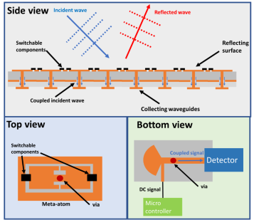
Figure 1: Illustration of a hybrid meta-atom which is capable of simultaneously reflecting a portion of its impinging wave in a reconfigurable manner, while feeding another portion of it to a receiving RF chain for baseband processing.

II-B HRIS Operation Modeling

To model the dual reflection-reception operation of HRISs, we consider a hybrid metasurface comprised of $N$ meta-atom elements, which are connected to a digital controller via $N_{r}$ reception RF chains. Let $r_{l}(n)$ denote the radiation observed by the $l$-th HRIS element ($l=1,2,\ldots,N$) at the $n$-th time instance. A portion of this signal, dictated by the parameter $\rho_{l}\left(n\right)\in[0,1]$, is reflected with a controllable phase shift $\psi_{l}\left(n\right)\in[0,2\pi)$, and thus the reflected signal from the $l$-th element at the $n$-th time instant can be mathematically expressed as:

$$y_{l}^{\rm RF}(n)=\rho_{l}\left(n\right)e^{\jmath\psi_{l}\left(n\right)}r_{l}(n).$$ (1)

The remainder of the observed signal is locally processed via analog combining and digital processing. The signal forwarded to the $r$-th RF chain via combining, with $r\in\{1,2,\ldots,N_{r}\}$, from the $l$-th element at the $n$-th time instant is consequently given by

$$y_{r,l}^{\rm RC}(n)=(1-\rho_{l}\left(n\right))e^{\jmath\phi_{r,l}\left(n\right)}r_{l}(n),$$ (2)

where $\phi_{r,l}\left(n\right)\in[0,2\pi)$ represents the adjustable phase that models the joint effect of the response of the $l$-th meta-atom and the subsequent analog phase shifting. The proposed HRIS operation model is illustrated in Fig. 2.

The operation of conventional passive and reflective RISs can be treated as a special case of the HRIS architecture, by setting all $\rho_{l}\left(n\right)$ in (1) equal to $1$. Compared with existing relay techniques, HRISs bring forth two major advantages. First, HRISs allow full-duplex operation (i.e., simultaneous reflection and reception) without inducing any self interference, which is unavoidable in full-duplex relaying systems. Second, HRISs require low power consumption since they do not need power amplifiers utilized by active transmit arrays; a typical receive RF consists of a low noise amplifier, a mixer which downconverts the signal from RF to baseband, and an analog-to-digital converter [38].

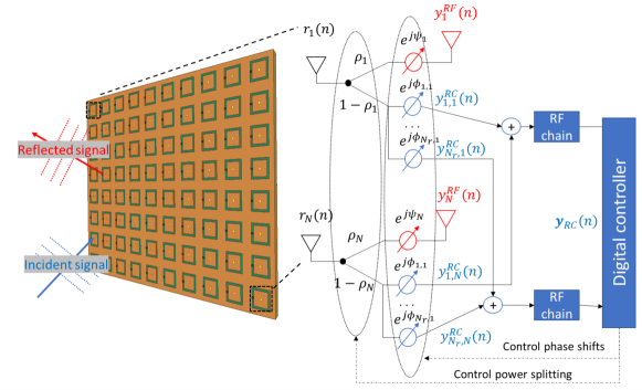
Figure 2: A simple model for the proposed HRIS operation. The parameter $\rho_{l}$ models the portion of the impinging signal at the $l$-th meta-atom of the HRIS that gets tunably reflected, while $\psi_{l}$ and $\phi_{r,l}$ model the meta-atom’s controllable phase shift and the joint effect of its response together with the analog phase shift before the $r$-th receive RF chain, respectively.

The resulting signal model at the HRIS can be expressed in vector form, as follows. By stacking the received signals $r_{l}(n),l=1,2,\ldots,N$ and the reflected signals $y_{l}^{\rm RF}(n),l=1,2,\ldots,N$ at the $N\times 1$ complex-valued vectors ${\boldsymbol{r}}(n)$ and ${\boldsymbol{y}}_{\rm RF}(n)$, respectively, it follows from (1) that:

$${\boldsymbol{y}}_{\rm RF}(n)=\boldsymbol{\Psi}\left(\boldsymbol{\rho}\left(n\right),\boldsymbol{\psi}\left(n\right)\right){\boldsymbol{r}}(n),$$ (3)

with ${\boldsymbol{\Psi}}\left(\boldsymbol{\rho}\left(n\right),\boldsymbol{\psi}\left(n\right)\right)\triangleq{\rm diag}\left(\left[\rho_{1}\left(n\right)\,e^{\jmath\psi_{1}\left(n\right)},\rho_{2}\left(n\right)\,e^{\jmath\psi_{2}\left(n\right)},\dots,\rho_{N}\left(n\right)\,e^{\jmath\psi_{N}\left(n\right)}\right]\right)$. Similarly, by letting ${\boldsymbol{y}}_{\rm RC}(n)\in\mathbb{C}^{N_{r}\times 1}$ be the reception output vector at the HRIS, the following expression is deduced:

$${\boldsymbol{y}}_{\rm RC}(n)={\boldsymbol{\Phi}}\left(\boldsymbol{\rho}\left(n\right),\boldsymbol{\phi}\left(n\right)\right){\boldsymbol{r}}(n),$$ (4)

where the $N_{r}\times N$ matrix ${\boldsymbol{\Phi}}\left(\boldsymbol{\rho}\left(n\right),\boldsymbol{\phi}\left(n\right)\right)$ represents the analog combining carried out at the HRIS receiver. When the $l$-th meta-atom element is connected to the $r$-th RF chain, then $[{\boldsymbol{\Phi}}\left(\boldsymbol{\rho}\left(n\right),\boldsymbol{\phi}\left(n\right)\right)]_{r,l}=(1-\rho_{l}\left(n\right))e^{\jmath\phi_{r,l}\left(n\right)}$, while when there is no such connection (e.g., for partially-connected analog combiners) it holds that $[{\boldsymbol{\Phi}}\left(\boldsymbol{\rho}\left(n\right),\boldsymbol{\phi}\left(n\right)\right)]_{r,l}=0$.

The reconfigurability of HRISs implies that the parameters $\boldsymbol{\rho}\left(n\right)$ as well as the phase shifts $\boldsymbol{\psi}\left(n\right)$ and $\boldsymbol{\phi}\left(n\right)$ are externally controllable. It is noted that when an element is connected to multiple receive RF chains, then additional dedicated analog circuitry (e.g., conventional networks of phase shifters) is required to allow the signal to be forwarded with a different phase shift to each RF chain, at the possible cost of additional power consumption. Nonetheless, when each element feeds a single RF chain, then the model in Fig. 2 can be realized without such circuitry by placing the elements on top of separated waveguides (see, e.g., [25]).

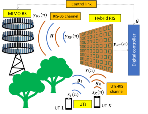
Figure 3: The considered HRIS-empowered multi-user MIMO communication system operating in the uplink direction.

II-C HRIS-Assisted Channel Sounding

In order to investigate the capabilities of HRISs in facilitating multi-user wireless communications, we henceforth study the problem of channel estimation in RIS-empowered systems, being one of the main challenges associated with conventional almost passive and reflective RISs [19, 33]. In particular, we consider an uplink multi-user MIMO system, where a BS equipped with $M$ antenna elements serves $K$ single antenna UTs with the assistance of a HRIS, as illustrated in Fig. 3. We assume that there is no direct link between the BS and any of $K$ UTs, and thus communication is done only via the HRIS. Let ${\boldsymbol{H}}\in\mathbb{C}^{M\times N}$ denote the channel gain matrix between the BS and HRIS, and ${{\boldsymbol{g}}}_{k}\in\mathbb{C}^{N}$ be the channel gian vector between the $k$-th UT ($k=1,2,\ldots,K$) and HRIS. We consider independent and identically distributed (i.i.d.) Rayleigh fading for all channels with ${\boldsymbol{H}}$ and each ${{\boldsymbol{g}}}_{k}$ having i.i.d. zero-mean Gaussian entries with variances $\beta$ and $\gamma_{k}$, respectively, denoting the path losses. In addition, for notation simplicity, we define the matrix ${{\boldsymbol{G}}}\triangleq\left[{{\boldsymbol{g}}}_{1},\cdots,{{\boldsymbol{g}}}_{K}\right]$.

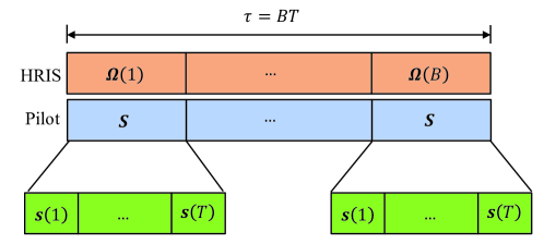
Figure 4: The frame structure for channel estimation using the proposed HRIS.

We consider a simple pilot-based channel training protocol, where the channel estimation time $\tau$ is divided into $B$ sub-frames, and each sub-frame consists of $T$ times slots such that $\tau=BT$, as depicted in Fig. 4. The reconfigurable parameters of the HRIS remain constant during each sub-frame of $T$ time slots and vary from one sub-frame to another. Orthogonal pilot sequences $\left\{{\boldsymbol{s}}_{k}\right\}_{k=1}^{K}$ are sent repeatedly over the $B$ sub-frames, where ${\boldsymbol{s}}_{k}\triangleq\left[s_{k}\left(1\right),s_{k}\left(2\right),\ldots,s_{k}\left(T\right)\right]\in\mathbb{C}^{1\times T}$ is the pilot sequence of the $k$-th UT satisfying for for $1\leq k_{1},k_{2}\leq K$: ${\boldsymbol{s}}_{k_{1}}{\boldsymbol{s}}_{k_{2}}^{H}=T$, if $k_{1}=k_{2}$; and ${\boldsymbol{s}}_{k_{1}}{\boldsymbol{s}}_{k_{2}}^{H}=0$, if $k_{1}\neq k_{2}$. In Fig. 4, ${\boldsymbol{s}}(t)\triangleq\left[s_{1}\left(t\right),s_{2}\left(t\right),\ldots,s_{K}\left(t\right)\right]^{T}$ collects the pilot signals of the $K$ UTs at each $t$-th time slot for each sub-frame, and ${\boldsymbol{\Omega}}\left(b\right)\triangleq\left[{\boldsymbol{\rho}}(b),{\boldsymbol{\phi}}(b),{\boldsymbol{\psi}}(b)\right]$ includes all the optimization variables of the HRIS at each $b$-th sub-frame. Consequently, the signal received at the HRIS at each $t$-th time slot for each $b$-th sub-frame is given by:

$${\boldsymbol{y}}_{\rm RC}\left(b,t\right)={\boldsymbol{\Phi}}\left({\boldsymbol{\rho}}(b),{\boldsymbol{\phi}}(b)\right){\boldsymbol{G}}{\boldsymbol{s}}(t)+{\boldsymbol{z}}_{\rm RC}\left(b,t\right),$$ (5)

where ${\boldsymbol{\Phi}}\left({\boldsymbol{\rho}}(b),{\boldsymbol{\phi}}(b)\right)$ represents the reception matrix of the HRIS during the $b$-th sub-frame and ${\boldsymbol{z}}_{\rm RC}\left(b,t\right)\in\mathbb{C}^{N_{r}}$ is a zero-mean Additive White Gaussian Noise (AWGN) with entries having the variance $\sigma_{\rm RC}^{2}$. Similar to the derivation of (5), the signal received at the BS at each $t$-th time slot for each $b$-th sub-frame can be expressed as:

$${\boldsymbol{y}}_{\rm BS}\left(b,t\right)={\boldsymbol{H}}{\boldsymbol{\Psi}}\left({\boldsymbol{\rho}}(b),{\boldsymbol{\psi}}(b)\right)\,{\boldsymbol{G}}{\boldsymbol{s}}(t)+{\boldsymbol{z}}_{\rm BS}\left(b,t\right),$$ (6)

where ${\boldsymbol{z}}_{\rm BS}\left(b,t\right)\in\mathbb{C}^{M}$ is a zero-mean AWGN having i.i.d. elements each with variance $\sigma_{\rm BS}^{2}$.

Let ${\boldsymbol{y}}_{\rm RC}\left(b\right)\triangleq\left[{\boldsymbol{y}}_{\rm RC}\left(b,1\right),{\boldsymbol{y}}_{\rm RC}\left(b,2\right),\ldots,{\boldsymbol{y}}_{\rm RC}\left(b,T\right)\right]\in\mathbb{C}^{N_{r}\times T}$ be the matrix collecting the received signals at the HRIS over $T$ time slots for each $b$-th block, i.e.:

$${\boldsymbol{y}}_{\rm RC}\left(b\right)={\boldsymbol{\Phi}}\left({\boldsymbol{\rho}}(b),{\boldsymbol{\phi}}(b)\right){\boldsymbol{G}}{\boldsymbol{S}}+{\boldsymbol{z}}_{\rm RC}\left(b\right),$$ (7)

with ${\boldsymbol{z}}_{\rm RC}\left(b\right)\triangleq\left[{\boldsymbol{z}}_{\rm RC}\left(b,1\right),{\boldsymbol{z}}_{\rm RC}\left(b,2\right),\ldots,{\boldsymbol{z}}_{\rm RC}\left(b,T\right)\right]\in\mathbb{C}^{N_{r}\times T}$ and ${\boldsymbol{S}}\triangleq\left[{\boldsymbol{s}}(1),{\boldsymbol{s}}(2),\ldots,{\boldsymbol{s}}(T)\right]$, where it holds that ${\boldsymbol{S}}{\boldsymbol{S}}^{H}=T{\bf I}_{K}$. We, then, define ${\boldsymbol{y}}_{\rm RC}$ as the $N_{r}\,B\times T$ matrix generated by stacking the rows of the $B$ matrices ${\boldsymbol{y}}_{\rm RC}\left(1\right),{\boldsymbol{y}}_{\rm RC}\left(2\right),\ldots,{\boldsymbol{y}}_{\rm RC}\left(B\right)$. From (7), ${\boldsymbol{y}}_{\rm RC}$ can be written as a linear function of the UTs-HRIS channel ${\boldsymbol{G}}$ as

$${\boldsymbol{y}}_{\rm RC}={\boldsymbol{A}}_{\rm RC}\left(\left\{{\boldsymbol{\rho}}(b),{\boldsymbol{\phi}}(b)\right\}\right){{\boldsymbol{G}}}{\boldsymbol{S}}+{\boldsymbol{z}}_{\rm RC},$$ (8)

where ${\boldsymbol{z}}_{\rm RC}\in\mathbb{C}^{N_{r}\,B\times T}$ results from the row stacking of the matrices ${\boldsymbol{z}}_{\rm RC}(1),{\boldsymbol{z}}_{\rm RC}(2),\ldots,{\boldsymbol{z}}_{\rm RC}(B)$, while the matrix ${\boldsymbol{A}}_{\rm RC}\in\mathbb{C}^{N_{r}\,B\times N}$ is defined as:

$${\boldsymbol{A}}_{\rm RC}\left(\left\{{\boldsymbol{\rho}}(b),{\boldsymbol{\phi}}(b)\right\}\right)\triangleq\left[{\boldsymbol{\Phi}}\left({\boldsymbol{\rho}}(1),{\boldsymbol{\phi}}(1)\right)^{T},\cdots,{\boldsymbol{\Phi}}\left({\boldsymbol{\rho}}(B),{\boldsymbol{\phi}}(B)\right)^{T}\right]^{T}.$$ (9)

Similarly, by letting ${\boldsymbol{y}}_{\rm BS}\left(b\right)\triangleq\left[{\boldsymbol{y}}_{\rm BS}\left(b,1\right),{\boldsymbol{y}}_{\rm BS}\left(b,2\right),\ldots,{\boldsymbol{y}}_{\rm BS}\left(b,T\right)\right]\in\mathbb{C}^{M\times T}$ be the matrix including the received signals at BS during the $T$ time slots for each $b$-th sub-frame, we have:

$${\boldsymbol{y}}_{\rm BS}\left(b\right)={\boldsymbol{H}}{\boldsymbol{\Psi}}\left({\boldsymbol{\rho}}(b),{\boldsymbol{\psi}}(b)\right){\boldsymbol{G}}{\boldsymbol{S}}+{\boldsymbol{z}}_{\rm BS}\left(b\right),$$ (10)

where ${\boldsymbol{z}}_{\rm BS}\left(b\right)\triangleq\left[{\boldsymbol{z}}_{\rm BS}\left(b,1\right),{\boldsymbol{z}}_{\rm BS}\left(b,2\right),\ldots,{\boldsymbol{z}}_{\rm BS}\left(b,T\right)\right]\in\mathbb{C}^{M\times T}$.

As in conventional RIS-empowered communication systems, e.g., [4, 39], we assume that the BS maintains a high-throughput direct link with the HRIS. For passive RISs, this link is used for controlling the RIS reflection pattern. In HRISs, which have reception, thus measurement collection, capabilities, this link is also used for conveying valuable information from the HRIS to the BS. Therefore, inspired by the recent discussions for autonomous RISs with basic computing and storage capabilities [40, 41], we focus on channel estimation carried out at both the HRIS side as well as the BS. Our goal is to characterize the achievable MSE in recovering the UTs-HRIS channel ${\boldsymbol{G}}$ from (8), along with the MSE in estimating ${\boldsymbol{H}}$ at the BS from (10) and from the estimate of ${\boldsymbol{G}}$, denoted $\hat{{\boldsymbol{G}}}$, provided by the HRIS. The pilot matrix ${\boldsymbol{S}}$ in (8) and (10) is assumed to be known at both the HRIS and BS. It ia also noted that different HRIS configurations $\left\{{\boldsymbol{\rho}}(b),{\boldsymbol{\phi}}(b),{\boldsymbol{\psi}}(b)\right\}$ result in different pilot signal strengths in (8) and (10). Therefore, we also aim at configuring the HRIS controllable parameters in order to facilitate channel estimation based on the characterized MSE.

III Estimation of the Individual Channels

In this section, we quantify the HRIS potential in facilitating estimation of all individual channels in the uplink of HRIS-empowered multi-user MIMO communication systems. In the considered model, the individual UTs-HRIS channel is estimated at the HRIS side based on (8), while the individual HRIS-BS channel is estimated at the BS from (10) using the estimation $\hat{{\boldsymbol{G}}}$, which is provided by the HRIS. In this section, we first study the number of pilots needed to estimate the channels for a noise-free setting in Subsection III-A, where ${\boldsymbol{G}}$ and ${\boldsymbol{H}}$ can be identified with no errors. Then, we express the achievable channel estimation MSE for noisy reception in Subsection III-B, which we then use to optimize the HRIS in Subsection III-C. A discussion on the proposed channel estimation approach is provided in Subsection III-D.

III-A Channel Estimation for Noise-Free Channels

We begin by considering communications carried out in the case of without noise, where the noise terms in (5) and (6) are set to be zero, i.e., $\sigma_{\rm RC}^{2}=\sigma_{\rm BS}^{2}=0$. In such scenarios, one should be able to fully recover both ${\boldsymbol{H}}$ and ${\boldsymbol{G}}$ from the observed signals ${\boldsymbol{y}}_{\rm RC}(n)$ and ${\boldsymbol{y}}_{\rm BS}(n)$. The number of pilots required to achieve accurate recovery is stated in the following proposition.

Proposition 1.

In the case of without noise, ${\boldsymbol{H}}$ and ${\boldsymbol{G}}$ can be accurately recovered when the number of pilots $\tau$ satisfies the inequality:

$$\tau\geq N\cdot\max\left\{1,KN_{r}^{-1}\right\}.$$ (11)

Proof:

The proof is provided in Appendix A. ∎

Proposition 1 demonstrates the intuitive benefit of HRISs in facilitating individual channel estimation with reduced number of pilots, as compared to existing techniques for estimating the cascaded UTs-RIS-BS channels (e.g., [17]). For instance, for a multi-user MIMO system with $M=16$ BS antennas, $N_{r}=8$ HRIS RF chains, $K=8$ UTs, and $N=64$ HRIS elements, the adoption of an HRIS allows recovering ${\boldsymbol{H}}$ and ${\boldsymbol{G}}$ separately using $\tau=64$ pilots. By contrast, the method proposed in [17] requires transmitting over $90$ pilots to identify the cascaded channel coefficients $[{\boldsymbol{H}}]_{m,l}[{\boldsymbol{G}}]_{l,k}$ for $l,k$ and $m=1,2,\ldots,M$. This reduction in pilot signals is directly translated into improved spectral efficiency, as less pilots are to be transmitted in each coherence duration.

III-B Channel Estimation for Noisy Channels

The characterization of the number of required pilots in Proposition 1 provides an initial understanding of the HRIS’s capability in providing efficient channel estimation. However, as Proposition 1 considers an effectively noise-free setup, it is invariant of the fact that HRISs split the power of their received signal ${\boldsymbol{r}}(n)$ between the reflected and received components. In the presence of noise, this division of the signal power may result in Signal-to-Noise Ratio (SNR) degradation. Therefore, we next study channel estimation using HRISs in the presence of noise, quantifying the achievable MSE in estimating the individual UTs-HRIS and HRIS-BS channels for a fixed HRIS configuration $\left\{{\boldsymbol{\rho}}(b),{\boldsymbol{\phi}}(b),{\boldsymbol{\psi}}(b)\right\}$. For notation brevity, in the following, we define the set of HRIS parameters affecting its reception as ${\boldsymbol{\Phi}}\triangleq\left\{{\boldsymbol{\rho}}(b),{\boldsymbol{\phi}}(b)\right\}$, the HRIS parameters affecting the reception at the BS as ${\boldsymbol{\Psi}}(b)\triangleq{\boldsymbol{\Psi}}({\boldsymbol{\rho}}(b),{\boldsymbol{\psi}}(b))$, and the overall HRIS parameters as ${\boldsymbol{\Omega}}\triangleq\left\{{\boldsymbol{\rho}}(b),{\boldsymbol{\phi}}(b),{\boldsymbol{\psi}}(b)\right\}$. We also make the assumption that the noise powers at the HRIS and BS are of the same level, i.e., $\sigma_{\rm BS}^{2}=\sigma_{\rm RC}^{2}=\sigma^{2}$.

We begin by characterizing the achievable MSE performance in recovering ${\boldsymbol{G}}$ at the HRIS using its locally collected measurements for a given HRIS parameterization, denoted by $\mathcal{E}_{{\boldsymbol{G}}}\left({\boldsymbol{\Phi}}\right)$.

Theorem 1.

The UTs-HRIS channel ${\boldsymbol{G}}$ can be recovered with the following MSE performance:

$$\mathcal{E}_{{\boldsymbol{G}}}\left({\boldsymbol{\Phi}}\right)={\rm Tr}\left\{\left({\boldsymbol{R}}_{\rm G}^{-1}\,+T\frac{\Gamma}{K}{\boldsymbol{A}}_{\rm RC}\left({\boldsymbol{\Phi}}\right)^{H}\,{\boldsymbol{A}}_{\rm RC}\left({\boldsymbol{\Phi}}\right)\right)^{-1}\right\}$$

where ${\boldsymbol{R}}_{\rm G}\triangleq\left(\sum_{k=1}^{K}\gamma_{k}\right){\boldsymbol{I}}_{N}$; $\Gamma\triangleq\frac{P_{t}}{\sigma^{2}}$ represents the transmit SNR with $P_{t}$ denoting each UT’s power used for transmitted the pilot symbols.

Proof:

The proof is given in Appendix B. ∎

Theorem 1 allows to compute the achievable MSE in estimating ${\boldsymbol{G}}$ at the HRIS side for a given configuration of its reception phase profile, determined by ${\boldsymbol{\Phi}}$, i.e., by $\left\{{\boldsymbol{\rho}}(b)\right\}$ and $\left\{{\boldsymbol{\phi}}(b)\right\}$.

Lemma 1.

Let ${\boldsymbol{\hat{G}}}$ and ${\boldsymbol{\tilde{G}}}={\boldsymbol{G}}-{\boldsymbol{\hat{G}}}$ denote the estimation of ${\boldsymbol{G}}$ and its corresponding estimation error, respectively. From Appendix B, the distributions of ${\boldsymbol{\hat{G}}}$ and ${\boldsymbol{\tilde{G}}}$ are respectively given by

$${\boldsymbol{\hat{G}}}\sim\mathcal{C}\mathcal{N}\left(0,{\boldsymbol{\Sigma}}\left({\boldsymbol{\Phi}}\right)\right),\qquad{\boldsymbol{\tilde{G}}}\sim\mathcal{C}\mathcal{N}\left(0,{\boldsymbol{R}}_{\bf\tilde{G}}\left({\boldsymbol{\Phi}}\right)\right),$$

where ${\boldsymbol{R}}_{\bf\tilde{G}}\left({\boldsymbol{\Phi}}\right)$ and ${\boldsymbol{\Sigma}}\left({\boldsymbol{\Phi}}\right)$ are defined as ${\boldsymbol{R}}_{\bf\tilde{G}}\left({\boldsymbol{\Phi}}\right)\triangleq\left({\boldsymbol{R}}_{\rm G}^{-1}\,+T\Gamma K^{-1}\,{\boldsymbol{A}}_{\rm RC}\left({\boldsymbol{\Phi}}\right)^{H}\,{\boldsymbol{A}}_{\rm RC}\left({\boldsymbol{\Phi}}\right)\right)^{-1}$ and ${\boldsymbol{\Sigma}}\triangleq{\boldsymbol{R}}_{\rm G}\,{\boldsymbol{A}}_{\rm RC}\left({\boldsymbol{\Phi}}\right)^{H}\,\Bigg{(}{\boldsymbol{A}}_{\rm RC}\left({\boldsymbol{\Phi}}\right)\,{\boldsymbol{R}}_{\rm G}\,{\boldsymbol{A}}_{\rm RC}\left({\boldsymbol{\Phi}}\right)^{H}+K\,(T\Gamma)^{-1}\,{{\boldsymbol{I}}_{N_{r}B}}\Bigg{)}^{-1}{\boldsymbol{A}}_{\rm RC}\left({\boldsymbol{\Phi}}\right){\boldsymbol{R}}_{\rm G}^{H}$.

Lemma 1 provides the statistical results for the estimation of ${\boldsymbol{G}}$ with respect to the reconfigurable parameters ${\boldsymbol{\Phi}}$; more specifically, to $\left\{{\boldsymbol{\rho}}(b)\right\}$ and $\left\{{\boldsymbol{\phi}}(b)\right\}$. This estimation can be used from the BS to estimate the channel matrix ${\boldsymbol{H}}$. In particular, letting the HRIS convey the estimation of ${\boldsymbol{G}}$ to the BS (via their control link) allows achieving the MSE in recovering ${\boldsymbol{H}}$, as described by means of the following theorem. Recall that the BS observes the reflected portion of the signal at the output of the HRIS-BS channel.

Theorem 2.

The HRIS-BS channel ${\boldsymbol{H}}$ can be recovered with the following MSE performance:

$$\mathcal{E}_{{\boldsymbol{H}}}\left({\boldsymbol{\Omega}}\right)={\rm Tr}\left(\left(\frac{1}{\beta}{\boldsymbol{I}}_{MN}+\left(K\sum_{j=1}^{B}\sum_{i=1}^{B}\,{\rm Tr}\left(\left[{\boldsymbol{D}}({\boldsymbol{\Omega}})^{-T}\right]_{i,j}\right)\,{\boldsymbol{\Psi}}(i)\,{\boldsymbol{\Sigma}}\left({\boldsymbol{\Phi}}\right){\boldsymbol{\Psi}}(j)^{H}\right)^{T}\otimes{\boldsymbol{I}}_{M}\right)^{-1}\right),$$

where ${\boldsymbol{D}}({\boldsymbol{\Omega}})$ is a ${BK\times BK}$ matrix which can be partitioned into $B\times B$ blocks with each block being a $K\times K$ submatrix. The $i$-th row and $j$-th column block of ${\boldsymbol{D}}({\boldsymbol{\Omega}})$ is defined as:

$$\begin{split}&\left[{\boldsymbol{D}}\left({\boldsymbol{\Omega}}\right)\right]_{i,j}=\left\{\begin{array}[]{ll}\frac{\beta}{K}{\rm Tr}\left({\boldsymbol{\Psi}}(j)^{H}{\boldsymbol{\Psi}}(i){\boldsymbol{R}}_{\bf\tilde{G}}\left({\boldsymbol{\Phi}}\right)\right){\boldsymbol{I}}_{K}+(T\Gamma)^{-1}{\boldsymbol{I}}_{K},&{\rm if}~{}i=j\\ \frac{\beta}{K}{\rm Tr}\left({\boldsymbol{\Psi}}(j)^{H}{\boldsymbol{\Psi}}(i){\boldsymbol{R}}_{\bf\tilde{G}}\left({\boldsymbol{\Phi}}\right)\right){\boldsymbol{I}}_{K},&{\rm if}~{}i\neq j\end{array}\right..\end{split}$$

Proof:

The proof is provided in Appendix C. ∎

Theorems 1 and 2 allow us to evaluate the achievable MSE for the recovery of the individual channels ${\boldsymbol{G}}$ and ${\boldsymbol{H}}$. The fact that these MSEs are given as functions of the HRIS parameters ${\boldsymbol{\Omega}}$ enables us to numerically optimize the HRIS configuration for the estimation of the individual channels. In Section IV, our numerical evaluation of the MSE performance reveals the fundamental trade-off between the ability to recover ${\boldsymbol{G}}$ and ${\boldsymbol{H}}$, which is dictated mostly by the parameter ${\boldsymbol{\rho}}$ determining the portion of the impinging signal being reflected; the remaining portion is sensed and used for channel estimation at the HRIS side.

III-C HRIS Configuration Optimization

The formulation of the channel estimation MSE given previously for a fixed HRIS configuration motivates the optimization of its parameters. We henceforth seek to optimize the HRIS parameters ${\boldsymbol{\Omega}}=\left\{\boldsymbol{\rho}\left(b\right),\boldsymbol{\psi}\left(b\right),\boldsymbol{\phi}\left(b\right)\right\}$ so as to minimize the weighted-sum MSE. Mathematically, the optimization problem under investigation is formulated as follows:

$$\begin{split}&\min_{\left\{\boldsymbol{\rho}\left(b\right),\boldsymbol{\psi}\left(b\right),\boldsymbol{\phi}\left(b\right)\right\}}~{}~{}\mathcal{E}_{{\boldsymbol{H}}}\left(\left\{\boldsymbol{\rho}\left(b\right),\boldsymbol{\psi}\left(b\right),\boldsymbol{\phi}\left(b\right)\right\}\right)+\mathcal{E}_{{\boldsymbol{G}}}\left(\left\{\boldsymbol{\rho}(b),\boldsymbol{\phi}(b)\right\}\right)\\ &~{}~{}~{}~{}~{}~{}s.t.~{}~{}~{}~{}~{}~{}~{}~{}~{}~{}[{\boldsymbol{\rho}}(b)]_{p}\in[0,1],~{}[{\boldsymbol{\psi}}(b)]_{p}\in[0,2\pi],~{}[{\boldsymbol{\phi}}(b)]_{q}\in[0,2\pi],~{}\\ &~{}~{}~{}~{}~{}~{}~{}~{}~{}~{}~{}~{}~{}~{}~{}~{}~{}~{}~{}~{}b=1,2,\ldots,B,~{}p=1,2,\ldots,N,~{}q=1,2,\ldots,N\times N_{r}.\end{split}$$ (12)

Problem (12) is non-convex and challenging to solve, even when using numerical approaches based on Bayesian optimization, as previously proposed for RIS configuration in complex settings [42]. This is because the dimension of the optimization variables is extremely high when the number of antennas at the BS and the number of meta-atom elements at the HRIS are large. We thus propose to tackle the HRIS reconfiguration problem in (12) via a gradient-based optimization approach.

The gradients of the sum-MSE objective function with respect to the HRIS parameters can be computed analytically with AD [43], which is extensively used for machine learning applications. To compute the gradients of a differentiable function automatically, AD expresses the function as a computational graph and applies the backpropagation algorithm to retrieve the gradients. To justify the use of AD, we recall that the sum-MSE objective function is composed of basic differentiable operations, such as the matrix trace operation. Moreover, the composition of differentiable functions results in a differentiable function, and thus the sum-MSE objective function is differentiable, allowing us to apply AD.

For notation brevity, in the following, we define $f\left(\mathbf{x}\right)$ as the objective function of (12) with $\mathbf{x}\triangleq\left[{\boldsymbol{\rho}}\left(1\right),\ldots,\boldsymbol{\rho}\left(B\right),{{\boldsymbol{\psi}}}\left(1\right),\ldots,{\boldsymbol{\psi}}\left(B\right),{{\boldsymbol{\phi}}}\left(1\right),\ldots,{\boldsymbol{\phi}}\left(B\right)\right]$ including the elements of the set ${\boldsymbol{\Omega}}$ of the HRIS parameters in a vector form. To deal with the inequality constraints on the HRIS free variables, we add a barrier regularization term to the objective function of (12), resulting in the following optimization problem:

$$\min_{\mathbf{x}\in\mathcal{C}}~{}~{}~{}\mathcal{L}(\mathbf{x})\triangleq f(\mathbf{x})+\lambda\mathcal{B}_{\mathcal{C}}(\mathbf{x}).$$ (13)

where $\lambda\in\mathbb{R}$ is a regularization hyperparameter, $\mathcal{C}$ denotes the feasible set of $\mathbf{x}$, given by equation $\mathcal{C}\triangleq\left\{\mathbf{x}\in\mathbb{R}^{BN\left(2+N_{r}\right)}:0\leq\mathbf{x}_{i}\leq 1,\forall i\in\left[1,BN\right]~{}{\rm and}~{}0\leq\mathbf{x}_{i}\leq 2\pi,\forall i\in\left[BN+1,BN\left(2+N_{r}\right)\right]\right\}$, and $\mathcal{B}_{\mathcal{C}}(\mathbf{x})$ represents the barrier function, which adds a high penalty to the points approaching the feasible region’s boundaries. Formally, a barrier function $\mathcal{B}_{\mathcal{C}}(\mathbf{x})$ is any function that satisfies: i) $\mathcal{B}_{\mathcal{C}}(\mathbf{x})\geq 0$ $\forall\mathbf{x}\in\mathcal{C}$; and ii) $\mathcal{B}_{\mathcal{C}}(\mathbf{x})\rightarrow\infty$ $\forall\mathbf{x}\rightarrow\partial\mathcal{C}$, where $\partial\mathcal{C}$ denotes the boundaries of the feasible region. In the problem formulation in (13), we adopt the barrier function:

$$\mathcal{B}_{\mathcal{C}}(\mathbf{x})=\sum_{i=1}^{BN}\left(\frac{1}{\mathbf{x}_{i}}+\frac{1}{1-\mathbf{x}_{i}}\right)+\sum_{i=BN+1}^{BN\left(2+N_{r}\right)}\left(\frac{1}{\mathbf{x}_{i}}+\frac{1}{2\pi-\mathbf{x}_{i}}\right),$$ (14)

which is differentiable, returns non-negative values in the feasible set, and is not bounded as the variables approach the feasible set’s boundaries. To solve the resulting minimization problem, we apply a gradient-based iterative approach, where at each iteration we compute the derivative with an AD tool (we used PyTorch’s autograd engine [44]) and update the parameters with a first-order optimizer (e.g., gradient descent and its variants, such as Adam [45]). The solution using a conventional gradient descent algorithm with AD is summarized in Algorithm 1.

Algorithm 1 HRIS Configuration for Weighted-Sum MSE Minimization

0:  $\mathbf{x}^{(0)}$, step-size $\eta$, and $t\leftarrow 0$.

1:  while stopping criteria is not satisfied do

2:     Update the objective value $\mathcal{L}(\mathbf{x})$ in (13).

3:     Compute the gradients using the AD-based backpropagation algorithm $\nabla_{\mathbf{x}}\mathcal{L}(\mathbf{x}^{(t)})$.

4:     Update the parameters vector via $\mathbf{x}^{(t+1)}\leftarrow\mathbf{x}^{(t)}-\eta\nabla_{\mathbf{x}}\mathcal{L}(\mathbf{x}^{(t)})$.

5:     Update $t\leftarrow t+1$.

6:  end while

6:  $\left\{\boldsymbol{\rho}\left(b\right),\boldsymbol{\psi}\left(b\right),\boldsymbol{\phi}\left(b\right)\right\}\leftarrow\mathbf{x}^{(t)}$.

III-D Discussion

The fact that HRISs require less pilots naturally follows from their ability to provide additional $N_{r}$ reception ports, while simultaneously acting as a dynamically configurable reflector. It is noted that our results in the previous subsections are obtained assuming that the UTs-HRIS channel ${\boldsymbol{G}}$ is estimated at the HRIS, and its estimate is then forwarded to the BS. Furthermore, exploiting the HRIS as an additional non-co-located receive port can also facilitate data transmission once the channels are estimated. Though, in this case, one would also have to account for possible rate limitations on the HRIS-BS link. We leave the study of these additional usages of HRISs for future research.

The study of HRISs, combined with the numerical evaluations in Section IV that follows, only reveal a portion of the potential of HRISs in facilitating wireless communication over programmable environments. To further understand the contribution of HRISs, one should also study their impact on data transmission, as well as consider the presence of an additional direct channel between the UTs and the BS. Furthermore, the simplified model used in this work is based on the hybrid metamaterial model presented in [31]. To this end, additional experimental studies of this model are required to formulate a more accurate physically-compliant model for the behavior of HRISs; see [46] and references therein for recent modeling research. These extensions are also left for future work.

Our proposed hybrid RIS structure is different from another emerging hybrid RIS concept, called simultaneously transmitting and reflecting (STAR)-RIS [36, 35, 34]. In STAR-RIS, each antenna element splits its incident signal power into two parts, i.e., one part of the signal is reflected in the same space as the incident signal, and the other part of the signal is transmitted to the opposite space of the incident signal. Hence, STAR-RIS is capable of simultaneous reflection and refraction (passing the signal through the surface to its other side), without having any receiving or decoding capability.

IV Numerical Results

In this section, we numerically evaluate the performance of the proposed channel estimation approach for the uplink of HRIS-empowered multi-user MIMO communication systems. Specifically, we present simulation parameters in Section IV-A and then provide our numerical results in Section IV-B.

IV-A Simulation Setup

In our simulations, the pathlosses of the individual channels ${\bf H}$ and ${\bf g}_{k}$ are modeled as $\beta=\lambda_{0}\left(\frac{d_{H}}{d_{0}}\right)^{-\alpha_{h}}$ and $\gamma_{k}=\lambda_{0}\left(\frac{d_{k}}{d_{0}}\right)^{-\alpha_{g}}$, respectively, where $\lambda_{0}=-20$ dB denotes a constant pathloss at the reference distance $d_{0}=1$ m, while $d_{H}$ and $d_{k}$ are the distances from the HRIS to the BS and $k$th UT, respectively. The pathloss exponents were set as $\alpha_{h}=2.2$ and $\alpha_{g}=2.1$. The above wireless channel parameters were also adopted in [17]. We consider a 2D Cartesian coordinate system in which the BS and the HRIS are respectively located at points (0, 0) and (0, 50 m), while the $K$ users were randomly generated in an area centered at (30 m, 50 m) with a radius of $10$ m. In addition, we have set the numbers of antennas at the BS and the number of meta-atom elements at the HRIS as $M=16$ and $N=64$, respectively, and the number of UTs as $K=8$, unless otherwise stated.

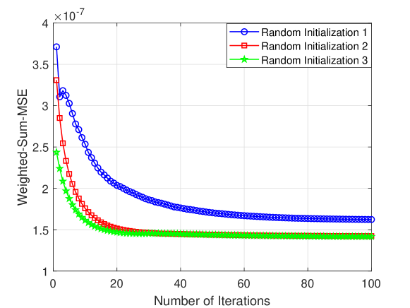
Figure 5: Convergence behavior of the weighted-sum MSE for the proposed channel estimation algorithm with different random initialization using $N_{r}=8$ receive RF chains at the HRIS, transmit SNR of $\Gamma=100$ dB, and $\tau=104$ pilots symbols.

IV-B Simulation Results

We first demonstrate the convergence behavior of our proposed AD-based Algorithm 1 for solving the considered channel estimation problem. Specifically, Fig. 5 depicts the convergence of the achievable weighted sum-MSE for different random initialization of the optimization variables, when the number of receive RF chains at the HRIS is set to $N_{r}=8$, the transmit SNR $\Gamma=100$ dB, and the pilot length is $\tau=104$. It can be observed that for each randomly generated initialization, the proposed algorithm converges to a fixed value within $100$ iterations, and typically with much fewer iterations, verifying its relatively fast convergence. Therefore, we have set the maximum number of iterations to be $100$ for Algorithm 1 in the following simulation experiments.

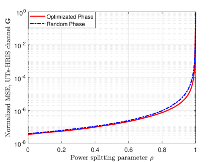
(a) Normalized MSE of estimating the UTs-HRIS channel ${\bf G}$.

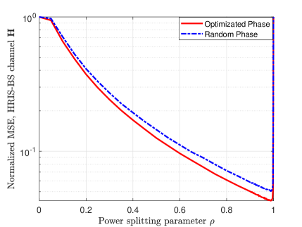
(b) Normalized MSE of estimating the HRIS-BS channel ${\bf H}$.

Figure 6: Normalized MSE performance of the proposed channel estimation algorithm in recovering the combined UTs-HRIS channel ${\bf G}$ at the HRIS and the HRIS-BS channel ${\bf H}$ at the BS using $\tau=104$ pilots symbols.

In Fig. 6, we show the trade-off between the normalized MSE performances when estimating the UTs-HRIS channel ${\bf G}$ at the HRIS and the HRIS-BS channel ${\bf H}$ at the BS for different values of the power splitting parameter $\rho$; we have assumed that all the elements of the HRIS have the same power splitting parameter $\rho$. In the figure, we have set the transmit SNR to $\Gamma=100$ dB and the pilot length $\tau=104$. In addition, “Optimized Phase” denotes that the phase variables of the HRIS have been optimized using Algorithm 1, and “Random Phase” indicates that the HRIS phase variables were generated randomly. It can be observed from Fig. 6(a) that the normalized MSE of estimating the individual channel ${\bf G}$ increases significantly as $\rho$ increases. This happens because as $\rho$ increases, each meta-atoms element of the HRIS splits less power of the impinging signal for channel estimation. It is also shown in Fig. 6(b) that as $\rho$ increases, the normalized MSE of estimating the individual channel ${\bf H}$ decreases gradually. This improvement ceases when $\rho$ approaches $1$, implying that the HRIS behaves as a purely passive RIS and the individual channels cannot be disentangled. This clearly demonstrates the fundamental trade-off between the accuracy in estimating each of the individual channels, which is dictated by the way that the HRIS splits the power of the impinging signal. In addition, it is evident from the figure that the channel estimation performance of the “Optimized Phase” case is slightly better than that of the “Random Phase,” especially when the power splitting parameter $\rho$ approaches its maximum value. This performance enhancement will become more significant when also optimizing the power splitting parameter $\rho$, as will be demonstrated in the sequel.

We now compare the channel estimation performance, considering our proposed HRIS-based approach (labeled as “Proposed HRIS”), the existing passive reflective RIS-based approach of [17] (labeled as “Reflective RIS”), and two baseline schemes (labeled as “Proposed HRIS with Partial Connection” and “Proposed HRIS with Random Parameters”). The former baseline scheme adopts a partially-connected analog combiner at the HRIS receiver, i.e., each antenna element just connects to only one receive RF chain, like the DMA structure defined in [26], and the corresponding power splitting parameters and phase configurations are optimized using Algorithm 1. With the latter baseline scheme, the power splitting parameters and phase profiles are randomly generated within the feasible set. In addition, since the channel estimation approach proposed in [17] can only estimate the cascaded channel, we also calculated the resulting cascaded channel estimation for the proposed approach, using our estimated individual BS-HRIS channel ${\boldsymbol{\hat{H}}}$ and the UTs-HRIS channel ${\boldsymbol{\hat{G}}}=[{{\boldsymbol{\hat{g}}}}_{1},{{\boldsymbol{\hat{g}}}}_{2},\ldots,{{\boldsymbol{\hat{g}}}}_{K}]$. Specifically, the normalized MSE performance of the estimated cascaded channel with our HRIS-based approach was calculated as follows:

$$\operatorname{e}^{c}\triangleq\frac{\mathbb{E}\left\{\sum_{k=1}^{K}\left\|{\boldsymbol{\hat{H}}}{\rm diag}\left({{\boldsymbol{\hat{g}}}}_{k}\right)-{\boldsymbol{H}}{\rm diag}\left({{\boldsymbol{g}}}_{k}\right)\right\|_{F}^{2}\right\}}{\mathbb{E}\left\{\sum_{k=1}^{K}\left\|{\boldsymbol{H}}{\rm diag}\left({{\boldsymbol{g}}}_{k}\right)\right\|_{F}^{2}\right\}}.$$ (15)

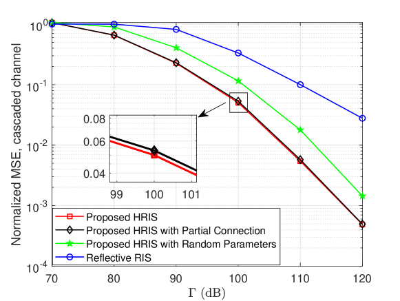
Figure 7: Normalized MSE performance of the cascaded channel estimation versus the transmit SNR $\Gamma$ for $\tau=104$ pilots symbols for each of the $K=8$ UTs. Various versions of the proposed HRIS with $N_{r}=8$ receive RF chains and a reflective RIS have been considered.

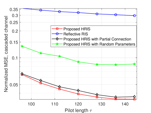
Figure 8: Normalized MSE performance of the cascaded channel estimation versus the pilot symbols’ length $\tau$ used by each of the $K=8$ UTs, considering the transmit SNR $\Gamma=100$ dB. All schemes compared in Fig. (7) have been considered.

In Fig. 7, we demonstrate the normalized MSE of the cascaded channel estimation as a function of the transmit SNR value $\Gamma$ for the considered estimation methods, using $N_{r}=8$ receive RF chains for our HRIS architecture. The method “Reflective RIS” in [17] was found to require at least $92$ pilot symbols, and thus, we set the pilot length to $\tau=104$. As shown in the figure, the HRISs sensing capability is translated into improved cascaded channel estimation accuracy, as compared to the state of the art. For example, the proposed HRISs (even with the random configuration case “Proposed HRIS with Random Parameters”) can achieve a much lower normalized MSE than that of the “Relective RIS.” In addition, it can be observed that the performance of the case “Proposed HRIS with Partial Connection” is comparable with that of the “Proposed HRIS,” which indicates the effectiveness of our proposed HRIS even when using the lower power consumption and hardware complexity partially-connected analog combiner.

We also plot the normalized MSE of the cascaded channel against the pilot sequence length $\tau$ in Fig. 8, considering the transmit SNR value $\Gamma=100$ dB and $N_{r}=8$ received RF chains at the HRIS. Evidently, the proposed HRIS-based approaches can significantly reduce the error of the cascaded channel estimation, as compared to the passive reflection RIS. Moreover, we see that for the proposed HRIS, the normalized MSE decreases rapidly at first and then tends to slow down as the pilot length increases. As before, our proposed HRIS with a partially-connected analog combiner is capable of achieving comparable channel estimation accuracy with that of HRIS with a fully-connected analog combiner.

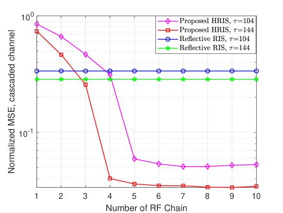
Figure 9: Normalized MSE performance of the cascaded channel estimation versus the number of the receive RF chains $N_{r}$ at the HRIS, considering the transmit SNR $\Gamma=100$ dB and $\tau=\{104,144\}$ pilot symbols’ length at each of the $K=8$ UTs. The proposed HRIS and a reflective RIS are compared.

Finally, in Fig. 9, we investigate the effect of the number $N_{r}$ of receive RF chains on the cascaded channel estimation accuracy, considering the same transmit SNR with Fig. 8 and different pilot sequence lengths $\tau$. It is illustrated that, as $N_{r}$ increases, the normalized cascaded channel MSE decreases initially and then converges to a constant value. This happens because the observed pilot signals increase proportionately to the number of receive RF chains, thereby increasing the accuracy of channel estimation. However, once the observed pilot signals exceed a threshold, increasing their number further will not reduce the channel estimation error. Moreover, it is evident from the figure that the proposed HRIS-based approach achieves higher channel estimation accuracy than the one based on the conventional passive RIS, even when only few receive RF chains are used. For example, in the case of $\tau=104$, the proposed HRIS requires only $N_{r}=5$ receive RF chains to achieve significantly improved channel estimation performance. Additionally, we see that the required $N_{r}$ value decreases as the pilot length increases.

V Conclusion

In this paper, we studied wireless communications aided by HRISs, which are metasurfaces capable of simultaneously reflecting and sensing impinging signals in a dynamically controllable manner. We presented a simple model for the operation of HRIS-empowered multi-user MIMO communications systems, and investigated their potential to facilitate channel estimation, as an indicative application. We showed that for the case without noise, HRISs enable to significantly save pilot overhead compared to that required by purely reflective RISs. We also quantified the achievable estimation error performance for the case with noise. In particular, we derived the individual MSE for estimating individual channels at the HRISs and BS, and proposed a gradient-based approach to configure the HRISs for minimizing the weighted sum-MSE. Our simulation results showcased the impactful role HRISs in RIS-empowered communications in estimating the individual channels as well as the cascaded channel over existing methods relying on nearly passive and reflective RISs.

Appendix A Proof of Proposition 1

By discarding the noise term in (8), the received pilot signal at the HRIS is given by

$${\boldsymbol{y}}_{\rm RC}={\boldsymbol{A}}_{\rm RC}\left(\left\{{\boldsymbol{\rho}}(b),{\boldsymbol{\phi}}(b)\right\}\right){{\boldsymbol{G}}}{\boldsymbol{S}}.$$ (A.1)

By using the identity $\operatorname{vec}(\mathbf{ABC})=\left(\mathbf{C}^{T}\otimes\mathbf{A}\right)\operatorname{vec}(\mathbf{B})$, we can rewrite (A.1) as follows:

$${\operatorname{vec}}\left({\boldsymbol{y}}_{\rm RC}\right)=\left({\boldsymbol{S}}^{T}\otimes{\boldsymbol{A}}_{\rm RC}\left(\left\{{\boldsymbol{\rho}}(b),{\boldsymbol{\phi}}(b)\right\}\right)\right){\rm vec}({\boldsymbol{G}}).$$ (A.2)

In the latter expression, we define ${\boldsymbol{A}}_{\rm 1}\triangleq{\boldsymbol{S}}^{T}\otimes{\boldsymbol{A}}_{\rm RC}\left(\left\{{\boldsymbol{\rho}}(b),{\boldsymbol{\phi}}(b)\right\}\right)$. If ${\boldsymbol{A}}_{\rm 1}$ is a full-column-rank matrix, then $\operatorname{vec}\left({\boldsymbol{G}}\right)$ can be recovered from (A.2) as $\operatorname{vec}\left({\boldsymbol{G}}\right)={\boldsymbol{A}}_{\rm 1}^{\dagger}{\operatorname{vec}}\left({\boldsymbol{y}}_{\rm RC}\right)$, where ${\boldsymbol{A}}_{\rm 1}^{\dagger}=\left({\boldsymbol{A}}_{\rm 1}^{H}{\boldsymbol{A}}_{\rm 1}\right)^{-1}{\boldsymbol{A}}_{\rm 1}^{H}$ is the pseudoinverse of ${\boldsymbol{A}}_{\rm 1}$. Once we obtain the perfect estimate of $\operatorname{vec}\left({\boldsymbol{G}}\right)$, then the channel matrix ${\bf G}$ can be recovered accordingly. The dimension of ${\boldsymbol{A}}_{\rm 1}$ is $N_{r}\tau$ by $NK$, and recall that $\tau=BT$. Thus, in order to guarantee that ${\boldsymbol{A}}_{\rm 1}$ has a full column rank, the pilot length $\tau$ should satisfy the following inequality:

$$\tau\geq\frac{NK}{N_{r}}.$$ (A.3)

On the other hand, by discarding the noise term in (10), the received pilot signal at the BS during $T$ time slots for each $b$-th sub-frame can be expressed as

$${\boldsymbol{y}}_{\rm BS}\left(b\right)={\boldsymbol{H}}{\boldsymbol{\Psi}}\left({\boldsymbol{\rho}}(b),{\boldsymbol{\psi}}(b)\right){\boldsymbol{G}}{\boldsymbol{S}},$$ (A.4)

or equivalently,

$${\operatorname{vec}}\left({\boldsymbol{y}}_{\rm BS}\left(b\right)\right)=\left(\left({\boldsymbol{\Psi}}\left({\boldsymbol{\rho}}(b),{\boldsymbol{\psi}}(b)\right){\boldsymbol{G}}{\boldsymbol{S}}\right)^{T}\otimes{\boldsymbol{I}}_{M}\right){\rm vec}({\boldsymbol{H}}).$$ (A.5)

In the sequel, we make use of the notation ${\boldsymbol{\bar{y}}}_{\rm BS}$ for the $M\tau\times 1$ vector generated by stacking the vectors ${\operatorname{vec}}\left({\boldsymbol{y}}_{\rm BS}\left(1\right)\right),{\operatorname{vec}}\left({\boldsymbol{y}}_{\rm BS}\left(2\right)\right),\ldots,{\operatorname{vec}}\left({\boldsymbol{y}}_{\rm BS}\left(B\right)\right)$. It follows from (A.5) that we can express ${\boldsymbol{y}}_{\rm BS}$ as ${\boldsymbol{\bar{y}}}_{\rm BS}={\boldsymbol{A}}_{\rm 2}{\operatorname{vec}}\left({\boldsymbol{H}}\right)$, where ${\boldsymbol{A}}_{\rm 2}\in\mathbb{C}^{M\,\tau\times M\,N}$ is given by

$${\boldsymbol{A}}_{\rm 2}=\left[{\boldsymbol{\Psi}}\left({\boldsymbol{\rho}}(1),{\boldsymbol{\psi}}(1)\right){\boldsymbol{G}}{\boldsymbol{S}},\cdots,{\boldsymbol{\Psi}}\left({\boldsymbol{\rho}}(B),{\boldsymbol{\psi}}(B)\right){\boldsymbol{G}}{\boldsymbol{S}}\right]^{T}\otimes{\boldsymbol{I}}_{M},$$ (A.6)

Similarly to ${\boldsymbol{A}}_{\rm 1}$ before, we can perfectly recover ${\rm vec}({\boldsymbol{H}})$ if ${\boldsymbol{A}}_{\rm 2}$ is a full-column-rank matrix, i.e., it holds: ${\rm vec}({\boldsymbol{H}})={\boldsymbol{A}}_{\rm 2}^{\dagger}{\boldsymbol{\bar{y}}}_{\rm BS}$, where ${\boldsymbol{A}}_{\rm 2}^{\dagger}=\left({\boldsymbol{A}}_{\rm 2}^{H}{\boldsymbol{A}}_{\rm 2}\right)^{-1}{\boldsymbol{A}}_{\rm 2}^{H}$. In order to guarantee that ${\boldsymbol{A}}_{\rm 2}$ has a full column rank, the pilot length $\tau$ should satisfy the following inequality:

$$\tau\geq N.$$ (A.7)

By putting (A.3) and (A.7) together, we conclude that the number of pilots $\tau$ should satisfy the inequality:

$$\tau\geq N\max\left\{1,\frac{K}{N_{r}}\right\},$$ (A.8)

which completes the proof of Proposition 1.

Appendix B Proof of Theorem 1

For notation brevity, we define ${\boldsymbol{\Phi}}\triangleq\left\{{\boldsymbol{\rho}}(b),{\boldsymbol{\phi}}(b)\right\}$ during the proof of Theorem 1. To estimate the channels between the HRIS and the UTs, we project ${\boldsymbol{y}}_{\rm RC}$ defined in (8) on ${\boldsymbol{S}}^{H}$, yielding

$${\boldsymbol{\tilde{y}}}_{\rm RC}=\frac{1}{T}{\boldsymbol{y}}_{\rm RC}{\boldsymbol{S}}^{H}={\boldsymbol{A}}_{\rm RC}\left({\boldsymbol{\Phi}}\right){\boldsymbol{G}}+{\boldsymbol{\tilde{z}}}_{\rm RC},$$ (B.1)

where ${\boldsymbol{\tilde{z}}}_{\rm RC}\triangleq\frac{1}{T}{\boldsymbol{z}}_{\rm RC}{\boldsymbol{S}}^{H}$, whose distribution is given by $C\mathcal{N}\left(0,K(T\Gamma)^{-1}{\boldsymbol{I}}_{N_{r}B}\right)$. According to (B.1), the linear estimation that minimizes the mean-square-error (MSE) of the estimation of ${\boldsymbol{G}}$ has the following form [47]:

$${\boldsymbol{\hat{G}}}={\boldsymbol{M}}_{0}{\boldsymbol{\tilde{y}}}_{\rm RC},$$ (B.2)

where ${\boldsymbol{M}}_{0}$ is the linear estimator, which can be obtained by solving the following problem:

$$\begin{split}{\boldsymbol{M}}_{o}&\triangleq\arg\min_{{\boldsymbol{M}}}{\mathbb{E}}\left\{\left\|{\boldsymbol{G}}-{{\boldsymbol{\hat{G}}}}\right\|_{F}^{2}\right\}=\arg\min_{{{\boldsymbol{M}}}}{\mathbb{E}}\left\{\left\|{\boldsymbol{G}}-{\boldsymbol{M}}{\boldsymbol{\tilde{y}}}_{\rm RC}\right\|_{F}^{2}\right\}.\end{split}$$ (B.3)

The error of this estimator can be given by computed as follows:

$$\begin{split}\mathcal{E}_{{\boldsymbol{G}}}\left({\boldsymbol{\Phi}}\right)=&\mathbb{E}\left\{\left\|{\boldsymbol{G}}-{\boldsymbol{M}}{\boldsymbol{\tilde{y}}}_{\rm RC}\right\|_{F}^{2}\right\}\\ =&{\rm Tr}\left({\boldsymbol{R}}_{\rm G}\right)-{\rm Tr}\left({\boldsymbol{R}}_{\rm G}\,{\boldsymbol{A}}_{\rm RC}\left({\boldsymbol{\Phi}}\right)^{H}\,{{\boldsymbol{M}}}^{H}\right)-{\rm Tr}\left({{\boldsymbol{M}}}\,{\boldsymbol{A}}_{\rm RC}\left({\boldsymbol{\Phi}}\right)\,{\boldsymbol{R}}_{\rm G}\right)\\ &+{\rm Tr}\left({{\boldsymbol{M}}}\,\left({\boldsymbol{A}}_{\rm RC}\left({\boldsymbol{\Phi}}\right)\,{\boldsymbol{R}}_{\rm G}\,{\boldsymbol{A}}_{\rm RC}\left({\boldsymbol{\Phi}}\right)^{H}+K\,(T\Gamma)^{-1}\,{{\boldsymbol{I}}}_{N_{r}B}\right)\,{{\boldsymbol{M}}}^{H}\right),\end{split}$$ (B.4)

where ${\boldsymbol{R}}_{\rm G}=\mathbb{E}\left[{{\boldsymbol{G}}}{{\boldsymbol{G}}}^{H}\right]=\left(\sum_{k=1}^{K}\gamma_{k}\right){\boldsymbol{I}}_{N}$ denotes the covariance matrix of ${{\boldsymbol{G}}}$. Since the second-order channel statistics vary slowly with time in general, here we assume that ${\boldsymbol{R}}_{\rm G}$ can be perfectly estimated at the HRIS. The optimal ${{\boldsymbol{M}}}_{o}$ can be found from $\partial\mathcal{E}_{{\boldsymbol{G}}}\left({\boldsymbol{\Phi}}\right)/\partial{\boldsymbol{M}}=0$ and is given by

$$\begin{split}{{\boldsymbol{M}}}_{o}={\boldsymbol{R}}_{\rm G}\,{\boldsymbol{A}}_{\rm RC}\left({\boldsymbol{\Phi}}\right)^{H}\,\left({\boldsymbol{A}}_{\rm RC}\left({\boldsymbol{\Phi}}\right)\,{\boldsymbol{R}}_{\rm G}\,{\boldsymbol{A}}_{\rm RC}\left({\boldsymbol{\Phi}}\right)^{H}+K\,(T\Gamma)^{-1}\,{{\boldsymbol{I}}_{N_{r}B}}\right)^{-1}.\end{split}$$ (B.5)

Substituting (B.5) into (B.4) and using $\left({\boldsymbol{A}}+{\boldsymbol{BCD}}\right)^{-1}={\boldsymbol{A}}^{-1}-{\boldsymbol{A}}^{-1}{\boldsymbol{B}}\left({\boldsymbol{D}}{\boldsymbol{A}}^{-1}{\boldsymbol{B}}+{\boldsymbol{C}}^{-1}\right)^{-1}{\boldsymbol{D}}{\boldsymbol{A}}^{-1}$, the MMSE estimation error of ${\boldsymbol{G}}$ can be derived as

$$\mathcal{E}_{{\boldsymbol{G}}}\left({\boldsymbol{\Phi}}\right)={\rm Tr}\left\{\left({\boldsymbol{R}}_{\rm G}^{-1}\,+T\Gamma\,K^{-1}{\boldsymbol{A}}_{\rm RC}\left({\boldsymbol{\Phi}}\right)^{H}\,{\boldsymbol{A}}_{\rm RC}\left({\boldsymbol{\Phi}}\right)\right)^{-1}\right\}.$$ (B.6)

The linear MMSE estimator of ${\boldsymbol{G}}$ can be expressed as

$${{\boldsymbol{\hat{G}}}}={\boldsymbol{R}}_{\rm G}\,{\boldsymbol{A}}_{\rm RC}\left({\boldsymbol{\Phi}}\right)^{H}\,\left({\boldsymbol{A}}_{\rm RC}\left({\boldsymbol{\Phi}}\right)\,{\boldsymbol{R}}_{\rm G}\,{\boldsymbol{A}}_{\rm RC}\left({\boldsymbol{\Phi}}\right)^{H}+K\,(T\Gamma)^{-1}\,{{\boldsymbol{I}}}_{N_{r}B}\right)^{-1}\,{\boldsymbol{\tilde{y}}}_{\rm RC},$$ (B.7)

and it is easy to verify that the mean of ${{\boldsymbol{\hat{G}}}}$ is zero, i.e., $\mathbb{E}\left\{{{\boldsymbol{\hat{G}}}}\right\}=0$. Its covariance matrix is given by

$$\begin{split}{\boldsymbol{\Sigma}}\left({\boldsymbol{\Phi}}\right)&=\mathbb{E}\left\{{{\boldsymbol{\hat{G}}}}\,{{\boldsymbol{\hat{G}}}}^{H}\right\}\\ &=\mathbb{E}\left\{{{\boldsymbol{M}}}_{o}\left({\boldsymbol{A}}_{\rm RC}\left({\boldsymbol{\Phi}}\right)\,{\boldsymbol{G}}\,{\boldsymbol{G}}^{H}\,{\boldsymbol{A}}_{\rm RC}\left({\boldsymbol{\Phi}}\right)^{H}+{\bf Z}_{r}\right){{\boldsymbol{M}}}_{o}^{H}\right\}\\ &={{\boldsymbol{M}}}_{o}\left(\mathbb{E}\left\{{\boldsymbol{A}}_{\rm RC}\left({\boldsymbol{\Phi}}\right)\,{\boldsymbol{G}}\,{\boldsymbol{G}}^{H}\,{\boldsymbol{A}}_{\rm RC}\left({\boldsymbol{\Phi}}\right)^{H}\right\}+K\,(T\Gamma)^{-1}\,{{\boldsymbol{I}}}_{N_{r}B}\right){{\boldsymbol{M}}}_{o}^{H}\\ &={{\boldsymbol{M}}}_{o}\left({\boldsymbol{A}}_{\rm RC}\left({\boldsymbol{\Phi}}\right)\,{\boldsymbol{R}}_{\rm G}\,{\boldsymbol{A}}_{\rm RC}\left({\boldsymbol{\Phi}}\right)^{H}+K\,(T\Gamma)^{-1}\,{{\boldsymbol{I}}}_{N_{r}B}\right){{\boldsymbol{M}}}_{o}^{H}\\ &={\boldsymbol{R}}_{\rm G}\,{\boldsymbol{A}}_{\rm RC}\left({\boldsymbol{\Phi}}\right)^{H}\,\left({\boldsymbol{A}}_{\rm RC}\left({\boldsymbol{\Phi}}\right)\,{\boldsymbol{R}}_{\rm G}\,{\boldsymbol{A}}_{\rm RC}\left({\boldsymbol{\Phi}}\right)^{H}+K\,(T\Gamma)^{-1}\,{{\boldsymbol{I}}}_{N_{r}B}\right)^{-1}{\boldsymbol{A}}_{\rm RC}\left({\boldsymbol{\Phi}}\right){\boldsymbol{R}}_{\rm G}^{H}.\end{split}$$ (B.8)

We finally let ${\boldsymbol{\tilde{G}}}={\boldsymbol{G}}-{\boldsymbol{\hat{G}}}$ denote the channel estimation error, which has zero mean and the covariance matrix

$${\boldsymbol{R}}_{\bf\tilde{G}}\left({\boldsymbol{\Phi}}\right)=\mathbb{E}\left\{{\boldsymbol{\tilde{G}}}\,{\boldsymbol{\tilde{G}}}^{H}\right\}\\ =\left({\boldsymbol{R}}_{\rm G}^{-1}\,+T\frac{\Gamma}{K}\,{\boldsymbol{A}}_{\rm RC}\left({\boldsymbol{\Phi}}\right)^{H}\,{\boldsymbol{A}}_{\rm RC}\left({\boldsymbol{\Phi}}\right)\right)^{-1}.$$ (B.9)

The latter expression concludes the proof.

Appendix C Proof of Theorem 2

For notation brevity, we define ${\boldsymbol{\Phi}}\triangleq\left\{{\boldsymbol{\rho}}(b),{\boldsymbol{\phi}}(b)\right\}$, ${\boldsymbol{\Omega}}\triangleq\left\{{\boldsymbol{\rho}}(b),{\boldsymbol{\phi}}(b),{\boldsymbol{\psi}}(b)\right\}$, and ${\boldsymbol{\Psi}}(b)\triangleq{\boldsymbol{\Psi}}({\boldsymbol{\rho}}(b),{\boldsymbol{\psi}}(b))$, during the proof of Theorem 2. By projecting ${\boldsymbol{y}}_{\rm BS}\left(b\right)$ defined in (10) on ${\boldsymbol{S}}^{H}$ and scaling the resulting term by $1/T$, we get the expression:

$${\boldsymbol{\tilde{y}}}_{\rm BS}\left(b\right)=\frac{1}{T}{\boldsymbol{y}}_{\rm BS}[l]{\boldsymbol{S}}^{H}={\boldsymbol{H}}{\boldsymbol{\Psi}}\left(b\right){\boldsymbol{G}}+{\boldsymbol{\tilde{z}}}_{\rm BS}\left(b\right),$$ (C.1)

where ${\boldsymbol{\tilde{z}}}_{\rm BS}\left(b\right)\triangleq\frac{1}{T}{\boldsymbol{z}}_{\rm BS}\left(b\right){\boldsymbol{S}}^{H}$. By applying the identity $\operatorname{vec}(\mathbf{ABC})=\left(\mathbf{C}^{T}\otimes\mathbf{A}\right)\operatorname{vec}(\mathbf{B})$, we rewrite ${\boldsymbol{\tilde{y}}}_{\rm BS}[l]$ in (C.1) in the following vector form:

$$\begin{split}&{\operatorname{vec}}\left({\boldsymbol{\tilde{y}}}_{\rm BS}\left(b\right)\right)\\ &=\left({\boldsymbol{G}}^{T}{\boldsymbol{\Psi}}\left(b\right)^{T}\otimes{\boldsymbol{I}}_{M}\right){\operatorname{vec}}\left({\boldsymbol{H}}\right)+{\operatorname{vec}}\left({\boldsymbol{\tilde{z}}}_{\rm BS}\left(b\right)\right)\\ &=\left(({\boldsymbol{\hat{G}}}+{\boldsymbol{\tilde{G}}})^{T}{\boldsymbol{\Psi}}\left(b\right)^{T}\otimes{\boldsymbol{I}}_{M}\right){\operatorname{vec}}\left({\boldsymbol{H}}\right)+{\operatorname{vec}}\left({\boldsymbol{\tilde{z}}}_{\rm BS}\left(b\right)\right)\\ &=\left({\boldsymbol{\hat{G}}}^{T}{\boldsymbol{\Psi}}\left(b\right)^{T}\otimes{\boldsymbol{I}}_{M}\right){\operatorname{vec}}\left({\boldsymbol{H}}\right)+\left({\boldsymbol{\tilde{G}}}^{T}{\boldsymbol{\Psi}}\left(b\right)^{T}\otimes{\boldsymbol{I}}_{M}\right){\operatorname{vec}}\left({\boldsymbol{H}}\right)+{\operatorname{vec}}\left({\boldsymbol{\tilde{z}}}_{\rm BS}\left(b\right)\right)\end{split}$$ (C.2)

where ${\boldsymbol{\tilde{G}}}={\boldsymbol{G}}-{\boldsymbol{\hat{G}}}$ denotes the channel estimation error of ${\boldsymbol{G}}$.

Let the notation ${\boldsymbol{y}}_{\rm BS}$ represent the $MKB\times 1$ vector generated by stacking the following vectors: ${\operatorname{vec}}\left({\boldsymbol{\tilde{y}}}_{\rm BS}\left(1\right)\right),{\operatorname{vec}}\left({\boldsymbol{\tilde{y}}}_{\rm BS}\left(2\right)\right),\ldots,{\operatorname{vec}}\left({\boldsymbol{\tilde{y}}}_{\rm BS}\left(b\right)\right)$. We can express ${\boldsymbol{y}}_{\rm BS}$ from (C.2) as

$${\boldsymbol{y}}_{\rm BS}={\boldsymbol{A}}_{\rm BS}{{\boldsymbol{h}}}+\underbrace{\Delta{\boldsymbol{A}}_{\rm BS}{{\boldsymbol{h}}}+{\boldsymbol{z}}_{\rm BS}}_{{\boldsymbol{z}}},$$ (C.3)

where ${\boldsymbol{z}}_{\rm BS}$ results from stacking ${\operatorname{vec}}\left({\boldsymbol{\tilde{z}}}_{\rm BS}\left(1\right)\right),{\operatorname{vec}}\left({\boldsymbol{\tilde{z}}}_{\rm BS}\left(2\right)\right),\ldots,{\operatorname{vec}}\left({\boldsymbol{\tilde{z}}}_{\rm BS}\left(B\right)\right)$ and ${\boldsymbol{h}}={\operatorname{vec}}\left({\boldsymbol{H}}\right)$, as well as ${\boldsymbol{A}}_{\rm BS}\in\mathbb{C}^{M\,K\,B\times M\,N}$ and $\Delta{\boldsymbol{A}}_{\rm BS}\in\mathbb{C}^{M\,K\,B\times M\,N}$ are respectively given by

$${\boldsymbol{A}}_{\rm BS}\triangleq\left[{\boldsymbol{\Psi}}(1){\boldsymbol{\hat{G}}},\cdots,{\boldsymbol{\Psi}}(B){\boldsymbol{\hat{G}}}\right]^{T}\otimes{\boldsymbol{I}}_{M},$$ (C.4)

$$\Delta{\boldsymbol{A}}_{\rm BS}\triangleq\left[{\boldsymbol{\Psi}}(1){\boldsymbol{\tilde{G}}},\cdots,{\boldsymbol{\Psi}}(B){\boldsymbol{\tilde{G}}}\right]^{T}\otimes{\boldsymbol{I}}_{M}$$ (C.5)

We next define ${\boldsymbol{z}}\triangleq\Delta{\boldsymbol{A}}_{\rm BS}{{\boldsymbol{h}}}+{\boldsymbol{z}}_{\rm BS}$ as the effective noise vector at the BS, which includes the colored interference forwarded from the HRIS and the local AWGN vector ${\boldsymbol{z}}_{\rm BS}$. We present the following Proposition, which provides the second-order statistics of ${\boldsymbol{z}}$.

Proposition C.1.

The covariance matrix of ${\boldsymbol{z}}$ is given by ${\boldsymbol{R}}_{z}\left({\boldsymbol{\Omega}}\right)=\mathbb{E}\left\{{\boldsymbol{z}}{\boldsymbol{z}}^{H}\right\}={\bf D}\left({\boldsymbol{\Omega}}\right)\otimes{\bf I}_{M}$, where ${\boldsymbol{D}}\left({\boldsymbol{\Omega}}\right)$ is a ${BK\times BK}$ matrix, which can be partitioned into $B\times B$ blocks with each block being a $K\times K$ submatrix. The $i$-th row and $j$-th column block of ${\boldsymbol{D}}\left({\boldsymbol{\Omega}}\right)$ is defined as

$$\begin{split}&\left[{\boldsymbol{D}}\left({\boldsymbol{\Omega}}\right)\right]_{i,j}\triangleq\left\{\begin{array}[]{ll}\frac{\beta}{K}{\rm Tr}\left({\boldsymbol{\Psi}}(j)^{H}{\boldsymbol{\Psi}}(i){\boldsymbol{R}}_{\bf\tilde{G}}\left({\boldsymbol{\Phi}}\right)\right){\boldsymbol{I}}_{K}+(T\Gamma)^{-1}{\boldsymbol{I}}_{K},&{\rm if}~{}i=j\\ \frac{\beta}{K}{\rm Tr}\left({\boldsymbol{\Psi}}(j)^{H}{\boldsymbol{\Psi}}(i){\boldsymbol{R}}_{\bf\tilde{G}}\left({\boldsymbol{\Phi}}\right)\right){\boldsymbol{I}}_{K},&{\rm if}~{}i\neq j\end{array}\right..\end{split}$$ (C.6)

Proof:

We start with the definition of the covariance matrix of ${\boldsymbol{z}}$:

$${\boldsymbol{R}}_{z}\left({\boldsymbol{\Omega}}\right)=\mathbb{E}\left\{{\boldsymbol{z}}{\boldsymbol{z}}^{H}\right\}=\mathbb{E}_{{\boldsymbol{\tilde{G}}},{\boldsymbol{h}}}\left\{\Delta{\boldsymbol{A}}_{\rm BS}{{\boldsymbol{h}}}{{\boldsymbol{h}}}^{H}\Delta{\boldsymbol{A}}_{\rm BS}^{H}\right\}+\mathbb{E}_{{\bf z}_{b}}\left\{{\bf z}_{b}{\bf z}_{b}^{H}\right\}.$$ (C.7)

Since ${\operatorname{vec}}\left({\boldsymbol{\tilde{z}}}_{\rm BS}\left(b\right)\right)=\frac{1}{T}\left({\boldsymbol{S}}^{{\dagger}}\otimes{\boldsymbol{I}}_{M}\right){\operatorname{vec}}\left({\boldsymbol{z}}_{\rm BS}\left(b\right)\right)$, we can first calculate $\mathbb{E}_{{\boldsymbol{z}}_{\rm BS}}\left\{{\boldsymbol{z}}_{\rm BS}{\boldsymbol{z}}_{\rm BS}^{H}\right\}$ first as:

$$\begin{split}\mathbb{E}_{{\boldsymbol{z}}_{\rm BS}}\left\{{\boldsymbol{z}}_{\rm BS}{\boldsymbol{z}}_{\rm BS}^{H}\right\}&=\frac{1}{T^{2}}\mathbb{E}_{{\boldsymbol{z}}_{\rm BS}}\left\{\left[\begin{array}[]{l}\left({\boldsymbol{S}}^{{\dagger}}\otimes{\boldsymbol{I}}_{M}\right){\operatorname{vec}}\left({\boldsymbol{z}}_{\rm BS}\left(1\right)\right)\\ ~{}~{}~{}~{}~{}\vdots\\ \left({\boldsymbol{S}}^{{\dagger}}\otimes{\boldsymbol{I}}_{M}\right){\operatorname{vec}}\left({\boldsymbol{z}}_{\rm BS}\left(B\right)\right)\end{array}\right]\left[\begin{array}[]{l}\left({\boldsymbol{S}}^{{\dagger}}\otimes{\boldsymbol{I}}_{M}\right){\operatorname{vec}}\left({\boldsymbol{z}}_{\rm BS}\left(1\right)\right)\\ ~{}~{}~{}~{}~{}\vdots\\ \left({\boldsymbol{S}}^{{\dagger}}\otimes{\boldsymbol{I}}_{M}\right){\operatorname{vec}}\left({\boldsymbol{z}}_{\rm BS}\left(B\right)\right)\end{array}\right]^{H}\right\}\\ &=(T\Gamma)^{-1}{\boldsymbol{I}}_{BK}\otimes{\boldsymbol{I}}_{M}\end{split}$$ (C.8)

On the other hand, the following expression can be deduced:

$$\begin{split}&\mathbb{E}_{{\boldsymbol{\tilde{G}}},{\boldsymbol{h}}}\left\{\Delta{\boldsymbol{A}}_{\rm BS}{{\boldsymbol{h}}}{{\boldsymbol{h}}}^{H}\Delta{\boldsymbol{A}}_{\rm BS}^{H}\right\}\\ &\overset{(a)}{=}\beta\mathbb{E}_{{\boldsymbol{\tilde{G}}}}\left\{\Delta{\boldsymbol{A}}_{\rm BS}\Delta{\boldsymbol{A}}_{\rm BS}^{H}\right\}\\ &=\beta\mathbb{E}_{{\boldsymbol{\tilde{G}}}}\left\{\left[\begin{array}[]{lll}{{\boldsymbol{\tilde{G}}}}^{H}{\boldsymbol{\Psi}}^{H}(1){\boldsymbol{\Psi}}(1)\,{{\boldsymbol{\tilde{G}}}}&\cdots&{{\boldsymbol{\tilde{G}}}}^{H}{\boldsymbol{\Psi}}^{H}(1){\boldsymbol{\Psi}}(B)\,{{\boldsymbol{\tilde{G}}}}\\ ~{}~{}~{}~{}~{}\vdots&\ddots&~{}~{}~{}~{}~{}\vdots\\ {{\boldsymbol{\tilde{G}}}}^{H}{\boldsymbol{\Psi}}^{H}(B){\boldsymbol{\Psi}}(1)\,{{\boldsymbol{\tilde{G}}}}&\cdots&{{\boldsymbol{\tilde{G}}}}^{H}{\boldsymbol{\Psi}}^{H}(B){\boldsymbol{\Psi}}(B)\,{{\boldsymbol{\tilde{G}}}}\end{array}\right]^{T}\otimes{\boldsymbol{I}}_{M}\right\}\\ &\overset{(b)}{=}\frac{\beta}{K}\left[\begin{array}[]{lll}{\rm Tr}\left({\boldsymbol{\Psi}}^{H}(1){\boldsymbol{\Psi}}(1){\boldsymbol{R}}_{\bf\tilde{G}}\left({\boldsymbol{\Phi}}\right)\right){\boldsymbol{I}}_{K}&\cdots&{\rm Tr}\left({\boldsymbol{\Psi}}^{H}(1){\boldsymbol{\Psi}}(B){\boldsymbol{R}}_{\bf\tilde{G}}\left({\boldsymbol{\Phi}}\right)\right){\boldsymbol{I}}_{K}\\ ~{}~{}~{}~{}~{}\vdots&\ddots&~{}~{}~{}~{}~{}\vdots\\ {\rm Tr}\left({\boldsymbol{\Psi}}^{H}(B){\boldsymbol{\Psi}}(1){\boldsymbol{R}}_{\bf\tilde{G}}\left({\boldsymbol{\Phi}}\right)\right){\boldsymbol{I}}_{K}&\cdots&{\rm Tr}\left({\boldsymbol{\Psi}}^{H}(B){\boldsymbol{\Psi}}(B){\boldsymbol{R}}_{\bf\tilde{G}}\left({\boldsymbol{\Phi}}\right)\right){\boldsymbol{I}}_{K}\end{array}\right]^{T}\otimes{\boldsymbol{I}}_{M},\end{split}$$ (C.9)

where $(a)$ holds due to the fact that $\mathbb{E}_{{\boldsymbol{h}}}\left\{{\boldsymbol{h}}{\boldsymbol{h}}^{H}\right\}=\beta{\bf I}_{MN}$ and $(b)$ results from the following derivation:

$$\begin{split}\mathbb{E}_{{\boldsymbol{\tilde{G}}}}\left\{{{\boldsymbol{\tilde{G}}}}^{H}{\boldsymbol{\Psi}}(i)^{H}{\boldsymbol{\Psi}}(j){{\boldsymbol{\tilde{G}}}}\right\}\overset{(c)}{=}&\mathbb{E}_{{\boldsymbol{U}}}\left\{{\boldsymbol{U}}^{H}{\boldsymbol{R}}_{\bf\tilde{G}}\left({\boldsymbol{\Phi}}\right)^{1/2}{\boldsymbol{\Psi}}(i)^{H}{\boldsymbol{\Psi}}(j){\boldsymbol{R}}_{\bf\tilde{G}}\left({\boldsymbol{\Phi}}\right)^{1/2}{\boldsymbol{U}}\right\}\\ &=\frac{1}{K}{\rm Tr}\left({\boldsymbol{R}}_{\bf\tilde{G}}\left({\boldsymbol{\Phi}}\right)^{1/2}{\boldsymbol{\Psi}}(i)^{H}{\boldsymbol{\Psi}}(j){\boldsymbol{R}}_{\bf\tilde{G}}\left({\boldsymbol{\Phi}}\right)^{1/2}\right){\boldsymbol{I}}_{K}\\ &=\frac{1}{K}{\rm Tr}\left({\boldsymbol{\Psi}}(i)^{H}{\boldsymbol{\Psi}}(j){\boldsymbol{R}}_{\bf\tilde{G}}\left({\boldsymbol{\Phi}}\right)\right){\boldsymbol{I}}_{K}.\end{split}$$ (C.10)

In the latter expression, $(c)$ is due to the fact that ${\boldsymbol{\tilde{G}}}={\boldsymbol{R}}_{\bf\tilde{G}}\left({\boldsymbol{\Phi}}\right)^{1/2}{\boldsymbol{U}}$ with ${\boldsymbol{U}}\in\mathbb{C}^{N\times K}$ denoting a matrix satisfying ${\boldsymbol{U}}\sim\mathcal{C}\mathcal{N}\left(\mathbf{0},{\boldsymbol{I}}_{N}\right)$. By substituting (C.8) and (C.9) into (C.7) yields:

$${\boldsymbol{R}}_{z}\left({\boldsymbol{\Omega}}\right)={\boldsymbol{D}}\left({\boldsymbol{\Omega}}\right)\otimes{\boldsymbol{I}}_{M},$$ (C.11)

where ${\boldsymbol{D}}\left({\boldsymbol{\Omega}}\right)$ is the ${BK\times BK}$ matrix in (C.6), which can be partitioned into $B\times B$ blocks with each block being a $K\times K$ submatrix.

∎

For notation brevity, in the following we make use of the simplified notations ${\boldsymbol{R}}_{z}$ and ${\boldsymbol{D}}$ to represent ${\boldsymbol{R}}_{z}\left({\boldsymbol{\Omega}}\right)$ and ${\boldsymbol{D}}\left({\boldsymbol{\Omega}}\right)$, respectively. We also utilize the LMMSE estimator to estimate ${\boldsymbol{h}}$ from ${\boldsymbol{y}}_{\rm BS}$ as ${\boldsymbol{\hat{h}}}={\boldsymbol{T}}{\boldsymbol{y}}_{\rm BS}$, where ${\boldsymbol{T}}$ is the optimal solution that minimizes the following channel estimation error:

$$\begin{split}\mathcal{E}_{{\boldsymbol{h}}}=\mathbb{E}\left\{\left\|{\boldsymbol{h}}-{\boldsymbol{\hat{h}}}\right\|^{2}\right\}=\mathbb{E}\left\{\left\|{\boldsymbol{h}}-{\boldsymbol{T}}{\boldsymbol{y}}_{\rm BS}\right\|^{2}\right\}.\end{split}$$ (C.12)

It is well-known [48] that the the optimal ${\boldsymbol{T}}$ can be obtained as

$$\begin{split}{\boldsymbol{T}}&=\mathbb{E}\left[{\boldsymbol{h}}{\boldsymbol{y}}_{\rm BS}^{H}\right]\left(\mathbb{E}\left[{\boldsymbol{y}}_{\rm BS}{\boldsymbol{y}}_{\rm BS}^{H}\right]\right)^{-1}={\boldsymbol{R}}_{h}\,{\boldsymbol{A}}_{BS}^{H}\,\left({\boldsymbol{A}}_{BS}\,{\boldsymbol{R}}_{h}\,{\boldsymbol{A}}_{BS}^{H}\,+{\boldsymbol{R}}_{z}\right)^{-1},\end{split}$$ (C.13)

where ${\boldsymbol{R}}_{h}=\mathbb{E}\left\{{\boldsymbol{h}}\,{\boldsymbol{h}}^{H}\right\}=\beta{\boldsymbol{I}}_{MN}$. By substituting (C.13) into (C.12), we get the expression:

$$\mathcal{E}_{{\boldsymbol{h}}} =\mathbb{E}_{{\boldsymbol{h}},{\boldsymbol{\hat{G}}}}\left\{\left\|{\boldsymbol{h}}-{\boldsymbol{R}}_{h}\,{\boldsymbol{A}}_{BS}^{H}\,\left({\boldsymbol{A}}_{BS}\,{\boldsymbol{R}}_{h}\,{\boldsymbol{A}}_{BS}^{H}\,+{\boldsymbol{R}}_{z}\right)^{-1}{\boldsymbol{y}}_{\rm BS}\right\|^{2}\right\}$$

$$=\mathbb{E}_{{\boldsymbol{\hat{G}}}}\left\{{\rm Tr}\left({\boldsymbol{R}}_{h}-{\boldsymbol{R}}_{h}\,{\boldsymbol{A}}_{BS}^{H}\,\left({\boldsymbol{A}}_{BS}\,{\boldsymbol{R}}_{h}\,{\boldsymbol{A}}_{BS}^{H}\,+{\boldsymbol{R}}_{z}\right)^{-1}\,{\boldsymbol{A}}_{BS}\,{\boldsymbol{R}}_{h}\right)\right\}$$

$$=\mathbb{E}_{{\boldsymbol{\hat{G}}}}\left\{{\rm Tr}\left(\left({\boldsymbol{R}}_{h}^{-1}+{\boldsymbol{A}}_{BS}^{H}\,{\boldsymbol{R}}_{z}^{-1}\,{\boldsymbol{A}}_{BS}\right)^{-1}\right)\right\}$$

$$=\mathbb{E}_{{\boldsymbol{\hat{G}}}}\left\{{\rm Tr}\left(\left({\boldsymbol{R}}_{h}^{-1}+\left[{\boldsymbol{\Psi}}(1){\boldsymbol{\hat{G}}},\cdots,{\boldsymbol{\Psi}}(B){\boldsymbol{\hat{G}}}\right]^{{\dagger}}{\boldsymbol{D}}^{-1}\left[{\boldsymbol{\Psi}}(1){\boldsymbol{\hat{G}}},\cdots,{\boldsymbol{\Psi}}(B){\boldsymbol{\hat{G}}}\right]^{T}\otimes{\boldsymbol{I}}_{M}\right)^{-1}\right)\right\}$$

$$=\mathbb{E}_{{\boldsymbol{\hat{G}}}}\left\{{\rm Tr}\left(\left({\boldsymbol{R}}_{h}^{-1}+\left(\sum_{j=1}^{B}\sum_{i=1}^{B}\,{\boldsymbol{\Psi}}(i){\boldsymbol{\hat{G}}}\left[{\boldsymbol{D}}^{-T}\right]_{i,j}{\boldsymbol{\hat{G}}}^{H}{\boldsymbol{\Psi}}(j)^{H}\right)^{T}\otimes{\boldsymbol{I}}_{M}\right)^{-1}\right)\right\}.$$ (C.14)

Moreover, the following expression holds:

$$\mathbb{E}_{{\boldsymbol{\hat{G}}}}\left\{{\boldsymbol{\hat{G}}}\left[{\boldsymbol{D}}^{-T}\right]_{i,j}{\boldsymbol{\hat{G}}}^{H}\right\} =\mathbb{E}_{{\boldsymbol{N}}}\left\{{\boldsymbol{\Sigma}}\left({\boldsymbol{\Phi}}\right)^{1/2}{\boldsymbol{N}}\left[{\boldsymbol{D}}^{-T}\right]_{i,j}{\boldsymbol{N}}^{H}{\boldsymbol{\Sigma}}\left({\boldsymbol{\Phi}}\right)^{1/2}\right\}$$

$$=K\,{\rm Tr}\left(\left[{\boldsymbol{D}}^{-T}\right]_{i,j}\right){\boldsymbol{\Sigma}}\left({\boldsymbol{\Phi}}\right),$$ (C.15)

where ${{\boldsymbol{N}}}\in\mathbb{C}^{N\times K}$ denotes a random matrix distributed as ${\boldsymbol{N}}\sim\mathcal{C}\mathcal{N}\left(\mathbf{0},{\boldsymbol{I}}_{N}\right)$. In order to efficiently design the reflection and reception weights of the proposed HRIS, we next approximate the MSE defined in (C.14) with a deterministic MSE, using a standard bounding technique. In particular, we lower-bound the MSE as follows:

$$\mathcal{E}_{{\boldsymbol{h}}} =\mathbb{E}_{{\boldsymbol{\hat{G}}}}\left\{{\rm Tr}\left(\left({\boldsymbol{R}}_{h}^{-1}+\left(\sum_{j=1}^{B}\sum_{i=1}^{B}\,{\boldsymbol{\Psi}}(i){\boldsymbol{\hat{G}}}\left[{\boldsymbol{D}}^{-T}\right]_{i,j}{\boldsymbol{\hat{G}}}^{H}{\boldsymbol{\Psi}}(j)^{H}\right)^{T}\otimes{\boldsymbol{I}}_{M}\right)^{-1}\right)\right\}$$

$$\overset{(a)}{\geq}{\rm Tr}\left(\left({\boldsymbol{R}}_{h}^{-1}+\left(\sum_{j=1}^{B}\sum_{i=1}^{B}\,{\boldsymbol{\Psi}}(i)\mathbb{E}_{{\boldsymbol{\hat{G}}}}\left\{{\boldsymbol{\hat{G}}}\left[{\boldsymbol{D}}^{-T}\right]_{i,j}{\boldsymbol{\hat{G}}}^{H}\right\}{\boldsymbol{\Psi}}(j)^{H}\right)^{T}\otimes{\boldsymbol{I}}_{M}\right)^{-1}\right)$$

$$\overset{(b)}{=}{\rm Tr}\left(\left({\boldsymbol{R}}_{h}^{-1}+\left(K\sum_{j=1}^{B}\sum_{i=1}^{B}\,{\rm Tr}\left(\left[{\boldsymbol{D}}^{-T}\right]_{i,j}\right)\,{\boldsymbol{\Psi}}(i){\boldsymbol{\Sigma}}\left({\boldsymbol{\Phi}}\right){\boldsymbol{\Psi}}(j)^{H}\right)^{T}\otimes{\boldsymbol{I}}_{M}\right)^{-1}\right),$$

where $(a)$ holds from the Jensen’s inequality and the fact that $\rm{Tr}\left(\mathbf{X}^{-1}\right)$ is a convex function with respect to $\mathbf{X}$. In addition, $(b)$ comes from (C.15).

Putting all above together, we obtain the following lower bound of the channel estimation error at the BS:

$$\mathcal{E}_{{\boldsymbol{H}}}\left({\boldsymbol{\Omega}}\right)={\rm Tr}\left(\left({\boldsymbol{R}}_{h}^{-1}+\left(K\sum_{j=1}^{B}\sum_{i=1}^{B}\,{\rm Tr}\left(\left[{\boldsymbol{D}}^{-T}\right]_{i,j}\right)\,{\boldsymbol{\Psi}}(i){\boldsymbol{\Sigma}}\left({\boldsymbol{\Phi}}\right){\boldsymbol{\Psi}}(j)^{H}\right)^{T}\otimes{\boldsymbol{I}}_{M}\right)^{-1}\right),$$

which concludes the proof.

References

• [1] H. Zhang, N. Shlezinger, I. Alamzadeh, G. C. Alexandropoulos, M. F. Imani, and Y. C. Eldar, “Channel estimation with simultaneous reflecting and sensing reconfigurable intelligent metasurfaces,” in Proc. IEEE SPAWC, Lucca, Italy, Sep. 2021.
• [2] E. Calvanese Strinati et al., “Wireless environment as a service enabled by reconfigurable intelligent surfaces: The RISE-6G perspective,” in Proc. Joint EuCNC & 6G Summit, Porto, Portugal, Jun. 2021.
• [3] E. Calvanese Strinati, G. C. Alexandropoulos, H. Wymeersch, B. Denis, V. Sciancalepore, R. D’Errico, A. Clemente, D.-T. Phan-Huy, E. D. Carvalho, and P. Popovski, “Reconfigurable, intelligent, and sustainable wireless environments for 6G smart connectivity,” IEEE Commun. Mag., vol. 59, no. 10, pp. 99–105, Oct. 2021.
• [4] C. Huang, A. Zappone, G. C. Alexandropoulos, M. Debbah, and C. Yuen, “Reconfigurable intelligent surfaces for energy efficiency in wireless communication,” IEEE Trans. Wireless Commun., vol. 18, no. 8, pp. 4157–4170, Aug. 2019.
• [5] Q. Wu and R. Zhang, “Towards smart and reconfigurable environment: Intelligent reflecting surface aided wireless network,” IEEE Commun. Mag., vol. 58, no. 1, pp. 106–112, Jan. 2020.
• [6] C. Huang, S. Hu, G. C. Alexandropoulos, A. Zappone, C. Yuen, R. Zhang, M. Di Renzo, and M. Debbah, “Holographic MIMO surfaces for 6G wireless networks: Opportunities, challenges, and trends,” IEEE Wireless Commun., vol. 27, no. 5, pp. 118–125, Oct. 2020.
• [7] B. Zheng, C. You, and R. Zhang, “Double-IRS assisted multi-user MIMO: Cooperative passive beamforming design,” IEEE Trans. Wireless Commun., vol. 20, no. 7, pp. 4513–4526, Jul. 2021.
• [8] W. Huang, Y. Zeng, and Y. Huang, “Achievable rate region of MISO interference channel aided by intelligent reflecting surface,” IEEE Trans. Veh. Technol., vol. 69, no. 12, pp. 16 264–16 269, Dec. 2020.
• [9] Q. Wu and R. Zhang, “Joint active and passive beamforming optimization for intelligent reflecting surface assisted SWIPT under QoS constraints,” IEEE J. Sel. Areas Commun., vol. 38, no. 8, pp. 1735–1748, Aug. 2020.
• [10] C. Pan, H. Ren, K. Wang, M. Elkashlan, A. Nallanathan, J. Wang, and L. Hanzo, “Intelligent reflecting surface aided MIMO broadcasting for simultaneous wireless information and power transfer,” IEEE J. Sel. Areas Commun., vol. 38, no. 8, pp. 1719–1734, Aug. 2020.
• [11] X. Pang, N. Zhao, J. Tang, C. Wu, D. Niyato, and K.-K. Wong, “IRS-assisted secure UAV transmission via joint trajectory and beamforming design,” IEEE Trans. Commun., vol. 70, no. 2, pp. 1140–1152, Feb. 2022.
• [12] A. L. Swindlehurst, G. Zhou, R. Liu, C. Pan, and M. Li, “Channel estimation with reconfigurable intelligent surfaces– A general framework,” Proc. IEEE, 2022, early access.
• [13] H. Liu, X. Yuan, and Y.-J. A. Zhang, “Matrix-calibration-based cascaded channel estimation for reconfigurable intelligent surface assisted multiuser MIMO,” IEEE J. Sel. Areas Commun., vol. 38, no. 11, pp. 2621–2636, Nov. 2020.
• [14] H. Alwazani, A. Kammoun, A. Chaaban, M. Debbah, M.-S. Alouini et al., “Intelligent reflecting surface-assisted multi-user MISO communication: Channel estimation and beamforming design,” IEEE Open J. Commun. Society, vol. 1, pp. 661–680, May 2020.
• [15] J. Chen, Y.-C. Liang, H. V. Cheng, and W. Yu, “Channel estimation for reconfigurable intelligent surface aided multi-user MIMO systems,” arXiv preprint arXiv:1912.03619, 2019.
• [16] B. Zheng and R. Zhang, “Intelligent reflecting surface-enhanced OFDM: Channel estimation and reflection optimization,” IEEE Wireless Commun. Lett., vol. 9, no. 4, pp. 518–522, Apr. 2019.
• [17] Z. Wang, L. Liu, and S. Cui, “Channel estimation for intelligent reflecting surface assisted multiuser communications: Framework, algorithms, and analysis,” IEEE Trans. Wireless Commun., vol. 19, no. 10, pp. 6607–6620, Oct. 2020.
• [18] P. Wang, J. Fang, H. Duan, and H. Li, “Compressed channel estimation for intelligent reflecting surface-assisted millimeter wave systems,” IEEE Signal Process. Lett., vol. 27, pp. 905–909, May 2020.
• [19] C. Hu, L. Dai, S. Han, and X. Wang, “Two-timescale channel estimation for reconfigurable intelligent surface aided wireless communications,” IEEE Trans. Commun., vol. 69, no. 11, pp. 7736–7747, Nov. 2021.
• [20] J. Ye, S. Guo, and M.-S. Alouini, “Joint reflecting and precoding designs for SER minimization in reconfigurable intelligent surfaces assisted MIMO systems,” IEEE Trans. Wireless Commun., vol. 19, no. 8, pp. 5561–5574, Aug. 2020.
• [21] A. Taha, M. Alrabeiah, and A. Alkhateeb, “Enabling large intelligent surfaces with compressive sensing and deep learning,” IEEE Access, vol. 9, pp. 44 304–44 321, Mar. 2021.
• [22] G. C. Alexandropoulos and E. Vlachos, “A hardware architecture for reconfigurable intelligent surfaces with minimal active elements for explicit channel estimation,” in Proc. IEEE ICASSP, Barcelona, Spain, May 2020.
• [23] Y. Jin, J. Zhang, X. Zhang, H. Xiao, B. Ai, and D. W. K. Ng, “Channel estimation for semi-passive reconfigurable intelligent surfaces with enhanced deep residual networks,” IEEE Trans. Veh. Technol., vol. 70, no. 10, pp. 11 083–11 088, Oct. 2021.
• [24] X. Chen, J. Shi, Z. Yang, and L. Wu, “Low-complexity channel estimation for intelligent reflecting surface-enhanced massive MIMO,” IEEE Wireless Commun. Lett., vol. 10, no. 5, pp. 996–1000, May 2021.
• [25] N. Shlezinger, G. C. Alexandropoulos, M. F. Imani, Y. C. Eldar, and D. R. Smith, “Dynamic metasurface antennas for 6G extreme massive MIMO communications,” IEEE Wireless Commun., vol. 28, no. 2, pp. 106–113, Apr. 2021.
• [26] N. Shlezinger, O. Dicker, Y. C. Eldar, I. Yoo, M. F. Imani, and D. R. Smith, “Dynamic metasurface antennas for uplink massive MIMO systems,” IEEE Trans. Commun., vol. 67, no. 10, pp. 6829–6843, 2019.
• [27] H. Wang, N. Shlezinger, Y. C. Eldar, S. Jin, M. F. Imani, I. Yoo, and D. R. Smith, “Dynamic metasurface antennas for MIMO-OFDM receivers with bit-limited ADCs,” IEEE Trans. Commun., vol. 69, no. 4, pp. 2643–2659, Apr. 2020.
• [28] H. Zhang, N. Shlezinger, F. Guidi, D. Dardari, M. F. Imani, and Y. C. Eldar, “Beam focusing for near-field multi-user MIMO communications,” IEEE Trans. Wireless Commun., to appear, 2022.
• [29] L. You, J. Xu, G. C. Alexandropoulos, J. Wang, W. Wang, and X. Gao, “Energy efficiency maximization of massive MIMO communications with dynamic metasurface antennas,” IEEE Trans. Wireless Commun., to appear, 2022.
• [30] J. Xu, L. You, G. C. Alexandropoulos, X. Yi, W. Wang, and X. Gao, “Near-field wideband extremely large-scale MIMO transmission with holographic metasurface antennas,” arXiv preprint arXiv:2205.02533, 2022.
• [31] G. C. Alexandropoulos, N. Shlezinger, I. Alamzadeh, M. F. Imani, H. Zhang, and Y. C. Eldar, “Hybrid reconfigurable intelligent metasurfaces: Enabling simultaneous tunable reflections and sensing for 6G wireless communications,” arXiv preprint arXiv:2104.04690, 2021.
• [32] A. Shultzman and Y. C. Eldar, “Nonlinear waveform inversion for quantitative ultrasound,” arXiv preprint arXiv:2205.08461, 2022.
• [33] M. Jian, G. C. Alexandropoulos, E. Basar, C. Huang, R. Liu, Y. Liu, and C. Yuen, “Reconfigurable intelligent surfaces for wireless communications: Overview of hardware designs, channel models, and estimation techniques,” Intell. Converged Netw., vol. 3, no. 1, pp. 1–32, Mar. 2022.
• [34] Y. Liu, X. Mu, J. Xu, R. Schober, Y. Hao, H. V. Poor, and L. Hanzo, “STAR: Simultaneous transmission and reflection for 360 coverage by intelligent surfaces,” IEEE Wireless Commun., vol. 28, no. 6, pp. 102–109, 2021.
• [35] X. Mu, Y. Liu, L. Guo, J. Lin, and R. Schober, “Simultaneously transmitting and reflecting (STAR) RIS aided wireless communications,” IEEE Trans. Wireless Commun., vol. 21, no. 5, pp. 3083–3098, 2022.
• [36] J. Xu, Y. Liu, X. Mu, and O. A. Dobre, “STAR-RISs: Simultaneous transmitting and reflecting reconfigurable intelligent surfaces,” IEEE Commun. Lett., vol. 25, no. 9, pp. 3134–3138, Dec. 2021.
• [37] I. Alamzadeh, G. C. Alexandropoulos, N. Shlezinger, and M. F. Imani, “A reconfigurable intelligent surface with integrated sensing capability,” Scientific Reports, vol. 11, no. 20737, pp. 1–10, Oct. 2021.
• [38] G. C. Alexandropoulos, “Low complexity full duplex MIMO systems: Analog canceler architectures, beamforming design, and future directions,” ITU J. Future Evolv. Technol., vol. 2, no. 2, pp. 1–19, Dec. 2021.
• [39] Q. Wu and R. Zhang, “Intelligent reflecting surface enhanced wireless network via joint active and passive beamforming,” IEEE Trans. Wireless Commun., vol. 18, no. 11, pp. 5394–5409, Nov. 2019.
• [40] A. Albanese, F. Devoti, V. Sciancalepore, M. Di Renzo, and X. Costa-Pérez, “A self-configuring metasurfaces absorption and reflection solution towards 6G,” in Proc. IEEE INFOCOM, May 2022.
• [41] G. C. Alexandropoulos, K. Stylianopoulos, C. Huang, C. Yuen, M. Bennis, and M. Debbah, “Pervasive machine learning for smart radio environments enabled by reconfigurable intelligent surfaces,” IEEE Proc., to appear, 2022.
• [42] L. Wang, N. Shlezinger, G. C. Alexandropoulos, H. Zhang, B. Wang, and Y. C. Eldar, “Jointly learned symbol detection and signal reflection in RIS-aided multi-user MIMO systems,” in Asilomar Conf. Signals, Sys, Comp., Pacific Grove, USA, Nov. 2021.
• [43] A. Griewank, “On automatic differentiation,” Mathematical Programming: Recent Developments and Applications, vol. 6, pp. 83–107, 1989.
• [44] A. Paszke et al., “Pytorch: An imperative style, high-performance deep learning library,” Advances in neural information processing systems, vol. 32, 2019.
• [45] D. Kingma and J. Ba, “Adam: A method for stochastic optimization,” arXiv preprint arXiv:1412.6980, 2014.
• [46] R. Faqiri, C. Saigre-Tardif, G. C. Alexandropoulos, N. Shlezinger, M. F. Imani, and P. del Hougne, “PhysFad: Physics-based end-to-end channel modeling of RIS-parametrized environments with adjustable fading,” arXiv preprint arXiv:2202.02673, 2022.
• [47] M. Biguesh and A. B. Gershman, “Training-based MIMO channel estimation: a study of estimator tradeoffs and optimal training signals,” IEEE Trans. Signal Process., vol. 54, no. 3, pp. 884–893, Mar. 2006.
• [48] S. K. Sengijpta, “Fundamentals of statistical signal processing: Estimation theory,” 1995.