A Unified Convergence Theorem for Stochastic Optimization Methods

Abstract

In this work, we provide a fundamental unified convergence theorem used for deriving expected and almost sure convergence results for a series of stochastic optimization methods. Our unified theorem only requires to verify several representative conditions and is not tailored to any specific algorithm. As a direct application, we recover expected and almost sure convergence results of the stochastic gradient method ($\mathsf{SGD}$) and random reshuffling (${\mathsf{RR}}$) under more general settings. Moreover, we establish new expected and almost sure convergence results for the stochastic proximal gradient method ($\mathsf{prox}\text{-}\mathsf{SGD}$) and stochastic model-based methods for nonsmooth nonconvex optimization problems. These applications reveal that our unified theorem provides a plugin-type convergence analysis and strong convergence guarantees for a wide class of stochastic optimization methods.

1 Introduction

Stochastic optimization methods are widely used to solve stochastic optimization problems and empirical risk minimization, serving as one of the foundations of machine learning. Among the many different stochastic methods, the most classic one is the stochastic gradient method ($\mathsf{SGD}$), which dates back to Robbins and Monro [35]. If the problem at hand has a finite-sum structure, then another popular stochastic method is random reshuffling (${\mathsf{RR}}$) [19]. When the objective function has a composite form or is weakly convex (nonsmooth and nonconvex), then the stochastic proximal gradient method ($\mathsf{prox}\text{-}\mathsf{SGD}$) and stochastic model-based algorithms are the most typical approaches [17, 10]. Apart from the mentioned stochastic methods, there are many others like $\mathsf{SGD}$ with momentum, Adam, stochastic higher order methods, etc. In this work, our goal is to establish and understand fundamental convergence properties of these stochastic optimization methods via a novel unified convergence framework.

Motivations. Suppose we apply $\mathsf{SGD}$ to minimize a smooth nonconvex function $f$. $\mathsf{SGD}$ generates a sequence of iterates $\{\bm{x}^{k}\}_{k\geq 0}$, which is a stochastic process due to the randomness of the algorithm and the utilized stochastic oracles. The most commonly seen ‘convergence result’ for $\mathsf{SGD}$ is the expected iteration complexity, which typically takes the form [16]

$$\min_{k=0,\ldots,T}\ \mathbb{E}[\|\nabla f(\bm{x}^{k})\|^{2}]\leq\mathcal{O}\left(\frac{1}{\sqrt{T+1}}\right)\quad\text{or}\quad\mathbb{E}[\|\nabla f(\bm{x}^{\bar{k}})\|^{2}]\leq\mathcal{O}\left(\frac{1}{\sqrt{T+1}}\right),$$ (1)

where $T$ denotes the total number of iterations and $\bar{k}$ is an index sampled uniformly at random from $\{0,\ldots,T\}$. Note that we ignored some higher-order convergence terms and constants to ease the presentation. Complexity results are integral to understand core properties and progress of the algorithm during the first $T$ iterations, while the asymptotic convergence behavior plays an equally important role as it characterizes whether an algorithm can eventually approach an exact stationary point or not. We refer to Appendix H for additional motivational background for studying asymptotic convergence properties of stochastic optimization methods. Here, an expected convergence result, associated with the nonconvex minimization problem $\min_{\bm{x}}f(\bm{x})$, has the form

$$\lim_{k\to\infty}\mathbb{E}[\|\nabla f(\bm{x}^{k})\|]=0.$$ (2)

Intuitively, it should be possible to derive expected convergence from the expected iteration complexity (1) by letting $T\to\infty$. However, this is not the case as the ‘$\min$’ operator and the sampled $\bar{k}$ are not well defined or become meaningless when $T$ goes to $\infty$.

The above results are stated in expectation and describe the behavior of the algorithm by averaging infinitely many runs. Though this is an important convergence measure, in practical situations the algorithm is often only run once and the last iterate is returned as a solution. This observation motivates and necessitates almost sure convergence results, which establish convergence with probability $1$ for a single run of the stochastic method:

$$\lim_{k\to\infty}\|\nabla f(\bm{x}^{k})\|=0\quad\text{almost surely}.$$ (3)

Backgrounds. Expected and almost sure convergence results have been extensively studied for convex optimization; see, e.g., [9, 33, 41, 45, 5, 40]. Almost sure convergence of $\mathsf{SGD}$ for minimizing a smooth nonconvex function $f$ was provided in the seminal work [3] using very standard assumptions, i.e., Lipschitz continuous $\nabla f$ and bounded variance. Under the same conditions, the same almost sure convergence of $\mathsf{SGD}$ was established in [32] based on a much simpler argument than that of [3]. A weaker ‘$\liminf$’-type almost sure convergence result for $\mathsf{SGD}$ with AdaGrad step sizes was shown in [25]. Recently, the work [27] derives almost sure convergence of $\mathsf{SGD}$ under the assumptions that $f$ and $\nabla f$ are Lipschitz continuous, $f$ is coercive, $f$ is not asymptotically flat, and the $\upsilon$-th moment of the stochastic error is bounded with $\upsilon\geq 2$. This result relies on stronger assumptions than the base results in [3]. Nonetheless, it allows more aggressive diminishing step sizes if $\upsilon>2$. Apart from standard $\mathsf{SGD}$, almost sure convergence of different respective variants for min-max problems was discussed in [21]. In terms of expected convergence, the work [6] showed $\lim_{k\to\infty}\mathbb{E}[\|\nabla f(\bm{x}^{k})\|]=0$ under the additional assumptions that $f$ is twice continuously differentiable and the multiplication of the Hessian and gradient $\nabla^{2}f(\bm{x})\nabla f(\bm{x})$ is Lipschitz continuous.

Though the convergence of $\mathsf{SGD}$ is well-understood and a classical topic, asymptotic convergence results of the type (2) and (3) often require a careful and separate analysis for other stochastic optimization methods — especially when the objective function is simultaneously nonsmooth and nonconvex. In fact and as outlined, a direct transition from the more common complexity results (1) to the full convergence results (2) and (3) is often not possible without further investigation.

Main contributions. We provide a fundamental unified convergence theorem (see 2.1) for deriving both expected and almost sure convergence of stochastic optimization methods. Our theorem is not tailored to any specific algorithm, instead it incorporates several abstract conditions that suit a vast and general class of problem structures and algorithms. The proof of this theorem is elementary.

We then apply our novel theoretical framework to several classical stochastic optimization methods to recover existing and to establish new convergence results. Specifically, we recover expected and almost sure convergence results for $\mathsf{SGD}$ and ${\mathsf{RR}}$. Though these results are largely known in the literature, we derive unified and slightly stronger results under a general ABC condition [23, 22] rather than the standard bounded variance assumption. We also remove the stringent assumption used in [6] to show (2) for $\mathsf{SGD}$. As a core application of our framework, we derive expected and almost sure convergence results for $\mathsf{prox}\text{-}\mathsf{SGD}$ in the nonconvex setting and under the more general ABC condition and for stochastic model-based methods under very standard assumptions. In particular, we show that the iterates $\{\bm{x}^{k}\}_{k\geq 0}$ generated by $\mathsf{prox}\text{-}\mathsf{SGD}$ and other stochastic model-based methods will approach the set of stationary points almost surely and in an expectation sense. These results are new to our knowledge (see also Subsection 3.5 for further discussion).

The above applications illustrate the general plugin-type purpose of our unified convergence analysis framework. Based on the given recursion and certain properties of the algorithmic update, we can derive broad convergence results by utilizing our theorem, which can significantly simplify the convergence analysis of stochastic optimization methods; see Subsection 2.1 for a summary.

2 A unified convergence theorem

Throughout this work, let $(\Omega,\mathcal{F},\{\mathcal{F}_{k}\}_{k\geq 0},\mathbb{P})$ be a filtered probability space and let us assume that the sequence of iterates $\{\bm{x}^{k}\}_{k\geq 0}$ is adapted to the filtration $\{\mathcal{F}_{k}\}_{k\geq 0}$, i.e., each of the random vectors $\bm{x}^{k}:\Omega\to\mathbb{R}^{n}$ is $\mathcal{F}_{k}$-measurable.

In this section, we present a unified convergence theorem for the sequence $\{\bm{x}^{k}\}_{k\geq 0}$ based on an abstract convergence measure $\bm{\Phi}$. To make the abstract convergence theorem more accessible, the readers may momentarily regard $\bm{\Phi}$ and $\{\mu_{k}\}_{k\geq 0}$ as $\nabla f$ and the sequence related to the step sizes, respectively. We then present the main steps for showing the convergence of a stochastic optimization method by following a step-by-step verification of the conditions in our unified convergence theorem.

Theorem 2.1.

Let the mapping $\bm{\Phi}:\mathbb{R}^{n}\rightarrow\mathbb{R}^{m}$ and the sequences $\{\bm{x}^{k}\}_{k\geq 0}\subseteq\mathbb{R}^{n}$ and $\{\mu_{k}\}_{k\geq 0}\subseteq\mathbb{R}_{++}$ be given. Consider the following conditions:

1. The function $\bm{\Phi}$ is ${\sf L}_{\Phi}$-Lipschitz continuous for some ${\sf L}_{\Phi}>0$, i.e., we have $\|\bm{\Phi}(\bm{x})-\bm{\Phi}(\bm{y})\|\leq{\sf L}_{\Phi}\|\bm{x}-\bm{y}\|$ for all $\bm{x},\bm{y}\in\mathbb{R}^{n}$.

2. There exists a constant $a>0$ such that $\sum_{k=0}^{\infty}\ \mu_{k}\,\mathbb{E}[\|\bm{\Phi}(\bm{x}^{k})\|^{a}]<\infty$.

The following statements are valid:

1. Let the conditions (P.1)–(P.2) be satisfied and suppose further that

   1. There exist constants ${\sf A},{\sf B},b\geq 0$ and $p_{1},p_{2},q>0$ such that

      $$\mathbb{E}[\|\bm{x}^{k+1}-\bm{x}^{k}\|^{q}]\leq{\sf A}\mu_{k}^{p_{1}}\ +\ {\sf B}\mu_{k}^{p_{2}}\,\mathbb{E}[\|\bm{\Phi}(\bm{x}^{k})\|^{b}].$$

   2. The sequence $\{\mu_{k}\}_{k\geq 0}$ and the parameters $a,b,q,p_{1},p_{2}$ satisfy

      $$\{\mu_{k}\}_{k\geq 0}\;~\text{is bounded},\quad{\sum}_{k=0}^{\infty}\ \mu_{k}=\infty,\quad\text{and}\quad a,q\geq 1,\;\;a\geq b,\;\;p_{1},p_{2}\geq q.$$

   Then, it holds that $\lim_{k\to\infty}\mathbb{E}[\|\bm{\Phi}(\bm{x}^{k})\|]=0$.

2. Let the properties (P.1)–(P.2) hold and assume further that

   1. There exist constants ${\sf A},b\geq 0$, $p_{1},p_{2},q>0$ and random vectors $\bm{A}_{k},\bm{B}_{k}:\Omega\to\mathbb{R}^{n}$ such that

      $$\bm{x}^{k+1}=\bm{x}^{k}+\mu_{k}^{p_{1}}\bm{A}_{k}+\mu_{k}^{p_{2}}\bm{B}_{k}$$

      and for all $k$, $\bm{A}_{k},\bm{B}_{k}$ are $\mathcal{F}_{k+1}$-measurable and we have $\mathbb{E}[\bm{A}_{k}\mid\mathcal{F}_{k}]=0$ almost surely, $\mathbb{E}[\|\bm{A}_{k}\|^{q}]\leq{\sf A}$, and $\limsup_{k\to\infty}\|\bm{B}_{k}\|^{q}/(1+\|\bm{\Phi}(\bm{x}^{k})\|^{b})<\infty$ almost surely.

   2. The sequence $\{\mu_{k}\}_{k\geq 0}$ and the parameters $a,b,q,p_{1},p_{2}$ satisfy $\mu_{k}\to 0$,

      $${\sum}_{k=0}^{\infty}\ \mu_{k}=\infty,\quad{\sum}_{k=0}^{\infty}\,\mu_{k}^{2p_{1}}<\infty,\quad\text{and}\quad q\geq 2,\;\;qa\geq b,\ \ p_{1}>\frac{1}{2},\;\;p_{2}\geq 1.$$

   Then, it holds that $\lim_{k\to\infty}\|\bm{\Phi}(\bm{x}^{k})\|=0$ almost surely.

The proof of 2.1 is elementary. We provide the core ideas here and defer its proof to Appendix A. Item (i) is proved by contradiction. An easy first result is $\liminf_{k\to\infty}\mathbb{E}[\|\bm{\Phi}(\bm{x}^{k})\|^{a}]=0$. We proceed and assume that $\{\mathbb{E}[\|\bm{\Phi}(\bm{x}^{k})\|]\}_{k\geq 0}$ does not converge to zero. Then, for some $\delta>0$, we can construct two subsequences $\{\ell_{t}\}_{t\geq 0}$ and $\{u_{t}\}_{t\geq 0}$ such that $\ell_{t}<u_{t}$ and $\mathbb{E}[\|\bm{\Phi}(\bm{x}^{\ell_{t}})\|]\geq 2\delta$, $\mathbb{E}[\|\bm{\Phi}(\bm{x}^{u_{t}})\|^{a}]\leq\delta^{a}$, and $\mathbb{E}[\|\bm{\Phi}(\bm{x}^{k})\|^{a}]>\delta^{a}$ for all $\ell_{t}<k<u_{t}$. Based on this construction, the conditions in the theorem, and a set of inequalities, we will eventually reach a contradiction. We notice that the Lipschitz continuity of $\bm{\Phi}$ plays a prominent role when establishing this contradiction. Our overall proof strategy is inspired by the analysis of classical trust region-type methods, see, e.g., [8, Theorem 6.4.6]. For item (ii), we first control the stochastic behavior of the error terms $\bm{A}_{k}$ by martingale convergence theory. We can then conduct sample-based arguments to derive the final result, which is essentially deterministic and hence, follows similar arguments to that of item (i).

The major application areas of our unified convergence framework comprise stochastic optimization methods that have non-vanishing stochastic errors or that utilize diminishing step sizes. In the next subsection, we state the main steps for showing convergence of stochastic optimization methods. This also clarifies the abstract conditions listed in the theorem.

2.1 The steps for showing convergence of stochastic optimization methods

In order to apply the unified convergence theorem, we have to verify the conditions stated in the theorem, resulting in three main phases below.

Phase I: Verifying (P.1)–(P.2). Conditions (P.1)–(P.2) are used for both the expected and the almost sure convergence results. Condition (P.1) is a problem property and is very standard. We present the final convergence results in terms of the abstract measure $\bm{\Phi}$. This measure can be regarded as $f-f^{*}$ in convex optimization, $\nabla f$ in smooth nonconvex optimization, the gradient of the Moreau envelope in weakly convex optimization, etc. In all the situations, assuming Lipschitz continuity of the convergence measure $\bm{\Phi}$ is standard and is arguably a minimal assumption in order to obtain iteration complexity and/or convergence results.

Condition (P.2) is typically a result of the algorithmic property or complexity analysis. To verify this condition, one first establishes the recursion of the stochastic method, which almost always has the form

$$\mathbb{E}[\bm{y}_{k+1}\mid\mathcal{F}_{k}]\leq(1+\beta_{k})\bm{y}_{k}-\mu_{k}\|\bm{\Phi}(\bm{x}^{k})\|^{a}+\zeta_{k}.$$

Here, $\bm{y}_{k}$ is a suitable Lyapunov function measuring the (approximate) descent property of the stochastic method, $\zeta_{k}$ represents the error term satisfying $\sum_{k=0}^{\infty}\zeta_{k}<\infty$, $\beta_{k}$ is often related to the step sizes and satisfies $\sum_{k=0}^{\infty}\beta_{k}<\infty$. Then, applying the supermartingale convergence theorem (see B.1), we obtain $\sum_{k=0}^{\infty}\ \mu_{k}\,\mathbb{E}[\|\bm{\Phi}(\bm{x}^{k})\|^{a}]<\infty$, i.e., condition (P.2).

Since condition (P.2) is typically a consequence of the underlying algorithmic recursion, one can also derive the standard finite-time complexity bound (1) in terms of the measure $\mathbb{E}[\|\bm{\Phi}(\bm{x}^{k})\|^{a}]$ based on it. Hence, non-asymptotic complexity results are also included implicitly in our framework as a special case. To be more specific, (P.2) implies $\sum_{k=0}^{T}\mu_{k}\mathbb{E}[\|\bm{\Phi}(\bm{x}^{k})\|^{a}]\leq M$ for some constant $M>0$ and some total number of iterations $T$. This then yields $\min_{0\leq k\leq T}\mathbb{E}[\|\bm{\Phi}(\bm{x}^{k})\|^{a}]\leq M/\sum_{k=0}^{T}\mu_{k}$. Note that the sequence $\{\mu_{k}\}_{k\geq 0}$ is often related to the step sizes. Thus, choosing the step sizes properly results in the standard finite-time complexity result.

Phase II: Verifying (i)(P.3)–(i)(P.4) for showing expected convergence. Condition (i)(P.3) requires an upper bound on the step length of the update in terms of expectation, including upper bounds for the search direction and the stochastic error of the algorithm. It is often related to certain bounded variance-type assumptions for analyzing stochastic methods. For instance, (i)(P.3) is satisfied under the standard bounded variance assumption for $\mathsf{SGD}$, the more general ABC assumption for $\mathsf{SGD}$, the bounded stochastic subgradients assumption, etc. Condition (i)(P.4) is a standard diminishing step sizes condition used in stochastic optimization.

Then, one can apply item (i) of 2.1 to obtain $\mathbb{E}[\|\bm{\Phi}(\bm{x}^{k})\|]\to 0$.

Phase III: Verifying (ii)(P.3^′)–(ii)(P.4^′) for showing almost sure convergence. Condition (ii)(P.3^′) is parallel to (i)(P.3). It decomposes the update into a martingale term $\bm{A}_{k}$ and a bounded error term $\bm{B}_{k}$. We will see later that this condition holds true for many stochastic methods. Though this condition requires the update to have a certain decomposable form, it indeed can be verified by bounding the step length of the update in conditional expectation, which is similar to (i)(P.3). Hence, (ii)(P.3^′) can be interpreted as a conditional version of (i)(P.3). To see this, we can construct

$$\bm{x}^{k+1}=\bm{x}^{k}+\mu_{k}\cdot\underbracket{\begin{minipage}[t][3ex][t]{154.99951pt}\centering$\frac{1}{\mu_{k}}\left(\bm{x}^{k+1}-\bm{x}^{k}-\mathbb{E}[\bm{x}^{k+1}-\bm{x}^{k}\mid\mathcal{F}_{k}]\right)$\@add@centering\end{minipage}}_{\bm{A}_{k}}+\mu_{k}\cdot\underbracket{\begin{minipage}[t][3ex][t]{90.41638pt}\centering$\frac{1}{\mu_{k}}\mathbb{E}[\bm{x}^{k+1}-\bm{x}^{k}\mid\mathcal{F}_{k}]$\@add@centering\end{minipage}}_{\bm{B}_{k}}.$$ (4)

By Jensen’s inequality, we then have $\mathbb{E}[\bm{A}_{k}\mid\mathcal{F}_{k}]=0$,

$$\mathbb{E}[\|\bm{A}_{k}\|^{q}]\leq{2^{q}}{\mu_{k}^{-q}}\cdot\mathbb{E}[\|\bm{x}^{k+1}-\bm{x}^{k}\|^{q}],\quad\text{and}\quad\|\bm{B}_{k}\|^{q}\leq{\mu_{k}^{-q}}\cdot\mathbb{E}[\|\bm{x}^{k+1}-\bm{x}^{k}\|^{q}\mid\mathcal{F}_{k}].$$

Thus, once it is possible to derive $\mathbb{E}[\|\bm{x}^{k+1}-\bm{x}^{k}\|^{q}\mid\mathcal{F}_{k}]=\mathcal{O}(\mu_{k}^{q})$ in an almost sure sense, condition (ii)(P.3^′) is verified with $p_{1}=p_{2}=1$. Condition (ii)(P.4^′) is parallel to (i)(P.4) and is standard in stochastic optimization. Application of item (ii) of 2.1 then yields $\|\bm{\Phi}(\bm{x}^{k})\|\to 0$ almost surely.

In the next section, we will illustrate how to show convergence for a set of classic stochastic methods by following the above three steps.

3 Applications to stochastic optimization methods

3.1 Convergence results of SGD

We consider the standard $\mathsf{SGD}$ method for solving the smooth optimization problem $\min_{\bm{x}\in\mathbb{R}^{n}}\,f(\bm{x})$, where the iteration of $\mathsf{SGD}$ is given by

$$\bm{x}^{k+1}=\bm{x}^{k}-\alpha_{k}\bm{g}^{k}.$$ (5)

Here, $\bm{g}^{k}$ denotes a stochastic approximation of the gradient $\nabla f(\bm{x}^{k})$. We assume that each stochastic gradient $\bm{g}^{k}$ is $\mathcal{F}_{k+1}$-measurable and that the generated stochastic process $\{\bm{x}^{k}\}_{k\geq 0}$ is adapted to the filtration $\{\mathcal{F}_{k}\}_{k\geq 0}$. We consider the following standard assumptions:

1. The mapping $\nabla f:\mathbb{R}^{n}\to\mathbb{R}^{n}$ is Lipschitz continuous on $\mathbb{R}^{n}$ with modulus ${\sf L}>0$.

2. The objective function $f$ is bounded from below on $\mathbb{R}^{n}$, i.e., there is $\bar{f}$ such that $f(\bm{x})\geq\bar{f}$ for all $\bm{x}\in\mathbb{R}^{n}$.

3. Each oracle $\bm{g}^{k}$ defines an unbiased estimator of $\nabla f(\bm{x}^{k})$, i.e., it holds that $\mathbb{E}[\bm{g}^{k}\mid\mathcal{F}_{k}]=\nabla f(\bm{x}^{k})$ almost surely, and there exist ${\sf C},{\sf D}\geq 0$ such that

   $$\mathbb{E}[\|\bm{g}^{k}-\nabla f(\bm{x}^{k})\|^{2}\mid\mathcal{F}_{k}]\leq{\sf C}[f(\bm{x}^{k})-\bar{f}]+{\sf D}\quad\text{almost surely}\quad\forall~{}k\in\mathbb{N}.$$

4. The step sizes $\{\alpha_{k}\}_{k\geq 0}$ satisfy $\sum_{k=0}^{\infty}\alpha_{k}=\infty$ and $\sum_{k=0}^{\infty}\alpha_{k}^{2}<\infty$.

We now derive the convergence of $\mathsf{SGD}$ below by setting $\bm{\Phi}\equiv\nabla f$ and $\mu_{k}\equiv\alpha_{k}$.

Phase I: Verifying (P.1)–(P.2). (A.1) verifies condition (P.1) with ${\sf L}_{\Phi}\equiv{\sf L}$. We now check (P.2). Using (A.2), (A.3), and a standard analysis for $\mathsf{SGD}$ gives the following recursion (see Subsection C.1 for the full derivation):

$$\mathbb{E}[f(\bm{x}^{k+1})-\bar{f}\mid\mathcal{F}_{k}]\leq\left(1+\frac{{\sf LC}\alpha_{k}^{2}}{2}\right)[f(\bm{x}^{k})-\bar{f}]-\alpha_{k}\left(1-\frac{{\sf L}\alpha_{k}}{2}\right)\|\nabla f(\bm{x}^{k})\|^{2}+\frac{{\sf LD}\alpha_{k}^{2}}{2}.$$ (6)

Taking total expectation, using (A.4), and applying the supermartingale convergence theorem (B.1) gives $\sum_{k=0}^{\infty}\alpha_{k}\mathbb{E}[\|\nabla f(\bm{x}^{k})\|^{2}]<\infty$. Furthermore, the sequence $\{\mathbb{E}[f(\bm{x}^{k})]\}_{k\geq 0}$ converges to some finite value. This verifies (P.2) with $a=2$.

Phase II: Verifying (i)(P.3)–(i)(P.4) for showing expected convergence. For (i)(P.3), we have by (5) and (A.3) that

$$\mathbb{E}[\|\bm{x}^{k+1}-\bm{x}^{k}\|^{2}]\leq\alpha_{k}^{2}\mathbb{E}[\|\nabla f(\bm{x}^{k})\|^{2}]+{\sf C}\alpha_{k}^{2}\mathbb{E}[f(\bm{x}^{k})-\bar{f}]+{\sf D}\alpha_{k}^{2}.$$

Due to the convergence of $\{\mathbb{E}[f(\bm{x}^{k})]\}_{k\geq 0}$, there exists ${\sf F}$ such that $\mathbb{E}[f(\bm{x}^{k})-\bar{f}]\leq{\sf F}$ for all $k$. Thus, condition (i)(P.3) holds with $q=2$, ${\sf A}={\sf C}{\sf F}+{\sf D}$, $p_{1}=2$, ${\sf B}=1$, $p_{2}=2$, and $b=2$. Condition (i)(P.4) is verified by (A.4) and the previous parameters choices. Therefore, we can apply 2.1 to deduce $\mathbb{E}[\|\nabla f(\bm{x}^{k})\|]\to 0$.

Phase III: Verifying (ii)(P.3^′)–(ii)(P.4^′) for showing almost sure convergence. For (ii)(P.3^′), it follows from the update (5) that

$$\bm{x}^{k+1}=\bm{x}^{k}-\alpha_{k}(\bm{g}^{k}-\nabla f(\bm{x}^{k}))-\alpha_{k}\nabla f(\bm{x}^{k}).$$

We have $p_{1}=1$, $\bm{A}_{k}=\bm{g}^{k}-\nabla f(\bm{x}^{k})$, $p_{2}=1$, and $\bm{B}_{k}=\nabla f(\bm{x}^{k})$. Using (A.2), (A.3), $\mathbb{E}[f(\bm{x}^{k})-\bar{f}]\leq{\sf F}$, and choosing any $q=b>0$ establishes (ii)(P.3^′). As before, condition (ii)(P.4^′) follows from (A.4) and the previous parameters choices. Applying 2.1 yields $\|\nabla f(\bm{x}^{k})\|\to 0$ almost surely.

Finally, we summarize the above results in the following corollary.

Corollary 3.1.

Let us consider $\mathsf{SGD}$ (5) for smooth nonconvex optimization problems under (A.1)–(A.4). Then, we have $\lim_{k\to\infty}\mathbb{E}[\|\nabla f(\bm{x}^{k})\|]=0$ and $\lim_{k\to\infty}\|\nabla f(\bm{x}^{k})\|=0$ almost surely.

3.2 Convergence results of random reshuffling

We now consider random reshuffling (${\mathsf{RR}}$) applied to problems with a finite sum structure

$$\min_{\bm{x}\in\mathbb{R}^{n}}f(\bm{x}):=\frac{1}{N}{\sum}_{i=1}^{N}f(\bm{x},i),$$

where each component function $f(\cdot,i):\mathbb{R}^{n}\to\mathbb{R}$ is supposed to be smooth. At iteration $k$, ${\mathsf{RR}}$ first generates a random permutation $\sigma^{k+1}$ of the index set $\{1,\dots,N\}$. It then updates $\bm{x}^{k}$ to ${\bm{x}^{k+1}}$ through $N$ consecutive gradient descent-type steps by accessing and using the component gradients $\{\nabla f(\cdot,\sigma_{1}^{k+1}),\dots,\nabla f(\cdot,\sigma_{N}^{k+1})\}$ sequentially. Specifically, one update-loop (epoch) of ${\mathsf{RR}}$ is given by

$$\tilde{\bm{x}}_{0}^{k}=\bm{x}^{k},\quad\tilde{\bm{x}}_{i}^{k}=\tilde{\bm{x}}_{i-1}^{k}-\alpha_{k}\nabla f(\tilde{\bm{x}}_{i-1}^{k},\sigma_{i}^{k+1}),\quad i=1,\dots,N,\quad\bm{x}^{k+1}=\tilde{\bm{x}}_{N}^{k}.$$ (7)

After one such loop, the step size $\alpha_{k}$ and the permutation $\sigma^{k+1}$ is updated accordingly; cf. [19, 29, 31]. We make the following standard assumptions:

1. For all $i\in\{1,\dots,N\}$, $f(\cdot,i)$ is bounded from below by some $\bar{f}$ and the gradient $\nabla f(\cdot,i)$ is Lipschitz continuous on $\mathbb{R}^{n}$ with modulus ${\sf L}>0$.

2. The step sizes $\{\alpha_{k}\}_{k\geq 0}$ satisfy $\sum_{k=0}^{\infty}\alpha_{k}=\infty$ and $\sum_{k=0}^{\infty}\alpha_{k}^{3}<\infty$.

A detailed derivation of the steps shown in Subsection 2.1 for ${\mathsf{RR}}$ is deferred to Subsection D.2. Based on the discussion in Subsection D.2 and on 2.1, we obtain the following results for ${\mathsf{RR}}$.

Corollary 3.2.

We consider ${\mathsf{RR}}$ (7) for smooth nonconvex optimization problems under (B.1)–(B.2). Then it holds that $\lim_{k\to\infty}\mathbb{E}[\|\nabla f(\bm{x}^{k})\|]=0$ and $\lim_{k\to\infty}\|\nabla f(\bm{x}^{k})\|=0$ almost surely.

3.3 Convergence of the proximal stochastic gradient method

We consider the composite-type optimization problem

$${\min}_{\bm{x}\in\mathbb{R}^{n}}~{}\psi(\bm{x}):=f(\bm{x})+\varphi(\bm{x})$$ (8)

where $f:\mathbb{R}^{n}\to\mathbb{R}$ is a continuously differentiable function and $\varphi:\mathbb{R}^{n}\to(-\infty,\infty]$ is $\tau$-weakly convex (see Subsection E.1), proper, and lower semicontinuous. In this section, we want to apply our unified framework to study the convergence behavior of the well-known proximal stochastic gradient method ($\mathsf{prox}\text{-}\mathsf{SGD}$):

$$\bm{x}^{k+1}=\mathrm{prox}_{\alpha_{k}\varphi}(\bm{x}^{k}-\alpha_{k}\bm{g}^{k}),$$ (9)

where $\bm{g}^{k}\approx\nabla f(\bm{x}^{k})$ is a stochastic approximation of $\nabla f(\bm{x}^{k})$, $\{\alpha_{k}\}_{k\geq 0}\subseteq\mathbb{R}_{+}$ is a suitable step size sequence, and $\mathrm{prox}_{\alpha_{k}\varphi}:\mathbb{R}^{n}\to\mathbb{R}^{n}$, $\mathrm{prox}_{\alpha_{k}\varphi}(\bm{x}):=\operatorname*{\text{argmin}}_{\bm{y}\in\mathbb{R}^{n}}\varphi(\bm{y})+\frac{1}{2\alpha_{k}}\|\bm{x}-\bm{y}\|^{2}$ is the well-known proximity operator of $\varphi$.

3.3.1 Assumptions and preparations

We first recall several useful concepts from nonsmooth and variational analysis. For a function $h:\mathbb{R}^{n}\to(-\infty,\infty]$, the Fréchet (or regular) subdifferential of $h$ at the point $\bm{x}$ is given by

$$~\partial h(\bm{x}):=\{\bm{g}\in\mathbb{R}^{n}:h(\bm{y})\geq h(\bm{x})+\langle\bm{g},\bm{y}-\bm{x}\rangle+o(\|\bm{y}-\bm{x}\|)\;\text{as}\;\bm{y}\to\bm{x}\},$$

see, e.g., [38, Chapter 8]. If $h$ is convex, then the Fréchet subdifferential coincides with the standard (convex) subdifferential. It is well-known that the associated first-order optimality condition for the composite problem (8) — $0\in\partial\psi(\bm{x})=\nabla f(\bm{x})+\partial\varphi(\bm{x})$ — can be represented as a nonsmooth equation, [38, 20],

$$F_{\mathrm{nat}}^{\alpha}(\bm{x}):=\bm{x}-\mathrm{prox}_{\alpha\varphi}(\bm{x}-\alpha\nabla f(\bm{x}))=0,\quad\alpha\in(0,\tau^{-1}),$$

where $F_{\mathrm{nat}}^{\alpha}$ denotes the so-called natural residual. The natural residual $F_{\mathrm{nat}}^{\alpha}$ is a common stationarity measure for the nonsmooth problem (8) and widely used in the analysis of proximal methods.

We will make the following assumptions on $f$, $\varphi$, and the stochastic oracles $\{\bm{g}^{k}\}_{k\geq 0}$:

1. The function $f$ is bounded from below on $\mathbb{R}^{n}$, i.e., there is $\bar{f}$ such that $f(\bm{x})\geq\bar{f}$ for all $\bm{x}\in\mathbb{R}^{n}$, and the gradient mapping $\nabla f$ is Lipschitz continuous (on $\mathbb{R}^{n}$) with modulus ${\sf L}>0$.

2. The function $\varphi$ is $\tau$-weakly convex, proper, lower semicontinuous, and bounded from below on $\operatorname{dom}\varphi$, i.e., we have $\varphi(\bm{x})\geq\bar{\varphi}$ for all $\bm{x}\in\operatorname{dom}\varphi$.

3. There exists ${\sf L}_{\varphi}>0$ such that $\varphi(\bm{x})-\varphi(\bm{y})\leq{\sf L}_{\varphi}\|\bm{x}-\bm{y}\|$ for all $\bm{x},\bm{y}\in\operatorname{dom}\varphi$.

4. Each $\bm{g}^{k}$ defines an unbiased estimator of $\nabla f(\bm{x}^{k})$, i.e., we have $\mathbb{E}[\bm{g}^{k}\mid\mathcal{F}_{k}]=\nabla f(\bm{x}^{k})$ almost surely, and there exist ${\sf C},{\sf D}\geq 0$ such that

   $$\mathbb{E}[\|\bm{g}^{k}-\nabla f(\bm{x}^{k})\|^{2}\mid\mathcal{F}_{k}]\leq{\sf C}[f(\bm{x}^{k})-\bar{f}]+{\sf D}\quad\text{almost surely}\quad\forall~{}k\in\mathbb{N}.$$

5. The step sizes $\{\alpha_{k}\}_{k\geq 0}$ satisfy $\sum_{k=0}^{\infty}\alpha_{k}=\infty$ and $\sum_{k=0}^{\infty}\alpha_{k}^{2}<\infty$.

Here, we again assume that the generated stochastic processes $\{\bm{x}^{k}\}_{k\geq 0}$ is adapted to the filtration $\{\mathcal{F}_{k}\}_{k\geq 0}$. The assumptions (C.1), (C.2), (C.4), and (C.5) are fairly standard and broadly applicable. In particular, (C.1), (C.4), and (C.5) coincide with the conditions (A.1)–(A.4) used in the analysis of $\mathsf{SGD}$. We continue with several remarks concerning condition (C.3).

Remark 3.3.

Assumption (C.3) requires the mapping $\varphi$ to be Lipschitz continuous on its effective domain $\operatorname{dom}\varphi$. This condition holds in many important applications, e.g., when $\varphi$ is chosen as a norm or indicator function. Nonconvex examples satisfying (C.2) and (C.3) include, e.g., the minimax concave penalty (MCP) function [44], the smoothly clipped absolute deviation (SCAD) [14], or the student-t loss function. We refer to [4] and subsection E.2 for further discussion.

3.3.2 Convergence results of prox-SGD

We now analyze the convergence of the random process $\{\bm{x}^{k}\}_{k\geq 0}$ generated by the stochastic algorithmic scheme (9). As pioneered in [10], we will use the Moreau envelope $\mathrm{env}_{\theta\psi}$,

$$\mathrm{env}_{\theta\psi}:\mathbb{R}^{n}\to\mathbb{R},\quad\mathrm{env}_{\theta\psi}(\bm{x}):={\min}_{\bm{y}\in\mathbb{R}^{n}}~{}\psi(\bm{y})+\frac{1}{2\theta}\|\bm{x}-\bm{y}\|^{2},$$ (10)

as a smooth Lyapunov function to study the descent properties and convergence of $\mathsf{prox}\text{-}\mathsf{SGD}$.

We first note that the conditions (C.1) and (C.2) imply $\theta^{-1}$-weak convexity of $\psi$ for every $\theta\in(0,({\sf L}+\tau)^{-1}]$. In this case, the Moreau envelope $\mathrm{env}_{\theta\psi}$ is a well-defined and continuously differentiable function with gradient $\nabla\mathrm{env}_{\theta\psi}(\bm{x})=\frac{1}{\theta}(\bm{x}-\mathrm{prox}_{\theta\psi}(\bm{x}))$; see, e.g., [37, Theorem 31.5].

As shown in [12, 10], the norm of the Moreau envelope — $\|\nabla\mathrm{env}_{\theta\psi}(x)\|$ — defines an alternative stationarity measure for problem (8) that is equivalent to the natural residual if $\theta$ is chosen sufficiently small. A more explicit derivation of this connection is provided in Lemma E.1.

Next, we establish convergence of $\mathsf{prox}\text{-}\mathsf{SGD}$ by setting $\bm{\Phi}\equiv\nabla\mathrm{env}_{\theta\psi}$ and $\mu_{k}\equiv\alpha_{k}$. Our analysis is based on the following two estimates which are verified in subsection E.4 and subsection E.5.

Lemma 3.4.

Let $\{\bm{x}^{k}\}_{k\geq 0}$ be generated by $\mathsf{prox}\text{-}\mathsf{SGD}$ and let the assumptions (C.1)–(C.4) be satisfied. Then, for $\theta\in(0,[3{\sf L}+\tau]^{-1})$ and all $k$ with $\alpha_{k}\leq\min\{\frac{1}{2\tau},\frac{1}{2(\theta^{-1}-[{\sf L}+\tau])}\}$, it holds that

$$\mathbb{E}[\mathrm{env}_{\theta\psi}(\bm{x}^{k+1})-\bar{\psi}\mid\mathcal{F}_{k}] \leq(1+4{\sf C}\theta^{-1}\alpha_{k}^{2})\cdot[\mathrm{env}_{\theta\psi}(\bm{x}^{k})-\bar{\psi}]$$

$$\hskip 17.22217pt-{\sf L}\theta\alpha_{k}\|\nabla\mathrm{env}_{\theta\psi}(\bm{x}^{k})\|^{2}+2\alpha_{k}^{2}({\sf C}{\sf L}_{\varphi}^{2}+{\sf D}{\theta^{-1}}),$$ (11)

almost surely, where $\bar{\psi}:=\bar{f}+\bar{\varphi}$.

Lemma 3.5.

Let $\{\bm{x}^{k}\}_{k\geq 0}$ be generated by $\mathsf{prox}\text{-}\mathsf{SGD}$ and suppose that the assumptions (C.1)–(C.4) hold. Then, for $\theta\in(0,[\frac{4}{3}{\sf L}+\tau]^{-1})$ and all $k$ with $\alpha_{k}\leq\frac{1}{2\tau}$, we have almost surely

$$\mathbb{E}[\|\bm{x}^{k+1}-\bm{x}^{k}\|^{2}\mid\mathcal{F}_{k}]\leq 8(2{\sf L}+{\sf C})\alpha_{k}^{2}\cdot[\mathrm{env}_{\theta\psi}(\bm{x}^{k})-\bar{\psi}]+4(((2{\sf L}+{\sf C})\theta+1){\sf L}_{\varphi}^{2}+{\sf D})\alpha_{k}^{2}.$$ (12)

Phase I: Verifying (P.1)–(P.2). In [20, Corollary 3.4], it is shown that the gradient of the Moreau envelope is Lipschitz continuous with modulus ${\sf L}_{e}:=\max\{{\theta^{-1}},(1-[{\sf L}+\tau]\theta)^{-1}{[{\sf L}+\tau]}\}$ for all $\theta\in(0,[{\sf L}+\tau]^{-1})$. Thus, condition (P.1) is satisfied.

Furthermore, due to $\alpha_{k}\to 0$ and choosing $\theta\in(0,[3{\sf L}+\tau]^{-1})$, the estimate (11) in Lemma 3.4 holds for all $k$ sufficiently large. Consequently, due to $\mathrm{env}_{\theta\psi}(\bm{x})\geq\psi(\mathrm{prox}_{\theta\psi}(\bm{x}))\geq\bar{\psi}$ and (C.5), B.1 is applicable and upon taking total expectation, $\{\mathbb{E}[\mathrm{env}_{\theta\psi}(\bm{x}^{k})]\}_{k\geq 0}$ converges to some ${\sf E}\in\mathbb{R}$. In addition, the sequence $\{\mathrm{env}_{\theta\psi}(\bm{x}^{k})\}_{k\geq 0}$ converges almost surely to some random variable $e^{\star}$ and we have $\sum_{k=0}^{\infty}\alpha_{k}\mathbb{E}[\|\nabla\mathrm{env}_{\theta\psi}(\bm{x}^{k})\|^{2}]<\infty$. This verifies condition (P.2) with $a=2$.

Phase II: Verifying (i)(P.3)–(i)(P.4) for showing convergence in expectation. Assumptions (C.1)–(C.5) and Lemma 3.5 allow us to establish the required bound stated in (i)(P.3). Specifically, taking total expectation in (12), we have

$$\mathbb{E}[\|\bm{x}^{k+1}-\bm{x}^{k}\|^{2}]\leq 8(2{\sf L}+{\sf C})\alpha_{k}^{2}\cdot\mathbb{E}[\mathrm{env}_{\theta\psi}(\bm{x}^{k})-\bar{\psi}]+4(((2{\sf L}+{\sf C})\theta+1){\sf L}_{\varphi}^{2}+{\sf D})\alpha_{k}^{2}$$

for all $k$ sufficiently large. Due to $\mathbb{E}[\mathrm{env}_{\theta\psi}(\bm{x}^{k})]\to{\sf E}$, there exists ${\sf F}$ such that $\mathbb{E}[\mathrm{env}_{\theta\psi}(\bm{x}^{k})-\bar{\psi}]\leq{\sf F}$ for all $k$. Hence, (i)(P.3) holds with $q=2$, ${\sf A}=8(2{\sf L}+{\sf C}){\sf F}+4(((2{\sf L}+{\sf C})\theta+1){\sf L}_{\varphi}^{2}+{\sf D})$, $p_{1}=2$, and ${\sf B}=0$. The property (i)(P.4) easily follows from (C.5) and the parameter choices. Consequently, using 2.1, we can infer $\mathbb{E}[\|\nabla\mathrm{env}_{\theta\psi}(\bm{x}^{k})\|]\to 0$.

Phase III: Verifying (ii)(P.3^′)–(ii)(P.4^′) for showing almost sure convergence. We follow the construction in (4) and set $\bm{A}_{k}=\alpha_{k}^{-1}(\bm{x}^{k+1}-\bm{x}^{k}-\mathbb{E}[\bm{x}^{k+1}-\bm{x}^{k}\mid\mathcal{F}_{k}])$, $\bm{B}_{k}=\alpha_{k}^{-1}\mathbb{E}[\bm{x}^{k+1}-\bm{x}^{k}\mid\mathcal{F}_{k}]$, and $p_{1},p_{2}=1$. Clearly, we have $\mathbb{E}[\bm{A}_{k}\mid\mathcal{F}_{k}]=0$ and based on the previous results in Phase II, we can show $\mathbb{E}[\|\bm{x}^{k+1}-\bm{x}^{k}\|^{2}]=\mathcal{O}(\alpha_{k}^{2})$ which establishes boundedness of $\{\mathbb{E}[\|\bm{A}_{k}\|^{2}\}_{k\geq 0}$. Similarly, for $\bm{B}_{k}$ and by Lemma 3.5 and Jensen’s inequality, we obtain

$$~\|\bm{B}_{k}\|^{2}\leq\alpha_{k}^{-2}\mathbb{E}[\|\bm{x}^{k+1}-\bm{x}^{k}\|^{2}\mid\mathcal{F}_{k}]\leq 8(2{\sf L}+{\sf C})\cdot[\mathrm{env}_{\theta\psi}(\bm{x}^{k})-\bar{\psi}]+\mathcal{O}(1).$$

Due to $\mathrm{env}_{\theta\psi}(\bm{x}^{k})\to e^{\star}$ almost surely, this shows $\limsup_{k\to\infty}\|\bm{B}_{k}\|^{2}<\infty$ almost surely. Hence, all requirements in (ii)(P.3^′) are satisfied with $q=2$ and $b=0$. Moreover, it is easy to see that property (ii)(P.4^′) also holds in this case. Overall, 2.1 implies $\|\nabla\mathrm{env}_{\theta\psi}(\bm{x}^{k})\|\to 0$ almost surely.

As mentioned, it is possible to express the obtained convergence results in terms of the natural residual $F_{\mathrm{nat}}=F_{\mathrm{nat}}^{1}$, see, e.g., Lemma E.1. We summarize our observations in the following corollary.

Corollary 3.6.

Let us consider $\mathsf{prox}\text{-}\mathsf{SGD}$ (9) for the composite problem (8) under (C.1)–(C.5). Then, we have $\lim_{k\to\infty}\mathbb{E}[\|F_{\mathrm{nat}}(\bm{x}^{k})\|]=0$ and $\lim_{k\to\infty}\|F_{\mathrm{nat}}(\bm{x}^{k})\|=0$ almost surely.

Remark 3.7.

As a byproduct, Lemma 3.4 also leads to an expected iteration complexity result of $\mathsf{prox}\text{-}\mathsf{SGD}$ by using the ABC condition (C.4) rather than the standard bounded variance assumption. This is a nontrivial extension of [10, Corollary 3.6]. We provide a full derivation in Subsection E.6.

3.4 Convergence of stochastic model-based methods

In this section, we consider the convergence of stochastic model-based methods for nonsmooth weakly convex optimization problems

$${\min}_{\bm{x}\in\mathbb{R}^{n}}~{}\psi(\bm{x}):=f(\bm{x})+\varphi(\bm{x})=\mathbb{E}_{\xi\sim D}[f(\bm{x},\xi)]+\varphi(\bm{x}),$$ (13)

where both $f$ and $\varphi$ are assumed to be (nonsmooth) weakly convex functions and $\psi$ is lower bounded, i.e., $\psi(\bm{x})\geq\bar{\psi}$ for all $\bm{x}\in\operatorname{dom}\varphi$. Classical stochastic optimization methods — including proximal stochastic subgradient, stochastic proximal point, and stochastic prox-linear methods — for solving (13) are unified by the stochastic model-based methods ($\mathsf{SMM}$) [13, 10]:

$$\bm{x}^{k+1}={\operatorname*{\text{argmin}}}_{\bm{x}\in\mathbb{R}^{n}}\ f_{\bm{x}^{k}}(\bm{x},\xi^{k})+\varphi(\bm{x})+\frac{1}{2\alpha_{k}}\|\bm{x}-\bm{x}^{k}\|^{2},$$ (14)

where $f_{\bm{x}^{k}}(\bm{x},\xi^{k})$ is a stochastic approximation of $f$ around $\bm{x}^{k}$ using the sample $\xi^{k}$; see Subsection F.1 for descriptions of three major types of $\mathsf{SMM}$. Setting $\mathcal{F}_{k}:=\sigma(\xi^{0},\ldots,\xi^{k-1})$, it is easy to see that $\{\bm{x}^{k}\}_{k\geq 0}$ is adapted to $\{\mathcal{F}_{k}\}_{k\geq 0}$. We analyze convergence of $\mathsf{SMM}$ under the following assumptions.

1. The stochastic approximation function $f_{\bm{x}}$ satisfies a one-sided accuracy property, i.e., we have $\mathbb{E}_{\xi}[f_{\bm{x}}(\bm{x},\xi)]=f(\bm{x})$ for all $\bm{x}\in U$ and

   $$\mathbb{E}_{\xi}[f_{\bm{x}}(\bm{y},\xi)-f(\bm{y})]\leq\frac{\tau}{2}\|\bm{x}-\bm{y}\|^{2}\quad\forall~{}\bm{x},\bm{y}\in U,$$

   where $U$ is an open convex set containing $\operatorname{dom}\varphi$.

2. The function $\bm{y}\mapsto f_{\bm{x}}(\bm{y},\xi)+\varphi(\bm{y})$ is $\eta$-weakly convex for all $\bm{x}\in U$ and almost every $\xi$.

3. There exists ${\sf L}>0$ such that the stochastic approximation function $f_{\bm{x}}$ satisfies

   $$f_{\bm{x}}(\bm{x},\xi)-f_{\bm{x}}(\bm{y},\xi)\leq{\sf L}\|\bm{x}-\bm{y}\|\quad\forall~{}\bm{x},\bm{y}\in U,\quad\text{and almost every $\xi$}.$$

4. The function $\varphi$ is ${\sf L}_{\varphi}$-Lipschitz continuous.

5. The step sizes $\{\alpha_{k}\}_{k\geq 0}$ satisfy $\sum_{k=0}^{\infty}\alpha_{k}=\infty$ and $\sum_{k=0}^{\infty}\alpha_{k}^{2}<\infty$.

Assumptions (D.1), (D.2), (D.3) are standard for analyzing $\mathsf{SMM}$ and identical to that of [10]. (D.5) is convention for stochastic methods. Assumption (D.4) mimics (C.3); see Remark 3.3 for discussions.

We now derive the convergence of $\mathsf{SMM}$ below by setting $\bm{\Phi}\equiv\nabla\mathrm{env}_{\theta\psi}$ and $\mu_{k}\equiv\alpha_{k}$. Our derivation is based on the following two estimates, in which the proof of Lemma 3.9 is given in Subsection F.2.

Lemma 3.8 (Theorem 4.3 of [10]).

Let $\theta\in(0,(\tau+\eta)^{-1})$ and $\alpha_{k}<\theta$ be given. Then, we have

$$\mathbb{E}[\mathrm{env}_{\theta\psi}(\bm{x}^{k+1})\mid\mathcal{F}_{k}]\leq\mathrm{env}_{\theta\psi}(\bm{x}^{k})-\frac{(1-[\tau+\eta]\theta)\alpha_{k}}{2(1-\eta\alpha_{k})}\|\nabla\mathrm{env}_{\theta\psi}(\bm{x}^{k})\|^{2}+\frac{2{\sf L}^{2}\alpha_{k}^{2}}{(1-\eta\alpha_{k})(\theta-\alpha_{k})}.$$

Lemma 3.9.

For all $k$ with $\alpha_{k}\leq 1/{(2\eta)}$, it holds that

$$\mathbb{E}[\|\bm{x}^{k+1}-\bm{x}^{k}\|^{2}\mid\mathcal{F}_{k}]\leq(16({\sf L}+{\sf L}_{\varphi})^{2}+8{\sf L}^{2})\alpha_{k}^{2}.$$

Phase I: Verifying (P.1)–(P.2). As before, [20, Corollary 3.4] implies that the mapping $\nabla\mathrm{env}_{\theta\psi}$ is Lipschitz continuous for all $\theta\in(0,(\tau+\eta)^{-1})$ Hence, condition (P.1) is satisfied. Using $\alpha_{k}\to 0$, we can apply B.1 to the recursion obtained in Lemma 3.8 for all $k$ sufficiently large and it follows $\sum_{k=0}^{\infty}\alpha_{k}\mathbb{E}[\|\nabla\mathrm{env}_{\theta\psi}(\bm{x}^{k})\|^{2}]<\infty$. Thus, condition (P.2) holds with $a=2$.

Phase II: Verifying (i)(P.3)–(i)(P.4) for showing convergence in expectation. Taking total expectation in Lemma 3.9 verifies condition (i)(P.3) with $q=2$, ${\sf A}=(16({\sf L}+{\sf L}_{\varphi})^{2}+8{\sf L}^{2})$, $p_{1}=2$, ${\sf B}=0$. Moreover, condition (i)(P.4) is true by assumption (D.5) and the previous parameters choices. Thus, applying 2.1 gives $\mathbb{E}[\|\nabla\mathrm{env}_{\theta\psi}(\bm{x}^{k})\|]\to 0$.

Phase III: Verifying (ii)(P.3^′)–(ii)(P.4^′) for showing almost sure convergence. As in (4), we can set $\bm{A}_{k}=\alpha_{k}^{-1}(\bm{x}^{k+1}-\bm{x}^{k}-\mathbb{E}[\bm{x}^{k+1}-\bm{x}^{k}\mid\mathcal{F}_{k}])$, $\bm{B}_{k}=\alpha_{k}^{-1}\mathbb{E}[\bm{x}^{k+1}-\bm{x}^{k}\mid\mathcal{F}_{k}]$. Applying Lemma 3.9 and utilizing Jensen’s inequality, we have $\mathbb{E}[\bm{A}_{k}\mid\mathcal{F}_{k}]=0$, $\mathbb{E}[\|\bm{A}_{k}\|^{2}]\leq(4/\alpha_{k}^{2})\mathbb{E}[\|\bm{x}^{k+1}-\bm{x}^{k}\|^{2}]\leq 4(16({\sf L}+{\sf L}_{\varphi})^{2}+8{\sf L}^{2})$ and $\|\bm{B}_{k}\|^{2}\leq 16({\sf L}+{\sf L}_{\varphi})^{2}+8{\sf L}^{2}$. Thus, condition (ii)(P.3^′) is satisfied with $p_{1}=p_{2}=1$, $q=2$. Assumption (D.5), together with the previous parameter choices verifies condition (ii)(P.4^′) and hence, applying 2.1 yields $\|\nabla\mathrm{env}_{\theta\psi}(\bm{x}^{k})\|\to 0$ almost surely.

Summarizing this discussion, we obtain the following convergence results for $\mathsf{SMM}$.

Corollary 3.10.

We consider the family of stochastic model-based methods (14) for the optimization problem (13) under assumptions (D.1)–(D.5). Let $\{\bm{x}^{k}\}_{k\geq 0}$ be a generated sequence. Then, we have $\lim_{k\to\infty}\mathbb{E}[\|\nabla\mathrm{env}_{\theta\psi}(\bm{x}^{k})\|]=0$ and $\lim_{k\to\infty}\|\nabla\mathrm{env}_{\theta\psi}(\bm{x}^{k})\|=0$ almost surely.

Remark 3.11.

The results presented in Corollary 3.10 also hold under certain extended settings. In fact, we can replace (D.3) by a slightly more general Lipschitz continuity assumption on $f$. Moreover, it is possible to establish convergence in the case where $f$ is not Lipschitz continuous but has Lipschitz continuous gradient, which is particularly useful when we apply stochastic proximal point method for smooth $f$. A more detailed derivation and discussion of such extensions is deferred to subsection F.3.

3.5 Related work and discussion

SGD and RR. The literature for $\mathsf{SGD}$ is extremely rich and several connected and recent works have been discussed in Section 1. Our result in Corollary 3.1 unifies many of the existing convergence analyses of $\mathsf{SGD}$ and is based on the general ABC condition (A.3) (see [22, 23, 18] for comparison) rather than on the standard bounded variance assumption. Our expected convergence result generalizes the one in [6] using much weaker assumptions. Our results for ${\mathsf{RR}}$ are in line with the recent theoretical observations in [29, 31, 24]. In particular, Corollary 3.2 recovers the almost sure convergence result shown in [24], while the expected convergence result appears to be new.

Prox-SGD and SMM. The work [10] established one of the first complexity results for $\mathsf{prox}\text{-}\mathsf{SGD}$ using the Moreau envelope. Under a bounded variance assumption (${\sf C}=0$ in condition (C.4)) and for general nonconvex and smooth $f$, the authors showed $\mathbb{E}[\|\nabla\mathrm{env}_{\theta\psi}(\bm{x}^{\bar{k}})\|^{2}]=\mathcal{O}((T+1)^{-1/2})$, where $\bm{x}^{\bar{k}}$ is sampled uniformly from the past $T+1$ iterates $\bm{x}^{0},\dots,\bm{x}^{T}$. As mentioned, this result cannot be easily extended to the asymptotic convergence results discussed in this paper. Earlier studies of $\mathsf{prox}\text{-}\mathsf{SGD}$ for nonconvex $f$ and ${\sf C}=0$ include [17] where convergence of $\mathsf{prox}\text{-}\mathsf{SGD}$ is established if the variance parameter ${\sf D}={\sf D}_{k}\to 0$ vanishes as $k\to\infty$. This can be achieved by progressively increasing the size of the selected mini-batches or via variance reduction techniques as in $\mathsf{prox}\text{-}\mathsf{SVRG}$ and $\mathsf{prox}\text{-}\mathsf{SAGA}$, see [34]. The question whether $\mathsf{prox}\text{-}\mathsf{SGD}$ can converge and whether the accumulation points of the iterates $\{\bm{x}^{k}\}_{k\geq 0}$ correspond to stationary points was only addressed recently in [26]. The authors use a differential inclusion approach to study convergence of $\mathsf{prox}\text{-}\mathsf{SGD}$. However, additional compact constraints $\bm{x}\in\mathcal{X}$ have to be introduced in the model (8) to guarantee sure boundedness of $\{\bm{x}^{k}\}_{k\geq 0}$ and applicability of the differential inclusion techniques. Lipschitz continuity of $\varphi$ also appears as an essential requirement in [26, Theorem 5.4]. The analyses in [13, 11] establish asymptotic convergence guarantees for $\mathsf{SMM}$. However, both works require a priori (almost) sure boundedness of $\{\bm{x}^{k}\}_{k\geq 0}$ and a density / Sard-type condition in order to show convergence. We refer to [15] for an extension of the results in [26, 11] to $\mathsf{prox}\text{-}\mathsf{SGD}$ in Hilbert spaces. By contrast, our convergence framework allows to complement these differential inclusion-based results and — for the first time — fully removes any stringent boundedness assumption on $\{\bm{x}^{k}\}_{k\geq 0}$. Instead, our analysis relies on more transparent assumptions that are verifiable and common in stochastic optimization and machine learning. In summary, we are now able to claim: $\mathsf{prox}\text{-}\mathsf{SGD}$ and $\mathsf{SMM}$ converge under standard stochastic conditions if $\varphi$ is Lipschitz continuous. In the easier convex case, analogous results have been obtained, e.g., in [17, 1, 39].

We provide an overview of several related and representative results in Table 1 in Appendix G.

4 Conclusion

In this work, we provided a novel convergence framework that allows to derive expected and almost sure convergence results for a vast class of stochastic optimization methods under state-of-the-art assumptions and in a unified way. We specified the steps on how to utilize our theorem in order to establish convergence results for a given stochastic algorithm. As concrete examples, we applied our theorem to derive asymptotic convergence guarantees for $\mathsf{SGD}$, ${\mathsf{RR}}$, $\mathsf{prox}\text{-}\mathsf{SGD}$, and $\mathsf{SMM}$. To our surprise, some of the obtained results appear to be new and provide new insights into the convergence behavior of some well-known and standard stochastic methodologies. These applications revealed that our unified theorem can serve as a plugin-type tool with the potential to facilitate the convergence analysis of a wide class of stochastic optimization methods.

Finally, it is important to investigate in which situations our convergence results in terms of the stationarity measure $\bm{\Phi}$ can be strengthened — say to almost sure convergence guarantees for the iterates $\{\bm{x}^{k}\}_{k\geq 0}$. We plan to consider such a possible extension in future work.

Appendix A Proof of Theorem 2.1

Part I: Proof of item (i).

First, combining $\sum_{k=0}^{\infty}\mu_{k}=\infty$ in (i)(P.4) and (P.2), we can infer $\liminf_{k\to\infty}\mathbb{E}[\|\bm{\Phi}(\bm{x}^{k})\|^{a}]=0$. Let us assume that $\{\mathbb{E}[\|\bm{\Phi}(\bm{x}^{k})\|]\}_{k\geq 0}$ does not converge to zero. Then, there exist $\delta>0$ and two subsequences $\{\ell_{t}\}_{t\geq 0}$ and $\{u_{t}\}_{t\geq 0}$ such that $\ell_{t}<u_{t}\leq\ell_{t+1}$ and

$$\mathbb{E}[\|\bm{\Phi}(\bm{x}^{\ell_{t}})\|]\geq 2\delta,\quad\mathbb{E}[\|\bm{\Phi}(\bm{x}^{u_{t}})\|^{a}]\leq\delta^{a},\quad\text{and}\quad\mathbb{E}[\|\bm{\Phi}(\bm{x}^{k})\|^{a}]>\delta^{a}$$ (15)

for all $\ell_{t}<k<u_{t}$ and $t\in\mathbb{N}$. Combining (P.2) and (15) and applying Jensen’s inequality ($a\geq 1$), this yields

$$\infty>\sum_{t=0}^{\infty}\ \sum_{k=\ell_{t}}^{u_{t}-1}\mu_{k}\,\mathbb{E}[\|\bm{\Phi}(\bm{x}^{k})\|^{a}]\geq\sum_{t=0}^{\infty}\ \left[\sum_{k=\ell_{t}+1}^{u_{t}-1}\mu_{k}\delta^{a}+\mu_{\ell_{t}}(\mathbb{E}[\|\bm{\Phi}(\bm{x}^{\ell_{t}})\|])^{a}\right]\geq\delta^{a}\sum_{t=0}^{\infty}\ \sum_{k=\ell_{t}}^{u_{t}-1}\mu_{k},$$

which immediately implies $\beta_{t}:=\sum_{k=\ell_{t}}^{u_{t}-1}\mu_{k}\to 0$. Since $\{\mu_{k}\}_{k\geq 0}$ is bounded, there exists $\bar{\mu}$ such that $\mu_{k}\leq\bar{\mu}$ for all $k$. For any $p\geq 1$, this further implies $\mu_{k}^{p}\leq\bar{\mu}^{p-1}\mu_{k}$ for all $k$. Using Hölder’s and Jensen’s inequality, $q\geq 1$, and (i)(P.3), we have

$$\mathbb{E}[\|\bm{x}^{u_{t}}-\bm{x}^{\ell_{t}}\|] \leq\sum_{k=\ell_{t}}^{u_{t}-1}\mathbb{E}[\|\bm{x}^{k+1}-\bm{x}^{k}\|]\leq\left[\sum_{k=\ell_{t}}^{u_{t}-1}\mu_{k}\right]^{1-\frac{1}{q}}\left[\sum_{k=\ell_{t}}^{u_{t}-1}\mu_{k}^{-(q-1)}\mathbb{E}[\|\bm{x}^{k+1}-\bm{x}^{k}\|^{q}]\right]^{\frac{1}{q}}$$

$$\leq\beta_{t}^{1-\frac{1}{q}}\left[{\sum}_{k=\ell_{t}}^{u_{t}-1}{\sf A}\mu_{k}^{p_{1}-(q-1)}+{\sf B}\mu_{k}^{p_{2}-(q-1)}\mathbb{E}[\|\bm{\Phi}(\bm{x}^{k})\|^{b}]\right]^{\frac{1}{q}}$$ (16)

$$\leq\beta_{t}^{1-\frac{1}{q}}\left[{\sum}_{k=\ell_{t}}^{u_{t}-1}{\sf A}\bar{\mu}^{p_{1}-q}\mu_{k}+{\sf B}\bar{\mu}^{p_{2}-q}\mu_{k}\mathbb{E}[\|\bm{\Phi}(\bm{x}^{k})\|^{b}]\right]^{\frac{1}{q}}$$

$$=\beta_{t}^{1-\frac{1}{q}}\left[{\sf A}\bar{\mu}^{p_{1}-q}\beta_{t}+{\sf B}\bar{\mu}^{p_{2}-q}{\sum}_{k=\ell_{t}}^{u_{t}-1}\mu_{k}\mathbb{E}[\|\bm{\Phi}(\bm{x}^{k})\|^{b}]\right]^{\frac{1}{q}},$$

where we have utilized $p_{1},p_{2}\geq q$ in the third line. We first consider the case $a>b$. We can apply Jensen’s and Hölder’s inequality to obtain

$${\sum}_{k=\ell_{t}}^{u_{t}-1}\mu_{k}\mathbb{E}[\|\bm{\Phi}(\bm{x}^{k})\|^{b}] \leq{\sum}_{k=\ell_{t}}^{u_{t}-1}\mu_{k}\mathbb{E}[\|\bm{\Phi}(\bm{x}^{k})\|^{a}]^{\frac{b}{a}}$$

$$\leq\left[{\sum}_{k=\ell_{t}}^{u_{t}-1}\mu_{k}\right]^{\frac{a-b}{a}}\left[{\sum}_{k=\ell_{t}}^{u_{t}-1}\mu_{k}\,\mathbb{E}[\|\bm{\Phi}(\bm{x}^{k})\|^{a}]\right]^{\frac{b}{a}}$$ (17)

$$=\beta_{t}^{\frac{a-b}{a}}\left[{\sum}_{k=\ell_{t}}^{u_{t}-1}\mu_{k}\,\mathbb{E}[\|\bm{\Phi}(\bm{x}^{k})\|^{a}]\right]^{\frac{b}{a}}.$$

Plugging (17) into (A) and invoking (P.2) and $\beta_{t}\to 0$, we have $\mathbb{E}[\|\bm{x}^{u_{t}}-\bm{x}^{\ell_{t}}\|]\to 0$ as $t\to\infty$. We now consider the case $a=b$. Let us introduce $E_{k}:=\sum_{i=0}^{k-1}\mu_{i}\,\mathbb{E}[\|\bm{\Phi}(\bm{x}^{i})\|^{a}]$. By (P.2), the sequence $\{E_{k}\}_{k\geq 1}$ converges and hence, we have $E_{u_{t}}-E_{\ell_{t}}\to 0$ as $t\to\infty$. It then follows from (A) that

$$~\mathbb{E}[\|\bm{x}^{u_{t}}-\bm{x}^{\ell_{t}}\|]\leq\beta_{t}^{1-\frac{1}{q}}\left[{\sf A}\beta_{t}+{\sf B}[E_{u_{t}}-E_{\ell_{t}}]\right]^{\frac{1}{q}}\to 0\quad\text{as}\quad t\to\infty.$$

Together, this establishes $\mathbb{E}[\|\bm{x}^{u_{t}}-\bm{x}^{\ell_{t}}\|]\to 0$ as $t\to\infty$ in both cases. However, by the Lipschitz continuity of $\bm{\Phi}$ in (P.1), $a\geq 1$ in (i)(P.4), and the construction (15), we have

$$\begin{split}\delta&\leq\mathbb{E}[\|\bm{\Phi}(\bm{x}^{\ell_{t}})\|]-\mathbb{E}[\|\bm{\Phi}(\bm{x}^{u_{t}})\|]\leq\mathbb{E}[\|\bm{\Phi}(\bm{x}^{u_{t}})-\bm{\Phi}(\bm{x}^{\ell_{t}})\|]\leq{\sf L}_{\Phi}\mathbb{E}[\|\bm{x}^{u_{t}}-\bm{x}^{\ell}\|].\end{split}$$ (18)

By letting $t\rightarrow\infty$ in (18), we get a contradiction. This concludes the proof of item (i).

Part II: Proof of item (ii).

In order to control the stochastic behavior of the error terms $\bm{A}_{k}$ and to establish the almost sure convergence of the sequence $\{\|\bm{\Phi}(\bm{x}^{k})\|\}_{k\geq 0}$, we will utilize several results from martingale theory.

Definition A.1 (Martingale).

Let $(\Omega,\mathcal{U},\mathbb{P})$ be a probability space and $\{\mathcal{U}_{k}\}_{k\geq 0}$ a family of increasing sub-$\sigma$-fields of $\mathcal{U}.$ A random process $\left\{\bm{M}_{k}\right\}_{k\geq 0}$ defined on this probability space is said to be a martingale with respect to the family $\{\mathcal{U}_{k}\}_{k\geq 0}$ (or an $\{\mathcal{U}_{k}\}_{k\geq 0}$-martingale) if each $\bm{M}_{k}$ is integrable and $\mathcal{U}_{k}$-measurable and we have $\mathbb{E}[\bm{M}_{k+1}\mid\mathcal{U}_{k}]=\bm{M}_{k}$ a.s. for all $k$.

Next, we state a standard convergence theorem for vector-valued martingales, see, e.g., [42, Theorem 5.2.22 and Section 5.3] or [7, Theorem 5.14].

Theorem A.2 (Martingale Convergence Theorem).

Let $\{\bm{M}_{k}\}_{k\geq 0}$ be a given vector-valued $\{\mathcal{U}_{k}\}_{k\geq 0}$-martingale as specified in A.1. If $\sup_{k}\mathbb{E}[\|\bm{M}_{k}\|]<\infty$, then $\{\bm{M}_{k}\}_{k\geq 0}$ converges almost surely to an integrable random vector $\bm{M}$.

Step (a): Analysis of the error terms $\{\bm{A}_{k}\}_{k\geq 0}$. Let us define $\bm{M}_{k}:=\sum_{i=0}^{k-1}\mu_{i}^{p_{1}}\bm{A}_{i}$. Then, it holds that

$$~\mathbb{E}[\bm{M}_{k+1}\mid\mathcal{F}_{k}]={\sum}_{i=0}^{k-1}\mu_{i}^{p_{1}}\bm{A}_{i}+\mu_{k}^{p_{1}}\mathbb{E}[\bm{A}_{k}\mid\mathcal{F}_{k}]=\bm{M}_{k},$$

i.e., $\{\bm{M}_{k}\}_{k\geq 0}$ defines a martingale adapted to the filtration $\{\mathcal{F}_{k}\}_{k\geq 0}$. In addition, inductively, we obtain

$$\mathbb{E}[\|\bm{M}_{k}\|^{2}] =\mathbb{E}[\|\bm{M}_{k-1}\|^{2}]+2\mu_{k-1}^{p_{1}}\mathbb{E}[\langle\bm{M}_{k-1},\bm{A}_{k-1}\rangle]+\mu_{k-1}^{2p_{1}}\mathbb{E}[\|\bm{A}_{k-1}\|^{2}]$$

$$=\cdots={\sum}_{i=0}^{k-1}\mu_{i}^{2p_{1}}\mathbb{E}[\|\bm{A}_{i}\|^{2}]\leq{\sum}_{i=0}^{k-1}\mu_{i}^{2p_{1}}\mathbb{E}[\|\bm{A}_{i}\|^{q}]^{\frac{2}{q}}\leq{\sf A}^{\frac{2}{q}}{\sum}_{i=0}^{k-1}\mu_{i}^{2p_{1}},$$

where we utilized Jensen’s inequality, the concavity of the mapping $x\mapsto x^{\frac{2}{q}}$, and $\mathbb{E}[\|\bm{A}_{i}\|^{q}]\leq{\sf A}$ in (ii)(P.3^′). Hence, by (ii)(P.4^′) and Jensen’s inequality, we can infer $\sup_{k}\mathbb{E}[\|\bm{M}_{k}\|]\leq{\sf A}^{\frac{1}{q}}[{\sum}_{i=0}^{\infty}\mu_{i}^{2p_{1}}]^{\frac{1}{2}}<\infty$. A.2 then implies that $\{\bm{M}_{k}\}_{k\geq 0}$ converges almost surely to some integrable random vector $\bm{M}$.

Next, we establish almost sure convergence of $\{\|\bm{\Phi}(\bm{x}^{k})\|\}_{k\geq 0}$. Our derivation generally mimics the proof of item (i), but uses sample-based arguments.

Step (b): Almost sure convergence. First, applying the monotone convergence theorem to (P.2) gives $\mathbb{E}[\sum_{k=0}^{\infty}\mu_{k}\|\bm{\Phi}(\bm{x}^{k})\|^{a}]=\lim_{T\to\infty}\sum_{k=0}^{T}\mu_{k}\mathbb{E}[\|\bm{\Phi}(\bm{x}^{k})\|^{a}]<\infty$, which immediately implies $\sum_{k=0}^{\infty}\mu_{k}\|\bm{\Phi}(\bm{x}^{k})\|^{a}<\infty$ almost surely. This, together with $\sum_{k=0}^{\infty}\mu_{k}=\infty$, yields $\liminf_{k\to\infty}\|\bm{\Phi}(\bm{x}^{k})\|=0$ almost surely. We now consider an arbitrary sample $\omega\in\mathcal{M}$ where

$$\mathcal{M} :=\left\{\omega:{\sum}_{k=0}^{\infty}\mu_{k}\|\bm{\Phi}(\bm{x}^{k}(\omega))\|^{a}<\infty,\;\;\lim_{k\to\infty}\bm{M}_{k}(\omega)=\bm{M}(\omega),\right.$$

$$\hskip 86.11084pt\left.\;\;\text{and}\;\;\limsup_{k\to\infty}\frac{\|\bm{B}_{k}(\omega)\|^{q}}{1+\|\bm{\Phi}(\bm{x}^{k}(\omega))\|^{b}}<\infty\right\}.$$

Our preceding discussion implies that the event $\mathcal{M}$ occurs with probability $1$ and it holds that $\liminf_{k\to\infty}\|\bm{\Phi}(\bm{x}^{k}(\omega))\|=0$. Let us assume that $\{\|\bm{\Phi}(\bm{x}^{k}(\omega))\|\}_{k\geq 0}$ does not converge to zero. Then, there exist $\delta>0$ and two subsequences $\{\ell_{t}\}_{t\geq 0}$ and $\{u_{t}\}_{t\geq 0}$ such that $\ell_{t}<u_{t}\leq\ell_{t+1}$ and

$$\|\bm{\Phi}(\bm{x}^{\ell_{t}}(\omega))\|\geq 2\delta,\quad\|\bm{\Phi}(\bm{x}^{u_{t}}(\omega))\|\leq\delta,\quad\text{and}\quad\|\bm{\Phi}(\bm{x}^{k}(\omega))\|>\delta$$ (19)

for all $\ell_{t}<k<u_{t}$ and $t\in\mathbb{N}$. (Notice that in contrast to the proof of item (i), the sequences $\{\ell_{t}\}_{t\geq 0}$, $\{u_{t}\}_{t\geq 0}$, and $\delta$ will now generally depend on the selected sample $\omega$). Due to $\omega\in\mathcal{M}$, this yields

$$\infty>{\sum}_{t=0}^{\infty}\ {\sum}_{k=\ell_{t}}^{u_{t}-1}\mu_{k}\|\bm{\Phi}(\bm{x}^{k}(\omega))\|^{a}\geq\delta^{a}{\sum}_{t=0}^{\infty}\ {\sum}_{k=\ell_{t}}^{u_{t}-1}\mu_{k},$$

which again implies $\beta_{t}:=\sum_{k=\ell_{t}}^{u_{t}-1}\mu_{k}\to 0$. Furthermore, there exist $K\in\mathbb{N}$ and $B\in\mathbb{R}$ such that $\|\bm{B}_{k}(\omega)\|\leq B(1+\|\bm{\Phi}(\bm{x}^{k}(\omega))\|^{b})^{{1}/{q}}$ for all $k\geq K$. We first consider the case $qa>b$. It follows from (ii)(P.3^′) that

$$\|\bm{x}^{u_{t}}(\omega)-\bm{x}^{\ell_{t}}(\omega)\| \leq B{\sum}_{k=\ell_{t}}^{u_{t}-1}\mu_{k}^{p_{2}}(1+\|\bm{\Phi}(\bm{x}^{k}(\omega))\|^{b})^{\frac{1}{q}}+\left\|{\sum}_{k=\ell_{t}}^{u_{t}-1}\mu_{k}^{p_{1}}\bm{A}_{k}(\omega)\right\|$$

$$\leq B{\sum}_{k=\ell_{t}}^{u_{t}-1}\mu_{k}+B{\sum}_{k=\ell_{t}}^{u_{t}-1}\mu_{k}\|\bm{\Phi}(\bm{x}^{k}(\omega))\|^{\frac{b}{q}}+\left\|{\sum}_{k=\ell_{t}}^{u_{t}-1}\mu_{k}^{p_{1}}\bm{A}_{k}(\omega)\right\|$$

$$\leq B\beta_{t}+B\left({\sum}_{k=\ell_{t}}^{u_{t}-1}\mu_{k}\right)^{1-\frac{b}{qa}}\left({\sum}_{k=\ell_{t}}^{u_{t}-1}\mu_{k}\|\bm{\Phi}(\bm{x}^{k}(\omega))\|^{a}\right)^{\frac{b}{qa}}$$

$$\hskip 17.22217pt+\|\bm{M}_{u_{t}}(\omega)-\bm{M}_{\ell_{t}}(\omega)\|$$

$$\leq B\beta_{t}+B\beta_{t}^{1-\frac{b}{qa}}\left({\sum}_{k=0}^{\infty}\mu_{k}\|\bm{\Phi}(\bm{x}^{k}(\omega))\|^{a}\right)^{\frac{b}{qa}}+\|\bm{M}_{u_{t}}(\omega)-\bm{M}_{\ell_{t}}(\omega)\|$$

for all $t$ sufficiently large, where we used the subadditivity of $x\mapsto x^{\frac{1}{q}}$, $p_{2}\geq 1$, and $\mu_{k}\to 0$ in the second inequality, and Hölder’s inequality in the third inequality. In the case $qa=b$, let us introduce $\bm{E}_{k}(\omega):=\sum_{i=0}^{k-1}\mu_{k}\|\bm{\Phi}(\bm{x}^{k}(\omega))\|^{a}$. Then, it follows

$$\|\bm{x}^{u_{t}}(\omega)-\bm{x}^{\ell_{t}}(\omega)\|\leq B\beta_{t}+B[\bm{E}_{u_{t}}(\omega)-\bm{E}_{\ell_{t}}(\omega)]+\|\bm{M}_{u_{t}}(\omega)-\bm{M}_{\ell_{t}}(\omega)\|$$

for all $t$ sufficiently large. Due to $\beta_{t}\to 0$, $\bm{E}_{k}(\omega)\to\bm{E}(\omega):=\sum_{k=0}^{\infty}\mu_{k}\|\bm{\Phi}(\bm{x}^{k}(\omega))\|^{a}$, and $\bm{M}_{k}(\omega)\to\bm{M}(\omega)$, we can infer $\|\bm{x}^{u_{t}}(\omega)-\bm{x}^{\ell_{t}}(\omega)\|\to 0$ in both cases. As before, the Lipschitz continuity of $\bm{\Phi}$ in (P.1) yields the contradiction

$$\delta\leq\|\bm{\Phi}(\bm{x}^{\ell_{t}}(\omega))\|-\|\bm{\Phi}(\bm{x}^{u_{t}}(\omega))\|\leq\|\bm{\Phi}(\bm{x}^{u_{t}}(\omega))-\bm{\Phi}(\bm{x}^{\ell_{t}}(\omega))\|\leq{\sf L}_{\Phi}\|\bm{x}^{u_{t}}(\omega)-\bm{x}^{\ell}(\omega)\|\to 0.$$

Thus, for all $\omega\in\mathcal{M}$, we have $\lim_{k\to\infty}\|\bm{\Phi}(\bm{x}^{k}(\omega))\|=0$. Since the event $\mathcal{M}$ occurs with probability $1$, this concludes the proof of item (ii).

Appendix B The supermartingale convergence theorem

The following well-known and celebrated convergence theorem for supermartingale-type stochastic processes is due to Robbins and Siegmund [36].

Theorem B.1 (Supermartingale Convergence Theorem).

Let $\{y_{k}\}_{k\geq 0}$, $\{p_{k}\}_{k\geq 0}$, and $\{q_{k}\}_{k\geq 0}$ be sequences of nonnegative integrable random variables adapted to a filtration $\{\mathcal{U}_{k}\}_{k\geq 0}$. Furthermore, let $\{\beta_{k}\}_{k\geq 0}\subseteq\mathbb{R}_{+}$ be given with $\sum_{k=0}^{\infty}\beta_{k}<\infty$ and assume that we have

$$\mathbb{E}[y_{k+1}\mid\mathcal{U}_{k}]\leq(1+\beta_{k})y_{k}-p_{k}+q_{k}$$

for all $k$ and $\sum_{k=0}^{\infty}q_{k}<\infty$ almost surely. Then, it holds that

1. If $\sum_{k=0}^{\infty}\mathbb{E}[q_{k}]<\infty$, then the sequence $\{\mathbb{E}[y_{k}]\}_{k\geq 0}$ converges to a finite number $\overline{y}$ and we have $\sum_{k=0}^{\infty}\mathbb{E}[p_{k}]<\infty$.

2. $\{y_{k}\}_{k\geq 0}$ almost surely converges to a nonnegative finite random variable $y$ and it follows $\sum_{k=0}^{\infty}p_{k}<\infty$ almost surely.

Appendix C Proofs for Subsection 3.1

C.1 Derivation of (6)

Using the Lipschitz continuity of $\nabla f$ and the descent lemma, we obtain

$$f(\bm{x}^{k+1}) \leq f(\bm{x}^{k})+\langle\nabla f(\bm{x}^{k}),\bm{x}^{k+1}-\bm{x}^{k}\rangle+\frac{{\sf L}}{2}\|\bm{x}^{k+1}-\bm{x}^{k}\|^{2}$$

$$=f(\bm{x}^{k})+\alpha_{k}\langle\nabla f(\bm{x}^{k}),\nabla f(\bm{x}^{k})-\bm{g}^{k}\rangle-\alpha_{k}\|\nabla f(\bm{x}^{k})\|^{2}+\frac{{\sf L}\alpha_{k}^{2}}{2}\|\bm{g}^{k}\|^{2}$$

$$=f(\bm{x}^{k})-\alpha_{k}\left(1-\frac{{\sf L}\alpha_{k}}{2}\right)\|\nabla f(\bm{x}^{k})\|^{2}+\alpha_{k}(1-{\sf L}\alpha_{k})\langle\nabla f(\bm{x}^{k}),\nabla f(\bm{x}^{k})-\bm{g}^{k}\rangle$$

$$\quad+\frac{{\sf L}\alpha_{k}^{2}}{2}\|\nabla f(\bm{x}^{k})-\bm{g}^{k}\|^{2}.$$

Taking conditional expectation gives (6).

Appendix D Results and proofs for Subsection 3.2

We now provide more detailed algorithmic procedure and motivations for ${\mathsf{RR}}$. First, let us define the set of all possible permutations of $\{1,2,\ldots,N\}$ as

$$\Lambda:=\{\sigma:\sigma\text{ is a permutation of }\{1,2,\ldots,N\}\}.$$

At each iteration $k$, a permutation $\sigma^{k+1}$ is generated according to an i.i.d. uniform distribution over $\Lambda$. Then, ${\mathsf{RR}}$ updates $\bm{x}^{k}$ to $\bm{x}^{k+1}$ through $N$ consecutive gradient descent-type steps by using the components $\{f(\cdot,\sigma^{k+1}_{1}),\ldots,f(\cdot,\sigma^{k+1}_{N})\}$ sequentially, where $\sigma^{k+1}_{i}$ represents the $i$-th element of $\sigma^{k+1}$. In each step, only one component $f(\cdot,\sigma^{k+1}_{i})$ is selected for updating. To be more specific, this method starts with $\tilde{\bm{x}}^{k}_{0}=\bm{x}^{k}$ and then uses $f(\cdot,\sigma^{k+1}_{i})$ to update $\tilde{\bm{x}}^{k}_{i}$ as

$$\tilde{\bm{x}}^{k}_{i}=\tilde{\bm{x}}^{k}_{i-1}-\alpha_{k}\nabla f(\tilde{\bm{x}}^{k}_{i-1},\sigma^{k+1}_{i})$$

for $i=1,2,\ldots,N$, resulting in $\bm{x}^{k+1}=\tilde{\bm{x}}^{k}_{N}$.

${\mathsf{RR}}$ is used in a vast variety of engineering fields. Most notably, ${\mathsf{RR}}$ is extensively applied in practice for training deep neural networks; see, e.g., [19, 29, 31] and the references therein.

D.1 A bound on the step length

We need the following lemma to for our later analysis.

Lemma D.1.

We have the following estimate:

$$\|\bm{x}^{k+1}-\bm{x}^{k}\|^{q}\leq\bar{\sf A}{\sf G}(\bm{x}^{0})^{\frac{q}{2}}\alpha_{k}^{q}$$ (20)

for all $k$ sufficiently large and some positive constants $\bar{\sf A}$ and ${\sf G}(\bm{x}^{0})^{\frac{q}{2}}$.

Proof.

Using $|\sum_{i=1}^{N}a_{i}|^{q}\leq N^{q-1}\sum_{i=1}^{N}|a_{i}|^{q}$, (7), and $\nabla f(\bm{x}^{k})=\frac{1}{N}\sum_{i=1}^{N}\nabla f(\bm{x}^{k},\sigma_{i}^{k+1})$, we have

$$\|\bm{x}^{k+1} -\bm{x}^{k}\|^{q}=\alpha_{k}^{q}\left\|{\sum}_{i=1}^{N}\nabla f(\tilde{\bm{x}}_{i-1}^{k},\sigma_{i}^{k+1})\right\|^{q}$$

$$\leq 2^{q-1}N^{q}\alpha_{k}^{q}\|\nabla f(\bm{x}^{k})\|^{q}+2^{q-1}\alpha_{k}^{q}\left\|{\sum}_{i=1}^{N}[\nabla f(\tilde{\bm{x}}_{i-1}^{k},\sigma_{i}^{k+1})-\nabla f(\bm{x}^{k},\sigma_{i}^{k+1})]\right\|^{q}$$

$$\leq 2^{q-1}N^{q}\alpha_{k}^{q}\|\nabla f(\bm{x}^{k})\|^{q}+(2N)^{q-1}{\sf L}^{q}\alpha_{k}^{q}\cdot{\sum}_{i=1}^{N}\|\tilde{\bm{x}}_{i-1}^{k}-\bm{x}^{k}\|^{q}.$$

Setting $V_{k}:={\sum}_{i=1}^{N}\|\tilde{\bm{x}}_{i-1}^{k}-\bm{x}^{k}\|^{q}$, we recursively obtain

$$V_{k}=\alpha_{k}^{q}{\sum}_{i=2}^{N}\left\|{\sum}_{j=1}^{i-1}\nabla f(\tilde{\bm{x}}_{j-1}^{k},\sigma_{j}^{k+1})\right\|^{q}$$

$$\leq 2^{q-1}\alpha_{k}^{q}{\sum}_{i=2}^{N}\left[\left\|{\sum}_{j=1}^{i-1}[\nabla f(\tilde{\bm{x}}_{j-1}^{k},\sigma_{j}^{k+1})-\nabla f(\bm{x}^{k},\sigma_{j}^{k+1})]\right\|^{q}+\left\|{\sum}_{j=1}^{i-1}\nabla f(\bm{x}^{k},\sigma_{j}^{k+1})\right\|^{q}\right]$$

$$\leq 2^{q-1}\alpha_{k}^{q}{\sum}_{i=2}^{N}\left[{\sf L}^{q}(i-1)^{q-1}{\sum}_{j=1}^{i-1}\|\tilde{\bm{x}}_{j-1}^{k}-\bm{x}^{k}\|^{q}+\left[(i-1){\sum}_{j=1}^{i-1}\|\nabla f(\bm{x}^{k},\sigma_{j}^{k+1})\|^{2}\right]^{\frac{q}{2}}\right]$$

$$\leq 2^{q-1}{\sf L}^{q}\alpha_{k}^{q}\left({\sum}_{i=1}^{N-1}i^{q-1}\right)V_{k}+2^{\frac{3q}{2}-1}{\sf L}^{\frac{q}{2}}\alpha_{k}^{q}{\sum}_{i=2}^{N}(i-1)^{\frac{q}{2}}\left[{\sum}_{j=1}^{i-1}(f(\bm{x}^{k},\sigma_{j}^{k+1})-\bar{f})\right]^{\frac{q}{2}}$$

$$\leq 2^{q-1}{\sf L}^{q}\left[\frac{N^{q}}{q}\right]\alpha_{k}^{q}V_{k}+2^{\frac{3q-2}{2}}{({\sf L}N)}^{\frac{q}{2}}\left[\frac{2N^{\frac{q}{2}+1}}{q+2}\right]\alpha_{k}^{q}(f(\bm{x}^{k})-\bar{f})^{\frac{q}{2}}$$

where we applied the estimate $\|\nabla f(\bm{x},i)\|^{2}\leq 2{\sf L}(f(\bm{x},i)-\bar{f})$ (see also (24) for comparison). Clearly, this establishes $V_{k}=\mathcal{O}(\alpha_{k}^{q}(f(\bm{x}^{k})-\bar{f})^{\frac{q}{2}})$. Furthermore, following the proof of [24, Lemma 3.2], we have $f(\bm{x}^{k})-\bar{f}\leq{\sf G}(\bm{x}^{0})$ where ${\sf G}(\bm{x}^{0})=(f(\bm{x}^{0})-\bar{f})\exp(2{\sf L}^{3}N^{3}\sum_{j=0}^{\infty}\alpha_{j}^{3})$. Hence, using $\|\nabla f(\bm{x})\|^{2}\leq 2{\sf L}(f(\bm{x})-\bar{f})$ and (B.2), there exists a constant $\bar{\sf A}$ such that (20) holds for all sufficiently large $k$. ∎

D.2 Proof of Corollary 3.2

We derive the convergence of ${\mathsf{RR}}$ below by setting $\bm{\Phi}\equiv\nabla f$ and $\mu_{k}\equiv\alpha_{k}$.

Phase I: Verifying (P.1)–(P.2). (B.1) verifies condition (P.1) with ${\sf L}_{\Phi}={\sf L}$. Towards verifying (P.2), note that under the above assumptions for ${\mathsf{RR}}$, [24, Lemma 3.1] establishes the recursion:

$$f(\bm{x}^{k+1})-\bar{f}\leq(1+2{\sf L}^{3}N^{3}\alpha_{k}^{3})[f(\bm{x}^{k})-\bar{f}]-\frac{N\alpha_{k}}{2}\|\nabla f(\bm{x}^{k})\|^{2}-\frac{1-{\sf L}N\alpha_{k}}{2N\alpha_{k}}\|\bm{x}^{k+1}-\bm{x}^{k}\|^{2}$$ (21)

for all $k$ as long as $\alpha_{k}<1/(\sqrt{2}{\sf L}N)$. (This always holds for large enough $k$ as $\alpha_{k}\to 0$). Taking total expectation and applying B.1 provides $\mathbb{E}[f(\bm{x}^{k})-\bar{f}]\to{\sf F}$ and $\sum_{k=0}^{\infty}\alpha_{k}\mathbb{E}[\|\nabla f(\bm{x}^{k})\|^{2}]<\infty$. This verifies condition (P.2) with $a=2$.

Phase II: Verifying (i)(P.3)–(i)(P.4) for showing expected convergence. We can infer from Lemma D.1 that (i)(P.3) holds with arbitrary $q\geq 1$ and $q\in\mathbb{N}$, ${\sf A}=\bar{\sf A}{\sf G}(\bm{x}^{0})^{\frac{q}{2}}$, $p_{1}=q$, and ${\sf B}=0$. (i)(P.4) can be easily verified by these parameter choices and (B.2). Thus, applying 2.1 gives $\mathbb{E}[\|\nabla f(\bm{x}^{k})\|]\to 0$.

Phase III: Verifying (ii)(P.3^′)–(ii)(P.4^′) for showing almost sure convergence. According to the update (7), we can let $\bm{A}_{k}\equiv 0$, $p_{2}=1$, $\bm{B}_{k}=\sum_{i=1}^{N}\nabla f(\tilde{\bm{x}}_{i-1}^{k},\sigma_{i}^{k+1})$, $q=2$, and $b=2$, in (ii)(P.3^′). We have

$$\limsup_{k\to\infty}\frac{\|\bm{B}_{k}\|^{2}}{1+\|\nabla f(\bm{x}^{k})\|^{2}}\leq\limsup_{k\to\infty}\frac{2\|\bm{B}_{k}-{N}\nabla f(\bm{x}^{k})\|^{2}+2{N^{2}}\|\nabla f(\bm{x}^{k})\|^{2}}{1+\|\nabla f(\bm{x}^{k})\|^{2}}<\infty,$$

since $\|\bm{B}_{k}-{N}\nabla f(\bm{x}^{k})\|^{2}\leq\mathcal{O}(\alpha_{k}^{2})$ — as shown in Subsection D.1 — which converges to $0$ as $k\to\infty$. Condition (ii)(P.3^′) is verified. Assumption (B.2) and the previous parameter choices verify condition (ii)(P.4^′). Hence, we can apply 2.1 to derive $\|\nabla f(\bm{x}^{k})\|\to 0$ almost surely.

Summarizing the above results yields Corollary 3.2.

Appendix E Results and proofs for Subsection 3.3

E.1 Weakly convex functions

A function $h:\mathbb{R}^{n}\to(-\infty,\infty]$ is said to be $\tau$-weakly convex if

$$h+\frac{\tau}{2}\|\cdot\|^{2}$$

is convex (on its effective domain $\operatorname{dom}h=\{\bm{x}\in\mathbb{R}^{n}:h(\bm{x})<\infty\}$). The class of weakly convex functions covers many important nonsmooth nonconvex problems. For instance, any function that has the composite form

$$h(\bm{x})=r(c(\bm{x}))$$

with $r$ being convex Lipschitz continuous and the Jacobian of $c$ being Lipschitz continuous is weakly convex. We refer to [10] for more discussions.

If $h$ is $\tau$-weakly convex, proper, and lower semicontinuous, then the proximity operator $\mathrm{prox}_{\alpha h}:\mathbb{R}^{n}\to\mathbb{R}^{n}$, given by

$$\mathrm{prox}_{\alpha h}(\bm{x}):=\operatorname*{\text{argmin}}_{\bm{y}\in\mathbb{R}^{n}}\,h(\bm{y})+\frac{1}{2\alpha}\|\bm{x}-\bm{y}\|^{2},$$

is a well-defined function for all $\alpha\in(0,\tau^{-1})$ and Lipschitz continuous with constant $(1-\alpha\tau)^{-1}$, see, e.g., [38, Proposition 12.19] or [20, Proposition 3.3]. The $\tau$-weak convexity is equivalent to

$$h(\bm{y})\geq h(\bm{x})+\langle\bm{s},\bm{y}-\bm{x}\rangle-\frac{\tau}{2}\|\bm{x}-\bm{y}\|^{2},\quad\forall~{}\bm{x},\bm{y},\ \ \forall~{}\bm{s}\in\partial h(\bm{x})$$ (22)

see, e.g., [43, 10].

E.2 Examples of weakly convex and Lipschitz continuous regularizers

In this section, we discuss several common nonconvex regularizers that can be shown to be weakly convex and Lipschitz continuous. The functions presented here have been mentioned in Remark 3.3.

The minimax concave penalty (MCP), introduced in [44], is the parametrized function $\varphi_{\lambda,\theta}:\mathbb{R}\to\mathbb{R}_{+}$ given by

$$\varphi_{\lambda,\theta}(x):=\begin{cases}\lambda|x|-\frac{x^{2}}{2\theta}&\text{if }|x|\leq\theta\lambda,\\ \frac{\theta\lambda^{2}}{2}&\text{otherwise},\end{cases}$$

where $\lambda,\theta>0$ are two positive parameters. This function is $\theta^{-1}$-weakly convex and smooth for $x\neq 0$. Discussing the subdifferential $\partial\varphi_{\lambda,\theta}(x)$ and using [38, Theorem 9.13], it can be shown that $\varphi_{\lambda,\theta}$ is Lipschitz continuous on $\mathbb{R}$ with modulus $\lambda$.

The smoothly clipped absolute deviation (SCAD) [14] is defined by

$$\varphi_{\lambda,\theta}(x):=\begin{cases}\lambda|x|&\text{if }|x|\leq\lambda,\\ \frac{-x^{2}+2\theta\lambda|x|-\lambda^{2}}{2(\theta-1)}&\text{if }\lambda<|x|\leq\theta\lambda,\\ \frac{(\theta+1)\lambda^{2}}{2}&\text{if }|x|>\theta\lambda,\end{cases}$$

where $\lambda>0$ and $\theta>2$ are given parameters. The SCAD function is $(\theta-1)^{-1}$-weakly convex and Lipschitz continuous with modulus $\lambda$.

The student-t loss function is given by $\varphi_{\theta}(x):=\frac{\theta^{2}}{2}\log(1+\theta^{-2}x^{2})$ for some $\theta\neq 0$. The first- and second-order derivative of $\varphi_{\theta}$ can be calculated as follows:

$$\varphi_{\theta}^{\prime}(x)=\frac{\theta^{2}x}{\theta^{2}+x^{2}}\quad\text{and}\quad\varphi_{\theta}^{\prime\prime}(x)=\frac{\theta^{2}(\theta^{2}-x^{2})}{(\theta^{2}+x^{2})^{2}}.$$

Some simple computations then show that $\varphi_{\theta}$ is $\frac{1}{8}$-weakly convex and Lipschitz continuous with modulus ${|\theta|}/{2}$. Additional examples can be found in [4].

E.3 Equivalent stationarity measures

We now first show that the two stationarity measures $\bm{x}\mapsto\|F_{\mathrm{nat}}^{1}(\bm{x})\|$ and $\bm{x}\mapsto\|\nabla\mathrm{env}_{\theta\psi}(\bm{x})\|$ are equivalent. This can be used to verify Corollary 3.6.

Lemma E.1.

Suppose that the conditions (C.1) and (C.2) are satisfied and let $\theta\in(0,[3{\sf L}+\tau]^{-1})$ and $\bm{x}\in\mathbb{R}^{n}$ be given. Then, we have

$$(1-[3{\sf L}+\tau]\theta)\gamma\theta^{-2}\|F_{\mathrm{nat}}(\bm{x})\|\leq\|\nabla\mathrm{env}_{\theta\psi}(\bm{x})\|\leq{(1+[{\sf L}-\tau]\theta)}(\gamma+\tau){\theta^{-2}}\|F_{\mathrm{nat}}(\bm{x})\|,$$

where $\gamma=\theta/(1-[{\sf L}+\tau]\theta)$ and $F_{\mathrm{nat}}:=F_{\mathrm{nat}}^{1}$.

Proof.

For every fixed $\bm{x}\in\mathbb{R}^{n}$, let us define $\psi_{\bm{x}}(\bm{y}):=\psi(\bm{y})+\frac{{\sf L}+\tau}{2}\|\bm{x}-\bm{y}\|^{2}$ and $\varphi_{\bm{x}}(\bm{y}):=\varphi(\bm{y})+\frac{\tau}{2}\|\bm{x}-\bm{y}\|^{2}$. Then, setting $\gamma=\theta/(1-[{\sf L}+\tau]\theta)$, we may write

$$\mathrm{prox}_{\theta\psi}(\bm{x})=\mathrm{prox}_{\gamma\psi_{\bm{x}}}(\bm{x})\quad\text{and}\quad\nabla\mathrm{env}_{\theta\psi}(\bm{x})=\theta^{-1}\gamma\nabla\mathrm{env}_{\gamma\psi_{\bm{x}}}(\bm{x}).$$

Applying [12, Theorem 3.5] with $G\equiv\partial\varphi_{\bm{x}}$, $\Phi\equiv\partial\psi_{\bm{x}}$, $F\equiv\nabla f+{\sf L}(\cdot-x)$, $t\equiv\gamma$, and $\beta\equiv 2{\sf L}$, we can establish the following estimates for all $\bm{x}\in\mathbb{R}^{n}$:

$${(1-2{\sf L}\gamma)\theta^{-1}}\|\bm{x}-\mathrm{prox}_{\gamma\varphi_{\bm{x}}}(\bm{x}-\gamma F(\bm{x}))\|\leq\|\nabla\mathrm{env}_{\theta\psi}(\bm{x})\|$$

and $\|\nabla\mathrm{env}_{\theta\psi}(\bm{x})\|\leq{(1+2{\sf L}\gamma)\theta^{-1}}\|\bm{x}-\mathrm{prox}_{\gamma\varphi_{\bm{x}}}(\bm{x}-\gamma F(\bm{x}))\|$. Moreover, it holds that

$$\mathrm{prox}_{\gamma\varphi_{\bm{x}}}(\bm{x}-\gamma F(\bm{x})) =\mathrm{prox}_{\gamma\varphi_{\bm{x}}}(\bm{x}-\gamma\nabla f(\bm{x}))$$

$$=\operatorname*{\text{argmin}}_{\bm{y}\in\mathbb{R}^{n}}~{}\varphi(\bm{y})+\langle\nabla f(\bm{x}),\bm{y}-\bm{x}\rangle+\frac{1}{2}\left[\frac{1}{\gamma}+\tau\right]\|\bm{y}-\bm{x}\|^{2}$$

$$=\mathrm{prox}_{\frac{\gamma}{\gamma+\tau}\varphi}(\bm{x}-\tfrac{\gamma}{\gamma+\tau}\nabla f(\bm{x}))$$

In addition, as shown in [30, Lemma 2], the functions $\delta\mapsto\|F^{1/\delta}_{\mathrm{nat}}(\bm{x})\|$ and $\delta\mapsto\|F^{1/\delta}_{\mathrm{nat}}(\bm{x})\|/\delta$ are decreasing and increasing in $\delta$, respectively. Hence, we can infer

$$\min\{1,\lambda_{2}/\lambda_{1}\}\|F^{\lambda_{2}}_{\mathrm{nat}}(\bm{x})\|\leq\|F^{\lambda_{1}}_{\mathrm{nat}}(\bm{x})\|\leq\max\{1,\lambda_{2}/\lambda_{1}\}\|F^{\lambda_{2}}_{\mathrm{nat}}(\bm{x})\|$$ (23)

for all $\lambda_{1},\lambda_{2}>0$ and $\bm{x}\in\mathbb{R}^{n}$. Choosing $\lambda_{1}={\gamma}/{(\gamma+\tau)}$ and $\lambda_{2}=1$ and noticing $1-2{\sf L}\gamma=(1-[3{\sf L}+\tau]\theta)\theta^{-1}>0$, we can conclude the proof of Lemma E.1. ∎

E.4 Proof of Lemma 3.4

Let us again note that the $\tau$-weak convexity of $\varphi$ — as stated in (C.2) — implies Lipschitz continuity of the proximity operator $\mathrm{prox}_{\theta\varphi}$ with modulus $(1-\theta\tau)^{-1}$. In the following results, we first bound the term $\|\bm{x}^{k+1}-\bar{\bm{x}}^{k}\|^{2}=\|\bm{x}^{k+1}-\mathrm{prox}_{\theta\psi}(\bm{x}^{k})\|^{2}$.

Lemma E.2.

Suppose that (C.1) and (C.2) are satisfied and let $\theta\in(0,[{\sf L}+\tau]^{-1})$, $\alpha>0$, $\bm{x}\in\mathbb{R}^{n}$, and $\bar{\bm{x}}=\mathrm{prox}_{\theta\psi}(\bm{x})$ be given. Then, it holds that

$$\bar{\bm{x}}=\mathrm{prox}_{\alpha\varphi}(\bar{\bm{x}}-\alpha\nabla f(\bar{\bm{x}})-\alpha\theta^{-1}[\bar{\bm{x}}-\bm{x}]).$$

Proof.

This is Lemma 3.2 in [10]. ∎

Our second result is analogous to Lemma 3.3 in [10].

Lemma E.3.

Suppose that the conditions (C.1), (C.2), and (C.4) are satisfied and let $\theta\in(0,[{\sf L}+\tau]^{-1})$ be given. Defining $\bar{\bm{x}}^{k}=\mathrm{prox}_{\theta\psi}(\bm{x}^{k})$, $k\in\mathbb{N}$, it holds that

$$\mathbb{E}[\|\bm{x}^{k+1}-\bar{\bm{x}}^{k}\|^{2}\mid\mathcal{F}_{k}]\leq(1-\alpha_{k}\theta_{k})^{2}\|\bm{x}^{k}-\bar{\bm{x}}^{k}\|^{2}+\frac{\alpha_{k}^{2}\sigma_{k}^{2}}{(1-\alpha_{k}\tau)^{2}}\quad\text{almost surely}\quad\forall~{}k\in\mathbb{N},$$

where $\theta_{k}:=(\theta^{-1}-[{\sf L}+\tau])/(1-\alpha_{k}\tau)$ and $\sigma_{k}^{2}:=\mathbb{E}[\|\bm{g}^{k}-\nabla f(\bm{x}^{k})\|^{2}\mid\mathcal{F}_{k}]$.

Proof.

Invoking Lemma E.2 and the Lipschitz continuity of $\mathrm{prox}_{\alpha_{k}\varphi}$ and $\nabla f$, it follows

$$(1-\alpha_{k}\tau)^{2}\|\bm{x}^{k+1}-\bar{\bm{x}}^{k}\|^{2}$$

$$=(1-\alpha_{k}\tau)^{2}\|\mathrm{prox}_{\alpha_{k}\varphi}(\bm{x}^{k}-\alpha_{k}\bm{g}^{k})-\mathrm{prox}_{\alpha_{k}\varphi}(\bar{\bm{x}}^{k}-\alpha_{k}\nabla f(\bar{\bm{x}}^{k})-\alpha_{k}\theta^{-1}[\bar{\bm{x}}^{k}-\bm{x}^{k}])\|^{2}$$

$$\leq\|(1-\alpha_{k}\theta^{-1})[\bar{\bm{x}}^{k}-\bm{x}^{k}]+\alpha_{k}[\bm{g}^{k}-\nabla f(\bar{\bm{x}}^{k})]\|^{2}$$

$$=(1-\alpha_{k}\theta^{-1})^{2}\|\bar{\bm{x}}^{k}-\bm{x}^{k}\|^{2}+2\alpha_{k}(1-\alpha_{k}\theta^{-1})\langle\bar{\bm{x}}^{k}-\bm{x}^{k},\bm{g}^{k}-\nabla f(\bar{\bm{x}}^{k})\rangle$$

$$+\alpha_{k}^{2}[\|\bm{g}^{k}-\nabla f(\bm{x}^{k})\|^{2}+2\langle\bm{g}^{k}-\nabla f(\bm{x}^{k}),\nabla f(\bm{x}^{k})-\nabla f(\bar{\bm{x}}^{k})\rangle+\|\nabla f(\bm{x}^{k})-\nabla f(\bar{\bm{x}}^{k})\|^{2}]$$

$$\leq(1-\alpha_{k}[\theta^{-1}-{\sf L}])^{2}\|\bar{\bm{x}}^{k}-\bm{x}^{k}\|^{2}+2\alpha_{k}(1-\alpha_{k}\theta^{-1})\langle\bar{\bm{x}}^{k}-\bm{x}^{k},\bm{g}^{k}-\nabla f(\bm{x}^{k})\rangle$$

$$+2\alpha_{k}^{2}\langle\bm{g}^{k}-\nabla f(\bm{x}^{k}),\nabla f(\bm{x}^{k})-\nabla f(\bar{\bm{x}}^{k})\rangle+\alpha_{k}^{2}\|\bm{g}^{k}-\nabla f(\bm{x}^{k})\|^{2}.$$

Taking conditional expectation, using (C.4) and $\bm{x}^{k},\bar{\bm{x}}^{k}\in\mathcal{F}_{k}$, we obtain

$$\mathbb{E}[\|\bm{x}^{k+1}-\bar{\bm{x}}^{k}\|^{2}\mid\mathcal{F}_{k}]\leq(1-\alpha_{k}\theta_{k})^{2}\|\bm{x}^{k}-\bar{\bm{x}}^{k}\|^{2}+\frac{\alpha_{k}^{2}\sigma_{k}^{2}}{(1-\alpha_{k}\tau)^{2}}$$

almost surely, where $\theta_{k}=(\theta^{-1}-[{\sf L}+\tau])/(1-\alpha_{k}\tau)$. ∎

By (C.4), the stochastic error term $\sigma_{k}^{2}$ is bounded by ${\sf C}[f(\bm{x}^{k})-\bar{f}]+{\sf D}$ almost surely. In order to proceed, we need to link the function values “$f(\bm{x}^{k})-\bar{f}$” and “$\mathrm{env}_{\theta\psi}(\bm{x}^{k})-\bar{\psi}$” where $\bar{\psi}=\bar{f}+\bar{\varphi}$. The following lemma precisely establishes such a connection under assumption (C.3).

Lemma E.4.

Suppose that the conditions (C.1)–(C.3) are satisfied and let $\theta\in(0,[\frac{4}{3}{\sf L}+\tau]^{-1})$ be given. Then, it holds that

$$f(\bm{x})-\bar{f}\leq 2[\mathrm{env}_{\theta\psi}(\bm{x})-\bar{\psi}]+{\sf L}_{\varphi}^{2}\theta\quad\forall~{}\bm{x}\in\operatorname{dom}\varphi.$$

Proof.

Notice that the Lipschitz continuity of $\nabla f$ and assumption (C.2) imply $f(\bm{x}-{\sf L}^{-1}\nabla f(\bm{x}))-f(\bm{x})\leq-\frac{1}{2{\sf L}}\|\nabla f(\bm{x})\|^{2}$ and

$$\|\nabla f(\bm{x})\|^{2}\leq 2{\sf L}[f(\bm{x})-\bar{f}]=2{\sf L}[\psi(\bm{x})-\varphi(\bm{x})-\bar{f}]\leq 2{\sf L}[\psi(\bm{x})-\bar{\psi}]$$ (24)

for all $\bm{x}\in\operatorname{dom}\varphi$. Using (C.3), the Lipschitz continuity of $\nabla f$, Young’s inequality (twice), and $\theta<\frac{3}{4}{\sf L}^{-1}$ and setting $\bar{\bm{x}}=\mathrm{prox}_{\theta\psi}(\bm{x})\in\operatorname{dom}\varphi$, this yields

$$\psi(\bm{x})-\bar{\psi} \leq\mathrm{env}_{\theta\psi}(\bm{x})-\bar{\psi}+\langle\nabla f(\bar{\bm{x}}),\bm{x}-\bar{\bm{x}}\rangle+\frac{1}{2}\left[{\sf L}-{\theta}^{-1}\right]\|\bm{x}-\bar{\bm{x}}\|^{2}+\varphi(\bm{x})-\varphi(\bar{\bm{x}})$$

$$\leq\mathrm{env}_{\theta\psi}(\bm{x})-\bar{\psi}+\frac{1}{2{\sf L}}\|\nabla f(\bar{\bm{x}})\|^{2}+\left[{\sf L}-\frac{1}{2\theta}\right]\|\bm{x}-\bar{\bm{x}}\|^{2}+\frac{1}{4\theta}\|\bm{x}-\bar{\bm{x}}\|^{2}+{\sf L}_{\varphi}^{2}\theta$$

$$\leq\mathrm{env}_{\theta\psi}(\bm{x})-\bar{\psi}+[\psi(\bar{\bm{x}})-\bar{\psi}]+\frac{1}{2\theta}\|\bm{x}-\bar{\bm{x}}\|^{2}+{\sf L}_{\varphi}^{2}\theta=\ 2[\mathrm{env}_{\theta\psi}(\bm{x})-\bar{\psi}]+{\sf L}_{\varphi}^{2}\theta.$$

This finishes the proof of Lemma E.4. ∎

We now verify Lemma 3.4. Choosing $\theta\in(0,[3{\sf L}+\tau]^{-1})$ ensures that Lemma E.1 and Lemma E.4 are applicable. Let $k\in\mathbb{N}$ be given with $\alpha_{k}\leq\min\{\frac{1}{2\tau},\frac{1}{2(\theta^{-1}-[{\sf L}+\tau])}\}$. This implies $1-\alpha_{k}\tau>\frac{1}{2}$,

$$2{\sf L}\leq\theta^{-1}-[{\sf L}+\tau]\leq\theta_{k}\leq 2(\theta^{-1}-[{\sf L}+\tau]),$$

and $2-\theta_{k}\alpha_{k}\geq 1$. Utilizing the definition of the Moreau envelope, we can further infer

$$\mathrm{env}_{\theta\psi}(\bm{x}^{k+1}) =\min_{\bm{y}\in\mathbb{R}^{n}}~{}\psi(\bm{y})+\frac{1}{2\theta}\|\bm{y}-\bm{x}^{k+1}\|^{2}$$

$$\leq\mathrm{env}_{\theta\psi}(\bm{x}^{k})+\frac{1}{2\theta}\left[\|\bar{\bm{x}}^{k}-\bm{x}^{k+1}\|^{2}-\|\bar{\bm{x}}^{k}-\bm{x}^{k}\|^{2}\right].$$ (25)

Taking conditional expectation in (25) and applying Lemma E.3, (C.4), and Lemma E.4, we obtain

$$\mathbb{E}[\mathrm{env}_{\theta\psi}(\bm{x}^{k+1})-\bar{\psi}\mid\mathcal{F}_{k}] \leq[\mathrm{env}_{\theta\psi}(\bm{x}^{k})-\bar{\psi}]+\frac{1}{2\theta}\left[\mathbb{E}[\|\bm{x}^{k+1}-\bar{\bm{x}}^{k}\|^{2}\mid\mathcal{F}_{k}]-\|\bar{\bm{x}}^{k}-\bm{x}^{k}\|^{2}\right],$$

$$\leq[\mathrm{env}_{\theta\psi}(\bm{x}^{k})-\bar{\psi}]-\frac{2-\theta_{k}\alpha_{k}}{2\theta}\theta_{k}\alpha_{k}\|\bar{\bm{x}}^{k}-\bm{x}^{k}\|^{2}+\frac{\alpha_{k}^{2}\sigma_{k}^{2}}{2\theta(1-\alpha_{k}\tau)^{2}}$$

$$\leq\left[1+\frac{4{\sf C}\alpha_{k}^{2}}{\theta}\right][\mathrm{env}_{\theta\psi}(\bm{x}^{k})-\bar{\psi}]-{\sf L}\theta\alpha_{k}\|\nabla\mathrm{env}_{\theta\psi}(\bm{x}^{k})\|^{2}+2\alpha_{k}^{2}\left[{\sf C}{\sf L}_{\varphi}^{2}+\frac{{\sf D}}{\theta}\right],$$

almost surely, where we used $\bm{x}^{k}-\bar{\bm{x}}^{k}=\theta\nabla\mathrm{env}_{\theta\psi}(\bm{x}^{k})$. This finishes the proof of Lemma 3.4.

E.5 Proof of Lemma 3.5

We first establish an upper bound for the natural residual that is analogous to [11, Lemma A.1].

Lemma E.5.

Suppose that the conditions (C.2) and (C.3) are satisfied. Let $\bm{x}\in\operatorname{dom}\varphi$, $\bm{v}\in\mathbb{R}^{n}$, and $\alpha\in(0,\frac{1}{2}\tau^{-1})$ be given and set $F_{v}^{\alpha}(\bm{x}):=\bm{x}-\mathrm{prox}_{\alpha\varphi}(\bm{x}-\alpha\bm{v})$. Then, it holds that

$$\|F^{\alpha}_{v}(\bm{x})\|^{2}\leq 4{\sf L}_{\varphi}^{2}\alpha^{2}+4\|\bm{v}\|^{2}\alpha^{2}.$$ (26)

Proof.

Let us first note that if $h$ is $\tau$-weakly convex, proper, and lower semicontinuous, then the proximity operator $\mathrm{prox}_{\alpha h}$ can be equivalently characterized via the optimality condition:

$$\bm{p}=\mathrm{prox}_{\alpha h}(\bm{x})\quad\iff\quad\bm{x}-\bm{p}\in\alpha\partial h(\bm{p})$$ (27)

for all $\alpha\in(0,\tau^{-1})$. Consequently, since $\varphi$ is $\tau$-weakly convex, we have $\alpha^{-1}(F_{v}^{\alpha}(\bm{x})-\alpha\bm{v})\in\partial\varphi(\mathrm{prox}_{\alpha\varphi}(\bm{x}-\alpha\bm{v}))$. Using (22), this means

$$\varphi(\bm{x})-\varphi(\mathrm{prox}_{\alpha\varphi}(\bm{x}-\alpha\bm{v}))\geq\frac{1}{\alpha}\langle F_{v}^{\alpha}(\bm{x})-\alpha\bm{v},F_{v}^{\alpha}(\bm{x})\rangle-\frac{\tau}{2}\|F_{v}^{\alpha}(\bm{x})\|^{2}.$$

In addition, due to $\bm{x},\mathrm{prox}_{\alpha\varphi}(\bm{x}-\alpha\bm{v})\in\operatorname{dom}\varphi$ and using Young’s inequality, we have

$$~\varphi(\bm{x})-\varphi(\mathrm{prox}_{\alpha\varphi}(\bm{x}-\alpha\bm{v}))\leq{\sf L}_{\varphi}\|F_{v}^{\alpha}(\bm{x})\|\leq{\sf L}_{\varphi}^{2}\alpha+\frac{1}{4\alpha}\|F_{v}^{\alpha}(\bm{x})\|^{2}.$$

Using Young’s inequality once more — $\langle\bm{v},F_{v}^{\alpha}(\bm{x})\rangle\leq\alpha\|\bm{v}\|^{2}+\frac{1}{4\alpha}\|F_{v}^{\alpha}(\bm{x})\|$ — it follows $\frac{1}{2}[\frac{1}{\alpha}-\tau]\|F^{\alpha}_{v}(\bm{x})\|^{2}\leq{\sf L}_{\varphi}^{2}\alpha+\alpha\|\bm{v}\|^{2}$. The choice of $\alpha$ then readily implies (26). ∎

Based on Lemma E.5, we now verify Lemma 3.5. Reusing the notation in Lemma E.5, we first observe

$$~\bm{x}^{k+1}=\mathrm{prox}_{\alpha_{k}\varphi}(\bm{x}^{k}-\alpha_{k}\bm{g}^{k})=\bm{x}^{k}-F_{\bm{g}^{k}}^{\alpha_{k}}(\bm{x}^{k}).$$

Hence, by (24), Lemma E.4, and (C.4), it follows

$$\mathbb{E}[\|\bm{x}^{k+1}-\bm{x}^{k}\|^{2}\mid\mathcal{F}_{k}] =\mathbb{E}[\|F_{\bm{g}^{k}}^{\alpha_{k}}(\bm{x}^{k})\|^{2}\mid\mathcal{F}_{k}]\leq 4{\sf L}_{\varphi}^{2}\alpha_{k}^{2}+4\alpha_{k}^{2}\mathbb{E}[\|\bm{g}^{k}\|^{2}\mid\mathcal{F}_{k}]$$

$$=4{\sf L}_{\varphi}^{2}\alpha_{k}^{2}+4\alpha_{k}^{2}\|\nabla f(\bm{x}^{k})\|^{2}+4\alpha_{k}^{2}\mathbb{E}[\|\nabla f(\bm{x}^{k})-\bm{g}^{k}\|^{2}\mid\mathcal{F}_{k}]$$

$$\leq 4(2{\sf L}+{\sf C})\alpha_{k}^{2}\cdot[f(\bm{x}^{k})-\bar{f}]+4({\sf L}_{\varphi}^{2}+{\sf D})\alpha_{k}^{2}$$

$$\leq 8(2{\sf L}+{\sf C})\alpha_{k}^{2}\cdot[\mathrm{env}_{\theta\psi}(\bm{x}^{k})-\bar{\psi}]+4(((2{\sf L}+{\sf C})\theta+1){\sf L}_{\varphi}^{2}+{\sf D})\alpha_{k}^{2}.$$

This is exactly (12) in Lemma 3.5.

E.6 Expected iteration complexity of prox-SGD

As a byproduct of our analysis, we provide the expected iteration complexity of $\mathsf{prox}\text{-}\mathsf{SGD}$ below.

Corollary E.6.

Let $\{\bm{x}^{k}\}_{k\geq 0}$ be generated by $\mathsf{prox}\text{-}\mathsf{SGD}$ and let the assumptions (C.1)–(C.5) be satisfied. Then, for $\theta\in(0,[3{\sf L}+\tau]^{-1})$ and all $k$ with $\alpha_{k}\leq\min\{\frac{1}{2\tau},\frac{1}{2(\theta^{-1}-[{\sf L}+\tau])}\}$, it holds that

$$\min_{k=0,\ldots,T}\mathbb{E}[\|\nabla\mathrm{env}_{\theta\psi}(\bm{x}^{k})\|^{2}]\leq\frac{\mathrm{env}_{\theta\psi}(\bm{x}^{0})-\bar{\psi}+{\sf K}\sum_{k=0}^{T}\alpha_{k}^{2}}{{\sf L}\theta\sum_{k=0}^{T}\alpha_{k}}.$$

Here, ${\sf K}>0$ is defined in the proof. Consequently, if $\alpha_{k}=\frac{c}{(k+1)\log(k+2)}$ with some proper $c>0$, then we have

$$\min_{k=0,\ldots,T}\mathbb{E}[\|\nabla\mathrm{env}_{\theta\psi}(\bm{x}^{k})\|^{2}]\leq\mathcal{O}\left(\frac{\log(T+2)}{\sqrt{T+1}}\right).$$

Proof.

Taking total expectation in Lemma 3.4 gives

$$\mathbb{E}[\mathrm{env}_{\theta\psi}(\bm{x}^{k+1})-\bar{\psi}] \leq(1+4{\sf C}\theta^{-1}\alpha_{k}^{2})\mathbb{E}[\mathrm{env}_{\theta\psi}(\bm{x}^{k})-\bar{\psi}]$$ (28)

$$\hskip 17.22217pt-{\sf L}\theta\alpha_{k}\mathbb{E}[\|\nabla\mathrm{env}_{\theta\psi}(\bm{x}^{k})\|^{2}]+2\alpha_{k}^{2}({\sf C}{\sf L}_{\varphi}^{2}+{\sf D}{\theta^{-1}}).$$

Then, by unrolling this recursion and setting $c_{1}:=4{\sf C}\theta^{-1}$ and $c_{2}:=2({\sf C}{\sf L}_{\varphi}^{2}+{\sf D}\theta^{-1})$, we have

$$\mathbb{E}[\mathrm{env}_{\theta\psi}(\bm{x}^{k+1})-\bar{\psi}] \leq\left\{{\prod}_{j=0}^{k}(1+c_{1}\alpha_{j}^{2})\right\}\underbracket{[\mathrm{env}_{\theta\psi}(\bm{x}^{0})-\bar{\psi}]}_{E_{1}}$$

$$\hskip 17.22217pt+c_{2}{\sum}_{j=0}^{k-1}\left\{{\prod}_{i=j+1}^{k}(1+c_{1}\alpha_{i}^{2})\right\}\alpha_{j}^{2}+c_{2}\alpha_{k}^{2}.$$

Next, using $\log(1+x)\leq x$ for all $x\geq 0$, we obtain the estimate

$${\prod}_{i=j}^{k}(1+c_{1}\alpha_{i}^{2})=\exp\left({\sum}_{i=j}^{k}\log(1+c_{1}\alpha_{i}^{2})\right)\leq\exp\left({\sum}_{i=0}^{\infty}c_{1}\alpha_{i}^{2}\right)=:c_{3}$$

for all $j=0,\dots,k$ and $k\in\mathbb{N}$. Thus, it follows $\mathbb{E}[\mathrm{env}_{\theta\psi}(\bm{x}^{k+1})-\bar{\psi}]\leq c_{3}E_{1}+c_{2}c_{3}\sum_{j=0}^{k}\alpha_{j}^{2}$ and we can infer $\mathbb{E}[\mathrm{env}_{\theta\psi}(\bm{x}^{k})-\bar{\psi}]\leq{\sf G}$ for all $k$ and some constant ${\sf G}>0$. Invoking this bound in (28) yields

$$\mathbb{E}[\mathrm{env}_{\theta\psi}(\bm{x}^{k+1})-\bar{\psi}]\leq\mathbb{E}[\mathrm{env}_{\theta\psi}(\bm{x}^{k})-\bar{\psi}]-{\sf L}\theta\alpha_{k}\mathbb{E}[\|\nabla\mathrm{env}_{\theta\psi}(\bm{x}^{k})\|^{2}]+\alpha_{k}^{2}\underbracket{(c_{1}{\sf G}+c_{2})}_{\sf K}.$$

Finally, summing the above recursion from $k=0$ to $k=T$ and rearranging the terms, we have

$$\min_{k=0,\ldots,T}\mathbb{E}[\|\nabla\mathrm{env}_{\theta\psi}(\bm{x}^{k})\|^{2}]\leq\frac{\mathbb{E}[\mathrm{env}_{\theta\psi}(\bm{x}^{0})-\bar{\psi}]+{\sf K}\sum_{k=0}^{T}\alpha_{k}^{2}}{{\sf L}\theta\sum_{k=0}^{T}\alpha_{k}}.$$

∎

Appendix F Results and proofs for Subsection 3.4

F.1 Three stochastic model-based methods

Depending on the choice of the model function $f_{\bm{x}^{k}}(\cdot,\xi^{k})$, we recover different stochastic optimization methods. Specifically, we can consider the following examples:

$$\left[\begin{aligned} f_{\bm{x}^{k}}(\bm{x},\xi^{k})&=f(\bm{x}^{k},\xi^{k})+\langle\bm{s}(\bm{x}^{k},\xi^{k}),\bm{x}-\bm{x}^{k})\rangle\quad&\text{stochastic subgradient model,}\\ f_{\bm{x}^{k}}(\bm{x},\xi^{k})&=f(\bm{x},\xi^{k})\quad&\text{stochastic proximal point model,}\end{aligned}\right.$$

where $\bm{s}(\bm{x}^{k},\xi^{k})\in\partial f(\bm{x}^{k},\xi^{k})$ is a selected subgradient. In addition, if the weakly convex function $f$ has the composite form $f(\bm{x},\xi)=h(c(\bm{x},\xi),\xi)$, where $h(\cdot,\xi)$ is convex and Lipschitz continuous, $c(\cdot,\xi)$ is smooth and has Lipschitz continuous Jacobian, we can further cover the prox-linear model:

$$f_{\bm{x}^{k}}(\bm{x},\xi^{k}) =h(c(\bm{x}^{k},\xi^{k})+\nabla c(\bm{x}^{k},\xi^{k})(\bm{x}-\bm{x}^{k}),\xi^{k}),\quad$$ stochastic prox-linear model.

F.2 Proof of Lemma 3.9

Under our assumptions, the estimate [10, (4.8)] is valid. Furthermore, in [10, Lemma 4.1], it is shown that the assumptions (D.1) and (D.3) imply Lipschitz continuity of the mapping $f$ (with constant ${\sf L}$). Hence, setting $\bm{x}=\bm{x}^{k}$ in [10, (4.8)], we have

$$\mathbb{E}[\|\bm{x}^{k+1}-\bm{x}^{k}\|^{2}\mid\mathcal{F}_{k}] \leq-\frac{2\alpha_{k}}{1-\eta\alpha_{k}}\mathbb{E}[\psi(\bm{x}^{k+1})-\psi(\bm{x}^{k})\mid\mathcal{F}_{k}]+\frac{2{\sf L}^{2}\alpha_{k}^{2}}{1-\eta\alpha_{k}}$$

$$\leq\frac{2({\sf L}+{\sf L}_{\varphi})\alpha_{k}}{1-\eta\alpha_{k}}\mathbb{E}[\|\bm{x}^{k+1}-\bm{x}^{k}\|\mid\mathcal{F}_{k}]+\frac{2{\sf L}^{2}\alpha_{k}^{2}}{1-\eta\alpha_{k}}$$

$$\leq\frac{1}{2}\mathbb{E}[\|\bm{x}^{k+1}-\bm{x}^{k}\|^{2}\mid\mathcal{F}_{k}]+\frac{2({\sf L}+{\sf L}_{\varphi})^{2}\alpha_{k}^{2}}{(1-\eta\alpha_{k})^{2}}+\frac{2{\sf L}^{2}\alpha_{k}^{2}}{1-\eta\alpha_{k}},$$

where we have used the Lipschitz continuity of $\psi$ in the second inequality, while the last inequality is due to Young’s and Jensen inequalities. Rearranging terms gives

$$\mathbb{E}[\|\bm{x}^{k+1}-\bm{x}^{k}\|^{2}\mid\mathcal{F}_{k}]\leq\left(\frac{4({\sf L}+{\sf L}_{\varphi})^{2}}{(1-\eta\alpha_{k})^{2}}+\frac{4{\sf L}^{2}}{1-\eta\alpha_{k}}\right)\alpha_{k}^{2}.$$

Thus, for all $k$ with $\alpha_{k}\leq 1/(2\eta)$, we obtain $\mathbb{E}[\|\bm{x}^{k+1}-\bm{x}^{k}\|^{2}\mid\mathcal{F}_{k}]\leq(16({\sf L}+{\sf L}_{\varphi})^{2}+8{\sf L}^{2})\alpha_{k}^{2}$.

F.3 Convergence of SMM: An extended setting

In the following, we show that the analysis and results presented in the previous section and in subsection 3.4 can be further strengthened and generalized. In particular, it is possible to work with assumptions that are more aligned with the conditions (C.1)–(C.4) for $\mathsf{prox}\text{-}\mathsf{SGD}$. We consider the assumptions:

1. The stochastic model function $f_{\bm{x}}$ satisfies a one-sided accuracy property, i.e., we have $\mathbb{E}[f_{\bm{x}^{k}}(\bm{x}^{k},\xi^{k})\mid\mathcal{F}_{k}]=f(\bm{x}^{k})$ for all $k$ and

   $$\mathbb{E}[f_{\bm{x}^{k}}(\bm{y},\xi^{k})-f(\bm{y})\mid\mathcal{F}_{k}]\leq\frac{\tau}{2}\|\bm{x}^{k}-\bm{y}\|^{2}\quad\forall~{}\bm{y}\in\operatorname{dom}\varphi,\quad\forall~{}k,\quad{\text{almost surely}}.$$

2. The function $\bm{y}\mapsto f_{\bm{x}^{k}}(\bm{y},\xi^{k})$ is $\eta$-weakly convex for all $k$.

3. There exists a sequence $\{\bm{g}^{k}\}_{k\geq 0}$ and constants ${\sf C},{\sf D}\geq 0$ such that $\bm{g}^{k}\in\partial f_{\bm{x}^{k}}(\bm{x}^{k},\xi^{k})$ and $\mathbb{E}[\|\bm{g}^{k}\|^{2}\mid\mathcal{F}_{k}]\leq{\sf C}[f(\bm{x}^{k})-\bar{f}]+{\sf D}$ almost surely for all $k$.

4. The function $\varphi$ is $\rho$-weakly convex, proper, lower semicontinuous, and ${\sf L}_{\varphi}$-Lipschitz continuous on $\operatorname{dom}\varphi$. In addition, $\varphi$ is bounded from below on $\operatorname{dom}\varphi$, i.e., we have $\varphi(\bm{x})\geq\bar{\varphi}$ for all $\bm{x}\in\operatorname{dom}\varphi$.

5. The step sizes $\{\alpha_{k}\}_{k\geq 0}$ satisfy $\sum_{k=0}^{\infty}\alpha_{k}=\infty$ and $\sum_{k=0}^{\infty}\alpha_{k}^{2}<\infty$.

Concerning the regularity of $f$, we will work with one of the following scenarios:

1. The mapping $f$ is bounded from below and ${\sf L}_{f}$-Lipschitz continuous on $\operatorname{dom}\varphi$, i.e., there exists $\bar{f}$ such that $f(\bm{x})\geq\bar{f}$ for all $\bm{x}\in\operatorname{dom}\varphi$ and we have $|f(\bm{x})-f(\bm{y})|\leq{\sf L}_{f}\|\bm{x}-\bm{y}\|$ for all $\bm{x},\bm{y}\in\operatorname{dom}\varphi$.

2. The function $f$ is bounded from below on $\mathbb{R}^{n}$, i.e., there is $\bar{f}$ such that $f(\bm{x})\geq\bar{f}$ for all $\bm{x}\in\mathbb{R}^{n}$, and the gradient mapping $\nabla f$ is Lipschitz continuous (on $\mathbb{R}^{n}$) with modulus ${\sf L}>0$.

In contrast to subsection 3.4 and [10], we will not require explicit Lipschitz continuity of the model function $f_{\bm{x}}$. Instead — as we will verify now — convergence of $\mathsf{SMM}$ can be established by only assuming Lipschitz continuity or Lipschitz smoothness of the mapping $f$. As mentioned in Subsection F.2, the conditions (D.1) and (D.3) already imply Lipschitz continuity of $f$ (see again [10, Lemma 4.1]). Hence, assuming (F.1) can be more general. Moreover, the alternative assumption (F.2) allows to cover the case where $f$ is not Lipschitz continuous but sufficiently smooth. This situation appears more frequently in stochastic proximal point methods where the model function is chosen as $f_{\bm{x}^{k}}(\bm{x},\xi^{k})=f(\bm{x},\xi^{k})$. Assumption (E.2) is parallel to assumption (D.2). Assumption (E.3) is a mild variance-type condition that is similar to (C.4) and which can be weaker than (D.3). We now establish the core estimates provided in Lemma 3.8 and Lemma 3.9 under the more general assumptions (E.1)–(E.5) and (F.1) or (F.2). Our analysis is inspired by the proof of [10, Lemma 4.2] but is closer to [28, Appendix C].

Lipschitz continuous $f$. We first investigate core properties of $\mathsf{SMM}$ under (F.1). Let us define $\Psi_{k}(\bm{x}):=f_{\bm{x}^{k}}(\bm{x},\xi^{k})+\varphi(\bm{x})$ and $F_{k}(\bm{x}):=f_{\bm{x}^{k}}(\bm{x},\xi^{k})+\frac{\eta}{2}\|\bm{x}-\bm{x}^{k}\|^{2}$. Then, by assumption, the mapping $\bm{x}\mapsto\Psi_{k}(\bm{x})+\frac{1}{2{\alpha_{k}}}\|\bm{x}-\bm{x}^{k}\|^{2}$ is strongly convex with parameter ${\alpha_{k}^{-1}}-\zeta$, where $\zeta=\eta+\rho$. Specifically, if $\alpha_{k}<\zeta^{-1}$ and by (14), we have

$$\Psi_{k}(\bm{x})+\frac{1}{2\alpha_{k}}\|\bm{x}-\bm{x}^{k}\|^{2}\geq\Psi_{k}(\bm{x}^{k+1})+\frac{1}{2\alpha_{k}}\|\bm{x}^{k+1}-\bm{x}^{k}\|^{2}+\frac{1}{2}[\alpha_{k}^{-1}-\zeta]\|\bm{x}-\bm{x}^{k+1}\|^{2}$$ (29)

for all $\bm{x}\in\operatorname{dom}~\varphi$ and due to the convexity of $F_{k}$ and the Lipschitz continuity of $f$, it holds that

$$~\Psi_{k}(\bm{x})-\Psi_{k}(\bm{x}^{k+1}) =[\psi(\bm{x})-\psi(\bm{x}^{k+1})]+[f_{\bm{x}^{k}}(\bm{x},\xi^{k})-f(\bm{x})]+[f(\bm{x}^{k+1})-f(\bm{x}^{k})]$$

$$\hskip 17.22217pt+[f(\bm{x}^{k})-f_{\bm{x}^{k}}(\bm{x}^{k},\xi^{k})]+[F_{k}(\bm{x}^{k})-F_{k}(\bm{x}^{k+1})]+\frac{\eta}{2}\|\bm{x}^{k+1}-\bm{x}^{k}\|^{2}$$

$$~\leq[\psi(\bm{x})-\psi(\bm{x}^{k+1})]+[f_{\bm{x}^{k}}(\bm{x},\xi^{k})-f(\bm{x})]+[f(\bm{x}^{k})-f_{\bm{x}^{k}}(\bm{x}^{k},\xi^{k})]$$

$$\hskip 17.22217pt+\langle\bm{g}^{k},\bm{x}^{k}-\bm{x}^{k+1}\rangle+{\sf L}_{f}\|\bm{x}^{k+1}-\bm{x}^{k}\|+\frac{\eta}{2}\|\bm{x}^{k+1}-\bm{x}^{k}\|^{2},$$ (30)

where we used $\bm{g}^{k}\in\partial f_{\bm{x}^{k}}(\bm{x}^{k},\xi^{k})=\partial F_{k}(\bm{x}^{k})$. Upon taking conditional expectation and using the Cauchy-Schwarz and Young’s inequality and (E.1), we obtain

$$\mathbb{E}[\Psi_{k}(\bm{x})-\Psi_{k}(\bm{x}^{k+1})\mid\mathcal{F}_{k}] \leq\mathbb{E}[\psi(\bm{x})-\psi(\bm{x}^{k+1})\mid\mathcal{F}_{k}]+2\alpha_{k}\mathbb{E}[\|\bm{g}^{k}\|^{2}\mid\mathcal{F}_{k}]+2{\sf L}_{f}^{2}\alpha_{k}$$

$$\hskip 17.22217pt+\frac{\tau}{2}\|\bm{x}^{k}-\bm{x}\|^{2}+\frac{1}{2}\left[\eta+\frac{1}{{2}\alpha_{k}}\right]\mathbb{E}[\|\bm{x}^{k+1}-\bm{x}^{k}\|^{2}\mid\mathcal{F}_{k}].$$

Rearranging the terms in (29), this yields

$$\mathbb{E}[\|\bm{x}^{k+1}-\bm{x}\|^{2}\mid\mathcal{F}_{k}]$$

$$\leq\frac{1+\alpha_{k}\tau}{1-\alpha_{k}\zeta}\|\bm{x}^{k}-\bm{x}\|^{2}+\frac{2\alpha_{k}}{1-\alpha_{k}\zeta}\mathbb{E}[\psi(\bm{x})-\psi(\bm{x}^{k+1})\mid\mathcal{F}_{k}]$$

$$+\frac{4\alpha_{k}^{2}}{1-\alpha_{k}\zeta}\mathbb{E}[\|\bm{g}^{k}\|^{2}\mid\mathcal{F}_{k}]+\frac{4{\sf L}_{f}^{2}\alpha_{k}^{2}}{1-\alpha_{k}\zeta}-\frac{1-2\alpha_{k}\eta}{2(1-\alpha_{k}\zeta)}\mathbb{E}[\|\bm{x}^{k+1}-\bm{x}^{k}\|^{2}\mid\mathcal{F}_{k}].$$ (31)

Let us now define $\bar{\bm{x}}^{k}:=\mathrm{prox}_{\theta\psi}(\bm{x}^{k})$ for $\theta\in(0,\zeta^{-1})$. Then, due to $\bm{x}^{k},\bar{\bm{x}}^{k}\in\operatorname{dom}\varphi$ and the Lipschitz continuity of $f$ and $\varphi$ and applying Young’s inequality, it holds that

$$f(\bm{x}^{k})-\bar{f}\leq\psi(\bm{x}^{k})-\bar{\psi} \leq\mathrm{env}_{\theta\psi}(\bm{x}^{k})+({\sf L}_{f}+{\sf L}_{\varphi})\|\bm{x}^{k}-\bar{\bm{x}}^{k}\|-\frac{1}{2\theta}\|\bm{x}^{k}-\bar{\bm{x}}^{k}\|^{2}-\bar{\psi}$$ (32)

$$\leq\mathrm{env}_{\theta\psi}(\bm{x}^{k})-\bar{\psi}+0.5\theta{({\sf L}_{f}+{\sf L}_{\varphi})^{2}}.$$

In addition, setting $\bm{x}=\bar{\bm{x}}^{k}$ in (31), using

$$~\psi(\bar{\bm{x}}^{k})=\mathrm{env}_{\theta\psi}(\bm{x}^{k})-\frac{1}{2\theta}\|\bm{x}^{k}-\bar{\bm{x}}^{k}\|^{2}\leq\psi(\bm{x}^{k+1})+\frac{1}{2\theta}[\|\bm{x}^{k+1}-\bm{x}^{k}\|^{2}-\|\bm{x}^{k}-\bar{\bm{x}}^{k}\|^{2}]$$

and combining (E.3) and (32), we obtain

$$\mathbb{E}[\|\bm{x}^{k+1}-\bar{\bm{x}}^{k}\|^{2}\mid\mathcal{F}_{k}] \leq\left[1-\frac{(\theta^{-1}-\zeta-\tau)\alpha_{k}}{1-\alpha_{k}\zeta}\right]\|\bm{x}^{k}-\bar{\bm{x}}^{k}\|^{2}+\frac{4{\sf C}\alpha_{k}^{2}}{1-\alpha_{k}\zeta}[\mathrm{env}_{\theta\psi}(\bm{x}^{k})-\bar{\psi}]$$

$$\hskip 17.22217pt+\frac{{\sf G}\alpha_{k}^{2}}{1-\alpha_{k}\zeta}-\frac{1-2[\eta+\theta^{-1}]\alpha_{k}}{2(1-\alpha_{k}\zeta)}\mathbb{E}[\|\bm{x}^{k+1}-\bm{x}^{k}\|^{2}\mid\mathcal{F}_{k}],$$ (33)

where ${\sf G}:=2{\sf C}\theta({\sf L}_{f}+{\sf L}_{\varphi})^{2}+4({\sf L}_{f}^{2}+{\sf D})$. Hence, using the definition of the Moreau envelope and (33), for $\theta\in(0,(\zeta+\tau)^{-1})$ and all $k$ with $\alpha_{k}\leq\min\{\frac{1}{2\zeta},\frac{\theta}{2(1+\theta\eta)}\}$, it follows

$$\mathbb{E}[\mathrm{env}_{\theta\psi}(\bm{x}^{k+1})-\bar{\psi}\mid\mathcal{F}_{k}]$$

$$\leq[\mathrm{env}_{\theta\psi}(\bm{x}^{k})-\bar{\psi}]+\frac{1}{2\theta}\left[\mathbb{E}[\|\bm{x}^{k+1}-\bar{\bm{x}}^{k}\|^{2}\mid\mathcal{F}_{k}]-\|\bar{\bm{x}}^{k}-\bm{x}^{k}\|^{2}\right],$$

$$\leq\left[1+\frac{4{\sf C}\alpha_{k}^{2}}{\theta}\right][\mathrm{env}_{\theta\psi}(\bm{x}^{k})-\bar{\psi}]-\frac{1-\theta(\zeta+\tau)}{2}\alpha_{k}\|\nabla\mathrm{env}_{\theta\psi}(\bm{x}^{k})\|^{2}+\frac{{\sf G}\alpha_{k}^{2}}{\theta}.$$ (34)

This gives an estimate similar to Lemma 3.8.

Next, let us consider an iteration $k$ with $\alpha_{k}\leq\min\{\frac{1}{2\zeta},\frac{1}{2\eta}\}$. Using (31) with $\bm{x}=\bm{x}^{k}$ and Young’s inequality, we obtain

$$\frac{1}{2}\mathbb{E}[\|\bm{x}^{k+1}-\bm{x}^{k}\|^{2}\mid\mathcal{F}_{k}]$$

$$\leq{2\alpha_{k}}\mathbb{E}[\psi(\bm{x}^{k})-\psi(\bm{x}^{k+1})\mid\mathcal{F}_{k}]+{4\alpha_{k}^{2}}\mathbb{E}[\|\bm{g}^{k}\|^{2}\mid\mathcal{F}_{k}]+{4{\sf L}_{f}^{2}\alpha_{k}^{2}}$$

$$\leq 2({\sf L}_{f}+{\sf L}_{\varphi})\alpha_{k}\mathbb{E}[\|\bm{x}^{k+1}-\bm{x}^{k}\|\mid\mathcal{F}_{k}]+{4{\sf C}\alpha_{k}^{2}}[\mathrm{env}_{\theta\psi}(\bm{x}^{k})-\bar{\psi}]+{\sf G}\alpha_{k}^{2}$$

$$\leq\frac{1}{4}\mathbb{E}[\|\bm{x}^{k+1}-\bm{x}^{k}\|^{2}\mid\mathcal{F}_{k}]+{4{\sf C}\alpha_{k}^{2}}[\mathrm{env}_{\theta\psi}(\bm{x}^{k})-\bar{\psi}]+[{\sf G}+4({\sf L}_{f}+{\sf L}_{\varphi})^{2}]\alpha_{k}^{2}.$$

Rearranging the terms yields $\mathbb{E}[\|\bm{x}^{k+1}-\bm{x}^{k}\|^{2}\mid\mathcal{F}_{k}]\leq{16{\sf C}\alpha_{k}^{2}}[\mathrm{env}_{\theta\psi}(\bm{x}^{k})-\bar{\psi}]+4[{\sf G}+4({\sf L}_{f}+{\sf L}_{\varphi})^{2}]\alpha_{k}^{2}$, which is similar to the estimates in Lemma 3.9 (indeed, it is more similar to Lemma 3.5).

With these estimates and by following exactly the derivations in Subsection 3.3, we can show $\mathbb{E}[\|\nabla\mathrm{env}_{\theta\psi}(\bm{x}^{k})\|]\to 0$ and $\|\nabla\mathrm{env}_{\theta\psi}(\bm{x}^{k})\|\to 0$ almost surely.

Lipschitz smooth $f$. We continue our discussion under (F.2). Using the Lipschitz continuity of $\nabla f$, the estimate (30) changes to

$$~\Psi_{k}(\bm{x})-\Psi_{k}(\bm{x}^{k+1}) ~\leq[\psi(\bm{x})-\psi(\bm{x}^{k+1})]+[f_{\bm{x}^{k}}(\bm{x},\xi^{k})-f(\bm{x})]+[f(\bm{x}^{k})-f_{\bm{x}^{k}}(\bm{x}^{k},\xi^{k})]$$

$$\hskip 17.22217pt+\langle\bm{g}^{k}-\nabla f(\bm{x}^{k}),\bm{x}^{k}-\bm{x}^{k+1}\rangle+\frac{{\sf L}+\eta}{2}\|\bm{x}^{k+1}-\bm{x}^{k}\|^{2}.$$

Taking conditional expectation and applying Young’s inequality and (E.1), this yields

$$\mathbb{E}[\Psi_{k}(\bm{x})-\Psi_{k}(\bm{x}^{k+1})\mid\mathcal{F}_{k}] \leq\mathbb{E}[\psi(\bm{x})-\psi(\bm{x}^{k+1})\mid\mathcal{F}_{k}]+2\alpha_{k}\mathbb{E}[\|\bm{g}^{k}\|^{2}\mid\mathcal{F}_{k}]+2\alpha_{k}\|\nabla f(\bm{x}^{k})\|^{2}$$

$$\hskip 17.22217pt+\frac{\tau}{2}\|\bm{x}^{k}-\bm{x}\|^{2}+\frac{1}{2}\left[{\sf L}+\eta+\frac{1}{2\alpha_{k}}\right]\mathbb{E}[\|\bm{x}^{k+1}-\bm{x}^{k}\|^{2}\mid\mathcal{F}_{k}].$$

By Lemma E.4 and (24), we can further infer $f(\bm{x})-\bar{f}\leq 2[\mathrm{env}_{\theta\psi}(\bm{x})-\bar{\psi}]+{\sf L}_{\varphi}^{2}\theta$ and $\|\nabla f(\bm{x})\|^{2}\leq 2{\sf L}[f(\bm{x})-\bar{f}]$ for all $\bm{x}\in\operatorname{dom}\varphi$. (Notice that the conditions (C.1)–(C.3) and (E.4) and (F.2) are identical). Hence, similar to (31), it follows

$$\mathbb{E}[\|\bm{x}^{k+1}-\bm{x}\|^{2}\mid\mathcal{F}_{k}]$$

$$\leq\frac{1+\alpha_{k}\tau}{1-\alpha_{k}\zeta}\|\bm{x}^{k}-\bm{x}\|^{2}+\frac{2\alpha_{k}}{1-\alpha_{k}\zeta}\mathbb{E}[\psi(\bm{x})-\psi(\bm{x}^{k+1})\mid\mathcal{F}_{k}]+\frac{\tilde{\sf G}\alpha_{k}^{2}}{1-\alpha_{k}\zeta}$$

$$+\frac{8({\sf C}+2{\sf L})\alpha_{k}^{2}}{1-\alpha_{k}\zeta}[\mathrm{env}_{\theta\psi}(\bm{x}^{k})-\bar{\psi}]-\frac{1-2\alpha_{k}({\sf L}+\eta)}{2(1-\alpha_{k}\zeta)}\mathbb{E}[\|\bm{x}^{k+1}-\bm{x}^{k}\|^{2}\mid\mathcal{F}_{k}],$$ (35)

where $\tilde{\sf G}=4(({\sf C}+2{\sf L}){\sf L}_{\varphi}^{2}+{\sf D})$ and $\zeta=\eta+\rho$. At this point, we can fully mimic our earlier calculations. In particular, similar to (34), for $\theta\in(0,(\zeta+\tau)^{-1})$ and all $k$ with $\alpha_{k}\leq\min\{\frac{1}{2\zeta},\frac{\theta}{2(1+\theta({\sf L}+\eta))}\}$, we obtain

$$\mathbb{E}[\mathrm{env}_{\theta\psi}(\bm{x}^{k+1})-\bar{\psi}\mid\mathcal{F}_{k}] \leq\left[1+\frac{8{(\sf C}+2{\sf L})\alpha_{k}^{2}}{\theta}\right][\mathrm{env}_{\theta\psi}(\bm{x}^{k})-\bar{\psi}]$$

$$\hskip 17.22217pt-\frac{1-\theta(\zeta+\tau)}{2}\alpha_{k}\|\nabla\mathrm{env}_{\theta\psi}(\bm{x}^{k})\|^{2}+\frac{\tilde{\sf G}\alpha_{k}^{2}}{\theta}.$$

Setting $\bm{x}=\bm{x}^{k}$ in (35) and using the Lipschitz continuity of $\varphi$ and $\nabla f$ and Young’s inequality, it holds that

$$\frac{1}{2}\mathbb{E}[\|\bm{x}^{k+1}-\bm{x}^{k}\|^{2}\mid\mathcal{F}_{k}]\leq{2\alpha_{k}}\mathbb{E}[\psi(\bm{x}^{k})-\psi(\bm{x}^{k+1})\mid\mathcal{F}_{k}]$$

$$\hskip 107.63855pt+{8({\sf C}+2{\sf L})\alpha_{k}^{2}}[\mathrm{env}_{\theta\psi}(\bm{x}^{k})-\bar{\psi}]+{\tilde{\sf G}\alpha_{k}^{2}}$$

$$\leq 2{\sf L}_{\varphi}\alpha_{k}\mathbb{E}[\|\bm{x}^{k+1}-\bm{x}^{k}\|\mid\mathcal{F}_{k}]+{\sf L}\alpha_{k}\mathbb{E}[\|\bm{x}^{k+1}-\bm{x}^{k}\|^{2}\mid\mathcal{F}_{k}]$$

$$\hskip 17.22217pt-2\alpha_{k}\mathbb{E}[\langle\nabla f(\bm{x}^{k}),\bm{x}^{k+1}-\bm{x}^{k}\rangle\mid\mathcal{F}_{k}]+{8({\sf C}+2{\sf L})\alpha_{k}^{2}}[\mathrm{env}_{\theta\psi}(\bm{x}^{k})-\bar{\psi}]+\tilde{\sf G}\alpha_{k}^{2}$$

$$\leq\frac{\mathbb{E}[\|\bm{x}^{k+1}-\bm{x}^{k}\|^{2}\mid\mathcal{F}_{k}]}{4}+16\alpha_{k}^{2}\|\nabla f(\bm{x}^{k})\|^{2}+{8({\sf C}+2{\sf L})\alpha_{k}^{2}}[\mathrm{env}_{\theta\psi}(\bm{x}^{k})-\bar{\psi}]+[\tilde{\sf G}+16{\sf L}_{\varphi}^{2}]\alpha_{k}^{2}$$

$$\leq\frac{1}{4}\mathbb{E}[\|\bm{x}^{k+1}-\bm{x}^{k}\|^{2}\mid\mathcal{F}_{k}]+{8({\sf C}+10{\sf L})\alpha_{k}^{2}}[\mathrm{env}_{\theta\psi}(\bm{x}^{k})-\bar{\psi}]+[\tilde{\sf G}+16(1+2{\sf L}\theta){\sf L}_{\varphi}^{2}]\alpha_{k}^{2}$$

for all $k$ with $\alpha_{k}\leq\min\{\frac{1}{2\zeta},\frac{1}{8{\sf L}},\frac{1}{2({\sf L}+\eta)}\}$. As before, this establishes variants of Lemma 3.8 and Lemma 3.9 (more precisely, Lemma 3.5) and allows to follow the derivations in Subsection 3.3 to establish convergence results.

Finally, we summarize all the above observations in the following corollary.

Corollary F.1.

Let us consider the family of stochastic model-based methods (14) for the problem (13) under assumptions (E.1)–(E.5) and (F.1) or (F.2). Then, for all $\theta\in(0,(\eta+\rho+\tau)^{-1})$, we have $\lim_{k\to\infty}\mathbb{E}[\|\nabla\mathrm{env}_{\theta\psi}(\bm{x}^{k})\|]=0$ and $\lim_{k\to\infty}\|\nabla\mathrm{env}_{\theta\psi}(\bm{x}^{k})\|=0$ almost surely.

Appendix G Comparison: related literature

Table 1: Summary and comparison of related and representative literature.

$\mathsf{SGD}$	Assumptions	Convergence
		in expectation	almost surely
[3]	(A.1), (A.2), (A.4), bounded variance ((A.3) with ${\sf C}=0$)	✗	✓
[27]	(A.1), (A.4) $f$ is coercive ($\implies$ (A.2)) $f$ is Lipschitz $\liminf_{\|x\|\to\infty}\|\nabla f(x)\|>0$ bounded variance ((A.3) with ${\sf C}=0$)	✗	✓
[6]	(A.1), (A.2), (A.4) $f$ is twice differentiable $x\mapsto\nabla^{2}f(x)\nabla f(x)$ is Lipschitz bounded variance ((A.3) with ${\sf C}=0$)	✓	✗
This work	(A.1)–(A.4)	✓	✓
${\mathsf{RR}}$	Assumptions	Convergence
		in expectation	almost surely
[24]	(B.1)–(B.2)	✗	✓
This work	(B.1)–(B.2)	✓	✓
$\mathsf{prox}\text{-}\mathsf{SGD}$	Assumptions	Convergence
		in expectation	almost surely
[26]	(C.1), (C.3), (C.5) $\{\bm{x}^{k}\}_{k\geq 0}$ is surely bounded almost surely bounded noise	✗	✓
This work	(C.1)–(C.5)	✓	✓
$\mathsf{SMM}$	Assumptions	Convergence
		in expectation	almost surely
[13]	(D.3), (D.5) surely one-sided accuracy ($\implies$ (D.1)) $\varphi$ is convex ($\implies$ (D.2))) $\{\bm{x}^{k}\}_{k\geq 0}$ is surely bounded (compact constraint) density / Sard-type condition	✗	✓
This work	(D.1)–(D.5)	✓	✓

Appendix H Non-asymptotic complexity vs. asymptotic convergence

In this subsection, we provide several additional arguments and illustrations that can help to explain and illuminate the potential differences between typical finite-step complexity rates and asymptotic convergence results — as obtained in 2.1. To this end, we consider the standard optimization problem

$$\min_{\bm{x}\in\mathbb{R}^{n}}f(\bm{x}),$$ (36)

where $f:\mathbb{R}^{n}\to\mathbb{R}$ is a given, smooth, and nonconvex function. As motivated in the introduction, complexity bounds for the nonconvex problem (36) typically take the form

$$\min_{k=0,\dots,T}\mathbb{E}[\|\nabla f(\bm{x}^{k})\|^{2}]=\mathcal{O}(({T+1})^{-\frac{1}{2}})\quad\text{or}\quad\mathbb{E}[\|\nabla f(\bm{x}^{\bar{k}})\|^{2}]\leq\mathcal{O}(({T+1})^{-\frac{1}{2}}).$$ (37)

Here, $T$ denotes the total number of iterations, the index $\bar{k}$ is sampled uniformly at random from $\{0,\dots,T\}$, and the iterates $\{\bm{x}^{k}\}_{k\geq 0}$ are assumed to be generated by the stochastic gradient descent method, see [16, 6, 23, 22]. Similar (deterministic) complexity results are also available for the basic gradient descent method, [2], and many other related algorithmic schemes, [17, 10, 29, 31]. In particular, for the gradient descent method, the complexity bounds (37) can be strengthened to

$$\min_{k=0,\dots,T}\|\nabla f(\bm{x}^{k})\|^{2}=\mathcal{O}(({T+1})^{-1}),$$ (38)

see, e.g., [2, Theorem 10.15].

While the complexity bounds shown in (37) (and (38)) allow to capture and characterize the overall trend of the minimization procedure during the first $T$ iterations, they cannot fully justify a common practice in stochastic optimization: the last iterate $\bm{x}^{T}$ is returned as final output of the algorithm. In fact, even as $T$ increases, the term $\mathbb{E}[\|\nabla f(\bm{x}^{T})\|]$ can be arbitrarily large whereas the complexity measure $\min_{k=0,\dots,T}\mathbb{E}[\|\nabla f(\bm{x}^{k})\|^{2}]$ decreases at its respective rate. The asymptotic convergence results

$$~\lim_{k\to\infty}\mathbb{E}[\|\nabla f(\bm{x}^{k})\|]=0\quad\text{or}\quad\lim_{k\to\infty}\|\nabla f(\bm{x}^{k})\|=0\quad\text{almost surely},$$

can provide additional information: as $\{\mathbb{E}[\|\nabla f(\bm{x}^{k})\|]\}_{k\geq 0}$ converges to zero, the term $\mathbb{E}[\|\nabla f(\bm{x}^{T})\|]$ will stay small (below any predefined threshold) for all $T$ sufficiently large. In tandem with the complexity bounds (37), this supports common output strategies that return the last iterate $\bm{x}^{T}$ — at least for large $T$. Hence, both non-asymptotic and asymptotic convergence analyses are important and informative — especially in the nonconvex and stochastic setting — and the combination of non-asymptotic and asymptotic convergence guarantees can paint a more complete picture of the convergence behavior of stochastic optimization methods.

We continue with a specific example that can illustrate the mentioned discrepancies and differences between non-asymptotic complexity and asymptotic convergence results. In particular, we construct a nonconvex function $f:\mathbb{R}\to\mathbb{R}$, a corresponding step size sequence $\{\alpha_{k}\}_{k\geq 0}$, and an initial point $\bm{x}^{0}\in\mathbb{R}$, for which the standard gradient descent method generates a sequence of iterates $\{\bm{x}^{k}\}_{k\geq 0}$ that satisfies the non-asymptotic complexity bound (38), but we can not observe asymptotic convergence $f^{\prime}(\bm{x}^{k})\to 0$.

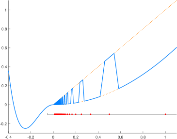
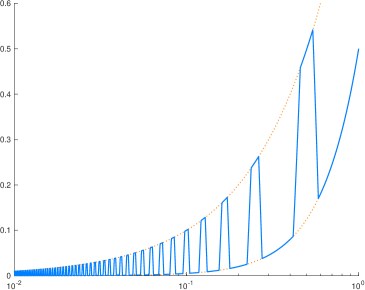
Figure 1: Plot of $f$. The function $f$ is depicted using a blue color. The dotted orange lines correspond to the functions $x\mapsto x$ and $x\mapsto\frac{1}{2}x^{2}$, respectively. The read points in subfigure (a) show the iterates $\bm{x}^{k}$, $k\in\mathbb{N}$. Subfigure (b) shows a logarithmic plot of $f$ on $[0.01,1]$.

Let $0\leq\nu<\kappa$ be given parameters. We consider the functions

$$~c(x):=\begin{cases}e^{-\frac{1}{x}}&\text{if }x>0,\\ 0&\text{otherwise},\end{cases}\quad\text{and}\quad\bar{c}_{\kappa,\nu}(x):=\frac{c(\kappa^{2}-x)}{c(\kappa^{2}-x)+c(x-\nu^{2})}.$$

The mappings $c$ and $\bar{c}_{\kappa,\nu}$ are obviously $C^{\infty}$ and we have $\bar{c}_{\kappa,\nu}(x)=0$ for all $x\geq\kappa^{2}$ and $\bar{c}_{\kappa,\nu}(x)=1$ for all $x\leq\nu^{2}$. Moreover, it holds that

$$c^{\prime}(x)=\begin{cases}\frac{1}{x^{2}}e^{-\frac{1}{x}}&\text{if }x>0,\\ 0&\text{otherwise},\end{cases}\quad\text{and}\quad\bar{c}^{\prime}_{\kappa,\nu}(x)=-\frac{c^{\prime}(\kappa^{2}-x)c(x-\nu^{2})+c(\kappa^{2}-x)c^{\prime}(x-\nu^{2})}{(c(\kappa^{2}-x)+c(x-\nu^{2}))^{2}}.$$

We now define $\kappa_{j}:=\frac{1}{4j(2j+1)}$, $\nu_{j}:=\frac{1}{8j(2j+1)}$, $g(x):=x-\frac{1}{2}x^{2}$, $\gamma_{j}(x):=g(x)\bar{c}_{\kappa_{j},\nu_{j}}((x-\frac{1}{2j})^{2})$, and

$$f(x):=\begin{cases}h(x)+\sum_{k=1}^{\infty}\gamma_{k}(x)&\text{if }x\neq 0,\\ ~0&\text{if }x=0,\end{cases}\quad\text{and}\quad h(x):=\begin{cases}\frac{1}{2}x^{2}&\text{if }x\geq 0,\\ 8x^{2}(8x^{2}-1)&\text{if }x<0.\end{cases}$$

An exemplary plot of the function $f$ is shown in Figure 1. The function $f$ is continuous on $\mathbb{R}$ and smooth for all $x\neq 0$. We now want to run gradient descent on $f$ with initial point $\bm{x}^{0}=1$ and diminishing step sizes

$$~\alpha_{k}:=\frac{1}{k+2},\;\;\text{if $k$ is even}\quad\text{and}\quad~\alpha_{k}:=\frac{1}{(k+1)(k+2)},\;\;\text{if $k$ is odd.}$$

Then, it follows

$$~\bm{x}^{k}=\frac{1}{k+1}\quad\text{and}\quad f^{\prime}(\bm{x}^{k})=\begin{cases}1&\text{if $k$ is even},\\ \frac{1}{k+1}&\text{if $k$ is odd}.\end{cases}$$ (39)

We now verify this statement by induction. We first notice that the functions $\{\gamma_{k}\}_{k\geq 0}$ and derivatives $\{\gamma_{k}^{\prime}\}_{k\geq 0}$ have disjoint supports $[\frac{1}{2k}-\frac{1}{4k(2k+1)},\frac{1}{2k}+\frac{1}{4k(2k+1)}]=[\frac{1}{2}(\frac{1}{2k}+\frac{1}{2k+1}),\frac{1}{2}(\frac{3}{2k}-\frac{1}{2k+1})]$ with center point $\frac{1}{2k}$, $k\in\mathbb{N}$. More specifically, we have

$$\gamma_{k}(x)=\begin{cases}0&\text{if }|x-\frac{1}{2k}|\geq\frac{1}{4k(2k+1)},\\ g(x)&\text{if }|x-\frac{1}{2k}|\leq\frac{1}{8k(2k+1)},\end{cases}\quad\text{and}\quad\gamma_{k}^{\prime}(x)=\begin{cases}0&\text{if }|x-\frac{1}{2k}|\geq\frac{1}{4k(2k+1)},\\ g^{\prime}(x)&\text{if }|x-\frac{1}{2k}|\leq\frac{1}{8k(2k+1)}.\end{cases}$$

Hence, (39) clearly holds for the base case $k=0$. Let us now assume that the induction hypothesis (39) is true for some $k$ and let $k+1=2j$, $j\in\mathbb{N}$, be an even number. Then, we obtain

$$\bm{x}^{k+1} =\bm{x}^{k}-\alpha_{k}f^{\prime}(\bm{x}^{k})$$

$$=\frac{1}{k+1}-\frac{1}{(k+1)(k+2)}\cdot\left[\frac{1}{k+1}+\gamma_{j}^{\prime}\left(\frac{1}{k+1}\right)\right]$$

$$=\frac{1}{k+1}-\frac{1}{(k+1)(k+2)}\cdot 1=\frac{1}{k+2}.$$

Similarly, if $k+1=2j+1$, $j\in\mathbb{N}$, is odd, we then have $\frac{1}{2j}-\frac{1}{k+1}=\frac{1}{2j(2j+1)}>\frac{1}{4j(2j+1)}$ and $\frac{1}{k+1}-\frac{1}{2j+2}=\frac{1}{(2j+1)(2j+2)}>\frac{1}{(2j+2)(2j+3)}$. This yields

$$~\bm{x}^{k+1}=\bm{x}^{k}-\alpha_{k}f^{\prime}(\bm{x}^{k})=\frac{1}{k+1}-\frac{1}{k+2}\cdot\frac{1}{k+1}=\frac{1}{k+2}.$$

This finishes the proof of (39). We further notice

$$~\sum_{k=0}^{\infty}\alpha_{k}\geq\sum_{k=0}^{\infty}\alpha_{2k}=\sum_{k=0}^{\infty}\frac{1}{2(k+1)}=\infty\quad\text{and}\quad\sum_{k=0}^{\infty}\alpha_{k}^{2}<\infty.$$

Consequently, the step sizes $\{\alpha_{k}\}_{k}$ satisfy all standard requirements. In addition, we have

$$\sum_{k=0}^{\infty}\alpha_{k}|f^{\prime}(\bm{x}^{k})|^{2}\leq\sum_{k=0}^{\infty}\frac{1}{(k+1)(k+2)}<\infty\quad\text{and}\quad\min_{k=0,\dots,T}|f^{\prime}(\bm{x}^{k})|^{2}\leq\frac{1}{T^{2}}.$$

Thus, the complexity results in (38) obviously hold, but the gradient values $f^{\prime}(\bm{x}^{k})$ do not converge to zero. In particular, for even $T$, the last iterate $\bm{x}^{T}$ satisfies $f^{\prime}(\bm{x}^{T})=1$ which obstructs interpretability of $\bm{x}^{T}$ and of the complexity bounds $\min_{k=0,\dots,T}|f^{\prime}(\bm{x}^{k})|^{2}\leq\varepsilon$ or $|f^{\prime}(\bm{x}^{\bar{k}})|^{2}\leq\varepsilon$. Notice that the mapping $f$ is not Lipschitz smooth around $x=0$ and hence, the convergence results in 2.1 are not applicable here. Of course, these observations have even higher significance in the stochastic setting, when evaluation of the bounds (37) is generally restrictive or not possible within the algorithmic procedure.

We conclude and summarize our discussion with a comment by Francesco Orabona on non-asymptotic and asymptotic convergence analyses for $\mathsf{SGD}$ ([32], blog post: “Almost sure convergence of SGD on smooth non-convex functions”, section 5 and 6, Oct. 05, 2020):

References

- [1] Yves F. Atchadé, Gersende Fort, and Eric Moulines. On perturbed proximal gradient algorithms. J. Mach. Learn. Res., 18(10):1–33, 2017.
- [2] Amir Beck. First-order methods in optimization. SIAM, Philadelphia, PA, 2017.
- [3] Dimitri P. Bertsekas and John N. Tsitsiklis. Gradient convergence in gradient methods with errors. SIAM J. Optim., 10(3):627–642, 2000.
- [4] Axel Böhm and Stephen J. Wright. Variable smoothing for weakly convex composite functions. J. Optim. Theory Appl., 188(3):628–649, 2021.
- [5] Léon Bottou. Stochastic learning. In Summer School on Machine Learning, pages 146–168. Springer, 2003.
- [6] Léon Bottou, Frank E. Curtis, and Jorge Nocedal. Optimization methods for large-scale machine learning. SIAM Review, 60(2):223–311, 2018.
- [7] Leo Breiman. Probability, volume 7 of Classics in Applied Mathematics. Society for Industrial and Applied Mathematics (SIAM), Philadelphia, PA, 1992. Corrected reprint of the 1968 original.
- [8] Andrew R. Conn, Nicholas I. M. Gould, and Philippe L. Toint. Trust-region methods. MPS/SIAM Series on Optim. SIAM; MPS, Philadelphia, PA, 2000.
- [9] J-C Culioli and Guy Cohen. Decomposition/coordination algorithms in stochastic optimization. SIAM J. Control Optim., 28(6):1372–1403, 1990.
- [10] Damek Davis and Dmitriy Drusvyatskiy. Stochastic model-based minimization of weakly convex functions. SIAM J. Optim., 29(1):207–239, 2019.
- [11] Damek Davis, Dmitriy Drusvyatskiy, Sham Kakade, and Jason D. Lee. Stochastic subgradient method converges on tame functions. Found. Comput. Math., 20(1):119–154, 2020.
- [12] Dmitriy Drusvyatskiy and Adrian S. Lewis. Error bounds, quadratic growth, and linear convergence of proximal methods. Math. Oper. Res., 43(3):919–948, 2018.
- [13] John C. Duchi and Feng Ruan. Stochastic methods for composite and weakly convex optimization problems. SIAM J. Optim., 28(4):3229–3259, 2018.
- [14] Jianqing Fan. Comments on “wavelets in statistics: A review” by A. Antoniadis. Journal of the Italian Statistical Society, 6(2):131, 1997.
- [15] Caroline Geiersbach and Teresa Scarinci. Stochastic proximal gradient methods for nonconvex problems in Hilbert spaces. Comput. Optim. Appl., 78(3):705–740, 2021.
- [16] Saeed Ghadimi and Guanghui Lan. Stochastic first-and zeroth-order methods for nonconvex stochastic programming. SIAM J. Optim., 23(4):2341–2368, 2013.
- [17] Saeed Ghadimi, Guanghui Lan, and Hongchao Zhang. Mini-batch stochastic approximation methods for nonconvex stochastic composite optimization. Math. Program., 155(1-2, Ser. A):267–305, 2016.
- [18] Robert Gower, Othmane Sebbouh, and Nicolas Loizou. SGD for structured nonconvex functions: Learning rates, minibatching and interpolation. In Proceedings of The 24th International Conference on Artificial Intelligence and Statistics, volume 130, pages 1315–1323. PMLR, 13–15 Apr 2021.
- [19] Mert Gürbüzbalaban, Asu Ozdaglar, and P. A. Parrilo. Why random reshuffling beats stochastic gradient descent. Math. Program., 186(1-2):49–84, 2021.
- [20] Tim Hoheisel, Maxime Laborde, and Adam Oberman. A regularization interpretation of the proximal point method for weakly convex functions. J. Dyn. Games, 7(1):79–96, 2020.
- [21] Ya-Ping Hsieh, Panayotis Mertikopoulos, and Volkan Cevher. The limits of min-max optimization algorithms: Convergence to spurious non-critical sets. In International Conference on Machine Learning, pages 4337–4348. PMLR, 2021.
- [22] Ahmed Khaled and Peter Richtárik. Better theory for SGD in the nonconvex world. arXiv preprint, arXiv:2002.03329, 2020.
- [23] Yunwen Lei, Ting Hu, Guiying Li, and Ke Tang. Stochastic gradient descent for nonconvex learning without bounded gradient assumptions. IEEE Transactions on Neural Networks and Learning Systems, 31(10):4394–4400, 2019.
- [24] Xiao Li, Andre Milzarek, and Junwen Qiu. Convergence of random reshuffling under the Kurdyka-Łojasiewicz inequality. arXiv preprint, arXiv:2110.04926, 2021.
- [25] Xiaoyu Li and Francesco Orabona. On the convergence of stochastic gradient descent with adaptive stepsizes. In The 22nd International Conference on Artificial Intelligence and Statistics, pages 983–992. PMLR, 2019.
- [26] Szymon Majewski, Blazej Miasojedow, and Eric Moulines. Analysis of nonsmooth stochastic approximation: the differential inclusion approach. arXiv preprint, arXiv:1805.01916v1, 2018.
- [27] Panayotis Mertikopoulos, Nadav Hallak, Ali Kavis, and Volkan Cevher. On the almost sure convergence of stochastic gradient descent in non-convex problems. Advances in Neural Information Processing Systems, 33:1117–1128, 2020.
- [28] Andre Milzarek, Fabian Schaipp, and Michael Ulbrich. A semismooth Newton stochastic proximal point algorithm with variance reduction. arXiv preprint, arXiv:2204.00406v1, 2022.
- [29] Konstantin Mishchenko, Ahmed Khaled, and Peter Richtárik. Random reshuffling: Simple analysis with vast improvements. Advances in Neural Information Processing Systems, 33:17309–17320, 2020.
- [30] Yu. Nesterov. Gradient methods for minimizing composite functions. Math. Program., 140(1, Ser. B):125–161, 2013.
- [31] Lam M Nguyen, Quoc Tran-Dinh, Dzung T Phan, Phuong Ha Nguyen, and Marten van Dijk. A unified convergence analysis for shuffling-type gradient methods. J. Mach. Learn., 22(207):1–44, 2021.
- [32] Francesco Orabona. Almost sure convergence of SGD on smooth non-convex functions. https://parameterfree.com/2020/10/05/almost-sure-convergence- of-sgd-on-smooth-non-convex-functions/, 2020.
- [33] Boris T Polyak and Anatoli B Juditsky. Acceleration of stochastic approximation by averaging. SIAM J. Control Optim., 30(4):838–855, 1992.
- [34] Sashank. J. Reddi, Suvrit Sra, Barnabas Póczos, and Alexander J Smola. Proximal stochastic methods for nonsmooth nonconvex finite-sum optimization. In Advances in Neural Information Processing Systems 29, pages 1145–1153. Curran Associates, Inc., 2016.
- [35] Herbert Robbins and Sutton Monro. A stochastic approximation method. The Annals of Mathematical Statistics, pages 400–407, 1951.
- [36] Herbert Robbins and David Siegmund. A convergence theorem for non negative almost supermartingales and some applications. In Optimizing Methods in Statistics, pages 233–257. Elsevier, 1971.
- [37] R. Tyrrell Rockafellar. Convex analysis. Princeton Landmarks in Mathematics. Princeton University Press, Princeton, NJ, 1997. Reprint of the 1970 original, Princeton Paperbacks.
- [38] R. Tyrrell Rockafellar and Roger J.-B. Wets. Variational analysis, volume 317 of Grundlehren der mathematischen Wissenschaften [Fundamental Principles of Mathematical Sciences]. Springer-Verlag, Berlin, 1998.
- [39] Lorenzo Rosasco, Silvia Villa, and B. Công Vũ. Convergence of stochastic proximal gradient algorithm. Appl. Math. Optim., 82(3):891–917, 2020.
- [40] Othmane Sebbouh, Robert M Gower, and Aaron Defazio. Almost sure convergence rates for stochastic gradient descent and stochastic heavy ball. In Conference on Learning Theory, pages 3935–3971. PMLR, 2021.
- [41] Ohad Shamir and Tong Zhang. Stochastic gradient descent for non-smooth optimization: Convergence results and optimal averaging schemes. In International Conference on Machine Learning, pages 71–79. PMLR, 2013.
- [42] Daniel W. Stroock. Probability theory. Cambridge University Press, Cambridge, second edition, 2011. An analytic view.
- [43] Jean-Philippe Vial. Strong and weak convexity of sets and functions. Math. Oper. Res., 8(2):231–259, 1983.
- [44] Cun-Hui Zhang. Nearly unbiased variable selection under minimax concave penalty. Ann. Statist., 38(2):894–942, 2010.
- [45] Tong Zhang. Solving large scale linear prediction problems using stochastic gradient descent algorithms. In Proceedings of the Twenty-First International Conference on Machine Learning, page 116, 2004.