Search efficiency in the Adam-Delbrück reduction-of-dimensionality scenario versus direct diffusive search

Abstract

The time instant—the first-passage time (FPT)—when a diffusive particle (e.g., a ligand such as oxygen or a signalling protein) for the first time reaches an immobile target located on the surface of a bounded three-dimensional domain (e.g., a hemoglobin molecule or the cellular nucleus) is a decisive characteristic time-scale in diverse biophysical and biochemical processes, as well as in intermediate stages of various inter- and intra-cellular signal transduction pathways. Adam and Delbrück put forth the reduction-of-dimensionality concept, according to which a ligand first binds non-specifically to any point of the surface on which the target is placed and then diffuses along this surface until it locates the target. In this work, we analyse the efficiency of such a scenario and confront it with the efficiency of a direct search process, in which the target is approached directly from the bulk and not aided by surface diffusion. We consider two situations: (i) a single ligand is launched from a fixed or a random position and searches for the target, and (ii) the case of "amplified" signals when $N$ ligands start either from the same point or from random positions, and the search terminates when the fastest of them arrives to the target. For such settings, we go beyond the conventional analyses, which compare only the mean values of the corresponding FPTs. Instead, we calculate the full probability density function of FPTs for both scenarios and study its integral characteristic—the "survival" probability of a target up to time $t$. On this basis, we examine how the efficiencies of both scenarios are controlled by a variety of parameters and single out realistic conditions in which the reduction-of-dimensionality scenario outperforms the direct search.
Keywords: Ligand binding to a target site, first-passage times, probability density functions, Adam-Delbrück reduction-of-dimensionality scenario, bulk and surface diffusion

1 Introduction

More than five decades ago Adam and Delbrück put forth an idea how organisms may handle some problems of efficiency and timing, limited by molecular diffusion, by reducing the dimensionality in which the diffusion takes place from the three-dimensional (bulk) space to two-dimensional surface diffusion [1]. A similar claim was previously made in [2], suggesting that acetyl choline may get faster via surface diffusion from its site of action to the site where it is destroyed, and in [3], arguing that surface diffusion may result in higher turnover numbers for membrane-bound enzymes. However, these earlier works did not present quantitative estimates substantiating such a claim, while Adam and Delbrück were the first to provide theoretical arguments showing that the diffusive molecules may indeed reduce the reaction times by subdividing the diffusion process into successive stages of lower spatial dimensionality. Subsequently, their analysis has been generalised in a number of directions (see, e.g., [4, 5, 6, 7, 8, 9, 10, 11, 12, 13]). Its applicability has also been questioned [14], indicating situations in which the "reduction-of-dimensionality" scenario can be advantageous and therefore plausible, and situations in which it is not beneficial for the search process and is therefore not likely to occur.

Concurrently, the concept of a dimensionality reduction together with the notion of "facilitated" diffusion provide an explanation why experimentally observed rates for binding of proteins to special sites on DNA molecules are much larger than predictions based on the Smoluchowski approach [5, 15, 16, 17, 18, 19, 20, 21, 22, 23, 24, 26, 27, 25, 28, 29]. The Adam-Delbrück scenario (ADS) was also invoked to explain a fast translocation through the nuclear pore complexes [30]. This scenario also prompted further investigations giving rise to the idea of so-called intermittent search strategies [31, 32] in which the fine tuning of systems parameters may further reduce the mean first-passage time [33, 34, 37, 35, 36, 38, 39, 40] (see however [41]) or the "survival" probability—the probability that the target is not found up to time $t$ [42, 43, 44] (in transient processes it is also of interest to consider the search reliability, the probability that the target has not been found up to $t\to\infty$ [45, 46]).

To better illustrate the possible advantage of the ADS, it is instructive to dwell on a particular geometrical setting, which was discussed by Adam and Delbrück themselves [1] and will be also used in the present paper. Namely, we consider two nested concentric spheres (of radii $R_{1}$ and $R_{2}$ ($R_{1}<R_{2}$), respectively, as shown in figure 1) with impermeable boundaries, a small immobile circular target of radius $\rho$ placed at some fixed position on the inner sphere, and a ligand that starts from a fixed location and diffuses with the diffusion coefficient $D_{b}$ within the spherical-shell domain $\Omega$ between two spheres (here and in what follows we use the term "ligand" to denote any diffusing entity, e.g., a signalling protein; similarly, the term "target" will generally denote a binding site, an adsorbed chemically active particle or an entrance to a nuclear pore). In such a bounded domain, a ligand is certain to eventually find the target (see, e.g. [47]), whichever motion scenario it undertakes—and therefore the only question is how long the search process will last for a given scenario. We therefore are interested in the first-passage time (FPT) $\mathcal{T}$, i.e., a random time instant when a ligand reaches the target for the first time (see, e.g., [48, 49]).

Conventional one-stage (or direct search) scenario presumes that the inner sphere is reflecting for the ligand such that it bounces back to the bulk domain $\Omega$ once it hits the inner sphere everywhere except for the target. The binding event thus occurs only when the target is approached by the ligand directly from the bulk. Assuming that the starting position of the ligand is uniformly distributed within the spherical-shell domain, Adam and Delbrück [1] (see also [7]) estimated the mean "diffusion" time $\tau_{\rm dir}$ necessary for the ligand to arrive to the target within the one-stage scenario as $\tau_{\rm dir}\sim R_{2}^{3}/(3D_{b}\rho)$ (in the relevant case when $R_{2}\gg R_{1}\gg\rho$). In fact, $\tau_{\rm dir}$ here is the mean diffusion time to a sphere of radius $\rho$ placed at the geometric centre of the outer sphere and thus this form does not take into account the fact that the target is situated on a reflecting sphere of radius $R_{1}$, which effectively screens it [50]. Moreover, for a relevant geometrical setting in which the ligand starts from the outer sphere, $\tau_{\rm dir}$ will be evidently bigger. Not least, this reasoning clearly applies only to an idealised situation when the confining domain $\Omega$ does not contain "obstacles" and the motion of the ligand is not subject to any kind of molecular crowding effects [51, 52]. However, if $\Omega$ is supposed to mimic the interior of a cell, it should represent a complex spatial environment, filled with impermeable organelles, filaments and proteins, which impose steric constraints on the dynamics and may screen the target. As a consequence, diffusion of a ligand often takes place effectively in a tortuous labyrinthine spatial domain. Recent analyses have provided evidence that the FPT to the target within the direct search scenario is essentially increased as compared to the one in which the cytosol is treated as a homogeneous liquid-filled region [53]. Hence, the above estimate can be rather inaccurate (in fact, representing a lower bound on the actual diffusion time) but is still instructive for understanding the time scales involved.

In contrast, within the ADS a ligand first finds any (random) point on the inner sphere, which takes the typical time $\tau_{b}\sim R_{2}^{3}/(3D_{b}R_{1})$. Then, it nonspecifically binds to the surface and diffuses along with the diffusion coefficient $D_{s}$ until it eventually locates the target. The mean diffusion time $\tau_{s}$ for the latter process was calculated [1, 7] and scales as $\tau_{s}\sim 2R_{1}^{2}\ln(R_{1}/\rho)/D_{s}$. The total mean diffusion time $\tau_{\rm AD}$ within the ADS is thus a sum of two contributions, $\tau_{\rm AD}=\tau_{b}+\tau_{s}$, and the ratio

$$\delta=\frac{\tau_{\rm AD}}{\tau_{\rm dir}}=\frac{\rho}{R_{1}}\left(1+6\frac{D_{b}}{D_{s}}\left(\frac{R_{1}}{R_{2}}\right)^{3}\ln\left(\frac{R_{1}}{\rho}\right)\right)$$ (1)

shows whether the reduction-of-dimensionality scenario is advantageous (for $\delta<1$) or not. One observes from equation (1) that the efficiency of the ADS here is entirely controlled by the aspect ratios $\rho/R_{1}$ and $R_{1}/R_{2}$ and the ratio $D_{s}/D_{b}$ of the diffusion coefficients. Clearly, $\tau_{b}$ can also be larger, when obstacles are present in the bulk volume $\Omega$ but intuitively, its increase should not be as pronounced as the one for the direct search of the target—within the ADS it suffices to find any point on the inner sphere while for the direct search scenario a prescribed target location is to be found.

In essence, the ADS takes advantage of the very slow logarithmic divergence of $\tau_{\rm AD}$ in the limit $\rho\to 0$, as opposed to a much faster $1/\rho$-divergence of $\tau_{\rm dir}$ for the direct search scenario. At the same time, there is a penalty to pay: the gain due to the reduction of the singularity is counter-balanced by the reduction of the value of the diffusion coefficient. For instance, the diffusion coefficient $D_{b}$ of a ligand in cellular cytoplasm is typically of the order of a few tens of $\mu\mathrm{m}^{2}/\mathrm{s}$, while once it gets associated to the inner sphere, it experiences at best a $20$-fold reduction of the diffusivity [13]. Most often, however, such a reduction is more pronounced and may amount to two or sometimes even three orders of magnitude [14]. Such an extreme reduction is, however, rarely seen in biophysical systems because most of compartment-separating surfaces are soft and hence, the barriers against lateral diffusion are typically lower than the ones specific to diffusion on hard solid surfaces [55]. In any case, a reduction of the diffusivity is detrimental for the ADS, in virtue of equation (1). As an example, consider a typical mammalian cell in which a class I nuclear receptor searches for an entrance into a pore (of radius $\rho\sim 3{\rm nm}$) in the nuclear envelope. For eukaryotes, the karyoplasmic ratio (KR) typically is of the order $(R_{1}/R_{2})^{3}\sim 0.08$ (see, e.g., [56]), but the scatter around this value can be quite significant. In particular, essential departures from the value $0.08$ are encountered in metastatic tumours and are, in fact, used in both diagnosis and prognosis for several tumour types [57]. Recent systematic analysis [58] of the reported values of the KR, which compiled data for almost $900$ species—from yeast to mammals—provided evidence that the larger cells almost invariably have relatively smaller nuclei, such that the nucleus of a larger cell may occupy as little as few percent of the cell volume across all scales of biological organisation, yielding lower values of KR. For plant cells, which can often grow to larger sizes than animal cells, it has been known for a long time that KR can be even smaller and amount to just a fraction of $1$ percent (see, e.g., Table I in [59]). Concurrently, $R_{1}$ may vary in size in different species but is usually within the range $1\ldots 5\mu\mathrm{m}$. Setting $R_{1}=3\mu\mathrm{m}$ and $\rho=3{\rm nm}$ and assuming that KR is equal to its average value $0.08$, i.e., $R_{2}=7\mu\mathrm{m}$, we thus find $\delta=3.4\times 10^{-3}D_{b}/D_{s}$, which signifies that for these particular values of the system parameters the ADS is advantageous when $D_{s}/D_{b}\gtrsim 10^{-2}$. For larger cells or some plant cells, for which KR is lower, and also in situations in which the direct search for the entrance to the nuclear pore is obstructed by the presence of other organelles, one may expect that the ADS is efficient even for smaller values of the ratio $D_{s}/D_{b}$.

The above well-known arguments rely on estimates of the mean FPT (MFPT), used as a proxy for the efficiency. In this work we revisit the ADS from the broader perspective of the full statistics of FPTs. The point is that, regardless of how a search process proceeds—via a single or two stages—a ligand may follow a variety of different paths from the starting point to the target, thus resulting in a large variability of realisation-dependent values of the FPT. The mean FPT, which is only the first moment of the corresponding probability density function (PDF) averaged over the initial position of the ligand, is instructive—yet it is evidently insufficient to fully characterise neither the ADS nor the direct search scenario. In fact, it is well-known that for bulk diffusion in a bounded confining domain towards a perfect sink (see, e.g., [60, 61, 62, 63]), or a partially reactive target (see, e.g., [64, 65, 66]), or even a target with more sophisticated surface reaction mechanism (see, e.g., [67, 68, 69]), the PDF of the FPTs can be very broad. In other words, large sample-to-sample fluctuations with disproportionally different values of $\mathcal{T}$ are inherent and fluctuations around its mean value $\langle\mathcal{T}\rangle$ can be comparable to it or even exceed the mean value. It is known from standard statistical analysis that if the PDF is centred around its mean value (e.g., in the case of a Gaussian distribution), the mean value is representative of the actual behaviour. In contradistinction, if the mean is well away from the most probable value (as shown, e.g., in [64, 65, 66, 62, 63]) it is likely that it is associated with the tail of the corresponding PDF and hence, is supported by some rare realisations of the diffusive paths. In this case, $\langle\mathcal{T}\rangle$ may be orders of magnitude larger than the typical time encountered in a considerable fraction of realisations of the search process (and thus times shorter than the mean time are typically observed in any given experiment). This would also imply that one indeed needs an extensive statistical sample in order to obtain a reliable value for $\langle\mathcal{T}\rangle$ for comparison with theoretical predictions. This is precisely the case for the direct search scenario in such a geometrical setting, as evidenced recently in [50]. Concurrently, the full PDF of the FPT for the two-stage search process is not known as yet and consequently, one does not know anything about its broadness and other characteristic time scales (e.g., the typical FPT), that is indispensable in order to obtain a fully comprehensive, global picture of the search dynamics in the ADS. The knowledge of the full PDF will also permit us to use as a robust characteristic the survival probability, i.e., the probability that the target is not found up to some prescribed time $t$.

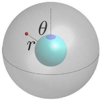
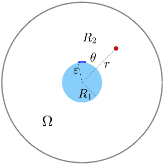
Figure 1: Sketch of the geometrical setup in the study of the ADS: a spherical shell domain $\Omega$ is enclosed by impermeable boundaries consisting of two concentric nested spheres with the radii $R_{1}$ (the inner sphere) and $R_{2}$ (the outer, fully reflective sphere). A target region is located at the North pole of the inner sphere and has the form of a spherical cap of radius $\rho$ (and angular size $\varepsilon=\arcsin(\rho/R_{1})$). A small red ball denotes the starting position $\mathbf{x}=(r,\theta,\phi)$ of the diffusive ligand. Within the ADS, the ligand diffuses (with diffusion coefficient $D_{b}$) within $\Omega$ until it encounters the surface of the inner sphere, which happens at an arbitrary point $\mathbf{s}=(R_{1},\theta^{\prime},\phi^{\prime})$. Then, it non-specifically binds to the surface and diffuses along it with diffusion coefficient $D_{s}$, until it finds the boundary of the target region. Within the direct search scenario, the surface of the inner sphere is assumed to be perfectly reflecting such that the ligand bounces back to $\Omega$ once it hits the inner sphere and may reach the target region only directly from the bulk $\Omega$.

In this paper, we first consider the case of a single ligand starting from an arbitrary fixed position within the spherical-shell domain $\Omega$ and a single perfect target placed on the inner sphere. The term "perfect" here means that we assume that there is no (energetic or entropic) barrier against the reaction, such that the ligand binds to the target upon the first arrival—the classical Smoluchowski setting. In the ADS, we calculate the PDF of the FPTs to the target exactly, which permits us to analyse the spread of the realisation-dependent FPTs, as well as to understand the contribution of the typical first-passage time and of extreme events associated with the tails of the distribution. Moreover, we compare our result against the PDF for the direct search scenario, which was evaluated for the same geometrical setting recently [50], in an exact spectral form as well as in approximate but remarkably accurate form based on the self-consistent approximation (see [10, 70, 71, 72] for more details). Such a comparison between the ADS and a one-stage search under identical conditions allows us to provide a complete picture of the actual efficiency of the ADS which extends beyond the previous analyses. Next, we consider the situation with an "amplified signal", in which $N$ ligands are launched either from the same location on the outer sphere, or from distinct locations on this surface. The former case is realised in situations when some other ligand (e.g., a first messenger), which is moving diffusively in the extracellular medium, arrives to a particular site on the outer part of the plasma membrane and opens an ion channel spanning the membrane. In this way, the first messenger effects $N$ ions to release inside the cell from the same position. In turn, the latter case corresponds to a situation when the plasma membrane hosts multiple receptors each interacting with the first messengers moving in the extracellular medium and launching the second messengers that diffuse now within the intracellular medium, all of them seeking a single target on the inner sphere [73, 74]. For such amplified signals we also provide a comparative analysis of the PDFs for the one-stage and two-stages scenarios. We finally remark that the results presented here can be generalised rather straightforwardly for the analysis of the PDFs of the terminal FPT in intracellular signal transduction processes involving more than two nested domains (see [75]), presenting in this way a full stochastic description of the latter important processes within the reduction-of-dimensionality scenario.

The paper is outlined as follows: In section 2, we describe the geometrical and physical parameters of our model, introduce basic notations, and derive the PDF of the first-passage times within the ADS. Section 3 is devoted to the analysis of our general result and of its asymptotic behaviour, and also presents a comparison of the form of the PDF for the ADS against the results for the direct, one-stage scenario derived in [50]. In section 4 we consider the situation of an amplified signal with $N$ independent ligands. Finally, in section 5 we conclude with a brief recapitulation of our results and a discussion. Details of intermediate derivations, as well as an analysis of some limiting situations are relegated to Appendices. In particular, A considers the moments of the conditioned first-passage times; B is devoted to a discussion of different aspects of extremal values of surface diffusion; in C we discuss the form of the PDF for the Adam-Delbrück’s scenario, while in D we present the PDF for one-stage search process.

2 The ADS in a spherical shell domain

2.1 Model and basic notations

We consider a spherical shell domain $\Omega$ (see figure 1) enclosed by impermeable boundaries of two concentric nested spheres with radii $R_{1}$ (the inner sphere) and $R_{2}$ (the outer, perfectly reflecting sphere). An immobile target with the shape of a spherical cap (dome) of radius $\rho$ is located at the North pole of the inner sphere. In spherical coordinates $(r,\theta,\phi)$, the target is defined by $r=R_{1}$ and $0\leq\theta\leq\varepsilon$, where $\varepsilon=\arcsin(\rho/R_{1})$ is the angular size of the target. For the above example of a nuclear receptor seeking for a nuclear pore (as well as in many other realistic cases) $\varepsilon\approx 10^{-3}$, but the value may be smaller or larger in other applications. We note parenthetically that values $\varepsilon\approx 10^{-1}$ can be indicative of the behaviour in situations when there are many small targets present on the surface of the inner sphere (e.g., the nuclear membrane may host about $10^{2}$ nuclear pores). As a consequence, we here consider $\varepsilon$ as an independent parameter and explore the dependence of the PDFs on its value. Moreover, we also consider the ratio $D_{b}/D_{s}$ as an independent parameter and analyse how the shape of the PDF itself along with the survival probability vary with this ratio.

2.2 General expressions

Consider now a ligand that starts from a fixed position $\mathbf{x}$, performs a diffusive motion with bulk diffusivity $D_{b}$ inside the spherical-shell domain, until it hits the inner sphere for the first time at the random time $\mathcal{T}^{\rm bulk}$. Then, it diffuses along the surface for the random time $\mathcal{T}^{\rm surf}$ after which the ligand hits the perimeter of the target for the first time. The fact that the search process consists of two consecutive independent stages of durations $\mathcal{T}^{\rm bulk}$ and $\mathcal{T}^{\rm surf}$ permits us to write the PDF $H^{\rm AD}(t;\mathbf{x})$ of the event that it took the ligand exactly time $\mathcal{T}=\mathcal{T}^{\rm bulk}+\mathcal{T}^{\rm surf}$ to arrive to the target for the first time as the convolution

$$H^{\rm AD}(t;\mathbf{x})=\int_{\partial\Omega}d\mathbf{s}\int^{t}_{0}dt_{1}\,H^{\rm surf}(t-t_{1};\mathbf{s})\,j(t_{1};\mathbf{s}|\mathbf{x}),$$ (2)

where the first integral over $d\mathbf{s}$ is taken over the surface $\partial\Omega$ of the inner sphere. Here $j(t_{1};\mathbf{s}|\mathbf{x})$ denotes the joint PDF of the event that a ligand starting from $\mathbf{x}$ at time $t=0$ arrived for the first time at the inner sphere at time $t_{1}$ and that this first arrival occurred at point $\mathbf{s}$. In turn, $H^{\rm surf}(t_{2}|\mathbf{s})$ denotes the PDF that the duration of the surface diffusion, starting from the point $\mathbf{s}$ and terminating when the ligand arrives at any point on the perimeter of the target, is equal to $t_{2}$. An analogous expression for more general $n$-stage processes in one-, two- and three-dimensional unbounded domains has been recently studied in [75].

The form of expression (2) suggests that it can be conveniently studied by resorting to the Laplace domain with respect to $t$. Let

$$\tilde{H}^{\rm AD}(p;\mathbf{x})=\int^{\infty}_{0}dt\,e^{-pt}\,H^{\rm AD}(t;\mathbf{x}),\qquad\tilde{H}^{\rm surf}(p;\mathbf{s})=\int^{\infty}_{0}dt\,e^{-pt}H^{\rm surf}(t;\mathbf{s})$$ (3)

and

$$\tilde{j}(p;\mathbf{s}|\mathbf{x})=\int^{\infty}_{0}dt\,e^{-pt}\,j(t;\mathbf{s}|\mathbf{x})$$ (4)

denote the Laplace-transformed PDFs. Then, multiplying both sides of equation (2) by $\exp(-pt)$ and taking the integral, we find

$$\tilde{H}^{\rm AD}(p;\mathbf{x}) =\int_{\partial\Omega}d\mathbf{s}\,\tilde{H}^{\rm surf}(p;\mathbf{s})\,\tilde{j}(p;\mathbf{s}|\mathbf{x})$$

$$=R_{1}^{2}\int\limits_{0}^{\pi}d\theta^{\prime}\,\sin\theta^{\prime}\int\limits_{0}^{2\pi}d\phi^{\prime}\,\tilde{j}(p,(R_{1},\theta^{\prime},\phi^{\prime})|(r,\theta,\phi))\,\tilde{H}^{\rm surf}(p;\theta^{\prime}),$$ (5)

where the spherical coordinates $\theta^{\prime}$ and $\phi^{\prime}$ define the position of the point $\mathbf{s}$, at which the ligand first lands on the inner sphere, while the coordinates $(r,\theta,\phi)$ denote the position of the starting point $\mathbf{x}$. Note that due to the axial symmetry, $\tilde{H}^{\rm surf}(p;\theta^{\prime})$ is independent of the azimuthal angle $\phi^{\prime}$.

Equation (2.2) is the basis for our further analysis, but it requires knowledge of the corresponding FPTs of the intermediate stages. The exact form of $\tilde{j}(p;\mathbf{x}|\mathbf{s})$ has been recently studied in [76] and obeys

$$\tilde{j}(p,\mathbf{s}|\mathbf{x})=\frac{1}{4\pi R_{1}^{2}}\sum\limits_{n=0}^{\infty}(2n+1)P_{n}\left(\frac{(\mathbf{s}\cdot\mathbf{x})}{|\mathbf{s}||\mathbf{x}|}\right)g_{n}^{(p)}(r),$$ (6)

where

$$g_{n}^{(p)}(r)=\frac{k^{\prime}_{n}(\alpha R_{2})i_{n}(\alpha r)-i^{\prime}_{n}(\alpha R_{2})k_{n}(\alpha r)}{k^{\prime}_{n}(\alpha R_{2})i_{n}(\alpha R_{1})-i^{\prime}_{n}(\alpha R_{2})k_{n}(\alpha R_{1})}$$ (7)

are the radial functions, $\alpha=\sqrt{p/D_{b}}$, $i_{n}(z)=\sqrt{\pi/(2z)}I_{n+1/2}(z)$, and $k_{n}(z)=\sqrt{2/(\pi z)}\,K_{n+1/2}(z)$ are the modified spherical Bessel functions of the first and second kind, respectively. The prime denotes a derivative with respect to the argument, and $P_{n}(z)$ are Legendre polynomials whose argument is the cosine of the angle between the vectors $\mathbf{x}$ and $\mathbf{s}$. In particular, equation (6) defines the moments of the FPT on the inner sphere, conditioned by the arrival point $\mathbf{s}$ (see A).

The above expression for $\tilde{j}(p,\mathbf{s}|\mathbf{x})$ is valid even in the limit $R_{2}\to\infty$ (e.g., when $R_{2}$ becomes macroscopically large, as is often the case in cell-to-cell communication processes) when the outer reflecting boundary practically goes to infinity and one retrieves a common setting of a spherical target, accessed by a particle diffusing in the unbounded space $\Omega$. Even though the domain itself is unbounded, its boundary ${\partial\Omega}$ is bounded, and the above solution is still applicable. From the asymptotic behaviour of the modified spherical Bessel functions $i_{n}(z)$ and $k_{n}(z)$, one gets immediately that the radial functions $g_{n}^{(p)}(r)$ converge to

$$g_{n}^{(p)}(r)\to\frac{k_{n}(\alpha r)}{k_{n}(\alpha R_{1})}.$$ (8)

In the following, we keep focusing on the setting with a finite $R_{2}$.

2.3 Surface diffusion stage

Despite the fact that the first-passage statistics for a particle diffusing on the surface of a spherical domain toward a target of an arbitrary size has been studied in the past, former works focused mostly on the MFPT [1, 7] (see also [77, 78, 79, 80] and references therein). Notable exceptions are the Refs. [77, 78], in which the spectral expansion of the survival probability in time domain was derived. While its Laplace transform allows one to access $\tilde{H}^{\rm surf}(p;\mathbf{s})$ as a spectral expansion, as well, we get a more compact form for this function that is suitable for further analysis of $\tilde{H}^{\rm AD}(p;\mathbf{x})$ in equation (2.2). Relegating the details of calculations to B below we merely display the final results for $\tilde{H}^{\rm surf}(p;\mathbf{s})$ and $H^{\rm surf}(t;\mathbf{s})$. When diffusion starts within the target, one has

$$\tilde{H}^{\rm surf}(p;\theta^{\prime})=1\quad(0\leq\theta^{\prime}\leq\varepsilon);$$ (9)

in turn, for $\varepsilon\leq\theta^{\prime}\leq\pi$, one gets the remarkably compact form

$$\tilde{H}^{\rm surf}(p;\theta^{\prime})=\frac{P_{\mu}(-\cos(\theta^{\prime}))}{P_{\mu}(-\cos(\varepsilon))},\qquad\mu=\frac{-1+\sqrt{1-4pR_{1}^{2}/D_{s}}}{2},$$ (10)

where $P_{\mu}(z)$ is the Legendre function of order $\mu$ which depends on the Laplace parameter $p$. Note that for $p\ll D_{s}/(4R_{1}^{2})$ (corresponding to the long-$t$ tail of the PDF), the parameter $\mu$ is a real number, while in the opposite limit $p\gg D_{s}/(4R^{2}_{1})$ (corresponding to the short-$t$ tail of the PDF), $\mu$ is a complex number with a real part equal to $-1/2$, such that $P_{\mu}(z)$ is related to the so-called conical (or Mehler) function. Expression (10) can be inverted (see B for more details) to produce the spectral expansion (see also [77, 78])

$$H^{\rm surf}(t;\theta^{\prime}) =\frac{D_{s}\sin^{2}(\varepsilon)}{R_{1}^{2}}\sum_{n=0}^{\infty}\left(\int^{1}_{-\cos(\varepsilon)}dx\left[P_{\nu_{n}}(x)\right]^{2}\right)^{-1/2}P_{\nu_{n}}(-\cos(\theta^{\prime}))P^{\prime}_{\nu_{n}}(-\cos(\varepsilon))$$

$$\qquad\times e^{-\nu_{n}(\nu_{n}+1)D_{s}t/R^{2}_{1}},$$ (11)

where the prime, as in equation (7), denotes the derivative with respect to the argument, while $\nu_{n}$ are the solutions of

$$P_{\nu_{n}}(-\cos(\varepsilon))=0$$ (12)

organised in an ascending order. Evidently, $\nu_{n}$ are functions of $\varepsilon$. Eventually, we note that the moments of $H^{\rm surf}(t;\theta^{\prime})$ can be found directly from expression (10) by differentiating it with respect to the Laplace parameter $p$. In particular, differentiating equation (10) once and twice with respect to $p$ and setting $p=0$, one finds first two moments of the FPT $\mathcal{T}^{\rm surf}$ for $\varepsilon\leq\theta^{\prime}\leq\pi$,

$$\langle\mathcal{T}^{\rm surf}\rangle =\frac{R_{1}^{2}}{D_{s}}\ln\left(\frac{1-\cos(\theta^{\prime})}{1-\cos(\varepsilon)}\right),$$ (13)

$$\langle(\mathcal{T}^{\rm surf})^{2}\rangle =\frac{2R_{1}^{4}}{D_{s}^{2}}\left[{\rm Li}_{2}\left(\frac{1+\cos(\varepsilon)}{2}\right)-{\rm Li}_{2}\left(\frac{1+\cos(\theta^{\prime})}{2}\right)+\ln\left(\frac{1-\cos(\varepsilon)}{1-\cos(\theta^{\prime})}\right)\right.$$

$$\left.+\ln^{2}\left(\frac{1-\cos(\varepsilon)}{2}\right)-\ln\left(\frac{1-\cos(\varepsilon)}{2}\right)\ln\left(\frac{1-\cos(\theta^{\prime})}{2}\right)\right],$$ (14)

where ${\rm Li}_{2}(z)=-\int\nolimits_{0}^{z}dx\,\ln(1-x)/x$ is the dilogarithm. Note that the MFPT was known (see, e.g., [78]), while the result for the second moment has not been reported.

These expressions allow us to determine the variance ${\rm var}(\mathcal{T}^{\rm surf})=\langle(\mathcal{T}^{\rm surf})^{2}\rangle-\langle\mathcal{T}^{\rm surf}\rangle^{2}$ of the PDF, and also to characterise its broadness (see [60, 61]) from the corresponding coefficient of variation $\gamma=\sqrt{{\rm var}(\mathcal{T}^{\rm surf})}/\langle\mathcal{T}^{\rm surf}\rangle$, which is defined as the ratio of the standard deviation around the mean value and the mean value itself. Inspecting the behaviour of $\langle\mathcal{T}^{\rm surf}\rangle$ and $\langle(\mathcal{T}^{\rm surf})^{2}\rangle$, we realise that for fixed (sufficiently small) $\varepsilon$ and $\theta^{\prime}$ sufficiently close to $\varepsilon$, $\langle\mathcal{T}^{\rm surf}\rangle\simeq 2R_{1}^{2}(\theta^{\prime}-\varepsilon)/(\varepsilon D_{s})$ and $\sqrt{{\rm var}(\mathcal{T}^{\rm surf})}\simeq 2R_{1}^{2}\sqrt{(2\ln 2-1-2\ln\varepsilon)(\theta^{\prime}-\varepsilon)}/(\sqrt{\varepsilon}D_{s})$. Combining these expressions, we find that for $\theta^{\prime}$ close to (small) $\varepsilon$ the coefficient of variation obeys

$$\gamma\sim\sqrt{\frac{(2\ln 2-1-2\ln\varepsilon)\,\varepsilon}{\theta^{\prime}-\varepsilon}},$$ (15)

and hence, it diverges when $\theta^{\prime}\to\varepsilon$. Overall, $\gamma$ is a monotonously decreasing function of $\theta^{\prime}$ that attains its minimal value (for small enough $\varepsilon$)

$$\gamma_{\rm min}\approx\frac{\sqrt{\pi^{2}/3-1+(1-2\ln(2/\varepsilon))^{2}}}{2\ln(2/\varepsilon)}$$ (16)

for $\theta^{\prime}=\pi$, i.e., when the starting point $\mathbf{s}$ of the particle is located on the South pole (figure 2). In the limit $\varepsilon\to 0$, this minimal value approaches unity from below, i.e., $\gamma_{\rm min}\leq 1$. As a consequence, for any $\varepsilon>0$, there exists a value $\theta^{*}_{\varepsilon}$, at which $\gamma=1$. For $\theta^{\prime}<\theta^{*}_{\varepsilon}$, the standard deviation of the FPT is larger than the mean value $\langle\mathcal{T}^{\rm surf}\rangle$ such that the latter cannot be used to characterise the search process exhaustively well.

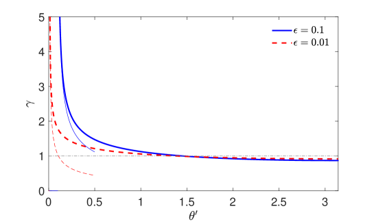
Figure 2: Coefficient of variation $\gamma=\sqrt{{\rm var}(\mathcal{T}^{\rm surf})}/\langle\mathcal{T}^{\rm surf}\rangle$ as function of $\theta^{\prime}$ for the FPT to the target of angular size $\varepsilon$ by surface diffusion, for two values of $\varepsilon$. Thick lines represent the exact result from equations (13) and (14), while the thin lines show the asymptotic relation (15).

2.4 Asymptotic behaviour of equation (10)

Before we turn to the discussion of the ADS it is instructive to discuss the asymptotic behaviour of its constituents: $\tilde{j}(p,\mathbf{s}|\mathbf{x})$ in equation (6) and $\tilde{H}^{\rm surf}(p;\theta^{\prime})$ in equation (10). We will show that both exhibit some non-trivial and universal behaviour, which will permit us to reach several conclusive statements about the asymptotic behaviour of the full PDF $H^{\rm AD}(t;\mathbf{x})$.

We start with $\tilde{H}^{\rm surf}(p;\theta^{\prime})$ and consider first the limit $p\to\infty$, which corresponds to the short-$t$ tail of the associated PDF. In B we show that in this limit $\tilde{H}^{\rm surf}(p;\theta^{\prime})$ obeys

$$\tilde{H}^{\rm surf}(p;\theta^{\prime})\simeq\sqrt{\frac{\sin(\varepsilon)}{\sin(\theta^{\prime})}}\,e^{-R_{1}(\theta^{\prime}-\varepsilon)\sqrt{p/D_{s}}}\quad(p\to\infty)\,,$$ (17)

where the symbol $\simeq$ denotes that we consider the leading order of this limiting behaviour. Inverting the Laplace transform in the latter expression, we find that the short-$t$ asymptotic behaviour of the PDF $H^{\rm surf}(t;\theta^{\prime})$ follows

$$H^{\rm surf}(t;\theta^{\prime})\simeq\sqrt{\frac{\sin(\varepsilon)}{\sin(\theta^{\prime})}}\,\frac{(\theta^{\prime}-\varepsilon)R_{1}}{\sqrt{4\pi D_{s}t^{3}}}\,e^{-(\theta^{\prime}-\varepsilon)^{2}R_{1}^{2}/(4D_{s}t)}.$$ (18)

Remarkably, this result coincides (up to the factor $\sqrt{\sin(\varepsilon)/\sin(\theta^{\prime})}$) with the celebrated Lévy-Smirnov distribution [48, 49], defining the exact FPT PDF from a point $x_{0}=(\theta^{\prime}-\varepsilon)R_{1}>0$ to a perfect target located at the origin of a one-dimensional semi-infinite line. Noticing that $R_{1}(\theta^{\prime}-\varepsilon)$ is, in fact, the geodesic distance between the point $\mathbf{s}$ and the boundary of the target region, i.e., the shortest path along the surface of the inner sphere from the starting point $\mathbf{s}$ to the target, its physical significance becomes apparent: the short-$t$ tails of the PDF are dominated by such trajectories which move diffusively along the shortest distance to the target. We note that such a Lévy-Smirnov-like form, which is specific to one-dimensional situations, has been previously evidenced for rather different two- and three-dimensional geometrical settings (see, e.g., [64, 65, 66, 62, 63, 81]) and therefore seems to be quite generic. In particular, this result is analogous to the "geometry control" unveiled previously in the case of pure bulk diffusion in $\Omega$ [62, 64].

In turn, the leading long-$t$ behaviour of the PDF $H^{\rm surf}(t;\theta^{\prime})$ can be readily deduced from the series representation in equation (2.3). Recalling that the solutions $\nu_{n}$ form an increasing sequence, we realise that at long times the dominant contribution corresponds to the smallest root $\nu_{0}$ of equation (12) and, therefore, the long-$t$ behaviour reads

$$H^{\rm surf}(t;\theta^{\prime}) \simeq\frac{\sin^{2}(\varepsilon)D_{s}}{R_{1}^{2}}\left(\int^{1}_{-\cos(\varepsilon)}dx\left[P_{\nu_{0}}(x)\right]^{2}\right)^{-1/2}P_{\nu_{0}}(-\cos(\theta^{\prime}))P^{\prime}_{\nu_{0}}(-\cos(\varepsilon))$$

$$\quad\times e^{-\nu_{0}(\nu_{0}+1)D_{s}t/R^{2}_{1}}.$$ (19)

We note that $\nu_{0}$ depends on $\varepsilon$ but is independent of $\theta^{\prime}$; in particular when $\varepsilon$ is small, one has $\nu_{0}\approx 1/(2\ln(2/\varepsilon))$ [80]. As a consequence the longest relaxation time

$$\tau^{\rm surf}=\frac{R^{2}_{1}}{\nu_{0}(\nu_{0}+1)D_{s}}\approx\frac{2R_{1}^{2}\ln(2/\varepsilon)}{D_{s}}\quad(\varepsilon\ll 1)$$ (20)

is independent of the starting point, i.e., corresponds to such long times at which a particle arrives to the target region after extensive target-avoiding excursions and thus loses information about its initial location. The latter is kept only through the amplitude in equation (2.4).

2.5 Asymptotic behaviour of equation (6)

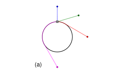
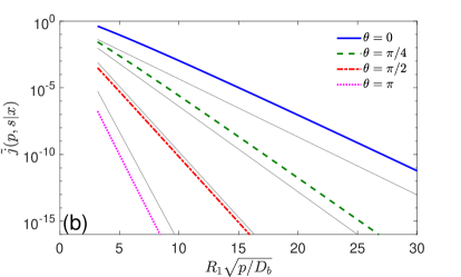
Figure 3: Large-$p$ asymptotic behaviour of $\tilde{j}(p,\mathbf{s}|\mathbf{x})$ in equation (6) for $\phi=\phi^{\prime}$. Panel (a): Shortest distances to the arrival point $\mathbf{s}$ located on the North pole (filled squares) from different starting points $\mathbf{x}$ (filled circles). Blue ($\theta=0$) and green ($\theta=\pi/4$) circles correspond to the case when $\mathbf{s}$ is directly visible from $\mathbf{x}$, such that the shortest distance ${\ell}_{\rm vis}$ (see the corresponding dotted lines) is given by the straight segment connecting the initial point and the arrival point $\mathbf{s}$. Red ($\theta=\pi/2$) and magenta ($\theta=\pi$) circles correspond to the situation in which the target appears on the "dark" side of the inner sphere with respect to the initial point. In this case the shortest distance ${\ell}_{\rm invis}$ consists of two parts: A straight segment of length $h=\sqrt{r^{2}-R_{1}^{2}}$ from the initial point to the point closest to the target on the horizon, and an arc from this point to the target. Panel (b): Numerical analysis of $\tilde{j}(p,\mathbf{s}|\mathbf{x})$ in equation (6) as function of $R_{1}\sqrt{p/D_{b}}$. Coloured thick curves present $\tilde{j}(p,\mathbf{s}|\mathbf{x})$ obtained by summing the series in equation (6) truncated at $n_{\rm max}=100$. As we are interested in the large-$p$ behaviour, we set $R_{2}=\infty$ here to ease the numerical computation of the radial functions $g_{n}^{(p)}(r)$. Thin grey lines show the asymptotic forms in equation (21) and (22) with the shortest distances calculated for the corresponding geometrical setup (note that the unknown functions $a(\theta,\theta^{\prime})$ and $b(\theta,\theta^{\prime})$, controlling a vertical offset of these lines, were set to $1$).

Let us now turn to the joint probability density $j(t,\mathbf{s}|\mathbf{x})$. A theoretical analysis of the large-$p$ asymptotic behaviour of expression (6) appears to be a difficult task; we realise that, in fact, in order to determine the corresponding asymptotic form one has to perform the sum in this equation exactly, which requires a cumbersome analysis. We thus resort instead to a numerical analysis of expression (6) aiming to verify the following conjecture: we assume that, in line with the "geometrical optics" arguments presented earlier in [82] (see section II) and similarly to the above considered case of a search process on the surface of a sphere, the short-$t$ tail of the associated PDF corresponds to the diffusive motion along the shortest path (with length ${\ell}$) from $\mathbf{x}=(r,\theta,\phi)$ to $\mathbf{s}=(R_{1},\theta^{\prime},\phi^{\prime})$. This path, however, has a different form depending on whether the point $\mathbf{s}$ is directly "visible" from $\mathbf{x}$, i.e., is located within a spherical cap region delimited by the horizon, or whether it is located outside of this area being situated on the "dark" side of the inner sphere and therefore invisible from $\mathbf{x}$. In case when $\mathbf{s}$ is visible from $\mathbf{x}$ we thus expect that

$$\tilde{j}(p,\mathbf{s}|\mathbf{x})\simeq a(\theta,\theta^{\prime})e^{-{\ell}_{\rm vis}\sqrt{p/D_{b}}}\quad(p\to\infty),$$ (21)

where $a(\theta,\theta^{\prime})$ is some unknown amplitude (recall that the result in equation (18) differs from the standard Lévy-Smirnov density by some function) and ${\ell}_{\rm vis}$ is the Euclidean distance from $\mathbf{x}$ to $\mathbf{s}$. In turn, for the case when $\mathbf{s}$ is located on the "dark" side, the shortest path ${\ell}_{\rm invis}$ consists of two parts (see also [82]): the particle diffuses along a straight line of length $h=\sqrt{r^{2}-R_{1}^{2}}$ connecting $\mathbf{x}$ and the point on the horizon, which is closest to $\mathbf{s}$, and then travels diffusively in the immediate vicinity of the inner sphere along the arc connecting this point on the horizon and $\mathbf{s}$. Consequently, in this case we expect that $\tilde{j}(p,\mathbf{s}|\mathbf{x})$ behaves in the limit $p\to\infty$ as

$$\tilde{j}(p,\mathbf{s}|\mathbf{x})\simeq b(\theta,\theta^{\prime})e^{-{\ell}_{\rm invis}\sqrt{p/D_{b}}}\quad(p\to\infty),$$ (22)

where $b(\theta,\theta^{\prime})$ is an unknown amplitude. Note that ${\ell}_{\rm vis}$ and ${\ell}_{\rm invis}$ can be simply expressed through the Cartesian coordinates of both points.

In figure 3 we compare our conjectured equations (21) and (22) (thin grey lines) and the exact expression (thick coloured curves) obtained from series truncation in equation (6) for two situations in which the target is visible from the starting point, and two situations in which it is located on the dark side. We observe that in all four cases the slopes of thin grey lines and of the thick coloured curves are almost identical—which thus confirms our conjecture of the large-$p$ behaviour of $\tilde{j}(p;\mathbf{s}|\mathbf{x})$. Inverting the expressions in equations (21) and (22), we thus find that the short-$t$ behaviour of the corresponding PDF $j(t;\mathbf{s}|\mathbf{x})$ has the Lévy-Smirnov form ${\ell}\exp(-{\ell}^{2}/(4D_{b}t))/\sqrt{4\pi D_{b}t^{3}}$, up to a yet unknown amplitude factor $a(\theta,\theta^{\prime})$ or $b(\theta,\theta^{\prime})$, respectively.

Lastly, we discuss the long-$t$ behaviour of the PDF $j(t,\mathbf{s}|\mathbf{x})$. As diffusion occurs in a bounded domain, $j(t,\mathbf{s}|\mathbf{x})$ clearly exhibits an exponential decay which is controlled by the pole $p_{0}^{\rm bulk}$ of $\tilde{j}(p,\mathbf{s}|\mathbf{x})$ with the smallest absolute value. This is actually the pole of the radial function $g_{0}^{(p)}(r)$, which can be written as

$$p_{0}^{\rm bulk}=-\frac{1}{\tau^{\rm bulk}}<0,\mbox{ with }\tau^{\rm bulk}=\frac{(R_{2}-R_{1})^{2}}{D_{b}\alpha_{0}^{2}},$$ (23)

where $\alpha_{0}$ is the smallest root of the transcendental equation (see, e.g., [64])

$$\frac{\tan(\alpha_{0})}{\alpha_{0}}=\frac{R_{2}}{R_{2}-R_{1}}.$$ (24)

When $R_{1}\ll R_{2}$, this solution behaves as $\alpha_{0}^{2}\approx R_{1}/(3(R_{2}-R_{1}))$ and thus

$$\tau^{\rm bulk}\approx\frac{R_{2}^{3}}{3D_{b}R_{1}}.$$ (25)

Therefore, in the long-$t$ limit the PDF $j(t,\mathbf{s}|\mathbf{x})$ decays as

$$j(t,\mathbf{s}|\mathbf{x})\propto e^{-t/\tau^{\rm bulk}},$$ (26)

where $\tau^{\rm bulk}$ is the longest time characterising the FPT PDF to the inner sphere conditioned by the constraint that this event took place at point $\mathbf{s}$. Note that $\tau^{\rm bulk}$ is independent of both the initial position $\mathbf{x}$ and the precise location of the arrival point $\mathbf{s}$. Some other properties of the probability flux density $j(t,\mathbf{s}|\mathbf{x})$ were discussed in a recent paper [83].

3 Probability density function of the first-passage times within the Adam-Delbrück scenario

In this section we focus on the statistics of the FPTs in the ADS. We start from our main relation (2.2), in which the integral over the first arrival point $\mathbf{s}$ on the inner sphere can be further simplified (see details in C) to get the exact and fully explicit solution in the Laplace domain

$$\tilde{H}^{\rm AD}(p;\mathbf{x}) =\sum\limits_{n=0}^{\infty}g_{n}^{(p)}(r)P_{n}(\cos\theta)\biggl{\{}\frac{P_{n-1}(\cos\varepsilon)-P_{n+1}(\cos\varepsilon)}{2}$$

$$-(1-\cos^{2}\varepsilon)\frac{n+1/2}{\frac{pR^{2}}{D_{s}}+n(n+1)}\,\biggl{(}P^{\prime}_{n}(\cos\varepsilon)+P_{n}(\cos\varepsilon)\frac{P^{\prime}_{\mu}(a)}{P_{\mu}(a)}\biggr{)}\biggr{\}}.$$ (27)

We first discuss the short-$t$ and long-$t$ asymptotic behaviour of the PDF $H^{\rm AD}(t;\mathbf{x})$. Next, numerically inverting the Laplace transform in equation (27) by help of the Talbot algorithm we discuss the behaviour of the PDF in the time domain for different values of the system parameters and compare it against the recently obtained PDF for the direct search scenario in precisely the same geometrical settings [50]. This will give us a general idea of the shapes of two PDFs. Moreover, we turn to the integrated characteristic—the survival probability

$$S^{\rm AD}(t;\mathbf{x})=\int\limits_{t}^{\infty}dt^{\prime}\,H^{\rm AD}(t^{\prime};\mathbf{x}),$$ (28)

i.e., the probability that the target is not found up to time $t$. The analysis of the survival probability for both search scenarios provides a full understanding of the actual efficiency of each scenario and, hence, gives an idea which scenario is more successful. In the Laplace domain, the survival probability in equation (28) reads $\tilde{S}^{\rm AD}(p;\mathbf{x})=(1-\tilde{H}^{\rm AD}(p;\mathbf{x}))/p$, allowing us to determine its asymptotic properties from those for the Laplace-transformed PDF. The analysis of the survival probability will permit us to make several conclusive statements. Lastly, we consider the particular, experimentally relevant case when the starting point is uniformly distributed on a spherical surface of radius $r$ such that $0<R_{1}\leq r\leq R_{2}$. Moreover, in C we present additional figures illustrating the behaviour of $H^{\rm AD}(t^{\prime};\mathbf{x})$ for several fixed starting points of the ligand.

3.1 Asymptotic behaviour

To access the short-$t$ behaviour of $H^{\rm AD}(t;\mathbf{x})$ we focus on expression (2.2) together with equations (17), (21), and (22). Combining these expressions, we get the Laplace-transformed PDF $\tilde{H}^{\rm AD}(p;\mathbf{x})$ in the limit $p\to\infty$ in the form

$$\tilde{H}^{\rm AD}(p;\mathbf{x}) \approx\sqrt{\sin(\varepsilon)}\int_{\partial\Omega_{\rm vis}}d\mathbf{s}\frac{a(\theta,\theta^{\prime})}{\sqrt{\sin(\theta^{\prime})}}\exp\left(-\left(\frac{{\ell}_{\rm vis}(r,\theta,\theta^{\prime})}{\sqrt{D_{b}}}+\frac{(\theta^{\prime}-\varepsilon)R_{1}}{\sqrt{D_{s}}}\right)\sqrt{p}\right)+$$

$$\sqrt{\sin(\varepsilon)}\int_{\partial\Omega_{\rm invis}}d\mathbf{s}\frac{b(\theta,\theta^{\prime})}{\sqrt{\sin(\theta^{\prime})}}\exp\left(-\left(\frac{{\ell}_{\rm invis}(r,\theta,\theta^{\prime})}{\sqrt{D_{b}}}+\frac{(\theta^{\prime}-\varepsilon)R_{1}}{\sqrt{D_{s}}}\right)\sqrt{p}\right),$$ (29)

where $\partial\Omega_{\rm vis}$ and $\partial\Omega_{\rm invis}$ denote the two parts of the inner sphere, those that are "visible" and "invisible" as seen from the starting point $\mathbf{x}$. In the limit $p\to\infty$ the integrands in equation (3.1) vanish exponentially fast with $p$. This signifies that the dominant contribution to the integrals comes from such values of the position $\mathbf{s}$ of the landing point onto the inner sphere for which the coefficients in front of $\sqrt{p}$ are minimal, i.e.,

$$\tilde{H}^{\rm AD}(p;\mathbf{x})\sim\exp\left(-\ell_{\rm min}\sqrt{p/D_{b}}\right),$$ (30)

where

$$\ell_{\rm min}=\min\limits_{\theta^{\prime}}\left\{\ell(r,\theta,\theta^{\prime})+R_{1}(\theta^{\prime}-\varepsilon)\sqrt{D_{b}/D_{s}}\right\},$$ (31)

where $\ell(r,\theta,\theta^{\prime})$ is either $\ell_{\rm vis}$ or $\ell_{\rm invis}$, depending on the mutual arrangement of $\mathbf{x}$ and $\mathbf{s}$. As a consequence, we expect that the short-$t$ tail of $H_{\rm AD}(t;\mathbf{x})$ has a universal Lévy-Smirnov form, yet with a position-specific prefactor.

As diffusion occurs in a bounded domain, the PDF $H^{\rm AD}(t;\mathbf{x})$ decays exponentially fast at long times, and the decay rate is determined by the pole $p_{0}<0$ of $\tilde{H}^{\rm AD}(p;\mathbf{x})$ with the smallest absolute value. Since $\tilde{H}^{\rm AD}(p;\mathbf{x})$ is obtained in equation (2.2) by integrating the product of $\tilde{j}(p,\mathbf{s}|\mathbf{x})$ and $\tilde{H}^{\rm surf}(p;\mathbf{s})$ over $\mathbf{s}$, $p_{0}$ is the pole of one of these two functions. Skipping technical details presented in C.2 we conclude that

$$H^{\rm AD}(t;\mathbf{x})\simeq C_{\varepsilon}(\mathbf{x})\exp\left(-\frac{t}{{\rm max}\left\{\tau^{\rm bulk},\tau^{\rm surf}\right\}}\right),$$ (32)

where the amplitude $C_{\varepsilon}(\mathbf{x})$ is explicitly computed in equations (100) and (104). Here ${\rm max}\left\{\tau^{\rm bulk},\tau^{\rm surf}\right\}$ signifies that the onset and the decay of the long-$t$ asymptotic form is entirely controlled by the longest of the two characteristic times $\tau^{\rm bulk}$ and $\tau^{\rm surf}$, but not by their sum, which, in contrast, is assumed in the conventional criterion of the applicability of the ADS. We finally note that the decay rate in equation (32) is independent of the starting point $\mathbf{x}$ for any relation between $\tau^{\rm bulk}$ and $\tau^{\rm surf}$.

3.2 Random starting point

In many situations of practical interest the launch of the ligand does not take place from a fixed prescribed position. Instead there are many points on the outer sphere from which the ligand can start its search for the target. In this regard it is instructive to consider the case when $\mathbf{x}$ can be any (uniformly-distributed) point on the spherical surface of radius $r$ (not necessarily the outer boundary, $r=R_{2}$). The behaviour of the FPT PDF corresponding to the case when the ligand starts from a prescribed position turns out to be quite similar, as discussed in C.4.

The Laplace-transformed PDF for a random starting point, which we denote as $\overline{\tilde{H}_{\rm AD}(p;r)}$, is obtained by integration of equation (27) over the angular coordinates of $\mathbf{x}$, yielding

$$\overline{\tilde{H}^{\rm AD}(p;r)} =\frac{1}{4\pi r^{2}}\int_{|\mathbf{x}|=r}d\mathbf{x}\,\tilde{H}^{\rm AD}(p;\mathbf{x})$$

$$=\frac{1-\cos(\varepsilon)}{2}g_{0}^{(p)}(r)\left(1-\frac{D_{s}(1+\cos(\varepsilon))}{pR_{1}^{2}}\frac{P^{\prime}_{\mu}(-\cos(\varepsilon))}{P_{\mu}(-\cos(\varepsilon))}\right),$$ (33)

where $g_{0}^{(p)}(r)$ and $\mu$ were defined in equations (7) and (10), respectively. We stress that this surface-averaged quantity differs from the volume average over a uniformly distributed starting point inside the confining domain $\Omega$.

The asymptotic behaviour of $\overline{\tilde{H}^{\rm AD}(p;r)}$ is derived in C and reads

$$\overline{H^{\rm AD}(t;r)} \simeq\frac{R_{1}}{r}\,\frac{(r-R_{1})}{\sqrt{4\pi D_{b}t^{3}}}\exp\left(-\frac{(r-R_{1})^{2}}{4D_{b}t}\right)$$

$$\times\biggl{(}\frac{1-\cos(\varepsilon)}{2}+\frac{\sin(\varepsilon)\sqrt{D_{s}D_{b}t^{2}}}{R_{1}(r-R_{1})}+\frac{\cos(\varepsilon)D_{b}D_{s}t^{2}}{R_{1}^{2}(r-R_{1})^{2}}\biggr{)}.$$ (34)

The prefactor in the first line is the PDF of the FPT to a perfectly reactive sphere of radius $R_{1}$ by bulk diffusion in a three-dimensional unbounded domain. At very short times, the first term is dominant, and one gets, up to a geometric prefactor $(1-\cos(\varepsilon))R_{1}/(2r)$, the Lévy-Smirnov function of $t$,

$$\overline{H^{\rm AD}(t;r)}\simeq\frac{(1-\cos(\varepsilon))R_{1}}{2r}\,\frac{(r-R_{1})}{\sqrt{4\pi D_{b}t^{3}}}\exp\left(-\frac{(r-R_{1})^{2}}{4D_{b}t}\right).$$ (35)

Interestingly, this short-$t$ tail of the PDF is independent of the surface diffusion coefficient $D_{s}$. Apparently, this is associated with the fact that when we average over the starting point, the major contribution to the PDF, which entirely defines its asymptotic behaviour, comes from those initial locations that are placed directly over the target site. The contributions from other starting points, for which the search process will include a tour of surface diffusion, is only sub-dominant in this limit. However, this leading-order contribution is attenuated by the prefactor $1-\cos(\varepsilon)\approx\varepsilon^{2}/2$, which can be very small for small targets. In turn, the second and third terms in equation (34), although being subleading in powers of time, are weighted by $\sin(\varepsilon)\approx\varepsilon$ and by $\cos(\varepsilon)\approx 1$, respectively. This means that when $\varepsilon$ is sufficiently small, there exists an intermediate range of times, for which the third term is actually the dominant one,

$$\overline{H^{\rm AD}(t;r)}\simeq\frac{D_{s}\sqrt{D_{b}t}}{\sqrt{4\pi}\,rR_{1}(r-R_{1})}\exp\left(-\frac{(r-R_{1})^{2}}{4D_{b}t}\right).$$ (36)

Curiously, this expression is independent of the target size (as soon as $\varepsilon$ is small). This is due to the fact that a decrease of $\varepsilon$ reduces the relative contribution of trajectories that arrive to the target directly from the bulk and thus avoid surface diffusion. Hence, for small $\varepsilon$ the search process will necessitate surface diffusion.

In the opposite long-time limit, there is no difference between the fixed and random starting point so that our former asymptotic relation (32) is valid for $\overline{H^{\rm AD}(t;r)}$.

Figure 4 illustrates the asymptotic behaviour of the surface-averaged PDF $\overline{H^{\rm AD}(t;r)}$ within the ADS. One sees that the asymptotic relation (34) accurately describes the short-time behaviour. As the target is rather small, the dominant contribution comes from the third term in equation (34); in particular, the three asymptotic curves only differ by the multiplicative factor $D_{s}$. We stress that the first term in equation (34) in this setting is totally irrelevant here (if one only kept the first term, the asymptotic curves would be below $10^{-6}$ and thus invisible in this figure; for this reason, they are not shown). In other words, the leading-order Lévy-Smirnov-type relation (35) fails, and one has to rely on our asymptotic relation (34), in which the third, sub-leading term is dominant. The long-time asymptotic relation (32) is also very accurate. Note that the amplitude $C_{\varepsilon}(r)$ is given by equation (104) for the curve with $D_{s}/D_{b}=1$, for which $\tau^{\rm bulk}>\tau^{\rm surf}$; in turn, it is given by equation (100) for the two other curves with $D_{s}/D_{b}=0.1$ and $D_{s}/D_{b}=0.01$. We conclude that both short- and long-time asymptotic relations are accurate.

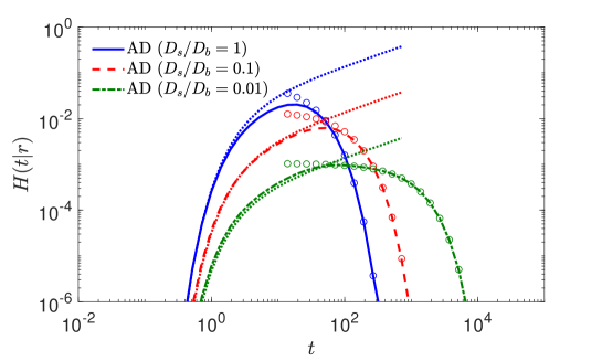
Figure 4: FPT PDF $\overline{H^{\rm AD}(t;r)}$ to a target of the small angular size $\varepsilon=0.01$ within the ADS, with $R_{2}/R_{1}=5$, for which the starting point is uniformly distributed over the outer sphere ($r/R_{1}=5$). The three thick coloured curves show the PDF obtained from the exact solution (33) via numerical inversion of the Laplace transform. Dotted lines represent the short-time asymptotic relation (34), whereas circles show the long-time asymptotic relation (32). The leading-order Lévy-Smirnov-type relation (35) is not shown because it lies below the bottom limit $10^{-6}$ of the plot; in fact, its maximal amplitude is $2.89\times 10^{-7}$, i.e., this approximation fails by 4 to 5 orders of magnitude. The length and time units are fixed by setting $R_{1}=1$ and $D_{b}=1$.

The derivative of $\overline{\tilde{H}^{\rm AD}(p;r)}$ in equation (33) with respect to $p$ determines the surface-averaged MFPT. Skipping the details of this computation (see C), the final result reads

$$\overline{T^{\rm AD}}=\frac{(r-R_{1})(2R_{2}^{3}-rR_{1}(r+R_{1}))}{6rR_{1}D_{b}}+\frac{R_{1}^{2}}{2D_{s}}\biggl{(}2\ln\biggl{(}\frac{2}{1-\cos\varepsilon}\biggr{)}-(1+\cos\varepsilon)\biggr{)}.$$ (37)

Here, the first term is the MFPT to the inner sphere, which is evidently independent of the target size. In turn, the second term is the contribution from the surface diffusion towards the target, averaged over the distribution of the first arrival point onto the surface (the so-called harmonic measure density). This contribution is independent of the radius $R_{2}$ of the outer sphere, as well as of the radial coordinate $r$ of the starting point. Expectedly, the second term vanishes as $\varepsilon\to\pi$ (the target covers the whole inner sphere) and diverges logarithmically as the target shrinks, $\varepsilon\to 0$. Note that if $r\gg R_{1}$, the diffusing ligand has sufficient time before hitting the inner sphere to loose the memory on its starting point, so that $T^{\rm AD}(\mathbf{x})\approx\overline{T^{\rm AD}}$. In other words, the explicit relation (37) can be used to estimate the MFPT from a fixed starting point $\mathbf{x}$ when it is located far from the inner sphere. Setting $r=R_{2}$, $R_{1}\ll R_{2}$ and $\varepsilon\ll 1$, one can easily check that $\overline{T^{\rm AD}}$ coincides, to the leading order, with $\tau_{\rm AD}$, which was discussed in section 1.

3.3 Comparison of the two search scenarios

We now compare the efficiency of the two search processes: ADS versus the direct search scenario. We focus on the case when the starting point is uniformly distributed over the outer sphere, for three reasons. (i) As discussed earlier, we keep in mind applications to microbiology, in which a particle enters the cytosol from the plasma membrane and searches for a nuclear pore; here, the spatial (angular) locations of the entrance channel and the nuclear pore are generally not known and can thus be modelled as random. (ii) When the inner sphere is small in comparison to the outer sphere (i.e, $R_{1}\ll R_{2}=r$), the particle has enough time to diffuse before hitting the inner sphere, and the information on the precise location of a fixed starting point is generally lost (except for very short trajectories determining the left, short-$t$ tail of the PDF)—in other words, in this setting, there is no notable difference between fixed and random starting points. (iii) The average over angular coordinates of the starting point eliminates all terms in the series representations (27) of the PDF, except for $n=0$, that facilitates its numerical computation and reduces eventual truncation errors (when an infinite series is replaced by a finite sum)—this is particularly relevant in case of a small target when one would have to keep a large number of terms to get accurate results, whereas the computation of the radial functions $g_{n}^{(p)}(r)$ may be problematic for large $n$. In C, we briefly discuss the case of a fixed starting point—which is conceptually important—and compare it to our main conclusions here for a random starting point.

The precise form of the Laplace transform $\overline{\tilde{H}^{\rm AD}(p;r)}$ is given in equation (33). While the exact solution $\overline{\tilde{H}^{\rm dir}(p;r)}$ for the direct search scenario was derived in [50], we use the approximate relations (113) and (115) for our discussion (see details in D). Note that the latter have a much simpler and explicit form, as compared to the exact solution (which requires a numerical inversion of matrices), and are remarkably accurate, as shown in [50]. In both cases the PDFs in the time domain are obtained via numerical inversion of the corresponding Laplace transforms using the Talbot algorithm. We set the angular size of the target equal to $\varepsilon=0.01$, which is approximately ten times bigger than the angular size of a typical nuclear pore. This choice of a larger value of $\varepsilon$ is due to some numerical limitations. In fact, going to very small values of $\varepsilon$ necessitates taking into account too many terms in equation (113) for the direct search, whose numerical accuracy cannot be properly controlled by our algorithm. Nevertheless, the considered value $\varepsilon=0.01$ allows us to illustrate the main features of the FPT PDF and compare the two search scenarios. We fix length and time units by setting $R_{1}=1$ and $D_{b}=1$ and investigate the effect of other parameters onto the PDFs and the survival probabilities.

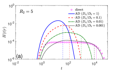
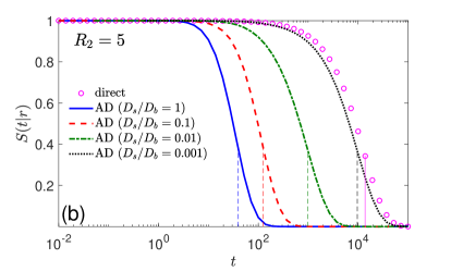
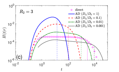
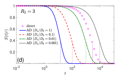
Figure 5: PDF (a,c) and associated survival probability (b,d) determining the FPT to a target of small angular size $\varepsilon=0.01$, with $R_{2}/R_{1}=5$ (a,b) (KR=0.008) or $R_{2}/R_{1}=3$ (c,d) (the KR= 0.037), and with a starting point uniformly distributed over the outer sphere ($r/R_{1}=5$). Comparison between the direct search (open circles, D) and the ADS (coloured curves corresponding to different values of the ratio $D_{s}/D_{b}$, see the legend). Vertical lines indicate the MFPTs given by equation (37) for the ADS and by equation (116) for the direct search. The numerical results for the direct search were obtained by using the approximate relation (131) with $n_{\rm inter}=50$ and $n_{\rm max}=250$ and by truncating the series (117) at $n_{\rm max}=2000$. Note that $\tau^{\rm surf}\approx 5.2/D_{s}$, whereas $\tau^{\rm bulk}\approx 29.3$ for $R_{2}/R_{1}=5$ and $\tau^{\rm bulk}\approx 4.7$ for $R_{2}/R_{1}=3$, i.e., $\tau_{\rm surf}$ is dominant for all cases except for $D_{s}/D_{b}=1$. Note that length and time units are fixed by setting $R_{1}=1$ and $D_{b}=1$.

Figure 5 illustrates our main results. Panels (a,b) correspond to the geometric setting with a small karyoplasmic ratio $\mathrm{KR}=0.008$ (with $R_{2}/R_{1}=5$), while panels (c,d) refer to the larger value $\mathrm{KR}=0.037$ (with $R_{2}/R_{1}=3$). Panels (a) and (c) present the FPT PDFs for both scenarios, with different values of the ratio $D_{s}/D_{b}$ (see the legends) and fixed angular size $\varepsilon=0.01$ of the target, offering insight into the functional form of the full PDFs, as well as of the locations of the most probable and mean FPTs (see the vertical dashed lines). For the ADS, the PDF is broadening with decreasing surface diffusion coefficient $D_{s}$. In fact, according to equation (35), the left short-time tail of the PDF is mainly controlled by bulk diffusion and thus does not change much with $D_{s}$. In turn, the right long-time tail is directly affected by $D_{s}$ via the time $\tau^{\rm surf}$ given by equation (20) which becomes dominant in equation (32) when $D_{s}$ is small enough. For instance, when $D_{s}/D_{b}=10^{-3}$ (which is appropriate for diffusion on hard solid surfaces), the PDF shown in panel (a) spans over five orders of magnitude in time. In turn, for larger $D_{s}$, the PDF of the ADS is more compact and attains substantially larger values in the vicinity of the most probable FPT than its counterpart for the direct search scenario. Decreasing $R_{2}/R_{1}$ from $5$ to $3$ (panels (c,d)) which results in the increase of the KR from $\mathrm{KR}\approx 0.008$ to $\mathrm{KR}\approx 0.037$, shifts the left tail of the PDF to the left (towards shorter times), because the target is now closer to the starting point. In turn, if $D_{s}$ is sufficiently small, the right tail of the distribution is still controlled by $\tau^{\rm surf}$, which is independent of $R_{2}$. As a consequence, the PDF is getting even broader.

While panels (a) and (c) present a basic conceptual understanding of the structure of the PDFs, panels (b) and (d) display the survival probability, which indeed proves to be a very robust measure of the relative efficiency of both search scenarios. We observe that for a small ratio $\mathrm{KR}=0.008$ and all considered values of $D_{s}/D_{b}$, the survival probabilities for the ADS, at any fixed $t$, are smaller than the survival probability of the target within the direct search scenario. In this situation, the ADS can be qualified as a more efficient search strategy as compared to the direct search. This conclusion also agrees with the fact that the MFPT for the direct search is longer than the MFPT within the ADS. Upon increase of KR (see the panel (d)), we notice that the ADS still outperforms the direct search scenario for $D_{s}/D_{b}\gtrsim 0.01$, and it becomes less efficient at $D_{s}/D_{b}=0.001$. Recall, however, that these curves are calculated for $\varepsilon=0.01$, which is somewhat higher than the typically encountered values of $\varepsilon$. On intuitive grounds, we may thus expect that for a smaller target with $\varepsilon=0.001$, as it is realised in the case of a nuclear pore, the ADS will perform better even in this case. Therefore, we demonstrate that the ADS can indeed be more efficient search scenario for quite reasonable values of the system parameters. We finally note that the survival probability at the MFPT appears to be quite universally equal to $0.35$, which signifies that two-thirds of searching trajectories find the target before this time, and only the remaining one-third arrive to the target location at longer times.

We finish this section by the analysis of the effect of the target size on the shapes of the PDFs and the survival probabilities. Figure 6 presents these functions in the same setting, except that now the target is tenfold larger, $\varepsilon=0.1$. As we already remarked, such a large value of $\varepsilon$ can be indicative of the behaviour in situations in which approximately $100$ nuclear pores are present on the surface of the nucleus. Remarkably, the PDFs within the ADS remain nearly the same as for a smaller target without any visible change, as compared to figure 5. At first thought, this is a counter-intuitive behaviour. However, we recall that the right tail of the PDF is mainly determined by $\tau^{\rm surf}$, which changes logarithmically slowly at small $\varepsilon$. In fact, as discussed in [80], $\nu_{0}\approx 1/(2\ln(2/\varepsilon))$ as $\varepsilon\to 0$ so that $\tau^{\rm surf}\approx 2R_{1}^{2}\ln(2/\varepsilon)/D_{s}$. Moreover, as we saw in section 3.2, the left tail of the distribution is also weakly dependent on the target size. For instance, the PDFs for even smaller target size $\varepsilon=0.001$, which is representative of the nuclear pore, are expected to be similar to those shown in figure 5. In contrast, the FPT PDF for the direct search scenario depends much more strongly on the target size. In fact, its right tail is characterised by the decay time, which is of the order of the MFPT and thus scales as $1/\varepsilon$. The amplitude of the left tail is also affected by $\varepsilon$. We thus observe that the efficiency of the ADS is weakly dependent on the target size and mainly controlled by two ratios $R_{1}/R_{2}$ and $D_{s}/D_{b}$. Overall, we conclude that in the case of larger targets the ADS outperforms the direct search scenario for $D_{s}/D_{b}\gtrsim 0.01$ (when $R_{2}/R_{1}=5$) and $D_{s}/D_{b}\gtrsim 0.1$ (when $R_{2}/R_{1}=3$), and is less efficient otherwise.

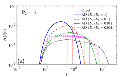
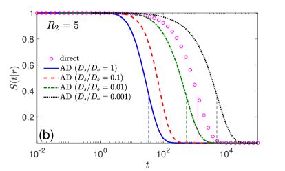
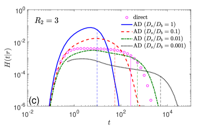
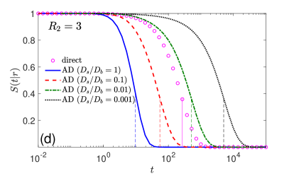
Figure 6: Same as in figure 5 but for a larger target with $\varepsilon=0.1$.

4 Amplified signals

We now extend our analysis to the important case of so-called "amplified" signals, when $N>1$ independently diffusing ligands search for a single target. We note that the ensuing speed-up of the search process has been intensively studied in rather diverse geometrical settings (different from our setting here) for the direct search scenario [84, 85, 86, 87, 88, 89, 90, 91, 92]. We start by introducing auxiliary notations and formulating some basic general results.

Let $\mathcal{T}_{i}$ (with $i=1,2,\ldots,N$) denote the time instant when the $i$th ligand arrives to the target for the first time. Consequently, the target is considered to be "found" when the fastest of the $N$ particles arrives to the target location, i.e., $\mathcal{T}=\min\{\mathcal{T}_{1},\mathcal{T}_{2},\ldots,\mathcal{T}_{N}\}$. Moreover, if all ligands start from the same fixed point $\mathbf{x}$, the survival probability that determines the probability law of the fastest FPT (fFPT) is given by

$$S^{\rm AD}_{N}(t;\mathbf{x})=\mathbb{P}\{\mathcal{T}>t\}=\mathbb{P}\{\mathcal{T}_{1}>t,\mathcal{T}_{2}>t,\ldots,\mathcal{T}_{N}>t\}=[S^{\rm AD}(t;\mathbf{x})]^{N},$$ (38)

where we took advantage of a physically plausible assumption that all ligands move independently of each other. If, in contrast, each ligand starts from a random position, which is uniformly distributed on a sphere of radius $r$, independently from the positions of the other ligands, then we have

$$\overline{S^{\rm AD}_{N}(t;r)}=\mathbb{P}\{\mathcal{T}>t\}=\mathbb{P}\{\mathcal{T}_{1}>t,\mathcal{T}_{2}>t,\ldots,\mathcal{T}_{N}>t\}=\left[\overline{S^{\rm AD}(t;r)}\right]^{N}.$$ (39)

In both cases, the associated PDFs are given by the time derivative

$$\begin{split}H^{\rm AD}_{N}(t;\mathbf{x})=N[S^{\rm AD}(t;\mathbf{x})]^{N-1}\,H^{\rm AD}(t;\mathbf{x}),\\ \overline{H^{\rm AD}_{N}(t;r)}=N\left[\overline{S^{\rm AD}(t;r)}\right]^{N-1}\,\overline{H^{\rm AD}(t;r)}.\end{split}$$ (40)

These two expressions allow for a detailed comparison of both scenarios in the amplified signal case, as presented in figure 7. Expressions (40) signify that, once the survival probability for a single ligand is found in the time domain—as evaluated in the previous sections—one has ready access to the statistics of the fFPT $\mathcal{T}$. Note, however, that the large-$N$ asymptotic analysis of the moments of $\mathcal{T}$ is more cumbersome (see, e.g., [84, 89] in the direct search case).

Panels (a) and (c) of figure 7 depict the PDF $\overline{H^{\rm AD}_{N}(t;r)}$ for the case when the starting points of the ligands are uniformly distributed over the outer sphere. The geometric setting is the same as for figure 5 with $R_{2}/R_{1}=5$. We see that the qualitative comparison between the ADS and the direct search does not change much for $N=10$ and $N=100$; in particular, the PDF for the direct search is relatively close to that for the ADS with $D_{s}/D_{b}=10^{-3}$. As expected, all PDFs are narrowing with increasing $N$. This is expected from the asymptotic behaviour for a single ligand. In fact, the long-time relation (32) implies that

$$\overline{H^{\rm AD}_{N}(t;r)}\simeq N[C_{\varepsilon}(r)]^{N}\exp\bigl{(}-Nt/\max\{\tau^{\rm bulk},\tau^{\rm surf}\}\bigr{)}\qquad(t\to\infty),$$ (41)

i.e., the decay time is decreased by the factor $N$, and thus the right tail is shifted towards the left (to shorter times). In contrast, as the survival probability $\overline{S^{\rm AD}_{N}(t;r)}$ is close to unity at short times, the left tail is just multiplied by $N$ and does not shift, i.e.,

$$\overline{H^{\rm AD}_{N}(t;r)}\simeq N\,\overline{H^{\rm AD}(t;r)}\qquad(t\to 0).$$ (42)

This relation is valid for moderate values of $N$. In turn, when $N$ is very large, we expect the emergence of an intermediate range of times for which the factor $\left[\overline{S^{\rm AD}(t;r)}\right]^{N-1}$ cannot be replaced by unity and starts to affect the distribution of the fFPT.

In panels (b) and (d) we depict the corresponding survival probabilities. We observe that they exhibit essentially the same behaviour as those in the case $N=1$, except for the fact that an abrupt decay to zero starts at progressively earlier times. We also infer from figure 7 that, maybe somewhat counter-intuitively, the relative efficiency of both search scenarios is the same as in the case of a single particle. Thus, the ADS appears to be more efficient for all considered values of $D_{s}/D_{b}$. We recall, however, that the relative efficiency also depends on the ratio $R_{2}/R_{1}$, see section 3.3. Similar conclusions hold for $N$ particles started from a fixed point located far from the target (not shown).

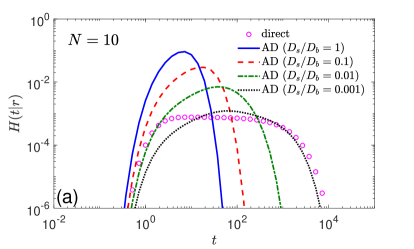
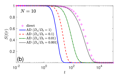
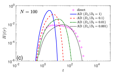
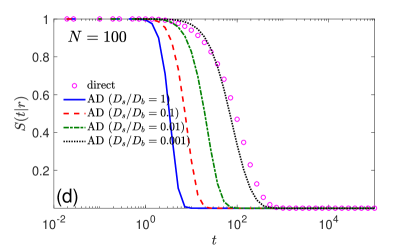
Figure 7: PDF (a,c) and associated survival probability (b,d) determining the fastest FPT to a target of small angular size $\varepsilon=0.01$, with $N=10$ (a,b) and $N=100$ (c,d) particles, $R_{2}/R_{1}=5$ (KR=0.008), and starting positions independently and uniformly distributed over the outer sphere ($r/R_{1}=5$). Comparison between the direct search (open circles, D) and the ADS (coloured curves corresponding to different values of the ratio $D_{s}/D_{b}$, see the legend). The numerical results for the direct search were obtained by using the approximate relation (131) with $n_{\rm inter}=50$ and $n_{\rm max}=250$.

5 Conclusions

For the simple geometrical setting of two nested, concentric and impenetrable spheres with an immobile target site being placed at the North pole of the inner sphere, we presented a detailed comparison of two search scenarios: (i) the direct search mode, when the particle needs to locate the target solely by bulk diffusion in the volume between the concentric spheres, with the surface of the inner sphere being perfectly reflecting, except for the target (see [50] for more details); and (ii) the Adam-Delbrück reduction-of-dimensionality scenario [1], for which the particle first attaches non-specifically to the reactive surface of the inner sphere and locates the target by diffusive search on the 2D surface. For both scenarios we calculate the FPT PDF for the searching ligand, that is initially released from a fixed point, or from a random position on the surface of the outer sphere. We also considered the case of "amplified" signals, when initially $N$ ligands are launched from the same fixed or random positions, and the search is completed when the fastest out of $N$ particles arrives to the target. Such settings indeed correspond to various situations and problems encountered in cellular biology, biophysics, and biochemistry. In particular, they appear as a crucial intermediate step in many signal transduction pathways in cellular environments.

To show that the reduction-of-dimensionality scenario may be beneficial in certain situations, Adam and Delbrück originally presented a comparison of the efficiency of both direct and ADS diffusive searches for a single ligand, judging solely from the mean times of diffusion towards the target site. In the present work confronting both scenarios, we went beyond the analysis of the MFPT—which by now is known to be non-representative in even simple geometries and sometimes even plainly misleading—and therefore focused our analysis on the PDF of the random individual FPTs from a fixed or a random starting position to the target. We compared the behaviour of the full FPT PDF as well as of their integrated characteristic, the survival probability, which appeared to be a robust measure of the actual efficiency of both search scenarios. In fact, if

$$S_{1}(t)\leq S_{2}(t)\qquad\forall\leavevmode\nobreak\ t\geq 0$$ (43)

for all times, the first search process (described by $S_{1}(t)$) is more efficient than the second one. As the MFPT is the integral of the survival probability, this inequality implies the conventional efficiency criterion,

$$T_{1}\leq T_{2},$$ (44)

in terms of the MFPTs $T_{1}$ and $T_{2}$ of two search processes. In this situation, both criteria are equivalent. However, the opposite claim is not true, namely, (44) does not imply (43). For instance, one may have $S_{1}(t)\leq S_{2}(t)$ at short times and $S_{1}(t)\geq S_{2}(t)$ at long times, even though $T_{1}=T_{2}$. In other words, one search process can be more efficient at short times and less efficient at long times. We conclude that the comparison of survival probabilities provides a more systematic and comprehensive insight into the search efficiency. On this basis, we specified realistic physical conditions in which the reduction-of-dimensionality scenario outperforms the direct search for both cases when a single ligand is present and when the signal is amplified.

Our analysis can be generalised in several directions. First, we considered exclusively the case of standard Brownian motion. In reality, both diffusion in the bulk and the surface diffusion may be (transiently) anomalous. These anomalous features can be incorporated in a standard way, e.g., via a subordination technique. Second, we supposed that the spherical-shell domain is a homogeneous liquid-filled region and does not contain any obstacles or "crowders". In turn, especially in cellular environments, this is not the case due to the presence of organelles, proteins and etc, which will certainly affect the dynamics [53]. Moreover, in some cases the cellular cytoplasm is actively moved by non-equilibrium action of molecular motors [93, 94, 95], thus changing the mixing dynamics inside the cell and creating dynamics heterogeneities [96, 97]. Consequently, these effects may alter the relative efficiency of both search scenarios in the realistic cellular setting. Third, both scenarios considered here pertain to two somewhat extreme situations: the particle is either perfectly reflected by the surface of the inner sphere or, in the ADS, non-specifically adsorbs to it upon first encounter. In reality, the situation can be more complex. As discussed recently in [70] within the context of a narrow-escape problem, there are distance-dependent potential interactions with the surface on which the target is located and the presence of such interactions modifies the search processes. As realised in [70], the most efficient interactions, i.e., resulting in the shortest FPT to the target, are neither too long-ranged not too short-ranged (as corresponds to the Adam-Delbrück picture) such that the optimal trajectories are intermittent—upon arrival to the inner sphere a ligand performs a finite surface diffusion tour and then desorbs to the bulk, arrives to the surface again, performing a new tour of surface diffusion, and so on, until the target is finally found. Even though such intermittent search strategies have been studied in the past (see, e.g., [32, 33, 34, 35, 36, 37, 38] and references therein), former works were almost exclusively focused on the mean FPT and the search optimality was qualified by its minimisation. In our future work, we will explore these possible generalisations of our present analysis.

Appendix A Moments of the conditioned first-passage time

The Laplace transform of the joint probability density $j(t,\mathbf{s}|\mathbf{x})$ in (6) determines all positive integer moments of the FPT $\mathcal{T}_{\mathbf{s}}$ to the inner sphere, conditioned by the arrival point $\mathbf{s}$,

$$\langle\mathcal{T}_{\mathbf{s}}^{k}\rangle=\int\limits_{0}^{\infty}dt\,t^{k}\,j(t,\mathbf{s}|\mathbf{x})=(-1)^{k}\lim\limits_{p\to 0}\frac{\partial^{k}}{\partial p^{k}}\tilde{j}(p,\mathbf{s}|\mathbf{x}).$$ (45)

One sees that it is sufficient to compute the Taylor expansion in powers of $p$ of the radial functions $g_{n}^{(p)}$ from (7). For instance, the first moment is given by

$$\langle\mathcal{T}_{\mathbf{s}}\rangle=-\frac{1}{4\pi R_{1}^{2}}\sum\limits_{n=0}^{\infty}(2n+1)P_{n}\left(\frac{(\mathbf{s}\cdot\mathbf{x})}{|\mathbf{s}|\,|\mathbf{x}|}\right)\lim\limits_{p\to 0}\frac{\partial g_{n}^{(p)}(r)}{\partial p}.$$ (46)

A lengthy but straightforward computation produces

$$\lim\limits_{p\to 0}\frac{\partial g_{n}^{(p)}(r)}{\partial p}=\frac{R_{2}^{2}}{4D_{b}}\,\frac{(n+1)(r/R_{2})^{n}+n(r/R_{2})^{-n-1}}{(n+1)(R_{1}/R_{2})^{n}+n(R_{1}/R_{2})^{-n-1}}\biggl{\{}\frac{1}{(n+1)(r/R_{2})^{n}+n(r/R_{2})^{-n-1}}$$

$$\times\biggl{[}\frac{n+1}{n+3/2}(r/R_{2})^{n+2}-\frac{n-1}{n-1/2}(r/R_{2})^{n}+\frac{n+2}{n+3/2}(r/R_{2})^{-n-1}-\frac{n}{n-1/2}(r/R_{2})^{-n+1}\biggr{]}$$

$$-\frac{1}{(n+1)(R_{1}/R_{2})^{n}+n(R_{1}/R_{2})^{-n-1}}\biggl{[}\frac{n+1}{n+3/2}(R_{1}/R_{2})^{n+2}$$

$$-\frac{n-1}{n-1/2}(R_{1}/R_{2})^{n}+\frac{n+2}{n+3/2}(R_{1}/R_{2})^{-n-1}-\frac{n}{n-1/2}(R_{1}/R_{2})^{-n+1}\biggr{]}\biggr{\}}.$$ (47)

The average of (46) over $\mathbf{s}$ results in the well-known expression for the MFPT to the inner sphere,

$$\int\limits_{{\partial\Omega}}d\mathbf{s}\,\langle\mathcal{T}_{\mathbf{s}}\rangle=-\lim\limits_{p\to 0}\frac{\partial g_{0}^{(p)}(r)}{\partial p}=\frac{(r-R_{1})(2R_{2}^{3}-rR_{1}(R_{1}+r))}{6D_{b}rR_{1}}.$$ (48)

Similarly, if the starting point $\mathbf{x}$ is uniformly distributed on a sphere of radius $r$, the integral over the angular coordinates in (46) cancels all terms with $n>0$, yielding

$$\frac{1}{4\pi r^{2}}\int\limits_{|\mathbf{x}|=r}d\mathbf{x}\,\langle\mathcal{T}_{\mathbf{s}}\rangle =-\frac{1}{4\pi R_{1}^{2}}\lim\limits_{p\to 0}\frac{\partial g_{0}^{(p)}(r)}{\partial p}$$

$$=\frac{1}{4\pi R_{1}^{2}}\,\frac{(r-R_{1})(2R_{2}^{3}-rR_{1}(R_{1}+r))}{6D_{b}rR_{1}},$$ (49)

which does not depend on the arrival point $\mathbf{s}$.

Note that when the starting point is located on the outer sphere, $r=R_{2}$, the first term in (47) is cancelled, and one gets the simpler expression

$$\lim\limits_{p\to 0}\frac{\partial g_{n}(R_{2})}{\partial p}=-\frac{R_{2}^{2}}{4D_{b}}\,\frac{(2n+1)(R_{1}/R_{2})^{n+1}}{\bigl{[}n+(n+1)(R_{1}/R_{2})^{2n+1}\bigr{]}^{2}}$$

$$\times\biggl{[}\frac{n+2}{n+3/2}-\frac{n}{n-1/2}(R_{1}/R_{2})^{2}-\frac{n-1}{n-1/2}(R_{1}/R_{2})^{2n+1}+\frac{n+1}{n+3/2}(R_{1}/R_{2})^{2n+3}\biggr{]}.$$

Appendix B Surface diffusion on the sphere

The problem of surface diffusion on a sphere has been intensively studied in the past (see [77, 78, 79, 80] and references therein). In particular, the exact solution for the concentration profile in the presence of a perfect target was given in [77, 78], whereas its extension to a partially reactive target with reversible binding was provided in [80]. Here we extend the derivation from [80] to get two equivalent representations of the FPT PDF for diffusion on the sphere.

Following [80], we consider diffusion on a sphere of radius $R$ (which is set to $R_{1}$ in the main text) towards a circular target of angular size $\varepsilon$ located on the South pole. This location is specific to this Appendix and differs from our consideration of the target on the North pole throughout the remaining text. This choice is taken for the fact that the solution will be given in terms of Legendre functions $P_{\nu}(x)$ with non-integer index $\nu$, which are regular at $x=1$ (the North pole) and singular at $x=-1$ (the South pole). As a consequence, it is natural to locate the target on the South pole to eliminate such singularities. Alternatively, one could search for the solution in terms of $P_{\nu}(1-x)$, which is equivalent to exchanging the North and South poles (i.e., by replacing the angle $\theta$ by $\pi-\theta$). Either way, once the derivation is completed, we will use such a swap to reformulate the final results for the target located on the North pole, to be consistent with the remainder of the paper.

We search for the Laplace-transformed survival probability $\tilde{S}^{\rm surf}(p;\mathbf{s})$ satisfying the boundary value problem

$$(p-D_{s}\Delta_{\mathbf{s}})\tilde{S}^{\rm surf}(p;\mathbf{s}) =1\quad(\theta>\pi-\varepsilon),$$ (50)

$$D_{s}\partial_{n}\tilde{S}^{\rm surf}(p;\mathbf{s})+\kappa_{s}\tilde{S}^{\rm surf}(p;\mathbf{s}) =0\quad(\theta=\pi-\varepsilon),$$ (51)

where $\mathbf{s}=(\theta,\phi)$ is a point on the sphere, $\pi-\varepsilon$ is the angular coordinate of the target region (here, it is a circle around the South pole), $\partial_{n}$ is the normal derivative oriented towards the South pole, $\Delta_{\mathbf{s}}$ is the Laplace-Beltrami operator, and $\kappa_{s}$ is the reactivity of the target. Even though the main text deals with a perfect target ($\kappa_{s}=\infty$), we here consider the more general case of a partially reactive target with a finite reactivity $\kappa_{s}$, from which the perfect target limit will follow. The axial symmetry of the problem implies that the survival probability depends only on the angle $\theta$ so that $\Delta_{\mathbf{s}}=\tfrac{1}{R^{2}}\mathcal{L}$, where

$$\mathcal{L}=\partial_{x}(1-x^{2})\partial_{x}\quad\mbox{ with }x=\cos\theta.$$ (52)

In the following, we will therefore write functions in terms of $x$, e.g., $\tilde{S}^{\rm surf}(p;x)$.

B.1 Two representations for the Green’s function

We start by considering the Green’s function for diffusion on the sphere, satisfying

$$(s-\mathcal{L})\tilde{G}(x,y|s)=\delta(x-y),\quad\bigl{(}\partial_{x}\tilde{G}(x,y|s)\bigr{)}|_{x=a}=\frac{qR}{\sqrt{1-a^{2}}}\tilde{G}(a,y|s),$$ (53)

where $s=pR^{2}/D_{s}$, $q=\kappa_{s}/D_{s}$, and $a=\cos(\pi-\varepsilon)=-\cos(\varepsilon)$ is the location of the target. The second relation is the Robin boundary condition on the partially reactive target. While $\tilde{G}(x,y|s)$ should be well known, we provide here the main steps of its derivation for the reader’s convenience.

On one hand, the Green’s function admits the spectral expansion over the Legendre functions $P_{\nu}(x)$ of the first kind which are the eigenfunctions of the operator $\mathcal{L}$, $\mathcal{L}P_{\nu}(x)=-\nu(\nu+1)P_{\nu}(x)$. One thus gets (see [80] for details)

$$\tilde{G}(x,y|s)=\sum\limits_{n=0}^{\infty}\frac{b_{n}^{2}\,P_{\nu_{n}}(x)\,P_{\nu_{n}}(y)}{s+\nu_{n}(\nu_{n}+1)}\quad(a\leq x\leq 1,a\leq y\leq 1),$$ (54)

where

$$b_{n}=\left(\int\limits_{a}^{1}dx\,[P_{\nu_{n}}(x)]^{2}\right)^{-1/2}$$ (55)

are the normalisation constants, and $\nu_{n}$ are the solutions of the equation

$$P^{\prime}_{\nu}(a)=\frac{qR}{\sqrt{1-a^{2}}}\,P_{\nu}(a)$$ (56)

that ensures the Robin boundary condition, and $P^{\prime}_{\nu}(a)=\bigl{(}\tfrac{\partial P_{\nu}(x)}{\partial x}\bigr{)}_{|x=a}$. We emphasise that the index $\nu$ of the Legendre function $P_{\nu}(x)$ is the unknown to be determined here. In the case of a perfect target ($q=\infty$), this relation becomes

$$P_{\nu}(a)=0.$$ (57)

One can easily check that the spectral expansion in (54) is the solution of (53). Indeed, the application of the operator $(s-\mathcal{L})$ to $\tilde{G}(x,y|s)$ yields

$$\sum\nolimits_{n=0}^{\infty}b_{n}^{2}\,P_{\nu_{n}}(x)\,P_{\nu_{n}}(y)=\delta(x-y)$$ (58)

due to the completeness relation for the eigenfunctions $P_{\nu_{n}}(x)$.

On the other hand, the Green’s function can be found as a combination of two linearly independent solutions of the homogeneous equation $(s-\mathcal{L})u=0$ which are given as $P_{\mu}(x)$ and $Q_{\mu}(x)$, where $Q_{\nu}(x)$ is the Legendre function of the second kind, and

$$\mu=\frac{-1+\sqrt{1-4s}}{2}$$ (59)

is the solution of the equation $s=-\nu(\nu+1)$ which satisfies $\mu\simeq-s$ in the limit $s\to 0$. One searches a solution of the form

$$\tilde{G}(x,y|s)=\left\{\begin{array}[]{ll}AP_{\mu}(x)&(y<x<1),\\ B\bigl{(}\hat{Q}P_{\mu}(x)-\hat{P}Q_{\mu}(x)\bigr{)}&(a<x<y),\end{array}\right.$$ (60)

with the shortcut notations $\hat{P}=P_{\mu}(a)-hP^{\prime}_{\mu}(a)$ and $\hat{Q}=Q_{\mu}(a)-hQ^{\prime}_{\mu}(a)$, where $h=\sqrt{1-a^{2}}/(qR)$. The first relation ensures the regularity of the solution at $x=1$, while the second relation takes care of the boundary condition (56) at $x=a$. The coefficients $A$ and $B$ are determined by requiring the continuity of $\tilde{G}(x,y|s)$ at $x=y$ and the drop by $1/(1-y^{2})$ of its derivative at $x=y$. One then finds

$$A =-\frac{\hat{Q}P_{\mu}(y)-\hat{P}Q_{\mu}(y)}{\hat{P}},$$ (61)

$$B =-\frac{P_{\mu}(y)}{\hat{P}},$$ (62)

where the Wronskian

$$P_{\nu}(y)Q^{\prime}_{\nu}(y)-P^{\prime}_{\nu}(y)Q_{\nu}(y)=\frac{1}{1-y^{2}}$$ (63)

was used. One finally finds

$$\tilde{G}(x,y|s)=\left\{\begin{array}[]{ll}P_{\mu}(x)\bigl{(}Q_{\mu}(y)-\frac{\hat{Q}}{\hat{P}}P_{\mu}(y)\bigr{)}&(y<x<1),\\ P_{\mu}(y)\bigl{(}Q_{\mu}(x)-\frac{\hat{Q}}{\hat{P}}P_{\mu}(x)\bigr{)}&(a<x<y).\end{array}\right.$$ (64)

Equating the right-hand sides of equations (54) and (64), one gets an identity which allows one to evaluate various series involving the zeros $\nu_{n}$ (see the review [98] for other examples and applications).

B.2 FPT distribution

In order to get the Laplace-transformed survival probability, it is sufficient to integrate the Green’s function $\tilde{G}(x,y|s)$ over $y$ from $a$ to $1$. For instance, the integral of (54) yields

$$\tilde{S}^{\rm surf}(p;x)=\frac{R^{2}}{D_{s}}\int\limits_{a}^{1}dy\,\tilde{G}(x,y|s)=\frac{R^{2}}{D_{s}}\sum\limits_{n=0}^{\infty}\frac{b_{n}^{2}\,P_{\nu_{n}}(x)(1-a^{2})P^{\prime}_{\nu_{n}}(a)}{\nu_{n}(\nu_{n}+1)(\frac{pR^{2}}{D_{s}}+\nu_{n}(\nu_{n}+1))},$$ (65)

where we used the identity

$$\int\limits_{a}^{b}dx\,P_{\nu}(x) =\frac{P_{\nu-1}(a)-P_{\nu+1}(a)-P_{\nu-1}(b)+P_{\nu+1}(b)}{2\nu+1}$$

$$=\frac{1-a^{2}}{\nu(\nu+1)}P^{\prime}_{\nu}(a)-\frac{1-b^{2}}{\nu(\nu+1)}P^{\prime}_{\nu}(b),$$ (66)

and a similar relation holds for $Q_{\nu}(x)$. Expression (65) was considered, e.g., in [80]. It can also be written as

$$\tilde{S}^{\rm surf}(p;x) =\frac{1}{p}\sum\limits_{n=0}^{\infty}b_{n}^{2}\,P_{\nu_{n}}(x)(1-a^{2})P^{\prime}_{\nu_{n}}(a)\biggl{(}\frac{1}{\nu_{n}(\nu_{n}+1)}-\frac{1}{\frac{pR^{2}}{D}+\nu_{n}(\nu_{n}+1)}\biggr{)}$$

$$=\frac{1}{p}\biggl{(}1-(1-a^{2})\sum\limits_{n=0}^{\infty}\frac{b_{n}^{2}\,P_{\nu_{n}}(x)\,P^{\prime}_{\nu_{n}}(a)}{\frac{pR^{2}}{D}+\nu_{n}(\nu_{n}+1)}\biggr{)},$$ (67)

where we evaluated explicitly the first sum by integrating (58) and using again (66). As a consequence, the Laplace-transformed PDF then becomes

$$\tilde{H}^{\rm surf}(p;x)=1-p\tilde{S}^{\rm surf}(p;x)=(1-a^{2})\sum\limits_{n=0}^{\infty}\frac{b_{n}^{2}P_{\nu_{n}}(x)P^{\prime}_{\nu_{n}}(a)}{\frac{R^{2}p}{D_{s}}+\nu_{n}(\nu_{n}+1)}.$$ (68)

The inverse Laplace transform can be easily found to be

$$H^{\rm surf}(t;x)=\frac{(1-a^{2})D_{s}}{R^{2}}\sum\limits_{n=0}^{\infty}b_{n}^{2}P_{\nu_{n}}(x)P^{\prime}_{\nu_{n}}(a)\,e^{-\nu_{n}(\nu_{n}+1)D_{s}t/R^{2}}.$$ (69)

This is a rare example of an exact explicit representation of the FPT PDF, except for a numerical step required to find the roots $\nu_{n}$. The MFPT can be formally deduced from the above equations, but it admits the simple closed-formed expression [78]

$$T^{\rm surf}(x)=\frac{R^{2}}{D}\ln\left(\frac{1+x}{1+a}\right)+\frac{R}{\kappa_{s}}\sqrt{\frac{1-a}{1+a}}.$$ (70)

While the series representation (68) of $\tilde{H}^{\rm surf}(p;x)$ was convenient for getting $H^{\rm surf}(t;x)$, another representation is needed for the analysis of the asymptotic behaviour. For this purpose, one can calculate $\tilde{S}^{\rm surf}(p;x)$ by integrating $\tilde{G}(x,y|s)$ from (64). After simplifications, we get

$$\tilde{S}^{\rm surf}(p;x)=\frac{1}{p}\biggl{(}1-\frac{P_{\mu}(x)}{P_{\mu}(a)-\frac{\sqrt{1-a^{2}}}{qR}P^{\prime}_{\mu}(a)}\biggr{)}$$ (71)

and thus

$$\tilde{H}^{\rm surf}(p;x)=\frac{P_{\mu}(x)}{P_{\mu}(a)-\frac{\sqrt{1-a^{2}}}{qR}P^{\prime}_{\mu}(a)}.$$ (72)

For a perfect target ($q=\infty$), one simply gets

$$\tilde{H}^{\rm surf}(p;x)=\frac{P_{\mu}(x)}{P_{\mu}(a)}.$$ (73)

Note that these solutions could be obtained directly by solving the related boundary value problems with the operator $\mathcal{L}$.

B.3 Short-time asymptotic behaviour

The above representation for $\tilde{H}^{\rm surf}(p;x)$ is suitable for getting the short-time asymptotic behaviour of the PDF. This corresponds to the large-$p$ limit, for which one can apply the asymptotic behaviour of the Legendre functions. Indeed, as $p\to\infty$, $\mu\simeq-\tfrac{1}{2}+i\sqrt{s}$ and we use

$$P_{\mu}(\cos\theta)\simeq\sqrt{\frac{\theta}{\sin\theta}}J_{0}((\,u+1/2)\theta)\approx\sqrt{\frac{\theta}{\sin\theta}}J_{0}(i\sqrt{s}\theta)=\sqrt{\frac{\theta}{\sin\theta}}I_{0}(\sqrt{s}\theta)\simeq\frac{e^{\sqrt{s}\,\theta}\,s^{-1/4}}{\sqrt{2\pi\sin\theta}},$$

from which equation (73) yields for a perfect target,

$$\tilde{H}^{\rm surf}(p;\theta)\simeq\sqrt{\frac{\sin\varepsilon}{\sin\theta}}\,e^{-(\theta-\varepsilon)R\sqrt{p/D_{s}}}\quad(p\to\infty).$$ (74)

The leading exponential term here is expected, given that $(\theta-\varepsilon)R$ is the geodesic distance between the starting point and the target. As a consequence, we get

$$H^{\rm surf}(t;\theta)\simeq\sqrt{\frac{\sin\varepsilon}{\sin\theta}}\,\frac{R(\theta-\varepsilon)e^{-R^{2}(\theta-\varepsilon)^{2}/(4D_{s}t)}}{\sqrt{4D_{s}t^{3}}}\quad(t\to 0).$$ (75)

B.4 Green’s function in absence of the target

As mentioned in the main text, the self-consistent approximation (121) can also be expressed in terms of Legendre functions. For this purpose, we need some identities that can be derived from the Green’s function without the target. In the limit $\varepsilon\to 0$ (or $a\to-1$), the Green’s function approaches

$$\tilde{G}(x,y|s)=\left\{\begin{array}[]{ll}P_{\mu}(x)\bigl{(}Q_{\mu}(y)-P_{\mu}(y)C_{\mu}\bigr{)}&(y<x<1),\\ P_{\mu}(y)\bigl{(}Q_{\mu}(x)-P_{\mu}(x)C_{\mu}\bigr{)}&(-1<x<y),\end{array}\right.$$ (76)

with

$$C_{\mu}=\lim\limits_{a\to-1}\frac{Q_{\mu}(a)}{P_{\mu}(a)}=\frac{\pi}{2\,\tan(\pi\mu)},$$ (77)

where we used the asymptotic behaviour of Legendre functions (see [99], p. 164). At the same time, this Green’s function admits the spectral expansion over Legendre polynomials $P_{n}(x)$,

$$\tilde{G}(x,y|s)=\sum\limits_{n=0}^{\infty}\frac{(n+1/2)\,P_{n}(x)\,P_{n}(y)}{s+n(n+1)}.$$ (78)

The integral of $\tilde{G}(x,y|s)$ over $y$ from $a$ to $1$, for $a<x<1$ yields the identity

$$\frac{1}{2}\sum\limits_{n=0}^{\infty}\frac{P_{n}(x)\,(P_{n-1}(a)-P_{n+1}(a))}{s+n(n+1)}=\frac{1}{s}\biggl{(}1-(1-a^{2})P_{\mu}(x)\bigl{(}Q^{\prime}_{\mu}(a)-C_{\mu}P^{\prime}_{\mu}(a)\bigr{)}\biggr{)},$$ (79)

where we used the identity (66). We emphasise that the condition $a<x<1$ should be satisfied, otherwise the identity does not hold. In the opposite case, one needs to integrate $\tilde{G}(x,y|s)$ over $y$ from $-1$ to $a$, to get for $-1<x<a$ that

$$\frac{1}{2}\sum\limits_{n=0}^{\infty}\frac{P_{n}(x)\,(P_{n-1}(a)-P_{n+1}(a))}{s+n(n+1)}=-\frac{(1-a^{2})P^{\prime}_{\mu}(a)\bigl{(}Q_{\mu}(x)-C_{\mu}P_{\mu}(x)\bigr{)}}{s}.$$ (80)

The integral of (79) over $x$ from $a$ to $1$ yields another identity,

$$\frac{1}{2}\sum\limits_{n=0}^{\infty}\frac{(P_{n-1}(a)-P_{n+1}(a))^{2}}{(2n+1)(s+n(n+1))}=\frac{(1-a^{2})^{2}P^{\prime}_{\mu}(a)\bigl{(}Q^{\prime}_{\mu}(a)-C_{\mu}P^{\prime}_{\mu}(a)\bigr{)}}{s^{2}}+\frac{1-a}{s}.$$ (81)

Note that the derivatives $P^{\prime}_{\nu}(x)$ and $Q^{\prime}_{\nu}(x)$ can be rewritten using the recurrence relations,

$$(2\nu+1)(1-x^{2})P^{\prime}_{\nu}(x) =\nu(\nu+1)(P_{\nu-1}(x)-P_{\nu+1}(x)),$$ (82)

$$(2\nu+1)(1-x^{2})Q^{\prime}_{\nu}(x) =\nu(\nu+1)(Q_{\nu-1}(x)-Q_{\nu+1}(x)).$$ (83)

Finally, integrating the representation of the Dirac distribution,

$$\frac{1}{2}\sum\limits_{n=0}^{\infty}(2n+1)P_{n}(x)P_{n}(y)=\delta(x-y)$$ (84)

over $y$ from $a$ to $1$, yields

$$\frac{1}{2}\sum\limits_{n=0}^{\infty}P_{n}(x)(P_{n-1}(a)-P_{n+1}(a))=\Theta(x-a),$$ (85)

where $\Theta(x-a)$ is the Heaviside step function.

Appendix C Solution for the Adam-Delbrück’s scenario

We here start from the convolution-like relation (2.2) and show how the integral over the arrival point on the inner sphere can be evaluated. We recall that the Laplace transforms $\tilde{j}(p,\mathbf{s}|\mathbf{x})$ and $\tilde{H}^{\rm surf}(p;\mathbf{s})$ were given by the explicit relations (6) and (10). To proceed, we use the addition theorem for (normalised) spherical harmonics $Y_{mn}(\theta,\phi)$,

$$\frac{2n+1}{4\pi}P_{n}\left(\frac{(\mathbf{s}\cdot\mathbf{x})}{|\mathbf{s}|\,|\mathbf{x}|}\right)=\sum\limits_{m=-n}^{n}Y_{mn}^{*}(\theta,\phi)Y_{mn}(\theta^{\prime},\phi^{\prime}),$$ (86)

where $\mathbf{x}=(r,\theta,\phi)$ and $\mathbf{s}=(R_{1},\theta^{\prime},\phi^{\prime})$. We substitute this expression into equation (6) and then into equation (2.2). As $\tilde{H}^{\rm surf}(p;\theta^{\prime})$ does not depend on $\phi^{\prime}$ due to the axial symmetry, the integral over $\phi^{\prime}$ cancels all contributions in the sum over $m$, except for $m=0$:

$$\tilde{H}^{\rm AD}(p;\mathbf{x}) =\int\limits_{0}^{\pi}d\theta^{\prime}\,\sin\theta^{\prime}\int\limits_{0}^{2\pi}d\phi^{\prime}\,\sum\limits_{n=0}^{\infty}g_{n}^{(p)}(r)\sum\limits_{m=-n}^{n}Y_{mn}^{*}(\theta,\phi)Y_{mn}(\theta^{\prime},\phi^{\prime})\,\tilde{H}^{\rm surf}(p;\theta^{\prime})$$

$$=\sum\limits_{n=0}^{\infty}g_{n}^{(p)}(r)(n+1/2)P_{n}(\cos\theta)\,c_{n}^{(p)}(\varepsilon),$$

where

$$c_{n}^{(p)}(\varepsilon) =\int\limits_{0}^{\pi}d\theta^{\prime}\,\sin\theta^{\prime}\,P_{n}(\cos\theta^{\prime})\,\tilde{H}^{\rm surf}(p;\theta^{\prime})$$

$$=\int\limits_{0}^{\varepsilon}d\theta^{\prime}\,\sin\theta^{\prime}P_{n}(\cos\theta^{\prime})+\frac{1}{P_{\mu}(a)}\int\limits_{\varepsilon}^{\pi}d\theta^{\prime}\,\sin\theta^{\prime}\,P_{n}(\cos\theta^{\prime})P_{\mu}(\cos(\pi-\theta^{\prime}))$$

$$=\frac{P_{n-1}(\cos\varepsilon)-P_{n+1}(\cos\varepsilon)}{2n+1}+\frac{(-1)^{n}}{P_{\mu}(a)}I_{n}^{(p)}(-\cos\varepsilon),$$

with

$$I_{n}^{(p)}(a)=\int\limits_{a}^{1}dx\,P_{n}(x)P_{\mu}(x),$$ (87)

where we used $P_{n}(-x)=(-1)^{n}P_{n}(x)$. Multiplying the Legendre equation for $P_{\mu}(x)$ by $P_{n}(x)$, subtracting its symmetrised version, and integrating over $x$ from $a$ to $1$, one immediately finds

$$I_{n}^{(p)}(a)=(1-a^{2})\frac{P^{\prime}_{n}(a)P_{\mu}(a)-P^{\prime}_{\mu}(a)P_{n}(a)}{n(n+1)-\mu(\mu+1)}.$$ (88)

Substituting this expression, we get

$$c_{n}^{(p)}(\varepsilon) =\frac{P_{n-1}(\cos\varepsilon)-P_{n+1}(\cos\varepsilon)}{2n+1}-\frac{1-\cos^{2}\varepsilon}{\frac{pR^{2}}{D_{s}}+n(n+1)}\,\frac{P^{\prime}_{n}(\cos\varepsilon)P_{\mu}(a)+P_{n}(\cos\varepsilon)P^{\prime}_{\mu}(a)}{P_{\mu}(a)},$$ (89)

where we used $P^{\prime}_{n}(-x)=(-1)^{n+1}P^{\prime}_{n}(x)$, and $-\mu(\mu+1)=pR^{2}/D_{s}$.

The additive structure of the coefficients $c_{n}^{(p)}(\varepsilon)$ suggests to represent $\tilde{H}^{\rm AD}(p;\mathbf{x})$ as a linear combination of the two contributions

$$\tilde{H}^{\rm AD}(p;\mathbf{x})=\tilde{H}_{1}(p;\mathbf{x})-\tilde{H}_{2}(p;\mathbf{x}),$$ (90)

where

$$\tilde{H}_{1}(p;\mathbf{x}) =\frac{1}{2}\sum\limits_{n=0}^{\infty}g_{n}^{(p)}(r)P_{n}(\cos\theta)\bigl{[}P_{n-1}(\cos\varepsilon)-P_{n+1}(\cos\varepsilon)\bigr{]},$$

$$\tilde{H}_{2}(p;\mathbf{x}) =(1-\cos^{2}\varepsilon)\sum\limits_{n=0}^{\infty}g_{n}^{(p)}(r)P_{n}(\cos\theta)\frac{n+1/2}{\frac{pR^{2}}{D_{s}}+n(n+1)}$$

$$\times\frac{P^{\prime}_{n}(\cos\varepsilon)P_{\mu}(a)+P_{n}(\cos\varepsilon)P^{\prime}_{\mu}(a)}{P_{\mu}(a)}.$$

If the particle starts on the inner sphere, $r=R_{1}$, one has $g_{n}^{(p)}(R_{1})=1$, and the first contribution is simply $\tilde{H}_{1}(p;\mathbf{x})=\Theta(\varepsilon-\theta)$. Indeed, it is equal to unity when $\theta<\varepsilon$ (i.e., the start is on the target), and to $0$ otherwise. In general, for $r>R_{1}$, this contribution corresponds to the direct arrival onto the target. This can be seen by integrating the probability flux density $\tilde{j}(p,\mathbf{s}|\mathbf{x})$ from (6) over the target, yielding precisely $\tilde{H}_{1}(p;\mathbf{x})$. Note that equation (90) is reproduced in the main text as equation (27). When the starting point $\mathbf{x}$ is uniformly distributed over a sphere of radius $r$, all terms with $n>0$ are cancelled, and one gets the much simpler expression (33).

C.1 Short-time behaviour

It is instructive to analyse the large-$p$ asymptotic behaviour of equation (33) that corresponds to the short-time behaviour of $\overline{H^{\rm AD}(t;r)}$. As $p\to\infty$ one has $\mu\approx-\tfrac{1}{2}+i\sqrt{pR_{1}^{2}/D_{s}}$, i.e., $P_{\mu}(z)$ is close to a conical function, for which

$$P_{\mu}(z)\approx P_{-\frac{1}{2}+i\eta}(z)\approx\biggl{(}\frac{\theta}{\sin(\theta)}\biggr{)}^{1/2}\,I_{0}(\eta\theta)\quad(\eta\to\infty),$$ (91)

where $\eta=\sqrt{pR_{1}^{2}/D_{s}}$, $\theta=\mathrm{acos}(z)$, and $I_{0}(z)$ is the modified Bessel function of the first kind. Using the large-$z$ behaviour of $I_{0}(z)$, one gets

$$P_{\mu}(z)\approx\frac{\exp(\eta\,\mathrm{acos}(z))}{\sqrt{2\pi\eta}\,(1-z^{2})^{1/4}}\quad(\eta\to\infty).$$ (92)

Evaluating the derivative with respect to $z$, we find

$$\frac{P^{\prime}_{\mu}(z)}{P_{\mu}(z)}\approx-\frac{\eta}{\sqrt{1-z^{2}}}+\frac{z}{2(1-z^{2})}\quad(\eta\to\infty),$$ (93)

where we kept the second (sub-leading) term. As a consequence,

$$\frac{P^{\prime}_{\mu}(a)}{P_{\mu}(a)}\approx-\frac{\sqrt{pR_{1}^{2}/D_{s}}}{\sin(\varepsilon)}-\frac{\cos(\varepsilon)}{2\sin^{2}(\varepsilon)}\quad(p\to\infty).$$ (94)

Substituting this expression into equation (33) and using $g_{0}^{(p)}(r)\approx\frac{R_{1}}{r}e^{-(r-R_{1})\sqrt{p/D_{b}}}$ as $p\to\infty$, we get

$$\overline{\tilde{H}^{\rm AD}(p;r)} \simeq\frac{(1-\cos(\varepsilon))R_{1}}{2r}\exp\left(-(r-R_{1})\sqrt{\frac{p}{D_{b}}}\right)$$

$$\times\left(1+\frac{1+\cos(\varepsilon)}{\sin(\varepsilon)R_{1}}\sqrt{\frac{D_{s}}{p}}+\frac{D_{s}\cos(\varepsilon)}{2(1-\cos(\varepsilon))pR_{1}^{2}}\right).$$ (95)

One can thus evaluate the inverse Laplace transform term by term, yielding equation (34).

C.2 Long-time behaviour

The long-time behaviour of the PDF $H^{\rm AD}(t;\mathbf{x})$ is determined by the largest pole of the Laplace transform $\tilde{H}^{\rm AD}(p;\mathbf{x})$ (we recall that all poles are negative and thus the largest pole has the smallest absolute value). In the special case of the starting point on the inner sphere, $|\mathbf{x}|=R_{1}$, there is no bulk diffusion, and the ADS is reduced to the surface tour alone, i.e., $H^{\rm AD}(t;\mathbf{s})=H^{\rm surf}(t;\mathbf{s})$, which was studied earlier (see, e.g., [80]). We exclude therefore this special case and assume that $|\mathbf{x}|>R_{1}$.

According to equation (2.2), the set of poles of this function is the union of the poles $\{p_{k}^{\rm bulk}\}$ of $\tilde{j}(p,\mathbf{s}|\mathbf{x})$ and of the poles $\{p_{k}^{\rm surf}\}$ of $\tilde{H}^{\rm surf}(p;\mathbf{s})$. The former are determined as the poles of the functions $g_{n}^{(p)}(r)$; in particular, the largest pole $p_{0}^{\rm bulk}$ is the pole of $g_{0}^{(p)}(r)$, which is given by equation (23). In turn, the largest pole $p_{0}^{\rm surf}$ is determined by the smallest zero $\nu_{0}$ of equation (12) as

$$p_{0}^{\rm surf}=-\frac{1}{\tau^{\rm surf}}<0,$$ (96)

with $\tau^{\rm surf}$ given by equation (20). The long-time behaviour of $H^{\rm AD}(t;\mathbf{x})$ is determined by $p_{0}=\max\{p_{0}^{\rm bulk},p_{0}^{\rm surf}\}$. As $p_{0}^{\rm surf}$ depends on the target size $\varepsilon$, whereas $p_{0}^{\rm bulk}$ does not, one has $p_{0}^{\rm bulk}\neq p_{0}^{\rm surf}$ in the general case. While the analysis is similar for $p_{0}^{\rm bulk}=p_{0}^{\rm surf}$, we do not discuss this special case.

The long-time behaviour of $H^{\rm AD}(t;\mathbf{x})$ can be determined by evaluating the inverse Laplace transform by the residue theorem and keeping only the contribution from the largest pole. We separately consider two situations:

(i) If $p_{0}=p_{0}^{\rm surf}>p_{0}^{\rm bulk}$, the function $\tilde{j}(p,\mathbf{s}|\mathbf{x})$ is not singular at $p=p_{0}$ and is thus kept in equation (2.2); in turn, we only keep the singular term with $n=0$ from expansion (68) of $\tilde{H}^{\rm surf}(p;\mathbf{s})$. The residue theorem then yields

$$H^{\rm AD}(t;\mathbf{x})\simeq e^{p_{0}t}\biggl{(}2\pi R_{1}^{2}\int\limits_{a}^{1}dx^{\prime}\,\tilde{j}(p_{0},(\mathrm{acos}(x^{\prime}),0)|\mathbf{x})\frac{D_{s}\sin^{2}(\varepsilon)}{R_{1}^{2}}\,b_{0}^{2}P_{\nu_{0}}(x^{\prime})P^{\prime}_{\nu_{0}}(a)\biggr{)},$$ (97)

where $b_{0}^{2}$ is given by equation (55), $a=-\cos(\varepsilon)$, and the integral over $\partial\Omega$ was reduced to the integral over $\theta^{\prime}$, which is written in terms of $x^{\prime}=\cos(\theta^{\prime})$. This integral can be evaluated explicitly by use of equation (6) and the addition theorem (86). However, it is more convenient to focus on the average when the starting point is uniformly distributed on a sphere of radius $r$, for which

$$\overline{\tilde{j}(p,\mathbf{s}|\mathbf{x})}\equiv\frac{1}{4\pi r^{2}}\int\limits_{|\mathbf{x}|=r}d\mathbf{x}\,\tilde{j}(p,\mathbf{s}|\mathbf{x})=\frac{g_{0}^{(p)}(r)}{4\pi R_{1}^{2}},$$ (98)

and thus equation (97) becomes

$$\overline{H^{\rm AD}(t;r)}\simeq e^{p_{0}t}\biggl{(}\frac{g_{0}^{(p_{0})}(r)}{2}\int\limits_{a}^{1}dx^{\prime}\frac{D_{s}\sin^{2}(\varepsilon)}{R_{1}^{2}}\,b_{0}^{2}P_{\nu_{0}}(x^{\prime})P^{\prime}_{\nu_{0}}(a)\biggr{)}\simeq e^{p_{0}t}C_{\varepsilon}(r),$$ (99)

with

$$C_{\varepsilon}(r)=g_{0}^{(p_{0})}(r)\frac{D_{s}\sin^{4}(\varepsilon)}{2R_{1}^{2}}\,\frac{b_{0}^{2}[P^{\prime}_{\nu_{0}}(-\cos(\varepsilon))]^{2}}{\nu_{0}(\nu_{0}+1)},$$ (100)

where we used the identity

$$\int\limits_{a}^{1}dx\,P_{\nu}(x)=\frac{1-a^{2}}{\nu(\nu+1)}P^{\prime}_{\nu}(a).$$ (101)

Note that equation (7) implies for $p_{0}<0$ that

$$g_{0}^{(p_{0})}(r)=\frac{R_{1}}{r}\,\frac{R_{2}\sqrt{|p_{0}|/D_{b}}\cos(\sqrt{|p_{0}|/D_{b}}(R_{2}-r))-\sin(\sqrt{|p_{0}|/D_{b}}(R_{2}-r))}{R_{2}\sqrt{|p_{0}|/D_{b}}\cos(\sqrt{|p_{0}|/D_{b}}(R_{2}-R_{1}))-\sin(\sqrt{|p_{0}|/D_{b}}(R_{2}-R_{1}))}.$$ (102)

(ii) If $p_{0}=p_{0}^{\rm bulk}>p_{0}^{\rm surf}$, the function $\tilde{H}^{\rm surf}(p;\mathbf{s})$ is not singular at $p=p_{0}$ and is thus kept in equation (2.2); in turn, we only keep the singular term with $n=0$ from expansion (6) of $\tilde{j}(p,\mathbf{s}|\mathbf{x})$. The residue theorem then yields

$$H^{\rm AD}(t;\mathbf{x})\simeq e^{p_{0}t}C_{\varepsilon}(r),$$ (103)

with

$$C_{\varepsilon}(r)=\frac{1}{2}\mathop{\rm Res}_{p_{0}}\{g_{0}^{(p)}(r)\}\int\limits_{0}^{\pi}d\theta^{\prime}\,\sin(\theta^{\prime})\tilde{H}^{\rm surf}(p_{0};\theta^{\prime}).$$ (104)

As $p_{0}$ is a pole of $g_{0}^{(p)}(r)$, other radial functions disappeared, and the result does not depend on the starting point $\mathbf{x}$.

Note that the integral over $\theta^{\prime}$ can be evaluated explicitly by use of equation (10),

$$\int\limits_{0}^{\pi}d\theta^{\prime}\,\sin(\theta^{\prime})\tilde{H}^{\rm surf}(p_{0};\theta^{\prime})=\int\limits_{0}^{\varepsilon}d\theta^{\prime}\,\sin(\theta^{\prime})\,1+\int\limits_{\varepsilon}^{\pi}d\theta^{\prime}\,\sin(\theta^{\prime})\frac{P_{\mu_{0}}(-\cos(\theta^{\prime}))}{P_{\mu_{0}}(a)}$$

$$\quad=(1-\cos(\varepsilon))+\int\limits_{a}^{1}dx^{\prime}\,\frac{P_{\mu_{0}}(x^{\prime})}{P_{\mu_{0}}(a)}=(1-\cos(\varepsilon))-\frac{P^{\prime}_{\mu_{0}}(a)(1-a^{2})D_{s}}{P_{\mu_{0}}(a)\,p_{0}R_{1}^{2}},$$

where $\mu_{0}=\tfrac{1}{2}(-1+\sqrt{1-4p_{0}R_{1}/D_{s}})$, and we used the identity (101), the relation $\mu_{0}(\mu_{0}+1)=-p_{0}R_{1}^{2}/D_{s}$ and recalled that $\tilde{H}^{\rm surf}(p;\theta^{\prime})=1$ for any $0\leq\theta^{\prime}\leq\varepsilon$ (on the target). The residue of $g_{0}^{(p)}(r)$ can also be found by direct computation,

$$\mathop{\rm Res}_{p_{0}}\{g_{0}^{(p)}(r)\} =\frac{2D_{b}\alpha_{0}R_{1}\sqrt{1+\beta^{2}\alpha_{0}^{2}}}{r(R_{2}-R_{1})^{2}(1+\beta(\beta\alpha_{0}^{2}-1))}\biggl{[}\beta\alpha_{0}\cos\biggl{(}\alpha_{0}\frac{R_{2}-r}{R_{2}-R_{1}}\biggr{)}-\sin\biggl{(}\alpha_{0}\frac{R_{2}-r}{R_{2}-R_{1}}\biggr{)}\biggr{]},$$

where $\beta=R_{2}/(R_{2}-R_{1})$.

Combining equations (99) and (103), we obtain relation (32), in which the amplitude $C_{\varepsilon}(r)$ is given either by equation (100) for $p_{0}^{\rm surf}>p_{0}^{\rm bulk}$, or by equation (104) for $p_{0}^{\rm surf}<p_{0}^{\rm bulk}$.

C.3 Mean first-passage time

Evaluating the derivative of $\tilde{H}^{\rm AD}(p;\mathbf{x})$ at $p=0$ we obtain the MFPT within the ADS. To get some qualitative picture we start from the general representation (2.2),

$$T^{\rm AD}(\mathbf{x}) =-\lim\limits_{p\to 0}\frac{\partial\tilde{H}^{\rm AD}(p;\mathbf{x})}{\partial p}$$

$$=\int\limits_{{\partial\Omega}}d\mathbf{s}\,\biggl{[}\biggl{(}-\partial_{p}\tilde{j}(p,\mathbf{s}|\mathbf{x})\biggr{)}_{p=0}\,\underbrace{\tilde{H}^{\rm surf}(0;\theta_{\mathbf{s}})}_{=1}+\tilde{j}(0,\mathbf{s}|\mathbf{x})\underbrace{\biggl{(}-\partial_{p}\tilde{H}^{\rm surf}(p;\mathbf{s})\biggr{)}_{p=0}}_{=T^{\rm surf}(\mathbf{s})}\biggr{]}.$$

The first term can be interpreted as the MFPT to the inner sphere from a fixed point $\mathbf{x}$, conditioned to arrive at point $\mathbf{s}$, and then averaged over all locations $\mathbf{s}$. In turn, the second term is the average of the MFPT $T^{\rm surf}(\mathbf{s})$ on the surface, averaged over the arrival point $\mathbf{s}$ with the harmonic measure density (factor $\tilde{j}(0,\mathbf{s}|\mathbf{x})$). In practice, we can use the exact solution (27) to compute the MFPT. Even though the exact computation of this limit is feasible, we consider the simpler case of the surface-averaged MFPT

$$\overline{T^{\rm AD}} \equiv\frac{1}{4\pi r^{2}}\int\limits_{|\mathbf{x}|=r}d\mathbf{x}\,T^{\rm AD}(\mathbf{x})=-\lim\limits_{p\to 0}\partial_{p}\overline{\tilde{H}^{\rm AD}(p;r)}$$

$$=-\frac{1-\cos\varepsilon}{2}\biggl{\{}\biggl{(}\partial_{p}g_{0}^{(p)}(r)\biggr{)}_{p=0}\biggl{(}1-\frac{D_{s}(1+\cos\varepsilon)}{pR_{1}^{2}}\,\frac{P^{\prime}_{\mu}(a)}{P_{\mu}(a)}\biggr{)}_{p=0}$$

$$+\underbrace{\bigl{(}g_{0}^{(p)}(r)\bigr{)}_{p=0}}_{=1}\biggl{(}\partial_{p}\biggl{(}\frac{D_{s}(1+\cos\varepsilon)}{pR_{1}^{2}}\,\frac{P^{\prime}_{\mu}(a)}{P_{\mu}(a)}\biggr{)}\biggr{)}_{p=0}\biggr{\}}.$$

In the first term, we have

$$\lim\limits_{p\to 0}\biggl{(}\partial_{p}g_{0}^{(p)}(r)\biggr{)}=-\frac{(r-R_{1})(2R_{2}^{3}-rR_{1}(r+R_{1}))}{6rR_{1}D_{b}}.$$ (105)

In the limit $p\to 0$ we approximate $\mu\simeq-s-s^{2}+O(s^{3})$ (with $s=pR_{1}^{2}/D_{s}$), so that we can use the expansion (see [100, 101])

$$P_{\nu}(x)=1+\nu\ln\biggl{(}\frac{1+x}{2}\biggr{)}-\nu^{2}\mathrm{Li}_{2}\biggl{(}\frac{1-x}{2}\biggr{)}+O(\nu^{3})\quad(\nu\to 0),$$ (106)

where $\mathrm{Li}_{2}(z)$ is the dilogarithm function of the second order, $L_{2}(z)=-\int\nolimits_{0}^{z}dx\ln(1-x)/x$. We thus find

$$P_{\mu}(a) =1-s\ln\biggl{(}\frac{1+a}{2}\biggr{)}-s^{2}\biggl{(}\ln\biggl{(}\frac{1+a}{2}\biggr{)}+\mathrm{Li}_{2}\biggl{(}\frac{1-a}{2}\biggr{)}\biggr{)}+O(s^{3}),$$ (107)

$$P^{\prime}_{\mu}(a) =-\frac{s}{1+a}-s^{2}\biggl{(}\frac{1}{1+a}+\frac{\ln((1+a)/2)}{1-a}\biggr{)}+O(s^{3}),$$ (108)

so that

$$\frac{P_{\mu}(a)}{P^{\prime}_{\mu}(a)}=-\frac{1+a}{s}\biggl{(}1-s\biggl{(}1+\frac{2}{1-a}\ln\frac{1+a}{2}\biggr{)}+O(s^{2})\biggr{)},$$ (109)

and thus

$$\frac{D_{s}(1+\cos\varepsilon)}{pR_{1}^{2}}\,\frac{P^{\prime}_{\mu}(a)}{P_{\mu}(a)}=-\frac{1-a}{1+a}\biggl{(}1+s\biggl{(}1+\frac{2}{1-a}\ln\frac{1+a}{2}\biggr{)}\biggr{)}+O(s^{2}).$$ (110)

From this we conclude that

$$\overline{T^{\rm AD}}=(-\partial_{p}g_{0}(r))_{p=0}-\frac{(1-a)R_{1}^{2}}{2D_{s}}\biggl{(}1+\frac{2}{1-a}\ln\frac{1+a}{2}\biggr{)},$$ (111)

which can also be written more explicitly as equation (37).

C.4 Fixed vs random starting point

As argued in section 3.3, the average of the PDF when the starting point is uniformly distributed on a sphere of given radius $r$ is often more representative than the case of a fixed starting point. Here we briefly discuss the differences between these two situations. As expected, the long-time behaviour of the PDF does not depend on the starting point, whereas the short-time behaviour is generally much more sensitive to the distance between the starting point and the target. Figure 8 illustrates this point for the geometric setting considered in the main text (with $R_{1}=1$ and $r=R_{2}=5$), except that we take a larger target size, $\varepsilon=0.1$. Note that this larger value actually enhances possible differences due to the starting point since a larger target is found faster and thus the diffusing particle has less time to loose the information on the starting point. When $D_{s}=D_{b}$ (panel (a)), the left tail of the PDF is most shifted to the left (to shorter times) when the fixed starting point is located on the North pole of the outer sphere, i.e., right above the target (located on the North pole of the inner sphere). In other words, this setting favours the fastest arrival onto the target, as expected. In particular, it is faster than in the case of random starting point, which is a sort of weighted average with different distances to the target. In turn, when the fixed target is located on the equator ($\theta=\pi/2$) or on the South pole ($\theta=\pi$) of the outer sphere, the surface averaged PDF provides the faster arrival at short times. Overall, the difference between the four cases is moderate. This difference is, however, increased when $D_{s}/D_{b}=0.01$ (panel (b)).

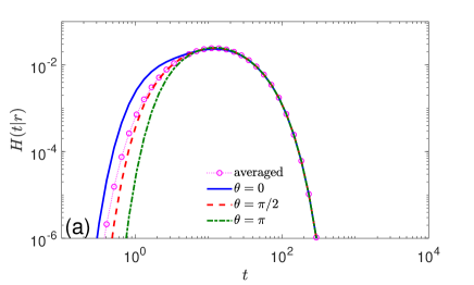
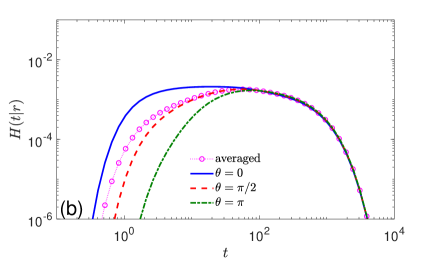
Figure 8: FPT PDF to a circular target located on the North pole of the inner sphere within the ADS, for $R_{1}=1$, $R_{2}=5$, $r=5$, $\varepsilon=0.1$, $D_{s}/D_{b}=1$ (a), and $D_{s}/D_{b}=0.01$ (b). The surface-averaged PDF $\overline{H^{\rm AD}(t;r)}$ (circles) is compared to the PDF $H^{\rm AD}(t;\mathbf{x})$ with a fixed starting point $\mathbf{x}=(r,\theta,0)$, for three choices of $\theta$, as indicated in the legend. All PDFs were obtained via numerical inversion of the Laplace transform by the Talbot algorithm.

Appendix D PDF for one-stage search process

The exact spectral solution for the Laplace-transformed FPT PDF in the conventional one-stage scenario was presented in [50]. This solution involves an infinite-dimensional matrix with explicitly known elements. In practice, one has to truncate this matrix and then numerically invert it.

In order to avoid these numerical steps, we use the self-consistent approximation developed and validated in [50]. The approximate solution reads

$$\tilde{H}_{\rm dir}^{\rm app}(p;\mathbf{x})=J_{p}\sum\limits_{n=0}^{\infty}g_{n}^{(p)}(r)\,P_{n}(\cos\theta)\,\frac{1}{\mu_{n}^{(p)}}\,\frac{P_{n-1}(\cos\varepsilon)-P_{n+1}(\cos\varepsilon)}{2},$$ (112)

where

$$J_{p}=\left(\frac{1}{q}+\frac{1}{2(1-\cos\varepsilon)}\sum\limits_{n=0}^{\infty}\frac{\bigl{(}P_{n-1}(\cos\varepsilon)-P_{n+1}(\cos\varepsilon)\bigr{)}^{2}}{(2n+1)\mu_{n}^{(p)}}\right)^{-1},$$ (113)

and

$$\mu_{n}^{(p)}=-\biggl{(}\frac{\partial g_{n}^{(p)}(r)}{\partial r}\biggr{)}_{r=R_{1}}.$$ (114)

Here, there is no need for matrix inversion as the expression is fully explicit. Moreover, the limit $q\to\infty$ can be easily obtained by simply setting $q=\infty$ in equation (113). While the inverse Laplace transform of equation (112) can be found exactly via the residue theorem (see [50] for details), we resort to a numerical inversion by the Talbot algorithm. When the starting point $\mathbf{x}$ is uniformly distributed over a sphere of radius $r$, equation (112) is reduced to

$$\overline{\tilde{H}_{\rm dir}^{\rm app}(p;r)}=\frac{J_{p}g_{0}^{(p)}(r)}{2\mu_{0}^{(p)}}(1-\cos\varepsilon).$$ (115)

The approximate solution (112) can also be used to compute the moments of the FPT, in particular, the MFPT was derived in Appendix B of [50]. The surface average of equation (B.9) from [50] reads

$$\overline{T_{\rm dir}^{\rm app}}=\frac{R_{2}^{3}-R_{1}^{3}}{3D_{b}R_{1}}\bigg{[}C_{\varepsilon}+\frac{5R_{2}^{3}-9R_{2}^{2}R_{1}+1}{5(R_{2}^{3}-R_{1}^{3})}-R_{1}\frac{5r^{3}+10R_{2}^{3}-3r(R_{1}^{2}+6R_{2}^{2})}{10r(R_{2}^{3}-R_{1}^{3})}\biggr{]},$$ (116)

where

$$C_{\varepsilon}=\frac{2}{(1-\cos\varepsilon)R_{1}q}+\frac{1}{(1-\cos\varepsilon)^{2}}\sum\limits_{n=1}^{\infty}\frac{(P_{n-1}(\cos\varepsilon)-P_{n+1}(\cos\varepsilon))^{2}}{(2n+1)R_{1}\mu_{n}^{(0)}},$$ (117)

and

$$\mu_{n}^{(0)}=\frac{n(n+1)}{R_{1}}\,\frac{1-(R_{1}/R_{2})^{2n+1}}{n+(n+1)(R_{1}/R_{2})^{2n+1}}.$$ (118)

When $R_{1}\ll R_{2}$ the factor $(R_{1}/R_{2})^{2n+1}$ can be neglected, so that $\mu_{n}^{(0)}\approx(n+1)/R_{1}$. The asymptotic behaviour of series like in equation (117) was analysed in [70]. Since $R_{1}\mu_{n}^{(0)}$ can be interpreted as $Rg^{\prime}_{n}(R)/g_{n}(R)$ from the Supplementary Material of [70], one has $1/(R_{1}\mu_{n}^{(0)})\approx 1/(n+1)=1/n-1/n^{2}+O(n^{-3})$ such that one can apply equation (S76) with $\omega=3$ from equation (S56). This yields the small-$\varepsilon$ behaviour

$$C_{\varepsilon}\approx\frac{4}{R_{1}q}\varepsilon^{-2}+\frac{32}{3\pi}\varepsilon^{-1}-\ln(1/\varepsilon)+O(1)\quad(\varepsilon\to 0).$$ (119)

When the target is partially reactive ($q<\infty$) the dominant term scales as $\varepsilon^{-2}$, showing that the direct search is reaction-limited. In turn, for a perfect target, on which we focus in this paper, the first term disappears, and one gets the $\varepsilon^{-1}$-behaviour, with a logarithmic correction. As discussed in [70] for the problem of the narrow escape from a sphere, the numerical factor $32/(3\pi)\approx 3.40$ differs by only $8\%$ from the exact value $\pi$, which was known for that problem. This minor difference comes from the self-consistent approximation. We expect therefore that substitution of $C_{\varepsilon}\approx\pi/\varepsilon$ in equation (116) would result in the correct leading-order behaviour of $\overline{T_{\rm dir}}$ in our setting. In particular, when $\rho\ll R_{1}\ll R_{2}$ (and thus $\varepsilon\ll 1$), we get $\overline{T_{\rm dir}^{\rm app}}\approx\tau_{\rm dir}=R_{2}^{3}/(3D_{b}\rho)$ that was introduced in section 1.

Limit $R_{1}\to R_{2}$

This is an interesting limit in which the thickness of the shell region between the outer and inner spheres shrinks, such that a particle is deemed to perform a diffusive motion almost on the surface of a sphere and seeking a circular target on that surface.

Setting $R_{1}=R-\delta$, $R_{2}=R$ and $r=R$, we get from (114), to the leading order,

$$\mu_{n}^{(p)}\simeq\delta\,\biggl{(}\frac{p}{D}+\frac{n(n+1)}{R^{2}}\biggr{)}+O(\delta^{2}).$$ (120)

In this limit, the self-consistent approximation (112) yields

$$\tilde{H}^{\rm app}_{\rm dir}(p;\mathbf{x}) =(1-\cos\varepsilon)\biggl{(}\sum\limits_{n=0}^{\infty}\frac{(P_{n-1}(\cos\varepsilon)-P_{n+1}(\cos\varepsilon))^{2}}{(2n+1)\bigl{(}\frac{R^{2}p}{D}+n(n+1)\bigr{)}}\biggr{)}^{-1}$$

$$\times\sum\limits_{n=0}^{\infty}\frac{P_{n}(\cos\theta)(P_{n-1}(\cos\varepsilon)-P_{n+1}(\cos\varepsilon))}{\bigl{(}\frac{R^{2}p}{D}+n(n+1)\bigr{)}}.$$ (121)

One can easily check that $\tilde{H}^{\rm app}_{\rm dir}(p;\mathbf{x})$ converges to unity as $p\to 0$, as it should to fulfill the normalisation condition of the PDF. Note that both series can be evaluated explicitly by using the identities (80) and (81).

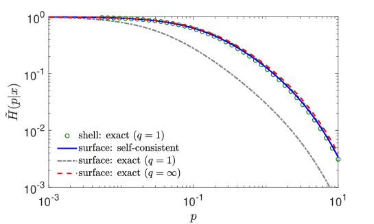
Figure 9: Laplace-transformed PDF $\tilde{H}_{\rm dir}(p;\mathbf{x})$ for diffusion in a thin spherical shell between spheres of radii $R_{1}=0.999$ and $R_{2}=1$ towards a circular target of angular size $\varepsilon=0.1$ located at the North pole, with $r=1$ and $\theta=\pi/2$. Green circles show the exact solution from [50] with $q=1$ (truncated at $n_{\rm max}=100$) and the solid blue line represents equation (121) (the self-consistent approximation in the limit $\delta\to 0$). For comparison, the Laplace-transformed PDF $\tilde{H}^{\rm surf}(p;\theta)$ from equation (72) for surface diffusion with $D_{s}=D_{b}$ towards the same target is shown by the dash-dotted grey line for $q=1$ and by the dashed red line for $q=\infty$.

Curiously, the approximation (121) does not depend on the reactivity parameter $q=\kappa/D_{b}$. This behaviour is illustrated in figure 9, in which we compare the Laplace-transformed PDF for diffusion inside a thin shell (of width $0.001$) to that for surface diffusion on the sphere. There is good agreement between the three curves: the exact solution for a thin shell with $q=1$, the self-consistent approximation (121) (independent of $q$), and the exact solution $\tilde{H}^{\rm surf}(p;\theta)$ from (72) for surface diffusion on the sphere towards a perfectly reactive target ($q=\infty$). In contrast, the exact solution for surface diffusion on the sphere towards a partially reactive target ($q=1$) stands out. We conclude that the Laplace-transformed PDF in a very thin shell is close to that for surface diffusion towards a perfect target.

To rationalise this behaviour, let us consider diffusion in a very thin stripe, $\mathbb{R}\times(0,\delta)$, on which an interval $(-R,R)\times\{0\}$ represents the target. Once a particle enters the proximity of the target (i.e., the rectangle $(-R,R)\times(0,\delta)$), it hits the target a very large number of times, so that the reaction occurs very rapidly after entering this zone. In the limit $\delta\to 0$, the number of encounters grows, such that the effective target on the line is perfectly reactive. The same argument holds for three-dimensional diffusion between parallel planes, $\mathbb{R}^{2}\times(0,\delta)$, when the target is a disk $\{(x,y,0)\in\mathbb{R}^{3}:x^{2}+y^{2}<R^{2}\}$. This is equivalent to our setting because the curvature of the spherical shell does not matter in the limit $\delta\to 0$.

Numerical implementation

Even though the approximative solution (112) is fully explicit, its numerical computation may be challenging, especially for small $\varepsilon$. In fact, one needs to truncate the infinite series in (113), and the truncation order $n_{\rm max}$ has to be large when $\varepsilon$ is small. At the same time, the numerical evaluation of the radial function $g_{n}^{(p)}$ that involve $i_{n}(z)$ and $k_{n}(z)$ and determine $\mu_{n}^{(p)}$, becomes unstable for large $n$. Moreover, as one needs to perform an inverse Laplace transform of $\tilde{H}_{\rm dir}^{\rm app}(p;\mathbf{x})$ to get back to the time domain, this computation has to be realised for any $p\in\mathbb{C}$. In order to overcome these numerical difficulties, we adopt the following two-step scheme.

In the first step, we approximate the radial functions with large $n$ as

$$g_{n}^{(p)}(r)\approx g_{n,\infty}^{(p)}(r)=\frac{k_{n}(\alpha r)}{k_{n}(\alpha R_{1})},$$ (122)

where $\alpha=\sqrt{p/D}$ and $g_{n,\infty}^{(p)}(r)$ are the radial functions for the problem without outer sphere (i.e., for $R_{2}=\infty$). This approximation can be easily justified in the limit $p\to\infty$ for any $r<R_{2}$ and any $n$ just by looking at the asymptotic behaviour of the modified spherical Bessel functions $i_{n}(z)$ and $k_{n}(z)$ in (7). We checked numerically that this approximation is also applicable for smaller $p$ if $r\ll R_{2}$ and $n\gg 1$.

In the second step, we employ the recurrence relations for $k_{n}(z)$ to enable an iterative computation of the radial function. In fact, one has

$$k_{n+1}(z)=k_{n-1}(z)+\frac{2n+1}{z}k_{n}(z),\qquad k^{\prime}_{n}(z)=-k_{n-1}(z)-\frac{n+1}{z}k_{n}(z).$$ (123)

Using the first relation, one gets

$$g_{n+1,\infty}^{(p)}(r)=\frac{k_{n-1}(\alpha r)+\frac{2n+1}{\alpha r}k_{n}(\alpha r)}{k_{n-1}(\alpha R_{1})+\frac{2n+1}{\alpha R_{1}}k_{n}(\alpha R_{1})}=g_{n,\infty}^{(p)}(r)\frac{R_{1}}{r}\frac{1+\frac{f_{n}(\alpha r)}{2n+1}}{1+\frac{f_{n}(\alpha R_{1})}{2n+1}},$$ (124)

where

$$f_{n}(z)=z\frac{k_{n-1}(z)}{k_{n}(z)}.$$ (125)

Using again the first recurrence relation and the explicit form $k_{0}(z)=e^{-z}/z$ one finds

$$f_{1}(z)=\frac{z^{2}}{z+1},\qquad f_{n}(z)=\frac{z^{2}}{f_{n-1}(z)+2n-1}\quad(n=2,3,\ldots).$$ (126)

One sees that the $f_{n}(z)$ are rational functions, which can be computed iteratively. These functions have the following asymptotic behaviours

$$f_{n}(z)\simeq\frac{z^{2}}{2n-1}-\frac{z^{4}}{(2n-1)^{2}(2n-3)}+O(z^{6})\quad(z\to 0)$$ (127)

for $n>1$ (note that $f_{1}(z)=z^{2}-z^{3}+\ldots$ contains the $z^{3}$ term), and

$$f_{n}(z)\simeq z-n+\frac{n(n+1)}{2z}+O(z^{-2})\quad(z\to\infty).$$ (128)

Finally, we can approximate

$$\mu_{n}^{(p)}\approx\mu_{n,\infty}^{(p)}=-\biggl{(}\partial_{r}g_{n,\infty}^{(p)}(r)\biggr{)}_{r=R_{1}}=-\alpha\frac{k^{\prime}_{n}(\alpha R_{1})}{k_{n}(\alpha R_{1})}.$$ (129)

Using the second recurrence relation, one then gets

$$R_{1}\mu_{n,\infty}^{(p)}=n+1+f_{n}(\alpha R_{1})\qquad(n=1,2,\ldots)$$ (130)

(note that $R_{1}\mu_{0,\infty}^{(p)}=1+\alpha R_{1}$). We then use the following numerical approximation

$$J_{p} \approx\left(\frac{1}{q}+\frac{1}{2(1-\cos\varepsilon)}\left\{\sum\limits_{n=0}^{n_{\rm app}}\frac{\bigl{(}P_{n-1}(\cos\varepsilon)-P_{n+1}(\cos\varepsilon)\bigr{)}^{2}}{(2n+1)\mu_{n}^{(p)}}\right.\right.$$

$$\left.\left.+\sum\limits_{n=n_{\rm app}+1}^{n_{\rm max}}\frac{\bigl{(}P_{n-1}(\cos\varepsilon)-P_{n+1}(\cos\varepsilon)\bigr{)}^{2}}{(2n+1)\mu_{n,\infty}^{(p)}}\right\}\right)^{-1},$$ (131)

in which we keep the first $n_{\rm app}+1$ terms with the exact form of $\mu_{n}^{(p)}$ and replace $\mu_{n}^{(p)}$ by its approximation $\mu_{n,\infty}^{(p)}$ from (130) for the terms with $n_{\rm app}<n\leq n_{\rm max}$. In this way, the truncation order $n_{\rm max}$ can be made sufficiently large to ensure accurate computations. We used $n_{\rm app}=50$ and $n_{\rm max}=250$.

References

References

- [1] G. Adam and M. Delbrück, Reduction of Dimensionality in Biological Diffusion Processes, In Structural Chemistry and Molecular Biology, A. Rich and N. Davidson, Eds. (W H Freeman and Co., San Francisco, 1968).
- [2] H. J. Trurnit, Über monomolekulare Filme an Wassergrenzflächen und über Schichtfilme, In: Fortschritte der Chemie Organischer Naturstoffe, vol 4., A. Butenandt et al. (eds) (Springer, Vienna, 1945).
- [3] T. Bücher, Probleme des Energietransports innerhalb lebender Zellen, Adv. Enzymol. 14, 1 (1953).
- [4] M. Eigen, Diffusion control in biochemical reactions, in Quantum Statistical Mechanics in the Natural Sciences, S. L. Mintz and S. N. Widmayer, eds. (Plenum Press, New York, 1974), p. 37
- [5] P. M. Richter and M. Eigen, Diffusion controlled reaction rates in spheroidal geometry. Application to repressor-operator association and membrane bound enzymes, Biophys. Chem. 2, 255 (1974).
- [6] A. J. Frank, M. Grätzel and J. J. Kozak, On the reduction of dimensionality in radical decay kinetics induced by micellar systems, J. Am. Chem. Soc. 98, 3317 (1976).
- [7] H. C. Berg and E. M. Purcell, Physics of Chemoreception, Biophys. J. 20, 193 (1977).
- [8] R. D. Astumian and Z. A. Schelly, Geometric effects of reduction of dimensionality in interfacial reactions, J. Am. Chem. Soc. 106, 304 (1984).
- [9] P. H. Lee and J. J. Kozak, Lattice theory of reaction efficiency in compartmentalized systems. II. Reduction of dimensionality, J. Chem. Phys. 80, 705 (1984).
- [10] D. Shoup, G. Lipari and A. Szabo, Diffusion-controlled bimolecular reaction rates. The effect of rotational diffusion and orientation constraints, Biophys. J. 36, 697 (1981).
- [11] R. Zwanzig and A. Szabo, Time dependent rate of diffusion influenced ligand binding to receptors on cell surfaces, Biophys. J. 60, 671 (1991).
- [12] D. Axelrod and M. D. Wang, Reduction-of-Dimensionality Kinetics at Reaction-Limited Cell Surface Receptors, Biophys. J. 66, 588 (1994).
- [13] M. Schmick and P. I. H. Bastiaens, The Interdependence of Membrane Shape and Cellular Signal Processing, Cell 156, 1132 (2014).
- [14] M. A. McCloskey and M-m Poo, Rates of Membrane-associated Reactions: Reduction of Dimensionality Revisited, J. Cell Biology 102, 88 (1986).
- [15] O. G. Berg, R. B. Winter and P. H. von Hippel, Diffusion-driven mechanisms of protein translocation on nucleic acids. 1. Models and theory, Biochemistry 20, 6929 (1981).
- [16] P. H. von Hippel and O. G. Berg, Facilitated target location in biological systems, J. Biol. Chem. 264, 675 (1989).
- [17] M. Coppey, O. Bénichou, R. Voituriez and M. Moreau, Kinetics of Target Site Localization of a Protein on DNA: A Stochastic Approach, Biophys. J. 87, 1640 (2004).
- [18] S. E. Halford and J. F. Marko, How do site-specific DNA-binding proteins find their targets?, Nucleic Acids Res. 32, 3040 (2004).
- [19] T. Hu, A. Y. Grosberg and B. I. Shklovskii, How Proteins Search for Their Specific Sites on DNA: The Role of DNA Conformation, Biophys. J. 90, 2731 (2006).
- [20] L. Mirny, Cell commuters avoid delays, Nature Phys. 4, 93 (2008).
- [21] L. Mirny, M. Slutsky, Z. Wunderlich, A. Tafvizi, J. Leith, and A. Kosmrlj, How a protein searches for its site on DNA: the mechanism of facilitated diffusion, J. Phys. A: Math. Theor. 42, 434013 (2009).
- [22] M. A. Lomholt, B. van den Broek, S-M. J. Kalisc, G. J. L. Wuite and R. Metzler, Facilitated diffusion with DNA coiling, Proc. Natl. Acad. Sci. USA 106, 8204 (2009).
- [23] B. van den Broek, M. A. Lomholt, S.-M. J. Kalisch, R. Metzler, and G. J. L. Wuite, How DNA coiling enhances target localization by proteins, Proc. Natl. Acad. Sci. USA 105, 15738 (2008).
- [24] K. V. Klenin, H. Merlitz, J. Langowski, and C.-X. Wu, Facilitated Diffusion of DNA-Binding Proteins, Phys. Rev. Lett. 96, 018104 (2006).
- [25] G. Kolesov, Z. Wunderlich, O. N. Laikova, M. S. Gelfand, and L. A. Mirny, How gene order is influenced by the biophysics of transcription regulation, Proc. Natl. Acad. Sci. USA 104, 13948 (2007).
- [26] O. Pulkkinen and R. Metzler, Distance matters: the impact of gene proximity in bacterial gene regulation, Phys. Rev. Lett. 110, 198101 (2013).
- [27] M. Slutsky and L. A. Mirny, Kinetics of Protein-DNA Interaction: Facilitated Target Location in Sequence-Dependent Potential, Biophys. J. 87, 4021 (2004).
- [28] M. Bauer and R. Metzler, In vivo facilitated diffusion model, PLoS ONE 8, e53956 (2013).
- [29] M. Sheinman, O. Bénichou, Y. Kafri and R. Voituriez, Classes of fast and specific search mechanisms for proteins on DNA, Rep. Prog. Phys. 75, 026601 (2012).
-
[30]
R. Peters, Translocation through the nuclear pore
complex: Selectivity and speed by reduction-of-dimensionality, Traffic
6, 421 (2005)
Translocation through the nuclear pore: Kaps pave the way, BioEssays 31, 466 (2009). - [31] O. Bénichou, M. Coppey, M. Moreau, P-H. Suet, and R. Voituriez, Optimal Search Strategies for Hidden Targets, Phys. Rev. Lett.94, 198101 (2005).
- [32] O. Bénichou, C. Loverdo, M. Moreau, and R. Voituriez, Intermittent search strategies, Rev. Mod. Phys. 83, 81 (2011).
- [33] O. Bénichou, D. S. Grebenkov, P. Levitz, C. Loverdo, and R. Voituriez, Optimal Reaction Time for Surface-Mediated Diffusion, Phys. Rev. Lett. 105, 150606 (2010).
- [34] O. Bénichou, D. S. Grebenkov, P. Levitz, C. Loverdo, and R. Voituriez, Mean First-Passage Time of Surface-Mediated Diffusion in Spherical Domains, J. Stat. Phys. 142, 657-685 (2011).
- [35] J.-F. Rupprecht, O. Bénichou, D. S. Grebenkov, and R. Voituriez, Kinetics of Active Surface-Mediated Diffusion in Spherically Symmetric Domains, J. Stat. Phys. 147, 891-918 (2012).
- [36] J.-F. Rupprecht, O. Bénichou, D. S. Grebenkov, and R. Voituriez, Exact mean exit time for surface-mediated diffusion, Phys. Rev. E 86, 041135 (2012).
- [37] F. Rojo and C. E. Budde, Enhanced diffusion through surface excursion: A master-equation approach to the narrow-escape-time problem, Phys. Rev. E 84, 021117 (2011).
- [38] F. Rojo, C. E. Budde Jr., H. S. Wio, and C. E. Budde, Enhanced transport through desorption-mediated diffusion, Phys. Rev. E 87, 012115 (2013).
- [39] O. Bénichou, D. S. Grebenkov, L. Hillairet, L. Phun, R. Voituriez, and M. Zinsmeister, Mean exit time for surface-mediated diffusion: spectral analysis and asymptotic behavior, Anal. Math. Phys. (2015).
- [40] M. A. Lomholt, T. Koren, R. Metzler, and J. Klafter, Lévy strategies in intermittent search processes are advantageous, Proc. Natl. Acad. Sci. USA 105, 11055 (2008).
- [41] G. Oshanin, M. Tamm and O. Vasilyev, Narrow-escape times for diffusion in microdomains with a particle-surface affinity: mean-field results, J. Chem. Phys. 132, 06B607 (2010).
- [42] G. Oshanin, H. S. Wio, K Lindenberg, and S. F. Burlatsky, Intermittent random walks for an optimal search strategy: one-dimensional case, J. Phys.: Condens. Matt. 19, 065142 (2007).
- [43] G. Oshanin, K. Lindenberg, H. S. Wio, and S. Burlatsky, Efficient search by optimized intermittent random walks, J. Phys. A: Math. and Theor. 42, 434008 (2009).
- [44] F. Rojo, J. Revelli, C. E. Budde, H. S. Wio, G. Oshanin, and K. Lindenberg, Intermittent search strategies revisited: effect of the jump length and biased motion, J. Phys. A: Math. and Theor. 43, 345001 (2010).
- [45] V. V. Palyulin, A. V. Chechkin, and R. Metzler, Lévy flights do not always optimize random blind search for sparse targets, Proc. Natl. Acad. Sci. USA 111, 2931 (2014).
- [46] V. Palyulin, A. V. Chechkin, R. Klages, and R. Metzler, Search reliability and search efficiency of combined Lévy-Brownian motion: long relocations mingled with thorough local exploration, J. Phys. A 49, 394002 (2016).
- [47] O. Bénichou and R. Voituriez, From first-passage times of random walks in confinement to geometry-controlled kinetics, Phys. Rep. 539, 225 (2014).
- [48] S. Redner, A Guide to First Passage Processes (Cambridge: Cambridge University Press, 2001).
- [49] R. Metzler, G. Oshanin and S. Redner, eds., First-passage phenomena and their applications (World Scientific Publishers: Singapore, 2014).
- [50] D. S. Grebenkov, R. Metzler, and G. Oshanin, Distribution of first-reaction times with target sites on boundaries of shell-like regions, New J. Phys. 23, 123049 (2021).
- [51] S. R. McGuffee and A. H. Elcock, Diffusion, Crowding and Protein Stability in a Dynamic Molecular Model of the Bacterial Cytoplasm, PLoS ComputBiol 6, e1000694 (2010).
- [52] S. K. Ghosh, A. G. Cherstvy, D. S. Grebenkov, and R. Metzler, Anomalous, non-Gaussian tracer diffusion in heterogeneously crowded environments, New J. Phys. 18, 013027 (2016).
- [53] J. Ma, M. Do, M. A. Le Gros, C. S. Peskin, C. A. Larabell, Y. Mori, and S. A. Isaacson, Strong intracellular signal inactivation produces sharper and more robust signaling from cell membrane to nucleus, PLoS Comput. Biol. 16, e1008356 (2020).
- [54] E. R. Weikum, X. Liu, and E. A. Ortlund, The nuclear receptor superfamily: A structural perspective, Protein Sci. 27, 1876 (2018).
- [55] G. Antczak and G. Ehrlich, Jump processes in surface diffusion, Surface Science Rep. 62, 39 (2007).
- [56] M. D. Huber and L. Gerace, The size-wise nucleus: nuclear volume control in eukaryotes, J. Cell Biol. 179, 583 (2007).
- [57] A. Rizzotto and E. C. Schirmer, Breaking the scale: how disrupting the karyoplasmic ratio gives cancer cells an advantage for metastatic invasion, Biochem. Soc. Trans. 45, 1333 (2017).
- [58] M. E. Malerba and D. J. Marshall, Larger cells have relatively smaller nuclei across the Tree of Life, Evol. Lett. 5, 306 (2021).
- [59] E. W. Sinnott and V. V. Trombetta, The cytonuclear ratio in plant cells, Am. J. Botany 23, 602 (1936).
- [60] C. Mejía-Monasterio, G. Oshanin and G. Schehr, First passages for a search by a swarm of independent random searchers, J. Stat. Mech. P06022 (2011).
- [61] T. G. Mattos, C. Mejía-Monasterio, R. Metzler, and G. Oshanin, First passages in bounded domains: When is the mean first passage time meaningful? Phys. Rev. E 86 031143 (2012).
- [62] A. Godec and R. Metzler, Optimization and universality of Brownian search in quenched heterogeneous media, Phys. Rev. E 91, 052134 (2015).
- [63] A. Godec and R. Metzler, Universal proximity effect in target search kinetics in the few encounter limit, Phys. Rev. X 6, 041037 (2016).
- [64] D. S. Grebenkov, R. Metzler and G. Oshanin, Strong defocusing of molecular reaction times results from an interplay of geometry and reaction control, Comm. Chem. 1, 96 (2018).
- [65] D. S. Grebenkov, R. Metzler and G. Oshanin, Towards a full quantitative description of single-molecule reaction kinetics in biological cells, Phys. Chem. Chem. Phys. 20, 16393 (2018).
- [66] D. S. Grebenkov, R. Metzler and G. Oshanin, Full distribution of first exit times in the narrow escape problem, New J. Phys. 21, 122001 (2019).
- [67] D. S. Grebenkov, Paradigm Shift in Diffusion-Mediated Surface Phenomena, Phys. Rev. Lett. 125, 078102 (2020).
- [68] D. S. Grebenkov, Joint distribution of multiple boundary local times and related first-passage time problems with multiple targets, J. Stat. Mech. 103205 (2020)
- [69] D. S. Grebenkov, An encounter-based approach for restricted diffusion with a gradient drift, J. Phys. A: Math. Theor. 55, 045203 (2022).
- [70] D. S. Grebenkov and G. Oshanin, Diffusive escape through a narrow opening: new insights into a classic problem, Phys. Chem. Chem. Phys. 19, 2723 (2017).
- [71] G. Oshanin, M. N. Popescu and S. Dietrich, Active colloids in the context of chemical kinetics, J. Phys. A: Math. Theor. 50, 134001 (2017).
- [72] D. S. Grebenkov, R. Metzler, and G. Oshanin, Effects of the target aspect ratio and intrinsic reactivity onto diffusive search in bounded domains, New J. Phys. 19, 103025 (2017).
- [73] D. Purves et al, eds., Neuroscience, 2nd ed. (Sunderland (MA): Sinauer Associates, 2001).
- [74] B. Alberts et al, Molecular Biology of the Cell, th ed. (New York: Garland, 2015).
- [75] D. S. Grebenkov, R. Metzler, and G. Oshanin, A molecular relay race: sequential first-passage events to the terminal reaction centre in a cascade of diffusion controlled processes, New J. Phys. 23, 093004 (2021).
- [76] D. S. Grebenkov, Surface Hopping Propagator: An Alternative Approach to Diffusion-Influenced Reactions, Phys. Rev. E 102, 032125 (2020).
- [77] N. Chao, S. H. Young and M. Poo, Localization of cell membrane components by surface diffusion into a trap, Biophys. J. 36, 139 (1981).
- [78] H. Sano and M. Tachiya, Theory of diffusion-controlled reactions on spherical surfaces and its application to reactions on micellar surfaces, J. Chem. Phys. 75, 2870 (1981).
- [79] T. Prüstel and M. Tachiya, Reversible diffusion-influenced reactions of an isolated pair on some two dimensional surfaces, J. Chem. Phys. 139, 194103 (2013).
- [80] D. S. Grebenkov, Reversible reactions controlled by surface diffusion on a sphere, J. Chem. Phys. 151, 154103 (2019).
- [81] S. N. Majumdar and B. Meerson, Statistics of first-passage Brownian functionals, J. Stat. Mech. (2020) 023202; Corrigendum: J. Stat. Mech. (2021) 039801.
- [82] B. Meerson and N. R. Smith, Geometrical optics of constrained Brownian motion: three short stories, J. Phys. A: Math. Theor. 52, 415001 (2019).
- [83] C. Antoine and J. Talbot, Enhancing search efficiency through diffusive echo (submitted; E-print: arXiv:2205.09942v1).
- [84] G. H. Weiss, K. E. Shuler, and K. Lindenberg, Order Statistics for First Passage Times in Diffusion Processes, J. Stat. Phys. 31, 255 (1983).
- [85] K. Basnayake, A. Hubl, Z. Schuss, and D. Holcman, Extreme narrow escape: Shortest paths for the first particles among n to reach a target window, Phys. Lett. A 382, 3449 (2018).
- [86] K. Basnayake, Z. Schuss, and D. Holcman, Asymptotic formulas for extreme statistics of escape times in 1, 2 and 3-dimensions, J. Nonlinear Sci. 29, 461-499 (2019).
- [87] Z. Schuss, K. Basnayake, and D. Holcman, Redundancy principle and the role of extreme statistics in molecular and cellular biology, Phys. Life Rev. 28, 52-79 (2019).
- [88] D. S. Lawley and J. B. Madrid, A Probabilistic Approach to Extreme Statistics of Brownian Escape Times in Dimensions 1, 2, and 3, J. Nonlinear Sci. 30, 1207-1227 (2020).
- [89] D. S. Lawley, Distribution of extreme first passage times of diffusion, J. Math. Biol. 80, 2301 (2020).
- [90] D. S. Grebenkov, R. Metzler, and G. Oshanin, From single-particle stochastic kinetics to macroscopic reaction rates: fastest first-passage time of N random walkers, New J. Phys. 22, 103004 (2020).
- [91] S. N. Majumdar, A. Pal, and G. Schehr, Extreme value statistics of correlated random variables: a pedagogical review, Phys. Rep. 840, 1 (2020).
- [92] D. S. Grebenkov, Depletion of Resources by a Population of Diffusing Species, Phys. Rev. E 105, 054402 (2022).
- [93] J. F. Reverey, J.-H. Jeon, H. Bao, M. Leippe, R. Metzler, and C. Selhuber-Unkel, Superdiffusion dominates intracellular particle motion in the supercrowded space of pathogenic Acanthamoeba castellanii, Sci. Rep. 5, 11690 (2015).
- [94] S. Thapa, N. Lukat, C. Selhuber-Unkel, A. Cherstvy, and R. Metzler, Transient superdiffusion of polydisperse vacuoles in highly-motile amoeboid cells, J. Chem. Phys. 150, 144901 (2019).
- [95] P. Witzel, M. Götz, Y. Lanoiselée, T. Franosch, D. S. Grebenkov, and D. Heinrich, Heterogeneities Shape Passive Intracellular Transport, Biophys. J. 117, 203-213 (2019).
- [96] A. V. Chechkin, F. Seno, R. Metzler, and I. M. Sokolov, Brownian yet Non-Gaussian Diffusion: From Superstatistics to Subordination of Diffusing Diffusivities, Phys. Rev. X 7, 021002 (2017).
- [97] Y. Lanoiselée, N. Moutal, and D. S. Grebenkov, Diffusion-limited reactions in dynamic heterogeneous media, Nature Commun. 9, 4398 (2018).
- [98] D. S. Grebenkov, A physicist’s guide to explicit summation formulas involving zeros of Bessel functions and related spectral sums, Rev. Math. Phys. 33, 2130002 (2021).
- [99] A. Erdélyi, Higher transcendental functions, vol. 1. (Robert E. Krieger Publishing, Malabar FL, 1953).
- [100] R. Szmytkowski, The parameter derivatives and , where is the Legendre function of the first kind, E-print arXiv:1301.6586 (2013).
- [101] B. J. Laurenzi, Derivatives with respect to the order of the Legendre Polynomials, E-print arXiv:1502.06507v1 (2015).