Estimation of Predictive Performance in High-Dimensional Data Settings using Learning Curves

Abstract

In high-dimensional prediction settings, it remains challenging to reliably estimate the test performance. To address this challenge, a novel performance estimation framework is presented. This framework, called Learn2Evaluate, is based on learning curves by fitting a smooth monotone curve depicting test performance as a function of the sample size. Learn2Evaluate has several advantages compared to commonly applied performance estimation methodologies. Firstly, a learning curve offers a graphical overview of a learner. This overview assists in assessing the potential benefit of adding training samples and it provides a more complete comparison between learners than performance estimates at a fixed subsample size. Secondly, a learning curve facilitates in estimating the performance at the total sample size rather than a subsample size. Thirdly, Learn2Evaluate allows the computation of a theoretically justified and useful lower confidence bound. Furthermore, this bound may be tightened by performing a bias correction. The benefits of Learn2Evaluate are illustrated by a simulation study and applications to omics data.

Keywords: High-dimensional data, Omics, Predictive performance, Area under the receiver operating curve, Bootstrap, Cross-validation

1 Introduction

Nowadays, many learners can predict a response from high-dimensional data. To select the most accurate learner, it is key to reliably estimate the predictive performance with a confidence bound. The predictive performance may be quantified by many different metrics. For classification, examples include the accuracy, the area under the receiver operating curve (AUC) [Hanley and McNeil, 1982], and the brier score [Brier, 1950], whereas for regression one usually reports the mean square error of prediction (PMSE).

It is well-known that performance estimates are optimistically biased when they are based on the same data used to fit the learner. This optimism bias is even more apparent for high-dimensional learners, as such learners overfit quickly. Performance estimates should therefore be based on independent test data. However, for many high-dimensional prediction studies, a test set is unavailable. Therefore, learning the model and estimating the performance should be based on a single, often small-sized, data set. In this paper, we present a novel methodology to estimate the predictive performance in such a scenario.

The standard method for performance estimation in small sample size settings is resampling such as repeated hold-out [Burman, 1989], K-fold cross-validation [Stone, 1974], or bootstrapping [Efron and Tibshirani, 1994]. These techniques repeatedly partition or resample the available data in a training set of a fixed size, to fit the model, and a test set, to estimate the performance. An acknowledged challenge for these techniques is to choose the size of the training sets. Training sets that are close in size to the complete data set lead to an almost unbiased predictive performance estimate. However, such training sets also induce a large variability of the performance estimate because the test sets are small. Resampling techniques are, therefore, faced with a bias-variance trade-off, which leads to conservative and often useless confidence bounds for the performance. Advances in these techniques improve the uncertainty estimates [Michiels et al., 2005, Jiang et al., 2008], but neither provide a theoretical justification nor a point estimate.

Another performance estimation strategy is to combine resampling with an asymptotic or parametric method to construct a confidence bound. For the cross-validated AUC, a confidence bound based on influence functions was derived [LeDell et al., 2015], and Monte Carlo simulation was combined with a parametric model to construct a confidence bound for the cross-validated accuracy [Dobbin, 2009]. However, the former bound is too liberal for small sample sizes and the latter method only applies to linear learners. Moreover, both methods lack generality because they only apply to a specific predictive performance metric.

To address the aforementioned issues, we present Learn2Evaluate, a learning-curve-based performance estimation framework. A learning curve combines resampling with smoothing by fitting a monotone curve depicting the predictive performance on left-out samples as a function of the size of the training set [Cortes et al., 1993, Mukherjee et al., 2003]. The learning curve enables us to obtain a point estimate of the performance at the full sample size and to determine an optimal training set size to construct a conservative confidence bound. Additionally, this bound can be tightened by performing a bias correction. The idea of finding an optimal training set size builds on previous work by Dobbin and Simon [2011]. They employed learning curves to find a good training set size in single split sample approach. In contrast, we consider multiple splits into a training and test set, and we focus on a confidence bound.

Learn2Evaluate has several advantages compared to other performance estimation techniques. Firstly, Learn2Evaluate is generic and applies to any learner and any performance metric. Secondly, it renders a point estimate and a confidence bound. Importantly, this confidence bound is theoretically justified, as we will prove type-I error control, and it explicitly takes the size of the training set into account.

In addition, because Learn2Evaluate is based on learning curves, it automatically offers a graphical technique to study several aspects of a learner. Firstly, the slope of the curve at the total sample size allows a qualitative assessment of the benefit of future samples. Secondly, learning curves provide a more complete comparison between different learners than just performance point estimates at a fixed training set size. Lastly, one may observe that prediction models learn at different rates, which could lead to a deeper understanding of learning behaviors.

The remainder of this paper is organized as follows. In Section 2, we describe Learn2Evaluate and provide a theoretical justification for the confidence bound. We present simulation results in Section 3 and in Section 4, we illustrate the benefits of Learn2Evaluate on omics data. We end with some conclusive remarks in Section 5.

2 Methods

2.1 Target parameter

Let our data $D=\left\{\left(\boldsymbol{X}_{i},Y_{i}\right)\right\}_{i=1}^{N}$ consist of $N$ observations of a $p$-dimensional feature vector $\boldsymbol{X}_{i}$ with a corresponding response variable $Y_{i}.$ The goal in prediction problems is to fit a learner $\varphi_{D}$ on data $D$ that reliably predicts $Y$ from $\boldsymbol{X}.$ After learner $\varphi_{D}$ is fitted, we wish to evaluate the predictive performance $\rho_{D},$ i.e. the quality of predictions of $\varphi_{D}$ of yet unseen data points. Subscript $D$ indicates that $\rho_{D}$ is conditional on the data $D.$

2.2 Predictive performance estimation

To evaluate $\rho_{D},$ we report a point estimate $\hat{\rho}_{D}$ and a lower confidence bound $L_{D}\left(\alpha\right)$ for $\rho_{D}$ that satisfies $P\left(L_{D}\left(\alpha\right)\leq\rho_{D}\right)\geq 1-\alpha.$ We consider the case where a large test data set is not available. Learning $\varphi_{D}$ and estimating $\hat{\rho}_{D}$ and $L_{D}\left(\alpha\right)$ should therefore be solely based on data $D$.

To use $D$ efficiently, one may apply resampling techniques. These techniques create multiple training sets, on which $\varphi$ is learned, and complementary test sets, on which the estimates $\hat{\rho}_{D}$ and $L_{D}\left(\alpha\right)$ are based. Since $\varphi$ is now learned on a subset of $D,$ it is more difficult to find the structure in $\boldsymbol{X}$ that explains $Y.$ This often leads to a pessimistically biased estimate of $\rho_{D}.$ Larger training sets reduce this bias, but also lead to smaller test sets, which in turn increases the variance of the performance estimate. Resampling-based estimators are therefore faced with a bias-variance trade-off. This trade-off makes it particularly difficult to obtain a practical confidence bound as such a bound depends on both the bias and the variance.

To address the bias-variance trade-off, we present a novel learning-curve-based performance estimation method. In the following, we formally define the learning curve and discuss how we use it for predictive performance estimation. Here, we distinguish between increasing performance metrics such as the AUC, which are metrics that increase when more signal is captured, and decreasing performance metrics such as the PMSE. Our method is presented for the AUC because classification is a frequent application in high-dimensional and small sample size settings. Extending our method to decreasing performance metrics is straightforward and is explained for the PMSE. Our method, which we call Learn2Evaluate, is summarized in Figure 1.

2.3 Definition of the learning curve

A learning curve is constructed by first applying repeated hold-out estimation for several training set sizes, followed by a smoothing step.

2.3.1 Repeated hold-out estimation

To define repeated hold-out estimation, we first introduce single hold-out estimation. Let $s_{n}^{k}$ be the $k\mbox{th}$ realization of a random subset of $D$ with size $n\leq N$. This subset is taken without replacement and is balanced with respect to the response if $Y$ is binary. For continuous $Y,$ we do not impose the balancing restriction. We then define $\rho_{s_{n}^{k}}$ as the predictive performance when $s_{n}^{k}$ is used to build a learner $\varphi_{s_{n}^{k}}$. We estimate $\rho_{s_{n}^{k}}$ based on the complement or hold-out set $D\setminus s_{n}^{k}.$ This yields the single hold-out performance estimate $\hat{\rho}_{s_{n}^{k}}$ and a lower confidence bound $L_{s_{n}^{k}}(\alpha).$ We assume that a method to construct $L_{s_{n}^{k}}(\alpha)$ exists. For the AUC, we employ the nonparametric method of DeLong et al. [1988] implemented in the R package pROC [Robin et al., 2011]. For decreasing performance metrics, such as the PMSE, we estimate an upper confidence bound.

The single hold-out estimate depends on the subset $s_{n}^{k}$. To reduce this dependency, we apply repeated hold-out estimation. We define $\rho_{n}$ as the average performance over all $V$ possible subsets of $D$ of size $n\leq N,$

$$\rho_{n}=\frac{1}{V}\sum_{k=1}^{V}\rho_{s_{n}^{k}},$$

with $V=\binom{N}{n}$ for unrestricted sampling, and $V=\binom{N_{+}}{n_{+}}\binom{N_{-}}{n_{-}}$ for balanced sampling, with subscript $+/-$ denoting the number of positive/negative cases of the given (sub)sample size. The average performance is estimated by the repeated hold-out estimate $\hat{\rho}_{n}$, which is based on $K\leq V$ subsets,

$$\hat{\rho}_{n}=\frac{1}{K}\sum_{k=1}^{K}\hat{\rho}_{s_{n}^{k}}.$$ (1)

Repeated hold-out estimation also yields $K$ lower confidence bounds $L_{s_{n}^{k}}.$ In Theorem 1, we prove how to aggregate these bounds to obtain a $(1-\alpha)$ confidence bound for $\rho_{D}.$

Conventional repeated hold-out estimation uses (1) as a point estimate for the performance $\rho_{D}.$ A learning curve, however, relies on first evaluating (1) for a sequence of $J$ subsample sizes $n_{1}<\ldots<n_{J}$, yielding a learning trajectory (Figure 1, black dots),

$$\left\{(n_{j},\hat{\rho}_{n_{j}})\right\}_{j=1}^{J}.$$ (2)

The learning curve is then obtained by smoothing this trajectory and the fit provides an estimate of $\rho_{D}.$

2.3.2 Smoothing

A learning curve $f(n)$ (Figure 1, solid purple line) is a fit of the learning trajectory, i.e. (2), rendering a relationship between the subsample size and the predictive performance. We assume that this relationship is monotonically increasing,

$$\forall j>0:\,\rho_{n_{j}}\leq\rho_{n_{j+1}}.$$ (3)

Assumption (3) is a natural one: the average performance of a learner trained on larger subsets is likely higher than that of the same learner trained on smaller subsets.

In addition, we assume that the learning curve is concave after some threshold subsample size $n_{tr}$, $\forall n_{j}\geq n_{tr},j>0:\,\left(\rho_{n_{j+2}}-\rho_{n_{j+1}}\right)/\left(n_{j+2}-n_{j+1}\right)\leq\left(\rho_{n_{j+1}}-\rho_{n_{j}}\right)/\left(n_{j+1}-n_{j}\right).$ This assumption is employed to stabilize the curve. In some situations, the concavity assumption may not hold for the considered trajectory of subsample sizes, i.e. $n_{1}\leq n_{tr}.$ This can be assessed visually from the learning trajectory. For example, in some situations, lasso regression is known to exhibit a phase transition [Donoho and Tanner, 2005], which would lead to a S-shaped learning curve. For such an instance, we propose to first determine $n_{tr}$, i.e. the inflection point of the S-shaped curve, followed by fitting a learning curve with smallest subsample size $n_{1}=n_{tr}.$ In supplementary Section 1, we show a method to determine $n_{tr}.$ Note that the case $n_{J}\leq n_{tr}$ is a strong indication for acquiring more samples before developing a learner.

For decreasing performance metrics, the assumptions should be reversed, leading to a monotonically decreasing and convex curve.

To fit the learning curve, we consider a parametric model, based on an inverse power law, and a nonparametric model, based on a constrained regression spline. Use of power laws for fitting learning curves has been empirically established [Cortes et al., 1993, Mukherjee et al., 2003, Hess and Wei, 2010]. We examine constrained regression splines because they do not rely on a specific shape of $f,$ while the constraints prevent a too flexible fit.

Inverse power law

To fit an inverse power law, we perform nonlinear least squares regression, with

$$f(n)=\delta-\beta n^{-\gamma}.$$ (4)

This function grows, with increasing subsample size $n$, asymptotically to parameter $\delta$, with $0.5\leq\delta\leq 1$ for the AUC. The learning rate $\beta$ and the decay rate $\gamma$ are positive [Cortes et al., 1993]. Derivative inspection reveals that (4) satisfies the monotony and concavity assumptions. To estimate the parameters $\delta,$ $\beta$, and $\gamma,$ we solve

$$\left(\hat{\delta},\hat{\beta},\hat{\gamma}\right)=\operatorname*{arg\,min}_{\delta,\beta,\gamma}\frac{1}{J}\sum_{j=1}^{J}\left(\delta-\beta n_{j}^{-\gamma}-\hat{\rho}_{n_{j}}\right)^{2},\quad\mbox{s.t.}\enskip 0.5\leq\delta\leq 1,\enskip 0\leq\beta,\enskip\mbox{and}\enskip 0\leq\gamma,$$ (5)

by using the L-BFGS-B method [Byrd et al., 1995] of the base R optim function. For decreasing metrics, we have $f(n)=\delta+\beta n^{-\gamma},$ with $0\leq\delta,\enskip 0\leq\beta,\enskip\mbox{and}\enskip 0\leq\gamma.$

Constrained regression spline

To fit a constrained regression spline, we employ an algorithm proposed by Ng and Maechler [2007] implemented in the R package COBS [Ng and Maechler, 2020]. Briefly, the function $f$ is approximated by fitting piecewise polynomial basis functions over different regions of the subsample size $n$. These regions are specified by $M$ knots, which leads to a B-spline basis $\boldsymbol{\pi}\left(n\right)\in R^{M+\kappa},$ $\boldsymbol{\pi}\left(n\right)=\left(\pi_{1}\left(n\right),\ldots,\>\pi_{T+\kappa}\left(n\right)\right)^{T},$ where $\kappa$ is the maximum degree of the polynomial. Then, we define the learning curve as

$$f(n)=\boldsymbol{\pi}\left(n\right)^{T}\boldsymbol{\theta},$$ (6)

where $\boldsymbol{\theta}\in R^{M+\kappa},$ a vector of regression parameters, is estimated by solving

$$\boldsymbol{\hat{\theta}}=\operatorname*{arg\,min}_{\boldsymbol{\theta}}\sum_{j=1}^{J}\mid\hat{\rho}_{n_{j}}-\boldsymbol{\pi}\left(n_{j}\right)^{T}\boldsymbol{\theta}\mid,\quad\mbox{subject to}$$ (7)

$$\boldsymbol{\pi}(n_{j})^{T}\boldsymbol{\theta}\leq\boldsymbol{\pi}(n_{j+1})^{T}\boldsymbol{\theta}\quad\mbox{and}\quad\frac{\boldsymbol{\pi}(n_{j+1})^{T}\boldsymbol{\theta}-\pi(n_{j})^{T}\boldsymbol{\theta}}{\left(n_{j+1}-n_{j}\right)}\leq\frac{\boldsymbol{\pi}(n_{j})^{T}\boldsymbol{\theta}-\boldsymbol{\pi}(n_{j-1})^{T}\boldsymbol{\theta}}{\left(n_{j}-n_{j-1}\right)}.$$

Again, the constraints should be decreasing and convex for decreasing performance metrics.

2.4 Learning-curve-based performance estimates

Once the learning curve is fitted, we use it to obtain a point estimate and a confidence bound of the target performance $\rho_{D}.$

2.4.1 Point estimate

For the point estimate, we extrapolate the learning curve to the full sample size $N,$ i.e. we estimate $\rho_{D}$ by $f(N)$ (Figure 1, black cross). Extrapolation to $N$ circumvents the pessimistic bias of resampling techniques, induced by learning the model on a subset of $D.$ Additionally, smoothing of the learning trajectory, combined with the constraints, may denoise the individual repeated hold-out estimates.

2.4.2 Lower confidence bound

For the confidence bound, we employ the learning curve to find a good training set size that takes the bias-variance trade-off into account.

We first prove a $(1-\alpha)$ lower confidence bound for parameter $\rho_{D}.$ We start by posing the following assumption:

$$\frac{1}{V}\sum_{k=1}^{V}P(L_{s_{n}^{k}}>\rho_{D})\leq\frac{1}{V}\sum_{k=1}^{V}P(L_{s_{n}^{k}}>\rho_{s_{n}^{k}})$$ (8)

Note that this assumption aligns well with the monotony assumption (3): for $\rho_{D}$ being larger than $\rho_{s_{n}^{k}}$ on average it is reasonable to assume that the average exceedance probability for threshold $\rho_{D}$ is smaller than that for $\rho_{s_{n}^{k}}$.

Theorem 1.

Let $L_{s_{n}^{k}}(\alpha)$ be the $(1-\alpha)$ lower confidence bound for $\rho_{s_{n}^{k}},$ and let $S_{n}^{k}$ be a random subset of size $n$, with corresponding random lower bound $L_{S_{n}^{k}}(\alpha)$. Assume (8) and suppose there exists a monotone transformation $\xi$ of $L_{S_{n}^{k}}$ such that $(\xi(L_{S_{n}^{k}}))_{k=1}^{K}$ follows a multivariate normal distribution with standard normal marginals, then

$$\forall n\leq N:\,P\left(L_{n}(\alpha)\leq\rho_{D}\right)\geq 1-\alpha,$$

where $L_{n}(\alpha)=\text{med}\bigl{(}L_{S_{n}^{k}}(\alpha)\bigr{)}_{k=1}^{K}$.

Proof.

First note that from (8) we have

$$\begin{split}P(L_{S_{n}^{k}}\leq\rho_{D})&=\sum_{k=1}^{V}P(S_{n}^{k}=s_{n}^{k})P(L_{S_{n}^{k}}\leq\rho_{D}|S_{n}^{k}=s_{n}^{k})\\ &=\frac{1}{V}\sum_{k=1}^{V}P(L_{s_{n}^{k}}\leq\rho_{D})\geq\frac{1}{V}\sum_{k=1}^{V}P(L_{s_{n}^{k}}\leq\rho_{s_{n}^{k}})=1-\alpha,\end{split}$$ (9)

as $L_{s_{n}^{k}}$ is a $(1-\alpha)$ lower confidence bound for $\rho_{s_{n}^{k}}$. Next, we have

$$\begin{split}P\left(L_{n}(\alpha)\leq\rho_{D}\right)&=P\biggl{(}\text{med}\bigl{(}L_{S_{n}^{k}}(\alpha)\bigr{)}_{k=1}^{K}\leq\rho_{D}\biggr{)}\\ &=P\biggl{(}\xi\Bigl{(}\text{med}\bigl{(}L_{S_{n}^{k}}(\alpha)\bigr{)}_{k=1}^{K}\Bigr{)}\leq\xi(\rho_{D})\biggr{)}\\ &=P\biggl{(}\text{med}\Bigl{(}\xi\bigl{(}L_{S_{n}^{k}}(\alpha)\bigr{)}\Bigr{)}_{k=1}^{K}\leq\xi(\rho_{D})\biggr{)}.\end{split}$$ (10)

Then, (9) and $\xi$ being monotone imply $P\bigl{(}\xi(L_{S_{n}^{k}}(\alpha))\leq\xi(\rho_{D})\bigr{)}\geq 1-\alpha$. Hence $\xi(\rho_{D})\geq\Phi^{-1}(1-\alpha),$ with $\Phi$ the univariate standard normal c.d.f., as $\xi\left(L_{S_{n}^{k}}(\alpha)\right)\sim N(0,1).$ Next, we follow Th.1 in [van de Wiel et al., 2009], which states that for multivariate normal and marginally standard normal random variables $Z_{k}$: $P\left(\text{med}(Z_{k})_{k=1}^{K}\leq x\right)\geq\Phi(x)$. Finally, substitute $x=\xi(\rho_{D})$:

$$P\biggl{(}\text{med}\Bigl{(}\xi\bigl{(}L_{S_{n}^{k}}(\alpha)\bigr{)}\Bigr{)}_{k=1}^{K}\leq\xi(\rho_{D})\biggr{)}\geq\Phi\bigl{(}\xi(\rho_{D})\bigr{)}\geq\Phi\left(\Phi^{-1}(1-\alpha)\right)=1-\alpha,$$

which, in combination with (10), completes the proof. ∎

Note that the strengths of Theorem 1 are that 1) it only requires the existence of $\xi$; we do not need to know what it actually is; and 2) for any continuous random variable $Z$ with finite mean there always exist a monotone $\xi$ such that marginally $\xi(Z)\sim N(0,1)$. Because a multivariate normal distribution can always be decomposed as the sum of the marginals and the copula [Sklar, 1959], the multivariate assumption in Theorem 1 is effectively only an assumption on the dependencies between copies of $\xi(L_{S_{n}^{k}})$.

Theorem 1 also holds for decreasing performance metrics and an upper confidence bound.

Determining a good subsample size

Theorem 1 implies that we can determine a lower confidence bound $L_{n}(\alpha)$ for $\rho_{D}$ at any subsample size $n\leq N.$ To determine an optimal $n,$ we explicitly take the bias-variance trade-off into account by employing the saturation level of the learning curve. When a learner has converged at subsample size $n\ll N,$ relatively many samples can be used for testing because this will hardly impact the (empirical) bias, i.e. $\widehat{\mbox{bias}}(n)=f(N)-f(n).$ The learning curve enables us to find a $n,$ which we call $n_{opt},$ such that the bias is not too large, and the test set is not too small, which would lead to high variance. To determine $n_{opt}$, we minimize the mean square error, i.e.

$$n_{opt}=\operatorname*{arg\,min}_{n}\left\{\widehat{\mbox{bias}}^{2}(n)+\widehat{\mbox{Var}}(n)\right\},$$ (11)

with $\widehat{\mbox{bias}}(n)$ defined above. For $\widehat{\mbox{Var}}(n)$, we employ an asymptotic variance estimator for the given performance metric. For the AUC, we employ a formula derived by Bamber [1975], and for the PMSE, Faber [1999] derived an estimator. These estimators are found in supplementary Section 2.

If no asymptotic variance estimator is available, we suggest to control for the empirical bias. This method is described in supplementary Section 3.

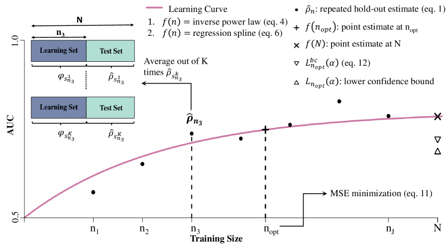
Figure 1: Summary of Learn2Evaluate. First, we estimate the $AUC$ for several training sample sizes $n_{j}$ by repeated hold-out estimation, rendering a learning trajectory (black dots). We smooth this trajectory by an inverse power law or a constrained regression spline, leading to a relationship $f(n)$ between the training set size $n$ and the AUC. We then estimate the predictive performance $\rho_{D}$ by $f(N)$ (black cross). The learning curve also allows us to determine a lower confidence bound (upward triangle) at an optimal training set size $n_{opt}$ (dotted vertical line), which we determine by MSE minimization. To obtain a tighter confidence bound, a bias correction is performed (downward triangle).

2.4.3 Bias-corrected confidence bound

Our predictive performance point estimate for $\rho_{D}$ is $f(N)$ (Figure 1, black cross) and our confidence bound for $\rho_{D}$ equals $L_{n_{opt}}(\alpha)$ (Figure 1, upward triangle), with $n_{opt}$ determined by (11). This confidence bound may be tightened by performing a bias correction. $L_{n_{opt}}$ is in principle a confidence bound for $\rho_{n_{opt}},$ although it is also valid for $\rho_{D}.$ Hence, we may perform an empirical bias correction to $L_{n_{opt}}$ (Figure 1, downward triangle), which leads to

$$L^{bc}_{n_{opt}}(\alpha)=L_{n_{opt}}(\alpha)+\left(f(N)-f(n_{opt})\right).$$ (12)

Correcting for the empirical bias depends on the validity of our point estimate $f(N),$ which we assess in a simulation study.

3 Simulation study

To verify Learn2Evaluate, we evaluate the quality of the point estimate $f(N),$ and the theoretically justified confidence bound $L_{n_{opt}}(\alpha)$ and its bias-corrected version $L^{bc}_{n_{opt}}(\alpha)$ in a high-dimensional simulation study. We focus on classification and the AUC as performance metric.

3.1 Description of experiments

The binary response is generated via

$$Y_{i}\sim\mbox{Bern}\left(\frac{\exp\left(\boldsymbol{X}_{i}\boldsymbol{\beta}\right)}{1+\exp\left(\boldsymbol{X}_{i}\boldsymbol{\beta}\right)}\right)\qquad i=1,\ldots,N,$$ (13)

with covariates $\boldsymbol{X}_{i}\sim\mathcal{N}\left(0_{p},\varSigma_{p\times p}\right),$ where $p=2000$, and elements of the parameter vector $\beta_{1}\ldots\beta_{p}\sim\mbox{Expo}(\nu).$ To mimic a realistic correlation structure between the features, we define $\varSigma_{p\times p}$ as the estimated variance-covariance matrix from a real high-dimensional omics data set described in Best et al. [2015], from which we randomly select $2000$ genes as covariates. This matrix is estimated by a shrinkage method [Schäfer and Strimmer, 2005] implemented in the R package corpcor [Schäfer et al., 2017]. Parameter vector $\boldsymbol{\beta}$ is defined such that a dense covariate-response structure is present, which is often the case in omics applications [Boyle et al., 2017]. We vary the sample size $N$ ($N=100$ and $N=200$) and the signal in the data by tuning rate parameter $\nu$ ($\nu=1000$ and $\nu=100$).

For each setting, specified by $N$ and $\nu$, we simulate $R=1000$ data sets. We then apply Learn2Evaluate to each data set for three learners: ridge regression, lasso regression, both implemented in the R package glmnet [Friedman et al., 2010], and random forest, for which we employ the R package randomforestSRC [Ishwaran and Kogalur, 2021]. We generate learning curves by first estimating the AUC by repeated hold-out estimation ($50$ repeats) for ten subsample sizes $n_{j}$ homogeneously spread over the sample size range $\left[20,N-10\right]$. For ridge and lasso regression, we estimate the penalty parameter for each $n_{j}$ by the median of repeated ($5$ times) $10$-fold CV. This median is fixed for the $50$ repeats of each $n_{j}$. We obtain the learning curve by smoothing the AUC point estimates at different subsample sizes by either the inverse power law or the constrained regression spline. We then estimate the AUC by $f(N)$ and 95% lower confidence bounds by $L_{n_{opt}}(0.05)$ and its bias-corrected version $L^{bc}_{n_{opt}}(0.05).$ We determine $n_{opt}$ by MSE minimization given by (11), using the asymptotic AUC variance estimator (eq. 5 of supplementary Section 2).

We denote $f(N)$ by $f_{r}(N)$ for the $r$th simulated data set, and we approximate the true AUC by $\mbox{AUC}_{r}$: the AUC of the $r$th learned model evaluated on $25,000$ independent test samples. The average $\mbox{AUC}_{r}$ (of $R=1000$ simulation runs) is given in the Appendix (Table A1).

We assess the quality of point estimates $f_{r}(N)$ by the root mean square error (RMSE) and the averaged bias (Bias),

$$\mbox{RMSE}=\sqrt{\frac{1}{R}\sum_{r=1}^{R}\left(f_{r}(N)-\mbox{AUC}_{r}\right)^{2}}\quad\mbox{and}\quad\mbox{Bias}=\frac{1}{R}\sum_{r=1}^{R}\left(f_{r}(N)-\mbox{AUC}_{r}\right).$$ (14)

Confidence bounds $L_{n_{opt}}(0.05)$ and $L^{bc}_{n_{opt}}(0.05)$ are evaluated by their coverage, i.e. the proportion of times the confidence bound is lower than $\mbox{AUC}_{r},$ and the distance of each confidence bound to its corresponding $\mbox{AUC}_{r}.$

We compare Learn2Evaluate, fitted by an inverse power law (L2E-P) or a spline (L2E-S), with two methods that produce a point estimate and a lower confidence bound. Firstly, we consider ten-fold cross-validation (10F-CV). Point estimates are given by the average of the ten test folds and a lower confidence bound is obtained by employing an asymptotic variance estimator, which is derived by LeDell et al. [2015] and implemented in the R package cvAUC [LeDell et al., 2014]. Secondly, we consider leave-one-out bootstrapping (LOOB) [Efron and Tibshirani, 1994] with $500$ bootstrapped training sets and complementary test sets. From the $500$ AUC estimates, we obtain a point estimate and a lower confidence bound by taking the average and the 5% quantile, respectively. Details on the code are found in supplementary Section 9.

3.2 Point estimate evaluation

The RMSE and the averaged bias of the point estimates are given in Table 1.

Table 1: Root mean square error (RMSE) and averaged bias (Bias) of Learn2Evaluate, fitted by an inverse power law (L2E-P) or a constrained regression spline (L2E-S), 10-fold CV (10F-CV), and leave-one-out bootstrapping (LOOB).

		Ridge		Lasso		RF
		RMSE	Bias	RMSE	Bias	RMSE	Bias
	L2E-P	0.053	0.004	0.058	0.009	0.048	0.020
$N=100,$	L2E-S	0.054	0.007	0.070	0.025	0.050	0.026
$\nu=1000$	10F-CV	0.056	-0.001	0.084	-0.009	0.051	0.017
	LOOB	0.071	-0.039	0.057	-0.020	0.050	-0.013
	L2E-P	0.037	0.002	0.048	0.002	0.037	0.002
$N=100,$	L2E-S	0.038	0.004	0.056	0.009	0.038	0.005
$\nu=100$	10F-CV	0.039	0	0.062	-0.005	0.039	0.001
	LOOB	0.048	-0.028	0.051	-0.025	0.043	-0.018
	L2E-P	0.036	0.001	0.041	0.004	0.034	0.002
$N=200,$	L2E-S	0.038	0.004	0.046	0.010	0.034	0.004
$\nu=1000$	10F-CV	0.039	-0.002	0.050	-0.004	0.035	0.009
	LOOB	0.060	-0.041	0.052	-0.034	0.036	-0.009
	L2E-P	0.024	0	0.031	0.001	0.026	0.007
$N=200,$	L2E-S	0.025	0.002	0.035	0.004	0.027	0.008
$\nu=100$	10F-CV	0.025	-0.001	0.036	-0.005	0.026	0.008
	LOOB	0.035	-0.022	0.037	-0.022	0.026	-0.006

The inverse power law (L2E-P) is the overall winner in terms of RMSE, although sometimes, in particular for the random forest (RF), differences are small. In one case (lasso, $N=100,$ $\nu=1000$), leave-one-out bootstrapping (LOOB) has a slightly better RMSE than L2E-P. Table 1 also suggest that the inverse power law (parametric) has a smaller RMSE than the constrained regression spline (nonparametric).

For the averaged bias, the situation is less straightforward. Learn2Evaluate always has a positive bias, whereas the competing methods mostly have a negative bias. The bootstrap often has the most biased estimate. Only for the lasso and the random forest in the $N=100,$ $\nu=1000$ setting and the random forest in the $N=200,$ $\nu=100$ setting is this not the case. L2E-P, which is always (somewhat) less biased than L2E-S, is competitive to 10-fold CV (10F-CV).

A comparison between the learners reveals that the lasso has the largest RMSE for all simulation settings and predictive performance estimators, except for the bootstrap in settings $N=100,$ $\nu=1000$ and $N=200,$ $\nu=1000.$ This finding may be explained by the slope of the learning curve at the end of the learning trajectory. A large slope causes a drop in predictive performance when it is estimated on a subset of the data set, as is the case for 10-fold CV and bootstrapping. Learn2Evaluate also suffers from a larger slope because extrapolation to $N$ becomes more sensitive to errors.

3.3 Confidence bound evaluation

Coverage probabilities for confidence bounds $L_{n_{opt}}(0.05)$ and $L^{bc}_{n_{opt}}(0.05)$ are given in Table 2, with $n_{opt}$ determined by MSE minimization. We also evaluate the asymptotic 10-fold CV confidence bound estimator for the AUC (Le Dell) and leave-one-out bootstrapping (LOOB). We show results for the learning curve fitted by an inverse power law. In supplementary Section 3 (Table S1), we show coverage results when $n_{opt}$ is determined by controlling for the empirical bias instead of MSE minimization. These coverage results are similar as in Table 2. Results for the constrained regression spline are found in supplementary Section 4 (Table S2).

Table 2: Coverage results for the 95% lower confidence bounds of Learn2Evaluate with ($L_{n_{opt}}^{bc}$) and without bias correction ($L_{n_{opt}}$), the asymptotic AUC variance estimator of Le Dell (Le Dell), and leave-one-out bootstrapping (LOOB). The learning curve is fitted by a power law and $n_{opt}$ is determined by MSE minimization.

		Ridge	Lasso	RF			Ridge	Lasso	RF
	$L_{n_{opt}}$	0.976	0.992	0.980		$L_{n_{opt}}$	0.974	0.991	0.975
$\boldsymbol{N=100,}$	$L_{n_{opt}}^{bc}$	0.949	0.935	0.937	$\boldsymbol{N=100,}$	$L_{n_{opt}}^{bc}$	0.941	0.977	0.953
$\boldsymbol{\nu=1000}$	Le Dell	0.895	0.851	0.876	$\boldsymbol{\nu=100}$	Le Dell	0.870	0.847	0.892
	LOOB	0.990	0.996	0.990		LOOB	0.993	0.995	0.995
	$L_{n_{opt}}$	0.992	0.995	0.991		$L_{n_{opt}}$	0.981	0.996	0.969
$\boldsymbol{N=200,}$	$L_{n_{opt}}^{bc}$	0.965	0.969	0.970	$\boldsymbol{N=200,}$	$L_{n_{opt}}^{bc}$	0.960	0.974	0.934
$\boldsymbol{\nu=1000}$	Le Dell	0.911	0.874	0.884	$\boldsymbol{\nu=100}$	Le Dell	0.908	0.886	0.869
	LOOB	0.996	1,00	0.992		LOOB	0.996	0.998	0.989

Table 2 demonstrates that $L_{n_{opt}}(0.05)$ controls the type-I error well below the nominal level, while being less conservative than leave-one-out bootstrapping. Coverage is closer to nominal level for $L^{bc}_{n_{opt}}(0.05)$. In one instance (random forest, $N=200,$ $\nu=100$, $L^{bc}_{n_{opt}}$), the coverage drops just below 95% when taking the binomial error of the coverage estimate into account. When the learning curve is fitted by a constrained regression spline, $L^{bc}_{n_{opt}}(0.05)$ is too liberal in three cases (supplementary Table S2). This result is explained by the worse point estimates of the spline compared to the power law. The asymptotic confidence bound estimator (Le Dell) is too liberal for small sample sizes, similar as in LeDell et al. [2015].

In supplementary Section 5 (Figures S2, S3, S4, and S5), we depict boxplots of the distance of the lower confidence bound to the corresponding target parameter $\mbox{AUC}_{r}$ for the bootstrap, and Learn2Evaluate with ($L^{bc}_{n_{opt}}$) and without ($L_{n_{opt}}$) bias correction. These boxplots show that $L_{n_{opt}}$ and $L^{bc}_{n_{opt}}$ are on average closer to the target parameter $\mbox{AUC}_{r}$ than bootstrapping, with an exception of $L_{n_{opt}}$ for the lasso. The bias correction shortens the distance compared to the confidence bound without bias correction.

The coverage results and the boxplots also illustrate that $L_{n_{opt}}$ for lasso regression is further away from $\mbox{AUC}_{r}$ than for ridge regression and random forest. The average optimal training set size $n_{opt}$ for lasso regression is larger than for ridge regression and random forest (Appendix Table B1). Hence, the average test set size for lasso regression is smaller, which leads to wider confidence bounds. For $L^{bc}_{n_{opt}}$, the difference between the learners is smaller.

4 Applications

4.1 Classification

We apply Learn2Evaluate to messenger-RNA sequencing data, extracted from blood platelets, as described in Best et al. [2015]. These experiments demonstrated that RNA profiles of blood platelets are a promising diagnostic tool for early cancer detection.

RNA profiles of blood platelets from $230$ patients, having one of the in total six tumor types, and $55$ healthy controls were obtained. The raw data are online available in the GEO database (GEO: GSE68086). Data preprocessing is described in Novianti et al. [2017]. Processed data are available via https://github.com/JeroenGoedhart/Learn2Evaluate as well as the R code to apply Learn2Evaluate to these data. For additional details on the data and the code, we refer to supplementary Section 9.

Here, we consider three binary classification cases: non-small-cell lung cancer $(\mbox{NSCLC,}\quad n=60)$ versus the control group $(n=55)$ using $p=19,300$ transcripts (2(a)), breast cancer $(\mbox{Breast,}\quad n=40)$ versus NSCLC using $p=18,741$ transcripts (2(b)), and breast cancer versus pancreas cancer $(\mbox{Pancreas,}\quad n=35)$ using $p=18,350$ transcripts (2(c)). For three other binary classification experiments, we refer to supplementary Section 6 (Figure S6).

Next, we generate learning curves for ridge regression (black), lasso regression (blue), and random forest (green). Learning curves are obtained by the same procedure as in the simulation study. For ten homogeneously spaced subsample sizes, we estimate the predictive performance, quantified by the AUC, by repeated ($50$ times) hold-out estimation. This renders the learning trajectory (dots), i.e. (2). The maximum subsample size equals $N-10.$ We varied the number of different subsamples and repeats to establish that these defaults yield stable estimates (supplementary Section 8, Table S3). We then fit an inverse power law given by (4) (solid line) because this fit obtained the best performance estimates in the simulation.

We construct confidence bounds based on Learn2Evaluate without bias correction ($L_{n_{opt}}$, upward triangle), Learn2Evaluate with bias correction ($L^{bc}_{n_{opt}}$, downward triangle), and leave-one-out bootstrapping (Bootstrap, square). We use MSE minimization, i.e. (11), to determine an optimal training subsample size $n_{opt}$ (dashed vertical line). We also display the point estimates of Learn2Evaluate (star).

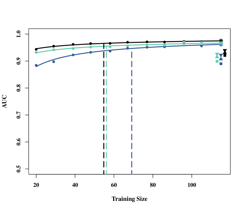
(a) Control vs. NSCLC

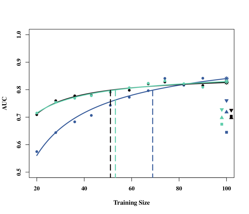
(b) Breast vs. NSCLC

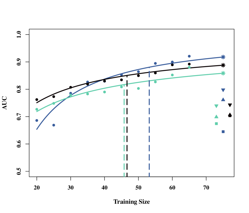
(c) Breast vs. Pancreas

Figure 2: Learning curves for three classification tasks. In each task, we produce a learning curve for a ridge (black), a lasso (blue), and a random forest (green) model. For each learner, we depict the learning trajectory (dots) together with the inverse power law fit (solid line). We show confidence bounds of Learn2Evaluate with ($L^{bc}_{n_{opt}}$, downward triangle) and without ($L_{n_{opt}}$, upward triangle) bias correction, and bootstrapping (Bootstrap, square). We use MSE minimization to determine $n_{opt}$ (dashed vertical line).

Figure 2 and supplementary Figure S6 illustrate that the theoretically justified confidence bound of Learn2Evaluate ($L_{n_{opt}}$) is, in most cases, slightly tighter than the bootstrap confidence bound, which agrees with the simulation results. A bias correction ($L^{bc}_{n_{opt}}$) tightens the theoretically justified bound as expected. Furthermore, Figure 2 shows that $n_{opt}$ adapts to the saturation level of the learning curve. A more saturated curve leads to a smaller training set and hence to a larger test set to determine the lower bound.

Figure 2 and supplementary Figure S6 also illustrate the additional benefits of using learning curves for predictive performance estimation. Firstly, the curves indicate how future samples increase the AUC. For lasso regression, which has in most cases a large slope, additional samples are expected to increase the predictive performance. The ridge and random forest level off completely in 2(a), suggesting that future samples do not increase the AUC.

Secondly, the curves provide a more complete comparison between learners than just employing single point estimates. For example, point estimates of the lasso and the ridge are almost similar in 2(b). The lasso model may still be preferred because its learning curve has a larger slope, which likely leads to a larger increase in the AUC when additional training samples are available.

Finally, the curves show different learning rates. The lasso model tends to be a slow learner. At small subsample sizes, it performs much worse than the ridge and random forest model, but it catches up at larger subsample sizes.

4.2 Regression

The level of methylation of CpG islands has been shown to be predictive of age [Numata et al., 2012]. Here, we apply Learn2Evaluate to a DNA methylation data set ($N=108$ and $p=2289$), which is used to accurately predict age. The predictive performance is quantified by the PMSE. Details on this data set and the learning curves are found in supplementary Section 7 (Figure S7).

Figure S7 illustrates that the decreasing and convex power law fits the learning trajectories for the PMSE well. The upper confidence bounds of Learn2Evaluate are in most cases tighter than the bootstrapped confidence bounds. Only the theoretically justified confidence bound $L_{n_{opt}}$ of random forest is more conservative. The bias-corrected confidence bounds $L^{bc}_{n_{opt}}$ are always tighter than the bootstrapped confidence bounds. Again, the optimal training size $n_{opt}$ adapts to the saturation level of the curves.

Lasso regression has a smaller PMSE than ridge regression and random forest in this application. Interestingly, the bias-corrected confidence bound ($L^{bc}_{n_{opt}}$) of lasso regression is lower valued than the point estimates of ridge regression and random forest, which suggests a clear difference between the learners.

5 Discussion

We presented a novel method, called Learn2Evaluate, to estimate the predictive performance. Learn2Evaluate facilitates the computation of a point estimate and a lower confidence bound, which is proven to control type-I error. This bound may be further tightened by correcting for the estimated bias. This bias-corrected bound is shown to approximately control type-I error in a simulation, although the nominal confidence level is not always guaranteed. Simulations and applications to omics data showed that both bounds are less conservative than a bootstrapped confidence bound. Learn2Evaluate appears to have a lower RMSE of performance point estimates than 10-fold cross-validation and leave-one-out bootstrapping. Furthermore, Learn2Evaluate comes with some additional benefits by providing a dynamic comparison between learners and insight in the potential benefit of future samples.

One practical limitation of Learn2Evaluate is its computational time because of the relatively large number of splits in a training and test set. This may be a drawback in medium to large sample size settings, because computationally more efficient (asymptotic) methods often suffice [LeDell et al., 2015]. However, for small sample sizes, other resampling techniques also need to generate a large number of splits in a training and test set to yield a reliable performance estimator [Jiang and Simon, 2007, Jiang et al., 2008, Kim, 2009].

In the simulations and the applications, we focused on high dimensional data settings with sample sizes ranging from $N=75$ to $N=200$. We focused on omics data by estimating the covariate correlation structure from an omics experiment and by imposing a dense structure on the parameter vector $\boldsymbol{\beta}.$ However, Learn2Evaluate applies to any data setting and covariate-response structure. Evaluating the practical usefulness of Learn2Evaluate for such generalizations requires additional simulations.

Results in this study suggest that the power law, which uses all subsample sizes equally, obtains better point estimates than the regression spline, which predominantly uses training set sizes at the end of the learning trajectory to extrapolate. It is therefore interesting to investigate which subsample sizes are most informative for estimating the performance at the full sample size. This may lead to an optimal weighting scheme in the nonlinear least squares fit by an inverse power law, which may improve our point estimates further. Finding an optimal weighting scheme, however, is nontrivial. The variance of the repeated hold-out estimates is difficult to asses because it depends on the complex correlation structure between overlapping training sets [Bengio and Grandvalet, 2004]. We therefore leave this for future research.

Declaration of Interest

The authors declare no competing interests.

Appendix A Average True AUC

Table A1: Average true AUC for the different simulation settings and learners

	Ridge	Lasso	RF
$N=100,$ $\nu=1000$	0.77	0.71	0.75
$N=100,$ $\nu=100$	0.88	0.83	0.87
$N=200,$ $\nu=1000$	0.78	0.74	0.76
$N=200,$ $\nu=100$	0.89	0.86	0.87

Appendix B Average Training Set Size

Table B1: Average $n_{opt}$ for ridge regression, lasso regression, and random forest (RF).

	Ridge	Lasso	RF
$N=100,$ $\nu=1000$	32	45	33
$N=100,$ $\nu=100$	36	54	34
$N=200,$ $\nu=1000$	69	101	76
$N=200,$ $\nu=100$	76	109	69

Appendix C Supplementary material

Section 1 presents a method to deal with S-shaped learning curves, which may arise as a consequence of a phase transition. Figure S1 shows an instance of a S-shaped learning curve. In Section 2, we show asymptotic variance estimators for the AUC and the PMSE. If such an estimator is not available for the given performance metric, we describe an alternative method in Section 3. Table S1 shows coverage results for this alternative and in Section 4, coverage results for the learning curve fitted by a constrained regression spline are presented. In Section 5, we show boxplots depicting the distance of the confidence bounds of Learn2Evaluate to the true performance (Figures S2, S3, S4, and S5). Section 6 deals with an additional classification application (Figure S6) and in Section 7, Learn2Evaluate is applied in a regression setting. Table S3 (Section 8) shows the stability of the point estimates of Learn2Evaluate with respect to the length of the learning trajectory. Finally, Section 9 gives additional details on the data and the software.

References

- Bamber [1975] D. Bamber. The area above the ordinal dominance graph and the area below the receiver operating characteristic graph. J. Math. Psychol., 12(4):387–415, 1975. doi: 10.1016/0022-2496(75)90001-2.
- Bengio and Grandvalet [2004] Y. Bengio and Y. Grandvalet. No unbiased estimator of the variance of k-fold cross-validation. J. Mach. Learn. Res., 5:1089–1105, 2004. URL https://jmlr.csail.mit.edu/papers/v5/grandvalet04a.html.
- Best et al. [2015] M. G. Best, N. Sol, I. Kooi, J. Tannous, B. A. Westerman, F. Rustenburg, et al. Rna-seq of tumor-educated platelets enables blood-based pan-cancer, multiclass, and molecular pathway cancer diagnostics. Cancer cell, 28(5):666–676, 2015. doi: 10.1016/j.ccell.2015.09.018.
- Boyle et al. [2017] E. A. Boyle, Y. I. Li, and J. K. Pritchard. An expanded view of complex traits: From polygenic to omnigenic. Cell, 169(7):1177–1186, 2017. doi: 10.1016/j.cell.2017.05.038.
- Brier [1950] G. W. Brier. Verification of forecasts expressed in terms of probability. Mon. Weather. Rev., 78(1):1–3, 1950. doi: 10.1175/1520-0493(1950)078¡0001:vofeit¿2.0.co;2.
- Burman [1989] P. Burman. A comparative study of ordinary cross-validation, v-fold cross-validation and the repeated learning-testing methods. Biometrika, 76(3):503–514, 1989. doi: 10.2307/2336116.
- Byrd et al. [1995] R. H. Byrd, P. Lu, J. Nocedal, and C. Zhu. A limited memory algorithm for bound constrained optimization. SIAM J. Sci. Comput., 16(5):1190–1208, 1995. doi: 10.1137/0916069.
- Cortes et al. [1993] C. Cortes, L. D. Jackel, S. Solla, V. Vapnik, and J. Denker. Learning curves: Asymptotic values and rate of convergence. 6:327–334, 1993. URL https://proceedings.neurips.cc/paper/1993/file/1aa48fc4880bb0c9b8a3bf979d3b917e-Paper.pdf.
- DeLong et al. [1988] E. R. DeLong, D. M. DeLong, and D. L. Clarke-Pearson. Comparing the areas under two or more correlated receiver operating characteristic curves: a nonparametric approach. Biometrics, 44(3):837–845, 1988. doi: 10.2307/2531595.
- Dobbin [2009] K. K. Dobbin. A method for constructing a confidence bound for the actual error rate of a prediction rule in high dimensions. Biostatistics, 10(2):282–296, 2009. doi: 10.1093/biostatistics/kxn035.
- Dobbin and Simon [2011] K. K. Dobbin and R. M. Simon. Optimally splitting cases for training and testing high dimensional classifiers. BMC Med. Genomics., 4(1):1–8, 2011. doi: 10.1186/1755-8794-4-31.
- Donoho and Tanner [2005] D. L. Donoho and J. Tanner. Sparse nonnegative solution of underdetermined linear equations by linear programming. P. Natl. Acad. Sci. USA., 102(27):9446–9451, 2005. doi: 10.1073/pnas.0502269102.
- Efron and Tibshirani [1994] B. Efron and R. J. Tibshirani. An introduction to the bootstrap. CRC press, 1994. doi: 10.1201/9780429246593.
- Faber [1999] N. M. Faber. Estimating the uncertainty in estimates of root mean square error of prediction: application to determining the size of an adequate test set in multivariate calibration. Chemometr. Intell. Lab., 49(1):79–89, 1999. doi: 10.1016/s0169-7439(99)00027-1.
- Friedman et al. [2010] J. Friedman, T. Hastie, and R. J. Tibshirani. Regularization paths for generalized linear models via coordinate descent. J. Stat. Softw., 33(1):1–22, 2010. doi: 10.1163/ej.9789004178922.i-328.7.
- Hanley and McNeil [1982] J.A. Hanley and B. J. McNeil. The meaning and use of the area under a receiver operating characteristic (roc) curve. Radiology, 143(1):29–36, 1982. doi: 10.1148/radiology.143.1.7063747.
- Hess and Wei [2010] K. R. Hess and C. Wei. Learning curves in classification with microarray data. Sem. Onc., 37(1):65–68, 2010. doi: 10.1053/j.seminoncol.2009.12.002.
- Ishwaran and Kogalur [2021] H. Ishwaran and U. B. Kogalur. Fast Unified Random Forests for Survival, Regression, and Classification (RF-SRC), 2021. URL https://cran.r-project.org/package=randomForestSRC.
- Jiang and Simon [2007] W. Jiang and R. M. Simon. A comparison of bootstrap methods and an adjusted bootstrap approach for estimating the prediction error in microarray classification. Stat. Med., 26(29):5320–5334, 2007. doi: 10.1002/sim.2968.
- Jiang et al. [2008] W. Jiang, S. Varma, and R. M. Simon. Calculating confidence intervals for prediction error in microarray classification using resampling. Stat. Appl. Genet. Mol., 7(1), 2008. doi: 10.2202/1544-6115.1322.
- Kim [2009] J. H. Kim. Estimating classification error rate: Repeated cross-validation, repeated hold-out and bootstrap. Comput. Stat. Data Anal., 53(11):3735–3745, 2009. doi: 10.1016/j.csda.2009.04.009.
- LeDell et al. [2014] E. LeDell, M. L. Petersen, and M. J. van der Laan. Package cvAUC, 2014. URL https://cran.r-project.org/web/packages/cvAUC/index.html.
- LeDell et al. [2015] E. LeDell, M. L. Petersen, and M. J. van der Laan. Computationally efficient confidence intervals for cross-validated area under the roc curve estimates. Electron. J. Stat., 9 1(1):1583–1607, 2015. doi: 10.1214/15-ejs1035.
- Michiels et al. [2005] S. Michiels, S. Koscielny, and C. Hill. Prediction of cancer outcome with microarrays: a multiple random validation strategy. The Lancet, 365(9458):488–492, 2005. doi: 10.1016/s0140-6736(05)17866-0.
- Mukherjee et al. [2003] S. Mukherjee, P. Tamayo, S. Rogers, R. Rifkin, A. Engle, C. Campbell, et al. Estimating dataset size requirements for classifying dna microarray data. J. Comput. Biol., 10(2):119–142, 2003. doi: 10.1089/106652703321825928.
- Ng and Maechler [2007] P. Ng and M. Maechler. A fast and efficient implementation of qualitatively constrained quantile smoothing splines. Stat. Model., 7(4):315–328, 2007. doi: 10.1177/1471082X0700700403.
- Ng and Maechler [2020] P. Ng and M. Maechler. COBS – Constrained B-splines (Sparse matrix based), 2020. URL https://CRAN.R-project.org/package=cobs.
- Novianti et al. [2017] P. W. Novianti, B. C. Snoek, S. M. Wilting, and M. A Van De Wiel. Better diagnostic signatures from rnaseq data through use of auxiliary co-data. Bioinformatics, 33(10):1572–1574, 2017. doi: 10.1093/bioinformatics/btw837.
- Numata et al. [2012] S. Numata, T. Ye, T. Hyde, X. Guitart, R. Tao, M. Wininger, et al. Dna methylation signatures in development and aging of the human prefrontal cortex. Am. J. Hum. Genet., 90:260–72, 2012. doi: 10.1016/j.ajhg.2011.12.020.
- Robin et al. [2011] X. Robin, N. Turck, A. Hainard, N. Tiberti, F. Lisacek, J. C. Sanchez, and M. Müller. proc: an open-source package for r and s+ to analyze and compare roc curves. BMC Bioinformatics, 12(1):77, 2011. doi: 10.1186/1471-2105-12-77.
- Schäfer and Strimmer [2005] J. Schäfer and K. Strimmer. A shrinkage approach to large-scale covariance matrix estimation and implications for functional genomics. Stat. Appl. Genet. Mol., 4(1), 2005. doi: 10.2202/1544-6115.1175.
- Schäfer et al. [2017] J. Schäfer, R. Opgen-Rhein, V. Zuber, M. Ahdesmaki, A. P. D. Silva, and K. Strimmer. Package corpcor, 2017. URL https://CRAN.R-project.org/package=corpcor.
- Sklar [1959] M Sklar. Fonctions de repartition an dimensions et leurs marges. Publ. inst. statist. univ. Paris, 8:229–231, 1959.
- Stone [1974] M. Stone. Cross-validatory choice and assessment of statistical predictions. J. Roy. Stat. Soc. B. Met., 36(2):111–133, 1974. doi: 10.1111/j.2517-6161.1974.tb00994.x.
- van de Wiel et al. [2009] M. A. van de Wiel, J. Berkhof, and W. N. van Wieringen. Testing the prediction error difference between 2 predictors. Biostatistics, 10(3):550–560, 2009. doi: 10.1093/biostatistics/kxp011.