Quark and gluon GPDs at finite skewness from strings in holographic QCD: evolved and compared with experiment

Abstract

We present a framework for constructing Generalized Parton Distributions (GPDs) using holographic QCD in the large $N_{c}$ limit, with a focus on low-x and finite skewness. Our approach utilizes holographic amplitudes for exclusive electroproduction processes to extract the spin-j conformal (Gegenbauer) moments of GPDs, which are then evolved to higher resolution scales using QCD evolution equations. Our evolved GPDs (reconstructed from their evolved conformal moments) are applied to analyze the electroproduction of $\rho^{0,+}$ and $\phi$ mesons, and we account for non-perturbative contributions in the $s+u$ - channel using holographic QCD. The results compare well with the existing experimental data. Our GPDs provide detailed information about partonic distributions and are useful for future experimental studies and global data analyses.

I Introduction

The General Parton Distributions (GPDs) provide a comprehensive framework for addressing the longitudinal momentum and spatial distributions of partons in hadrons. They consolidate the physical content of form factors, parton distribution amplitudes (DA), and parton distribution functions (PDFs) into a single framework. A number of current and future electron machines, such as the EIC and EIcC Abdul Khalek et al. (2021); Anderle et al. (2021), will be dedicated to measuring them.

The GPDs capture several invariants of the off-forward and non-local quark or gluon bilinears. In this work, we will focus on the unpolarized quark and gluon GPDs $H(x,\eta,t)$ and quark axial GPDs $\widetilde{H}(x,\eta,t)$ in the large $N_{c}$ limit. For the quarks, they can be combined into valence (isovector) and singlet GPDs. GPDs are a function of the parton longitudinal momentum fraction $x$, the skewness $\eta\sim\xi=-\Delta^{+}/2P^{+}$, and the momentum transfer $\Delta^{2}=-t$. $\Delta^{+}$ and $P^{+}$ are the light front momentum transfer and averaged momentum of the in-out protons, respectively.

The GPDs are characterized by two distinct kinematical regions for fixed Mandelstam $t$ and positive skewness: the DGLAP regions for $|x|>\xi$ and the ERBL region for $|x|<\xi$. In the DGLAP region with positive (negative) $x$, the GPDs correspond to removing a quark (antiquark) with momentum $k$ and re-inserting it with momentum $k+\Delta$. In the ERBL region, the GPDs correspond to emitting a meson-like quark-antiquark pair with momentum $-\Delta$. As a result, the forward limit with zero skewness of the GPDs coincides with the quark and gluon PDFs, while the x-integrated GPDs with finite skewness coincide with form factors.

GPDs play an important role in exclusive processes and are at the cornerstone of hadronic tomography. Deeply Virtual Compton Scattering (DVCS) is one of the processes suggested for the empirical extraction of the GPDs Ji (1997); Radyushkin (1997). Assuming factorization, the invariant Compton amplitudes are usually expressed as integral transforms of the leading twist-2 quark operators in the form of generalized sum rules. The extraction of the quark GPDs requires their inversion, usually using a perturbative analysis of the pertinent moments. This is a non-trivial deconvolution problem Bertone et al. (2021).

Holographic QCD provides a non-perturbative approach to a variety of scattering processes in QCD in the double limit of a large number of colors and strong ^′t Hooft gauge coupling. It is a proposal following on the AdS/CFT or gauge/gravity duality established in string theory Nastase (2015). In short, a strongly coupled gauge theory in four dimensions is dual to weakly coupled string theory in higher dimensions. The original correspondence holds for type IIB superstring theory in $AdS_{5}\times S_{5}$, but is commonly assumed to hold for a string theory in a general background.

In this work, we propose to use holographic QCD with a soft wall to evaluate electroproduction of photons and mesons by combining the leading s- and t-channel exchanges at finite skewness. The t-channel exchanges are dominated by open and closed string exchanges in the double limit, and they are dominant in the Regge kinematics.

A key outcome from this construction is exclusive amplitudes with a well-defined dependence on all kinematical variables. This yields well-defined expressions for the initial quark and gluon GPDs in the ERBL region to evolve at higher resolution with the help of perturbative renormalization group equations. The interface between the perturbative and non-perturbative and stringy aspects of QCD will be shown to set in for a gauge coupling $\alpha_{s}(\mu_{0})\sim\frac{1}{3}$ at a resolution $\mu_{0}\sim 1.8$ GeV.

In our analysis, the deconvolution problem is altogether bypassed through the use of Gegenbauer moments for pertinent GPDs. The holographic construction allows their identification for any value of the conformal spin-j in the large number of colors limit. Their spin-j resummation in the GPDs can be carried explicitly in the ERBL region in the Regge limit. The extension to the DGLAP region can be sought using a re-organized Gegenbauer expansion. Once evolved, the results can be used in any exclusive process. They also should prove useful for the extraction of the GPDs in global data analyses. For completeness, we note the holographic GPDs analysis in Nishio and Watari (2014a).

To our knowledge, the holographic framework provides the most economical way to encode the stringy properties of QCD at low resolution, in line with the dual Veneziano amplitudes and empirical Regge phenomenology. In the double limit of large $N_{c}$ and strong ^′t Hooft coupling, the holographic amplitudes capture the key aspects used in QCD dispersive analyses, such as crossing symmetry, unitarity, and spectral densities, all while enforcing the essential symmetries of QCD with very few stringy parameters.

The paper is structured as follows: In section II, we use large $N_{c}$ arguments to extract the conformal moments of GPDs from the holographic exclusive amplitudes for electroproduction of mesons at low-x and low resolution $\mu_{0}$ by matching the holographic exclusive amplitudes with the exclusive amplitudes in QCD which are based on factorization theorems. This matching is done explicitly for the electroproduction of mesons, photons (DVCS), a pair of pions, and a neutral pion. In section III, the extracted conformal moments of GPDs will be evoloved, to higher resolution $\mu$, using Renormalization Group Equations (RGEs). The evolved GPDs will also be reconstructed using their evolved conformal moments. In section IV, we use the evolved singlet quark and gluon GPDs to analyze in detail the electroproduction of neutral $\rho^{0}$. The total and differential cross-sections are derived and compared to the available data for a wide range of energies $\sqrt{s}$ and momentum transfer. In section V, we extend the analysis to the electroproduction of $\phi$, using the evolved gluon GPDs. The results are compared to some existing data. In section VI, we make use of the evolved non-singlet (valence) quark GPDs to derive the total and differential cross-sections for the electroproduction of charged $\rho^{+}$. The results are also compared to existing data, mostly at low $\sqrt{s}$. Our conclusions are in Section VII.

II Conformal moments of GPDs from t-channel string exchange in AdS/QCD

In this paper, we investigate the use of General Parton Distributions (GPDs) in exclusive processes, such as leptoproduction of photons and hadrons, where factorization is assumed to work. GPDs capture the off-forward partonic content of a hadron, and their importance lies in their ability to combine the physical content of form factors, parton distribution amplitudes (DA), and parton distribution functions (PDFs) in a single framework. We focus on the unpolarized quark and gluon GPDs $H(x,\eta,t)$, and quark axial GPDs $\widetilde{H}(x,\eta,t)$, in the large $N_{c}$ limit.

We propose a method to determine the matrix elements that define GPDs at some initial soft renormalization scale $\mu=\mu_{0}$, which carries information on confinement and chiral symmetry breaking, and then evolve them using the Renormalization Group Equation (RGE) to higher $\mu$. Our proposed method involves using holographic QCD, a dual string approach in AdS, in the double limit of large $N_{c}$ and strong ’t Hooft coupling. We identify the twist-2 quark and gluon GPD conformal moments at finite skewness $\eta\neq 0$ and an initial renormalization scale $\mu_{0}\sim Q_{0}$ using various exclusive t-channel open and closed string exchange electroproduction amplitudes in soft-wall holographic QCD, as detailed in Appendix H. The closed strings in soft-wall AdS are dual to spin-j glueballs in QCD, while the open strings attached to bulk filling $N_{f}$ D9-branes in soft-wall AdS are dual to spin-j vector and axial mesons.

We match various exclusive electroproduction amplitudes in holographic QCD to various electroproduction amplitudes in QCD, written in terms of quark and gluon GPDs based on the leading-order factorization theorems, by matching their respective large-$N_{c}$ dependence at fixed ’t Hooft coupling $\lambda_{s}=g_{s}^{2}N_{c}$. We determine the large-$N_{c}$ dependence of the exclusive processes in the holographic side by using the bulk gravitational constant $2\kappa^{2}\sim{1}/{N_{c}^{2}}$ and the bulk D9-brane coupling constant $g_{5}^{2}\sim{1}/{N_{c}}$. The matching of exclusive electroproduction amplitudes is illustrated in Figs. 1 - 4.

We consider only tree-level Witten diagrams in AdS and the leading-order exclusive electroproduction amplitudes in QCD, as they are the only diagrams that contribute in the large-$N_{c}$ limit. The rules for the tree-level Witten diagrams stem from the SUGRA fields and their couplings in bulk, which are detailed in Appendix H. These rules enable us to evaluate electroproduction of photons and mesons in holographic QCD, combining the leading s- and t-channel exchanges at finite skewness, and resulting in exclusive amplitudes with well-defined dependence on all kinematical variables.

In summary, this section presents the proposed method for determining GPDs using holographic QCD in the large $N_{c}$ limit, and summarizes the key results of this paper. The relevant notations and kinematics are summarized in Appendix A, and Appendix B, respectively. The matrix elements that define GPD are detailed in the Appendix C. The RGE used to evolve the matrix elements to higher $\mu$ is detailed in Appendix D. Furthermore, the exclusive electroproduction amplitudes in QCD are summarized in Appendix E, which should be compared with the corresponding holographic amplitudes derived in Appendix H where we have illustrated the comparisons in Figs. 1 - 4.

II.1 Electroproduction of vector mesons

The leading order electroproduction amplitude for vector mesons (with quark DA and gluon GPD) is of order $\frac{g_{s}^{2}}{N_{c}}$ as illustrated in Fig. 1 left. In the large-$N_{c}$ limit, it is of order $\frac{g_{s}^{2}N_{c}}{N_{c}^{2}}=\frac{\lambda_{s}}{N_{c}^{2}}\,.$ This matches the $\frac{1}{N_{c}^{2}}$ dependence for the holographic vector meson electroproduction amplitude, using the corresponding tree-level Witten diagram illustrated in Fig. 1 right. More specifically, the $N_{c}$ dependence of the electroproduction of vector mesons written in terms of Gegenbauer moments,

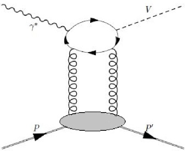
(a)

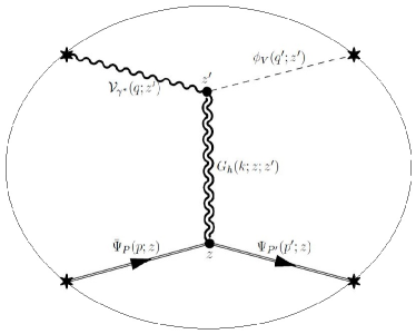
(b)

Figure 1: electroproduction of a vector meson probing the $\mathbf{gluon~{}GPD}$: (a) leading QCD contribution in the Regge limit; (b) leading Witten diagram in the large-$N_{c}$ limit.

$${\cal A}^{LL}_{\gamma^{*}p\rightarrow Vp}(s,t,Q_{0},\epsilon_{L},\epsilon^{\prime}_{L}) \approx e\times\frac{1}{4}\times\frac{1}{N_{c}^{2}}\times\frac{1}{Q_{0}}\times\lambda_{s}(\mu^{2})\times\left[\int_{0}^{1}dz\,\sum_{q}e_{q}\frac{\Phi^{q}(z)}{z(1-z)}\right]\times\frac{1}{m_{N}}\times\bar{u}(p_{2})u(p_{1})$$

$$\times \sum_{j=2}^{\infty}\frac{1}{\xi^{j}}\times\frac{1}{N_{j-2}(\frac{5}{2})}\times\left[\int_{0}^{\xi}\frac{dx}{\xi}\,\left(1-\frac{x^{2}}{\xi^{2}}\right)\times C_{j-2}^{5/2}\left(\frac{x}{\xi}\right)\right]\times\mathbb{F}^{g}_{j}(\xi,t;\mu_{0}^{2})\,,$$

for even $j=2,4,...$, matches the holographic result

$${\cal A}^{LL}_{\gamma^{*}p\rightarrow Vp}(s,t,Q_{0},\epsilon_{L},\epsilon^{\prime}_{L}) \sim e\times\frac{1}{g_{5}}\times g_{5}\times 2\kappa^{2}\times\frac{1}{2}\times\frac{1}{Q_{0}}\times\left[f_{V}\right]\times\frac{1}{m_{N}}\times\bar{u}(p_{2})u(p_{1})$$

$$\times \sum_{j=2}^{\infty}\,\frac{1}{\xi^{j}}\times\left[\frac{1}{\Gamma(\Delta_{g}(j)-2)}\times\left[\mathcal{A}(j,\tau,\Delta_{g}(j),t)+\mathcal{D}_{\eta}(j,\tau,\Delta_{g}(j),t)\right]\right]\,,$$

for even $j=2,4,...$, with the details of the derivation given in Appendix H. The 5-dimensional bulk gravitational coupling is $2\kappa^{2}={8\pi^{2}}/{N_{c}^{2}}$, and $g_{5}\sim 1/\sqrt{N_{c}}$.

A comparison of (II.1) and (II.1), allows the extraction of the Gegenbauer (conformal) moments of the gluon GPDs

$$\mathbb{F}^{g}_{j}(\eta\sim\xi,t;\mu_{0}^{2})\propto\frac{1}{\Gamma(\Delta_{g}(j)-2)}\times\left[\mathcal{A}(j,\tau,\Delta_{g}(j),t)+\mathcal{D}_{\eta}(j,\tau,\Delta_{g}(j),t)\right]\,,$$

with $\eta\sim\xi$ following from $\sqrt{s}\gg-t$, with the details of the kinematics in Appendix B. The anomalous dimension of the spin-j conformal gluon operator at $\mu=\mu_{0}\sim Q_{0}$, and even $j=2,4,...$ is

$$\Delta_{g}(j)=2+\sqrt{2\sqrt{\lambda}(j-j_{0g})}\,,$$

with $j_{0g}=2-2/\sqrt{\lambda}$, and the ’t Hooft coupling of QCD at $\mu=\mu_{0}$ given by

$$\lambda\equiv\lambda_{s}(\mu_{0})=4\pi\alpha_{s}(\mu_{0})N_{c}\rightarrow 11.243\,.$$

Below we suggest the matching scale $\mu_{0}=1.808$ GeV (see section D.4). In addition, we have set the Mandelstam variable $t=-K^{2}$, and defined the $\eta$-independent gluonic spin-j (with even $j=2,4,...$) form factors of the proton (with twist $\tau$) as

$$\mathcal{A}(j,\tau,\Delta_{g}(j),-t=K^{2})=$$

$$\frac{2^{1-\Delta_{g}(j)}}{\Gamma(\tau)}\Bigg{(}(\tau-1)\Gamma\left(\frac{j-2}{2}+\tau-\frac{\Delta_{g}(j)}{2}+1\right)\Gamma\left(\frac{j-2}{2}+\frac{\Delta_{g}(j)}{2}+\tau-1\right)$$

$$\times \,{}_{2}\tilde{F}_{1}\left(\frac{a_{K}}{2}-\frac{\Delta_{g}(j)}{2}+2,\frac{j-2}{2}+\tau-\frac{\Delta_{g}(j)}{2}+1;\frac{a_{K}}{2}+\frac{j-2}{2}+\tau+1;-1\right)$$

$$+\Gamma\left(\frac{j-2}{2}+\tau-\frac{\Delta_{g}(j)}{2}+2\right)\Gamma\left(\frac{j-2}{2}+\frac{\Delta_{g}(j)}{2}+\tau\right)$$

$$\times {}_{2}\tilde{F}_{1}\left(\frac{a_{K}}{2}-\frac{\Delta_{g}(j)}{2}+2,\frac{j-2}{2}+\tau-\frac{\Delta_{g}(j)}{2}+2;\frac{a_{K}}{2}+\frac{j-2}{2}+\tau+2;-1\right)\Bigg{)}\,,$$

where ${}_{2}\tilde{F}_{1}$ is the regularized hypergeometric function, with $a_{K}=K^{2}/4\tilde{\kappa}_{T}^{2}$. The skewness or $\eta$-dependent spin-j $\mathcal{D}_{\eta}$-terms are given by

$$\mathcal{D}_{\eta}(j,\tau,\Delta_{g}(j),-t=K^{2}) = \left(\hat{d}_{j}(\eta,-K^{2})-1\right)\times\left[\mathcal{A}(j,\tau,\Delta_{g}(j),K,\tilde{\kappa}_{T})-\mathcal{A}_{S}(j,\tau,\Delta_{g}(j),K,\tilde{\kappa}_{S})\right]\,,$$

where

$$\mathcal{A}_{S}(j,\tau,\Delta_{g}(j),K,\tilde{\kappa}_{S}) \equiv \mathcal{A}(j,\tau,\Delta_{g}(j),K,\tilde{\kappa}_{T}\rightarrow\tilde{\kappa}_{S})\,.$$ (II.6)

and

$$\hat{d}_{j}(\eta,-K^{2})=\,_{2}F_{1}\left(-\frac{j}{2},\frac{1-j}{2};\frac{1}{2}-j;\frac{4m_{N}^{2}}{K^{2}}\times\eta^{2}\right)\,.$$ (II.7)

Note that the A-form factor for the spin-2 exchange is given by

$$A(t)=\mathcal{A}(j=2,\tau,\Delta_{g}(j=2)=4,-t=K^{2})\,,$$

and the D-form factor for the same spin-2 exchange (the spin-2 D-term) is given by

$$\eta^{2}D(t)=\mathcal{D}_{\eta}(j=2,\tau,\Delta_{g}(j=2)=4,-t=K^{2})\,.$$

Both form factors play an important role in the holographic electroproduction of heavy mesons near treshold Mamo and Zahed (2020, 2021a, 2022) (and references therein).

II.2 Electroproduction of pion pair

The electroproduction amplitude for pair of mesons (with gluon DA and quark GPDs) at leading-order is order of $\frac{g_{s}^{2}}{N_{c}}$. Therefore, in the large-$N_{c}$ limit, it is of order $\frac{g_{s}^{2}N_{c}}{N_{c}^{2}}=\frac{\lambda_{s}}{N_{c}^{2}}\,,$ (see Fig. 2 left). We find the same $\frac{1}{N_{c}^{2}}$ dependence for the holographic meson pair electroproduction amplitude, using the corresponding tree-level Witten diagram (see Fig. 2 right), and compare the $N_{c}$ dependence of the electroproduction of pair mesons written in terms of Gegenbauer momnents (II.2), and the holographic one (II.2) below

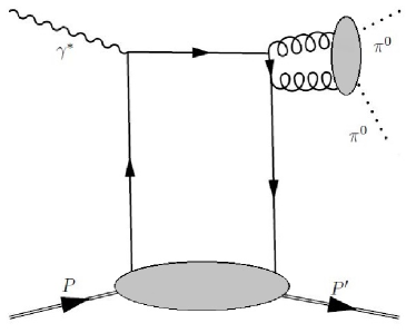
(a)

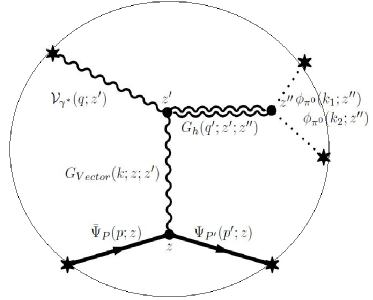
(b)

Figure 2: electroproduction of double pions probing the $\bf{non-singlet~{}(valence)~{}vector~{}quark~{}GPDs}$ : (a) leading QCD contribution in the Regge limit; (b) leading Witten diagram in the large-$N_{c}$ limit.

$${\cal A}^{LL}_{\gamma^{*}p\rightarrow\pi\pi p}(s,t,Q_{0},\epsilon_{L};m_{\pi\pi}) \approx e\times\lambda_{s}(\mu_{0})\times\frac{4}{N_{c}^{2}}\times\frac{1}{Q_{0}}\times\left[\int_{0}^{1}dz\,\frac{\Phi^{g}(z)}{z(1-z)}\right]\times\frac{1}{2m_{N}}\times\bar{u}(p_{2})u(p_{1})$$

$$\times \sum_{j=1}^{\infty}\frac{1}{\xi^{j}}\times\frac{1}{N_{j-1}(\frac{3}{2})}\times\left[\int_{0}^{\xi}\frac{dx}{\xi}\,C_{j-1}^{3/2}\left(\frac{x}{\xi}\right)\right]\times\sum_{q}Q_{q}\,\mathbb{F}^{q}_{j(valence)}(\eta\sim\xi,t;\mu_{0}^{2})\,,$$

for odd $j=1,3,..$, and

$${\cal A}^{LL}_{\gamma^{*}p\rightarrow\pi\pi p}(s,t,Q_{0},\epsilon_{L};m_{\pi\pi}) \sim e\times\frac{1}{g_{5}}\times g_{5}\times 2\kappa^{2}\times\frac{1}{4}\times\frac{1}{Q_{0}}\times\left[A_{gluon}^{\pi}(m_{\pi\pi})\right]\times\frac{1}{2m_{N}}\times\bar{u}(p_{2})u(p_{1})$$

$$\times \sum_{j=1}^{\infty}\,\frac{1}{\xi^{j}}\times\frac{1}{\Gamma(\Delta_{q}(j)-2)}\times\left[\mathcal{F}_{1}(j,\tau,\Delta_{q}(j),t)+\mathcal{D}_{q\eta}(j,\tau,\Delta_{q}(j),t)\right]\,,$$

for odd $j=1,3,....$, with the 5-dimensional bulk gravitational coupling $2\kappa^{2}={8\pi^{2}}/{N_{c}^{2}}$, and $g_{5}\sim 1/\sqrt{N_{c}}$. The detailed derivation of (II.2) is given in Appendix H. Comparing (II.2) to (II.2), we identify the conformal moments

$$\mathbb{F}^{q}_{j(valence)}(\eta\sim\xi,t;\mu_{0}^{2}) \propto \frac{1}{\Gamma(\Delta_{q}(j)-2)}\times\left[\mathcal{F}_{1}(j,\tau,\Delta_{q}(j),t)+\mathcal{D}_{q\eta}(j,\tau,\Delta_{q}(j),t)\right]\,.$$ (II.10)

The anomalous dimension of the spin-j conformal valence quark operator at $\mu=\mu_{0}\sim Q_{0}$, and odd $j=1,3,...$ is given by

$$\Delta_{q}(j)=2+\sqrt{\sqrt{\lambda}(j-j_{0q})}\,,$$

with $j_{0q}=1-1/\sqrt{\lambda}$, and the ’t Hooft coupling at $\mu=\mu_{0}$ fixed as

$$\lambda\equiv\lambda_{s}(\mu_{0})=4\pi\alpha_{s}(\mu_{0})N_{c}=11.243\,.$$

The $t$-dependent valence quark spin-j (with odd $j=1,3,5,7,...$) form factors of the proton with twist $\tau=d-s$, is

$$\mathcal{F}_{1}(j,\tau,\Delta_{q}(j),-t=K^{2}) \propto \mathcal{A}(j\rightarrow j+1,\tau,\Delta_{g}\rightarrow\Delta_{q},t)$$

and the quark spin-j skewness dependent $\mathcal{D}_{q\eta}$-terms are

$$\mathcal{D}_{q\eta}(j,\tau,\Delta_{q}(j),t) \propto \mathcal{D}_{\eta}(j\rightarrow j+1,\tau,\Delta_{g}\rightarrow\Delta_{q},t;\tilde{\kappa}_{T}\rightarrow\frac{1}{2}\times\tilde{\kappa}_{V})\,,$$ (II.12)

where $\mathcal{A}$ and $\mathcal{D}_{\eta}$ are given by (II.1) and (II.1), respectively, for odd $j=1,3,5,7,...$.

Note that the Dirac electromagnetic form factor (ignoring the Pauli contribution) for the spin-1 exchange is given by

$$F_{1}(t)=\mathcal{F}_{1}(j=1,\tau,\Delta_{q}(j=1)=3,-t=K^{2})\,.$$

II.3 DVCS amplitude

The DVCS amplitude in QCD at leading-order is order of $N_{c}^{0}$ (see Fig. 3 left), the NLO correction (due to the gluon GPD contribution) is order of $g_{s}^{2}=\frac{g_{s}^{2}N_{c}}{N_{c}}=\frac{\lambda_{s}}{N_{c}}\,$, and can be ignored in the large-$N_{c}$ and small ’t Hooft coupling limit. Using the corresponding tree-level Witten diagrams (see Fig. 3 right), we find the same $N_{c}^{0}$ dependence for the holographic DVCS amplitudes in the large-$N_{c}$ limit (compare the $N_{c}$ dependence of the axial part of DVCS written in terms of Gegenbauer moments (II.3) and the holographic DVCS (II.3) below,

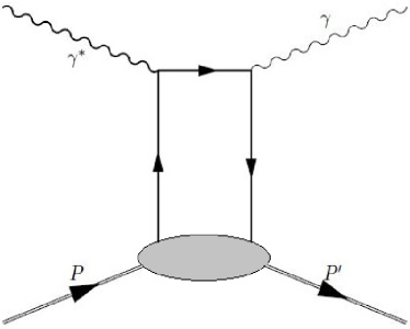
(a)

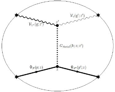
(b)

Figure 3: Deeply virtual Compton scattering (DVCS) probing the $\bf{singlet~{}axial~{}quark~{}GPDs}$ : (a) leading QCD contribution in the Regge limit; (b) leading Witten diagram in the large-$N_{c}$ limit.

$${\cal A}^{LT}_{\gamma^{*}p\rightarrow\gamma p}(s,t,Q_{0},\epsilon_{L},\epsilon^{\prime}_{T}) \approx \!\!\!\epsilon_{L\mu}\epsilon_{T\nu}^{\prime*}\times N_{c}^{0}\times i\varepsilon^{\mu\nu\rho\sigma}\tilde{q}_{\sigma}p_{\rho}\times\frac{1}{p^{+}}\times\bar{u}(p_{2})\gamma^{+}\gamma_{5}u(p_{1})$$

$$\times \frac{4}{Q_{0}^{2}}\times\sum_{j=1}^{\infty}\,\frac{1}{\xi^{j-1}}\times\frac{1}{N_{j-1}(\frac{3}{2})}\times\left[\int_{0}^{\xi}\frac{dx}{\xi}\,C_{j-1}^{3/2}\left(\frac{x}{\xi}\right)\right]\times\sum_{q}Q_{q}^{2}\,\tilde{\mathbb{F}}^{q}_{j(singlet)}(\eta\sim\xi,t;\mu_{0}^{2})\,,$$

for odd $j=1,3,...$, and

$${\cal A}^{LT}_{\gamma^{*}p\rightarrow\gamma p}(s,t,Q_{0},\epsilon_{L},\epsilon^{\prime}_{T}) = \frac{1}{g_{5}}\times\frac{1}{g_{5}}\times g_{5}\times g_{5}^{3}\kappa_{cs}\times\frac{1}{\tilde{\kappa}_{N}^{2}}\epsilon_{L\mu}\epsilon_{T\nu}^{\prime*}\times i\varepsilon^{\mu\nu\rho\sigma}\tilde{q}_{\sigma}\times\bar{u}(p_{2})\gamma_{\rho}\gamma_{5}u(p_{1})$$

$$\times \sum_{j=1}^{\infty}\,\frac{1}{\xi^{j-1}}\times\frac{1}{\Gamma(\Delta_{q}(j)-2)}\times\left[\mathcal{F}_{A}(j,\tau,\Delta_{q}(j),t)+\mathcal{D}_{A\eta}(j,\tau,\Delta_{q}(j),t)\right]\,,$$

for odd $j=1,3,...$ with $g_{5}\sim 1/\sqrt{N_{c}}$ and the Chern-Simons coupling $\kappa_{cs}\sim N_{c}$. The detailed derivation of (II.3) is given in Appendix H. The matching of (II.3) to (II.3) in leading order in $1/N_{c}$, yields

$$\tilde{\mathbb{F}}^{q}_{j(singlet)}(\eta\sim\xi,t;\mu_{0}^{2}) \propto \frac{1}{\Gamma(\Delta_{q}(j)-2)}\times\left[\mathcal{F}_{A}(j,\tau,\Delta_{q}(j),t)+\mathcal{D}_{A\eta}(j,\tau,\Delta_{q}(j),t)\right]\,,$$

where the spin-j axial form factors $\mathcal{F}_{A}(j,\tau,\Delta_{q}(j),t)$ and $\mathcal{D}_{A\eta}(j,\tau,\Delta_{q}(j),t)$ are given by (H.9) and (H.9), respectively, for odd $j=1,3,...$. The anomalous dimension of the spin-j conformal singlet axial quark operator at $\mu=\mu_{0}\sim Q_{0}$, and odd $j=1,3,...$ is given by

$$\Delta_{q}(j)=2+\sqrt{\sqrt{\lambda}(j-j_{0q})}\,,$$

with $j_{0q}=1-1/\sqrt{\lambda}$.

Note that the axial electromagnetic form factor for the spin-1 exchange is given by

$$F_{A}(t)=\mathcal{F}_{A}(j=1,\tau=3,\Delta_{q}(j=1)=3,-t=K^{2})\,.$$

II.4 Electroproduction of neutral pion

Finally, the electroproduction amplitude for mesons (with quark DAs and quark GPDs) at leading-order is order of $\frac{C_{F}g_{s}^{2}}{N_{c}}$ with $C_{F}=\frac{N_{c}^{2}-1}{2N_{c}}$ (see Fig. 4 left). Therefore, the electroproduction amplitude for mesons (with quark DAs and quark GPDs) at leading-order is of order $\frac{g_{s}^{2}N_{c}}{2N_{c}}=\frac{\lambda_{s}}{2N_{c}}\,,$ using $C_{F}\sim\frac{N_{c}}{2}$ in the large-$N_{c}$ limit. We find the same $\frac{1}{N_{c}}$ dependence for the holographic meson electroproduction amplitude using the corresponding tree-level Witten diagram (see Fig. 4 right), and compare the $N_{c}$ dependence of the electroproduction of $\pi^{0}$ written in terms of Gegenbauer momnents (II.4) and the holographic one (II.17) below,

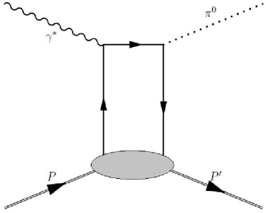
(a)

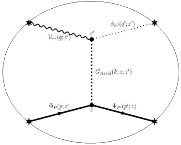
(b)

Figure 4: electroproduction of neutral pion probing the $\bf{non-singlet~{}(valence)~{}axial~{}quark~{}GPDs}$ : (a) leading QCD contribution in the Regge limit; (b) leading Witten diagram in the large-$N_{c}$ limit.

$${\cal A}^{LL}_{\gamma^{*}p\rightarrow\pi^{0}p}(s,t,Q_{0},\epsilon_{L},\epsilon_{L}^{\prime}) \,\approx\, e\times{1\over 2}\times\frac{1}{N_{c}}\times\lambda_{s}(\mu_{0})\times{1\over{Q_{0}}}\times\left[\,\int_{0}^{1}dz{{\Phi_{\pi}(z)}\over z}\right]\times\frac{1}{p^{+}}\times u(p_{2})\gamma^{+}\,\gamma_{5}u(p_{1})\times{-1\over{\sqrt{2}}}$$

$$\times \sum_{j=2}^{\infty}\frac{1}{\xi^{j}}\times\frac{1}{N_{j-1}(\frac{3}{2})}\times\left[\int_{0}^{\xi}\frac{dx}{\xi}\,\frac{x}{\xi}\,C_{j-1}^{3/2}\left(\frac{x}{\xi}\right)\right]$$

$$\times \left(Q_{u}\ \widetilde{\mathbb{F}}^{u}_{j(valence)}(\eta\sim\xi,t;\mu_{0}^{2})\,-\,Q_{d}\ \widetilde{\mathbb{F}}^{d}_{j(valence)}(\eta\sim\xi,t;\mu_{0}^{2})\right)\,,$$

for even $j=2,4,...$, and

$${\cal A}^{LL}_{\gamma^{*}p\rightarrow\pi^{0}p}(s,t,Q_{0},\epsilon_{L},\epsilon_{L}^{\prime}) = e\times\frac{1}{g_{5}}\times g_{5}^{2}\times g_{5}\times\left[f_{\pi}\right]\times\frac{1}{2}\times\frac{1}{Q_{0}}\times\frac{1}{p^{+}}\times\bar{u}(p_{2})\gamma^{+}\,\gamma_{5}u(p_{1})\times\frac{-1}{\sqrt{2}}$$ (II.17)

$$\times\sum_{j=2}^{\infty}\,\frac{1}{\xi^{j}}\times\frac{1}{\Gamma(\Delta_{q}(j)-2)}$$

$$\times \mathcal{F}_{A}(j,\tau,\Delta_{q}(j),t)\times\mathcal{O}\left(1/N_{c}\right)\rightarrow 0\,,$$

for even $j=2,4,...$, with $g_{5}\sim 1/\sqrt{N_{c}}$. The details of the derivation of (II.17) can be found in Appendix H. Note that the holographic amplitude (II.17) is $1/N_{c}$ suppressed since there is no direct coupling between axial-axial-vector mesons at tree level. Similarly, comparing (II.4) to (II.17), the Gegenbauer (conformal) moments of the valence axial GPDs at $\mu=\mu_{0}$ vanish

$$\widetilde{\mathbb{F}}^{q}_{j(valence)}(\eta\sim\xi,t;\mu_{0}^{2}) = 0\,.$$

III RG Evolution of Quark and Gluon GPDs in QCD

In the inclusive DIS process, the hadron’s partonic content varies with the probing virtual photon’s $Q^{2}$. In massless QCD, a scale-free theory, this leads to scaling violations or logarithmic deviations from free partons. DIS structure functions are convolutions of perturbatively determined coefficient functions with fixed $Q^{2}/\mu^{2}$ and relevant PDFs at resolution $\mu$, due to factorization. The PDFs’ evolution and mixing are determined by DGLAP, reflecting the RG flow independence of the original structure functions.

Contrasting with PDFs (diagonal matrix elements of gauge invariant bilocals), GPDs are off-diagonal (double parton distributions) and follow the exclusive kernels’ evolution described by ERBL. The ERBL evolution can be recast into a DGLAP evolution when expressed in terms of hadronic DA moments. Similarly, GPDs’ evolution can be transformed into a DGLAP-type evolution when expressed in terms of Gegenbauer (conformal) moments, as detailed in Belitsky and Radyushkin (2005).

We provide a concise summary of the central RG evolution results for conformal (Gegenbauer) moments derived from the holographic construction at the initial resolution $\mu_{0}$. See Appendix D for detailed derivations. The evolved GPDs, reconstructed from the evolved conformal moments, will be utilized in the electroproduction analysis of $\rho^{0}$, $\phi$, and $\rho^{+}$ vector mesons, and compared with experimental data in sections IV, V, and VI, respectively.

III.1 RG evolution of non-singlet (valence) quark GPDs

The leading-order RG evolution of Gegenbauer (conformal) moments of valence (non-singlet) vector quark GPDs is given by (see Eq.4.244 in Belitsky and Radyushkin (2005))

$$\mathbb{F}^{q}_{j(valence)}(\eta,t;\mu^{2})=\mathbb{F}^{q}_{j(valence)}(\eta,t;\mu_{0}^{2})\times\left(\frac{\alpha_{s}(\mu_{0}^{2})}{\alpha_{s}(\mu^{2})}\right)^{\gamma_{(0)j-1}^{qq;\text{V};\text{NS}}/\beta_{0}}$$ (III.19)

for odd $j=1,3,...$, where the input valence quark GPDs $\mathbb{F}^{q}_{j(valence)}(\eta,t;\mu_{0}^{2})$ are given in (II.10). Hence, the evolved valence quark GPDs $H_{valence}^{q}(x,\eta,t;\mu^{2})$ are given by

$$H_{valence}^{q}(x,\eta,t;\mu^{2})=\frac{1}{\eta}\sum_{j=1}^{\infty}\frac{w\big{(}\frac{x}{\eta}|\frac{3}{2}\big{)}}{\eta^{j-1}\,N_{j-1}(\frac{3}{2})}C_{j-1}^{3/2}\left(\frac{x}{\eta}\right)\times\mathbb{F}^{q}_{j(valence)}(\eta,t;\mu^{2})\,,$$ (III.20)

for odd $j=1,3,...$. Here the weight and normalization factors are

$$w(x|\nu)=(1-x^{2})^{\nu-1/2}\,,\qquad N_{j-1}(\nu)=2^{1-2\nu}\frac{{\mit\Gamma}^{2}(1/2){\mit\Gamma}(2\nu+(j-1))}{{\mit\Gamma}^{2}(\nu){\mit\Gamma}((j-1)+1)(\nu+(j-1))}\,,$$

and $C_{j}^{\nu}(x)$ are the Gegenbauer polynomials.

III.2 RG evolution of singlet quark and gluon GPDs

The singlet quark and gluon GPDs mix under evolution. Also as we noted earlier, the initial holographic input for the singlet quark evolution vanishes in leading order in $1/N_{c}$, simplifying the initial data.

The evolved conformal moments of singlet quark $\mathbb{F}^{q}_{j(singlet)}(\eta,t;\mu^{2})$ and gluon $\mathbb{F}^{g}_{j}(\eta,t;\mu^{2})$ GPDs are given by

$$\sum_{q}\mathbb{F}^{q}_{j(singlet)}(\eta,t;\mu^{2})$$ (III.21)

$$= \frac{1}{3}\times\frac{2\left(\gamma^{qq}_{(0)j-1}-\gamma^{-}_{j-1}\right)}{\gamma^{+}_{j-1}-\gamma^{-}_{j-1}}\times\mathbb{F}^{+}_{j}(\eta,t;\mu_{0}^{2})\times\left(\frac{\alpha_{s}(\mu^{2}_{0})}{\alpha_{s}(\mu^{2})}\right)^{\gamma^{+}_{j-1}/\beta_{0}}$$

$$+ \frac{1}{3}\times\frac{-2\left(\gamma^{qq}_{(0)j-1}-\gamma^{+}_{j-1}\right)}{\gamma^{+}_{j-1}-\gamma^{-}_{j-1}}\times\mathbb{F}^{-}_{j}(\eta,t;\mu_{0}^{2})\times\left(\frac{\alpha_{s}(\mu^{2}_{0})}{\alpha_{s}(\mu^{2})}\right)^{\gamma^{-}_{j-1}/\beta_{0}}\,,$$

$$\mathbb{F}^{g}_{j}(\eta,t;\mu^{2})$$ (III.22)

$$= 2\times\frac{2\left(\gamma^{gq}_{(0)j-1}\right)}{\gamma^{+}_{j-1}-\gamma^{-}_{j-1}}\times\mathbb{F}^{+}_{j}(\eta,t;\mu_{0}^{2})\times\left(\frac{\alpha_{s}(\mu^{2}_{0})}{\alpha_{s}(\mu^{2})}\right)^{\gamma^{+}_{j-1}/\beta_{0}}$$

$$+ 2\times\frac{-2\left(\gamma^{gq}_{(0)j-1}\right)}{\gamma^{+}_{j-1}-\gamma^{-}_{j-1}}\times\mathbb{F}^{-}_{j}(\eta,t;\mu_{0}^{2})\times\left(\frac{\alpha_{s}(\mu^{2}_{0})}{\alpha_{s}(\mu^{2})}\right)^{\gamma^{-}_{j-1}/\beta_{0}}\,,$$

where

$$F^{\pm}_{j}(\eta,t;\mu_{0}^{2})=\frac{1}{4}\frac{\gamma^{qg}_{(0)j-1}}{\gamma^{qq}_{(0)j-1}-\gamma^{\mp}_{j-1}}\mathbb{F}^{g}_{j}(\eta,t;\mu_{0}^{2})\,.$$ (III.23)

For two flavor (up (u) and down (d)) quarks, we will also assume that $\sum_{q}\mathbb{F}^{q}_{j(singlet)}(\eta,t;\mu^{2})\propto\mathbb{F}^{u+d}_{j(singlet)}(\eta,t;\mu^{2})\propto\mathbb{F}^{u-d}_{j(singlet)}(\eta,t;\mu^{2})$. Also note that the input gluon GPD $\mathbb{F}^{g}_{j}(\eta,t;\mu_{0}^{2})$ is given in (II.1).

Finally, in terms of the evolved conformal (Gegenbauer) moments (III.21-III.22), the evolved singlet quark and gluon GPDs are given by

$$\sum_{q}F_{singlet}^{q}(x,\eta,t;\mu^{2}) = \frac{1}{\eta}\sum_{j=2}^{\infty}\frac{w\left(\frac{x}{\eta}|\frac{3}{2}\right)}{\eta^{j-1}N_{j-1}\left(\frac{3}{2}\right)}C_{j-1}^{3/2}\left(\frac{x}{\eta}\right)\times\sum_{q}\mathbb{F}^{q}_{j(singlet)}(\eta,t;\mu^{2})\,,$$

$$= \frac{1}{\eta}\times\left(1-\frac{x^{2}}{\eta^{2}}\right)\times\sum_{j=2}^{\infty}\frac{1}{\eta^{j-1}}\times\frac{1}{N_{j-1}\left(\frac{3}{2}\right)}\times C_{j-1}^{3/2}\left(\frac{x}{\eta}\right)\times\sum_{q}\mathbb{F}^{q}_{j(singlet)}(\eta,t;\mu^{2})\,,$$

and

$$F^{g}(x,\eta,t;\mu^{2}) = \frac{1}{\eta}\sum_{j=2}^{\infty}\frac{w\left(\frac{x}{\eta}|\frac{5}{2}\right)}{\eta^{j-2}N_{j-2}\left(\frac{5}{2}\right)}C_{j-2}^{5/2}\left(\frac{x}{\eta}\right)\times\mathbb{F}^{g}_{j}(\eta,t;\mu^{2})\,,$$ (III.25)

$$= \frac{1}{\eta}\times\left(1-\frac{x^{2}}{\eta^{2}}\right)^{2}\times\sum_{j=2}^{\infty}\frac{1}{\eta^{j-2}}\times\frac{1}{N_{j-2}\left(\frac{5}{2}\right)}\times C_{j-2}^{5/2}\left(\frac{x}{\eta}\right)\times\mathbb{F}^{g}_{j}(\eta,t;\mu^{2})\,.$$

IV Electroproduction of longitudinal $\rho^{0}$ meson with evolved singlet quark and gluon GPDs: a comparison to experiment

We now apply the preceding results to the electroproduction of vector mesons as illustrated in Fig. 1. In this section, we will focus mostly on the electroproduction of longitudinal neutral $\rho^{0}$, and the comparison to the available detailed data for this process. The extension to the charged $\rho^{+}$ production, and the $\phi$ mesons, with comparison to data will be discussed in the next sections. Clearly, most of our analysis applies to heavier meson production such as $J/\Psi$ and $\Upsilon$ with minor kinematical changes.

IV.1 Evolved quark GPD contribution for $\rho^{0}$

To summarize, the electroproduction of neutral rho meson ($\rho^{0}$) in terms of quark DAs and quark GPDs is given by (see Eqs. 219-221 in Goeke et al. (2001))

$${\cal A}^{LL(quark)}_{\gamma^{*}p\rightarrow\rho^{0}p}(s,t,Q,\epsilon_{L},\epsilon_{L}^{\prime})=$$

$$-e\times{C_{F}\over N_{c}}\times{1\over 2}\times(4\pi\alpha_{s}(\mu^{2}))\times{1\over{Q}}\times\left[\,\int_{0}^{1}dz{{\Phi_{\rho}(z)}\over z}\right]\times\frac{1}{p^{+}}\left\{A_{\rho^{0}\,p}\,h^{+}\,+\,B_{\rho^{0}\,p}\,e^{+}\right\}\,,$$ (IV.26)

where $\Phi_{\rho}(z)$ is the neutral rho meson DA, and

$$A_{\rho^{0}\,p}\, = \,\int_{-1}^{1}dx\;{-1\over{\sqrt{2}}}\,{\left(Q_{u}\ H^{u}(x,\eta,t;\mu^{2})\,-\,Q_{d}\ H^{d}(x,\eta,t;\mu^{2})\right)}\;\left\{{{1}\over{\xi-x-i\epsilon}}-{{1}\over{\xi+x-i\epsilon}}\right\}$$

$$B_{\rho^{0}\,p}\, = \,\int_{-1}^{1}dx\;{-1\over{\sqrt{2}}}\,{\left(Q_{u}\ E^{u}(x,\eta,t;\mu^{2})\,-\,Q_{d}\ E^{d}(x,\eta,t;\mu^{2})\right)}\;\left\{{{1}\over{\xi-x-i\epsilon}}-{{1}\over{\xi+x-i\epsilon}}\right\}\,.$$ (IV.27)

Using $C_{F}=\frac{N_{c}^{2}-1}{2N_{c}}$, we can rewrite (IV.1) as

$${\cal A}^{LL(quark)}_{\gamma^{*}p\rightarrow\rho^{0}p}(s,t,Q,\epsilon_{L},\epsilon_{L}^{\prime})=$$

$$e\times{1\over 2}\times{1\over 2}\times\left(1-\frac{1}{N_{c}^{2}}\right)\times 4\pi\times\alpha_{s}(\mu^{2})\times{1\over{Q}}\times\left[\,\int_{0}^{1}dz{{\Phi_{\rho}(z)}\over z}\right]\times\frac{1}{p^{+}}\times u(p_{2})\gamma^{+}u(p_{1})\times{1\over{\sqrt{2}}}$$

$$\times\int_{0}^{1}dx\;{\left(Q_{u}\ H_{singlet}^{u}(x,\eta,t;\mu^{2})\,-\,Q_{d}\ H_{singlet}^{d}(x,\eta,t;\mu^{2})\right)}\times\left\{{{1}\over{\xi-x-i\epsilon}}-{{1}\over{\xi+x-i\epsilon}}\right\}\,,$$

where we have defined $H_{singlet}^{q}(x,\eta,t;\mu^{2})=H^{q}(x,\eta,t;\mu^{2})-H^{q}(-x,\eta,t;\mu^{2})$, and we have ignored the Pauli contribution for $-t\ll 4m_{N}^{2}$. Using the conformal expansion of the singlet quark GPDs in the ERBL region, we can write the amplitude (IV.1) in terms of the conformal moments as

$${\cal A}^{LL(quark)}_{\gamma^{*}p\rightarrow\rho^{0}p}(s,t,Q,\epsilon_{L},\epsilon_{L}^{\prime})$$

$$= e\times{1\over 2}\times{1\over 2}\times\left(1-\frac{1}{N_{c}^{2}}\right)\times 4\pi\alpha_{s}(\mu)\times{1\over{Q}}\times\left[\,\int_{0}^{1}dz{{\Phi_{\rho}(z)}\over z}\right]\times\frac{1}{2m_{N}}\times\bar{u}(p_{2})u(p_{1})\times{1\over{\sqrt{2}}}$$

$$\times \Bigg{[}\int_{0}^{1}dx\,\frac{2x}{\xi^{2}-x^{2}}\times\left(Q_{u}\ H_{singlet}^{u}(x,\eta,t;\mu^{2})\,-\,Q_{d}\ H_{singlet}^{d}(x,\eta,t;\mu^{2})\right)$$

$$+ i\pi\left(Q_{u}\ H_{singlet}^{u}(\xi,\eta,t;\mu^{2})\,-\,Q_{d}\ H_{singlet}^{d}(\xi,\eta,t;\mu^{2})\right)$$

$$- i\pi\left(Q_{u}\ H_{singlet}^{u}(-\xi,\eta,t;\mu^{2})\,-\,Q_{d}\ H_{singlet}^{d}(-\xi,\eta,t;\mu^{2})\right)\Bigg{]}\,,$$

$$\,=\, e\times{1\over 2}\times{1\over 2}\times\left(1-\frac{1}{N_{c}^{2}}\right)\times 4\pi\alpha_{s}(\mu)\times{1\over{Q}}\times\left[\,\int_{0}^{1}dz{{\Phi_{\rho}(z)}\over z}\right]\times\frac{1}{2m_{N}}\times\bar{u}(p_{2})u(p_{1})\times{1\over{\sqrt{2}}}$$

$$\times \Bigg{[}\frac{2}{\xi}\times\sum_{j=2}^{\infty}\frac{1}{\eta^{j-1}}\times\frac{1}{N_{j-1}(\frac{3}{2})}\times\left[\int_{0}^{\eta}\frac{dx}{\eta}\,\frac{\frac{x}{\xi}\left(1-\frac{x^{2}}{\eta^{2}}\right)}{1-\frac{x^{2}}{\xi^{2}}}\times C_{j-1}^{3/2}\left(\frac{x}{\eta}\right)\right]$$

$$\times \left(Q_{u}\ \mathbb{F}^{u}_{j(singlet)}(\eta,t;\mu^{2})\,-\,Q_{d}\ \mathbb{F}^{d}_{j(singlet)}(\eta,t;\mu^{2})\right)$$

$$+ i\pi\left(Q_{u}\ H_{singlet}^{u}(\xi,\eta,t;\mu^{2})\,-\,Q_{d}\ H_{singlet}^{d}(\xi,\eta,t;\mu^{2})\right)$$

$$- i\pi\left(Q_{u}\ H_{singlet}^{u}(-\xi,\eta,t;\mu^{2})\,-\,Q_{d}\ H_{singlet}^{d}(-\xi,\eta,t;\mu^{2})\right)\Bigg{]}\,,$$

$$\,\approx\, e\times{1\over 2}\times\left(1-\frac{1}{N_{c}^{2}}\right)\times 4\pi\alpha_{s}(\mu)\times{1\over{Q}}\times\left[\,\int_{0}^{1}dz{{\Phi_{\rho}(z)}\over z}\right]\times\frac{1}{2m_{N}}\times\bar{u}(p_{2})u(p_{1})\times{1\over{\sqrt{2}}}$$

$$\times \sum_{j=2}^{\infty}\frac{1}{\xi^{j}}\times\frac{1}{N_{j-1}(\frac{3}{2})}\times\left[\int_{0}^{\xi}\frac{dx}{\xi}\,\frac{x}{\xi}\,C_{j-1}^{3/2}\left(\frac{x}{\xi}\right)\right]$$

$$\times \left(Q_{u}\ \mathbb{F}^{u}_{j(singlet)}(\eta\sim\xi,t;\mu^{2})\,-\,Q_{d}\ \mathbb{F}^{d}_{j(singlet)}(\eta\sim\xi,t;\mu^{2})\right)\,,$$

where in the last line we have used $\eta\sim\xi$, and dropped the $i\pi H$ contributions in the Regge limit. We can also rewrite the amplitude(IV.1) in a more compact form

$${\cal A}^{LL(quark)}_{\gamma^{*}p\rightarrow\rho^{0}p}(s,t,Q,\epsilon_{L},\epsilon_{L}^{\prime})\approx e\times f_{V}\times\alpha_{s}(\mu)\times{1\over{Q}}$$

$$\times\sum_{j=2}^{\infty}\frac{1}{\xi^{j}}\times\mathcal{N}_{q}(j)\times\left(Q_{u}\ \mathbb{F}^{u}_{j(singlet)}(\xi,t;\mu^{2})\,-\,Q_{d}\ \mathbb{F}^{d}_{j(singlet)}(\xi,t;\mu^{2})\right)\times\frac{1}{2\sqrt{2}m_{N}}\times\bar{u}(p_{2})u(p_{1})\,,$$

where we have defined

$$\mathcal{N}_{q}(j) \equiv {1\over 2}\times\left(1-\frac{1}{N_{c}^{2}}\right)\times 4\pi\times\frac{1}{N_{j-1}(\frac{3}{2})}\times I_{q}(j)\,,$$ (IV.31)

and the integrals (with $\tilde{x}=x/\xi$.)

$$f_{V}=\int_{0}^{1}dz{{\Phi_{\rho}(z)}\over z}\,,\qquad\qquad I_{q}(j)=\left[\int_{0}^{1}d\tilde{x}\,\tilde{x}\,C_{j-1}^{3/2}\left(\tilde{x}\right)\right]\,.$$ (IV.32)

Resummation by j-contour

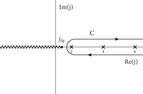
Figure 5: Illustration of the integration contour $\mathbb{C}$ in the complex j-plane used for computing the contour integral (IV.33), with a branch cut displayed for $\text{Re(j)}\leq j_{0g}=2-2/\sqrt{\lambda}$.

Following Brower et al. (2009), we rewrite the sum over even $j=2,4,...$ in (IV.1) as a contour integral in the complex j-plane

$${\cal A}^{LL(quark)}_{\gamma^{*}p\rightarrow\rho^{0}p}(s,t,Q,\epsilon_{L},\epsilon_{L}^{\prime}) \approx -\int_{\mathbb{C}}\frac{dj}{4i}\frac{1+e^{-i\pi j}}{{\rm sin}\pi j}\times\frac{1}{\xi^{j}}\times\frac{1}{\Gamma(\Delta_{g}(j)-2)}\times\mathcal{N}_{q}(j)$$ (IV.33)

$$\times \left(Q_{u}\ \widehat{\mathbb{F}}^{u}_{j(singlet)}(\xi,t;\mu^{2})\,-\,Q_{d}\ \widehat{\mathbb{F}}^{d}_{j(singlet)}(\xi,t;\mu^{2})\right)$$

$$\times e\times f_{V}\times\alpha_{s}(\mu)\times{1\over{Q}}\times\frac{1}{2\sqrt{2}m_{N}}\times\bar{u}(p_{2})u(p_{1})\,,$$

where the contour $\mathbb{C}$, shown in Fig. 5, is at the right most of the branch point of

$$\frac{1}{\Gamma(\Delta_{g}(j)-2)}=\frac{1}{\Gamma\left(\sqrt{2}\lambda^{1/4}(j-j_{0g})^{1/2}\right)}$$

and enclosing the poles at even $j=2,4,...$. Here we have defined

$$\widehat{\mathbb{F}}^{q}_{j(singlet)}(\xi,t;\mu^{2})=\Gamma(\Delta_{g}(j)-2)\times\mathbb{F}^{q}_{j(singlet)}(\xi,t;\mu^{2})$$ (IV.34)

in order to reveal the branch point at $j=j_{0g}=2-2/\sqrt{\lambda}$ coming from our holographic input conformal (Gegenbauer) moments of the gluon GPD at $\mu=\mu_{0}\sim Q_{0}$.

We evaluate the amplitude (IV.33) by wrapping the j-plane contour $\mathbb{C}$ to the left

$${\cal A}^{LL(quark)}_{\gamma^{*}p\rightarrow\rho^{0}p}(s,t,Q,\epsilon_{L},\epsilon_{L}^{\prime}) \approx -\int_{-\infty}^{j_{0g}}\frac{dj}{2i}\frac{1+e^{-i\pi j}}{{\rm sin}\pi j}\times\frac{1}{\xi^{j}}\times\text{Im}\left[\frac{1}{\Gamma(iy)}\right]$$ (IV.35)

$$\times \left(Q_{u}\ \widehat{\mathbb{F}}^{u}_{j(singlet)}(\xi,t;\mu^{2})\,-\,Q_{d}\ \widehat{\mathbb{F}}^{d}_{j(singlet)}(\xi,t;\mu^{2})\right)$$

$$\times \mathcal{N}_{q}(j)\times e\times f_{V}\times\alpha_{s}(\mu)\times{1\over{Q}}\times\frac{1}{2\sqrt{2}m_{N}}\times\bar{u}(p_{2})u(p_{1})\,,$$

with $iy=i\sqrt{2\sqrt{\lambda}(j_{0g}-j)}\,.$ For, $y\rightarrow 0$, we may approximate $\frac{1}{\Gamma(iy)}\approx iy\,e^{i\gamma_{E}y}$ with the Euler constant $\gamma_{E}\approx 0.577216$, and write $\text{Im}\left[\frac{1}{\Gamma(iy)}\right]\approx y\,\text{cos}(\gamma_{E}y)\approx\text{sin}(y)$ for $y\rightarrow 0$ or $j\rightarrow j_{0g}$. Therefore, for $j\rightarrow j_{0g}$, we find

$${\cal A}^{LL(quark)}_{\gamma^{*}p\rightarrow\rho^{0}p}(s,t,Q,\epsilon_{L},\epsilon_{L}^{\prime}) \approx \left(Q_{u}\widehat{\mathbb{F}}^{u}_{j_{0}(singlet)}(\xi,t;\mu^{2})-Q_{d}\widehat{\mathbb{F}}^{d}_{j_{0}(singlet)}(\xi,t;\mu^{2})\right)$$ (IV.36)

$$\times \mathcal{N}_{q}(j_{0g})\times e\,f_{V}\,\alpha_{s}(\mu)\,{1\over{Q}}\,\frac{1}{2\sqrt{2}m_{N}}\,\bar{u}(p_{2})u(p_{1})$$

$$\times -\int_{-\infty}^{j_{0g}}\frac{dj}{2}\frac{1+e^{-i\pi j}}{{\rm sin}\pi j}\times\frac{1}{\xi^{j}}\times\text{sin}\left(\sqrt{2\sqrt{\lambda}(j_{0g}-j)}\right)\,.$$

Real and Imaginary parts
We separate the amplitude (IV.36) into its real and imaginary parts

$${\cal A}^{LL(quark)}_{\gamma^{*}p\rightarrow\rho^{0}p}(s,t,Q,\epsilon_{L},\epsilon_{L}^{\prime})\equiv{\cal A}^{LL(quark)}=\text{Re}\left[{\cal A}^{LL(quark)}\right]+i\text{Im}\left[{\cal A}^{LL(quark)}\right]\,,$$

with

$$\text{Re}\left[{\cal A}^{LL(quark)}\right] = \mathcal{N}_{q}(j_{0g})\times\left(Q_{u}\ \widehat{\mathbb{F}}^{u}_{j_{0q}(singlet)}(\xi,t;\mu^{2})\,-\,Q_{d}\ \widehat{\mathbb{F}}^{d}_{j_{0q}(singlet)}(\xi,t;\mu^{2})\right)$$

$$\times e\,f_{V}\,\alpha_{s}(\mu)\,{1\over{Q}}\,\frac{1}{2\sqrt{2}m_{N}}\,\bar{u}(p_{2})u(p_{1})\times-\int_{-\infty}^{j_{0g}}\frac{dj}{2}\frac{1+\text{cos}\pi j}{{\rm sin}\pi j}\times\frac{1}{\xi^{j}}\times\text{sin}\left(\sqrt{2\sqrt{\lambda}(j_{0g}-j)}\right)\,,$$

$$\text{Im}\left[{\cal A}^{LL(quark)}\right] = \mathcal{N}_{q}(j_{0q})\times\left(Q_{u}\ \widehat{\mathbb{F}}^{u}_{j_{0q}(singlet)}(\xi,t;\mu^{2})\,-\,Q_{d}\ \widehat{\mathbb{F}}^{d}_{j_{0q}(singlet)}(\xi,t;\mu^{2})\right)$$

$$\times e\,f_{V}\,\alpha_{s}(\mu)\,{1\over{Q}}\,\frac{1}{2\sqrt{2}m_{N}}\,\bar{u}(p_{2})u(p_{1})\times\int_{-\infty}^{j_{0g}}\frac{dj}{2}\,\frac{1}{\xi^{j}}\times\text{sin}\left(\sqrt{2\sqrt{\lambda}(j_{0g}-j)}\right)\,.$$

With the change of integration variable $y^{2}=2\sqrt{\lambda}(j_{0g}-j)$, we turn the imaginary part into a Gaussian integral that can be evaluated exactly (with $\tilde{\tau}=\text{log}(1/\xi)$)

$$\text{Im}\left[{\cal A}^{LL(quark)}\right] = \mathcal{N}_{q}(j_{0g})\times\left(Q_{u}\ \widehat{\mathbb{F}}^{u}_{j_{0q}(singlet)}(\xi,t;\mu^{2})\,-\,Q_{d}\ \widehat{\mathbb{F}}^{d}_{j_{0q}(singlet)}(\xi,t;\mu^{2})\right)$$ (IV.38)

$$\times e\,f_{V}\,\alpha_{s}(\mu)\,{1\over{Q}}\,\frac{1}{2\sqrt{2}m_{N}}\,\bar{u}(p_{2})u(p_{1})\times\frac{1}{\xi^{j_{0g}}}\times\int_{-\infty}^{\infty}\frac{dy}{4\pi i\sqrt{\lambda}}\,y\,e^{-\tilde{\tau}y^{2}/2\sqrt{\lambda}}\,e^{iy}\,,$$

$$= \mathcal{N}_{q}(j_{0g})\times\left(Q_{u}\ \widehat{\mathbb{F}}^{u}_{j_{0g}(singlet)}(\xi,t;\mu^{2})\,-\,Q_{d}\ \widehat{\mathbb{F}}^{d}_{j_{0q}(singlet)}(\xi,t;\mu^{2})\right)$$

$$\times e\,f_{V}\,\alpha_{s}(\mu)\,{1\over{Q}}\,\frac{1}{2\sqrt{2}m_{N}}\,\bar{u}(p_{2})u(p_{1})\times\frac{1}{\xi^{j_{0g}}}\times(\sqrt{\lambda}/2\pi)^{1/2}\times\frac{e^{-\sqrt{\lambda}/2\tilde{\tau}}}{\tilde{\tau}^{3/2}}\,.$$

Note the emergence of $1/\xi^{j_{0g}}$ in the imaginary part of the amplitude in (IV.38) with $j_{0g}=2-2/\sqrt{\lambda}$. This follows from the transmutation of the graviton with spin $j=2$, to a Pomeron with spin $j_{0g}$, after Reggeization.

We now compute the real part of the amplitude $\text{Re}\left[{\cal A}^{LL(quark)}\right]$, by first expanding its prefactor near $j=2$

$$\frac{1+\text{cos}\pi j}{{\rm sin}\pi j}\simeq\frac{2}{\pi(j-2)}+\mathcal{O}(j-2)\,,$$ (IV.39)

and establishing the identity $\partial_{\tilde{\tau}}\left[e^{-2\tilde{\tau}}\text{Re}\left[{\cal A}^{LL(quark)}\right]\right]=-(2/\pi)e^{-2\tilde{\tau}}\text{Im}\left[{\cal A}^{LL(quark)}\right]$ which gives us an approximation for the real part

$$\text{Re}\left[{\cal A}^{LL(quark)}\right] \simeq \mathcal{N}_{q}(j_{0g})\times\left(Q_{u}\ \widehat{\mathbb{F}}^{u}_{j_{0q}(singlet)}(\xi,t;\mu^{2})\,-\,Q_{d}\ \widehat{\mathbb{F}}^{d}_{j_{0g}(singlet)}(\xi,t;\mu^{2})\right)$$

$$\times e\,f_{V}\,\alpha_{s}(\mu)\,{1\over{Q}}\,\frac{1}{2\sqrt{2}m_{N}}\,\bar{u}(p_{2})u(p_{1})\times(\sqrt{\lambda}/2\pi)^{1/2}\times\frac{1}{\xi^{2}}\times\int_{\tilde{\tau}}^{\infty}d\tilde{\tau}^{\prime}\,\frac{2e^{-2\tilde{\tau}^{\prime}/\sqrt{\lambda}-\sqrt{\lambda}/2\tilde{\tau}^{\prime}}}{\pi\tilde{\tau}^{\prime 3/2}}\,.$$

Small corrections in the order of $\mathcal{O}(\text{Im}\left[{\cal A}^{LL(quark)}\right]/\text{log}(1/\xi))$ and $\mathcal{O}(\text{Im}\left[{\cal A}^{LL(quark)}\right]/\sqrt{\lambda})$ to (IV.1) can be computed in a standard perturbation series, but can be ignored for $\xi\rightarrow 0$ and fixed large $\sqrt{\lambda}$.

small-$\xi$ Regime
We then compute the integral in (IV.1) in the small-$\xi$ regime, i.e., $\tilde{\tau}=\text{log}(1/\xi)\rightarrow\infty$ at fixed large $\sqrt{\lambda}$, where the integral is dominated by its end point, and can be approximated by

$$\int_{\tilde{\tau}}^{\infty}d\tilde{\tau}^{\prime}\,\frac{2e^{-2\tilde{\tau}^{\prime}/\sqrt{\lambda}-\sqrt{\lambda}/2\tilde{\tau}^{\prime}}}{\pi\tilde{\tau}^{\prime 3/2}}=(\sqrt{\lambda}/\pi)\times e^{-2\tilde{\tau}/\sqrt{\lambda}}\times\frac{e^{-\sqrt{\lambda}/2\tilde{\tau}}}{\tilde{\tau}^{3/2}}\left(1+\mathcal{O}(\sqrt{\lambda}/\tilde{\tau})\right)\,.$$ (IV.41)

Finally, combining this approximation for $\text{Re}\left[{\cal A}^{LL(quark)}\right]$ with the exact result for $\text{Im}\left[{\cal A}^{LL(quark)}\right]$ (IV.38), we find the complex amplitude with evolved singlet quark GPDs (for input gluon GPDs part)

$${\cal A}^{LL(quark)}_{\gamma^{*}p\rightarrow\rho^{0}p}(s,t,Q,\epsilon_{L},\epsilon_{L}^{\prime}) \simeq \Bigg{(}Q_{u}\widehat{\mathbb{F}}^{u}_{j_{0g}(singlet)}(\xi,t;\mu^{2})-Q_{d}\widehat{\mathbb{F}}^{d}_{j_{0g}(singlet)}(\xi,t;\mu^{2})\Bigg{)}$$ (IV.42)

$$\times \Bigg{[}(\sqrt{\lambda}/2\pi)^{1/2}\times\frac{1}{\xi^{2}}\times(\sqrt{\lambda}/\pi)\times e^{-2\tilde{\tau}/\sqrt{\lambda}}\times\frac{e^{-\sqrt{\lambda}/2\tilde{\tau}}}{\tilde{\tau}^{3/2}}$$

$$+ i\times\frac{1}{\xi^{j_{0g}}}\times(\sqrt{\lambda}/2\pi)^{1/2}\times\frac{e^{-\sqrt{\lambda}/2\tilde{\tau}}}{\tilde{\tau}^{3/2}}\Bigg{]}\times\mathcal{N}_{q}(j_{0g})e\,f_{V}\,\alpha_{s}(\mu)\,{1\over{Q}}\,\frac{1}{2\sqrt{2}m_{N}}\,\bar{u}(p_{2})u(p_{1})\,,$$

$$\simeq \Bigg{(}Q_{u}\widehat{\mathbb{F}}^{u}_{j_{0g}(singlet)}(\xi,t;\mu^{2})-Q_{d}\widehat{\mathbb{F}}^{d}_{j_{0g}(singlet)}(\xi,t;\mu^{2})\Bigg{)}$$

$$\times \mathcal{N}_{q}(j_{0g})\times e\,f_{V}\,\alpha_{s}(\mu)\,{1\over{Q}}\,\frac{1}{2\sqrt{2}m_{N}}\,\bar{u}(p_{2})u(p_{1})$$

$$\times \left[\frac{(\sqrt{\lambda}/\pi)}{\xi^{2-2/\sqrt{\lambda}}}+\frac{i}{\xi^{2-2/\sqrt{\lambda}}}\right]\times(\sqrt{\lambda}/2\pi)^{1/2}\times\frac{e^{-\sqrt{\lambda}/2\tilde{\tau}}}{\tilde{\tau}^{3/2}}\,.$$

Therefore, the full complex amplitude due to the evolved singlet quark GPDs is given by (IV.42)

$${\cal A}^{LL(quark)}_{\gamma^{*}p\rightarrow\rho^{0}p}(s,t,Q,\epsilon_{L},\epsilon_{L}^{\prime}) \propto \Bigg{(}Q_{u}\widehat{\mathbb{F}}^{u}_{j_{0g}(singlet)}(\xi,t;\mu^{2})-Q_{d}\widehat{\mathbb{F}}^{d}_{j_{0g}(singlet)}(\xi,t;\mu^{2})\Bigg{)}$$ (IV.43)

$$\times f_{V}\,\alpha_{s}(\mu)\,{1\over{Q}}\,\frac{1}{2\sqrt{2}m_{N}}\,\bar{u}(p_{2})u(p_{1})\times\left[\frac{(\sqrt{\lambda}/\pi)}{\xi^{2-2/\sqrt{\lambda}}}+\frac{i}{\xi^{2-2/\sqrt{\lambda}}}\right]\,,$$

where we have approximated $\mathcal{N}_{q}(j_{0g})\times e\times(\sqrt{\lambda}/2\pi)^{1/2}\times\frac{e^{-\sqrt{\lambda}/2\tilde{\tau}}}{\tilde{\tau}^{3/2}}$ to be a constant since it varies very slowly with $s$.

IV.2 Evolved gluon GPD contribution for $\rho^{0}$

In addition, the electroproduction of neutral rho meson ($\rho^{0}$) in terms of quark DAs and gluon GPDs is given by (see Eq.282 in Diehl (2003))

$$\mathcal{A}^{LL(gluon)}_{\gamma^{*}p\rightarrow\rho^{0}p}(s,t,Q,\epsilon_{L},\epsilon_{L}^{\prime})=$$

$$e\times\frac{1}{8}\times\frac{1}{N_{c}}\times 4\pi\times\alpha_{s}(\mu^{2})\times\frac{1}{Q}\times\left[\int_{0}^{1}dz\,\sum_{q}e_{q}\frac{\Phi^{q}(z)}{z(1-z)}\right]\times\int_{-1}^{1}dx\,\frac{F^{g}(x,\eta,t;\mu^{2})}{x}\left\{\frac{1}{\xi-x-i\epsilon}-\frac{1}{\xi+x-i\epsilon}\right\}\,.$$

On the light front,

$$h^{+}=\bar{u}(p_{2})\gamma^{+}u(p_{1})\approx\frac{p^{+}}{2m_{N}}\times\bar{u}(p_{2})u(p_{1}),$$

and ignoring the Pauli contribution $E^{g}(x,\eta,t;\mu^{2})$ to $F^{g}(x,\eta,t;\mu^{2})$ for $-t\ll 4m_{N}^{2}$, we have

$$F^{g}(x,\eta,t;\mu^{2})\approx\frac{h^{+}}{p^{+}}H^{g}(x,\eta,t;\mu^{2})=H^{g}(x,\eta,t;\mu^{2})\times\frac{1}{2m_{N}}\times\bar{u}(p_{2})u(p_{1})\,,$$ (IV.45)

which simplifies (IV.2)

$$\mathcal{A}^{LL(gluon)}_{\gamma^{*}p\rightarrow\rho^{0}p}(s,t,Q,\epsilon_{L},\epsilon_{L}^{\prime}) = e\times\frac{1}{8}\times\frac{1}{N_{c}}\times\frac{1}{Q}\times 4\pi\times\alpha_{s}(\mu^{2})\times\frac{1}{2m_{N}}\times\bar{u}(p_{2})u(p_{1})$$

$$\times \left[\int_{0}^{1}dz\,\sum_{q}e_{q}\frac{\Phi^{q}(z)}{z(1-z)}\right]\times\int_{0}^{1}dx\,\frac{H^{g}(x,\eta,t;\mu^{2})}{x}\times\left\{\frac{1}{\xi-x-i\epsilon}-\frac{1}{\xi+x-i\epsilon}\right\}\,.$$

Using the conformal expansion of gluon GPDs, the amplitude (IV.2) can be written in terms of the conformal moments of gluon GPDs as

$$\mathcal{A}^{LL(gluon)}_{\gamma^{*}p\rightarrow\rho^{0}p}(s,t,Q,\epsilon_{L},\epsilon_{L}^{\prime})$$

$$= e\times\frac{1}{4}\times\frac{1}{N_{c}}\times\frac{1}{Q}\times\alpha_{s}(\mu^{2})\times\left[\int_{0}^{1}dz\,\sum_{q}e_{q}\frac{\Phi^{q}(z)}{z(1-z)}\right]\times\Bigg{[}\frac{1}{\xi^{2}}\times\int_{0}^{1}dx\,\frac{H^{g}(x,\eta,t;\mu^{2})}{(1-\frac{x^{2}}{\xi^{2}})}$$

$$+ i\pi H^{g}(\xi,\eta,t;\mu^{2})-i\pi H^{g}(-\xi,\eta,t;\mu^{2})\Bigg{]}\times\frac{1}{m_{N}}\times\bar{u}(p_{2})u(p_{1})\,,$$

$$= e\times\frac{1}{4}\times\frac{1}{N_{c}}\times\frac{1}{Q}\times\alpha_{s}(\mu^{2})\times\left[\int_{0}^{1}dz\,\sum_{q}e_{q}\frac{\Phi^{q}(z)}{z(1-z)}\right]\times\frac{1}{m_{N}}\times\bar{u}(p_{2})u(p_{1})$$

$$\times \Bigg{[}\frac{1}{\xi^{2}}\times\sum_{j=2}^{\infty}\frac{1}{\eta^{j-2}}\times\frac{1}{N_{j-2}(\frac{5}{2})}\times\left[\int_{0}^{\eta}\frac{dx}{\eta}\,\frac{\left(1-\frac{x^{2}}{\eta^{2}}\right)^{2}}{(1-\frac{x^{2}}{\xi^{2}})}\times C_{j-2}^{5/2}\left(\frac{x}{\eta}\right)\right]\times\mathbb{F}^{g}_{j}(\eta,t;\mu^{2})$$

$$+ i\pi H^{g}(\xi,\eta,t;\mu^{2})-i\pi H^{g}(-\xi,\eta,t;\mu^{2})\Bigg{]}$$

$$\approx e\times\frac{1}{4}\times\frac{1}{N_{c}}\times\frac{1}{Q}\times\alpha_{s}(\mu^{2})\times\left[\int_{0}^{1}dz\,\sum_{q}e_{q}\frac{\Phi^{q}(z)}{z(1-z)}\right]\times\frac{1}{m_{N}}\times\bar{u}(p_{2})u(p_{1})$$

$$\times \sum_{j=2}^{\infty}\frac{1}{\xi^{j}}\times\frac{1}{N_{j-2}(\frac{5}{2})}\times\left[\int_{0}^{\xi}\frac{dx}{\xi}\,\left(1-\frac{x^{2}}{\xi^{2}}\right)\times C_{j-2}^{5/2}\left(\frac{x}{\xi}\right)\right]\times\mathbb{F}^{g}_{j}(\xi,t;\mu^{2})\,,$$

in the last line we have used $\eta\sim\xi$. Note that the $i\pi H^{g}$ contribution vanishes for $\xi=\pm\eta$. We can rewrite (IV.2) more compactly as

$$\mathcal{A}^{LL(gluon)}_{\gamma^{*}p\rightarrow\rho^{0}p}(s,t,Q,\epsilon_{L},\epsilon_{L}^{\prime}) \approx e\times f_{V}^{\prime}\times\alpha_{s}(\mu^{2})\times{1\over{Q}}\times\sum_{j=2}^{\infty}\frac{1}{\xi^{j}}\times\mathcal{N}_{g}(j)\times\mathbb{F}^{g}_{j}(\xi,t;\mu^{2})\times\frac{1}{2\sqrt{2}m_{N}}\times\bar{u}(p_{2})u(p_{1})\,,$$

where we have defined

$$\mathcal{N}_{g}(j) \equiv \frac{1}{4}\times\frac{1}{N_{c}}\times 2\sqrt{2}\times\frac{1}{N_{j-2}(\frac{5}{2})}\times I_{g}(j)\,,$$ (IV.49)

and the integrals ($\tilde{x}=x/\xi$)

$$f_{V}^{\prime}=\int_{0}^{1}dz\,\sum_{q}e_{q}\frac{\Phi^{q}(z)}{z(1-z)}\,,\qquad\qquad I_{g}(j)=\int_{0}^{1}d\tilde{x}\,\left(1-\tilde{x}^{2}\right)C_{j-2}^{5/2}\left(\tilde{x}\right)\,.$$ (IV.50)

The resummation by j-contour for the gluon GPD contribution (IV.2) is similar to the resummation for the singlet quark GPDs, and the detailed derivation is given in Appendix F. Here we only provide the final answer.

After the resummation by j-contour, the full complex amplitude due to the evolved gluon GPD is given by (F.241) i.e.,

$${\cal A}^{LL(gluon)}_{\gamma^{*}p\rightarrow\rho^{0}p}(s,t,Q,\epsilon_{L},\epsilon_{L}^{\prime}) \propto \widehat{\mathbb{F}}^{g}_{j_{0g}}(\xi,t;\mu^{2})\times e\,f_{V}^{\prime}\,\alpha_{s}(\mu)\,{1\over{Q}}\,\frac{1}{2\sqrt{2}m_{N}}\,\bar{u}(p_{2})u(p_{1})$$ (IV.51)

$$\times \frac{1}{\xi^{2-2/\sqrt{\lambda}}}\times\left[(\sqrt{\lambda}/\pi)+i\right]\,,$$

with $j_{0g}=2-2/\sqrt{\lambda}$, and $\tilde{\tau}=\text{log}(1/\xi)$. We have also approximated $\mathcal{N}_{g}(j_{0g})\times e\times(\sqrt{\lambda}/2\pi)^{1/2}\times\frac{e^{-\sqrt{\lambda}/2\tilde{\tau}}}{\tilde{\tau}^{3/2}}$ to be a constant (that will be fixed by experimental data) since it varies slowly with $s$.

IV.3 Total quark and gluon GPDs contribution to the electroproduction of $\rho^{0}$

To summarize, we have found the singlet quark GPD contribution to the $\rho^{0}$ amplitude to be given by

$${\cal A}^{LL(quark)}_{\gamma^{*}p\rightarrow\rho^{0}p}(s,t,Q,\epsilon_{L},\epsilon_{L}^{\prime}) \propto \Bigg{(}Q_{u}\widehat{\widehat{\mathbb{F}}}^{u}_{j_{0g}(singlet)}(\xi,t;\mu^{2})-Q_{d}\widehat{\widehat{\mathbb{F}}}^{d}_{j_{0g}(singlet)}(\xi,t;\mu^{2})\Bigg{)}$$ (IV.52)

$$\times f_{V}\,\alpha_{s}(\mu)\,{1\over{Q}}\,\frac{1}{2\sqrt{2}m_{N}}\,\bar{u}(p_{2})u(p_{1})\times\left[\frac{(\sqrt{\lambda}/\pi)}{\xi^{2-2/\sqrt{\lambda}}}+\frac{i}{\xi^{2-2/\sqrt{\lambda}}}\right]$$

$$\propto {\cal A}^{quark}_{\rho^{0}}(s,t,Q)\times\frac{1}{2\sqrt{2}m_{N}}\,\bar{u}(p_{2})u(p_{1})\,,$$

where we have normalized the singlet quark conformal moments using the lattice data from Hagler et al. (2008) as

$$\widehat{\widehat{\mathbb{F}}}^{u+d}_{j(singlet)}(\xi,t;\mu^{2}) = 0.526\times\frac{\widehat{\mathbb{F}}^{u+d}_{j(singlet)}(\xi,t;\mu^{2})}{\widehat{\mathbb{F}}^{u+d}_{j=2(singlet)}(\xi=0,t=0;\mu^{2}=4~{}\text{GeV}^{2})}$$ (IV.53)

$$\widehat{\widehat{\mathbb{F}}}^{u-d}_{j(singlet)}(\xi,t;\mu^{2}) = 0.210\times\frac{\widehat{\mathbb{F}}^{u-d}_{j(singlet)}(\xi,t;\mu^{2})}{\widehat{\mathbb{F}}^{u-d}_{j=2(singlet)}(\xi=0,t=0;\mu^{2}=4~{}\text{GeV}^{2})}\,,$$ (IV.54)

with $\widehat{\mathbb{F}}^{u\pm d}_{j(singlet)}(\xi,t;\mu^{2})=\Gamma(\Delta_{g}(j)-2)\times\mathbb{F}^{u\pm d}_{j(singlet)}(\xi,t;\mu^{2})$ which is given in (III.21). Note that we have used the average value of $A_{2}^{u+d}(-t=0)=\widehat{\widehat{\mathbb{F}}}^{u+d}_{j=2(singlet)}(\xi=0,t=0;\mu^{2}=4~{}\text{GeV}^{2})=0.526$ from Table XV and Table XVI of Hagler et al. (2008). We have also used the average value of $A_{2}^{u-d}(-t=0)=\widehat{\widehat{\mathbb{F}}}^{u-d}_{j=2(singlet)}(\xi=0,t=0;\mu^{2}=4~{}\text{GeV}^{2})=0.210$ from Table IX and Table X of Hagler et al. (2008). Also note that we have

$$\widehat{\widehat{\mathbb{F}}}^{u}_{j(singlet)}(\xi,t;\mu^{2}) = \frac{1}{2}\times\left(\widehat{\widehat{\mathbb{F}}}^{u+d}_{j(singlet)}(\xi,t;\mu^{2})+\widehat{\widehat{\mathbb{F}}}^{u-d}_{j(singlet)}(\xi,t;\mu^{2})\right)$$ (IV.55)

$$\widehat{\widehat{\mathbb{F}}}^{d}_{j(singlet)}(\xi,t;\mu^{2}) = \frac{1}{2}\times\left(\widehat{\widehat{\mathbb{F}}}^{u+d}_{j(singlet)}(\xi,t;\mu^{2})-\widehat{\widehat{\mathbb{F}}}^{u-d}_{j(singlet)}(\xi,t;\mu^{2})\right)\,.$$ (IV.56)

We have also found the gluon GPD contribution to the $\rho^{0}$ amplitude to be

$${\cal A}^{LL(gluon)}_{\gamma^{*}p\rightarrow\rho^{0}p}(s,t,Q,\epsilon_{L},\epsilon_{L}^{\prime}) \propto \widehat{\widehat{\mathbb{F}}}^{g}_{j_{0g}}(\xi,t;\mu^{2})\times f_{V}^{\prime}\,\alpha_{s}(\mu)\,{1\over{Q}}\,\frac{1}{2\sqrt{2}m_{N}}\,\bar{u}(p_{2})u(p_{1})$$ (IV.57)

$$\times \left[\frac{(\sqrt{\lambda}/\pi)}{\xi^{2-2/\sqrt{\lambda}}}+\frac{i}{\xi^{2-2/\sqrt{\lambda}}}\right]$$

$$\propto {\cal A}^{gluon}_{\rho^{0}}(s,t,Q)\times\frac{1}{2\sqrt{2}m_{N}}\,\bar{u}(p_{2})u(p_{1})\,,$$

with $j_{0g}=2-2/\sqrt{\lambda}$, $\tilde{\tau}=\text{log}(1/\xi)$, $f_{V}^{\prime}\approx f_{V}$, and we have normalized the gluonic conformal moments using the lattice data from Hagler et al. (2008) as

$$\widehat{\widehat{\mathbb{F}}}^{g}_{j}(\xi,t;\mu^{2})=0.474\times\frac{\widehat{\mathbb{F}}^{g}_{j}(\xi,t;\mu^{2})}{\widehat{\mathbb{F}}^{g}_{j=2}(\xi=0,t=0;\mu^{2}=4~{}\text{Gev}^{2})}$$ (IV.58)

where $\widehat{\mathbb{F}}^{g}_{j}(\xi,t;\mu^{2})=\Gamma(\Delta_{g}(j)-2)\times\mathbb{F}^{g}_{j}(\xi,t;\mu^{2})$ is given in (III.22). Note that we have used the fact that $A_{2}^{g}(-t=0)=\widehat{\widehat{\mathbb{F}}}^{g}_{j=2}(\xi=0,t=0;\mu^{2}=4~{}\text{Gev}^{2})=1-A_{2}^{u+d}(-t=0)=1-\widehat{\widehat{\mathbb{F}}}^{u+d}_{j=2(singlet)}(\xi=0,t=0;\mu^{2}=4~{}\text{GeV}^{2})=1-0.526=0.474$ from Hagler et al. (2008).

IV.4 s+u-channel contribution to the electroproduction of $\rho^{0}$

In this section, we first compute the $s+u$-channel contribution to DVCS, shown in Fig. 6a, and generalize the result to determine the s+u-channel contribution to the electroproduction of $\rho^{0}$, shown in Fig. 6b. See (IV.4.3) for the final answer to $\rho^{0}$ electroproduction.

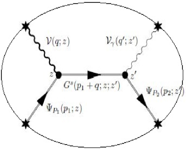
(a)

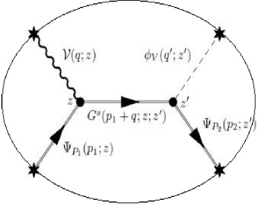
(b)

Figure 6: (a) Holographic s-channel contribution to the electroproduction of a photon (DVCS). (b) Holographic s-channel contribution to the electroproduction of a vector meson.

The holographic DVCS amplitude shown in Fig. 6a involves the bulk Dirac fields

$$\Psi_{1p_{1}/2p_{1}}(z)=\left(\psi_{R}(z)P_{\pm}+\psi_{L}(z)P_{\mp}\right)\times u(p_{1})$$

$$\bar{\Psi}_{1p_{2}/2p_{2}}(z^{\prime})=\bar{u}(p_{2})\times\left(\psi_{R}(z^{\prime})P_{\mp}+\psi_{L}(z^{\prime})P_{\pm}\right)$$

$$\Psi_{1p/2p}(z)\equiv\Psi_{1/2}(p,z;n=0)$$

$$\psi_{R/L}(z)\equiv\psi_{R/L}(z;n=0)\,.$$

To proceed, we define

$$\tilde{G}^{s}(p_{1}+q,M_{n_{x}})=iG^{s}(p_{1}+q,M_{n_{x}})=\frac{i(p/_{1}+q/+M_{n_{x}})}{(p_{1}+q)^{2}-M_{n_{x}}^{2}+i\epsilon}$$

in terms of which the Dirac contribution to the s-channel is

$$i\epsilon_{\mu}\epsilon_{\nu}^{\prime*}T_{s(\text{Dirac})}^{\mu\nu}(s,t;Q^{2},Q^{\prime 2})=\sum_{n_{x}}i\epsilon_{\mu}\epsilon_{\nu}^{\prime*}T_{s(\text{Dirac})}^{\mu\nu}(n_{x},s,t;Q^{2},Q^{\prime 2})$$

$$i\epsilon_{\mu}\epsilon_{\nu}^{\prime*}T_{s(\text{Dirac})}^{\mu\nu}(n_{x},s,t;Q^{2},Q^{\prime 2})=\int dz\sqrt{g}e^{-\tilde{\kappa}^{2}z^{2}}\,\frac{z}{R}\int dz^{\prime}\sqrt{g^{\prime}}e^{-\tilde{\kappa}^{2}z^{\prime 2}}\,\frac{z^{\prime}}{R}$$

$$\times\bar{\Psi}_{1p_{2}}(z^{\prime})\times\left(-i\gamma^{\nu}\right)\times\Big{(}\frac{1}{3}V_{\nu}^{0}(q^{\prime}z^{\prime})T^{0}+V_{\nu}^{3}(q^{\prime}z^{\prime})T^{3}\Big{)}\times\Big{(}\psi_{R}(z^{\prime};n_{x})P_{+}+\psi_{L}(z^{\prime};n_{x})P_{-}\Big{)}$$

$$\times\tilde{G}^{s}(p_{1}+q,M_{n_{x}})\times\Big{(}\psi_{R}(z;n_{x})P_{-}+\psi_{L}(z;n_{x})P_{+}\Big{)}\times\left(-i\gamma^{\mu}\right)\times\Big{(}\frac{1}{3}V_{\mu}^{0}(qz)T^{0}+V_{\mu}^{3}(qz)T^{3}\Big{)}\Psi_{1p_{1}}(z)$$

$$+ \int dz\sqrt{g}e^{-\tilde{\kappa}^{2}z^{2}}\,\frac{z}{R}\int dz^{\prime}\sqrt{g^{\prime}}e^{-\tilde{\kappa}^{2}z^{\prime 2}}\,\frac{z^{\prime}}{R}$$

$$\times\bar{\Psi}_{2p_{2}}(z^{\prime})\times\left(-i\gamma^{\nu}\right)\times\Big{(}\frac{1}{3}V_{\nu}^{0}(q^{\prime}z^{\prime})T^{0}+V_{\nu}^{3}(q^{\prime}z^{\prime})T^{3}\Big{)}\times\Big{(}\psi_{R}(z^{\prime};n_{x})P_{-}+\psi_{L}(z^{\prime};n_{x})P_{+}\Big{)}$$

$$\times\tilde{G}^{s}(p_{1}+q,M_{n_{x}})\times\Big{(}\psi_{R}(z;n_{x})P_{+}+\psi_{L}(z;n_{x})P_{-}\Big{)}\times\left(-i\gamma^{\mu}\right)\times\Big{(}\frac{1}{3}V_{\mu}^{0}(qz)T^{0}+V_{\mu}^{3}(qz)T^{3}\Big{)}\Psi_{2p_{1}}(z)\,,$$

Setting $q^{2}=-Q^{2}$, we have $\frac{1}{3}V_{\mu}^{0}(qz)T^{0}+V_{\mu}^{3}(qz)T^{3}=\epsilon_{\mu}\times\frac{1}{2}\mathcal{V}(Qz)$ for the proton, we have

$$i\epsilon_{\mu}\epsilon_{\nu}^{\prime*}T_{s(\text{Dirac})}^{\mu\nu}(n_{x},s,t;Q^{2},Q^{\prime 2})=\int dz\sqrt{g}e^{-\tilde{\kappa}^{2}z^{2}}\,\frac{z}{R}\int dz^{\prime}\sqrt{g^{\prime}}e^{-\tilde{\kappa}^{2}z^{\prime 2}}\,\frac{z^{\prime}}{R}$$

$$\times\bar{u}(p_{2})\times\left(-i\gamma^{\nu}\right)\times\epsilon_{\nu}^{\prime*}\mathcal{V}(Q^{\prime}z^{\prime})\times\frac{1}{2}\Big{(}\psi_{R}(z^{\prime})\psi_{R}(z^{\prime};n_{x})P_{+}+\psi_{L}(z^{\prime})\psi_{L}(z^{\prime};n_{x})P_{-}\Big{)}$$

$$\times\tilde{G}^{s}(p_{1}+q,M_{n_{x}})\times\left(-i\gamma^{\mu}\right)\times\frac{1}{2}\Big{(}\psi_{R}(z;n_{x})\psi_{R}(z)P_{+}+\psi_{L}(z;n_{x})\psi_{L}(z)P_{-}\Big{)}\times\epsilon_{\mu}\mathcal{V}(Qz)\times u(p_{1})$$

$$+ \int dz\sqrt{g}e^{-\tilde{\kappa}^{2}z^{2}}\,\frac{z}{R}\int dz^{\prime}\sqrt{g^{\prime}}e^{-\tilde{\kappa}^{2}z^{\prime 2}}\,\frac{z^{\prime}}{R}$$

$$\times\bar{u}(p_{2})\times\left(-i\gamma^{\nu}\right)\times\epsilon_{\nu}^{\prime*}\mathcal{V}(Q^{\prime}z^{\prime})\times\frac{1}{2}\Big{(}\psi_{R}(z^{\prime})\psi_{R}(z^{\prime};n_{x})P_{-}+\psi_{L}(z^{\prime})\psi_{L}(z^{\prime};n_{x})P_{+}\Big{)}$$

$$\times\tilde{G}^{s}(p_{1}+q,M_{n_{x}})\times\left(-i\gamma^{\mu}\right)\times\frac{1}{2}\Big{(}\psi_{R}(z;n_{x})\psi_{R}(z)P_{-}+\psi_{L}(z;n_{x})\psi_{L}(z)P_{+}\Big{)}\times\epsilon_{\mu}\mathcal{V}(Qz)\times u(p_{1})$$

$$= \bar{u}(p_{2})\times\epsilon_{\nu}^{\prime*}\times\frac{1}{2}\Big{(}\mathcal{I}_{R}(Q^{\prime},n_{x})P_{-}+\mathcal{I}_{L}(Q^{\prime},n_{x})P_{+}\Big{)}\times\left(-i\gamma^{\nu}\right)\times\tilde{G}^{s}(p_{1}+q,M_{n_{x}})\times\left(-i\gamma^{\mu}\right)$$

$$\times \frac{1}{2}\Big{(}\mathcal{I}_{R}(Q,n_{x})P_{+}+\mathcal{I}_{L}(Q,n_{x})P_{-}\Big{)}\times\epsilon_{\mu}\times u(p_{1})$$

$$+ \bar{u}(p_{2})\times\epsilon_{\nu}^{\prime*}\times\frac{1}{2}\Big{(}\mathcal{I}_{R}(Q^{\prime},n_{x})P_{+}+\mathcal{I}_{L}(Q^{\prime},n_{x})P_{-}\Big{)}\times\left(-i\gamma^{\nu}\right)\times\tilde{G}^{s}(p_{1}+q,M_{n_{x}})\times\left(-i\gamma^{\mu}\right)$$

$$\times \frac{1}{2}\Big{(}\mathcal{I}_{R}(Q,n_{x})P_{-}+\mathcal{I}_{L}(Q,n_{x})P_{+}\Big{)}\times\epsilon_{\mu}\times u(p_{1})$$

or more explicitly

$$= \bar{u}(p_{2})\times\epsilon_{\nu}^{\prime*}\times\left(-i\gamma^{\nu}\right)\times\,iG_{1}^{s}(p_{1}+q,M_{n_{x}})\times\left(-i\gamma^{\mu}\right)\times\epsilon_{\mu}$$

$$\times\frac{1}{4}\Big{(}\mathcal{I}_{R}(Q^{\prime},n_{x})\mathcal{I}_{R}(Q,n_{x})P_{+}+\mathcal{I}_{L}(Q^{\prime},n_{x})\mathcal{I}_{L}(Q,n_{x})P_{-}\Big{)}\times u(p_{1})$$

$$+ \bar{u}(p_{2})\times\epsilon_{\nu}^{\prime*}\times\left(-i\gamma^{\nu}\right)\times\,iG_{2}^{s}(p_{1}+q,M_{n_{x}})\times\left(-i\gamma^{\mu}\right)\times\epsilon_{\mu}$$

$$\times\frac{1}{4}\Big{(}\mathcal{I}_{R}(Q^{\prime},n_{x})\mathcal{I}_{L}(Q,n_{x})P_{-}+\mathcal{I}_{L}(Q^{\prime},n_{x})\mathcal{I}_{R}(Q,n_{x})P_{+}\Big{)}\times u(p_{1})$$

$$+ \bar{u}(p_{2})\times\epsilon_{\nu}^{\prime*}\times\left(-i\gamma^{\nu}\right)\times\,iG_{1}^{s}(p_{1}+q,M_{n_{x}})\times\left(-i\gamma^{\mu}\right)\times\epsilon_{\mu}$$

$$\times\frac{1}{4}\Big{(}\mathcal{I}_{R}(Q^{\prime},n_{x})\mathcal{I}_{R}(Q,n_{x})P_{-}+\mathcal{I}_{L}(Q^{\prime},n_{x})\mathcal{I}_{L}(Q,n_{x})P_{+}\Big{)}\times u(p_{1})$$

$$+ \bar{u}(p_{2})\times\epsilon_{\nu}^{\prime*}\times\left(-i\gamma^{\nu}\right)\times\,iG_{2}^{s}(p_{1}+q,M_{n_{x}})\times\left(-i\gamma^{\mu}\right)\times\epsilon_{\mu}$$

$$\times\frac{1}{4}\Big{(}\mathcal{I}_{R}(Q^{\prime},n_{x})\mathcal{I}_{L}(Q,n_{x})P_{+}+\mathcal{I}_{L}(Q^{\prime},n_{x})\mathcal{I}_{R}(Q,n_{x})P_{-}\Big{)}\times u(p_{1})$$

$$= \bar{u}(p_{2})\times\epsilon_{\nu}^{\prime*}\times\left(-i\gamma^{\nu}\right)\times\,iG_{1}^{s}(p_{1}+q,M_{n_{x}})\times\left(-i\gamma^{\mu}\right)\times\epsilon_{\mu}$$

$$\times\frac{1}{4}\Big{(}\mathcal{I}_{R}(Q^{\prime},n_{x})\mathcal{I}_{R}(Q,n_{x})+\mathcal{I}_{L}(Q^{\prime},n_{x})\mathcal{I}_{L}(Q,n_{x})\Big{)}\times u(p_{1})$$

$$+ \bar{u}(p_{2})\times\epsilon_{\nu}^{\prime*}\times\left(-i\gamma^{\nu}\right)\times\,iG_{2}^{s}(p_{1}+q,M_{n_{x}})\times\left(-i\gamma^{\mu}\right)\times\epsilon_{\mu}$$

$$\times\frac{1}{4}\Big{(}\mathcal{I}_{R}(Q^{\prime},n_{x})\mathcal{I}_{L}(Q,n_{x})+\mathcal{I}_{L}(Q^{\prime},n_{x})\mathcal{I}_{R}(Q,n_{x})\Big{)}\times u(p_{1})\,,$$

where we have used the identities $P_{\pm}^{2}=P_{\pm}$, $P_{\pm}P_{\mp}=0$, and $\gamma^{\mu}P_{\pm}=P_{\mp}\gamma^{\mu}$, and we have defined

$$\tilde{G}^{s}(p_{1}+q,M_{n_{x}})=\frac{i(p/_{1}+q/+M_{n_{x}})}{(p_{1}+q)^{2}-M_{n_{x}}^{2}+i\epsilon}=\,iG_{1}^{s}(p_{1}+q,M_{n_{x}})\,+\,iG_{2}^{s}(p_{1}+q,M_{n_{x}})$$ (IV.64)

with

$$G_{1}^{s}(p_{1}+q,M_{n_{x}}) = \frac{(p/_{1}+q/)}{(p_{1}+q)^{2}-M_{n_{x}}^{2}+i\epsilon}$$

$$G_{2}^{s}(p_{1}+q,M_{n_{x}}) = \frac{M_{n_{x}}}{(p_{1}+q)^{2}-M_{n_{x}}^{2}+i\epsilon}\,,$$ (IV.65)

we have also dropped the longitudinal contributions by assuming $\epsilon\cdot q=\epsilon^{\prime}\cdot q^{\prime}=0$.

Finally, after some simplification, we find

$$\epsilon_{\mu}\epsilon_{\nu}^{\prime*}T_{s(\text{Dirac})}^{\mu\nu}(s,t;Q^{2},Q^{\prime 2})$$

$$=-\sum_{n_{x}}\bigg{[}\bar{u}(p_{2})\times\epsilon_{\nu}^{\prime*}\times\gamma^{\nu}\times G_{1}^{s}(p_{1}+q,M_{n_{x}})\times\gamma^{\mu}\times\epsilon_{\mu}$$

$$\times\frac{1}{2}\Big{(}\mathcal{I}_{R}(Q^{\prime},n_{x})\mathcal{I}_{R}(Q,n_{x})+\mathcal{I}_{L}(Q^{\prime},n_{x})\mathcal{I}_{L}(Q,n_{x})\Big{)}\times u(p_{1})$$

$$\qquad\qquad+\bar{u}(p_{2})\times\epsilon_{\nu}^{\prime*}\times\gamma^{\nu}\times G_{2}^{s}(p_{1}+q,M_{n_{x}})\times\gamma^{\mu}\times\epsilon_{\mu}$$

$$\times\frac{1}{2}\Big{(}\mathcal{I}_{R}(Q^{\prime},n_{x})\mathcal{I}_{L}(Q,n_{x})+\mathcal{I}_{L}(Q^{\prime},n_{x})\mathcal{I}_{R}(Q,n_{x})\Big{)}\times u(p_{1})\bigg{]}\,.$$

for transverse $\epsilon,\epsilon^{\prime}$ polarizations. For $Q^{\prime 2}=0$, the sum is dominated by the ground state since $\mathcal{I}_{R/L}(Q^{\prime}=0,n_{x})=\delta_{0,n_{x}}$, and we find

$$T_{s(\text{Dirac})}^{\mu\nu}(s,t;Q^{2}) = -\bar{u}(p_{2})\times\gamma^{\nu}\times G_{1}^{s}(p_{1}+q,M_{0})\times\gamma^{\mu}\times\frac{1}{2}\Big{(}\mathcal{I}_{R}(Q,0)+\mathcal{I}_{L}(Q,0)\Big{)}\times u(p_{1})$$

$$+\bar{u}(p_{2})\times\gamma^{\nu}\times G_{2}^{s}(p_{1}+q,M_{0})\times\gamma^{\mu}\times\frac{1}{2}\Big{(}\mathcal{I}_{L}(Q,0)+\mathcal{I}_{R}(Q,0)\Big{)}\times u(p_{1})\,,$$

$$= -C_{1}(Q)\times\bar{u}(p_{2})\times\gamma^{\nu}\times G^{s}(p_{1}+q,M_{0})\times\gamma^{\mu}\times u(p_{1})\,.$$

Including the Pauli contribution in similar fashion, we find

$$\epsilon_{\mu}\epsilon_{\nu}^{\prime*}T_{s}^{\mu\nu}(s,t;Q^{2}) = -\epsilon_{\mu}\epsilon_{\nu}^{\prime*}\times\bar{u}(p_{2})\times\gamma^{\nu}\times G^{s}(p_{1}+q,M_{0})\times\gamma^{\mu}\times\left(F_{1}(Q)-F_{2}(Q)\frac{\not{q}}{2M_{0}}\right)\times u(p_{1})\,,$$

where we have also ignored the longitudinal contribution (by imposing $\epsilon\cdot q=0$) in order to write

$$\epsilon_{\mu}\times\sigma^{\mu\nu}q_{\nu}=\epsilon_{\mu}\times i\left(\gamma^{\mu}\gamma^{\nu}-\eta^{\mu\nu}\right)q_{\nu}=\epsilon_{\mu}\times i\gamma^{\mu}\not{q}$$

The holographic proton Dirac and Pauli form factors $F_{1,2}(Q)$ are given in (IV.4.2). The u-channel contribution follows by inspection

$$\epsilon_{\mu}\epsilon_{\nu}^{\prime*}T_{u}^{\mu\nu}(s,t;Q^{2}) = -\epsilon_{\mu}\epsilon_{\nu}^{\prime*}\times\bar{u}(p_{2})\times\gamma^{\mu}\times\left(F_{1}^{P}(Q)-F_{2}^{P}(Q)\frac{\not{q}}{2M_{0}}\right)\times G^{u}(p_{1}-q,M_{0})\times\gamma^{\nu}\times u(p_{1})\,.$$

IV.4.1 High-energy limit

In the high energy limit $(s,u\gg M_{0}^{2})$ we can ignore the target mass, and $G^{s,u}$ simplify

$$G^{s}(p_{1}+q,M_{0}) = \frac{p/_{1}+q/+M_{0}}{(p_{1}+q)^{2}-M_{0}^{2}+i\epsilon}\approx\frac{p/_{1}+q/}{(p_{1}+q)^{2}+i\epsilon}\,,$$

$$G^{u}(p_{1}-q,M_{0}) = \frac{p/_{1}-q/+M_{0}}{(p_{1}-q)^{2}-M_{0}^{2}+i\epsilon}\approx\frac{p/_{1}-q/}{(p_{1}-q)^{2}+i\epsilon}\,.$$ (IV.70)

Using the light-cone kinematics Belitsky and Radyushkin (2005)

$$\frac{1}{(p_{1}+q)^{2}+i\epsilon}\approx\frac{1}{(p\cdot\tilde{q})}\frac{1}{1-\xi+i\epsilon}\,,$$ (IV.71)

with $\xi$ the longitudinal momentum transfer or skewness, and the spin reduction (for $p_{\perp}=p_{x,y}=0$) Belitsky and Radyushkin (2005)

$$\gamma^{\mu}G^{s}(p_{1}+q,M_{0})\gamma^{\nu}\simeq\frac{1}{(p\cdot\tilde{q})(1-\xi+i\epsilon)}\Bigg{[}S^{\mu\nu;\rho\sigma}\left(\frac{1}{2}(p\cdot\tilde{q})n_{\sigma}+\frac{1}{2}(1-\xi)p_{\sigma}\right)\gamma_{\rho}+i\varepsilon^{\mu\nu\rho\sigma}\left(\frac{1}{2}p_{\sigma}+\tilde{q}_{\sigma}\right)\gamma_{\rho}\gamma^{5}\Bigg{]}\,.$$

we have for the $s+u$-contribution

$$T^{\mu\nu}_{s+u} = -\bar{u}(p_{2})\times\left[\gamma^{\mu}G^{s}(p_{1}+q,M_{0})\gamma^{\nu}+\gamma^{\nu}G^{u}(p_{1}-q,M_{0})\gamma^{\mu}\right]\times\left(F_{1}^{P}(Q)-F_{2}^{P}(Q)\frac{q/}{2M_{0}}\right)\times u(p_{1})$$

$$= \!\!\!\frac{1}{2p\cdot\tilde{q}}\,C^{p[-]}_{(0)}(\xi)\left\{(p\cdot\tilde{q})S^{\mu\nu;\rho\sigma}n_{\sigma}F^{p}_{\rho}(Q)+i\varepsilon^{\mu\nu\rho\sigma}p_{\sigma}\,\widetilde{F}^{p}_{\rho}(Q)\right\}+\frac{1}{2p\cdot\tilde{q}}C^{p[+]}_{(0)}(\xi)\left\{2i\varepsilon^{\mu\nu\rho\sigma}\tilde{q}_{\sigma}\widetilde{F}^{p}_{\rho}(Q)\right\}$$

$$\,,$$ (IV.72)

We have defined the spin structure

$$S^{\mu\nu;\rho\sigma}\equiv\eta^{\mu\rho}\eta^{\nu\sigma}+\eta^{\mu\sigma}\eta^{\nu\rho}-\eta^{\mu\nu}\eta^{\rho\sigma}$$

and the sum of the ratios

$$C^{p[\pm]}_{(0)}(\xi)=\frac{1}{\xi-1-i\epsilon}\pm\frac{1}{\xi+1-i\epsilon}$$ (IV.73)

The vector and axial form factors are

$$F^{p}_{\rho}(Q)=p_{\rho}\left(\frac{h^{+}}{p^{+}}F_{1}^{P}(Q)+\frac{e^{+}}{p^{+}}F_{2}^{P}(Q)\right)=p_{\rho}\times F^{p}(Q)\,,$$

$$\widetilde{F}^{p}_{\rho}(Q)=p_{\rho}\left(\frac{\widetilde{h}^{+}}{p^{+}}F_{1}^{P}(Q)+\frac{\widetilde{e}^{+}}{p^{+}}F_{2}^{P}(Q)\right)=p_{\rho}\times\widetilde{F}^{p}(Q)\,.$$

respectively, with the Dirac bilinears

$$e^{\mu} = \frac{t^{\nu\mu}\tilde{q}_{\nu}}{2M_{0}}\,,\qquad\widetilde{e}^{\mu}=\frac{\widetilde{t}^{\nu\mu}\tilde{q}_{\nu}}{2M_{0}}\,.$$ (IV.75)

and the nucleon matrix elements

$$\begin{array}[]{ll}b=\bar{u}(p_{2})u(p_{1})\,,&\widetilde{b}=\bar{u}(p_{2})\gamma^{5}u(p_{1})\,,\\ h^{\mu}=\bar{u}(p_{2})\gamma^{\mu}u(p_{1})\,,&\widetilde{h}^{\mu}=\bar{u}(p_{2})\gamma^{\mu}\gamma^{5}u(p_{1})\,,\\ t^{\mu\nu}=\bar{u}(p_{2})i\sigma^{\mu\nu}u(p_{1})\,,&\widetilde{t}^{\mu\nu}=\bar{u}(p_{2})i\sigma^{\mu\nu}\gamma^{5}u(p_{1})\,,\end{array}$$ (IV.76)

IV.4.2 TT and LL s+u-channel holographic DVCS amplitude

Contracting the $s+u$-channel holographic amplitude $T_{s+u}^{\mu\nu}$ with the transverse polariztion tensors $\epsilon_{T\mu}$ and $\epsilon_{T\nu}^{\prime*}$, we find

$$\epsilon_{T\mu}\epsilon_{T\nu}^{\prime*}T_{s+u}^{\mu\nu}(s,t;Q^{2})=-\epsilon_{T}\cdot\epsilon_{T}^{\prime}\times\left[\frac{1}{2}C^{p[-]}_{(0)}(\xi)\times F^{p}(Q)\right]\,.$$

Similarly, contracting the $s+u$-channel holographic amplitude $T_{s+u}^{\mu\nu}$ with the longitudinal polarization tensors $\epsilon_{L\mu}$ and $\epsilon_{L\nu}^{\prime*}$, we find

$$\epsilon_{L\mu}\epsilon_{L\nu}^{\prime*}T_{s+u}^{\mu\nu}(s,t;Q^{2})=-\epsilon_{L}\cdot\epsilon_{L}^{\prime}\times\left[\frac{1}{2}C^{p[-]}_{(0)}(\xi)\times F^{p}(Q)\right]\,.$$

We will also use the approximation

$$h^{+}=\bar{u}(p_{2})\gamma^{+}u(p_{1})\approx\frac{p^{+}}{2m_{N}}\times\bar{u}(p_{2})u(p_{1})\,,$$ (IV.79)

and our holographic electromagnetic form factors $F_{1,2}^{P}(Q)$

$$F_{1}^{P}(Q) = \left(\frac{a_{Q}}{2}+\tau_{N}\right)\times B(\tau_{N},a_{Q}+1)+0.448\times\frac{a_{Q}(a_{Q}(\tau_{N}-1)-1)}{(a_{Q}+\tau_{N})(a_{Q}+\tau_{N}+1)}\times B(\tau_{N}-1,a_{Q}+1)\,,$$

$$F_{2}^{P}(Q) = 1.793\times\tau_{N}\times B(\tau_{N},a_{Q}+1)\,,$$

$$F_{1}^{N}(Q) = -0.478\times\frac{a_{Q}(a_{Q}(\tau_{N}-1)-1)}{(a_{Q}+\tau_{N}+1)(a_{Q}+\tau_{N})}\times B(\tau_{N}-1,a_{Q}+1)\,,$$

$$F_{2}^{N}(Q) = -1.913\times\tau_{N}\times B(\tau_{N},a_{Q}+1)\,,$$

where $a_{Q}=Q^{2}/4\kappa_{N}^{2}$ with $Q^{2}=-q^{2}$.

IV.4.3 Generalization of s+u-channel contribution to DVCS to the electroproduction of $\rho^{0}$

The holographic s-channel contribution to the electroproduction of $\rho^{0}$ follows from the Witten diagram shown in Fig. 6b which is readily obtained from the results (IV.4.2 - IV.4.2) for the s-channel DVCS amplitude, shown in Fig. 6a, by assuming that the bulk wave function of the rho vector meson is independent of $z$, i.e., $\phi_{V}(z)\approx g_{5}\times\frac{f_{V}}{M_{V}}$)

$${\cal A}^{LL(s+u-channel)}_{\gamma^{*}p\rightarrow\rho^{0}p}(s,t,Q,\epsilon_{L},\epsilon_{L}^{\prime}) \propto e\times g_{5}\times\left[\epsilon_{L\mu}\epsilon_{L\nu}^{\prime*}T_{s+u}^{\mu\nu}(s,t;Q^{2})\right]\times g_{5}\times\frac{f_{V}}{M_{V}}$$

$$\propto \frac{Q}{M_{V}}\times F_{1}^{P}(Q)\times\frac{f_{V}}{M_{V}}\times\frac{1}{2\sqrt{2}m_{N}}\,\bar{u}(p_{2})u(p_{1})\times\frac{1}{1-\xi^{2}}\,,$$

$$\propto {\cal A}^{s+u}_{\rho^{0}}(s,t,Q)\times\frac{1}{2\sqrt{2}m_{N}}\,\bar{u}(p_{2})u(p_{1})\,,$$

where in the last line we have absorbed $e\times\sqrt{2}\times g_{5}^{2}$ into the proportionality constant that will be fixed by experimental data. We have also approximated $\epsilon_{L}\cdot\epsilon_{L}^{\prime}\approx\frac{Q}{M_{V}}$ in the high energy limit.

IV.5 Differential cross section for $\rho^{0}$

Finally, combining the singlet quark (IV.52) and gluon (IV.57) GPD contributions, along with the s-channel contribution, we have the total longitudinal differential cross section (including the real s-channel background amplitude (IV.4.3)) for electroproduction of $\rho^{0}$ meson

$$\frac{d\sigma_{L}(\rho^{0})}{dt} = \frac{1}{16\pi s^{2}}\times\frac{1}{2}\sum_{\rm spin}\Big{|}\mathcal{A}_{\gamma^{*}p\rightarrow\rho^{0}p}^{LL(total)}\Big{|}^{2}$$

$$= \frac{1}{16\pi s^{2}}\times\frac{1}{2}\sum_{\rm spin}\Big{|}\mathcal{N}_{s}\times\mathcal{A}_{\gamma^{*}p\rightarrow\rho^{0}p}^{LL(s+u-channel)}+\mathcal{N}_{t}\times\left(\mathcal{A}_{\gamma^{*}p\rightarrow\rho^{0}p}^{LL(quark)}+\mathcal{A}_{\gamma^{*}p\rightarrow\rho^{0}p}^{LL(gluon)}\right)\Big{|}^{2}$$

$$= \frac{1}{16\pi s^{2}}\times\frac{1}{2}\times\Big{|}\mathcal{N}_{s}\times\mathcal{A}_{\rho^{0}}^{s+u}+\mathcal{N}_{t}\times\left(\mathcal{A}_{\rho^{0}}^{quark}+\mathcal{A}_{\rho^{0}}^{gluon}\right)\Big{|}^{2}\,,$$

where

$${\cal A}^{s+u}_{\rho^{0}}(s,t,Q) = \frac{Q}{M_{V}}\times F_{1}^{P}(Q)\times\frac{f_{V}}{M_{V}}\times\frac{1}{1-\xi^{2}}\,,$$

$$\mathcal{A}_{\rho^{0}}^{quark}(s,t,Q) = \Bigg{(}Q_{u}\widehat{\widehat{\mathbb{F}}}^{u}_{j_{0g}(singlet)}(\xi,t;\mu^{2})-Q_{d}\widehat{\widehat{\mathbb{F}}}^{d}_{j_{0g}(singlet)}(\xi,t;\mu^{2})\Bigg{)}\times f_{V}\,\alpha_{s}(\mu)\,{1\over{Q}}\times\left[\frac{(\sqrt{\lambda}/\pi)}{\xi^{2-2/\sqrt{\lambda}}}+\frac{i}{\xi^{2-2/\sqrt{\lambda}}}\right]\,,$$

$$\mathcal{A}_{\rho^{0}}^{gluon}(s,t,Q) = \widehat{\widehat{\mathbb{F}}}^{g}_{j_{0g}}(\xi,t;\mu^{2})\times f_{V}^{\prime}\,\alpha_{s}(\mu)\,{1\over{Q}}\times\left[\frac{(\sqrt{\lambda}/\pi)}{\xi^{2-2/\sqrt{\lambda}}}+\frac{i}{\xi^{2-2/\sqrt{\lambda}}}\right]\,.$$ (IV.83)

Note that, in the last line of (IV.5), we have summed over the spin as

$$\sum_{s,s^{\prime}}\bar{u}_{s^{\prime}}(p_{2})u_{s}(p_{1})\bar{u}_{s}(p_{1})u_{s^{\prime}}(p_{2}) = {\rm Tr}\Big{(}\sum_{s.s^{\prime}}u_{s^{\prime}}(p_{2})\bar{u}_{s^{\prime}}(p_{2})u_{s}(p_{1})\bar{u}_{s}(p_{1})\Big{)}$$

$$= \frac{1}{4}{\rm Tr}\Big{(}\big{(}\gamma_{\mu}p_{2}^{\mu}+m_{N}\big{)}\big{(}\gamma_{\mu}p_{1}^{\mu}+m_{N}\big{)}\Big{)}=8m_{N}^{2}\times\left(1+\frac{K^{2}}{4m_{N}^{2}}\right)\approx 8m_{N}^{2}\,,$$

for $\frac{K^{2}}{4m_{N}^{2}}\ll 1$ or $p_{1}\sim p_{2}$ which we are assuming in the high energy limit $s\gg-t$.

IV.6 Total cross section for $\rho^{0}$

Using (IV.5), we can compute the total cross section by employing the optical theorem as

$$\sigma_{L}(\rho^{0})=\left(\frac{16\pi\,\frac{d\sigma_{L}(\rho^{0})}{dt}}{1+\rho}\right)^{1/2}_{t=0}\,,$$ (IV.85)

where $\rho$ is the ratio of the real and imaginary part of our total complex amplitude $\mathcal{A}_{\gamma^{*}p\rightarrow\rho^{0}p}^{LL(total)}$ defined in (IV.5).

We have compared our total cross section (IV.85) to experimental data in Figs. 7 - 9. We have also compared our total differential cross section (IV.5) to experimental data in Fig. 10. Note that throughout this paper, we use the ’t Hooft coupling constant $\lambda=11.243$, mass scales $\tilde{\kappa}_{N}=\tilde{\kappa}_{V}=0.402$ GeV, and $\tilde{\kappa}_{T}=0.388$ GeV.

Holographic QCD $(\text{This Work})$	$\lambda$	$\tau$	$\tilde{\kappa}_{T,S}(\text{GeV})$	$\tilde{\kappa}_{N,V}(\text{GeV})$	$\mathcal{N}_{t}(\mu b\times\text{GeV}^{2})$	$\mathcal{N}_{s}(\mu b\times\text{GeV}^{2})$
$\sigma_{L}(\rho^{0})$ vs $W$ or $Q^{2}$
Figs. 7 - 9 $({\color[rgb]{0,0,1}blue})$	11.243	3	0.388	0.402	1.687	0
Figs. 7 - 9 $({\color[rgb]{1,0,0}red})$	11.243	3	0.388	0.402	1.687	-131.503
$\frac{d\sigma_{L}(\rho^{0})}{dt}$ vs $-t$
Figs. 10a $({\color[rgb]{0,0,1}blue})$	11.243	3	0.388	0.402	6.319	0
Figs. 10a $({\color[rgb]{1,0,0}red})$	11.243	3	0.388	0.402	6.319	-5.662$\times 10^{-7}$
Figs. 10b $({\color[rgb]{0,0,1}blue})$	11.243	3	0.388	0.402	194.649	0
Figs. 10b $({\color[rgb]{1,0,0}red})$	11.243	3	0.388	0.402	194.649	-5.454$\times 10^{-7}$
Figs. 10c $({\color[rgb]{0,0,1}blue})$	11.243	3	0.388	0.402	125.468	0
Figs. 10c $({\color[rgb]{1,0,0}red})$	11.243	3	0.388	0.402	125.468	-196.937
Figs. 10d $({\color[rgb]{0,0,1}blue})$	11.243	3	0.388	0.402	1206.470	0
Figs. 10d $({\color[rgb]{1,0,0}red})$	11.243	3	0.388	0.402	1206.470	-838.781
Figs. 10e $({\color[rgb]{0,0,1}blue})$	11.243	3	0.388	0.402	342.628	0
Figs. 10e $({\color[rgb]{1,0,0}red})$	11.243	3	0.388	0.402	342.628	-767.554
$\sigma_{L}(\phi)$ vs $W$ or $Q^{2}$
Figs. 11 - 12 $({\color[rgb]{0,0,1}blue})$	11.243	3	0.388	0.402	0.200	0
$\sigma_{L}(\rho^{+})$ vs $W$
Figs. 14 $({\color[rgb]{0,0,1}blue})$	11.243	3	0.388	0.402	724.513	0

Table 1: Summary of the values we used for the pre-determined parameters ($\lambda=11.243$, $\tau=3$, $\tilde{\kappa}_{T,S}=0.388~{}\text{GeV}$, $\tilde{\kappa}_{N,V}=0.402~{}\text{GeV}$) of holographic QCD with a soft wall, and the overall normalization constants $\mathcal{N}_{t,s}$ which are fitted to the pertinent cross-section data, according to the corresponding (colored) figures for the neutral rho ($\rho^{0}$), phi ($\phi$), and charged rho ($\rho^{+}$) meson production.

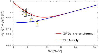
(a) $Q^{2}=1.6-1.9$ GeV²

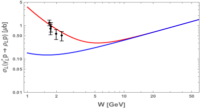
(b) $Q^{2}=1.9-2.2$ GeV²

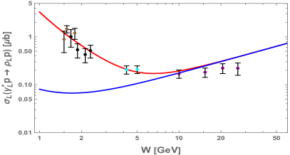
(c) $Q^{2}=2.2-2.5$ GeV²

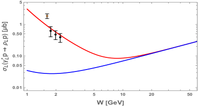
(d) $Q^{2}=2.5-2.8$ GeV²

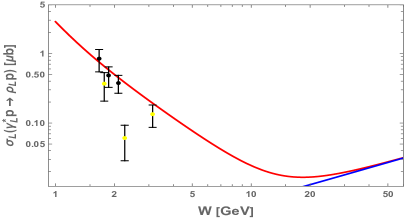
(e) $Q^{2}=2.8-3.1$ GeV²

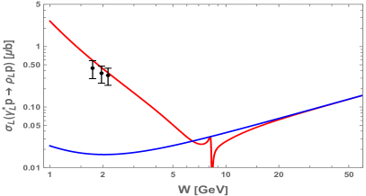
(f) $Q^{2}=3.1-3.6$ GeV²

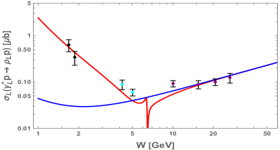
(g) $Q^{2}=3.6-4.1$ GeV²

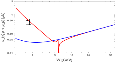
(h) $Q^{2}=4.1-4.6$ GeV²

(i) $Q^{2}=4.6-5.1$ GeV²

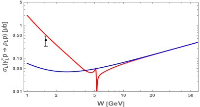
(j) $Q^{2}=5.1-5.6$ GeV²

Figure 7: Longitudinal cross section for the electroproduction of neutral rho mesons versus $W=\sqrt{s}$ in GeV.

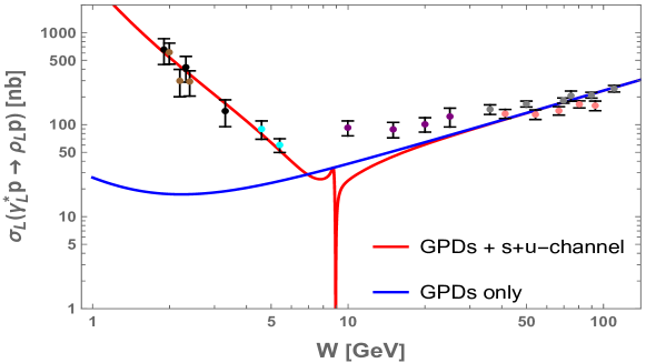
(a)

Figure 8: Longitudinal cross section for the electroproduction of neutral rho mesons versus $W=\sqrt{s}$ in GeV, for $Q^{2}=4$ GeV². The solid-blue curves are with the evolved up and down singlet quark, and gluon GPDs. The red curves are the sum of the s-channel background, and the evolved up and down singlet quark, and gluon GPD contribution at amplitude level (i.e., (IV.85)). Note that here we have also re-scaled our total cross section by an overall factor of $10^{3}$ since the unit of the cross section here is in nb. The brown data points are from 4.2 GeV CLAS Hadjidakis et al. (2005). The black data points are from 5.754 GeV CLAS Morrow et al. (2009). The cyan data points are from HERMES Airapetian et al. (2000). The purple data points are from E665 Adams et al. (1997). The grey data points are from ZEUS Breitweg et al. (1999). The pink data points are from H1 Adloff et al. (2000a).

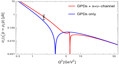
(a) $x_{B}=0.16-0.22$

(b) $x_{B}=0.22-0.28$

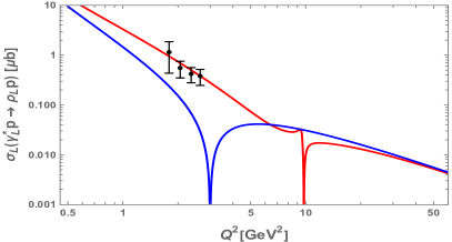
(c) $x_{B}=0.28-0.34$

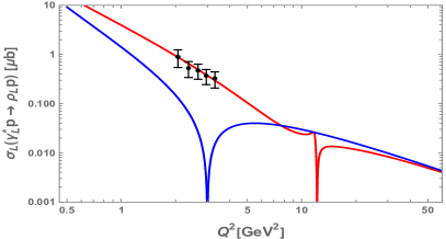
(d) $x_{B}=0.34-0.4$

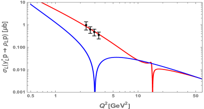
(e) $x_{B}=0.40-0.46$

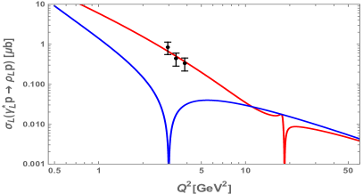
(f) $x_{B}=0.46-0.52$

(g) $x_{B}=0.52-0.58$

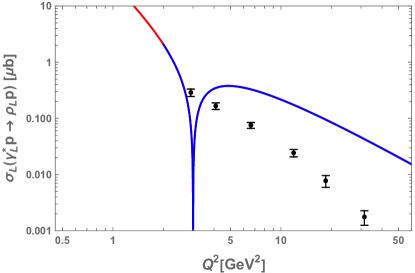
(h) $W=\sqrt{s}=75$ GeV

Figure 9: Longitudinal cross section for the electroproduction of neutral rho mesons versus $Q^{2}$ in GeV², for different values of Bjorken $x_{B}$ as indicated in the alphabet label of each subfigure, except for the last subfigure where the value of $W$ is added. The solid-blue curves are with the evolved up and down singlet quark, and gluon GPD contributions. The red curves are the sum of the s-channel background, and the evolved up and down singlet quark, and gluon GPD contributions at amplitude level. The black data points are from 5.754 GeV CLAS Morrow et al. (2009).

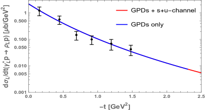
(a) $Q^{2}=0-1.9$ GeV², $\mathbf{x_{B}}=\mathbf{0.16-0.22}$

(b) $Q^{2}=2.2-2.5$ GeV², $\mathbf{x_{B}}=\mathbf{0.22-0.28}$

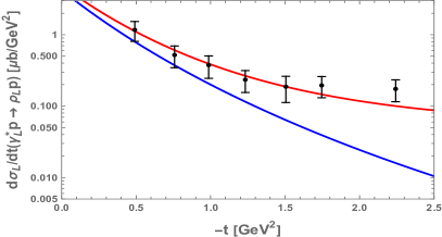
(c) $Q^{2}=1.9-2.2$ GeV², $\mathbf{x_{B}}=\mathbf{0.34-0.40}$

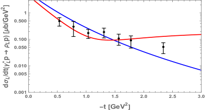
(d) $Q^{2}=3.1-3.6$ GeV², $\mathbf{x_{B}}=\mathbf{0.40-0.46}$

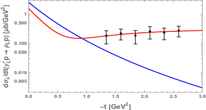
(e) $Q^{2}=4.1-4.6$ GeV², $\mathbf{x_{B}}=\mathbf{0.58-0.64}$

Figure 10: Longitudinal differential cross section for the electroproduction of neutral rho mesons versus $-t$ in GeV², for different values of $Q^{2}$ and $x_{B}$ as indicated in the alphabet label of each subfigure. The solid-blue curves are with the evolved up and down singlet quark, and gluon GPD contributions. The red curves are the sum of the s-channel, and the evolved up and down singlet quark, and gluon GPDs at amplitude level (i.e., (IV.5)). Note that with increasing $x_{B}\geq 0.34$, that is, in (c) to (e), the contribution from the $s+u$-channel starts to control the $t$ dependence in the large $t$ regime. The black data points are from 5.754 GeV CLAS Morrow et al. (2009), see Fig. 26 in Morrow et al. (2009).

IV.7 Comparison to experiment for $\rho^{0}$

Here, we present the comparison of our results with experimental measurements. In Table 1, we provide the values of various parameters such as $\lambda$, $\tau$, $\tilde{\kappa}_{T,S}$, and $\tilde{\kappa}_{N,V}$, which have been obtained previously by constraining the electromagnetic and gravitational form factors and the holographic $J/\psi$ photoproduction in the high energy limit Mamo and Zahed (2021b). These parameters are fixed and predetermined for the GPDs under consideration here.

However, the normalization constants $\mathcal{N}_{t,s}$ have been determined empirically by fitting to the analyzed cross sections shown in Figs. 7 - 10, as summarized in Table 1. It is important to note that the same normalization constants $\mathcal{N}_{t}=1.687$ and $\mathcal{N}_{s}=-131.503$ have been used for all the total cross section figures shown in Figs. 7 - 9.

However, different normalization constants $\mathcal{N}_{t,s}$ have been used for each bin in the differential cross section vs. $-t$ figures shown in Figs. 10a - 10e. This is because the kinematic factors of order $\mathcal{O}(-t/Q^{2})$ have been ignored for both the $s+u$-channel and GPD contributions, which do not affect the total cross sections (shown in Figs. 7 - 9) computed at $-t=0$ using the optical theorem (IV.85).

Furthermore, the values of the physical parameters $m_{N}=0.94~{}\text{GeV}$, $m_{\rho^{0,+}}=0.775~{}\text{GeV}$, and $f^{\prime}_{\rho^{0,+}}=f_{\rho^{0,+}}=0.216~{}\text{GeV}$ have been used throughout the analysis. In Figs. 7, the solid-blue curves are using the evolved singlet quark (up and down) and gluon GPDs,the red curves are the sum of the s-channel background, and the evolved singlet quark plus gluon GPDs (i.e., (IV.85)), the brown data points are from 4.2 GeV CLAS Hadjidakis et al. (2005), the yellow data points are from CORNELL Cassel et al. (1981), the cyan data points are from HERMES Airapetian et al. (2000), the purple data points are from E665 Adams et al. (1997), the black data points are from 5.754 GeV CLAS Morrow et al. (2009).

V Electroproduction of longitudinal $\phi$ meson with evolved gluon GPD: a comparison to experiment

The electroproduction of $\phi$ meson with the evolved gluon GPD is similar to the gluon contribution to $\rho^{0}$ meson (IV.57), and is given by

$${\cal A}^{LL(gluon)}_{\gamma^{*}p\rightarrow\phi p}(s,t,Q,\epsilon_{L},\epsilon_{L}^{\prime}) \propto \widehat{\widehat{\mathbb{F}}}^{g}_{j_{0g}}(\xi,t;\mu^{2})\times f_{V}^{\prime}\,\alpha_{s}(\mu)\,{1\over{Q}}\,\frac{1}{2\sqrt{2}m_{N}}\,\bar{u}(p_{2})u(p_{1})$$ (V.86)

$$\times \left[\frac{(\sqrt{\lambda}/\pi)}{\xi^{2-2/\sqrt{\lambda}}}+\frac{i}{\xi^{2-2/\sqrt{\lambda}}}\right]$$

$$\propto {\cal A}^{gluon}_{\phi}(s,t,Q)\times\frac{1}{2\sqrt{2}m_{N}}\,\bar{u}(p_{2})u(p_{1})\,,$$

with $j_{0g}=2-2/\sqrt{\lambda}$, $\tilde{\tau}=\text{log}(1/\xi)$, and $f_{V}^{\prime}\approx f_{V}$. In terms of (V.86), the total longitudinal differential cross section for electroproduction of $\phi$ meson reads

$$\frac{d\sigma_{L}(\phi)}{dt} = \frac{1}{16\pi s^{2}}\times\frac{1}{2}\sum_{\rm spin}\Big{|}\mathcal{N}_{t}\times\mathcal{A}_{\gamma^{*}p\rightarrow\phi p}^{LL(gluon)}\Big{|}^{2}$$ (V.87)

$$= \frac{1}{16\pi s^{2}}\times\frac{1}{2}\ \Big{|}\mathcal{N}_{t}\times\mathcal{A}_{\phi}^{gluon}\Big{|}^{2}\,,$$

where the total amplitude $\mathcal{A}_{\phi}^{gluon}$ is defined in (V.86). We also compute the total cross section using the optical theorem as

$$\sigma_{L}(\phi)=\left(\frac{16\pi\,\frac{d\sigma_{L}(\phi)}{dt}}{1+\rho}\right)^{1/2}_{t=0}\,,$$ (V.88)

where $\rho$ is the ratio of the real and imaginary part of the total amplitude. We have compared our total cross section (V.88) to experimental data in Fig. 11 and 12. Note that these relations carry to heavier mesons $J/\Psi$ and $\Upsilon$ with slight changes.

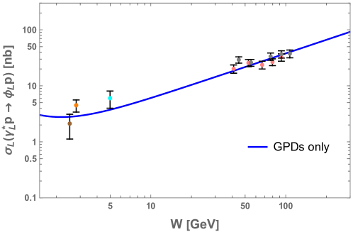
(a)

Figure 11: Longitudinal cross section for the electroproduction of phi mesons versus $W=\sqrt{s}$ in GeV, for $Q^{2}=3.8$ GeV² (solid-blue curves) in (V.88) with $\mathcal{N}_{t}=0.2$. The solid-blue curves are only with the evolved gluon GPD. The orange data point is from CLAS 2008 Santoro et al. (2008). The brown data point is from CLAS 2001 Lukashin et al. (2001). The cyan data point is from HERMES 2000. The grey data points are from ZEUS Chekanov et al. (2005). The pink data points are from H1 Adloff et al. (2000b).

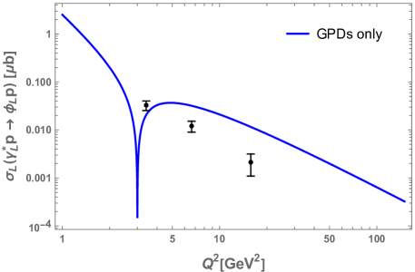
(a)

Figure 12: Longitudinal cross section for the electroproduction of phi mesons versus $Q^{2}$ in GeV², for $W=\sqrt{s}=75$ GeV (solid-blue curve) in (V.88) with $\mathcal{N}_{t}=0.2$. The solid-blue curve is only with the evolved gluon GPD. The black data points are from H1, ZEUS Aaron et al. (2010).

V.1 Comparison to experiment for $\phi$

In Table 1, we present the parameters for the AdS construction with a soft wall: $\lambda=11.243$, $\tau=3$, $\tilde{\kappa}_{T,S}=0.388~{}\text{GeV}$, and $\tilde{\kappa}_{N,V}=0.402~{}\text{GeV}$, as well as the normalization constants $\mathcal{N}_{t}=0.200$, and $\mathcal{N}_{s}=0$. We then illustrate the longitudinal cross section for the electroproduction of phi mesons ($\mathcal{N}_{t}=0.200$ in Eq. (V.88)) as a function of $W=\sqrt{s}$ and $Q^{2}$ in Fig. 11 and Fig. 12, respectively. The values of the physical parameters used are $m_{N}=0.94~{}\text{GeV}$, $m_{\phi}=1.019~{}\text{GeV}$, and $f^{\prime}_{\phi}=f_{\phi}=0.233~{}\text{GeV}$.

It is important to note that the solid-blue curve represents the evolved gluon GPD only, as the strange singlet quark GPD has been set to zero. Additionally, we assume the phi meson’s coupling to the proton ($g_{\phi pp}=0$) to be zero, effectively setting the s-channel background contribution to zero. Experimental data points are included from various sources: CLAS 2008 (orange) Santoro et al. (2008), CLAS 2001 (brown) Lukashin et al. (2001), HERMES 2000 (cyan) Kroll (2015), ZEUS (grey) Chekanov et al. (2005), H1 (pink) Adloff et al. (2000b), and H1, ZEUS (black) Aaron et al. (2010). Figures 5 and 7 from Kroll (2015) and Favart et al. (2016), respectively, also display these data points.

VI Electroproduction of longitudinal $\rho^{+}$ meson with evolved valence quark GPDs: a comparison to experiment

The electroproduction of longitudinal charged rho meson ($\rho^{+}$) in terms of quark DAs and quark GPDs is given by (see Eq.219 with Eq.222 and Eq.223 in Goeke et al. (2001))

$${\cal A}^{LL}_{\gamma^{*}p\rightarrow\rho^{+}n}(s,t,Q,\epsilon_{L},\epsilon_{L}^{\prime})=$$

$$-e\times{C_{F}\over N_{c}}\times{1\over 2}\times(4\pi\alpha_{s}(\mu^{2}))\times{1\over{Q}}\times\left[\,\int_{0}^{1}dz{{\Phi_{\rho^{+}}(z)}\over z}\right]\times\frac{1}{p^{+}}\left\{A_{\rho^{+}\,n}\,h^{+}\,+\,B_{\rho^{+}\,n}\,e^{+}\right\}\,,$$ (VI.89)

where $\Phi_{\rho^{+}}(z)$ is the charged rho meson ($\rho^{+}$) distribution amplitude (DA), and

$$A_{\rho^{+}\,n}\, = \,\int_{-1}^{1}dx\;{\left(H^{u}(x,\eta,t;\mu^{2})\,-\,H^{d}(x,\eta,t;\mu^{2})\right)}\;\left\{{{Q_{u}}\over{\xi-x-i\epsilon}}-{{Q_{d}}\over{\xi+x-i\epsilon}}\right\}$$

$$B_{\rho^{+}\,n}\, = \,\int_{-1}^{1}dx\;{\left(E^{u}(x,\eta,t;\mu^{2})\,-\,E^{d}(x,\eta,t;\mu^{2})\right)}\;\left\{{{Q_{u}}\over{\xi-x-i\epsilon}}-{{Q_{d}}\over{\xi+x-i\epsilon}}\right\}\,.$$ (VI.90)

Using $C_{F}=\frac{N_{c}^{2}-1}{2N_{c}}$, and $Q_{u}=+2/3\,(Q_{d}=-1/3)$, we can rewrite (VI-VI) as

$${\cal A}^{LL}_{\gamma^{*}p\rightarrow\rho^{+}n}(s,t,Q,\epsilon_{L},\epsilon_{L}^{\prime}) \,=\, -e\times{1\over 2}\times\left(1-\frac{1}{N_{c}^{2}}\right)\times 4\pi\times\alpha_{s}(\mu^{2})$$ (VI.91)

$$\times {1\over{Q}}\times\left[\,\int_{0}^{1}dz{{\Phi_{\rho^{+}}(z)}\over z}\right]\times\frac{1}{p^{+}}\times u(p_{2})\gamma^{+}u(p_{1})$$

$$\times \Bigg{[}\int_{0}^{1}dx\;{\left(H_{valence}^{u}(x,\eta,t;\mu^{2})\,-\,H_{valence}^{d}(x,\eta,t;\mu^{2})\right)}\;\left\{\frac{\xi}{2x}\times\frac{2x}{\xi^{2}-x^{2}}\right\}$$

$$+ \int_{0}^{1}dx\;{\left(H_{singlet}^{u}(x,\eta,t;\mu^{2})\,-\,H_{singlet}^{d}(x,\eta,t;\mu^{2})\right)}\;\left\{\frac{1}{6}\times\frac{2x}{\xi^{2}-x^{2}}\right\}$$

$$+ i\pi\times Q_{u}\left(H^{u}(\xi,\eta,t;\mu^{2})\,-\,H^{d}(\xi,\eta,t;\mu^{2})\right)$$

$$-i \pi\times Q_{d}\left(H^{u}(-\xi,\eta,t;\mu^{2})\,-\,H^{d}(-\xi,\eta,t;\mu^{2})\right)\Bigg{]}\,,$$

where we have defined $H_{valence}^{q}(x,\eta,t;\mu^{2})=H^{q}(x,\eta,t;\mu^{2})+H^{q}(-x,\eta,t;\mu^{2})$, $H_{singlet}^{q}(x,\eta,t;\mu^{2})=H^{q}(x,\eta,t;\mu^{2})-H^{q}(-x,\eta,t;\mu^{2})$, and we have ignored the Pauli contribution for $-t\ll 4m_{N}^{2}$.

Ignoring the singlet quark GPDs contribution in (VI.91) by assuming $H^{u}_{singlet}=H^{d}_{singlet}$, the longitudinal electroproduction of $\rho^{+}$ meson with only evolved valence quark GPDs is given by

$${\cal A}^{LL(valence)}_{\gamma^{*}p\rightarrow\rho^{+}n}(s,t,Q,\epsilon_{L},\epsilon_{L}^{\prime})$$ (VI.92)

$$= -e\times{1\over 2}\times{1\over 2}\times\left(1-\frac{1}{N_{c}^{2}}\right)\times 4\pi\alpha_{s}(\mu)\times{1\over{Q}}\times\left[\,\int_{0}^{1}dz{{\Phi_{\rho^{+}}(z)}\over z}\right]\times\frac{1}{2m_{N}}\times\bar{u}(p_{2})u(p_{1})$$

$$\times \Bigg{[}\int_{0}^{1}dx\,\,\frac{\xi}{2x}\times\frac{2x}{\xi^{2}-x^{2}}\times\left(H_{valence}^{u}(x,\eta,t;\mu^{2})\,-\,H_{valence}^{d}(x,\eta,t;\mu^{2})\right)$$

$$+ i\pi\times Q_{u}\left(H^{u}(\xi,\eta,t;\mu^{2})\,-\,H^{d}(\xi,\eta,t;\mu^{2})\right)-i\pi\times Q_{d}\left(H^{u}(-\xi,\eta,t;\mu^{2})\,-\,H^{d}(-\xi,\eta,t;\mu^{2})\right)\Bigg{]}\,,$$

$$\,=\, -e\times{1\over 2}\times{1\over 2}\times\left(1-\frac{1}{N_{c}^{2}}\right)\times 4\pi\alpha_{s}(\mu)\times{1\over{Q}}\times\left[\,\int_{0}^{1}dz{{\Phi_{\rho^{+}}(z)}\over z}\right]\times\frac{1}{2m_{N}}\times\bar{u}(p_{2})u(p_{1})$$

$$\times \Bigg{[}\frac{1}{\xi}\times\sum_{j=1}^{\infty}\frac{1}{\eta^{j-1}}\times\frac{1}{N_{j-1}(\frac{3}{2})}\times\left[\int_{0}^{\eta}\frac{dx}{\eta}\,\frac{\left(1-\frac{x^{2}}{\eta^{2}}\right)}{1-\frac{x^{2}}{\xi^{2}}}\times C_{j-1}^{3/2}\left(\frac{x}{\eta}\right)\right]\times\left(\mathbb{F}^{u}_{j(valence)}(\eta,t;\mu^{2})\,-\,\mathbb{F}^{d}_{j(valence)}(\eta,t;\mu^{2})\right)$$

$$+ i\pi\times Q_{u}\left(H^{u}(\xi,\eta,t;\mu^{2})\,-\,H^{d}(\xi,\eta,t;\mu^{2})\right)-i\pi\times Q_{d}\left(H^{u}(-\xi,\eta,t;\mu^{2})\,-\,H^{d}(-\xi,\eta,t;\mu^{2})\right)\Bigg{]}\,,$$

$$\,\approx\, -e\times{1\over 2}\times\left(1-\frac{1}{N_{c}^{2}}\right)\times 4\pi\alpha_{s}(\mu)\times{1\over{Q}}\times\left[\,\int_{0}^{1}dz{{\Phi_{\rho^{+}}(z)}\over z}\right]\times\frac{1}{2m_{N}}\times\bar{u}(p_{2})u(p_{1})$$

$$\times \sum_{j=1}^{\infty}\frac{1}{\xi^{j}}\times\frac{1}{N_{j-1}(\frac{3}{2})}\times\left[\int_{0}^{\xi}\frac{dx}{\xi}\,C_{j-1}^{3/2}\left(\frac{x}{\xi}\right)\right]\times\left(\mathbb{F}^{u}_{j(valence)}(\eta\sim\xi,t;\mu^{2})\,-\,\mathbb{F}^{d}_{j(valence)}(\eta\sim\xi,t;\mu^{2})\right)\,,$$

with odd $j=1,3,...$, and in the last line we have used $\eta\sim\xi$. Again, the $i\pi H^{u,d}$ contributions vanish for $\xi=\pm\eta$. We can also rewrite (VI.92) more compactly as

$${\cal A}^{LL(valence)}_{\gamma^{*}p\rightarrow\rho^{+}n}(s,t,Q,\epsilon_{L},\epsilon_{L}^{\prime})\approx-e\times f_{V}^{+}\times\alpha_{s}(\mu)\times{1\over{Q}}$$

$$\times\sum_{j=1}^{\infty}\frac{1}{\xi^{j}}\times\mathcal{N}_{q(valence)}(j)\times\left(\mathbb{F}^{u}_{j(valence)}(\xi,t;\mu^{2})\,-\,\mathbb{F}^{d}_{j(valence)}(\xi,t;\mu^{2})\right)\times\frac{1}{2m_{N}}\times\bar{u}(p_{2})u(p_{1})\,,$$

where we have defined

$$\mathcal{N}_{q(valence)}(j) \equiv {1\over 2}\times\left(1-\frac{1}{N_{c}^{2}}\right)\times 4\pi\times\frac{1}{N_{j-1}(\frac{3}{2})}\times I_{q(valence)}(j)\,,$$ (VI.94)

and the integrals (with $\tilde{x}=x/\xi$)

$$f_{V}^{+}=\int_{0}^{1}dz{{\Phi_{\rho^{+}}(z)}\over z}\,,\qquad\qquad I_{q(valence)}(j)=\left[\int_{0}^{1}d\tilde{x}\,C_{j-1}^{3/2}\left(\tilde{x}\right)\right]\,,$$ (VI.95)

VI.1 Final amplitude for $\rho^{+}$

Figure 13: Illustration of the integration contour $\mathbb{C}$ in the complex j-plane used for computing the contour integral (G), with a branch cut displayed for $\text{Re(j)}\leq j_{0q}=1-1/\sqrt{\lambda}$.

The resummation by j-contour for the valence quark GPDs contribution (VI) is similar to the resummation for the singlet quark and gluon GPDs (albeit using a different integration contour shown in Fig. 13), and the detailed derivation is given in Appendix G. Here we only provide the final answer.

After the resummation of (VI) using the contour integral (G) with the integration contour $\mathbb{C}$ in the complex j-plane, shown in Fig. 13, and using the result for $\text{Re}\left[{\cal A}^{LL(valence)}\right]$ given in (G) and $\text{Im}\left[{\cal A}^{LL(valence)}\right]$ given in (G.247), the full complex amplitude with the evolved valence quark GPDs is given by

$${\cal A}^{LL(valence)}_{\gamma^{*}p\rightarrow\rho^{+}n}(s,t,Q,\epsilon_{L},\epsilon_{L}^{\prime})$$

$$\propto\Bigg{(}\widehat{\mathbb{F}}^{u}_{j_{0q}(valence)}(\xi,t;\mu^{2})-\widehat{\mathbb{F}}^{d}_{j_{0q}(valence)}(\xi,t;\mu^{2})\Bigg{)}\times\Bigg{[}(\sqrt{\lambda}/4\pi)^{1/2}\times\frac{1}{\xi}\times(\sqrt{\lambda}/2\pi)\times e^{-\tilde{\tau}/\sqrt{\lambda}}\times\frac{e^{-\sqrt{\lambda}/4\tilde{\tau}}}{\tilde{\tau}^{3/2}}$$

$$+i\times\frac{1}{\xi^{j_{0q}}}\times(\sqrt{\lambda}/4\pi)^{1/2}\times\frac{e^{-\sqrt{\lambda}/4\tilde{\tau}}}{\tilde{\tau}^{3/2}}\Bigg{]}\times\mathcal{N}_{q(valence)}(j_{0q})\times(-1)\times e\,f_{V}^{+}\,\alpha_{s}(\mu)\,{1\over{Q}}\,\frac{1}{2m_{N}}\,\bar{u}(p_{2})u(p_{1})\,,$$

$$\propto\Bigg{(}\widehat{\widehat{\mathbb{F}}}^{u}_{j_{0q}(valence)}(\xi,t;\mu^{2})-\widehat{\widehat{\mathbb{F}}}^{d}_{j_{0q}(valence)}(\xi,t;\mu^{2})\Bigg{)}\times(-1)\times f_{V}^{+}\,\alpha_{s}(\mu)\,{1\over{Q}}\,\frac{1}{2m_{N}}\,\bar{u}(p_{2})u(p_{1})$$

$$\times\left[\frac{(\sqrt{\lambda}/2\pi)}{\xi^{1-1/\sqrt{\lambda}}}+\frac{i}{\xi^{1-1/\sqrt{\lambda}}}\right]\,,$$

$$\propto{\cal A}^{valence}_{\rho^{+}}(s,t,Q)\times\frac{1}{2\sqrt{2}m_{N}}\,\bar{u}(p_{2})u(p_{1})\,,$$ (VI.96)

where we have absorbed $e\times\mathcal{N}_{q(valence)}(j_{0q})\times(\sqrt{\lambda}/4\pi)^{1/2}\times\frac{e^{-\sqrt{\lambda}/4\tilde{\tau}}}{\tilde{\tau}^{3/2}}$ into the normalization constant as it varies slowly with $s$. We have also defined the normalized and flavor separated quark conformal moments as

$$\widehat{\widehat{\mathbb{F}}}^{u+d}_{j(valence)}(\xi,t;\mu^{2}) = 0.151\times\frac{\widehat{\mathbb{F}}^{q}_{j(valence)}(\xi,t;\mu^{2})}{\widehat{\mathbb{F}}^{q}_{j=3(valence)}(\xi=0,t=0;\mu^{2}=4~{}\text{GeV}^{2})}\,,$$

$$\widehat{\widehat{\mathbb{F}}}^{u-d}_{j(valence)}(\xi,t;\mu^{2}) = 0.070\times\frac{\widehat{\mathbb{F}}^{q}_{j(valence)}(\xi,t;\mu^{2})}{\widehat{\mathbb{F}}^{q}_{j=3(valence)}(\xi=0,t=0;\mu^{2}=4~{}\text{GeV}^{2})}\,,$$

$$\widehat{\widehat{\mathbb{F}}}^{u}_{j(valence)}(\xi,t;\mu^{2}) = \frac{1}{2}\times\left(\widehat{\widehat{\mathbb{F}}}^{u+d}_{j(valence)}(\xi,t;\mu^{2})+\widehat{\widehat{\mathbb{F}}}^{u-d}_{j(valence)}(\xi,t;\mu^{2})\right)\,,$$

$$\widehat{\widehat{\mathbb{F}}}^{d}_{j(valence)}(\xi,t;\mu^{2}) = \frac{1}{2}\times\left(\widehat{\widehat{\mathbb{F}}}^{u+d}_{j(valence)}(\xi,t;\mu^{2})-\widehat{\widehat{\mathbb{F}}}^{u-d}_{j(valence)}(\xi,t;\mu^{2})\right)\,,$$ (VI.97)

where the normalization coefficients are fixed using the lattice data in Hagler et al. (2008), and $\widehat{\mathbb{F}}^{q}_{j(valence)}(\xi,t;\mu^{2})=\Gamma(\Delta_{q}(j)-2)\times\mathbb{F}^{q}_{j(valence)}(\xi,t;\mu^{2})$ is given in (III.19). Note that we have used the average value of $A_{3}^{u+d}(-t=0)=\widehat{\widehat{\mathbb{F}}}^{u+d}_{j=3(valence)}(\xi=0,t=0;\mu^{2}=4~{}\text{GeV}^{2})=0.151$ from Table XV and Table XVI of Hagler et al. (2008). We have also used the value of $A_{3}^{u-d}(-t=0)=\widehat{\widehat{\mathbb{F}}}^{u-d}_{j=3(valence)}(\xi=0,t=0;\mu^{2}=4~{}\text{GeV}^{2}=0.070$ from Table IX of Hagler et al. (2008).

VI.2 Differential and total cross sections for $\rho^{+}$

Finally, using the valence quark GPDs contribution (VI.1), we have the total longitudinal differential cross section for electroproduction of $\rho^{+}$ meson

$$\frac{d\sigma_{L}(\rho^{+})}{dt} = \frac{1}{16\pi s^{2}}\times\frac{1}{2}\sum_{\rm spin}\Big{|}\mathcal{N}_{t}\times\mathcal{A}_{\gamma^{*}p\rightarrow\rho^{+}n}^{LL(valence)}\Big{|}^{2}$$ (VI.98)

$$= \frac{1}{16\pi s^{2}}\times\frac{1}{2}\Big{|}\mathcal{N}_{t}\times\mathcal{A}_{\rho^{+}}^{valence}\Big{|}^{2}\,.$$

We also calculate the total cross section using the optical theorem as

$$\sigma_{L}(\rho^{+})=\left(\frac{16\pi\,\frac{d\sigma_{L}(\rho^{+})}{dt}}{1+\rho}\right)^{1/2}_{t=0}\,,$$ (VI.99)

where $\rho$ is the ratio of the real and imaginary part of our total complex amplitude. We have compared our total cross section (VI.99) to the experimental data in Fig. 14. We fix the value of the normalization parameter $\mathcal{N}_{t}$ by the charged rho meson data as detailed in the next subsection below.

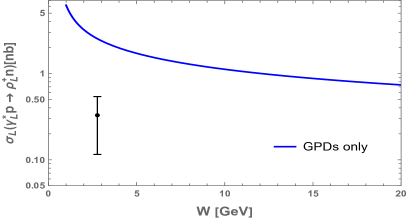
(a) $Q^{2}=1-1.5$ GeV²

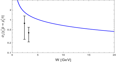
(b) $Q^{2}=1.5-2.0$ GeV²

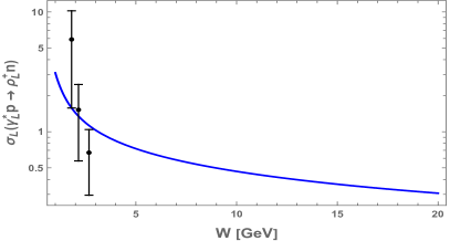
(c) $Q^{2}=2.0-2.5$ GeV²

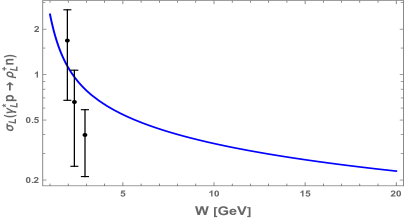
(d) $Q^{2}=2.5-3.0$

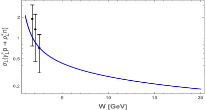
(e) $Q^{2}=3.0-3.5$ GeV²

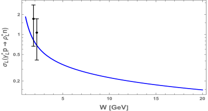
(f) $Q^{2}=3.5-4.0$

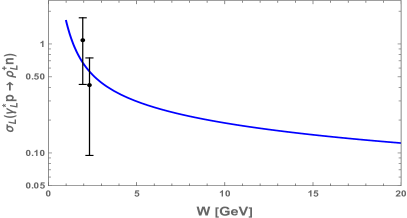
(g) $Q^{2}=4.0-4.5$ GeV²

Figure 14: Longitudinal cross section for the electroproduction of charged rho mesons ($\rho^{+}$) versus $W=\sqrt{s}$ in GeV.The blue curve is with the evolved valence up and down quark GPDs (i.e., (VI.99). The black data points are from 5.776 GeV CLAS Fradi (2011).

VI.3 Comparison to experiment for $\rho^{+}$

In this section, we present our result for the electroproduction of charged rho mesons ($\rho^{+}$) and its comparison to experimental data. First, we list the parameters used in our AdS construction with a soft wall, namely $\lambda=11.243$, $\tau=3$, $\tilde{\kappa}_{T,S}=0.388~{}\text{GeV}$, $\tilde{\kappa}_{N,V}=0.402~{}\text{GeV}$, and the normalization constants $\mathcal{N}_{t}=724.513$ and $\mathcal{N}_{s}=0$, which are given in Table 1.

Next, we show the longitudinal cross section for the electroproduction of $\rho^{+}$ mesons versus $W=\sqrt{s}$ in GeV in Fig. 14. In these figures, we have used the evolved valence up and down quark GPDs (i.e., (VI.99)) with $\mathcal{N}_{t}=724.513$. We have also used the values of the physical parameters $m_{N}=0.94~{}\text{GeV}$, $m_{\rho^{0,+}}=0.775~{}\text{GeV}$, and $f^{\prime}_{\rho^{0,+}}=f_{\rho^{0,+}}=0.216~{}\text{GeV}$. It is important to note that we have assumed that the coupling of the $\rho^{+}$ meson to the proton and neutron ($g_{\rho^{+}pn}$) is zero and we have set the s-channel contribution to zero, that is, $\mathcal{N}_{s}=0$.

In the comparison of our results with experimental data, in Fig. 14, the black data points are from the 5.776 GeV CLAS experiment Fradi (2011) (see Fig.4 of Fradi (2011)).

VII Summary and Conclusion

In this paper, we have presented a framework for constructing General Parton Distributions (GPDs) at low-x and finite skewness using holographic QCD in the double limit of large $N_{c}$ and strong gauge coupling. We have first constructed holographic amplitudes for exclusive electroproduction processes, dominated by bulk spin-j gravitons and vector or axial meson exchanges in AdS, which are dual to Pomerons and Reggeons in QCD, respectively. By comparing the holographic exclusive amplitudes with the corresponding exclusive amplitudes in QCD, which are based on factorization theorems, we have extracted the spin-j conformal moments of GPDs and constructed the GPDs.

Using the holographically fixed conformal moments of GPDs at the initial or low renormalization scale $\mu\sim\mu_{0}\sim 1.8$ GeV, we have used one-loop pQCD evolution equations to obtain their counterparts at a higher renormalization scale $\mu>\mu_{0}$, which enhances the perturbative partonic content at low-x in addition to the nonperturbative one captured by the holographic construction at the low renormalization scale.

We have used our evolved GPDs to specifically determine the exclusive longitudinal electroproduction of neutral rho ($\rho^{0}$), phi ($\phi$), and charged rho ($\rho^{+}$) mesons, using the factorization theorems in QCD, and compare them to the existing data from CLAS, HERMES, and H1 experiments. Specifically, in the data analysis of the longitudinal electroproduction of $\rho^{0}$, we have found that the holographic GPDs (similar to previous GPD models) alone cannot explain the low $\sqrt{s}$ data, and we have accounted for the non-perturbative physics coming from the s-channel. We have successfully determined such non-perturbative contribution in the s-channel using holographic QCD and found that its contribution at low $\sqrt{s}$ is in good agreement with the experimental data. We expect the holographic s-channel contribution to play a key role in the future experimental extraction of GPDs at JLab and future EIC.

Our extracted quark and gluon GPDs for fixed skewness $\eta$ provide explicit and detailed dependence on the kinematical variables $t$ and $\eta$, with their moments satisfying all the polynomiality conditions in $\eta$. They should prove useful for extracting the GPDs using global data analysis and carry detailed tomographic information about the partonic distributions inside a nucleon after Fourier transforming to coordinate space with respect to $t$.

Additionally, our framework can be extended to longitudinal heavier vector mesons such as $J/\Psi$ and $\Upsilon$, and yields detailed predictions for exclusive processes such as the electroproduction of photons in DVCS or the longitudinal electroproduction of single and double axial mesons.

In conclusion, this paper provides a powerful framework for constructing GPDs at low-x and finite skewness using holographic QCD in the large $N_{c}$ limit. We have demonstrated the potential of this approach for analyzing exclusive electroproduction processes and provided useful results for future experimental studies and global data analyses.

Acknowledgments

K.M. is supported by the U.S. Department of Energy, Office of Science, Office of Nuclear Physics, contract no. DE-AC02-06CH11357, and an LDRD initiative at Argonne National Laboratory under Project No. 2020-0020. I.Z. is supported by the Office of Science, U.S. Department of Energy under Contract No. DE-FG-88ER40388.

Appendix A Notations

Here, we summarize the key notations used for the GPDs and their conformal (Gegenbauer) moments:

$$H^{q}(x) \equiv\text{quark GPDs}\,,$$

$$\widetilde{H}^{q}(x) \equiv\text{axial quark GPDs}\,,$$

$$H^{g}(x) \equiv\text{gluon GPDs}\,,$$

$$H_{\text{valence}}^{q}(x) \equiv\text{valence quark GPDs, which are }H^{q}(x)+H^{q}(-x)\,,$$

$$H_{\text{singlet}}^{q}(x) \equiv\text{singlet quark GPDs, which are }H^{q}(x)-H^{q}(-x)\,,$$

$$\widetilde{H}_{\text{valence}}^{q}(x) \equiv\text{valence axial quark GPDs, which are }\widetilde{H}^{q}(x)-\widetilde{H}^{q}(-x)\,,$$

$$\widetilde{H}_{\text{singlet}}^{q}(x) \equiv\text{singlet axial quark GPDs, which are }\widetilde{H}^{q}(x)+\widetilde{H}^{q}(-x)\,,$$

$$\mathbb{F}^{q}_{j(\text{valence})} \equiv\text{conformal (Gegenbauer) moments of valence quark GPDs}\,,$$

$$\mathbb{F}^{q}_{j(\text{singlet})} \equiv\text{conformal (Gegenbauer) moments of singlet quark GPDs}\,,$$

$$\widetilde{\mathbb{F}}^{q}_{j(\text{valence})} \equiv\text{conformal (Gegenbauer) moments of valence axial quark GPDs}\,,$$

$$\widetilde{\mathbb{F}}^{q}_{j(\text{singlet})} \equiv\text{conformal (Gegenbauer) moments of singlet axial quark GPDs}\,,$$

$$\mathbb{F}^{g}_{j} \equiv\text{conformal (Gegenbauer) moments of gluon GPD}.$$

Appendix B Kinematics

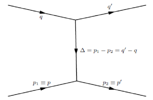
Figure 15: Illustration of the kinematic variables defined in (B.100) - (B.106).

Here, we summarize the pertinent kinematics for the GPDs, see Fig. 15. Following Belitsky and Radyushkin (2005), we define

$$\tilde{q}=\frac{1}{2}(q+q^{\prime})\,,\qquad p=\frac{1}{2}(p_{1}+p_{2})\,,\qquad\Delta=p_{1}-p_{2}=q^{\prime}-q\,.$$ (B.100)

$$\tilde{q}^{2}=-\tilde{Q}^{2}\,,\qquad\xi=\frac{\tilde{Q}^{2}}{2p\cdot\tilde{q}}\,,\qquad\eta=\frac{\Delta\cdot\tilde{q}}{2p\cdot\tilde{q}}\,.$$ (B.101)

$$Q^{2}=-q^{2}\,,\qquad Q^{\prime 2}=-q^{\prime 2}\,,\qquad x_{\rm B}=\frac{{Q}^{2}}{2p_{1}\cdot q}\,,$$ (B.102)

$$\tilde{Q}^{2}=\frac{1}{2}\left(Q^{2}+Q^{\prime 2}+\frac{\Delta^{2}}{2}\right)\,,$$ (B.103)

$$\xi=\frac{Q^{2}+Q^{\prime 2}+\Delta^{2}/2}{2Q^{2}/x_{\rm B}-Q^{2}+Q^{\prime 2}+\Delta^{2}}\,,\qquad\eta=\frac{Q^{2}-Q^{\prime 2}}{2Q^{2}/x_{\rm B}-Q^{2}+Q^{\prime 2}+\Delta^{2}}\,,$$ (B.104)

$$Q^{\prime 2}=\left(1-\frac{\eta}{\xi}\right)\tilde{Q}^{2}-\frac{\Delta^{2}}{4}\,,\qquad Q^{2}=\left(1+\frac{\eta}{\xi}\right)\tilde{Q}^{2}-\frac{\Delta^{2}}{4}\,,$$ (B.105)

and

$$x_{\rm B}=\frac{(\xi+\eta)\tilde{Q}^{2}-\xi\Delta^{2}/4}{(1+\eta)\tilde{Q}^{2}-\xi\Delta^{2}/2}\,.$$ (B.106)

We also introduce a pair of light-cone vectors such that $n^{2}=n^{\ast 2}=0$ and $n\cdot n^{\ast}\equiv n^{\mu}n^{\ast}_{\mu}=1$. They can be chosen as

$$n^{\mu}\equiv\frac{1}{\sqrt{2}}(1,0,0,-1)\,,\qquad n^{\ast\mu}\equiv\frac{1}{\sqrt{2}}(1,0,0,1)\,.$$ (B.107)

Any four-vector $a^{\mu}$ can be decomposed into its light-cone components as

$$a^{\mu}=a^{+}n^{\ast\mu}+a^{-}n^{\mu}+a^{\mu}_{\perp}\,,$$ (B.108)

with

$$a^{+}\equiv a\cdot n=\frac{1}{\sqrt{2}}(a^{0}+a^{z})\,,\qquad a^{-}\equiv a\cdot n^{\ast}=\frac{1}{\sqrt{2}}(a^{0}-a^{z})\,.$$ (B.109)

Scalar products are written as

$$a\cdot y\equiv a_{\mu}y^{\mu}=a^{+}y^{-}+a^{-}y^{+}-{a}_{\perp}\cdot{y}_{\perp}\,.$$ (B.110)

The light-cone derivatives are defined as follows

$$\partial^{+}=\frac{\partial}{\partial a^{-}}\,,\qquad\partial^{-}=\frac{\partial}{\partial a^{+}}\,,\qquad\partial^{\mu}_{\perp}=\frac{\partial}{\partial a_{\mu}^{\perp}}$$ (B.111)

Appendix C Quark and Gluon GPDs from their Conformal (Gegenbauer) Moments

The framework for analysing the evolution equations for the GPDs, consists of defining the operators in the OPE in the representations of the conformal group. The conformal operators transform multiplicatively under renormalization. As a result, the anomalous dimensions of conformal operators are only labeled by spin-j, in reference to the conformal spin of the composite operator Belitsky and Radyushkin (2005) (and references therein). In this section, we will briefly review the relevant quark and gluon spin-j operators, which enter the leading GPDs at twist-2. The spin-j operators are the Gegenbauer moments of the various quark and gluon GPDs.

C.1 Quark and gluon operators

Quarks:

We define leading-twist bilocal quark operators as Belitsky and Radyushkin (2005):

$${\cal O}^{qq}(w^{-}_{1},w^{-}_{2})\!\!\! = \!\!\!\bar{\psi}(w^{-}_{1})[w^{-}_{1},w^{-}_{2}]\gamma^{+}\psi(w^{-}_{2})\,,$$ (C.112)

$$\widetilde{\cal O}^{qq}(w^{-}_{1},w^{-}_{2})\!\!\! = \!\!\!\bar{\psi}(w^{-}_{1})[w^{-}_{1},w^{-}_{2}]\gamma^{+}\gamma^{5}\psi(w^{-}_{2})\,,$$ (C.113)

where have added the Wilson line in the adjoint representation

$$[w^{-}_{1},w^{-}_{2}]^{ab}=P\exp\left(g\int_{w^{-}_{2}}^{w^{-}_{1}}dw^{\prime-}f^{abc}A_{c}^{+}(w^{\prime-},{\bf 0}_{\perp})\right)\,,$$

to respect gauge invariance.

Gluons:
We define the two-dimensional tensors Belitsky and Radyushkin (2005)

$$g^{\perp}_{\mu\nu}\!\!\! \equiv \!\!\!g_{\mu\nu}-n_{\mu}n^{\ast}_{\nu}-n_{\nu}n^{\ast}_{\mu}\,,$$ (C.114)

$$\varepsilon^{\perp}_{\mu\nu}\!\!\! \equiv \!\!\!\varepsilon^{\alpha\beta\rho\sigma}g^{\perp}_{\alpha\mu}g^{\perp}_{\beta\nu}n^{\ast}_{\rho}n_{\sigma}\,,$$ (C.115)

where the totally antisymmetric tensor is normalized as $\varepsilon^{0123}=1$.

We also define the gauge potential in the light-cone gauge

$$A_{\perp}\equiv A^{x}+iA^{y}\,,\qquad\bar{A}_{\perp}\equiv A^{x}-iA^{y}\,,$$ (C.116)

and the gluon field-strength tensors

$$\partial^{+}A_{\perp}=F^{+x}-i\widetilde{F}^{+x}=i\left(F^{+y}-i\widetilde{F}^{+y}\right)\,,\qquad\partial^{+}\bar{A}_{\perp}=F^{+x}+i\widetilde{F}^{+x}=-i\left(F^{+y}+i\widetilde{F}^{+y}\right)\,,$$

$$F^{\ +\mu}_{[-]\,\perp}=F^{+\mu}_{\phantom{+}\,\perp}-i\widetilde{F}^{+\mu}_{\phantom{+}\,\perp}\,,\qquad F^{\ +\mu}_{[+]\,\perp}=F^{+\mu}_{\phantom{+}\,\perp}+i\widetilde{F}^{+\mu}_{\phantom{+}\,\perp}\,,$$ (C.117)

with the dual gluon field strength defined as $\widetilde{F}^{\mu\nu}\equiv 12\varepsilon^{\mu\nu\rho\sigma}F_{\rho\sigma}$, so that $\widetilde{F}^{+}{}^{\mu}_{\perp}=\varepsilon^{\mu\nu}_{\perp}F^{+}{}^{\perp}_{\nu}$ for two-dimensional transverse indices.

Using these definitions we introduce the leading-twist gluonic operators Belitsky and Radyushkin (2005):

$${\cal O}^{gg}(w^{-}_{1},w^{-}_{2})\!\!\! = \!\!\!F^{+\mu}_{a}(w^{-}_{1})[w^{-}_{1},w^{-}_{2}]^{ab}g_{\mu\nu}F^{\nu+}_{b}(w^{-}_{2})\,,$$ (C.118)

$$\widetilde{\cal O}^{gg}(w^{-}_{1},w^{-}_{2})\!\!\! = \!\!\!F^{+\mu}_{a}(w^{-}_{1})[w^{-}_{1},w^{-}_{2}]^{ab}i\varepsilon^{\perp}_{\mu\nu}F^{\nu+}_{b}(w^{-}_{2})\,,$$ (C.119)

C.2 Operator matrix elements and GPDs

We define the spinor bilinears Belitsky and Radyushkin (2005)

$$\begin{array}[]{ll}b=\bar{u}(p_{2})u(p_{1})\,,&\widetilde{b}=\bar{u}(p_{2})\gamma^{5}u(p_{1})\,,\\ h^{\mu}=\bar{u}(p_{2})\gamma^{\mu}u(p_{1})\,,&\widetilde{h}^{\mu}=\bar{u}(p_{2})\gamma^{\mu}\gamma^{5}u(p_{1})\,,\\ t^{\mu\nu}=\bar{u}(p_{2})i\sigma^{\mu\nu}u(p_{1})\,,&\widetilde{t}^{\mu\nu}=\bar{u}(p_{2})i\sigma^{\mu\nu}\gamma^{5}u(p_{1})\,.\end{array}$$ (C.120)

The matrix elements for quark operators can be decomposed in terms of the above spinor bilinears as

$$\langle p_{2}|{\cal O}^{qq}(-w^{-},w^{-})|p_{1}\rangle\!\!\! = \!\!\!\int_{-1}^{1}dx\ {\rm e}^{-ixp^{+}w^{-}}\left\{h^{+}H^{q}(x,\eta,\Delta^{2})+e^{+}E^{q}(x,\eta,\Delta^{2})\right\}$$ (C.121)

$$\equiv \!\!\!p^{+}\int_{-1}^{1}dx\,{\rm e}^{-ixp^{+}w^{-}}F^{q}(x,\eta,\Delta^{2})\,,$$

$$\langle p_{2}|\widetilde{\cal O}^{qq}(-w^{-},w^{-})|p_{1}\rangle\!\!\! = \!\!\!\int_{-1}^{1}dx\ {\rm e}^{-ixp^{+}w^{-}}\left\{\tilde{h}^{+}\widetilde{H}^{q}(x,\eta,\Delta^{2})+\tilde{e}^{+}\widetilde{E}^{q}(x,\eta,\Delta^{2})\right\}$$ (C.122)

$$\equiv \!\!\!p^{+}\int_{-1}^{1}dx\,{\rm e}^{-ixp^{+}w^{-}}\widetilde{F}^{q}(x,\eta,\Delta^{2})\,.$$

Similarly, the matrix elements for gluon operators can be decomposed in terms of the spinor bilinears as

$$\langle p_{2}|{\cal O}^{gg}(-w^{-},w^{-})|p_{1}\rangle\!\!\! = \!\!\!\frac{1}{4}p^{+}\int_{-1}^{1}dx\ {\rm e}^{-ixp^{+}w^{-}}\left\{h^{+}H^{g}(x,\eta,\Delta^{2})+e^{+}E^{g}(x,\eta,\Delta^{2})\right\}$$ (C.123)

$$\equiv \!\!\!\frac{(p^{+})^{2}}{4}\int_{-1}^{1}dx\,{\rm e}^{-ixp^{+}w^{-}}F^{g}(x,\eta,\Delta^{2})\,,$$

$$\langle p_{2}|\widetilde{\cal O}^{gg}(-w^{-},w^{-})|p_{1}\rangle\!\!\! = \!\!\!\frac{1}{4}p^{+}\int_{-1}^{1}dx\ {\rm e}^{-ixp^{+}w^{-}}\left\{\tilde{h}^{+}\widetilde{H}^{g}(x,\eta,\Delta^{2})+\tilde{e}^{+}\widetilde{E}^{g}(x,\eta,\Delta^{2})\right\}$$ (C.124)

$$\equiv \!\!\!\frac{(p^{+})^{2}}{4}\int_{-1}^{1}dx\,{\rm e}^{-ixp^{+}w^{-}}\widetilde{F}^{g}(x,\eta,\Delta^{2})\,.$$

C.3 Spin-j quark and gluon operators

Classically, massless 4D QCD is invariant under the conformal group $SO(4,2)$ with 15 generators (1-dilatation, 4-conformal, 4-translation, 6-Lorentz). The OPE expansion on the light cone involves Wilsonian operators which transform covariantly under the Lorentz group $SO(3,1)$, but not under the conformal group $SO(4,2)$. Since $SL(2)$ on the light front, is a subgroup of the conformal group, a way to re-organize the Wilsonian expansion is in terms of conformal tensors of spin $j=\frac{1}{2}(d+s)$ (the eigenvalue of the collinear subgroup of the conformal operator) where the twist is $\tau=d-s$ Belitsky and Radyushkin (2005). More specifically, the twist-2 vector quark and gluon operators are (see Eq.4.138 in Belitsky and Radyushkin (2005))

$$\mathbb{O}^{qq}_{j}=\bar{\psi}(i\partial^{+})^{j-1}\gamma^{+}C_{j-1}^{3/2}\left(\stackrel{{\scriptstyle{}_{\leftrightarrow}}}{{\cal D}}{\!}^{+}\!/\partial^{+}\right)\psi\,,\qquad\mathbb{O}^{gg}_{j}=F^{+}{}_{\mu}(i\partial^{+})^{j-2}C_{j-2}^{5/2}\left(\stackrel{{\scriptstyle{}_{\leftrightarrow}}}{{\cal D}}{\!}^{+}\!/\partial^{+}\right)F^{\mu+}\,,$$ (C.125)

and the twist-2 axial-vector quark operator is

$$\tilde{\mathbb{O}}^{qq}_{j}=\bar{\psi}(i\partial^{+})^{j-1}\gamma^{+}\gamma_{5}C_{j-1}^{3/2}\left(\stackrel{{\scriptstyle{}_{\leftrightarrow}}}{{\cal D}}{\!}^{+}\!/\partial^{+}\right)\psi\,,$$ (C.126)

Here $\stackrel{{\scriptstyle{}_{\leftrightarrow}}}{{\cal D}}{\!}^{+}$ is the symmetrized long derivative on LF⁺. $C_{n}^{\nu}(x)$ are the Gegenbauer polynomials, a generalization of the Legendre polynomials to $(2\nu+2)$-D space. Their explicit form in terms of hypergeometric functions is

$$C_{n}^{\nu}(x)=\begin{pmatrix}n+2\nu+1\\ n\end{pmatrix}\bigg{(}\frac{x+1}{2}\bigg{)}^{2}{}_{2}F_{1}\bigg{(}-n,-n-\nu+\frac{1}{2};\nu+\frac{1}{2};\frac{x-1}{x+1}\bigg{)}$$ (C.127)

with support in $[-1,+1]$, and the ortho-normalization with weight factor $w(x|\nu)=(1-x^{2})^{\nu-1/2}$,

$$\int_{-1}^{1}dx\,(1-x^{2})^{\nu-\frac{1}{2}}\,C_{n}^{\nu}(x)C_{m}^{\nu}(x)=\frac{\pi 2^{1-2\nu}\Gamma(n+2\nu}{(n+\nu)\gamma^{2}(\nu)\Gamma(n+1)}\,\delta_{mn}$$ (C.128)

C.4 Conformal Moments of Quark and Gluon GPDs

Valence vector quark:
The conformal (Gegenbauer) moments of the valence vector quark GPDs, are directly related to the matrix elements of the spin-j conformal operators in QCD (see Eq.4.243 in Belitsky and Radyushkin (2005))

$$\mathbb{F}^{q}_{j(valence)}(\eta,t;\mu_{0}^{2})=\eta^{j-1}\,\int_{0}^{1}dx\ C_{j-1}^{3/2}\left(\frac{x}{\eta}\right)F_{valence}^{q}(x,\eta,t;\mu_{0}^{2})=(p^{+})^{-(j-1)-1}\langle p_{2}|\mathbb{O}^{qq}_{j}(0)|p_{1}\rangle\,,$$

for odd $j=1,3,...$. The valence and x-even combination

$$F_{valence}^{q}(x,\eta;\mu^{2})=F^{q}(x,\eta;\mu^{2})+F^{q}(-x,\eta;\mu^{2})$$

stands for either $H_{valence}^{q}(x,\eta;\mu^{2})$ or $E_{valence}^{q}(x,\eta;\mu^{2})$.

Singlet vector quark:
The conformal (Gegenbauer) moments for the vector-singlet combinations, are also related to the spin-j conformal operators by (see Eq.4.243 in Belitsky and Radyushkin (2005))

$$\mathbb{F}^{q}_{j(singlet)}(\eta,t;\mu_{0}^{2})=\eta^{j-1}\,\int_{0}^{1}dx\ C_{j-1}^{3/2}\left(\frac{x}{\eta}\right)F_{singlet}^{q}(x,\eta,t;\mu_{0}^{2})=(p^{+})^{-(j-1)-1}\langle p_{2}|\mathbb{O}^{qq}_{j}(0)|p_{1}\rangle\,,$$

for even $j=2,4,...$. The valence and x-odd combination

$$F_{singlet}^{q}(x,\eta;\mu^{2})=F^{q}(x,\eta;\mu^{2})-F^{q}(-x,\eta;\mu^{2})$$

is either $H_{singlet}^{q}(x,\eta;\mu^{2})$ or $E_{singlet}^{q}(x,\eta;\mu^{2})$.

Singlet axial quark:
The conformal (Gegenbauer) moments of the singlet axial quark GPDs are related to the conformal operators in QCD via (straightforward generalization of Eq.4.243 in Belitsky and Radyushkin (2005) for the axial GPDs)

$$\widetilde{\mathbb{F}}^{q}_{j(singlet)}(\eta,t;\mu_{0}^{2})=\eta^{j-1}\,\int_{0}^{1}dx\ C_{j-1}^{3/2}\left(\frac{x}{\eta}\right)\widetilde{F}_{singlet}^{q}(x,\eta,t;\mu_{0}^{2})=(p^{+})^{-(j-1)-1}\langle p_{2}|\widetilde{\mathbb{O}}^{qq}_{j}(0)|p_{1}\rangle\,,$$

for odd $j=1,3,...$. Again, the x-even singlet combination

$$\widetilde{F}_{singlet}^{q}(x,\eta,t;\mu^{2})=\widetilde{F}^{q}(x,\eta,t;\mu^{2})+\widetilde{F}^{q}(-x,\eta,t;\mu^{2})$$

will refer to either $\widetilde{H}_{singlet}^{q}(x,\eta,t;\mu^{2})$ or $\widetilde{E}_{singlet}^{q}(x,\eta,t;\mu^{2})$.

Valence axial quark:
The conformal (Gegenbauer) moments for the axial-valence combinations, are tied to the spin-j twist-2 axial operator (straightforward generalization of Eq.4.243 in Belitsky and Radyushkin (2005) for the axial GPDs)

$$\tilde{\mathbb{F}}^{q}_{j(valence)}(\eta,t;\mu_{0}^{2})=\eta^{j-1}\,\int_{0}^{1}dx\ C_{j-1}^{3/2}\left(\frac{x}{\eta}\right)\widetilde{F}_{valence}^{q}(x,\eta,t;\mu_{0}^{2})=(p^{+})^{-(j-1)-1}\langle p_{2}|\widetilde{\mathbb{O}}^{qq}_{j}(0)|p_{1}\rangle\,,$$

for even $j=2,4,...$. The x-odd valence axial combination

$$\widetilde{F}_{valence}^{q}(x,\eta,t;\mu^{2})=\widetilde{F}^{q}(x,\eta,t;\mu^{2})-\widetilde{F}^{q}(-x,\eta,t;\mu^{2})$$

will refer to either $\widetilde{H}_{valence}^{q}(x,\eta,t;\mu^{2})$ or $\widetilde{E}_{valence}^{q}(x,\eta,t;\mu^{2})$.

Gluons:
For gluon operators, we have (see Eq.4.284 in Belitsky and Radyushkin (2005))

$$\mathbb{F}^{g}_{j}(\eta,t;\mu_{0}^{2})=2\eta^{j-2}\,\int_{0}^{1}dx\ C_{j-2}^{5/2}\left(\frac{x}{\eta}\right)F^{g}(x,\eta,t;\mu_{0}^{2})=4(p^{+})^{-(j-1)-1}\langle p_{2}|\mathbb{O}^{gg}_{j}(0)|p_{1}\rangle\,,$$

for even $j=2,4,...$.

C.5 Reconstruction of Quark and Gluon GPDs from their Conformal Moments

The conformal (Gegenbauer) moments can be inverted using their orthonormality (C.128), to give the quark and gluon GPDs at a given resolution in explicit form. We now give the inversion with explicit support in $|x|\leq\eta$, and briefly comment on the inversion in the full support $|x|\leq 1$.

Valence vector quark:
The valence vector quark GPD, follows by inversion(see Eq.4.242 in Belitsky and Radyushkin (2005))

$$H_{valence}^{q}(x,\eta,t;\mu_{0}^{2}) = \frac{1}{\eta}\sum_{j=1}^{\infty}\frac{w\big{(}\frac{x}{\eta}|\frac{3}{2}\big{)}}{\eta^{j-1}\,N_{j-1}(\frac{3}{2})}C_{j-1}^{3/2}\left(\frac{x}{\eta}\right)\mathbb{F}^{q}_{j(valence)}(\eta,t;\mu_{0}^{2})\,,$$

$$= \frac{1}{\eta}\times\left(1-\frac{x^{2}}{\eta^{2}}\right)\times\sum_{j=1}^{\infty}\frac{1}{\eta^{j-1}}\times\frac{1}{N_{j-1}(\frac{3}{2})}\times C_{j-1}^{3/2}\left(\frac{x}{\eta}\right)\times\mathbb{F}^{q}_{j(valence)}(\eta,t;\mu_{0}^{2})\,,$$

for odd $j=1,3,...$, with

$$N_{j}(\nu)=2^{1-2\nu}\frac{{\mit\Gamma}^{2}(1/2){\mit\Gamma}(2\nu+j)}{{\mit\Gamma}^{2}(\nu){\mit\Gamma}(j+1)(\nu+j)}$$ (C.135)

Singlet vector quark:
Similarly, the singlet vector quark GPD, is (see Eq.4.264 in Belitsky and Radyushkin (2005))

$$H_{singlet}^{q}(x,\eta,t;\mu_{0}^{2}) = \frac{1}{\eta}\sum_{j=2}^{\infty}\frac{w\big{(}\frac{x}{\eta}|\frac{3}{2}\big{)}}{\eta^{j-1}\,N_{j-1}(\frac{3}{2})}C_{j-1}^{3/2}\left(\frac{x}{\eta}\right)\mathbb{F}^{q}_{j(singlet)}(\eta,t;\mu_{0}^{2})$$ (C.136)

$$= \frac{1}{\eta}\times\left(1-\frac{x^{2}}{\eta^{2}}\right)\times\sum_{j=2}^{\infty}\frac{1}{\eta^{j-1}}\times\frac{1}{N_{j-1}(\frac{3}{2})}\times C_{j-1}^{3/2}\left(\frac{x}{\eta}\right)\times\mathbb{F}^{q}_{j(singlet)}(\eta,t;\mu_{0}^{2})$$

for even $j=2,4,...$.

Valence axial quark:
The valence axial quark GPD, is

$$\widetilde{H}_{valence}^{q}(x,\eta,t;\mu_{0}^{2}) = \frac{1}{\eta}\sum_{j=2}^{\infty}\frac{w\big{(}\frac{x}{\eta}|\frac{3}{2}\big{)}}{\eta^{j-1}\,N_{j-1}(\frac{3}{2})}C_{j-1}^{3/2}\left(\frac{x}{\eta}\right)\widetilde{\mathbb{F}}^{q}_{j(valence)}(\eta,t;\mu_{0}^{2})$$ (C.137)

$$= \frac{1}{\eta}\times\left(1-\frac{x^{2}}{\eta^{2}}\right)\times\sum_{j=2}^{\infty}\frac{1}{\eta^{j-1}}\times\frac{1}{N_{j-1}(\frac{3}{2})}\times C_{j-1}^{3/2}\left(\frac{x}{\eta}\right)\times\widetilde{\mathbb{F}}^{q}_{j(valence)}(\eta,t;\mu_{0}^{2})$$

for even $j=2,4,...$.

Singlet axial quark:
The singlet axial quark GPD, is

$$\tilde{H}_{singlet}^{q}(x,\eta,t;\mu_{0}^{2}) = \frac{1}{\eta}\sum_{j=2}^{\infty}\frac{w\big{(}\frac{x}{\eta}|\frac{3}{2}\big{)}}{\eta^{j-1}\,N_{j-1}(\frac{3}{2})}C_{j-1}^{3/2}\left(\frac{x}{\eta}\right)\times\tilde{\mathbb{F}}^{q}_{j(singlet)}(\eta,t;\mu_{0}^{2}$$ (C.138)

$$= \frac{1}{\eta}\times\left(1-\frac{x^{2}}{\eta^{2}}\right)\times\sum_{j=1}^{\infty}\frac{1}{N_{j-1}(\frac{3}{2})}\times\frac{1}{\eta^{j-1}}\times C_{j-1}^{3/2}\left(\frac{x}{\eta}\right)\times\tilde{\mathbb{F}}^{q}_{j(singlet)}(\eta,t;\mu_{0}^{2})\,,$$

for odd $j=1,3,...$.

Gluons:
The gluon GPD is (see Eq.4.264 in Belitsky and Radyushkin (2005))

$$H^{g}(x,\eta,t;\mu_{0}^{2}) = \frac{1}{\eta}\sum_{j=2}^{\infty}\frac{w\big{(}\frac{x}{\eta}|\frac{5}{2}\big{)}}{\eta^{j-2}\,N_{j-2}(\frac{5}{2})}C_{j-2}^{5/2}\left(\frac{x}{\eta}\right)\mathbb{F}^{g}_{j}(\eta,t;\mu_{0}^{2})\,,$$

$$= \frac{1}{\eta}\times\left(1-\frac{x^{2}}{\eta^{2}}\right)^{2}\times\sum_{j=2}^{\infty}\frac{1}{\eta^{j-2}}\times\frac{1}{N_{j-2}(\frac{5}{2})}\times C_{j-2}^{5/2}\left(\frac{x}{\eta}\right)\times\mathbb{F}^{g}_{j}(\eta,t;\mu_{0}^{2})\,,$$

for even $j=2,4,...$.

Appendix D RG evolution of quark and gluon GPDs in QCD

D.1 RG evolution of non-singlet (valence) quark GPDs

The leading-order RG evolution of Gegenbauer moments of valence (non-singlet) vector quark GPDs is given by (see Eq.4.244 in Belitsky and Radyushkin (2005))

$$\mathbb{F}^{q}_{j(valence)}(\eta,t;\mu^{2})=\mathbb{F}^{q}_{j(valence)}(\eta,t;\mu_{0}^{2})\times\left(\frac{\alpha_{s}(\mu_{0}^{2})}{\alpha_{s}(\mu^{2})}\right)^{\gamma_{(0)j-1}^{qq;\text{V};\text{NS}}/\beta_{0}}$$ (D.140)

for odd $j=1,3,...$, where the input valence quark GPDs $\mathbb{F}^{q}_{j(valence)}(\eta,t;\mu_{0}^{2})$ are given in (II.10), and the vector non-singlet anomalous dimensions are

$$\gamma^{qq;\text{V}}_{(0)j}\!\!\! = \!\!\!-C_{F}\left(-4\psi(j+2)+4\psi(1)+\frac{2}{(j+1)(j+2)}+3\right)\,.$$ (D.141)

The Euler $\psi$-function is given in terms of the harmonic numbers

$$\psi(n)=\frac{d}{dn}\ln{\mit\Gamma}(n)=\psi(1)+\sum_{k=1}^{n-1}\frac{1}{k}\,.$$ (D.142)

with the Euler constant $\gamma_{\scriptscriptstyle\rm E}=-\psi(1)\approx 0.577216$.

The leading and one-loop RG evolution equation for the valence (non-singlet) vector quark GPDs is given by (see Eq.4.240 in Belitsky and Radyushkin (2005))

$$\frac{d}{d\ln\mu}H_{valence}^{q}(x,\eta,t;\mu^{2})=-\frac{\alpha_{s}(\mu^{2})}{2\pi}\int_{-1}^{1}\frac{dy}{\eta}k^{qq}_{(0)}\left(\frac{x}{\eta},\frac{y}{\eta}\right)H_{valence}^{q}(y,\eta,t;\mu^{2})+{\cal O}(\alpha_{s}^{2})\,,$$ (D.143)

$k^{qq}_{(0)}\left({x}/{\eta},{y}/{\eta}\right)$ is the leading-order quark-quark generalized exclusive kernel (see Eq.4.38 in Belitsky and Radyushkin (2005) for its explicit form), with Gegenbauer polynomials $C_{j-1}^{3/2}(x)$ as eigenfunctions,

$$\int_{-1}^{1}\frac{dx}{\eta}\,C_{j-1}^{3/2}\left(\frac{x}{\eta}\right)k^{qq}_{(0)}\left(\frac{x}{\eta},\frac{y}{\eta}\right)=\gamma_{(0)j-1}^{qq;\text{V}}C_{j-1}^{3/2}\left(\frac{y}{\eta}\right)\,.$$ (D.144)

Conversely, since the exclusive kernel is diagonal in the Gegenbauer basis which is complete in $L^{2}[-1,1]$, the explicit solution to (D.143) is (see Eq.4.242 in Belitsky and Radyushkin (2005))

$$H_{valence}^{q}(x,\eta,t;\mu^{2})=\frac{1}{\eta}\sum_{j=1}^{\infty}\frac{w\big{(}\frac{x}{\eta}|\frac{3}{2}\big{)}}{\eta^{j-1}\,N_{j-1}(\frac{3}{2})}C_{j-1}^{3/2}\left(\frac{x}{\eta}\right)\mathbb{F}^{q}_{j(valence)}(\eta,t;\mu^{2})\,,$$ (D.145)

for odd $j=1,3,...$. Here the weight and normalization factors are

$$w(x|\nu)=(1-x^{2})^{\nu-1/2}\,,\qquad N_{j-1}(\nu)=2^{1-2\nu}\frac{{\mit\Gamma}^{2}(1/2){\mit\Gamma}(2\nu+(j-1))}{{\mit\Gamma}^{2}(\nu){\mit\Gamma}((j-1)+1)(\nu+(j-1))}\,.$$

D.2 RG evolution of singlet quark and gluon GPDs

The combined singlet vector quark and gluon GPDs

$$\mathbf{F}(x,\eta,t;\mu^{2})\equiv\left({\sum_{q}F_{singlet}^{q}(x,\eta,t;\mu^{2})\atop F^{g}(x,\eta,t;\mu^{2})}\right)\,,$$ (D.146)

evolve in leading order as (see Eq.4.264 in Belitsky and Radyushkin (2005))

$$\mathbf{F}(x,\eta,t;\mu^{2})=\frac{1}{\eta}\sum_{j=2}^{\infty}{\bf E}_{j}\left(\frac{x}{\eta}\right)\mathbf{F}_{j}(\eta,t;\mu^{2})\,,$$ (D.147)

for even $j=2,4,...$, with the matrix valued coeffcients

$${\mbox{\bf E}}_{j}(x)=\left(\begin{array}[]{cc}E_{j-1}(x|\frac{3}{2})&0\\ 0&E_{j-2}(x|\frac{5}{2})\end{array}\right)\,,\qquad\qquad E_{j}(x|\nu)=\frac{w\left(x|\nu\right)}{\eta^{j}N_{j}(\nu)}C_{j}^{\nu}(x)\,.$$ (D.148)

Note that we do not need to re-expand the GPDs using additional orthogonal polynomials, since our input GPDs are non-zero only for $-\eta<x<\eta$. (D.147) is invertible

$$\mathbf{F}_{j}(\eta,t;\mu^{2})=\int_{0}^{1}dx\,\left(\begin{array}[]{cc}\eta^{j-1}\,C_{j-1}^{3/2}\left(x/\eta\right)&0\\ 0&\eta^{j-2}\,C_{j-2}^{5/2}\left(x/\eta\right)\end{array}\right)\,\mathbf{F}(x,\eta,t;\mu^{2})\,,$$ (D.149)

thanks to the ortogonality and completeness of the Gegenbauer polynomials.

(D.149) evolves as (see Eq.4.271 in Belitsky and Radyushkin (2005))

$$\mathbf{F}_{j}(\eta,t;\mu^{2})={\mathbf{\cal E}}_{j-1}(\mu^{2},\mu_{0}^{2})\mathbf{F}_{j}(\eta,t;\mu^{2}_{0})\,,$$ (D.150)

with the evolution operator

$$\mathbf{\cal E}_{j}\left(\mu^{2},\mu_{0}^{2}\right)\!\!\! = \!\!\!{P}^{+}_{j}\left(\frac{\alpha_{s}(\mu^{2}_{0})}{\alpha_{s}(\mu^{2})}\right)^{\gamma^{+}_{j}/\beta_{0}}+{P}^{-}_{j}\left(\frac{\alpha_{s}(\mu^{2}_{0})}{\alpha_{s}(\mu^{2})}\right)^{\gamma^{-}_{j}/\beta_{0}}\,,$$ (D.151)

given in terms of the projection operators

$${P}^{\pm}_{j}=\frac{\pm 1}{\gamma^{+}_{j}-\gamma^{-}_{j}}\left({\gamma}_{(0)j}-\gamma^{\mp}_{j}\,\right)\,,$$ (D.152)

constructed from the eigenvalues of the leading-order anomalous dimension matrix

$${\gamma}_{(0)j}=\left(\begin{array}[]{cc}\gamma^{qq}_{(0)j}&\gamma^{qg}_{(0)j}\\ \gamma^{gq}_{(0)j}&\gamma^{gg}_{(0)j}\end{array}\right)\,,$$ (D.153)

as

$$\gamma^{\pm}_{j}=\frac{1}{2}\left(\gamma^{qq}_{(0)j}+\gamma^{gg}_{(0)j}\pm\sqrt{\left(\gamma^{qq}_{(0)j}-\gamma^{gg}_{(0)j}\right)^{2}+4\gamma^{gq}_{(0)j}\gamma^{qg}_{(0)j}}\right)\,.$$ (D.154)

The projection operators have the properties

$$({P}^{\pm}_{j})^{2}={P}^{\pm}_{j}\,,\qquad{P}^{+}_{j}{P}^{-}_{j}=0\,,\qquad{P}^{+}_{j}+{P}^{-}_{j}={1}\,,$$ (D.155)

and

$${\gamma}_{(0)j}=\gamma_{j}^{+}{P}^{+}_{j}+\gamma_{j}^{-}{P}^{-}_{j}\,.$$ (D.156)

Note that, at leading-order, the evolution operator satisfies the equation (see Eq.4.272 in Belitsky and Radyushkin (2005))

$$\frac{d}{d\ln\alpha_{s}(\mu^{2})}\mathbf{\cal E}_{j}\left(\mu^{2},\mu_{0}^{2}\right)=-\frac{1}{\beta_{0}}{\gamma}_{(0)j}\mathbf{\cal E}_{j}\left(\mu^{2},\mu_{0}^{2}\right)\,,$$ (D.157)

with the boundary condition

$$\mathbf{\cal E}_{j}\left(\mu_{0}^{2},\mu_{0}^{2}\right)={1}=\left({1\ \,0\atop 0\ \,1}\right)\,.$$

In addition, the leading-order diagonal anomalous dimensions are given by (see Eq.4.152-4.159 in Belitsky and Radyushkin (2005))

$$\gamma^{qq;V}_{(0)j}\!\!\! = \!\!\!-C_{F}\left(-4\psi(j+2)+4\psi(1)+\frac{2}{(j+1)(j+2)}+3\right)\,,$$ (D.158)

$$\gamma^{qg;V}_{(0)j}\!\!\! = \!\!\!-24N_{f}T_{F}\frac{j^{2}+3j+4}{j(j+1)(j+2)(j+3)}\,,$$ (D.159)

$$\gamma^{gq;V}_{(0)j}\!\!\! = \!\!\!-C_{F}\frac{j^{2}+3j+4}{3(j+1)(j+2)}\,,$$ (D.160)

$$\gamma^{gg;V}_{(0)j}\!\!\! = \!\!\!-C_{A}\left(-4\psi(j+2)+4\psi(1)+8\frac{j^{2}+3j+3}{j(j+1)(j+2)(j+3)}-\frac{\beta_{0}}{C_{A}}\right)\,,$$ (D.161)

and

$$\gamma^{qq;A}_{(0)j}\!\!\! = \!\!\!-C_{F}\left(-4\psi(j+2)+4\psi(1)+\frac{2}{(j+1)(j+2)}+3\right)\,,$$ (D.162)

$$\gamma^{qg;A}_{(0)j}\!\!\! = \!\!\!-24N_{f}T_{F}\frac{1}{(j+1)(j+2)}\,,$$ (D.163)

$$\gamma^{gq;A}_{(0)j}\!\!\! = \!\!\!-C_{F}\frac{j(j+3)}{3(j+1)(j+2)}\,,$$ (D.164)

$$\gamma^{gg;A}_{(0)j}\!\!\! = \!\!\!-C_{A}\left(-4\psi(j+2)+4\psi(1)+\frac{8}{(j+1)(j+2)}-\frac{\beta_{0}}{C_{A}}\right)\,.$$ (D.165)

We can rewrite the RG evolution of the singlet Gegenbauer moments (D.150) more explicitly in terms of the projection operators as

$$\mathbf{F}_{j}(\eta,t;\mu^{2})={P}^{+}_{j-1}\mathbf{F}_{j}(\eta,t;\mu_{0}^{2})\times\left(\frac{\alpha_{s}(\mu^{2}_{0})}{\alpha_{s}(\mu^{2})}\right)^{\gamma^{+}_{j-1}/\beta_{0}}+{P}^{-}_{j-1}\mathbf{F}_{j}(\eta,t;\mu_{0}^{2})\times\left(\frac{\alpha_{s}(\mu^{2}_{0})}{\alpha_{s}(\mu^{2})}\right)^{\gamma^{-}_{j-1}/\beta_{0}}\,.$$ (D.166)

And, using

$${P}^{\pm}_{j-1}{F}_{j}(\eta,t;\mu_{0}^{2})=\frac{\pm 2}{\gamma^{+}_{j-1}-\gamma^{-}_{j-1}}\left(\begin{array}[]{c}\gamma^{qq}_{(0)j-1}-\gamma^{\mp}_{j-1}\\ \gamma^{gq}_{(0)j-1}\end{array}\right)F^{\pm}_{j}(\eta,t;\mu_{0}^{2})\,,$$ (D.167)

with

$$F^{\pm}_{j}(\eta,t;\mu_{0}^{2})=\frac{1}{4}\frac{\gamma^{qg}_{(0)j-1}}{\gamma^{qq}_{(0)j-1}-\gamma^{\mp}_{j-1}}\mathbb{F}^{g}_{j}(\eta,t;\mu_{0}^{2})\,,$$ (D.168)

we find the the evolved singlet quark, and gluon GPDs in matrix form as

$$\mathbf{F}_{j}(\eta,t;\mu^{2})$$ (D.171)

$$= \frac{2}{\gamma^{+}_{j-1}-\gamma^{-}_{j-1}}\left(\begin{array}[]{c}\gamma^{qq}_{(0)j-1}-\gamma^{-}_{j-1}\\ \gamma^{gq}_{(0)j-1}\end{array}\right)F^{+}_{j}(\eta,t;\mu_{0}^{2})\times\left(\frac{\alpha_{s}(\mu^{2}_{0})}{\alpha_{s}(\mu^{2})}\right)^{\gamma^{+}_{j-1}/\beta_{0}}$$

$$+ \frac{-2}{\gamma^{+}_{j-1}-\gamma^{-}_{j-1}}\left(\begin{array}[]{c}\gamma^{qq}_{(0)j-1}-\gamma^{+}_{j-1}\\ \gamma^{gq}_{(0)j-1}\end{array}\right)F^{-}_{j}(\eta,t;\mu_{0}^{2})\times\left(\frac{\alpha_{s}(\mu^{2}_{0})}{\alpha_{s}(\mu^{2})}\right)^{\gamma^{-}_{j-1}/\beta_{0}}\,,$$ (D.174)

$$= \left(\begin{array}[]{c}\frac{2\left(\gamma^{qq}_{(0)j-1}-\gamma^{-}_{j-1}\right)}{\gamma^{+}_{j-1}-\gamma^{-}_{j-1}}\\ \frac{2\left(\gamma^{gq}_{(0)j-1}\right)}{\gamma^{+}_{j-1}-\gamma^{-}_{j-1}}\end{array}\right)F^{+}_{j}(\eta,t;\mu_{0}^{2})\left(\frac{\alpha_{s}(\mu^{2}_{0})}{\alpha_{s}(\mu^{2})}\right)^{\gamma^{+}_{j-1}/\beta_{0}}+\left(\begin{array}[]{c}\frac{-2\left(\gamma^{qq}_{(0)j-1}-\gamma^{+}_{j-1}\right)}{\gamma^{+}_{j-1}-\gamma^{-}_{j-1}}\\ \frac{-2\left(\gamma^{gq}_{(0)j-1}\right)}{\gamma^{+}_{j-1}-\gamma^{-}_{j-1}}\end{array}\right)F^{-}_{j}(\eta,t;\mu_{0}^{2})\left(\frac{\alpha_{s}(\mu^{2}_{0})}{\alpha_{s}(\mu^{2})}\right)^{\gamma^{-}_{j-1}/\beta_{0}}\,,$$ (D.179)

$$= \left(\begin{array}[]{c}\frac{2\left(\gamma^{qq}_{(0)j-1}-\gamma^{-}_{j-1}\right)}{\gamma^{+}_{j-1}-\gamma^{-}_{j-1}}F^{+}_{j}(\eta,t;\mu_{0}^{2})\left(\frac{\alpha_{s}(\mu^{2}_{0})}{\alpha_{s}(\mu^{2})}\right)^{\gamma^{+}_{j-1}/\beta_{0}}\\ \frac{2\left(\gamma^{gq}_{(0)j-1}\right)}{\gamma^{+}_{j-1}-\gamma^{-}_{j-1}}F^{+}_{j}(\eta,t;\mu_{0}^{2})\left(\frac{\alpha_{s}(\mu^{2}_{0})}{\alpha_{s}(\mu^{2})}\right)^{\gamma^{+}_{j-1}/\beta_{0}}\end{array}\right)+\left(\begin{array}[]{c}\frac{-2\left(\gamma^{qq}_{(0)j-1}-\gamma^{+}_{j-1}\right)}{\gamma^{+}_{j-1}-\gamma^{-}_{j-1}}F^{-}_{j}(\eta,t;\mu_{0}^{2})\left(\frac{\alpha_{s}(\mu^{2}_{0})}{\alpha_{s}(\mu^{2})}\right)^{\gamma^{-}_{j-1}/\beta_{0}}\\ \frac{-2\left(\gamma^{gq}_{(0)j-1}\right)}{\gamma^{+}_{j-1}-\gamma^{-}_{j-1}}F^{-}_{j}(\eta,t;\mu_{0}^{2})\left(\frac{\alpha_{s}(\mu^{2}_{0})}{\alpha_{s}(\mu^{2})}\right)^{\gamma^{-}_{j-1}/\beta_{0}}\end{array}\right)\,,$$ (D.184)

$$= \left(\begin{array}[]{c}\frac{2\left(\gamma^{qq}_{(0)j-1}-\gamma^{-}_{j-1}\right)}{\gamma^{+}_{j-1}-\gamma^{-}_{j-1}}F^{+}_{j}(\eta,t;\mu_{0}^{2})\left(\frac{\alpha_{s}(\mu^{2}_{0})}{\alpha_{s}(\mu^{2})}\right)^{\gamma^{+}_{j-1}/\beta_{0}}+\frac{-2\left(\gamma^{qq}_{(0)j-1}-\gamma^{+}_{j-1}\right)}{\gamma^{+}_{j-1}-\gamma^{-}_{j-1}}F^{-}_{j}(\eta,t;\mu_{0}^{2})\left(\frac{\alpha_{s}(\mu^{2}_{0})}{\alpha_{s}(\mu^{2})}\right)^{\gamma^{-}_{j-1}/\beta_{0}}\\ \frac{2\left(\gamma^{gq}_{(0)j-1}\right)}{\gamma^{+}_{j-1}-\gamma^{-}_{j-1}}F^{+}_{j}(\eta,t;\mu_{0}^{2})\left(\frac{\alpha_{s}(\mu^{2}_{0})}{\alpha_{s}(\mu^{2})}\right)^{\gamma^{+}_{j-1}/\beta_{0}}+\frac{-2\left(\gamma^{gq}_{(0)j-1}\right)}{\gamma^{+}_{j-1}-\gamma^{-}_{j-1}}F^{-}_{j}(\eta,t;\mu_{0}^{2})\left(\frac{\alpha_{s}(\mu^{2}_{0})}{\alpha_{s}(\mu^{2})}\right)^{\gamma^{-}_{j-1}/\beta_{0}}\end{array}\right)\,.$$ (D.187)

Therefore, we explicitly find

$$\mathbf{F}_{j}(\eta,t;\mu^{2}) = \left(\begin{array}[]{c}\sum_{q}\mathbb{F}^{q}_{j(singlet)}(\eta,t;\mu^{2})\\ \mathbb{F}^{g}_{j}(\eta,t;\mu^{2})\end{array}\right)\,,$$ (D.191)

where

$$\sum_{q}\mathbb{F}^{q}_{j(singlet)}(\eta,t;\mu^{2})$$ (D.192)

$$\propto \frac{2\left(\gamma^{qq}_{(0)j-1}-\gamma^{-}_{j-1}\right)}{\gamma^{+}_{j-1}-\gamma^{-}_{j-1}}\times F^{+}_{j}(\eta,t;\mu_{0}^{2})\times\left(\frac{\alpha_{s}(\mu^{2}_{0})}{\alpha_{s}(\mu^{2})}\right)^{\gamma^{+}_{j-1}/\beta_{0}}$$

$$+ \frac{-2\left(\gamma^{qq}_{(0)j-1}-\gamma^{+}_{j-1}\right)}{\gamma^{+}_{j-1}-\gamma^{-}_{j-1}}\times F^{-}_{j}(\eta,t;\mu_{0}^{2})\times\left(\frac{\alpha_{s}(\mu^{2}_{0})}{\alpha_{s}(\mu^{2})}\right)^{\gamma^{-}_{j-1}/\beta_{0}}\,,$$

$$\mathbb{F}^{g}_{j}(\eta,t;\mu^{2})$$ (D.193)

$$\propto \frac{2\left(\gamma^{gq}_{(0)j-1}\right)}{\gamma^{+}_{j-1}-\gamma^{-}_{j-1}}\times F^{+}_{j}(\eta,t;\mu_{0}^{2})\times\left(\frac{\alpha_{s}(\mu^{2}_{0})}{\alpha_{s}(\mu^{2})}\right)^{\gamma^{+}_{j-1}/\beta_{0}}$$

$$+ \frac{-2\left(\gamma^{gq}_{(0)j-1}\right)}{\gamma^{+}_{j-1}-\gamma^{-}_{j-1}}\times F^{-}_{j}(\eta,t;\mu_{0}^{2})\times\left(\frac{\alpha_{s}(\mu^{2}_{0})}{\alpha_{s}(\mu^{2})}\right)^{\gamma^{-}_{j-1}/\beta_{0}}\,,$$

for even $j=2,4,...$. Note that we fix the proportionality constants in the above equations (D.192) and (D.193) by demanding that $\sum_{q}\mathbb{F}^{q}_{j(singlet)}(\eta,t;\mu^{2}=\mu_{0}^{2})=0$, and $\mathbb{F}^{g}_{j}(\eta,t;\mu^{2}=\mu_{0}^{2})=\mathbb{F}^{g}_{j}(\eta,t;\mu_{0}^{2})$, i.e.,

$$\sum_{q}\mathbb{F}^{q}_{j(singlet)}(\eta,t;\mu^{2})$$ (D.194)

$$= \frac{1}{3}\times\frac{2\left(\gamma^{qq}_{(0)j-1}-\gamma^{-}_{j-1}\right)}{\gamma^{+}_{j-1}-\gamma^{-}_{j-1}}\times\mathbb{F}^{+}_{j}(\eta,t;\mu_{0}^{2})\times\left(\frac{\alpha_{s}(\mu^{2}_{0})}{\alpha_{s}(\mu^{2})}\right)^{\gamma^{+}_{j-1}/\beta_{0}}$$

$$+ \frac{1}{3}\times\frac{-2\left(\gamma^{qq}_{(0)j-1}-\gamma^{+}_{j-1}\right)}{\gamma^{+}_{j-1}-\gamma^{-}_{j-1}}\times\mathbb{F}^{-}_{j}(\eta,t;\mu_{0}^{2})\times\left(\frac{\alpha_{s}(\mu^{2}_{0})}{\alpha_{s}(\mu^{2})}\right)^{\gamma^{-}_{j-1}/\beta_{0}}\,,$$

$$\mathbb{F}^{g}_{j}(\eta,t;\mu^{2})$$ (D.195)

$$= 2\times\frac{2\left(\gamma^{gq}_{(0)j-1}\right)}{\gamma^{+}_{j-1}-\gamma^{-}_{j-1}}\times\mathbb{F}^{+}_{j}(\eta,t;\mu_{0}^{2})\times\left(\frac{\alpha_{s}(\mu^{2}_{0})}{\alpha_{s}(\mu^{2})}\right)^{\gamma^{+}_{j-1}/\beta_{0}}$$

$$+ 2\times\frac{-2\left(\gamma^{gq}_{(0)j-1}\right)}{\gamma^{+}_{j-1}-\gamma^{-}_{j-1}}\times\mathbb{F}^{-}_{j}(\eta,t;\mu_{0}^{2})\times\left(\frac{\alpha_{s}(\mu^{2}_{0})}{\alpha_{s}(\mu^{2})}\right)^{\gamma^{-}_{j-1}/\beta_{0}}\,.$$

Finally, in terms of the evolved conformal (Gegenbauer) moments (III.21-III.22), the evolved singlet quark and gluon GPDs are given by

$$\sum_{q}F_{singlet}^{q}(x,\eta,t;\mu^{2}) = \frac{1}{\eta}\sum_{j=2}^{\infty}\frac{w\left(\frac{x}{\eta}|\frac{3}{2}\right)}{\eta^{j-1}N_{j-1}\left(\frac{3}{2}\right)}C_{j-1}^{3/2}\left(\frac{x}{\eta}\right)\times\sum_{q}\mathbb{F}^{q}_{j(singlet)}(\eta,t;\mu^{2})\,,$$

$$= \frac{1}{\eta}\times\left(1-\frac{x^{2}}{\eta^{2}}\right)\times\sum_{j=2}^{\infty}\frac{1}{\eta^{j-1}}\times\frac{1}{N_{j-1}\left(\frac{3}{2}\right)}\times C_{j-1}^{3/2}\left(\frac{x}{\eta}\right)\times\sum_{q}\mathbb{F}^{q}_{j(singlet)}(\eta,t;\mu^{2})\,,$$

and

$$F^{g}(x,\eta,t;\mu^{2}) = \frac{1}{\eta}\sum_{j=2}^{\infty}\frac{w\left(\frac{x}{\eta}|\frac{5}{2}\right)}{\eta^{j-2}N_{j-2}\left(\frac{5}{2}\right)}C_{j-2}^{5/2}\left(\frac{x}{\eta}\right)\times\mathbb{F}^{g}_{j}(\eta,t;\mu^{2})\,,$$ (D.197)

$$= \frac{1}{\eta}\times\left(1-\frac{x^{2}}{\eta^{2}}\right)^{2}\times\sum_{j=2}^{\infty}\frac{1}{\eta^{j-2}}\times\frac{1}{N_{j-2}\left(\frac{5}{2}\right)}\times C_{j-2}^{5/2}\left(\frac{x}{\eta}\right)\times\mathbb{F}^{g}_{j}(\eta,t;\mu^{2})\,.$$

D.3 Evolution of quark and gluon GPDs to the asymptotic regime $\mu\rightarrow\infty$

For completeness, we summarise the asymptotic forms of the GPDs at infinite resolution, which are fixed by the free parton model, and are dominated by the leading spin-1 or spin-2 Gegenbauer moments. More explicitly, the asymptotic GPDs for non-singlet (valence) quark GPDs, are (see Eq.4.245 in Belitsky and Radyushkin (2005))

$$H_{valence}^{q}(x,\eta,t;\mu^{2}\to\infty) = \frac{3}{4}\times\frac{1}{\eta}\times\left(1-\frac{x^{2}}{\eta^{2}}\right)\times F^{q}_{1}(t)\times\theta(\eta-|x|)\,,$$

$$E_{valence}^{q}(x,\eta,t;\mu^{2}\to\infty) = \frac{3}{4}\times\frac{1}{\eta}\times\left(1-\frac{x^{2}}{\eta^{2}}\right)\times F^{q}_{2}(t)\times\theta(\eta-|x|)\,.$$

For singlet quark GPDs, they are (see Eq.4.289 and Eq.4.290 in Belitsky and Radyushkin (2005))

$$\sum_{q}H_{singlet}^{q}(x,\eta,t;\mu^{2}\to\infty)\!\!\! = \!\!\!\frac{15}{4}\frac{N_{f}}{4C_{F}+N_{f}}\times\frac{1}{\eta}\times\left(1-\frac{x^{2}}{\eta^{2}}\right)\times\frac{1}{\eta}\times\frac{x}{\eta}\times\sum_{q}\bigg{\{}A_{q}(t)+\eta^{2}D_{q}(t)\bigg{\}}\times\theta(\eta-|x|)\,,$$

$$\sum_{q}E_{singlet}^{q}(x,\eta,t;\mu^{2}\to\infty)\!\!\! = \!\!\!\frac{15}{4}\frac{N_{f}}{4C_{F}+N_{f}}\times\frac{1}{\eta}\times\left(1-\frac{x^{2}}{\eta^{2}}\right)\times\frac{1}{\eta}\times\frac{x}{\eta}\times\sum_{q}\bigg{\{}E_{q}(t)-\eta^{2}D_{q}(t)\bigg{\}}\times\theta(\eta-|x|)\,.$$

And, for gluon GPDs, they are (see Eq.4.291 and Eq.4.292 in Belitsky and Radyushkin (2005))

$$H^{g}(x,\eta,t;\mu^{2}\to\infty)\!\!\! = \!\!\!\frac{15}{8}\frac{4C_{F}}{4C_{F}+N_{f}}\times\frac{1}{\eta}\times\left(1-\frac{x^{2}}{\eta^{2}}\right)^{2}\times\bigg{\{}A_{g}(t)+\eta^{2}D_{g}(t)\bigg{\}}\times\theta(\eta-|x|)\,,$$

$$E^{g}(x,\eta,t;\mu^{2}\to\infty)\!\!\! = \!\!\!\frac{15}{8}\frac{4C_{F}}{4C_{F}+N_{f}}\times\frac{1}{\eta}\times\left(1-\frac{x^{2}}{\eta^{2}}\right)^{2}\times\bigg{\{}E_{g}(t)-\eta^{2}D_{g}(t)\bigg{\}}\times\theta(\eta-|x|)\,.$$

D.4 Matching $\lambda$ in soft-wall holographic QCD to $\lambda_{s}(\mu_{0}^{2})$ in pQCD

In our previous work Mamo and Zahed (2020), we have fixed the ^′t Hooft coupling $\lambda=11.243$ in the soft-wall holographic QCD, by using the photoproduction data for $J/\Psi$. Now, we suggest to map this fixed and large ^′t Hooft coupling in holographic QCD, to the running ^′t Hooft coupling in pQCD, which will allow us to determine the value of the initial scale $\mu_{0}$. More specifically, the running ^′t Hooft coupling $\lambda_{s}(\mu_{0}^{2})=g_{s}^{2}(\mu_{0}^{2})N_{c}=\alpha_{s}(\mu_{0}^{2})\times 4\pi\times N_{c}$ at $\mu=\mu_{0}$, maps onto

$$\lambda_{s}(\mu_{0}^{2})=\lambda=11.243\,.$$ (D.201)

which translates to

$$\alpha_{s}(\mu_{0}^{2})=\frac{\lambda_{s}(\mu_{0}^{2})}{4\pi N_{c}}=\frac{\lambda}{4\pi N_{c}}=\frac{11.243}{4\pi N_{c}}=0.298\,.$$ (D.202)

This result is remarkably close to the value of $\frac{1}{3}$ commonly used to initialize pQCD evolutions. This is welcome, since our holographic description is set to describe the non-perturbative physics at $\mu_{0}$. Therefore, using $\alpha_{s}(\mu_{0}^{2})=0.298$ in the two-loop exact transcendental equation, for the QCD running coupling constant $\alpha_{s}(\mu^{2})$, Belitsky and Radyushkin (2005)

$$-\beta_{0}\ln\frac{\mu^{2}}{\Lambda^{2}_{\overline{\rm MS}}}=\frac{4\pi}{\alpha_{s}(\mu^{2})}-\frac{\beta_{1}}{\beta_{0}}\ln\left(-\frac{4\pi}{\beta_{0}\alpha_{s}(\mu^{2})}-\frac{\beta_{1}}{\beta_{0}^{2}}\right)\,,$$ (D.203)

with

$$\beta_{0}\!\!\! = \!\!\!\frac{4}{3}T_{F}N_{f}-\frac{11}{3}C_{A}\,,$$ (D.204)

$$\beta_{1}\!\!\! = \!\!\!\frac{10}{3}C_{A}N_{f}+2C_{F}N_{f}-\frac{34}{3}C_{A}^{2}\,,$$ (D.205)

and

$$T_{F}=\frac{1}{2}\,,\qquad C_{F}=\frac{N_{c}^{2}-1}{2N_{c}}\,,\qquad C_{A}=N_{c}\ ,$$ (D.206)

we find the input scale $\mu_{0}=1.808~{}\text{GeV}$ (or $\mu_{0}^{2}=3.269~{}\text{GeV}^{2}$ ), using $N_{c}=N_{f}=3$, and $\Lambda_{\overline{\rm MS}}=0.34~{}\text{GeV}$.

Appendix E Exclusive electroproduction of mesons and photon with twist-2 quark and gluon GPDs in QCD

In this section of the appendix, we review the various amplitudes for electroproduction of mesons and photon with twist-2 quark and gluon GPDs in QCD.

E.1 Electroproduction of vector mesons with twist-2 gluon GPD in QCD

In pQCD, the twist-2 gluon GPD drives the near-forward electromagnetic production of heavy vector mesons such as charmonia and bottomonia, in the Regge limit, as illustrated in Fig. 1 (left). More specifically, the gluon GPDs contribution $F^{g}(x,\eta,t;\mu^{2})$ to the longitudinal vector meson electroproduction amplitude is given by (see Eq.282 in Diehl (2003))

$$\epsilon_{L\mu}\epsilon_{L\nu}^{\prime*}T_{t(\text{with gluon GPDs})}=$$

$$\mathcal{A}_{\rm gluon}^{LL} = e\times\frac{1}{8}\times\frac{1}{N_{c}^{2}}\times g_{s}^{2}(\mu^{2})N_{c}\times\frac{1}{Q}$$

$$\times\left[\int_{0}^{1}dz\,\sum_{q}e_{q}\frac{\Phi^{q}(z)}{z(1-z)}\right]\times\int_{-1}^{1}dx\,\frac{F^{g}(x,\eta,t;\mu^{2})}{x}\left[\frac{1}{\xi-x-i\epsilon}-\frac{1}{\xi+x-i\epsilon}\right]$$

In leading order in $1/Q$ and $\alpha_{s}$, the meson structure function enters as a constant, through the integral of the pertinent quark flavor combination in the meson DA $\Phi^{q}(z)$. On the light front,

$$h^{+}=\bar{u}(p_{2})\gamma^{+}u(p_{1})\approx\frac{p^{+}}{2m_{N}}\times\bar{u}(p_{2})u(p_{1}),$$

and ignoring the Pauli contribution $E^{g}(x,\eta,t;\mu^{2})$ to $F^{g}(x,\eta,t;\mu^{2})$ for $Q\gg\sqrt{-t}$, we have

$$F^{g}(x,\eta,t;\mu^{2})\approx\frac{h^{+}}{p^{+}}H^{g}(x,\eta,t;\mu^{2})=H^{g}(x,\eta,t;\mu^{2})\times\frac{1}{2m_{N}}\times\bar{u}(p_{2})u(p_{1})\,,$$ (E.208)

which simplifies to

$$\mathcal{A}_{\rm gluon}^{LL}(\xi,t,\mu^{2})= e\times\frac{1}{4}\times\frac{1}{N_{c}^{2}}\times\frac{1}{Q}\times\lambda_{s}(\mu^{2})$$

$$\times\left[\int_{0}^{1}dz\,\sum_{q}e_{q}\frac{\Phi^{q}(z)}{z(1-z)}\right]\times\frac{1}{\xi^{2}}\times\int_{0}^{1}dx\,\frac{H^{g}(x,\eta,t;\mu^{2})}{(1-\frac{x^{2}}{\xi^{2}})}\times\frac{1}{m_{N}}\times\bar{u}(p_{2})u(p_{1})\,,$$

where we have defined the running ’t Hooft coupling constant in QCD as $\lambda_{s}(\mu^{2})\equiv g_{s}^{2}(\mu^{2})N_{c}$.

The gluon GPD at $\mu=\mu_{0}$ can be written in terms of their Gegenbauer (conformal) moments $\mathbb{F}^{g}_{j-2}(\eta,t;\mu_{0}^{2})$ as

$$H^{g}(x,\eta,t;\mu_{0}^{2}) = \frac{1}{\eta}\sum_{j=2}^{\infty}\frac{w\big{(}\frac{x}{\eta}|\frac{5}{2}\big{)}}{\eta^{j-2}\,N_{j-2}(\frac{5}{2})}C_{j-2}^{5/2}\left(\frac{x}{\eta}\right)\mathbb{F}^{g}_{j}(\eta,t;\mu_{0}^{2})\times\theta(\eta-|x|)\,,$$

$$= \frac{1}{\eta}\times\left(1-\frac{x^{2}}{\eta^{2}}\right)^{2}\times\sum_{j=2}^{\infty}\frac{1}{\eta^{j-2}}\times\frac{1}{N_{j-2}(\frac{5}{2})}\times C_{j-2}^{5/2}\left(\frac{x}{\eta}\right)\times\mathbb{F}^{g}_{j}(\eta,t;\mu_{0}^{2})\times\theta(\eta-|x|)\,,$$

for even $j=2,4,...$, where we used the weight and normalization factors as

$$w(x|\nu)=(1-x^{2})^{\nu-1/2}\,,\qquad N_{j-2}(\nu)=2^{1-2\nu}\frac{{\mit\Gamma}^{2}(1/2){\mit\Gamma}(2\nu+(j-2))}{{\mit\Gamma}^{2}(\nu){\mit\Gamma}((j-2)+1)(\nu+(j-2))}\,.$$

And, using the conformal expansion of gluon GPDs (E.1) in the amplitude (E.1), we find

$$\mathcal{A}_{\rm gluon}^{LL}(\xi,t,\mu_{0}^{2}) = e\times\frac{1}{4}\times\frac{1}{N_{c}^{2}}\times\frac{1}{Q_{0}}\times\lambda_{s}(\mu^{2})\times\left[\int_{0}^{1}dz\,\sum_{q}e_{q}\frac{\Phi^{q}(z)}{z(1-z)}\right]\times\Bigg{[}\frac{1}{\xi^{2}}\times\int_{0}^{1}dx\,\frac{H^{g}(x,\eta,t;\mu_{0}^{2})}{(1-\frac{x^{2}}{\xi^{2}})}$$ (E.211)

$$+ i\pi H^{g}(\xi,\eta,t;\mu_{0}^{2})+i\pi H^{g}(-\xi,\eta,t;\mu_{0}^{2})\Bigg{]}\times\frac{1}{m_{N}}\times\bar{u}(p_{2})u(p_{1})\,,$$

$$= e\times\frac{1}{4}\times\frac{1}{N_{c}^{2}}\times\frac{1}{Q_{0}}\times\lambda_{s}(\mu^{2})\times\left[\int_{0}^{1}dz\,\sum_{q}e_{q}\frac{\Phi^{q}(z)}{z(1-z)}\right]\times\frac{1}{m_{N}}\times\bar{u}(p_{2})u(p_{1})$$

$$\times \Bigg{[}\frac{1}{\xi^{2}}\times\sum_{j=2}^{\infty}\frac{1}{\eta^{j-2}}\times\frac{1}{N_{j-2}(\frac{5}{2})}\times\left[\int_{0}^{\eta}\frac{dx}{\eta}\,\frac{\left(1-\frac{x^{2}}{\eta^{2}}\right)^{2}}{(1-\frac{x^{2}}{\xi^{2}})}\times C_{j-2}^{5/2}\left(\frac{x}{\eta}\right)\right]\times\mathbb{F}^{g}_{j}(\eta,t;\mu_{0}^{2})$$

$$+ i\pi H^{g}(\xi,\eta,t;\mu_{0}^{2})+i\pi H^{g}(-\xi,\eta,t;\mu_{0}^{2})\Bigg{]}$$

$$\approx e\times\frac{1}{4}\times\frac{1}{N_{c}^{2}}\times\frac{1}{Q_{0}}\times\lambda_{s}(\mu^{2})\times\left[\int_{0}^{1}dz\,\sum_{q}e_{q}\frac{\Phi^{q}(z)}{z(1-z)}\right]\times\frac{1}{m_{N}}\times\bar{u}(p_{2})u(p_{1})$$

$$\times \sum_{j=2}^{\infty}\frac{1}{\xi^{j}}\times\frac{1}{N_{j-2}(\frac{5}{2})}\times\left[\int_{0}^{\xi}\frac{dx}{\xi}\,\left(1-\frac{x^{2}}{\xi^{2}}\right)\times C_{j-2}^{5/2}\left(\frac{x}{\xi}\right)\right]\times\mathbb{F}^{g}_{j}(\xi,t;\mu_{0}^{2})\,,$$

where in the last line we have used $\eta\sim\xi$, and dropped the $i\pi H^{g}$ contributions as they vanish in the Regge kinematics.

E.2 DVCS with twist-2 quark GPDs in QCD

The leading order pQCD deep virtual Compton scattering (DVCS) amplitude written in terms of quark GPDs in the twist-2 approximation, is given by Belitsky and Radyushkin (2005) (see Eq. 5.32 there)

$$T^{\mu\nu}_{\text{with quark GPDs}} = \!\!\!\frac{1}{2p\cdot\tilde{q}}\int_{-1}^{1}dx\,\sum_{q}C^{q[-]}_{(0)}(x,\xi)\left\{(p\cdot\tilde{q})S^{\mu\nu;\rho\sigma}n_{\sigma}F^{q}_{\rho}(x,\eta,\Delta)+i\varepsilon^{\mu\nu\rho\sigma}p_{\sigma}\left(x\,\widetilde{F}^{q}_{\rho}(x,\eta,\Delta)\right)\right\}$$ (E.212)

$$+ \!\!\!\frac{1}{2p\cdot\tilde{q}}\int_{-1}^{1}dx\,\sum_{q}C^{q[+]}_{(0)}(x,\xi)\left\{2i\varepsilon^{\mu\nu\rho\sigma}\tilde{q}_{\sigma}\widetilde{F}^{q}_{\rho}(x,\eta,\Delta)\right\}\,.$$

The tree-level coefficient functions are

$$C^{q[\pm]}_{(0)}(x,\xi)=\frac{Q_{q}^{2}}{\xi-x-i\epsilon}\pm\frac{Q_{q}^{2}}{\xi+x-i\epsilon}\equiv Q_{q}^{2}\times C^{[\pm]}_{(0)}(x,\xi)\,,$$ (E.213)

and the distributions in the twist-2 approximation are given by

$$F^{q}_{\rho}(x,\eta,\Delta)\!\!\! = \!\!\!p_{\rho}\left(\frac{h^{+}}{p^{+}}H^{q}(x,\eta,\Delta)+\frac{e^{+}}{p^{+}}E^{q}(x,\eta,\Delta)\right)=p_{\rho}\times F^{q}(x,\eta,\Delta)\,,$$ (E.214)

$$\widetilde{F}^{q}_{\rho}(x,\eta,\Delta)\!\!\! = \!\!\!p_{\rho}\left(\frac{\widetilde{h}^{+}}{p^{+}}\widetilde{H}^{q}(x,\eta,\Delta)+\frac{\widetilde{e}^{+}}{p^{+}}\widetilde{E}^{q}(x,\eta,\Delta)\right)=p_{\rho}\times\widetilde{F}^{q}(x,\eta,\Delta)\,.$$ (E.215)

Vector contribution:

By contracting (E.212) with the transverse $TT$ polarization tensors, we can separate the vector contribution to DVCS as

$$\epsilon_{T\mu}\epsilon_{T\nu}^{\prime*}T^{\mu\nu}_{\text{with quark GPDs}} = \!\!\!-\epsilon_{T}\cdot\epsilon_{T}^{\prime}\times\frac{1}{2}\int_{-1}^{1}dx\,\sum_{q}C^{q[-]}_{(0)}(x,\xi)\times p^{+}\times F^{q}(x,\eta,\Delta)\,.$$ (E.216)

The singlet vector quark GPDs at $\mu=\mu_{0}$ can be written in terms of their conformal (Gegenbauer) moments $\mathbb{F}^{q}_{j(singlet)}(\eta,t;\mu_{0}^{2})$ as

$$H_{singlet}^{q}(x,\eta,t;\mu_{0}^{2}) = \frac{1}{\eta}\sum_{j=2}^{\infty}\frac{w\big{(}\frac{x}{\eta}|\frac{3}{2}\big{)}}{\eta^{j-1}\,N_{j-1}(\frac{3}{2})}C_{j-1}^{3/2}\left(\frac{x}{\eta}\right)\mathbb{F}^{q}_{j(singlet)}(\eta,t;\mu_{0}^{2})$$

$$= \frac{1}{\eta}\times\left(1-\frac{x^{2}}{\eta^{2}}\right)\times\sum_{j=2}^{\infty}\frac{1}{\eta^{j-1}}\times\frac{1}{N_{j-1}(\frac{3}{2})}\times C_{j-1}^{3/2}\left(\frac{x}{\eta}\right)\times\mathbb{F}^{q}_{j(singlet)}(\eta,t;\mu_{0}^{2})\,,$$

for even $j=2,4,...$, where we used the weight and normalization factors as

$$w(x|\nu)=(1-x^{2})^{\nu-1/2}\,,\qquad N_{j-1}(\nu)=2^{1-2\nu}\frac{{\mit\Gamma}^{2}(1/2){\mit\Gamma}(2\nu+(j-1))}{{\mit\Gamma}^{2}(\nu){\mit\Gamma}((j-1)+1)(\nu+(j-1))}\,.$$

And, using the conformal expansion of singlet quark GPDs (E.2) in the vector part of the amplitude (E.216), we find

$$\epsilon_{T\mu}\epsilon_{T\nu}^{\prime*}T^{\mu\nu}_{\text{with quark GPDs}}$$

$$= -\epsilon_{T}\cdot\epsilon_{T}^{\prime}\times N_{c}^{0}\times\frac{1}{2m_{N}}\times\bar{u}(p_{2})u(p_{1})\times\frac{1}{2}\Bigg{[}\int_{0}^{1}dx\,\sum_{q}Q_{q}^{2}\times\frac{2x}{\xi^{2}-x^{2}}\times H_{singlet}^{q}(x,\eta,t;\mu_{0}^{2})$$

$$+ i\pi\sum_{q}Q_{q}^{2}\times H_{singlet}^{q}(\xi,\eta,t;\mu_{0}^{2})+i\pi\sum_{q}Q_{q}^{2}\times H_{singlet}^{q}(-\xi,\eta,t;\mu_{0}^{2})\Bigg{]}\,,$$

$$= \!\!\!-\epsilon_{T}\cdot\epsilon_{T}^{\prime}\times N_{c}^{0}\times\frac{1}{2m_{N}}\times\bar{u}(p_{2})u(p_{1})$$

$$\times \frac{1}{2}\Bigg{[}\frac{1}{\xi}\times\sum_{j=2}^{\infty}\frac{1}{\eta^{j-1}}\times\frac{1}{N_{j-1}(\frac{3}{2})}\times 2\left[\int_{0}^{\eta}\frac{dx}{\eta}\,\frac{\frac{x}{\xi}\left(1-\frac{x^{2}}{\eta^{2}}\right)}{1-\frac{x^{2}}{\xi^{2}}}\times C_{j-1}^{3/2}\left(\frac{x}{\eta}\right)\right]$$

$$\times \sum_{q}Q_{q}^{2}\times\mathbb{F}^{q}_{j(singlet)}(\eta,t;\mu_{0}^{2})+i\pi\sum_{q}Q_{q}^{2}\times H_{singlet}^{q}(\xi,\eta,t;\mu_{0}^{2})$$

$$+ i\pi\sum_{q}Q_{q}^{2}\times H_{singlet}^{q}(-\xi,\eta,t;\mu_{0}^{2})\Bigg{]}$$

$$\approx \!\!\!-\epsilon_{T}\cdot\epsilon_{T}^{\prime}\times N_{c}^{0}\times\frac{1}{2m_{N}}\times\bar{u}(p_{2})u(p_{1})$$

$$\times \sum_{j=2}^{\infty}\frac{1}{\xi^{j}}\times\frac{1}{N_{j-1}(\frac{3}{2})}\times\left[\int_{0}^{\xi}\frac{dx}{\xi}\times\frac{x}{\xi}\times C_{j-1}^{3/2}\left(\frac{x}{\xi}\right)\right]\times\sum_{q}Q_{q}^{2}\times\mathbb{F}^{q}_{j(singlet)}(\xi,t;\mu_{0}^{2})\,,$$

for even $j=2,4,...$, and, in the last line, we have used $\eta\sim\xi$. The $i\pi H^{q}$ contribution vanishes at $\xi=\pm\eta$.

Axial contribution:
By contracting (E.212) with the longitudinal-transverse $LT$ polarization tensors, we can separate the axial contribution to DVCS as

$$\epsilon_{L\mu}\epsilon_{T\nu}^{\prime*}T^{\mu\nu}_{\text{with quark GPDs}} = \frac{1}{2p\cdot\tilde{q}}\int_{-1}^{1}dx\,\sum_{q}C^{q[+]}_{(0)}(x,\xi)\left\{\epsilon_{L\mu}\epsilon_{T\nu}^{\prime*}\times 2i\varepsilon^{\mu\nu\rho\sigma}\tilde{q}_{\sigma}p_{\rho}\times\widetilde{F}^{q}(x,\eta,\Delta)\right\}\,.$$ (E.219)

The singlet axial-vectror quark GPDs at $\mu=\mu_{0}$ can be written in terms of their Gegenbauer (conformal) moments $\tilde{\mathbb{F}}^{q}_{j(singlet)}(\eta,t;\mu_{0}^{2})$ as

$$\sum_{q}Q_{q}^{2}\,\tilde{H}_{singlet}^{q}(x,\eta,t;\mu_{0}^{2}) = \frac{1}{\eta}\times\left(1-\frac{x^{2}}{\eta^{2}}\right)\times\sum_{j=1}^{\infty}\frac{1}{N_{j-1}(\frac{3}{2})}\times\frac{1}{\eta^{j-1}}\times C_{j-1}^{3/2}\left(\frac{x}{\eta}\right)\times\sum_{q}Q_{q}^{2}\,\tilde{\mathbb{F}}^{q}_{j(singlet)}(\eta,t;\mu_{0}^{2})$$

for odd $j=1,3,...$. And, using the conformal expansion of the axial-vector singlet quark GPDs (E.2) in the axial part of the DVCS amplitude (E.219), we find

$$\epsilon_{L\mu}\epsilon_{T\nu}^{\prime*}T^{\mu\nu}_{\text{with quark GPDs}}$$

$$= \epsilon_{L\mu}\epsilon_{T\nu}^{\prime*}\times N_{c}^{0}\times i\varepsilon^{\mu\nu\rho\sigma}\tilde{q}_{\sigma}p_{\rho}\times\frac{1}{p^{+}}\times\bar{u}(p_{2})\gamma^{+}\gamma_{5}u(p_{1})$$

$$\times \frac{2}{Q^{2}}\times\xi\times\Bigg{[}\int_{0}^{1}dx\,\frac{2\xi}{\xi^{2}-x^{2}}\times\sum_{q}Q_{q}^{2}\,\widetilde{H}_{singlet}^{q}(x,\eta,t;\mu_{0}^{2})+i\pi\sum_{q}Q_{q}^{2}\,\widetilde{H}_{singlet}^{q}(\xi,\eta,t;\mu_{0}^{2})$$

$$+ i\pi\sum_{q}Q_{q}^{2}\,\widetilde{H}_{singlet}^{q}(-\xi,\eta,t;\mu_{0}^{2})\Bigg{]}\,,$$

$$= \!\!\!\epsilon_{L\mu}\epsilon_{T\nu}^{\prime*}\times N_{c}^{0}\times i\varepsilon^{\mu\nu\rho\sigma}\tilde{q}_{\sigma}p_{\rho}\times\frac{1}{p^{+}}\times\bar{u}(p_{2})\gamma^{+}\gamma_{5}u(p_{1})$$

$$\times \frac{2}{Q^{2}}\times\Bigg{[}\sum_{j=1}^{\infty}\,\frac{1}{\eta^{j-1}}\times\frac{2}{N_{j-1}(\frac{3}{2})}\times\left[\int_{0}^{\eta}\frac{dx}{\eta}\,\frac{1-\frac{x^{2}}{\eta^{2}}}{1-\frac{x^{2}}{\xi^{2}}}\times C_{j-1}^{3/2}\left(\frac{x}{\eta}\right)\right]\times\sum_{q}Q_{q}^{2}\,\tilde{\mathbb{F}}^{q}_{j(singlet)}(\eta,t;\mu_{0}^{2})$$

$$+ i\pi\sum_{q}Q_{q}^{2}\,\widetilde{H}_{singlet}^{q}(\xi,\eta,t;\mu_{0}^{2})+i\pi\sum_{q}Q_{q}^{2}\,\widetilde{H}_{singlet}^{q}(-\xi,\eta,t;\mu_{0}^{2})\Bigg{]}\,,$$

$$\approx \!\!\!\epsilon_{L\mu}\epsilon_{T\nu}^{\prime*}\times N_{c}^{0}\times i\varepsilon^{\mu\nu\rho\sigma}\tilde{q}_{\sigma}p_{\rho}\times\frac{1}{p^{+}}\times\bar{u}(p_{2})\gamma^{+}\gamma_{5}u(p_{1})$$

$$\times \frac{4}{Q^{2}}\times\sum_{j=1}^{\infty}\,\frac{1}{\xi^{j-1}}\times\frac{1}{N_{j-1}(\frac{3}{2})}\times\left[\int_{0}^{\xi}\frac{dx}{\xi}\,C_{j-1}^{3/2}\left(\frac{x}{\xi}\right)\right]\times\sum_{q}Q_{q}^{2}\,\tilde{\mathbb{F}}^{q}_{j(singlet)}(\eta\sim\xi,t;\mu_{0}^{2})\,,$$

for odd $j=1,3,...$. In the last line we have used $\eta\sim\xi$, and dropped the $i\pi\widetilde{H}^{q}$ in the Regge limit.

E.3 Pair meson electroproduction with non-singlet (valence) vector quark GPDs in QCD

In leading order in $\alpha_{s}$, the amplitude for electroproduction of pair of pions (or any other pair of mesons) in pQCD is illustrated in Fig. 2 left. It is given in terms of gluon DA of mesons, and quark GPDs as (see Eq.283 in Diehl (2003), and Eq.10 in Lehmann-Dronke et al. (2001))

$${\cal A}^{LL}_{\gamma^{*}p\rightarrow\pi\pi p}(s,t,Q,\epsilon_{L};m_{\pi\pi})= e\times\frac{2\times 4\pi\alpha_{s}}{N_{c}}\frac{1}{Q}\int_{0}^{1}dz\,\frac{\Phi^{g}(z)}{z(1-z)}\,$$

$$\times\int_{-1}^{1}dx\,\sum_{q}Q_{q}\,F^{q}(x,\eta,t;\mu^{2})\left[\frac{1}{\xi-x-i\epsilon}+\frac{1}{\xi+x-i\epsilon}\right]\,.$$

In leading order, $\Phi^{g}(z)$ is gluon distribution amplitude for the emission of 2 pions, with $z$ a gluon-parton fraction of the 2 pion longitudinal momentum in the final state. $F^{q}(x,\eta,t;\mu^{2})$ is the unpolarized and skewed quark parton distribution in the nucleon, with both skewed Dirac and Pauli form factors. In the Regge limit with $s\gg-t$, we can ignore the Pauli contribution and rewrite (E.3) as

$${\cal A}^{LL}_{\gamma^{*}p\rightarrow\pi\pi p}(s,t,Q,\epsilon_{L};m_{\pi\pi}) = e\times\frac{2g_{s}^{2}N_{c}}{N_{c}^{2}}\frac{1}{Q}\left[\int_{0}^{1}dz\,\frac{\Phi^{g}(z)}{z(1-z)}\right]\times\frac{1}{2m_{N}}\times\bar{u}(p_{2})u(p_{1})\,$$

$$\times \int_{0}^{1}dx\,\sum_{q}Q_{q}\,H_{valence}^{q}(x,\eta,t;\mu^{2})\left[\frac{1}{\xi-x-i\epsilon}+\frac{1}{\xi+x-i\epsilon}\right]\,.$$

The non-singlet (valence) vector quark GPDs at $\mu=\mu_{0}$ can be written in terms of their conformal (Gegenbauer) moments $\mathbb{F}^{q}_{j(valence)}(\eta,t;\mu_{0}^{2})$ as

$$H_{valence}^{q}(x,\eta,t;\mu_{0}^{2}) = \frac{1}{\eta}\sum_{j=1}^{\infty}\frac{w\big{(}\frac{x}{\eta}|\frac{3}{2}\big{)}}{\eta^{j-1}\,N_{j-1}(\frac{3}{2})}C_{j-1}^{3/2}\left(\frac{x}{\eta}\right)\mathbb{F}^{q}_{j(valence)}(\eta,t;\mu_{0}^{2})\times\theta(\eta-|x|)\,,$$

$$= \frac{1}{\eta}\times\left(1-\frac{x^{2}}{\eta^{2}}\right)\times\sum_{j=1}^{\infty}\frac{1}{\eta^{j-1}}\times\frac{1}{N_{j-1}(\frac{3}{2})}\times C_{j-1}^{3/2}\left(\frac{x}{\eta}\right)\times\mathbb{F}^{q}_{j(valence)}(\eta,t;\mu_{0}^{2})\times\theta(\eta-|x|)\,,$$

for odd $j=1,3,...$, where we have used the weight and normalization factors as

$$w(x|\nu)=(1-x^{2})^{\nu-1/2}\,,\qquad N_{j-1}(\nu)=2^{1-2\nu}\frac{{\mit\Gamma}^{2}(1/2){\mit\Gamma}(2\nu+(j-1))}{{\mit\Gamma}^{2}(\nu){\mit\Gamma}((j-1)+1)(\nu+(j-1))}\,.$$

And, using the conformal expansion (E.3) in the amplitude (E.3), we find

$${\cal A}^{LL}_{\gamma^{*}p\rightarrow\pi\pi p}(s,t,Q_{0},\epsilon_{L};m_{\pi\pi})=e\times\lambda_{s}(\mu_{0})\times\frac{2}{N_{c}^{2}}\times\frac{1}{Q_{0}}\times\left[\int_{0}^{1}dz\,\frac{\Phi^{g}(z)}{z(1-z)}\right]\times\frac{1}{2m_{N}}\times\bar{u}(p_{2})u(p_{1})\,$$

$$\times\Bigg{[}\int_{0}^{1}dx\,\frac{2\xi}{\xi^{2}-x^{2}}\times\sum_{q}Q_{q}\,H_{valence}^{q}(x,\eta,t;\mu_{0}^{2})+i\pi\sum_{q}Q_{q}\,H_{valence}^{q}(\xi,\eta,t;\mu_{0}^{2})$$

$$+ i\pi\sum_{q}Q_{q}\,H_{valence}^{q}(-\xi,\eta,t;\mu_{0}^{2})\Bigg{]}\,,$$

$$= e\times\lambda_{s}(\mu_{0})\times\frac{2}{N_{c}^{2}}\times\frac{1}{Q_{0}}\times\left[\int_{0}^{1}dz\,\frac{\Phi^{g}(z)}{z(1-z)}\right]\times\frac{1}{2m_{N}}\times\bar{u}(p_{2})u(p_{1})$$

$$\times \Bigg{[}\frac{2}{\xi}\times\sum_{j=1}^{\infty}\frac{1}{\eta^{j-1}}\times\frac{1}{N_{j-1}(\frac{3}{2})}\times\left[\int_{0}^{\eta}\frac{dx}{\eta}\times\frac{1-\frac{x^{2}}{\eta^{2}}}{1-\frac{x^{2}}{\xi^{2}}}\times C_{j-1}^{3/2}\left(\frac{x}{\eta}\right)\right]\times\sum_{q}Q_{q}\,\mathbb{F}^{q}_{j(valence)}(\eta,t;\mu_{0}^{2})$$

$$+ i\pi\sum_{q}Q_{q}\,H_{valence}^{q}(\xi,\eta,t;\mu_{0}^{2})+i\pi\sum_{q}Q_{q}\,H_{valence}^{q}(-\xi,\eta,t;\mu_{0}^{2})\Bigg{]}\,,$$

$$\approx e\times\lambda_{s}(\mu_{0})\times\frac{4}{N_{c}^{2}}\times\frac{1}{Q_{0}}\times\left[\int_{0}^{1}dz\,\frac{\Phi^{g}(z)}{z(1-z)}\right]\times\frac{1}{2m_{N}}\times\bar{u}(p_{2})u(p_{1})$$

$$\times \sum_{j=1}^{\infty}\frac{1}{\xi^{j}}\times\frac{1}{N_{j-1}(\frac{3}{2})}\times\left[\int_{0}^{\xi}\frac{dx}{\xi}\,C_{j-1}^{3/2}\left(\frac{x}{\xi}\right)\right]\times\sum_{q}Q_{q}\,\mathbb{F}^{q}_{j(valence)}(\eta\sim\xi,t;\mu_{0}^{2})\,,$$

for odd $j=1,3,...$. In the last line, we have used $\eta\sim\xi$, and dropped the $i\pi H^{q}$ contributions as they vanish in the Regge limit.

E.4 Neutral pion electroproduction with non-singlet (valence) axial quark GPDs in QCD

In the leading twist-expansion, the pQCD electroproduction of neutral pion ($\pi^{0}$) in Fig. 4 left, can be written in terms of the meson DAs and the nucleon axial quark GPDs (see Eq.230 with Eq.231 and Eq.232 in Goeke et al. (2001))

$${\cal A}^{LL}_{\gamma^{*}p\rightarrow\pi^{0}p}(s,t,Q,\epsilon_{L},\epsilon_{L}^{\prime}) \,=\, e\times{C_{F}\over N_{c}}\times{1\over 2}\times(4\pi\alpha_{s})\times{1\over{Q}}\times\left[\,\int_{0}^{1}dz{{\Phi_{\pi}(z)}\over z}\right]$$ (E.226)

$$\times \frac{1}{p^{+}}\left\{A_{\pi^{0}N}\,\widetilde{h}^{+}\,+\,B_{\pi^{0}N}\,\widetilde{e}^{+}\right\}\,,$$

where $\Phi_{\pi^{0}}(z)$ is the pion distribution amplitude (DA),

$$A_{\pi^{0}\,p}\, = \,\int_{-1}^{1}dx\;{-1\over{\sqrt{2}}}\,{\left(Q_{u}\ \widetilde{H}^{u}(x,\eta,t;\mu^{2})\,-\,Q_{d}\ \widetilde{H}^{d}(x,\eta,t;\mu^{2})\right)}\;\left\{{{1}\over{\xi-x-i\epsilon}}-{{1}\over{\xi+x-i\epsilon}}\right\}$$

$$B_{\pi^{0}\,p}\, = \,\int_{-1}^{1}dx\;{-1\over{\sqrt{2}}}\,{\left(Q_{u}\ \widetilde{E}^{u}(x,\eta,t;\mu^{2})\,-\,Q_{d}\ \widetilde{E}^{d}(x,\eta,t;\mu^{2})\right)}\;\left\{{{1}\over{\xi-x-i\epsilon}}-{{1}\over{\xi+x-i\epsilon}}\right\}\,.$$ (E.227)

Using the Casimir $C_{F}=\frac{N_{c}^{2}-1}{2N_{c}}\approx\frac{N_{c}}{2}$ in the large-$N_{c}$ limit, and defining the ’t Hooft coupling constant as $g_{s}^{2}N_{c}=\lambda_{s}$, we can re-write (E.226) as

$${\cal A}^{LL}_{\gamma^{*}p\rightarrow\pi^{0}p}(s,t,Q,\epsilon_{L},\epsilon_{L}^{\prime})\,=\,e\times{1\over 2}\times{1\over 2}\times\frac{1}{N_{c}}\times\lambda_{s}\times{1\over{Q}}\times\left[\,\int_{0}^{1}dz{{\Phi_{\pi}(z)}\over z}\right]\times\frac{1}{p^{+}}\times u(p_{2})\gamma^{+}\,\gamma_{5}u(p_{1})\times{-1\over{\sqrt{2}}}$$

$$\times\int_{0}^{1}dx\;{\left(Q_{u}\ \widetilde{H}_{valence}^{u}(x,\eta,t;\mu^{2})\,-\,Q_{d}\ \widetilde{H}_{valence}^{d}(x,\eta,t;\mu^{2})\right)}\;\left\{{{1}\over{\xi-x-i\epsilon}}-{{1}\over{\xi+x-i\epsilon}}\right\}\,,$$

where we have ignored the Pauli contribution for $s\gg-t$.

The non-singlet (valence) axial quark GPDs at $\mu=\mu_{0}$ can be written in terms of their Gegenbauer (conformal) moments $\tilde{\mathbb{F}}^{q}_{j(valence)}(\eta,t;\mu_{0}^{2})$ as

$$\widetilde{H}_{valence}^{q}(x,\eta,t;\mu_{0}^{2}) = \frac{1}{\eta}\sum_{j=2}^{\infty}\frac{w\big{(}\frac{x}{\eta}|\frac{3}{2}\big{)}}{\eta^{j-1}\,N_{j-1}(\frac{3}{2})}C_{j-1}^{3/2}\left(\frac{x}{\eta}\right)\widetilde{\mathbb{F}}^{q}_{j(valence)}(\eta,t;\mu_{0}^{2})$$

$$= \frac{1}{\eta}\times\left(1-\frac{x^{2}}{\eta^{2}}\right)\times\sum_{j=2}^{\infty}\frac{1}{\eta^{j-1}}\times\frac{1}{N_{j-1}(\frac{3}{2})}\times C_{j-1}^{3/2}\left(\frac{x}{\eta}\right)\times\widetilde{\mathbb{F}}^{q}_{j(valence)}(\eta,t;\mu_{0}^{2})\,,$$

for even $j=2,4,...$. And, using the conformal expansion of axial-vector valence quark GPDs (E.4) in the $\pi^{0}$ production amplitude (E.4), we find

$${\cal A}^{LL}_{\gamma^{*}p\rightarrow\pi^{0}p}(s,t,Q_{0},\epsilon_{L},\epsilon_{L}^{\prime})$$

$$= e\times{1\over 2}\times{1\over 2}\times\frac{1}{N_{c}}\times\lambda_{s}(\mu_{0})\times{1\over{Q_{0}}}\times\left[\,\int_{0}^{1}dz{{\Phi_{\pi}(z)}\over z}\right]\times\frac{1}{p^{+}}\times u(p_{2})\gamma^{+}\,\gamma_{5}u(p_{1})\times{-1\over{\sqrt{2}}}$$

$$\times \Bigg{[}\int_{0}^{1}dx\,\frac{2x}{\xi^{2}-x^{2}}\times\left(Q_{u}\ \widetilde{H}_{valence}^{u}(x,\eta,t;\mu_{0}^{2})\,-\,Q_{d}\ \widetilde{H}_{valence}^{d}(x,\eta,t;\mu_{0}^{2})\right)$$

$$+ i\pi\left(Q_{u}\ \widetilde{H}_{valence}^{u}(\xi,\eta,t;\mu_{0}^{2})\,-\,Q_{d}\ \widetilde{H}_{valence}^{d}(\xi,\eta,t;\mu_{0}^{2})\right)$$

$$+ i\pi\left(Q_{u}\ \widetilde{H}_{valence}^{u}(-\xi,\eta,t;\mu_{0}^{2})\,-\,Q_{d}\ \widetilde{H}_{valence}^{d}(-\xi,\eta,t;\mu_{0}^{2})\right)\Bigg{]}\,,$$

$$\,=\, e\times{1\over 2}\times{1\over 2}\times\frac{1}{N_{c}}\times\lambda_{s}(\mu_{0})\times{1\over{Q_{0}}}\times\left[\,\int_{0}^{1}dz{{\Phi_{\pi}(z)}\over z}\right]\times\frac{1}{p^{+}}\times u(p_{2})\gamma^{+}\,\gamma_{5}u(p_{1})\times{-1\over{\sqrt{2}}}$$

$$\times \Bigg{[}\frac{2}{\xi}\times\sum_{j=2}^{\infty}\frac{1}{\eta^{j-1}}\times\frac{1}{N_{j-1}(\frac{3}{2})}\times\left[\int_{0}^{\eta}\frac{dx}{\eta}\,\frac{\frac{x}{\xi}\left(1-\frac{x^{2}}{\eta^{2}}\right)}{1-\frac{x^{2}}{\xi^{2}}}\times C_{j-1}^{3/2}\left(\frac{x}{\eta}\right)\right]$$

$$\times \left(Q_{u}\ \widetilde{\mathbb{F}}^{u}_{j(valence)}(\eta,t;\mu_{0}^{2})\,-\,Q_{d}\ \widetilde{\mathbb{F}}^{d}_{j(valence)}(\eta,t;\mu_{0}^{2})\right)$$

$$+ i\pi\left(Q_{u}\ \widetilde{H}_{valence}^{u}(\xi,\eta,t;\mu_{0}^{2})\,-\,Q_{d}\ \widetilde{H}_{valence}^{d}(\xi,\eta,t;\mu_{0}^{2})\right)$$

$$+ i\pi\left(Q_{u}\ \widetilde{H}_{valence}^{u}(-\xi,\eta,t;\mu_{0}^{2})\,-\,Q_{d}\ \widetilde{H}_{valence}^{d}(-\xi,\eta,t;\mu_{0}^{2})\right)\Bigg{]}\,,$$

$$\,\approx\, e\times{1\over 2}\times\frac{1}{N_{c}}\times\lambda_{s}(\mu_{0})\times{1\over{Q_{0}}}\times\left[\,\int_{0}^{1}dz{{\Phi_{\pi}(z)}\over z}\right]\times\frac{1}{p^{+}}\times u(p_{2})\gamma^{+}\,\gamma_{5}u(p_{1})\times{-1\over{\sqrt{2}}}$$

$$\times \sum_{j=2}^{\infty}\frac{1}{\xi^{j}}\times\frac{1}{N_{j-1}(\frac{3}{2})}\times\left[\int_{0}^{\xi}\frac{dx}{\xi}\,\frac{x}{\xi}\,C_{j-1}^{3/2}\left(\frac{x}{\xi}\right)\right]$$

$$\times \left(Q_{u}\ \widetilde{\mathbb{F}}^{u}_{j(valence)}(\eta\sim\xi,t;\mu_{0}^{2})\,-\,Q_{d}\ \widetilde{\mathbb{F}}^{d}_{j(valence)}(\eta\sim\xi,t;\mu_{0}^{2})\right)\,,$$

for even $j=2,4,...$. Again, in the last line, we have used $\eta\sim\xi$, and dropped the $i\pi\widetilde{H}$ contributions.

Appendix F Details on the resummation by the j-contour for gluon GPD contribution in the electroproduction of $\rho^{0}$

Resummation by j-contour

We first rewrite the sum over even $j=2,4,...$ in (IV.2) as

$${\cal A}^{LL(gluon)}_{\gamma^{*}p\rightarrow\rho^{0}p}(s,t,Q,\epsilon_{L},\epsilon_{L}^{\prime}) = -\int_{\mathbb{C}}\frac{dj}{4i}\frac{1+e^{-i\pi j}}{{\rm sin}\pi j}\times\frac{1}{\xi^{j}}\times\frac{1}{\Gamma(\Delta_{g}(j)-2)}\times\mathcal{N}_{g}(j)\times\widehat{\mathbb{F}}^{g}_{j}(\xi,t;\mu^{2})$$ (F.231)

$$\times e\times f_{V}^{\prime}\times\alpha_{s}(\mu)\times{1\over{Q}}\times\frac{1}{2\sqrt{2}m_{N}}\times\bar{u}(p_{2})u(p_{1})\,,$$

where the contour $\mathbb{C}$ is at the right most of the branch point of

$$\frac{1}{\Gamma(\Delta_{g}(j)-2)}=\frac{1}{\Gamma\left(\sqrt{2}\lambda^{1/4}(j-j_{0g})^{1/2}\right)}$$

, and leftmost of the poles at even $j=2,4,...$. Here we have defined

$$\widehat{\mathbb{F}}^{g}_{j}(\xi,t;\mu^{2})=\Gamma(\Delta_{g}(j)-2)\times\mathbb{F}^{g}_{j}(\xi,t;\mu^{2})$$ (F.232)

to make explicit the branch point at $j=j_{0g}=2-2/\sqrt{\lambda}$. originating from the holographic input conformal (Gegenbauer) moments of gluon GPD at $\mu=\mu_{0}\sim Q_{0}$.

We now evaluate the input gluon GPD part of the evolved gluon GPD

$${\cal A}^{LL(gluon)}_{\gamma^{*}p\rightarrow\rho^{0}p}(s,t,Q,\epsilon_{L},\epsilon_{L}^{\prime}) = -\int_{\mathbb{C}}\frac{dj}{4i}\frac{1+e^{-i\pi j}}{{\rm sin}\pi j}\times\frac{1}{\xi^{j}}\times\frac{1}{\Gamma(\Delta_{g}(j)-2)}\times\mathcal{N}_{g}(j)\times\widehat{\mathbb{F}}^{g}_{j}(\xi,t;\mu^{2})$$ (F.233)

$$\times e\times f_{V}^{\prime}\times\alpha_{s}(\mu)\times{1\over{Q}}\times\frac{1}{2\sqrt{2}m_{N}}\times\bar{u}(p_{2})u(p_{1})\,.$$

by wrapping the j-plane contour $\mathbb{C}$ to the left

$${\cal A}^{LL(gluon)}_{\gamma^{*}p\rightarrow\rho^{0}p}(s,t,Q,\epsilon_{L},\epsilon_{L}^{\prime}) \approx -\int_{-\infty}^{j_{0}}\frac{dj}{2i}\frac{1+e^{-i\pi j}}{{\rm sin}\pi j}\times\frac{1}{\xi^{j}}\times\text{Im}\left[\frac{1}{\Gamma(iy)}\right]\times\mathcal{N}_{g}(j)\times\widehat{\mathbb{F}}^{g}_{j}(\xi,t;\mu^{2})$$ (F.234)

$$\times e\times f_{V}^{\prime}\times\alpha_{s}(\mu)\times{1\over{Q}}\times\frac{1}{2\sqrt{2}m_{N}}\times\bar{u}(p_{2})u(p_{1})\,,$$

where we have defined

$$iy=i\sqrt{2\sqrt{\lambda}(j_{0g}-j)}\,.$$

For, $y\rightarrow 0$, we may approximate $\frac{1}{\Gamma(iy)}\approx iy\,e^{i\gamma_{E}y}$ with the Euler constant $\gamma_{E}\approx 0.577216$, and write $\text{Im}\left[\frac{1}{\Gamma(iy)}\right]\approx y\,\text{cos}(\gamma_{E}y)\approx\text{sin}(y)$ for $y\rightarrow 0$ or $j\rightarrow j_{0g}$. Therefore, for $j\rightarrow j_{0g}$, we find

$${\cal A}^{LL(gluon)}_{\gamma^{*}p\rightarrow\rho^{0}p}(s,t,Q,\epsilon_{L},\epsilon_{L}^{\prime}) \approx \mathcal{N}_{g}(j_{0g})\,\widehat{\mathbb{F}}^{g}_{j_{0g}}(\xi,t;\mu^{2})\times e\,f_{V}^{\prime}\,\alpha_{s}(\mu)\,{1\over{Q}}\,\frac{1}{2\sqrt{2}m_{N}}\,\bar{u}(p_{2})u(p_{1})$$ (F.235)

$$\times -\int_{-\infty}^{j_{0g}}\frac{dj}{2}\frac{1+e^{-i\pi j}}{{\rm sin}\pi j}\times\frac{1}{\xi^{j}}\times\text{sin}\left(\sqrt{2\sqrt{\lambda}(j_{0g}-j)}\right)\,.$$

Real and Imaginary parts
We separate the amplitude (F.235) into its real and imaginary parts

$${\cal A}^{LL(gluon)}_{\gamma^{*}p\rightarrow\rho^{0}p}(s,t,Q,\epsilon_{L},\epsilon_{L}^{\prime})\equiv{\cal A}^{LL(gluon)}=\text{Re}\left[{\cal A}^{LL(gluon)}\right]+i\text{Im}\left[{\cal A}^{LL(gluon)}\right]$$

,

$$\text{Re}\left[{\cal A}^{LL(gluon)}\right] = \mathcal{N}_{g}(j_{0g})\times\widehat{\mathbb{F}}^{g}_{j_{0g}}(\xi,t;\mu^{2})\times e\,f_{V}^{\prime}\,\alpha_{s}(\mu)\,{1\over{Q}}\,\frac{1}{2\sqrt{2}m_{N}}\,\bar{u}(p_{2})u(p_{1})$$

$$\times -\int_{-\infty}^{j_{0g}}\frac{dj}{2}\frac{1+\text{cos}\pi j}{{\rm sin}\pi j}\times\frac{1}{\xi^{j}}\times\text{sin}\left(\sqrt{2\sqrt{\lambda}(j_{0g}-j)}\right)\,,$$

$$\text{Im}\left[{\cal A}^{LL(gluon)}\right] = \mathcal{N}_{g}(j_{0g})\times\widehat{\mathbb{F}}^{g}_{j_{0g}}(\xi,t;\mu^{2})\times e\,f_{V}^{\prime}\,\alpha_{s}(\mu)\,{1\over{Q}}\,\frac{1}{2\sqrt{2}m_{N}}\,\bar{u}(p_{2})u(p_{1})$$ (F.236)

$$\times \int_{-\infty}^{j_{0g}}\frac{dj}{2}\,\frac{1}{\xi^{j}}\times\text{sin}\left(\sqrt{2\sqrt{\lambda}(j_{0g}-j)}\right)\,.$$

With the change of integration variable $y^{2}=2\sqrt{\lambda}(j_{0g}-j)$, we turn the imaginary part into a Gaussian integral that can be evaluated exactly (with $\tilde{\tau}=\text{log}(1/\xi)$)

$$\text{Im}\left[{\cal A}^{LL(gluon)}\right] = \mathcal{N}_{g}(j_{0g})\times\widehat{\mathbb{F}}^{g}_{j_{0g}}(\xi,t;\mu^{2})\times e\,f_{V}^{\prime}\,\alpha_{s}(\mu)\,{1\over{Q}}\,\frac{1}{2\sqrt{2}m_{N}}\,\bar{u}(p_{2})u(p_{1})$$ (F.237)

$$\times \frac{1}{\xi^{j_{0g}}}\times\int_{-\infty}^{\infty}\frac{dy}{4\pi i\sqrt{\lambda}}\,ye^{-\tilde{\tau}y^{2}/2\sqrt{\lambda}}e^{iy}\,,$$

$$= \mathcal{N}_{q}(j_{0g})\times\widehat{\mathbb{F}}^{g}_{j_{0g}}(\xi,t;\mu^{2})\times e\,f_{V}^{\prime}\,\alpha_{s}(\mu)\,{1\over{Q}}\,\frac{1}{2\sqrt{2}m_{N}}\,\bar{u}(p_{2})u(p_{1})$$

$$\times \frac{1}{\xi^{j_{0g}}}\times(\sqrt{\lambda}/2\pi)^{1/2}\times\frac{e^{-2\sqrt{\lambda}/4\tilde{\tau}}}{\tilde{\tau}^{3/2}}\,,$$

We compute the real part of the amplitude $\text{Re}\left[{\cal A}^{LL(gluon)}\right]$ by first expanding its prefactor near $j=2$

$$\frac{1+\text{cos}\pi j}{{\rm sin}\pi j}\simeq\frac{2}{\pi(j-2)}+\mathcal{O}(j-2)\,,$$ (F.238)

and establishing the identity $\partial_{\tilde{\tau}}\left[e^{-2\tilde{\tau}}\text{Re}\left[{\cal A}^{LL(gluon)}\right]\right]=-(2/\pi)e^{-2\tilde{\tau}}\text{Im}\left[{\cal A}^{LL(gluon)}\right]$ which gives us an approximation for the real part

$$\text{Re}\left[{\cal A}^{LL(gluon)}\right] \simeq \mathcal{N}_{g}(j_{0g})\times\widehat{\mathbb{F}}^{g}_{j_{0g}}(\xi,t;\mu^{2})\times e\,f_{V}^{\prime}\,\alpha_{s}(\mu)\,{1\over{Q}}\,\frac{1}{2\sqrt{2}m_{N}}\,\bar{u}(p_{2})u(p_{1})$$

$$\times (\sqrt{\lambda}/2\pi)^{1/2}\times\frac{1}{\xi^{2}}\times\int_{\tilde{\tau}}^{\infty}d\tilde{\tau}^{\prime}\,\frac{2e^{-2\tilde{\tau}^{\prime}/\sqrt{\lambda}-\sqrt{\lambda}/2\tilde{\tau}^{\prime}}}{\pi\tilde{\tau}^{\prime 3/2}}\,.$$

Small corrections in the order of $\mathcal{O}(\text{Im}\left[{\cal A}^{LL(gluon)}\right]/\text{log}(1/\xi))$ and $\mathcal{O}(\text{Im}\left[{\cal A}^{LL(gluon)}\right]/\sqrt{\lambda})$ to (F), can be computed in a standard perturbation series but can be ignored for $\xi\rightarrow 0$ and fixed large $\sqrt{\lambda}$.

Small-$\xi$ regime
We then compute the integral in (F) in the small-$\xi$ regime, i.e., $\tilde{\tau}=\text{log}(1/\xi)\rightarrow\infty$ at fixed large $\sqrt{\lambda}$ where the integral is dominated by its end point, and can be approximated by

$$\int_{\tilde{\tau}}^{\infty}d\tilde{\tau}^{\prime}\,\frac{2e^{-2\tilde{\tau}^{\prime}/\sqrt{\lambda}-\sqrt{\lambda}/2\tilde{\tau}^{\prime}}}{\pi\tilde{\tau}^{\prime 3/2}}=(\sqrt{\lambda}/\pi)\times e^{-2\tilde{\tau}/\sqrt{\lambda}}\times\frac{e^{-\sqrt{\lambda}/2\tilde{\tau}}}{\tilde{\tau}^{3/2}}\left(1+\mathcal{O}(\sqrt{\lambda}/\tilde{\tau})\right)\,.$$ (F.240)

Finally, combining this approximation for $\text{Re}\left[{\cal A}^{LL(gluon)}\right]$ with the exact result for $\text{Im}\left[{\cal A}^{LL(gluon)}\right]$ (F.237), we find the full complex amplitude with evolved gluon GPD (for input gluon GPD part)

$${\cal A}^{LL(gluon)}_{\gamma^{*}p\rightarrow\rho^{0}p}(s,t,Q,\epsilon_{L},\epsilon_{L}^{\prime}) \simeq \mathcal{N}_{g}(j_{0g})\,\widehat{\mathbb{F}}^{g}_{j_{0g}}(\xi,t;\mu^{2})\times e\,f_{V}^{\prime}\,\alpha_{s}(\mu)\,{1\over{Q}}\,\frac{1}{2\sqrt{2}m_{N}}\,\bar{u}(p_{2})u(p_{1})$$ (F.241)

$$\times \Bigg{[}(\sqrt{\lambda}/2\pi)^{1/2}\times\frac{1}{\xi^{2}}\times(\sqrt{\lambda}/\pi)\times e^{-2\tilde{\tau}/\sqrt{\lambda}}\times\frac{e^{-\sqrt{\lambda}/2\tilde{\tau}}}{\tilde{\tau}^{3/2}}$$

$$+ i\times\frac{1}{\xi^{j_{0g}}}\times(\sqrt{\lambda}/2\pi)^{1/2}\times\frac{e^{-\sqrt{\lambda}/2\tilde{\tau}}}{\tilde{\tau}^{3/2}}\Bigg{]}\,,$$

$$\simeq \mathcal{N}_{g}(j_{0g})\,\widehat{\mathbb{F}}^{g}_{j_{0g}}(\xi,t;\mu^{2})\times e\,f_{V}^{\prime}\,\alpha_{s}(\mu)\,{1\over{Q}}\,\frac{1}{2\sqrt{2}m_{N}}\,\bar{u}(p_{2})u(p_{1})$$

$$\times \frac{1}{\xi^{2-2/\sqrt{\lambda}}}\times\left[(\sqrt{\lambda}/\pi)+i\right]\times(\sqrt{\lambda}/2\pi)^{1/2}\times\frac{e^{-\sqrt{\lambda}/2\tilde{\tau}}}{\tilde{\tau}^{3/2}}\,,$$

with $j_{0g}=2-2/\sqrt{\lambda}$, and $\tilde{\tau}=\text{log}(1/\xi)$.

Appendix G Details on the resummation by the j-contour for valence quark GPDs contribution in the electroproduction of $\rho^{+}$

Resummation by j-contour
We rewrite the sum over odd $j=1,3,...$ in (VI) as contour integrals in the complex j-plane

$${\cal A}^{LL(valence)}_{\gamma^{*}p\rightarrow\rho^{+}n}(s,t,Q,\epsilon_{L},\epsilon_{L}^{\prime})\approx\int_{\mathbb{C}}\frac{dj}{4i}\frac{1-e^{-i\pi j}}{{\rm sin}\pi j}\times\frac{1}{\xi^{j}}\times\frac{1}{\Gamma(\Delta_{q}(j)-2)}\times\mathcal{N}_{q(valence)}(j)$$

$$\times \left(\widehat{\mathbb{F}}^{u}_{j(valence)}(\xi,t;\mu^{2})\,-\,\widehat{\mathbb{F}}^{d}_{j(valence)}(\xi,t;\mu^{2})\right)\times(-1)\times e\times f_{V}^{+}\times\alpha_{s}(\mu)\times{1\over{Q}}\times\frac{1}{2m_{N}}\times\bar{u}(p_{2})u(p_{1})\,,$$

where the contour $\mathbb{C}$ is at the right most of the branch point of

$$\frac{1}{\Gamma(\Delta_{q}(j)-2)}=\frac{1}{\Gamma\left(\lambda^{1/4}(j-j_{0q})^{1/2}\right)}$$

and leftmost of the poles at odd $j=1,3,...$. Here we have defined

$$\widehat{\mathbb{F}}^{q}_{j(valence)}(\xi,t;\mu^{2})=\Gamma(\Delta_{q}(j)-2)\times\mathbb{F}^{q}_{j(valence)}(\xi,t;\mu^{2})$$ (G.243)

in order to reveal the branch point at $j=j_{0q}=1-1/\sqrt{\lambda}$ coming from our holographic input conformal (Gegenbauer) moments of valence quark GPDs at $\mu=\mu_{0}\sim Q_{0}$.

We evaluate the amplitude (G) by wrapping the j-plane contour $\mathbb{C}$ to the left

$${\cal A}^{LL(valence)}_{\gamma^{*}p\rightarrow\rho^{+}n}(s,t,Q,\epsilon_{L},\epsilon_{L}^{\prime}) \approx \int_{-\infty}^{j_{0q}}\frac{dj}{2i}\frac{1-e^{-i\pi j}}{{\rm sin}\pi j}\times\frac{1}{\xi^{j}}\times\text{Im}\left[\frac{1}{\Gamma(iy)}\right]$$

$$\times \left(\widehat{\mathbb{F}}^{u}_{j(valence)}(\xi,t;\mu^{2})\,-\,\widehat{\mathbb{F}}^{d}_{j(valence)}(\xi,t;\mu^{2})\right)$$

$$\times \mathcal{N}_{q(valence)}(j)\times(-1)\times e\times f_{V}^{+}\times\alpha_{s}(\mu)\times{1\over{Q}}\times\frac{1}{2m_{N}}\times\bar{u}(p_{2})u(p_{1})\,,$$

where we have defined

$$iy=i\sqrt{\sqrt{\lambda}(j_{0q}-j)}\,.$$

For, $y\rightarrow 0$, we may approximate $\frac{1}{\Gamma(iy)}\approx iy\,e^{i\gamma_{E}y}$ with the Euler constant $\gamma_{E}\approx 0.577216$, and write $\text{Im}\left[\frac{1}{\Gamma(iy)}\right]\approx y\,\text{cos}(\gamma_{E}y)\approx\text{sin}(y)$ for $y\rightarrow 0$ or $j\rightarrow j_{0q}$. Therefore, for $j\rightarrow j_{0q}$, we find

$${\cal A}^{LL(valence)}_{\gamma^{*}p\rightarrow\rho^{+}n}(s,t,Q,\epsilon_{L},\epsilon_{L}^{\prime})\approx\mathcal{N}_{q(valence)}(j_{0q})\times(-1)\times e\times f_{V}^{+}\times\alpha_{s}(\mu)\times{1\over{Q}}\times\frac{1}{2m_{N}}\times\bar{u}(p_{2})u(p_{1})$$

$$\times \left(\widehat{\mathbb{F}}^{u}_{j_{0q}(valence)}(\xi,t;\mu^{2})-\widehat{\mathbb{F}}^{d}_{j_{0q}(valence)}(\xi,t;\mu^{2})\right)\times\int_{-\infty}^{j_{0q}}\frac{dj}{2}\frac{1-e^{-i\pi j}}{{\rm sin}\pi j}\times\frac{1}{\xi^{j}}\times\text{sin}\left(\sqrt{\sqrt{\lambda}(j_{0q}-j)}\right)\,.$$

Real and imaginary parts
We separate the amplitude (G) into its real and imaginary parts

$${\cal A}^{LL(valence)}_{\gamma^{*}p\rightarrow\rho^{+}n}(s,t,Q,\epsilon_{L},\epsilon_{L}^{\prime})\equiv{\cal A}^{LL(valence)}=\text{Re}\left[{\cal A}^{LL(valence)}\right]+i\text{Im}\left[{\cal A}^{LL(valence)}\right]\,,$$

with

$$\text{Re}\left[{\cal A}^{LL(valence)}\right] = \mathcal{N}_{q(valence)}(j_{0q})\times\left(\widehat{\mathbb{F}}^{u}_{j_{0q}(valence)}(\xi,t;\mu^{2})\,-\,\widehat{\mathbb{F}}^{d}_{j_{0q}(valence)}(\xi,t;\mu^{2})\right)$$

$$\times (-1)\times e\,f_{V}^{+}\,\alpha_{s}(\mu)\,{1\over{Q}}\,\frac{1}{2m_{N}}\,\bar{u}(p_{2})u(p_{1})\times\int_{-\infty}^{j_{0q}}\frac{dj}{2}\frac{1-\text{cos}\pi j}{{\rm sin}\pi j}\times\frac{1}{\xi^{j}}\times\text{sin}\left(\sqrt{\sqrt{\lambda}(j_{0q}-j)}\right)\,,$$

$$\text{Im}\left[{\cal A}^{LL(valence)}\right] = \mathcal{N}_{q(valence)}(j_{0q})\times\left(\widehat{\mathbb{F}}^{u}_{j_{0q}(valence)}(\xi,t;\mu^{2})\,-\,\widehat{\mathbb{F}}^{d}_{j_{0q}(valence)}(\xi,t;\mu^{2})\right)$$ (G.246)

$$\times (-1)\times e\,f_{V}^{+}\,\alpha_{s}(\mu)\,{1\over{Q}}\,\frac{1}{2m_{N}}\,\bar{u}(p_{2})u(p_{1})\times\int_{-\infty}^{j_{0q}}\frac{dj}{2}\,\frac{1}{\xi^{j}}\times\text{sin}\left(\sqrt{\sqrt{\lambda}(j_{0q}-j)}\right)\,.$$

With the change of integration variable $y^{2}=\sqrt{\lambda}(j_{0q}-j)$, we turn the imaginary part into a Gaussian integral that can be evaluated exactly

$$\text{Im}\left[{\cal A}^{LL(valence)}\right] = \mathcal{N}_{q(valence)}(j_{0q})\times\left(\widehat{\mathbb{F}}^{u}_{j_{0q}(valence)}(\xi,t;\mu^{2})\,-\,\widehat{\mathbb{F}}^{d}_{j_{0q}(valence)}(\xi,t;\mu^{2})\right)$$ (G.247)

$$\times (-1)\times e\,f_{V}^{+}\,\alpha_{s}(\mu)\,{1\over{Q}}\,\frac{1}{2m_{N}}\,\bar{u}(p_{2})u(p_{1})\times\frac{1}{\xi^{j_{0q}}}\times\int_{-\infty}^{\infty}\frac{dy}{2\pi i\sqrt{\lambda}}\,y\,e^{-\tilde{\tau}y^{2}/\sqrt{\lambda}}\,e^{iy}\,,$$

$$= \mathcal{N}_{q(valence)}(j_{0q})\times\left(\widehat{\mathbb{F}}^{u}_{j_{0q}(valence)}(\xi,t;\mu^{2})\,-\,\widehat{\mathbb{F}}^{d}_{j_{0q}(valence)}(\xi,t;\mu^{2})\right)$$

$$\times (-1)\times e\,f_{V}^{+}\,\alpha_{s}(\mu)\,{1\over{Q}}\,\frac{1}{2m_{N}}\,\bar{u}(p_{2})u(p_{1})\times\frac{1}{\xi^{j_{0q}}}\times(\sqrt{\lambda}/4\pi)^{1/2}\times\frac{e^{-\sqrt{\lambda}/4\tilde{\tau}}}{\tilde{\tau}^{3/2}}\,,$$

with $\tilde{\tau}=\text{log}(1/\xi)$.

We compute the real part of the amplitude $\text{Re}\left[{\cal A}^{LL(valence)}\right]$ by first expanding its prefactor near $j=1$

$$\frac{1-\text{cos}\pi j}{{\rm sin}\pi j}\simeq-\frac{2}{\pi(j-1)}+\mathcal{O}(j-1)\,,$$ (G.248)

and establishing the identity $\partial_{\tilde{\tau}}\left[e^{-\tilde{\tau}}\text{Re}\left[{\cal A}^{LL(valence)}\right]\right]=-(2/\pi)e^{-\tilde{\tau}}\text{Im}\left[{\cal A}^{LL(valence)}\right]$ which gives us an approximation for the real part

$$\text{Re}\left[{\cal A}^{LL(valence)}\right] \simeq \mathcal{N}_{q(valence)}(j_{0q})\times\left(\widehat{\mathbb{F}}^{u}_{j_{0q}(valence)}(\xi,t;\mu^{2})\,-\,\widehat{\mathbb{F}}^{d}_{j_{0q}(valence)}(\xi,t;\mu^{2})\right)$$

$$\times (-1)\times e\,f_{V}^{+}\,\alpha_{s}(\mu)\,{1\over{Q}}\,\frac{1}{2m_{N}}\,\bar{u}(p_{2})u(p_{1})\times(\sqrt{\lambda}/4\pi)^{1/2}\times\frac{1}{\xi}\times\int_{\tilde{\tau}}^{\infty}d\tilde{\tau}^{\prime}\,\frac{2e^{-\tilde{\tau}^{\prime}/\sqrt{\lambda}-\sqrt{\lambda}/4\tilde{\tau}^{\prime}}}{\pi\tilde{\tau}^{\prime 3/2}}\,.$$

Small corrections in the order of $\mathcal{O}(\text{Im}\left[{\cal A}^{LL(valence)}\right]/\text{log}(1/\xi))$ and $\mathcal{O}(\text{Im}\left[{\cal A}^{LL(valence)}\right]/\sqrt{\lambda})$ to (G) can be computed in a standard perturbation series but can be ignored for $\xi\rightarrow 0$ and fixed large $\sqrt{\lambda}$.

Small-$\xi$ regime
We then compute the integral in (G) in the small-$\xi$ regime, i.e., $\tilde{\tau}=\text{log}(1/\xi)\rightarrow\infty$ at fixed large $\sqrt{\lambda}$ where the integral is dominated by its end point, and can be approximated by

$$\int_{\tilde{\tau}}^{\infty}d\tilde{\tau}^{\prime}\,\frac{2e^{-\tilde{\tau}^{\prime}/\sqrt{\lambda}-\sqrt{\lambda}/4\tilde{\tau}^{\prime}}}{\pi\tilde{\tau}^{\prime 3/2}}=(\sqrt{\lambda}/2\pi)\times e^{-4\tilde{\tau}/\sqrt{\lambda}}\times\frac{e^{-\sqrt{\lambda}/4\tilde{\tau}}}{\tilde{\tau}^{3/2}}\left(1+\mathcal{O}(\sqrt{\lambda}/\tilde{\tau})\right)\,.$$ (G.250)

Appendix H Details of the holographic calculations

A simple way to capture AdS/CFT duality in the non-conformal limit is to model it using a slice of AdS₅ with various bulk fields with assigned anomalous dimensions and pertinent boundary values, in the so-called bottom-up approach which we will follow here using the conventions in our recent work in DIS scattering Mamo and Zahed (2020, 2021c). We consider AdS₅ with a soft wall with a background metric $g_{MN}=(\eta_{\mu\nu},-1)R^{2}/z^{2}$ with the flat metric $\eta_{\mu\nu}=(1,-1,-1,-1)$ at the boundary. Confinement will be described by a harmonic background dilaton $\phi={\tilde{\kappa}_{N}}^{2}z^{2}$.

H.1 Bulk vector mesons

The vector mesons fields $L,R$ are described by the bulk effective action Hirn and Sanz (2005); Domokos et al. (2009)

$$S_{M}= -\frac{1}{4g_{5}^{2}}\int d^{5}xe^{-\phi(z)}\sqrt{g}\,g^{MP}g^{NQ}{\rm Tr}\bigg{(}{\cal F}^{L}_{MN}{\cal F}^{L}_{PQ}+{\cal F}^{R}_{MN}{\cal F}^{R}_{PQ}\bigg{)}+\int d^{5}x\,\bigg{(}\omega^{L}_{5}({\cal A})-\omega^{R}_{5}({\cal A})\bigg{)}$$ (H.251)

with the Chern-Simons contribution

$$\omega_{5}({\cal A})=\frac{N_{c}}{24\pi^{2}}\int d^{5}x\,{\rm Tr}\left({\cal AF}^{2}+\frac{1}{2}{\cal A}^{3}{\cal F}-\frac{1}{10}{\cal A}^{5}\right)$$ (H.252)

Here ${\cal F}=d{\cal A}-i{\cal A}^{2}$ and ${\cal A}={\cal A}^{a}T^{a}$ with $T^{0}=\frac{3}{4}{\bf 1_{2}}$ and $T^{i}=\frac{1}{4}\tau^{i}$, with the form notation subsumed. Also the vector fields are given by $V=(R+L)/2$ and the axial-vector fields are given by $A=(R-L)/2$. The coupling $g_{5}$ in (H.251) is fixed by the brane embeddings in bulk, or phenomenologically as ${1}/{g_{5}^{2}}\equiv{N_{c}}/(12\pi^{2})$ Cherman et al. (2009).

The flavor gauge fields solve

$$\Box V^{\mu}+ze^{\tilde{\kappa}_{N}^{2}z^{2}}\partial_{z}\Big{(}e^{-\tilde{\kappa}_{N}^{2}z^{2}}\frac{1}{z}\partial_{z}V^{\mu}\Big{)}\,=\,0\qquad\Box V_{z}-\partial_{z}\Big{(}\partial_{\mu}V^{\mu}\Big{)}\,=\,0\,.$$ (H.253)

subject to the gauge condition

$$\partial_{\mu}V^{\mu}\,+\,ze^{\kappa^{2}z^{2}}\partial_{z}\Big{(}e^{-\kappa^{2}z^{2}}\frac{1}{z}V_{z}\Big{)}\,=\,0\,,$$ (H.254)

with the boundary condition $V_{\mu}(z,y)|_{z\to 0}\,=\,\epsilon_{\mu}(q)\,e^{-iq\cdot y}$. The non-normalizable solutions are

$$V_{\mu}(z,y) = \epsilon_{\mu}(q)\,e^{-iq\cdot y}\,\Gamma\bigg{(}1+\frac{Q^{2}}{4\tilde{\kappa}_{V}^{2}}\bigg{)}\,\,\tilde{\kappa}_{N}^{2}z^{2}\,\,{\cal U}\bigg{(}1+\frac{Q^{2}}{4\tilde{\kappa}_{N}^{2}};2;\tilde{\kappa}_{N}^{2}z^{2}\bigg{)}$$

$$V_{z}(z,y) = \frac{i}{2}\,\epsilon(q)\cdot q\,e^{-iq\cdot y}\,\,\Gamma\bigg{(}1+\frac{Q^{2}}{4\tilde{\kappa}_{V}^{2}}\bigg{)}\,\,z\,\,{\cal U}\bigg{(}1+\frac{Q^{2}}{4\tilde{\kappa}_{V}^{2}};1;\tilde{\kappa}_{V}^{2}z^{2}\bigg{)}\,,$$ (H.255)

with $\,{\cal U}(a;b;w)\,$ the confluent hypergeometric functions of the second kind.

H.2 Bulk Dirac fermions

The bulk Dirac fermion action in a sliced of AdS₅ is

$$S_{F}=\frac{1}{2g_{5}^{2}}\int d^{5}x\,e^{-\phi(z)}\,\sqrt{g}\,\Big{(}\mathcal{L}_{F1}+\mathcal{L}_{F2}\Big{)}+\frac{1}{2g_{5}^{2}}\int d^{4}x\sqrt{-g^{(4)}}\,\Big{(}\mathcal{L}_{UV1}+\mathcal{L}_{UV2}\Big{)}\,,$$

(H.256)

The Dirac and Pauli contributions to ${\cal L}_{F1,2}$ are respectively

$$\mathcal{L}_{\rm Dirac1,2} = \bigg{(}\frac{i}{2}\overline{\Psi}_{1,2}e^{N}_{A}\Gamma^{A}\big{(}\overrightarrow{D}_{N}^{L,R}-\overleftarrow{D}_{N}^{L,R}\big{)}\Psi_{1,2}-(\pm M+V(z))\bar{\Psi}_{1,2}\Psi_{1,2}\bigg{)}\,,$$

$$\mathcal{L}_{\rm Pauli1,2} = \pm 2g_{5}^{2}\times\eta\,\bar{\Psi}_{1,2}e^{M}_{A}e^{N}_{B}\sigma^{AB}{\cal F}^{L,R}_{MN}\Psi_{1,2}\,,$$

with $V(z)={\tilde{\kappa}}^{2}z^{2}$, $e^{N}_{A}=z\delta^{N}_{A}$, $\sigma^{AB}=\frac{i}{2}[\Gamma^{A},\Gamma^{B}]$, and $\omega_{\mu z\nu}=-\omega_{\mu\nu z}=\frac{1}{z}\eta_{\mu\nu}$. The Dirac gamma matrices $\Gamma^{A}=(\gamma^{\mu},-i\gamma^{5})$ are chosen in the chiral representation. They satisfy the flat anti-commutation relation $\{\Gamma^{A},\Gamma^{B}\}=2\eta^{AB}$. The left and right covariant derivatives are defined as

$$\overrightarrow{D}_{N}^{X=L,R}= \overrightarrow{\partial}_{N}+\frac{1}{8}\omega_{NAB}[\Gamma^{A},\Gamma^{B}]-iX_{N}^{a}T^{a}\equiv\overrightarrow{\mathcal{D}}_{N}-iX_{N}^{a}T^{a}$$

$$\overleftarrow{D}_{N}^{X=L,R}= \overleftarrow{\partial}_{N}+\frac{1}{8}\omega_{NAB}[\Gamma^{A},\Gamma^{B}]+iX_{N}^{a}T^{a}\equiv\overleftarrow{\mathcal{D}}_{N}+iX_{N}^{a}T^{a}$$ (H.258)

The nucleon doublet refers to

$$\Psi_{1,2}\equiv\begin{pmatrix}\Psi_{p1,2}\\ \Psi_{n1,2}\end{pmatrix}\,.$$ (H.259)

The nucleon fields in bulk form an iso-doublet $p,n$ with $1,2$ referring to their boundary chirality $1,2=\pm=R,L$ Hong et al. (2007). They are dual to the boundary sources $\Psi_{p1,2}\leftrightarrow{\cal O}_{p,\pm}$ and $\Psi_{n1,2}\leftrightarrow{\cal O}_{n,\pm}$ with anomalous dimensions $\pm M=\pm(\Delta-2)=\pm(\tau-3/2)$.

The equation of motions for the bulk Dirac chiral doublet is

$$\bigg{(}ie^{N}_{A}\Gamma^{A}D_{N}^{L,R}-\frac{i}{2}(\partial_{N}\phi)\,e^{N}_{A}\Gamma^{A}-(\pm M+V(z))\bigg{)}\Psi_{1,2}=0\,,$$ (H.260)

The normalizable solution to (H.260) are

$$\Psi_{1}(p,z;n) = \psi_{R}(z;n)\Psi^{0}_{R}(p)+\psi_{L}(z;n)\Psi^{0}_{L}(p)$$

$$\Psi_{2}(p,z;n) = \psi_{R}(z;n)\Psi^{0}_{L}(p)+\psi_{L}(z;n)\Psi^{0}_{R}(p)$$ (H.261)

with the normalized bulk wave functions

$$\psi_{R}(z;n)=z^{\Delta}\times\tilde{\psi}_{R}(z;n)=n_{R}{\tilde{\xi}_{N}^{\tau-\frac{3}{2}}}L^{(\tau-2)}_{n}(\tilde{\xi}_{N})\times z^{\Delta}\,,$$

$$\psi_{L}(z;n)=z^{\Delta}\times\tilde{\psi}_{L}(z;n)=\tilde{n}_{L}{\tilde{\xi}_{N}^{\tau-1}}L^{(\tau-1)}_{n}(\tilde{\xi}_{N})\times z^{\Delta}\,,$$

Here $\Delta=\tau+\frac{1}{2}$, $\tilde{\xi}_{N}=\tilde{\kappa}_{N}^{2}z^{2}$, $L_{n}^{(\alpha)}(\tilde{\xi})$ are the generalized Laguerre, and $n_{R}=n_{L}\sqrt{\tau-1}$ and $n_{L}=\tilde{\kappa}^{-(\tau-2)}\sqrt{{2}/{\Gamma(\tau)}}$. The free Weyl spinors $\Psi^{0}_{R/L}(p)=P_{\pm}u(p)$ and $\bar{\Psi}^{0}_{R/L}(p)=\bar{u}(p)P_{\mp}$, and the free boundary spinors satisfy

$$\bar{u}(p)u(p)=2m_{N}\qquad\qquad 2m_{N}\times\bar{u}(p^{\prime})\gamma^{\mu}u(p)=\bar{u}(p^{\prime})(p^{\prime}+p)^{\mu}u(p)\,.$$ (H.263)

The fermionic spectrum Reggeizes $m_{n}^{2}=4\tilde{\kappa}_{N}^{2}(n+\tau-1)$. The assignments $1=+$ and $2=-$ at the boundary are commensurate with the substitutions $\psi_{R,L}\leftrightarrow\mp\psi_{L,R}$ by parity.

Using the Dirac 1-form currents

$$J^{aN}_{L}= \frac{\partial\mathcal{L}_{\rm Dirac1}}{\partial L^{a}_{N}}=\overline{\Psi}_{1}e^{N}_{A}\Gamma^{A}T^{a}\Psi_{1}\,,$$

$$J^{aN}_{R}= \frac{\partial\mathcal{L}_{\rm Dirac2}}{\partial R^{a}_{N}}=\overline{\Psi}_{2}e^{N}_{A}\Gamma^{A}T^{a}\Psi_{2}\,,$$ (H.264)

and Pauli 2-form currents

$$J^{aMN}_{L}= \frac{\partial\mathcal{L}_{\rm Pauli1}}{\partial L^{a}_{MN}}=+2g_{5}^{2}\times\eta^{a}\overline{\Psi}_{1}e^{M}_{A}e^{N}_{B}\sigma^{AB}T^{a}\Psi_{1}\,,$$

$$J^{aMN}_{R}= \frac{\partial\mathcal{L}_{\rm Pauli2}}{\partial R^{a}_{MN}}=-2g_{5}^{2}\times\eta^{a}\overline{\Psi}_{2}e^{M}_{A}e^{N}_{B}\sigma^{AB}T^{a}\Psi_{2}\,.$$ (H.265)

we can rewrite (H.2) with the explicit isoscalar ($a=0$) and isovector ($a=3$) contributions

$$\mathcal{L}_{F1}+\mathcal{L}_{F2}\supset$$

$$\frac{i}{2}\bar{\Psi}_{1}e^{N}_{A}\Gamma^{A}\big{(}\overrightarrow{\mathcal{D}}_{N}-\overleftarrow{\mathcal{D}}_{N}\big{)}\Psi_{1}-(M+V(z))\bar{\Psi}_{1}\Psi_{1}+\frac{i}{2}\bar{\Psi}_{2}e^{N}_{A}\Gamma^{A}\big{(}\overrightarrow{\mathcal{D}}_{N}-\overleftarrow{\mathcal{D}}_{N}\big{)}\Psi_{2}-(-M+V(z))\bar{\Psi}_{2}\Psi_{2}$$

$$+V_{N}^{0}J_{V}^{0N}+A_{N}^{0}J_{A}^{0N}+V_{N}^{3}J_{V}^{3N}+A_{N}^{3}J_{A}^{3N}+V^{0}_{MN}J_{V}^{0MN}+A^{0}_{MN}J_{A}^{0MN}+V^{3}_{MN}J_{V}^{3MN}+A^{3}_{MN}J_{A}^{3MN}$$

with $J_{V,A}^{aN}=J_{L}^{aN}\pm J_{R}^{aN}$ and $J_{V,A}^{aMN}=J_{L}^{aMN}\mp J_{R}^{aMN}$.

H.3 Bulk glueballs

The graviton in the bulk of AdS space is dual to a glueball on the boundary. The graviton tensor $h_{\mu\nu}$ can be decomposed into its transverse and traceless part, $h$, and its trace-full part, $f$, using Kanitscheider et al. (2008). The decomposition is given by

$$h_{\mu\nu}=\epsilon_{\mu\nu}^{TT}\,h+\epsilon_{\mu\nu}^{T}\,f-k_{\mu}k_{\nu}H+k_{\mu}A_{\nu}^{\perp}+k_{\nu}A_{\mu}^{\perp}\,$$

where $k^{\mu}\epsilon_{\mu\nu}^{TT}=\eta^{\mu\nu}\epsilon_{\mu\nu}^{TT}=0$, and $\epsilon_{\mu\nu}^{T}=\frac{1}{4}\eta_{\mu\nu}$. In a gauge where $A_{\mu}^{\perp}=0$, the equation of motion for $h$ decouples, but the equations for $f$, $H$, and $\varphi$ are coupled (see Eqs.7.16-20 in Kanitscheider et al. (2008)). Diagonalizing the equations shows that $f$ satisfies the same equation of motion as $h$ Kanitscheider et al. (2008). It’s important to note that $f$ couples to $T^{\mu}_{\mu}$ of the gauge theory, while $H$ couples to $k^{\mu}k^{\nu}T_{\mu\nu}\equiv 0$ (see Eq.7.6 of Kanitscheider et al. (2008)).

The effective action for the graviton ($\eta_{\mu\nu}\rightarrow\eta_{\mu\nu}+h_{\mu\nu}$) and dilaton fluctuations ($\phi\rightarrow\phi+\varphi$) follows from the Einstein-Hilbert action plus dilaton by expanding to quadratic order, and after adding the background de-Donder gauge fixing term. The result is

$$S=\int d^{5}x\sqrt{g}\,e^{-2\phi}\big{(}\mathcal{L}_{h+f}+\mathcal{L}_{\varphi}\big{)}\,,$$

(H.268)

with

$$\mathcal{L}_{h+f}= -\frac{1}{4\tilde{g}_{5}^{2}}\,g^{\mu\nu}\,\eta^{\lambda\rho}\eta^{\sigma\tau}\partial_{\mu}h_{\lambda\sigma}\partial_{\nu}h_{\rho\tau}+\frac{1}{8\tilde{g}_{5}^{2}}\,g^{\mu\nu}\eta^{\alpha\beta}\eta^{\gamma\sigma}\,\partial_{\mu}h_{\alpha\beta}\,\partial_{\nu}h_{\gamma\sigma}\,,$$

$$\mathcal{L}_{\varphi}= +\frac{1}{2\tilde{g}_{5}^{2}}\,g^{\mu\nu}\,\partial_{\mu}\varphi\,\partial_{\nu}\varphi\,,$$ (H.269)

and $\tilde{g}_{5}^{2}=2\kappa^{2}=16\pi G_{N}={8\pi^{2}}/{N_{c}^{2}}$. Here $g_{\mu\nu}$ is the AdS metric.

For the graviton in the axial gauge $h_{\mu z}=h_{zz}=0$. The pertinent couplings follow from linearizing the action (H.256) by replacing $\eta_{\mu\nu}\rightarrow\eta_{\mu\nu}+h_{\mu\nu}$, are

$$h\overline{\Psi}\Psi:\quad -\frac{\sqrt{2\kappa^{2}}}{2}\int d^{5}x\,\sqrt{g}\,h_{\mu\nu}T_{F}^{\mu\nu}$$

$$hAA:\quad -\frac{\sqrt{2\kappa^{2}}}{2}\int d^{5}x\,\sqrt{g}\,h_{\mu\nu}T_{V}^{\mu\nu}$$

with the energy-momentum tensors

$$T_{F}^{\mu\nu} = e^{-\phi}\frac{i}{2}\,z\,\overline{\Psi}\gamma^{\mu}\overset{\leftrightarrow}{\partial^{\nu}}\Psi-\eta^{\mu\nu}\mathcal{L}_{F}\,,$$

$$T_{V}^{\mu\nu} = -e^{-\phi}\Big{(}z^{4}\eta^{\rho\sigma}\eta^{\mu\beta}\eta^{\nu\gamma}\,F^{V}_{\beta\rho}F^{V}_{\gamma\sigma}-z^{4}\,\eta^{\mu\beta}\eta^{\nu\gamma}\,F^{V}_{\beta z}F^{V}_{\gamma z}\Big{)}-\eta^{\mu\nu}\mathcal{L}_{V}\,.$$ (H.271)

H.4 t-channel spin-2 glueball exchange

In the soft-wall model the normalized wave function for spin-2 glueballs is given by Ballon Bayona et al. (2008) (note that the discussion in Ballon Bayona et al. (2008) is for general massive bulk scalar fluctuation but can be used for spin-2 glueball which has an effective bulk action similar to massless bulk scalar fluctuation)

$$J_{h}(m_{n},z)\equiv\psi_{n}(z)=c_{n}\,z^{4}L_{n}^{2}(2\tilde{\xi}_{T})\,,$$

with $\tilde{\xi}_{T}=\tilde{\kappa}_{T}^{2}z^{2}$, and

$$c_{n}=\Bigg{(}\frac{2^{4}\tilde{\kappa}_{T}^{6}\Gamma(n+1)}{\Gamma(n+3)}\Bigg{)}^{\frac{1}{2}}=\frac{4\tilde{\kappa}_{T}^{3}}{\sqrt{(n+2)(n+1)}}\,,$$ (H.273)

which is determined from the normalization condition (for soft-wall model with background dilaton $\phi=\tilde{\kappa}_{T}^{2}z^{2}$)

$$\int dz\,\sqrt{g}e^{-\phi}\,{\left|g^{xx}\right|}\,\psi_{n}(z)\psi_{m}(z)=\delta_{nm}\,.$$

Therefore we have

$$F_{n}=\frac{1}{\sqrt{2}\kappa}\bigg{(}-\frac{1}{z^{\prime 3}}\partial_{z^{\prime}}\psi_{n}(z^{\prime})\bigg{)}_{z^{\prime}=\epsilon}=-\frac{4}{\sqrt{2}\kappa}c_{n}L_{n}^{2}(0)\,,$$

with $\psi_{n}(z\rightarrow 0)\approx c_{n}\,z^{4}L_{n}^{2}(0)$ and with $L_{n}^{2}(0)=\binom{2+n}{n}$. We can also re-write the normalized wave function of glueballs (H.324) in terms of $F_{n}$ as

$$\psi_{n}(z)=-\sqrt{2}\kappa\times F_{n}\times\frac{1}{4}\times\frac{1}{\tilde{\kappa}_{T}^{4}}\times\frac{1}{L_{n}^{2}(0)}\times\tilde{\xi}_{T}^{2}L_{n}^{2}(2\tilde{\xi}_{T})\,,$$ (H.276)

Also note that $m_{n}^{2}=8\tilde{\kappa}_{T}^{2}(n+2)$,

$$F_{n}^{2}=\frac{16}{2\kappa^{2}}\times\frac{16\tilde{\kappa}_{T}^{6}}{(n+2)(n+1)}\times\left(L_{n}^{2}(0)\right)^{2}\,.$$ (H.277)

For space-like momenta ($t=k^{2}=-K^{2}$), we have the bulk-to-bulk propagator near the boundary

$$G(z\rightarrow 0,z^{\prime})\approx\frac{z^{4}}{4}\sum_{n}\frac{\sqrt{2}\kappa F_{n}\psi_{n}(z^{\prime})}{K^{2}+m_{n}^{2}}=\frac{z^{4}}{4}\mathcal{H}(K,z^{\prime}),$$

(H.278)

where, for the soft-wall model Abidin and Carlson (2008); Ballon Bayona et al. (2008)

$$\mathcal{H}(K,z) = \sum_{n}\frac{\sqrt{2}\kappa F_{n}\psi_{n}(z^{\prime})}{K^{2}+m_{n}^{2}}\,,$$ (H.279)

$$= 4z^{4}\Gamma(\frac{a_{K}}{2}+2)U\Big{(}\frac{a_{K}}{2}+2,3;2\tilde{\xi}_{T}\Big{)}=\Gamma(\frac{a_{K}}{2}+2)U\Big{(}\frac{a_{K}}{2},-1;2\tilde{\xi}_{T}\Big{)}$$

$$= \frac{\Gamma(\frac{a_{K}}{2}+2)}{\Gamma(\frac{a_{K}}{2})}\int_{0}^{1}dx\,x^{\frac{a_{K}}{2}-1}(1-x){\rm exp}\Big{(}-\frac{x}{1-x}(2\tilde{\xi}_{T})\Big{)}\,,$$

with $\tilde{\xi}_{T}=\tilde{\kappa}_{T}^{2}z^{2}$, $a_{K}={K^{2}}/{4\tilde{\kappa}_{T}^{2}}$, and we have used the transformation $U(m,n;y)=y^{1-n}U(1+m-n,2-n,y)$. (H.279) satisfies the normalization condition ${\cal H}(0,z)={\cal H}(K,0)=1$.

For example, the t-channel spin-2 glueball exchange contribution to electroproduction of vector mesons, is given by

$$i{\cal A}^{h}_{\gamma^{*}_{T/L}p\rightarrow Vp}(s,t)=\sum_{n}i\tilde{{\cal A}}^{h}_{\gamma^{*}_{T/L}p\rightarrow Vp}(m_{n},s,t)$$

$$i\tilde{{\cal A}}^{h}_{\gamma_{T/L}^{*}p\rightarrow Vp}(m_{n},s,t)=\frac{1}{g_{5}}\times(-i)V_{h\gamma^{*}_{T/L}V}^{\mu\nu}(q,q^{\prime},k,m_{n})\times\tilde{G}_{\mu\nu\alpha\beta}(m_{n},k)\times(-i)V_{h\bar{\Psi}\Psi}^{\alpha\beta}(p_{1},p_{2},k,m_{n})\,,$$

with the bulk vertices (defining $t=k^{2}=\Delta^{2}$, and $k=\Delta=p_{2}-p_{1}=q-q^{\prime}$)

$$V_{h\gamma^{*}_{T/L}V}^{\mu\nu}(q,q^{\prime},k,m_{n})\equiv\left(\frac{\delta S_{h\gamma^{*}_{T/L}V}^{k}}{\delta(\epsilon_{\mu\nu}h(k,z))}\right)\,J_{h}(m_{n},z)=\sqrt{2\kappa^{2}}\times\frac{1}{2}\int dz\sqrt{g}\,e^{-\phi}z^{4}K_{T/L}^{\mu\nu}(q,q^{\prime},\epsilon,\epsilon^{\prime},z)J_{h}(m_{n},z)\,,$$

$$V_{h\bar{\Psi}\Psi}^{\alpha\beta}(p_{1},p_{2},k,m_{n})\equiv\left(\frac{\delta S_{h\bar{\Psi}\Psi}^{k}}{\delta(\epsilon_{\alpha\beta}h(k,z))}\right)\,J_{h}(m_{n},z)=-\sqrt{2\kappa^{2}}\times\frac{1}{2}\int dz\sqrt{g}\,e^{-\phi}z\bar{\Psi}(p_{2},z)\gamma^{\alpha}p^{\beta}\Psi(p_{1},z)J_{h}(m_{n},z)\,,$$

(H.281)

where we have defined the kinematic factors (in the high energy limit $s\gg-t$ with $p=({p_{1}+p_{2}})/{2}\approx p_{1}$, and $q^{\mu}\approx q^{\prime\mu}$) as

$$K_{T}^{\mu\nu}(q,q^{\prime},\epsilon_{T},\epsilon^{\prime}_{T},z)\approx-q^{\mu}q^{\nu}\times\mathcal{V}_{\gamma^{*}}(Q,z)\mathcal{V}_{V}(M_{V},z)\equiv q^{\mu}q^{\nu}\times K_{T}(Q,M_{V},z)\,,$$

$$K_{L}^{\mu\nu}(q,q^{\prime},\epsilon_{L},\epsilon^{\prime}_{L},z)\approx-q^{\mu}q^{\nu}\times\frac{1}{Q\,M_{V}}\times\partial_{z}\mathcal{V}_{\gamma^{*}}(Q,z)\partial_{z}\mathcal{V}_{V}(M_{V},z)\equiv q^{\mu}q^{\nu}\times K_{L}(Q,M_{V},z)\,,$$

(H.282)

using

$$\mathcal{V}_{\gamma^{*}}(Q,z) = \tilde{\xi}\,\Gamma(1+a_{Q})\,\,{\cal U}(1+a_{Q};2;\tilde{\xi})=\tilde{\xi}\int_{0}^{1}\frac{dx}{(1-x)^{2}}x^{a_{Q}}{\rm exp}\Big{(}-\frac{x\,\tilde{\xi}}{1-x}\Big{)}\,,$$

$$\mathcal{V}_{V}(M_{V},z) \equiv \phi_{0}(z)=g_{5}\times\frac{f_{V}}{M_{V}}\times 2\tilde{\xi}L_{0}^{1}(\tilde{\xi})\,,$$ (H.283)

with $a_{Q}=Q^{2}/(4\tilde{\kappa}_{V}^{2})$ and $\tilde{\xi}=\tilde{\kappa}_{V}^{2}z^{2}$.

The full bulk-to-bulk spin-2 glueball (graviton) propagator $G_{\mu\nu\alpha\beta}(m_{n},k,z,z^{\prime})$ is given by Raju (2011); D’Hoker et al. (1999)

$$G_{\mu\nu\alpha\beta}(m_{n},k,z,z^{\prime})=J_{h}(m_{n},z)\times\tilde{G}_{\mu\nu\alpha\beta}(m_{n},k)\times J_{h}(m_{n},z^{\prime})\,,$$

where the massive spin-2 boundary propagator $\tilde{G}_{\mu\nu\alpha\beta}(m_{n},k)$ is given by

$$\tilde{G}_{\mu\nu\alpha\beta}(m_{n},k)=P_{\mu\nu;\alpha\beta}(m_{n},k)\times\frac{-i}{k^{2}-m_{n}^{2}+i\epsilon}\,,$$ (H.285)

with the massive spin-2 projection operator $P_{\mu\nu;\alpha\beta}(m_{n},k)$ defined as

$$P_{\mu\nu;\alpha\beta}(m_{n},k)={1\over 2}\left(P_{\mu;\alpha}P_{\nu;\beta}+P_{\mu;\beta}P_{\nu;\alpha}-\frac{2}{3}P_{\mu;\nu}P_{\alpha;\beta}\right)\,,$$ (H.286)

which is written in terms of the massive spin-1 projection operator

$$P_{\mu;\alpha}(m_{n},k)=\eta_{\mu\alpha}-k_{\mu}k_{\alpha}/m_{n}^{2}\,.$$ (H.287)

For $z\rightarrow 0$, $t=-K^{2}$, and focusing on the transverse part of the boundary propagator, i.e.,

$$\tilde{G}_{\mu\nu\alpha\beta}(m_{n},k)\approx\frac{1}{2}\eta_{\mu\alpha}\eta_{\nu\beta}\times\frac{-i}{k^{2}-m_{n}^{2}+i\epsilon}$$

(as we did in Mamo and Zahed (2020)), we can simplify (H.4) as

$$i{\cal A}^{h}_{\gamma^{*}_{T/L}p\rightarrow Vp}(s,t)\approx\frac{1}{g_{5}}\times(-i)\mathcal{V}^{\mu\nu}_{h\gamma^{*}_{T/L}V}(q,q^{\prime},k)\times\bigg{(}\frac{-i}{2}\eta_{\mu\alpha}\eta_{\nu\beta}\bigg{)}\times(-i)\mathcal{V}^{\alpha\beta}_{h\bar{\Psi}\Psi}(p_{1},p_{2},k)\,,$$

with

$$\mathcal{V}^{\mu\nu}_{h\gamma^{*}_{T/L}V}(q,q^{\prime},k_{)}=\sqrt{2\kappa^{2}}\times\frac{1}{2}\int dz\sqrt{g}\,e^{-\phi}z^{4}K_{T/L}^{\mu\nu}(q,q^{\prime},\epsilon,\epsilon^{\prime},z)\frac{z^{4}}{4}\,,$$

$$\mathcal{V}^{\alpha\beta}_{h\bar{\Psi}\Psi}(p_{1},p_{2},k_{z})=-\sqrt{2\kappa^{2}}\times\frac{1}{2}\int dz\,\sqrt{g}\,e^{-\phi}z\,\bar{\Psi}(p_{2},z)\gamma^{\mu}p^{\nu}\,\Psi(p_{1},z)\mathcal{H}(K,z)\,.$$ (H.289)

However, if we instead use the full massive spin-2 boundary propagator $\tilde{G}_{\mu\nu\alpha\beta}(m_{n},k)$ (H.285), we find (particularly for longitudinal vector meson production)

$${\cal A}^{h}_{\gamma_{L}^{*}p\rightarrow Vp}(s,t) = \frac{1}{g_{5}}\times 2\kappa^{2}\times\frac{1}{QM_{V}}\times\mathcal{V}_{h\gamma_{L}^{*}V}(Q,M_{V})\times\frac{1}{m_{N}}\times\bar{u}(p_{2})u(p_{1})$$

$$\times \sum_{n=0}^{\infty}\,\left[q^{\mu}q^{\nu}\,P_{\mu\nu;\alpha\beta}(m_{n},k)\,p_{1}^{\alpha}p_{1}^{\beta}\right]\times\mathcal{V}_{h\bar{\Psi}\Psi}(K,m_{n})\,,$$

with

$$\mathcal{V}_{h\gamma^{*}_{L}V}(Q,M_{V})=-\frac{1}{2}\int dz\sqrt{g}\,e^{-\phi}z^{4}\partial_{z}\mathcal{V}_{\gamma^{*}}(Q,z)\partial_{z}\mathcal{V}_{V}(M_{V},z)\frac{z^{4}}{4}\,,$$

$$\mathcal{V}_{h\bar{\Psi}\Psi}(K,m_{n})=-\frac{1}{2}\int dz\,\sqrt{g}\,e^{-\phi}z\,\left(\psi_{R}^{2}(z)+\psi_{L}^{2}(z)\right)\times\frac{\sqrt{2}\kappa F_{n}\psi_{n}(z)}{K^{2}+m_{n}^{2}}\,.$$

Following Nishio and Watari (2014b), we can evaluate

$$q^{\mu}q^{\nu}\,P_{\mu\nu;\alpha\beta}(m_{n},k)\,p_{1}^{\alpha}p_{1}^{\beta}=\left(p_{1}\cdot q\right)^{2}\times\left(1+\frac{4}{3}\frac{p_{1}^{2}}{m_{n}^{2}}\times\eta^{2}\right)\,,$$ (H.292)

using the general result (see Eq.279 in Nishio and Watari (2014b))

$$q^{\mu_{1}}q^{\mu_{2}}...q^{\mu_{j}}\,P_{\mu_{1}\mu_{2}...\mu_{j};\nu_{1}\nu_{2}...\nu_{j}}(m_{n},k)\,p_{1}^{\nu_{1}}p_{1}^{\nu_{2}}...p_{1}^{\nu_{j}}=\left(p_{1}\cdot q\right)^{j}\times\hat{d}_{j}(\eta,m_{n}^{2})$$ (H.293)

where $\hat{d}_{j}(\eta,m_{n}^{2})$, for even $j=2,4,...$, is a polynomial of skewness $\eta$ of degree $j$ which can be written explicitly in terms of the hypergeometric function ${}_{2}F_{1}(a,b,c,d)$ as

$$\hat{d}_{j}(\eta,m_{n}^{2})=\,_{2}F_{1}\left(-\frac{j}{2},\frac{1-j}{2};\frac{1}{2}-j;-\frac{4p_{1}^{2}}{m_{n}^{2}}\times\eta^{2}\right)\,.$$ (H.294)

Note that we have also replaced $p^{2}\sim p_{1}^{2}$ by $-p_{1}^{2}$, and $-\Delta^{2}$ by $m_{n}^{2}$ in Eq.279 of Nishio and Watari (2014b), since we are using the massive spin-1 projection operator $P_{\mu;\alpha}(m_{n},k)=-\eta_{\mu\alpha}+k_{\mu}k_{\alpha}/m_{n}^{2}$ instead of the massless one $P_{\mu;\alpha}(\Delta=k)=\eta_{\mu\alpha}-k_{\mu}k_{\alpha}/\Delta^{2}$ used in Mamo and Zahed (2020) for the conformal case with $\eta_{\mu\alpha}=(-,+,+,+)$ signature.

Therefore, using (H.292) in (H.4), we find

$${\cal A}^{h}_{\gamma_{L}^{*}p\rightarrow Vp}(s,t) = -\frac{1}{g_{5}^{2}}\times 2\kappa^{2}\times\frac{1}{QM_{V}}\times\mathcal{V}_{h\gamma_{L}^{*}V}(Q,M_{V})\times\frac{1}{m_{N}}\times\bar{u}(p_{2})u(p_{1})$$

$$\times \left(p_{1}\cdot q\right)^{2}\times\left[A(K,\tilde{\kappa}_{T})+\eta^{2}D(K,\tilde{\kappa}_{T},\tilde{\kappa}_{S})\right]\,,$$

with the A and D gravitational form factors Mamo and Zahed (2020, 2021a, 2022)

$$A(K,\tilde{\kappa}_{T}) \equiv \frac{1}{2}\int dz\,\sqrt{g}\,e^{-\phi}z\,\left(\psi_{R}^{2}(z)+\psi_{L}^{2}(z)\right)\times\sum_{n=0}^{\infty}\frac{\sqrt{2}\kappa F_{n}\psi_{n}(z)}{K^{2}+m_{n}^{2}}\,,$$ (H.296)

$$= \frac{1}{2}\int dz\,\sqrt{g}\,e^{-\phi}z\,\left(\psi_{R}^{2}(z)+\psi_{L}^{2}(z)\right)\times\mathcal{H}(K,z)\,,$$

$$= A(0)\times 6\times\frac{\Gamma\left(2+\frac{a_{K}}{2}\right)}{\Gamma\left(4+\frac{a_{K}}{2}\right)}\times\,_{2}F_{1}\left(3,\frac{a_{K}}{2};\frac{a_{K}}{2}+4;-1\right)\,,$$

and

$$D(K,\tilde{\kappa}_{T}) \equiv \frac{1}{2}\int dz\,\sqrt{g}\,e^{-\phi}z\,\left(\psi_{R}^{2}(z)+\psi_{L}^{2}(z)\right)\times\sum_{n=0}^{\infty}\,\frac{4}{3}\frac{p_{1}^{2}}{m_{n}^{2}}\times\frac{\sqrt{2}\kappa F_{n}\psi_{n}(z)}{K^{2}+m_{n}^{2}}\,,$$ (H.297)

$$= \frac{1}{2}\int dz\,\sqrt{g}\,e^{-\phi}z\,\left(\psi_{R}^{2}(z)+\psi_{L}^{2}(z)\right)\times\sum_{n=0}^{\infty}\,\frac{4}{3}\frac{p_{1}^{2}}{k^{2}}\times\frac{\sqrt{2}\kappa F_{n}\psi_{n}(z)}{-k^{2}+m_{n}^{2}}\,,$$

$$= -\frac{4}{3}\frac{m_{N}^{2}}{K^{2}}\times A(K,\tilde{\kappa}_{T})\,.$$

Following our arguments in Mamo and Zahed (2021d, 2022), we also replace

$$D(K,\tilde{\kappa}_{T})\rightarrow D(K,\tilde{\kappa}_{T},\tilde{\kappa}_{S}) = -\frac{4}{3}\frac{m_{N}^{2}}{K^{2}}\times\left[A(K,\tilde{\kappa}_{T})-A_{S}(K,\tilde{\kappa}_{S})\right]\,,$$ (H.298)

where

$$A_{S}(K,\tilde{\kappa}_{S}) = A(0)\times 6\times\frac{\Gamma\left(2+\frac{\tilde{a}_{K}}{2}\right)}{\Gamma\left(4+\frac{\tilde{a}_{K}}{2}\right)}\times\,_{2}F_{1}\left(3,\frac{\tilde{a}_{K}}{2};\frac{\tilde{a}_{K}}{2}+4;-1\right)\,,$$ (H.299)

with $\tilde{a}_{K}=K^{2}/4\tilde{\kappa}_{S}^{2}$.

H.5 t-channel spin-j glueball exchange

In the soft-wall model, the spin-j glueballs’ normalized wave functions are given in terms of the generalized Laguerre polynomials as Mamo and Zahed (2020, 2021a)

$$\psi_{n}(j,z)=c_{n}(j)\,z^{\Delta}L_{n}^{\Delta_{g}(j)-2}(2\tilde{\xi}_{T})\,,$$ (H.300)

where $\tilde{\xi}_{T}=\tilde{\kappa}_{T}^{2}z^{2}$, and the normalization coefficients are

$$c_{n}(j)=\Big{(}\frac{2^{\Delta_{g}(j)}\tilde{\kappa}_{T}^{2(\Delta_{g}(j)-1)}\Gamma(n+1)}{\Gamma(n+\Delta_{g}(j)-1)}\Big{)}^{\frac{1}{2}}\,,$$ (H.301)

with

$$\Delta_{g}(j) = 2+\sqrt{2\sqrt{\lambda}(j-j_{0g})}\,,$$ (H.302)

where $j_{0g}=2-2/\sqrt{\lambda}$ for closed strings.

The non-normalized bulk-to-boundary propagators for spin-j glueballs are given in terms of Kummer’s (confluent hypergeometric) function of the second kind and its integral representation as (for space-like momenta $k^{2}=-K^{2}$)

$$\mathcal{H}(j,K,z) =z^{\Delta}U\Big{(}\frac{a_{K}}{2}+\frac{\Delta_{g}(j)}{2},\Delta_{g}(j)-1;2\tilde{\xi}_{T}\Big{)}=z^{\Delta_{g}(j)}(2\tilde{\xi}_{T})^{2-\Delta_{g}(j)}U\Big{(}\tilde{a}(j),\tilde{b}(j);2\tilde{\xi}_{T}\Big{)}$$ (H.303)

$$=z^{\Delta_{g}(j)}(2\tilde{\xi}_{T})^{2-\Delta_{g}(j)}\frac{1}{\Gamma(\tilde{a}(j))}\int_{0}^{1}dx\,x^{\tilde{a}(j)-1}(1-x)^{-\tilde{b}(j)}{\rm exp}\Big{(}-\frac{x}{1-x}(2\tilde{\xi}_{T})\Big{)}\,,$$

where

$$a_{K}=\frac{K^{2}}{4\tilde{\kappa}_{T}^{2}}\qquad\tilde{a}(j)=\frac{a_{K}}{2}+2-\frac{\Delta_{g}(j)}{2}\qquad\tilde{b}(j)=3-\Delta_{g}(j)$$ (H.304)

and we have used the transformation $U(m,n;y)=y^{1-n}U(1+m-n,2-n,y)$. The bulk-to-bulk propagator can also be approximated as (for space-like momenta $k^{2}=-K^{2}$)

$$G(j,z\rightarrow 0,z^{\prime}) \approx \frac{\psi_{n}(j,z\rightarrow 0)}{(\sqrt{2}\kappa)\mathcal{F}_{n}(j)}\times(\sqrt{2}\kappa)\sum_{n}\frac{\mathcal{F}_{n}(j)\psi_{n}(j,z^{\prime})}{K^{2}+m_{n}^{2}(j)}$$

$$= \frac{2^{\Delta_{g}(j)-2}\Gamma(\frac{a_{K}}{2}+\frac{\Delta_{g}(j)}{2})}{\Gamma(\Delta_{g}(j)-2)}\times\tilde{\kappa}_{T}^{2\Delta_{g}(j)-4}\times\frac{z^{\Delta_{g}(j)}}{\Delta_{g}(j)}\times\mathcal{H}(j,K,z^{\prime}),$$

where we used

$$\mathcal{H}(j,K,z^{\prime})= \sum_{n}\frac{\sqrt{2}\kappa\mathcal{F}_{n}(j)\psi_{n}(j,z^{\prime})}{K^{2}+m_{n}^{2}(j)}\,,$$

$$\mathcal{F}_{n}(j)= \frac{\mathcal{C}(j,K,\epsilon)}{\sqrt{2}\kappa}\times(-\sqrt{g}\,e^{-\phi}\,{\left|g^{xx}\right|}\,\partial_{z^{\prime}}\psi_{n}(j,z^{\prime}))|_{z^{\prime}=\epsilon}\,,$$

$$\mathcal{C}(j,K,\epsilon)= \mathcal{H}(j,K,\epsilon)\,,$$ (H.306)

with $\psi_{n}(j,z\rightarrow 0)\approx c_{n}(j)\,z^{\Delta}L_{n}^{\Delta_{g}(j)-2}(0)$ for the soft-wall model.

For example, the electroproduction of vector mesons (using the spin-j glueball bulk-to-boundary propagator (LABEL:hbbt2jSW)) is given by Mamo and Zahed (2021a)

$${\cal A}^{h}_{\gamma^{*}_{L/T}p\rightarrow Vp}(j,s,t) = -\frac{1}{g_{5}}\times 2\kappa^{2}\times\mathcal{V}^{\mu\nu}_{h\gamma^{*}_{L/T}V}(j,Q,M_{V})\times\frac{1}{m_{N}}\times\bar{u}(p_{2})u(p_{1})$$

$$\times \sum_{n=0}^{\infty}\,\left[q^{\mu_{1}}q^{\mu_{2}}...q^{\mu_{j}}\,P_{\mu_{1}\mu_{2}...\mu_{j};\nu_{1}\nu_{2}...\nu_{j}}(m_{n},k)\,p_{1}^{\nu_{1}}p_{1}^{\nu_{2}}...p_{1}^{\nu_{j}}\right]\times\mathcal{V}_{h\bar{\Psi}\Psi}(j,K,m_{n})\,,$$

where

$$\mathcal{V}_{h\gamma^{*}_{L/T}V}(j,Q,M_{V}) = \frac{1}{2}\int dz\sqrt{g}\,e^{-\phi}\,z^{4+2(j-2)}$$

$$\times K_{T/L}(Q,M_{V})\times\frac{z^{\Delta_{g}(j)-(j-2)}}{\Delta_{g}(j)}\times\tilde{\kappa}_{V}^{2\Delta_{g}(j)-4}\times\frac{1}{\Gamma(\Delta_{g}(j)-2)}$$

$$\mathcal{V}_{h\bar{\Psi}\Psi}(j,K,m_{n}) = \frac{1}{2}\int dz\,\sqrt{g}\,e^{-\phi}\,z^{1+2(j-2)}\,\big{(}\psi_{R}^{2}(z)+\psi_{L}^{2}(z)\big{)}\,z^{-(j-2)}$$ (H.308)

$$\times\frac{\sqrt{2}\kappa\mathcal{F}_{n}(j)\psi_{n}(j,z)}{K^{2}+m_{n}^{2}(j)}\times 2^{\Delta_{g}(j)-2}\,\Gamma\left(\frac{a_{K}}{2}+\frac{\Delta_{g}(j)}{2}\right)\times\tilde{\kappa}_{T}^{j-2+\Delta_{g}(j)}\,,$$

with

$$\Delta_{g}(j)=2+\sqrt{2\sqrt{\lambda}(j-j_{0g})}\,,\qquad\frac{a_{K}}{2}=\frac{K^{2}}{8{\tilde{\kappa}}_{T}^{2}}\,,\qquad j_{0g}=2-\frac{2}{\sqrt{\lambda}}\,,$$ (H.309)

and

$$K_{T}(Q,M_{V},z)\equiv-\mathcal{V}_{\gamma^{*}}(Q,z)\mathcal{V}_{V}(M_{V},z)\,,$$

$$K_{L}(Q,M_{V},z)\equiv-\frac{1}{Q\,M_{V}}\times\partial_{z}\mathcal{V}_{\gamma^{*}}(Q,z)\partial_{z}\mathcal{V}_{V}(M_{V},z)\,.$$

(H.310)

Finally using (H.293)

$$q^{\mu_{1}}q^{\mu_{2}}...q^{\mu_{j}}\,P_{\mu_{1}\mu_{2}...\mu_{j};\nu_{1}\nu_{2}...\nu_{j}}(m_{n},k)\,p_{1}^{\nu_{1}}p_{1}^{\nu_{2}}...p_{1}^{\nu_{j}}=\left(p_{1}\cdot q\right)^{j}\times\hat{d}_{j}(\eta,m_{n}^{2})$$ (H.311)

in (H.5), we find

$${\cal A}^{h}_{\gamma^{*}_{L/T}p\rightarrow Vp}(j,s,t) = -\frac{1}{g_{5}}\times 2\kappa^{2}\times\mathcal{V}^{\mu\nu}_{h\gamma^{*}_{L/T}V}(j,Q,M_{V})\times\left(p_{1}\cdot q\right)^{j}\times\frac{1}{m_{N}}\times\bar{u}(p_{2})u(p_{1})$$

$$\times \left[\mathcal{A}(j,\tau,\Delta_{g}(j),K,\tilde{\kappa}_{T})+\mathcal{D}_{\eta}(j,\tau,\Delta_{g}(j),K,\tilde{\kappa}_{T},\tilde{\kappa}_{S})\right]\,,$$

where we have defined the spin-j moments (or spin-j form factors), for even $j=2,4,..$, as

$$\mathcal{A}(j,\tau,\Delta_{g}(j),K,\tilde{\kappa}_{T}) = \frac{1}{2}\int dz\,\sqrt{g}\,e^{-\phi}\,z^{1+2(j-2)}\,\big{(}\psi_{R}^{2}(z)+\psi_{L}^{2}(z)\big{)}\,z^{-(j-2)}$$

$$\times\sum_{n}\frac{\sqrt{2}\kappa\mathcal{F}_{n}(j)\psi_{n}(j,z)}{K^{2}+m_{n}^{2}(j)}\times 2^{\Delta_{g}(j)-2}\,\Gamma\left(\frac{a_{K}}{2}+\frac{\Delta_{g}(j)}{2}\right)\times\tilde{\kappa}_{T}^{j-2+\Delta_{g}(j)}\,,$$

$$= \frac{1}{2}\int dz\,\sqrt{g}\,e^{-\phi}\,z^{1+2(j-2)}\,\big{(}\psi_{R}^{2}(z)+\psi_{L}^{2}(z)\big{)}\,z^{-(j-2)}$$

$$\times\mathcal{H}(j,K,z)\times 2^{\Delta_{g}(j)-2}\times\Gamma\left(\frac{a_{K}}{2}+\frac{\Delta_{g}(j)}{2}\right)\times\tilde{\kappa}_{T}^{j-2+\Delta_{g}(j)}\,,$$

$$= \frac{2^{1-\Delta_{g}(j)}}{\Gamma(\tau)}\Bigg{(}(\tau-1)\Gamma\left(\frac{j-2}{2}+\tau-\frac{\Delta_{g}(j)}{2}+1\right)\Gamma\left(\frac{j-2}{2}+\frac{\Delta_{g}(j)}{2}+\tau-1\right)$$

$$\times \,{}_{2}\tilde{F}_{1}\left(\frac{a_{K}}{2}-\frac{\Delta_{g}(j)}{2}+2,\frac{j-2}{2}+\tau-\frac{\Delta_{g}(j)}{2}+1;\frac{a_{K}}{2}+\frac{j-2}{2}+\tau+1;-1\right)$$

$$+\Gamma\left(\frac{j-2}{2}+\tau-\frac{\Delta_{g}(j)}{2}+2\right)\Gamma\left(\frac{j-2}{2}+\frac{\Delta_{g}(j)}{2}+\tau\right)$$

$$\times {}_{2}\tilde{F}_{1}\left(\frac{a_{K}}{2}-\frac{\Delta_{g}(j)}{2}+2,\frac{j-2}{2}+\tau-\frac{\Delta_{g}(j)}{2}+2;\frac{a_{K}}{2}+\frac{j-2}{2}+\tau+2;-1\right)\Bigg{)}\,,$$

where ${}_{2}\tilde{F}_{1}$ is the regularized hypergeometric function, and we have defined the generalized $\mathcal{D}_{\eta}$-terms at finite skewness $\eta\neq 0$ and even $j=2,4,...$ as

$$\mathcal{D}_{\eta}(j,\tau,\Delta_{g}(j),K,\tilde{\kappa}_{T}) = \frac{1}{2}\int dz\,\sqrt{g}\,e^{-\phi}\,z^{1+2(j-2)}\,\big{(}\psi_{R}^{2}(z)+\psi_{L}^{2}(z)\big{)}\,z^{-(j-2)}$$ (H.314)

$$\times\sum_{n=0}^{\infty}\,\left(\hat{d}_{j}(\eta,m_{n}^{2})-1\right)\times\frac{\sqrt{2}\kappa\mathcal{F}_{n}(j)\psi_{n}(j,z)}{K^{2}+m_{n}^{2}(j)}$$

$$\times 2^{\Delta_{g}(j)-2}\times\Gamma\left(\frac{a_{K}}{2}+\frac{\Delta_{g}(j)}{2}\right)\times\tilde{\kappa}_{T}^{j-2+\Delta_{g}(j)}\,,$$

$$= \frac{1}{2}\int dz\,\sqrt{g}\,e^{-\phi}\,z^{1+2(j-2)}\,\big{(}\psi_{R}^{2}(z)+\psi_{L}^{2}(z)\big{)}\,z^{-(j-2)}$$

$$\times\left(\hat{d}_{j}(\eta,k^{2})-1\right)\times\sum_{n=0}^{\infty}\,\frac{\sqrt{2}\kappa\mathcal{F}_{n}(j)\psi_{n}(j,z)}{-k^{2}+m_{n}^{2}(j)}$$

$$\times 2^{\Delta_{g}(j)-2}\times\Gamma\left(\frac{a_{K}}{2}+\frac{\Delta_{g}(j)}{2}\right)\times\tilde{\kappa}_{T}^{j-2+\Delta_{g}(j)}\,,$$

$$= \left(\hat{d}_{j}(\eta,-K^{2})-1\right)\times\mathcal{A}(j,\tau,\Delta_{g}(j),K,\tilde{\kappa}_{T})\,.$$

Generalizing our arguments in Mamo and Zahed (2021a) for $j=2$ to an arbitrary even $j\geq 2$, we replace

$$\mathcal{D}_{\eta}(j,\tau,\Delta_{g}(j),K,\tilde{\kappa}_{T}) \rightarrow \mathcal{D}_{\eta}(j,\tau,\Delta_{g}(j),K,\tilde{\kappa}_{T},\tilde{\kappa}_{S})$$ (H.315)

$$= \left(\hat{d}_{j}(\eta,-K^{2})-1\right)\times\left[\mathcal{A}(j,\tau,\Delta_{g}(j),K,\tilde{\kappa}_{T})-\mathcal{A}_{S}(j,\tau,\Delta_{g}(j),K,\tilde{\kappa}_{S})\right]\,,$$

with

$$\mathcal{A}_{S}(j,\tau,\Delta_{g}(j),K,\tilde{\kappa}_{S}) \equiv \mathcal{A}(j,\tau,\Delta_{g}(j),K,\tilde{\kappa}_{T}\rightarrow\tilde{\kappa}_{S})\,.$$ (H.316)

H.6 t-channel spin-1 meson exchange

In the soft-wall model the normalized wave function for spin-1 (vector) mesons is given by Grigoryan and Radyushkin (2007)

$$\phi_{n}(z)=c_{n}\tilde{\kappa}_{V}^{2}z^{2}L_{n}^{1}(\tilde{\kappa}_{V}^{2}z^{2})\equiv J_{V}(m_{n},z)\,,$$

with $c_{n}=\sqrt{{2}/{(n+1)}}$ which is determined from the normalization condition (for the soft-wall model with background dilaton $\phi=\tilde{\kappa}_{V}^{2}z^{2}$)

$$\int dz\,\sqrt{g}e^{-\phi}\,(g^{xx})^{2}\,\phi_{n}(z)\phi_{m}(z)=\delta_{nm}\,.$$

Therefore, we have

$$F_{n}=\frac{1}{g_{5}}\bigg{(}-e^{-\phi}\frac{1}{z^{\prime}}\partial_{z^{\prime}}\phi_{n}(z^{\prime})\bigg{)}_{z^{\prime}=\epsilon}=-\frac{2}{g_{5}}c_{n}(n+1)\tilde{\kappa}_{V}^{2}\,,$$

with $\phi_{n}(z\rightarrow 0)\approx c_{n}\tilde{\kappa}_{V}^{2}z^{2}(n+1)$. If we define the decay constant as $f_{n}=-{F_{n}}/{m_{n}}$, we have

$$\phi_{n}(z)=g_{5}\times\frac{f_{n}}{m_{n}}\times 2\tilde{\kappa}_{V}^{2}z^{2}L_{n}^{1}(\tilde{\kappa}_{V}^{2}z^{2})\,.$$ (H.320)

Note that for $z\rightarrow 0$, we can write the bulk-to-bulk propagator as

$$G(z\rightarrow 0,z^{\prime}) \approx\frac{\phi_{n}(z\rightarrow 0)}{-g_{5}F_{n}}\sum_{n}\frac{-g_{5}F_{n}\phi_{n}(z^{\prime})}{k^{2}-m_{n}^{2}}=\frac{z^{2}}{2}\sum_{n}\frac{-g_{5}F_{n}\phi_{n}(z^{\prime})}{k^{2}-m_{n}^{2}}=\frac{z^{2}}{2}V(k,z^{\prime}).$$

For space-like momenta ($t=k^{2}=-K^{2}$), we have the bulk-to-bulk propagator near the boundary

$$G(z\rightarrow 0,z^{\prime})\approx\frac{z^{2}}{2}\sum_{n}\frac{g_{5}F_{n}\phi_{n}(z^{\prime})}{K^{2}+m_{n}^{2}}=\frac{z^{2}}{2}\mathcal{V}(K,z^{\prime})\,,$$

(H.322)

where Grigoryan and Radyushkin (2007)

$$\mathcal{V}(K,z)=g_{5}\sum_{n}\frac{F_{n}\phi_{n}(z)}{K^{2}+m_{n}^{2}}=\tilde{\kappa}_{V}^{2}z^{2}\int_{0}^{1}\frac{dx}{(1-x)^{2}}x^{a_{K}}{\rm exp}\Big{[}-\frac{x}{1-x}\tilde{\kappa}_{V}^{2}z^{2}\Big{]}\,,$$ (H.323)

with the normalization ${\cal V}(0,z)={\cal V}(K,0)=1$, and we have defined $a_{K}=\frac{K^{2}}{4\tilde{\kappa}_{V}^{2}}$.

H.7 t-channel spin-j meson exchange

The spin-1 transverse bulk gauge field defined as $zV_{\mu}(m_{n},z)$ obeys the same bulk equation of motion as a bulk massive scalar field $\tilde{\phi}_{n}(j=1,z)$ with $m^{2}R^{2}=-3$. Therefore, the spin-j normalized meson wave functions $J_{V}(m_{n}(j),z)$ can be expressed in terms of the wave functions of massive scalar fields $\tilde{\phi}_{n}(j,z)$ which are given, for the soft wall model, in terms of the generalized Laguerre polynomials as Ballon Bayona et al. (2008)

$$zJ_{V}(m_{n}(j),z)\equiv\tilde{\phi}_{n}(j,z)=c_{n}(j)\,z^{\Delta_{q}(j)}L_{n}^{\Delta_{q}(j)-2}(\tilde{\xi})\,,$$ (H.324)

with $\tilde{\xi}=\tilde{\kappa}_{V}^{2}z^{2}$. The normalization coefficients are

$$c_{n}(j)=\Big{(}\frac{2\tilde{\kappa}_{V}^{2(\Delta_{q}(j)-1)}\Gamma(n+1)}{\Gamma(n+\Delta_{q}(j)-1)}\Big{)}^{\frac{1}{2}}\,,$$ (H.325)

and the dimension of the massive scalar fields (with an additional mass coming from the massive open string states attached to the D9 or D7-branes) $\Delta_{q}(j)$ is given by

$$\Delta_{q}(j)=2+\sqrt{4+m^{2}R^{2}+\frac{R^{2}}{\alpha^{\prime}}(j-1)}=2+\sqrt{\sqrt{\lambda}(j-j_{0q})}\,,$$ (H.326)

where, in the last line, we have used the fact that $m^{2}R^{2}=-3$, the open string quantized mass spectrum $m_{j}^{2}R^{2}=(j-1)({R^{2}}/{\alpha^{\prime}})=\sqrt{\lambda}(j-1)$ for open strings attached to the D9-brane in bulk, and we have defined $j_{0q}=1-{1}/{\sqrt{\lambda}}$.

We now recall that the non-normalized bulk-to-boundary propagators of massive scalar fields are given in terms of Kummer’s (confluent hypergeometric) function of the second kind, and their integral representations are (for space-like momenta $k^{2}=-K^{2}$)

$$\mathcal{\tilde{V}}(j,K,z)= z^{\Delta_{q}(j)}U\Big{(}a_{K}+\frac{\Delta_{q}(j)}{2},\Delta_{q}(j)-1;\tilde{\xi}\Big{)}=z^{\Delta_{q}(j)}\tilde{\xi}^{2-\Delta_{q}(j)}U\Big{(}\hat{a}(j),\hat{b}(j);\tilde{\xi}\Big{)}$$

$$= z^{\Delta_{q}(j)}\tilde{\xi}^{2-\Delta_{q}(j)}\frac{1}{\Gamma(\tilde{a}(j))}\int_{0}^{1}dx\,x^{\hat{a}(j)-1}(1-x)^{-\hat{b}(j)}{\rm exp}\Big{(}-\frac{x}{1-x}\tilde{\xi}\Big{)}\,,$$ (H.327)

with $\tilde{\xi}=\tilde{\kappa}_{V}^{2}z^{2}$

$$a_{K}=\frac{K^{2}}{4\tilde{\kappa}_{V}^{2}}\qquad\hat{a}(j)=a_{K}+2-\frac{\Delta_{q}(j)}{2}\qquad\hat{b}(j)=3-\Delta_{q}(j)$$ (H.328)

after using the identity $U(m,n;y)=y^{1-n}U(1+m-n,2-n,y)$. Therefore, the bulk-to-bulk propagator of spin-j mesons (defined as massive bulk scalar fields) can be approximated at the boundary as (for space-like momenta $k^{2}=-K^{2}$)

$$\tilde{G}(j,z\rightarrow 0,z^{\prime})\approx -\bigg{[}\frac{\tilde{\phi}_{n}(j,z\rightarrow 0)}{g_{5}\tilde{\mathcal{F}}_{n}(j)}\bigg{]}\times\sum_{n}\frac{g_{5}\tilde{\mathcal{F}}_{n}(j)\tilde{\phi}_{n}(j,z^{\prime})}{K^{2}+m_{n}^{2}(j)}$$

$$= (\tilde{\kappa}_{V}^{2})^{\Delta_{q}(j)-2}\frac{z^{\Delta_{q}(j)-1}}{\Delta_{q}(j)-1}\frac{\Gamma(\Delta_{q}(j)-2+a_{K})}{\Gamma(\Delta_{q}(j)-2)}\,\tilde{\mathcal{V}}(j,K,z^{\prime})$$

where we have defined the non-normalized bulk-to-boundary propagator of spin-j mesons (which are defined as massive spin-j scalar fields)

$$\tilde{\mathcal{V}}(j,K,z^{\prime})=\sum_{n}\frac{g_{5}\tilde{\mathcal{F}}_{n}(j)\phi_{n}(j,z^{\prime})}{K^{2}+m_{n}^{2}(j)}\,,$$

with the mass spectrum of massive spin-j scalar fields $m_{n}^{2}(j)=4\tilde{\kappa}_{V}^{2}(n+\frac{\Delta_{q}(j)}{2})$, and we have also defined

$$\tilde{\mathcal{F}}_{n}(j)= \frac{\tilde{\mathcal{C}}(j,K,\epsilon)}{g_{5}}\bigg{(}-\sqrt{g}\,e^{-\phi}\,\big{(}g^{xx}\big{)}^{2}\,\partial_{z^{\prime}}\tilde{\phi}_{n}(j,z^{\prime})\bigg{)}_{z^{\prime}=\epsilon}\,,$$

$$\tilde{\mathcal{C}}(j,K,\epsilon)= \tilde{\mathcal{V}}(j,K,\epsilon)$$ (H.331)

with $\tilde{\phi}_{n}(j,z\rightarrow 0)\approx c_{n}(j)\,z^{\Delta_{q}(j)-2}L_{n}^{\Delta_{q}(j)-2}(0)$ for the soft wall model.

Note that the bulk-to-boundary propagator of spin-j mesons (H.7) is equivalent to the spin-j glueball bulk-to-boundary propagator (H.327) with the replacements: $j\rightarrow j+1,\Delta_{g}\rightarrow\Delta_{q},\tilde{\kappa}_{T}\rightarrow\frac{1}{2}\times\tilde{\kappa}_{V}$ in (H.327), i.e.,

$$\tilde{\mathcal{V}}(j,K,z;\Delta_{q};\tilde{\kappa_{V}})\equiv\mathcal{H}(j\rightarrow j+1,K,z;\Delta_{g}\rightarrow\Delta_{q};\tilde{\kappa}_{T}\rightarrow\frac{1}{2}\times\tilde{\kappa}_{V})\,.$$

H.8 Electroproduction of vector mesons with t-channel spin-j closed string exchange in AdS

Spin-2 glueball t-exchange

The diffractive production vector mesons in holography is mediated by bulk spin-2 gravitons near threshold, and their Reggeized contribution to the Pomeron away from treshold. The t-channel spin-2 graviton (spin-2 glueball resonances) contribution to the transverse and longitudinal vector meson production amplitude at finite skewness, $\eta\neq 0$, is illustrated in Fig. 1 (right) with the result

$${\cal A}^{TT}_{\gamma^{*}p\rightarrow Vp}(s,t,Q,M_{V},\epsilon_{T},\epsilon^{\prime}_{T}) = e\times\frac{1}{g_{5}}\times 2\kappa^{2}\times\left(\frac{s}{\tilde{\kappa}_{T}^{2}}\right)^{2}\times\mathcal{I}(Q,M_{V})\times\frac{\tilde{\kappa}_{T}^{4}}{\tilde{\kappa}_{V}^{4}}$$

$$\times\frac{1}{4}\times\left[A(K,\tilde{\kappa}_{T})+\eta^{2}D(K,\tilde{\kappa}_{T},\tilde{\kappa}_{S})\right]\times\frac{1}{m_{N}}\times\bar{u}(p_{2})u(p_{1})\,,$$

$${\cal A}^{LL}_{\gamma^{*}p\rightarrow Vp}(s,t,Q,M_{V},\epsilon_{L},\epsilon^{\prime}_{L}) = e\times\frac{1}{g_{5}}\times 2\kappa^{2}\times\left(\frac{s}{\tilde{\kappa}_{T}^{2}}\right)^{2}\times\mathcal{I}(Q,M_{V})\times\frac{\tilde{\kappa}_{T}^{4}}{\tilde{\kappa}_{V}^{4}}$$

$$\times\frac{1}{4}\times\frac{1}{3}\times\frac{Q}{M_{V}}\times\left[A(K,\tilde{\kappa}_{T})+\eta^{2}D(K,\tilde{\kappa}_{T},\tilde{\kappa}_{S})\right]\times\frac{1}{m_{N}}\times\bar{u}(p_{2})u(p_{1})\,,$$

A detailed account of this result can be found in Mamo and Zahed (2021a) to which we refer for completeness. The spin-2 gravitational form factors $A(K,\tilde{\kappa}_{T})$ and $D(K,\tilde{\kappa}_{T},\tilde{\kappa}_{S})$ are given by

$$A(K,\tilde{\kappa}_{T}) \equiv \frac{1}{2}\int dz\,\sqrt{g}\,e^{-\phi}z\,\left(\psi_{R}^{2}(z)+\psi_{L}^{2}(z)\right)\times\sum_{n=0}^{\infty}\frac{\sqrt{2}\kappa F_{n}\psi_{n}(z)}{K^{2}+m_{n}^{2}}\,,$$

$$= \frac{1}{2}\int dz\,\sqrt{g}\,e^{-\phi}z\,\left(\psi_{R}^{2}(z)+\psi_{L}^{2}(z)\right)\times\mathcal{H}(K,z)\,,$$

$$= 6\times\frac{\Gamma\left(2+\frac{a_{K}}{2}\right)}{\Gamma\left(4+\frac{a_{K}}{2}\right)}\times\,_{2}F_{1}\left(3,\frac{a_{K}}{2};\frac{a_{K}}{2}+4;-1\right)\,,$$

$$D(K,\tilde{\kappa}_{T},\tilde{\kappa}_{S}) \equiv -\frac{4}{3}\frac{m_{N}^{2}}{K^{2}}\times\left[A(K,\tilde{\kappa}_{T})-A_{S}(K,\tilde{\kappa}_{S})\right]\,,$$

with

$$A_{S}(K,\tilde{\kappa}_{S}) = A(0)\times 6\times\frac{\Gamma\left(2+\frac{\tilde{a}_{K}}{2}\right)}{\Gamma\left(4+\frac{\tilde{a}_{K}}{2}\right)}\times\,_{2}F_{1}\left(3,\frac{\tilde{a}_{K}}{2};\frac{\tilde{a}_{K}}{2}+4;-1\right)\,,$$ (H.335)

with $\tilde{a}_{K}=K^{2}/4\tilde{\kappa}_{S}^{2}$.

The bulk-to-boundary vector propagators associated to the incoming virtual photon, and outgoing vector meson in Fig. 1, set the scale factors in (H.8) namely ( $\hat{\xi}\equiv Qz$)

$$\mathcal{I}(Q,\tilde{\kappa}_{V})= \Big{(}\frac{\tilde{\kappa}_{V}}{Q}\Big{)}^{4}\times\frac{1}{2}\int_{0}^{\infty}d\hat{\xi}\,e^{-\hat{\xi}^{2}\frac{\tilde{\kappa}_{V}^{2}}{Q^{2}}}\,\hat{\xi}^{-1}\times\mathcal{V}_{\gamma^{*}}(\hat{\xi})\mathcal{V}_{V}(\hat{\xi}M_{V}/Q)\times\frac{\hat{\xi}^{4}}{4}$$

$$= \frac{f_{V}}{M_{V}}\times g_{5}\times\Bigg{(}\frac{3}{\frac{1}{32}\frac{Q^{6}}{\tilde{\kappa}_{V}^{6}}+\frac{3}{4}\frac{Q^{4}}{\tilde{\kappa}_{V}^{4}}+\frac{11}{2}\frac{Q^{2}}{\tilde{\kappa}_{V}^{2}}+12}\Bigg{)}$$

$$= \frac{1}{2}\frac{f_{V}}{M_{V}}\times g_{5}\times\left(\frac{3}{\left(\frac{Q^{2}}{4\tilde{\kappa}_{V}^{2}}+3\right)\left(\frac{Q^{2}}{4\tilde{\kappa}_{V}^{2}}+2\right)\left(\frac{Q^{2}}{4\tilde{\kappa}_{V}^{2}}+1\right)}\right)\,,$$

$$\mathcal{J}(Q,\tilde{\kappa}_{V})= \Big{(}\frac{\tilde{\kappa}_{V}}{Q}\Big{)}^{4}\times\frac{1}{2}\int_{0}^{\infty}d\hat{\xi}\,e^{-\hat{\xi}^{2}\frac{\tilde{\kappa}_{V}^{2}}{Q^{2}}}\,\hat{\xi}^{-1}\times\partial_{\hat{\xi}}\mathcal{V}_{\gamma^{*}}(\hat{\xi})\times\partial_{\hat{\xi}}\mathcal{V}_{V}(\hat{\xi}M_{V}/Q)\times\frac{\hat{\xi}^{4}}{4}$$

$$= -\frac{f_{V}}{M_{V}}\times g_{5}\times\Bigg{(}\frac{1}{\frac{1}{32}\frac{Q^{6}}{\tilde{\kappa}_{V}^{6}}+\frac{3}{4}\frac{Q^{4}}{\tilde{\kappa}_{V}^{4}}+\frac{11}{2}\frac{Q^{2}}{\tilde{\kappa}_{V}^{6}}+12}\Bigg{)}$$

$$= -\frac{1}{3}\times\mathcal{I}(Q,M_{V})\,,$$ (H.336)

Spin-j glueball t-exchange

Away from threshold, the diffractive electroproduction of vector mesons involve heavier spin-j gravitons which are the holographic dual of spin-j glueballs at the boundary. More specifically, the spin-j glueball exchange contribution to Fig. 1 (right) can be written as

$${\cal A}^{TT}_{\gamma^{*}p\rightarrow Vp}(j,s,t,Q,M_{V},\epsilon_{T},\epsilon^{\prime}_{T})=\frac{2\kappa^{2}}{g_{5}}\times\sum_{j=2}^{\infty}\,\Big{(}\frac{\tilde{\kappa}_{T}}{\tilde{\kappa}_{V}}\Big{)}^{8-3\Delta_{g}(j)+j-2}\times\frac{4}{\Delta_{g}(j)}\times\frac{1}{\Gamma(\Delta_{g}(j)-2)}$$

$$\times\frac{1}{4^{j/2}}\times\mathcal{I}(j,Q,\tilde{\kappa}_{V})\times\left[\mathcal{A}(j,\tau,\Delta_{g}(j),K)+\mathcal{D}_{\eta}(j,\tau,\Delta_{g}(j),K)\right]\times\frac{1}{m_{N}}\times\bar{u}(p_{2})u(p_{1})\,,$$

$${\cal A}^{LL}_{\gamma^{*}p\rightarrow Vp}(j,s,t,Q,M_{V},\epsilon_{L},\epsilon^{\prime}_{L})=\frac{2\kappa^{2}}{g_{5}}\times\sum_{j=2}^{\infty}\,\Big{(}\frac{\tilde{\kappa}_{T}}{\tilde{\kappa}_{V}}\Big{)}^{8-3\Delta_{g}(j)+j-2}\times\frac{4}{\Delta_{g}(j)}\times\frac{1}{\Gamma(\Delta_{g}(j)-2)}$$

$$\times\frac{1}{4^{j/2}}\times\frac{2}{j+\Delta_{g}(j)}\times\frac{Q}{M_{V}}\times\mathcal{I}(j,Q,\tilde{\kappa}_{V})\times\left[\mathcal{A}(j,\tau,\Delta_{g}(j),K)+\mathcal{D}_{\eta}(j,\tau,\Delta_{g}(j),K)\right]\times\frac{1}{m_{N}}\times\bar{u}(p_{2})u(p_{1})\,,$$

for even $j=2,4...$, with the spin-j form factors

$$\mathcal{A}(j,\tau,\Delta_{g}(j),K,\tilde{\kappa}_{T})\equiv$$

$$\frac{2^{1-\Delta_{g}(j)}}{\Gamma(\tau)}\Bigg{(}(\tau-1)\Gamma\left(\frac{j-2}{2}+\tau-\frac{\Delta_{g}(j)}{2}+1\right)\Gamma\left(\frac{j-2}{2}+\frac{\Delta_{g}(j)}{2}+\tau-1\right)$$

$$\times \,{}_{2}\tilde{F}_{1}\left(\frac{a_{K}}{2}-\frac{\Delta_{g}(j)}{2}+2,\frac{j-2}{2}+\tau-\frac{\Delta_{g}(j)}{2}+1;\frac{a_{K}}{2}+\frac{j-2}{2}+\tau+1;-1\right)$$

$$+\Gamma\left(\frac{j-2}{2}+\tau-\frac{\Delta_{g}(j)}{2}+2\right)\Gamma\left(\frac{j-2}{2}+\frac{\Delta_{g}(j)}{2}+\tau\right)$$

$$\times {}_{2}\tilde{F}_{1}\left(\frac{a_{K}}{2}-\frac{\Delta_{g}(j)}{2}+2,\frac{j-2}{2}+\tau-\frac{\Delta_{g}(j)}{2}+2;\frac{a_{K}}{2}+\frac{j-2}{2}+\tau+2;-1\right)\Bigg{)}\,,$$

where ${}_{2}\tilde{F}_{1}$ is the regularized hypergeometric function, the skewness $\eta$ dependent spin-j $\mathcal{D}_{\eta}$-terms are also given by

$$\mathcal{D}_{\eta}(j,\tau,\Delta_{g}(j),K,\tilde{\kappa}_{T},\tilde{\kappa}_{S}) = \left(\hat{d}_{j}(\eta,-K^{2})-1\right)\times\left[\mathcal{A}(j,\tau,\Delta_{g}(j),K,\tilde{\kappa}_{T})-\mathcal{A}_{S}(j,\tau,\Delta_{g}(j),K,\tilde{\kappa}_{S})\right]\,,$$

where

$$\mathcal{A}_{S}(j,\tau,\Delta_{g}(j),K,\tilde{\kappa}_{S}) \equiv \mathcal{A}(j,\tau,\Delta_{g}(j),K,\tilde{\kappa}_{T}\rightarrow\tilde{\kappa}_{S})\,.$$ (H.340)

and

$$\hat{d}_{j}(\eta,-K^{2})=\,_{2}F_{1}\left(-\frac{j}{2},\frac{1-j}{2};\frac{1}{2}-j;\frac{4m_{N}^{2}}{K^{2}}\times\eta^{2}\right)\,.$$ (H.341)

We have also defined the dimensionless scale functions

$$\mathcal{I}(j,Q,\tilde{\kappa}_{V}) \equiv \Big{(}\frac{\tilde{\kappa}_{V}^{2}}{Q^{2}}\Big{)}^{-\frac{1}{2}(-\Delta_{g}(j)-j+2+4)}\times\Big{(}\frac{\tilde{\kappa}_{V}}{Q}\Big{)}^{4}$$

$$\times\frac{1}{2}\int_{0}^{\infty}d\hat{\xi}\,e^{-\hat{\xi}^{2}\frac{\tilde{\kappa}_{V}^{2}}{Q^{2}}}\,\frac{\hat{\xi}^{\Delta_{g}(j)+j+2-5}}{4}\times\mathcal{V}_{\gamma^{*}}(\hat{\xi})\mathcal{V}_{V}(\hat{\xi}M_{V}/Q)$$

$$= \frac{1}{2}\frac{f_{V}}{M_{V}}\times g_{5}\times\frac{\Gamma\left(\frac{Q^{2}}{4\tilde{\kappa}_{V}^{2}}+1\right)}{\Gamma\left(\frac{Q^{2}}{4\tilde{\kappa}_{V}^{2}}+\frac{1}{2}(j+\Delta_{g}(j)+2)\right)}\times\left(\frac{j+\Delta_{g}(j)}{2}\right)\times\frac{1}{4}\Gamma^{2}\left(\frac{j+\Delta_{g}(j)}{2}\right)$$

$$= \frac{1}{2}\frac{f_{V}}{M_{V}}\times g_{5}\times\frac{\Gamma\left(\frac{Q^{2}}{4\tilde{\kappa}_{V}^{2}}+1\right)}{\Gamma\left(\frac{Q^{2}}{4\tilde{\kappa}_{V}^{2}}+\frac{1}{2}(j+\Delta_{g}(j))-2\right)}\times\left(\frac{j+\Delta_{g}(j)}{2}\right)\times\frac{1}{4}\Gamma^{2}\left(\frac{j+\Delta_{g}(j)}{2}\right)$$

$$\times\frac{1}{\left(\frac{Q^{2}}{4\tilde{\kappa}_{V}^{2}}+\frac{1}{2}(j+\Delta_{g}(j))\right)\left(\frac{Q^{2}}{4\tilde{\kappa}_{V}^{2}}+\frac{1}{2}(j+\Delta_{g}(j))-1\right)\left(\frac{Q^{2}}{4\tilde{\kappa}_{V}^{2}}+\frac{1}{2}(j+\Delta_{g}(j))-2\right)}\,,$$

$$\mathcal{J}(j,Q,\tilde{\kappa}_{V}) \equiv \Big{(}\frac{\tilde{\kappa}_{V}^{2}}{Q^{2}}\Big{)}^{-\frac{1}{2}(-\Delta_{g}(j)-j+2+4)}\times\Big{(}\frac{\tilde{\kappa}_{V}}{Q}\Big{)}^{4}$$ (H.342)

$$\times\frac{1}{2}\int_{0}^{\infty}d\hat{\xi}\,e^{-\hat{\xi}^{2}\frac{\tilde{\kappa}_{V}^{2}}{Q^{2}}}\,\frac{\hat{\xi}^{\Delta_{g}(j)+j+2-5}}{4}\times\partial_{\hat{\xi}}\mathcal{V}_{\gamma^{*}}(\hat{\xi})\times\partial_{\hat{\xi}}\mathcal{V}_{V}(\hat{\xi}M_{V}/Q)\,,$$

$$= -\frac{1}{2}\frac{f_{V}}{M_{V}}\times g_{5}\times\frac{\Gamma\left(\frac{Q^{2}}{4\tilde{\kappa}_{V}^{2}}+1\right)}{\Gamma\left(\frac{Q^{2}}{4\tilde{\kappa}_{V}^{2}}+\frac{1}{2}(j+\Delta_{g}(j)+2)\right)}\times\frac{1}{4}\Gamma^{2}\left(\frac{j+\Delta_{g}(j)}{2}\right)$$

$$= -\left(\frac{2}{j+\Delta_{g}(j)}\right)\times\mathcal{I}(j,Q,M_{V})\,.$$

We also have

$$\Delta_{g}(j) = 2+\sqrt{2\sqrt{\lambda}(j-j_{0g})}\,,$$ (H.343)

with $j_{0g}=2-2/\sqrt{\lambda}$ for closed strings.

H.9 DVCS with t-channel open string exchanges in AdS

Spin-2 vector contribution

The spin-2 vector meson contribution to the transverse holographic DVCS amplitude at finite skewness, $\eta\neq 0$, is illustrated in Fig. 3 right. Its explicit contribution to the $TT$ holographic amplitude is

$${\cal A}^{TT}_{\gamma^{*}p\rightarrow\gamma p}(s,t,Q,\epsilon_{T},\epsilon^{\prime}_{T}) = -\epsilon_{T}\cdot\epsilon^{\prime}_{T}\times\frac{1}{g_{5}^{2}}\times g_{5}^{2}\times\left(\frac{s}{\tilde{\kappa}_{N}^{2}}\right)^{2}\times\frac{1}{4}\mathcal{I}_{singlet}^{vector}(Q,\tilde{\kappa}_{N})\times\frac{1}{4}$$ (H.344)

$$\times \left[A_{q}(K)+\eta^{2}D_{q}(K)\right]\times\frac{1}{2m_{N}}\times\bar{u}(p_{2})u(p_{1})\times\mathcal{O}(1/N_{c})\,,$$

where we have defined

$$A_{q}(K) = \mathcal{A}_{q}(j=2,\tau,\Delta_{q}(j=2),K)\,,$$

$$\eta^{2}D_{q}(K) = \mathcal{D}_{q\eta}(j=2,\tau,\Delta_{q}(j=2),K)\,,$$

$$\mathcal{I}_{singlet}^{vector}(Q,\tilde{\kappa}_{N}) = \mathcal{O}(1/N_{c})\,,$$

with $\mathcal{A}_{q}(j,\tau,\Delta_{q}(j),K)$ defined below in (H.347).


Spin-j vector contribution

The spin-j vector mesons contribution is given by (for even $j=2,4,...$).

$${\cal A}^{TT}_{\gamma^{*}p\rightarrow\gamma p}(s,t,Q,\epsilon_{T},\epsilon^{\prime}_{T}) = \epsilon_{T}\cdot\epsilon^{\prime}_{T}\times\frac{1}{g_{5}^{2}}\times g_{5}^{2}\times\frac{1}{2m_{N}}\times\bar{u}(p_{2})u(p_{1})\times\mathcal{O}(1/N_{c})$$

$$\times \sum_{j=2}^{\infty}\,\frac{1}{4^{j/2}}\times\left(\frac{s}{\tilde{\kappa}_{N}^{2}}\right)^{j}\times\frac{1}{4}\mathcal{I}_{singlet}^{vector}(j,Q,\tilde{\kappa}_{N})\times\frac{1}{\Gamma(\Delta_{q}(j)-2)}$$

$$\times \left[\mathcal{A}_{q}(j,\tau,\Delta_{q}(j),K)+\mathcal{D}_{q\eta}(j,\tau,\Delta_{q}(j),K)\right]\,,$$

We have defined the quark spin-j form factors, for even $j=2,4,...$, as

$$\mathcal{A}_{q}(j,\tau,\Delta_{q}(j),K;\tilde{\kappa}_{V}) \equiv \mathcal{A}(j\rightarrow j+1,\tau,\Delta_{g}\rightarrow\Delta_{q},K;\tilde{\kappa}_{T}\rightarrow\frac{1}{2}\times\tilde{\kappa}_{V})\,,$$ (H.347)

and the quark spin-j skewness dependent $\mathcal{D}_{q\eta}$-terms as

$$\mathcal{D}_{q\eta}(j,\tau,\Delta_{q}(j),K) \equiv \mathcal{D}_{\eta}(j\rightarrow j+1,\tau,\Delta_{g}\rightarrow\Delta_{q},K;\tilde{\kappa}_{T}\rightarrow\frac{1}{2}\times\tilde{\kappa}_{V})\,,$$ (H.348)

where $\mathcal{A}$ and $\mathcal{D}_{\eta}$ are given by (H.8) and (H.8), respectively. The polynomial $\hat{d}_{j}(\eta,m_{n}^{2})$ is also the same as for the spin-j glueballs (for even $j=2,4,..$) (H.341).We have also defined the dimensionless scale factors as

$$\mathcal{I}_{singlet}^{vector}(j,Q,\tilde{\kappa}_{N}) = \mathcal{O}(1/N_{c})\,,$$ (H.349)

and

$$\Delta_{q}(j)=2+\sqrt{4+m^{2}R^{2}+\frac{R^{2}}{\alpha^{\prime}}(j-1)}=2+\sqrt{\sqrt{\lambda}(j-j_{0q})}\,,$$ (H.350)

for even $j=2,4,...$ with $m^{2}R^{2}=-3$. Note that $j_{0q}=1-1/\sqrt{\lambda}$ refers to open strings attached to $N_{f}$ D9-branes (Reggeons), which is to be contrasted with $j_{0g}=2-2/\sqrt{\lambda}$ for the closed strings (Pomerons).


Spin-j axial-vector contribution

The arguments for the vector meson exchange, can be extended to the axial vector meson exchange in bulk. In particular, the spin-j axial meson exchange (for odd $j=1,3,...$) contribution to the DVCS amplitude is

$${\cal A}^{LT}_{\gamma^{*}p\rightarrow\gamma p}(s,t,Q,\epsilon_{L},\epsilon^{\prime}_{T}) = \frac{1}{g_{5}}\times\frac{1}{g_{5}}\times g_{5}\times g_{5}^{3}\kappa_{cs}\times\frac{1}{\tilde{\kappa}_{N}^{2}}\epsilon_{L\mu}\epsilon_{T\nu}^{\prime*}\times i\varepsilon^{\mu\nu\rho\sigma}\tilde{q}_{\sigma}\times\bar{u}(p_{2})\gamma_{\rho}\gamma_{5}u(p_{1})$$

$$\times \sum_{j=1}^{\infty}\,\frac{1}{\tilde{\kappa}_{N}^{2(j-1)}}s^{j-1}\times\mathcal{I}_{singlet}^{axial}(j,Q,\tilde{\kappa}_{N})\times\frac{1}{\Gamma(\Delta_{q}(j)-2)}$$

$$\times \left[\mathcal{F}_{A}(j,\tau,\Delta_{q}(j),K)+\mathcal{D}_{A\eta}(j,\tau,\Delta_{q}(j),K)\right]\,,$$

with the Chern-Simons coupling $\kappa_{cs}=\frac{N_{c}}{24\pi^{2}}$. We have defined the spin-j axial form factors as

$$\mathcal{F}_{A}(j,\tau,\Delta_{q}(j),t) \equiv \widetilde{\mathcal{A}}(j\rightarrow j+1,\tau,\Delta_{g}\rightarrow\Delta_{q},K;\tilde{\kappa}_{T}\rightarrow\frac{1}{2}\times\tilde{\kappa}_{V})\,,$$

with

$$\widetilde{\mathcal{A}}(j,\tau,\Delta_{g}(j),K)=$$

$$\frac{2^{1-\Delta_{g}(j)}}{\Gamma(\tau)}\Bigg{(}(\tau-1)\Gamma\left(\frac{j-2}{2}+\tau-\frac{\Delta_{g}(j)}{2}+1\right)\Gamma\left(\frac{j-2}{2}+\frac{\Delta_{g}(j)}{2}+\tau-1\right)$$

$$\times \,{}_{2}\tilde{F}_{1}\left(\frac{a_{K}}{2}-\frac{\Delta_{g}(j)}{2}+2,\frac{j-2}{2}+\tau-\frac{\Delta_{g}(j)}{2}+1;\frac{a_{K}}{2}+\frac{j-2}{2}+\tau+1;-1\right)$$

$$-\Gamma\left(\frac{j-2}{2}+\tau-\frac{\Delta_{g}(j)}{2}+2\right)\Gamma\left(\frac{j-2}{2}+\frac{\Delta_{g}(j)}{2}+\tau\right)$$

$$\times {}_{2}\tilde{F}_{1}\left(\frac{a_{K}}{2}-\frac{\Delta_{g}(j)}{2}+2,\frac{j-2}{2}+\tau-\frac{\Delta_{g}(j)}{2}+2;\frac{a_{K}}{2}+\frac{j-2}{2}+\tau+2;-1\right)\Bigg{)}\,,$$

and the anomalous dimension of the spin-j conformal singlet axial-vector quark operator at $\mu=\mu_{0}$

$$\Delta_{q}(j)=2+\sqrt{\sqrt{\lambda}(j-j_{0q})}\,,$$ (H.354)

with $j_{0q}=1-1/\sqrt{\lambda}$. The skewness or $\eta$-dependent spin-j $\mathcal{D}_{A\eta}$-terms are given by

$$\mathcal{D}_{A\eta}(j,\tau,\Delta_{q}(j),K) = \left(\hat{d}_{j}(\eta,t)-1\right)\times\left[\mathcal{F}_{A}(j,\tau,\Delta_{q}(j),K;\tilde{\kappa}_{V})-\mathcal{F}_{AS}(j,\tau,\Delta_{q}(j),t;\tilde{\kappa}_{S})\right]\,,$$

where

$$\mathcal{F}_{AS}(j,\tau,\Delta_{q}(j),K;\tilde{\kappa}_{S}) \equiv \mathcal{F}_{A}(j,\tau,\Delta_{q}(j),K;\tilde{\kappa}_{V}\rightarrow\tilde{\kappa}_{S})\,.$$ (H.356)

In principle, we can also calculate the scale factor $\mathcal{I}_{singlet}^{axial}(j,Q,\tilde{\kappa}_{N})$ very precisely, using the two virtual photon coupling to one axial meson derived in Mamo and Zahed (2021c). However, we do not need its precise form to extract the moments of axial spin-j (odd $j=1,3,...$) or axial singlet moments.

H.10 Pair meson electroproduction with t-channel open string exchange in AdS

Spin-1 vector meson t-exchange

The t-channel spin-1 vector meson resonances contribution to the transverse holographic pair meson production amplitude at finite skewness, $\eta\neq 0$, is illustrated in Fig. 2 right. The bulk t-exchange refers to a spin-1 meson, coupled in bulk to the bulk-to-boundary virtual photon of momentum $q$, and a spin-2 bulk-to-boundary graviton of momentum $q^{\prime}$ decaying to a $\pi\pi$ pair at the boundary with momentum $p_{1\pi}$ and $p_{2\pi}$ respectively. Specifically, the contribution is

$${\cal A}^{LL}_{\gamma^{*}p\rightarrow\pi\pi p}(s,t,Q,\epsilon_{L};m_{\pi\pi}) = -e\times\frac{1}{g_{5}}\times g_{5}\times 2\kappa^{2}\times\frac{1}{\tilde{\kappa}_{N}^{2}s}\epsilon_{L\mu}p_{\nu}T^{\mu\nu}_{\pi(gluon)}(q^{\prime})\times\mathcal{I}_{valence}^{vector}(Q,\tilde{\kappa}_{N})\times F_{1}(K)$$ (H.357)

$$\times \frac{1}{2m_{N}}\times\bar{u}(p_{2})u(p_{1})\,,$$

where $T^{\mu\nu}_{\pi(gluon)}(q^{\prime})$ is the gravitational form factor of the pion (or any other meson) in the time-like region, and we have defined the dimensionless functions

$$F_{1}(K) = \mathcal{F}_{1}(j=1,\tau,\Delta_{q}(j=1),K)$$

$$\mathcal{I}_{valence}^{vector}(Q,\tilde{\kappa}_{N}) = \frac{1}{8}\times\Big{(}\frac{\tilde{\kappa}_{N}}{Q}\Big{)}^{5}\times\frac{1}{2}\int_{0}^{\infty}d\hat{\xi}\,e^{-\hat{\xi}^{2}\frac{\tilde{\kappa}_{N}^{2}}{Q^{2}}}\,\hat{\xi}^{-1}\times\partial_{\xi}\mathcal{V}_{\gamma^{*}}(\hat{\xi})\times\frac{\hat{\xi}^{4}}{4}\times\frac{\hat{\xi}^{2}}{1}$$ (H.358)

$$= -\frac{1}{8}\times\frac{Q^{2}}{\tilde{\kappa}_{N}^{2}}\times\frac{225\pi}{2048}\times\frac{\Gamma\left(\frac{Q^{2}}{4\tilde{\kappa}_{N}^{2}}+1\right)}{\Gamma\left(\frac{Q^{2}}{4\tilde{\kappa}_{N}^{2}}+\frac{9}{2}\right)}\,,$$

with $\hat{\xi}\equiv Qz$, and $\mathcal{F}_{1}(j,\tau,\Delta_{q}(j),K)$ defined below in (H.10).


Spin-j vector meson t-exchange

The extension of the holographic spin-1 exchange in bulk near threshold, extends to the spin-j exchange away from threshold, using a similar Witten diagram as in Fig. 2 right. Specifically, the spin-j vector meson exchange in bulk contribution reads

$${\cal A}^{LL}_{\gamma^{*}p\rightarrow\pi\pi p}(s,t,Q,\epsilon_{L};m_{\pi\pi}) = -e\times\frac{1}{g_{5}}\times g_{5}\times 2\kappa^{2}\times\frac{1}{\tilde{\kappa}_{N}^{2}s}\epsilon_{L\mu}p_{\nu}T^{\mu\nu}_{\pi(gluon)}(q^{\prime})\times\frac{1}{2m_{N}}\times\bar{u}(p_{2})u(p_{1})$$

$$\times \sum_{j=1}^{\infty}\,\frac{1}{\tilde{\kappa}_{N}^{2(j-1)}}s^{j-1}\times\mathcal{I}_{valence}^{vector}(j,Q,\tilde{\kappa}_{N})\times\frac{1}{\Gamma(\Delta_{q}(j)-2)}$$

$$\times \left[\mathcal{F}_{1}(j,\tau,\Delta_{q}(j),K)+\mathcal{D}_{q\eta}\right]\,,$$

for odd $j=1,3,...$. We have defined the spin-j vector form factors as

$$\mathcal{F}_{1}(j,\tau,\Delta_{q}(j),K) \equiv \mathcal{A}_{q}(j,\tau,\Delta_{q}(j),K;\tilde{\kappa}_{V})$$

for odd $j=1,3,...$. The spin-j vector form factors $\mathcal{A}_{q}$ and $\mathcal{D}_{q\eta}$ are given by (H.347) and (H.348), respectively. We have also defined the scale factors

$$\mathcal{I}_{valence}^{vector}(j,Q,\tilde{\kappa}_{N}) = \frac{1}{8}\times\Big{(}\frac{\tilde{\kappa}_{N}}{Q}\Big{)}^{1+\Delta_{q}+j}\times\frac{1}{2}\int_{0}^{\infty}d\hat{\xi}\,e^{-\hat{\xi}^{2}\frac{\tilde{\kappa}_{N}^{2}}{Q^{2}}}\,\hat{\xi}^{-1+2(j-1)}\times\partial_{\xi}\mathcal{V}_{\gamma^{*}}(\hat{\xi})\times\frac{\hat{\xi}^{4}}{4}\times\frac{\hat{\xi}^{\Delta_{q}(j)-1-(j-1)}}{1}$$ (H.361)

$$= -\frac{1}{8}\times\frac{Q^{2}}{\tilde{\kappa}_{N}^{2}}\times\frac{1}{32}\times\Gamma\left(\frac{1}{2}(j+\Delta_{q}(j)+3)\right)^{2}\times\frac{\Gamma\left(\frac{Q^{2}}{4\tilde{\kappa}_{N}^{2}}+1\right)}{\Gamma\left(\frac{Q^{2}}{4\tilde{\kappa}_{N}^{2}+\frac{1}{2}(\Delta_{q}(j)+j+5)}\right)}\,,$$

with the anomalous dimension

$$\Delta_{q}(j)=2+\sqrt{4+m^{2}R^{2}+\frac{R^{2}}{\alpha^{\prime}}(j-1)}=2+\sqrt{\sqrt{\lambda}(j-j_{0q})}\,,$$ (H.362)

Here $m^{2}R^{2}=-3$, and $j_{0q}=1-1/\sqrt{\lambda}$ for open strings attached to $N_{f}$ D9 bulk filling branes.

H.11 Neutral pion electroproduction with t-channel open string exchange in AdS

Spin-j axial meson t-exchange

The holographic dual of the neutral pion production as shown in in Fig. 4 right, involves the bulk spin-j axial meson exchange (even $j=2,4,...$)

$${\cal A}^{LL}_{\gamma^{*}p\rightarrow\pi^{0}p}(s,t,Q,\epsilon_{L},\epsilon_{L}^{\prime}) = e\times\frac{1}{g_{5}}\times g_{5}^{2}\times\frac{1}{\tilde{\kappa}_{N}^{4}}\times\epsilon_{L}^{\prime}\cdot p\times\bar{u}(p_{2})\epsilon_{L}\cdot\gamma\,\gamma_{5}u(p_{1})$$ (H.363)

$$\times \sum_{j=2}^{\infty}\,\frac{1}{\tilde{\kappa}_{N}^{2(j-2)}}s^{j-2}\times\frac{f_{\pi}}{m_{\pi}}\times g_{5}\times\mathcal{I}_{valence}^{axial}(j,Q,\tilde{\kappa}_{N})\times\frac{1}{\Gamma(\Delta_{va}(j)-2)}$$

$$\times \left[\mathcal{F}_{A}(j,\tau,\Delta_{va}(j),K)+\mathcal{D}_{A\eta}(j,\tau,\Delta_{q}(j),K)\right]\,,$$

where the scale factor

$$\mathcal{I}_{valence}^{axial}(j,Q,\tilde{\kappa}_{N})=\mathcal{O}(1/N_{c})\,,$$ (H.364)

and $\mathcal{F}_{A}$ and $\mathcal{D}_{A\eta}$ are given by (H.9) and (H.9), respectively, for even $j=2,4,...$.

References

- Abdul Khalek et al. (2021) R. Abdul Khalek et al. (2021), eprint 2103.05419.
- Anderle et al. (2021) D. P. Anderle et al. (2021), eprint 2102.09222.
- Ji (1997) X.-D. Ji, Phys. Rev. D 55, 7114 (1997), eprint hep-ph/9609381.
- Radyushkin (1997) A. V. Radyushkin, Phys. Rev. D 56, 5524 (1997), eprint hep-ph/9704207.
- Bertone et al. (2021) V. Bertone, H. Dutrieux, C. Mezrag, H. Moutarde, and P. Sznajder, Phys. Rev. D 103, 114019 (2021), eprint 2104.03836.
- Nastase (2015) H. Nastase, Introduction to the ADS/CFT Correspondence (Cambridge University Press, 2015), ISBN 978-1-107-08585-5, 978-1-316-35530-5.
- Nishio and Watari (2014a) R. Nishio and T. Watari, Phys. Rev. D 90, 125001 (2014a).
- Mamo and Zahed (2020) K. A. Mamo and I. Zahed, Phys. Rev. D 101, 086003 (2020), eprint 1910.04707.
- Mamo and Zahed (2021a) K. A. Mamo and I. Zahed, Phys. Rev. D 104, 066023 (2021a), eprint 2106.00722.
- Mamo and Zahed (2022) K. A. Mamo and I. Zahed (2022), eprint 2204.08857.
- Belitsky and Radyushkin (2005) A. V. Belitsky and A. V. Radyushkin, Phys. Rept. 418, 1 (2005), eprint hep-ph/0504030.
- Goeke et al. (2001) K. Goeke, M. V. Polyakov, and M. Vanderhaeghen, Prog. Part. Nucl. Phys. 47, 401 (2001), eprint hep-ph/0106012.
- Brower et al. (2009) R. C. Brower, M. J. Strassler, and C.-I. Tan, JHEP 03, 092 (2009), eprint 0710.4378.
- Diehl (2003) M. Diehl, Phys. Rept. 388, 41 (2003), eprint hep-ph/0307382.
- Hagler et al. (2008) P. Hagler et al. (LHPC), Phys. Rev. D 77, 094502 (2008), eprint 0705.4295.
- Hadjidakis et al. (2005) C. Hadjidakis et al. (CLAS), Phys. Lett. B 605, 256 (2005), eprint hep-ex/0408005.
- Morrow et al. (2009) S. A. Morrow et al. (CLAS), Eur. Phys. J. A 39, 5 (2009), eprint 0807.3834.
- Airapetian et al. (2000) A. Airapetian et al. (HERMES), Eur. Phys. J. C 17, 389 (2000), eprint hep-ex/0004023.
- Adams et al. (1997) M. R. Adams et al. (E665), Z. Phys. C 74, 237 (1997).
- Breitweg et al. (1999) J. Breitweg et al. (ZEUS), Eur. Phys. J. C 6, 603 (1999), eprint hep-ex/9808020.
- Adloff et al. (2000a) C. Adloff et al. (H1), Eur. Phys. J. C 13, 371 (2000a), eprint hep-ex/9902019.
- Mamo and Zahed (2021b) K. A. Mamo and I. Zahed (2021b), eprint 2106.00752.
- Cassel et al. (1981) D. G. Cassel et al., Phys. Rev. D 24, 2787 (1981).
- Santoro et al. (2008) J. P. Santoro et al. (CLAS), Phys. Rev. C 78, 025210 (2008), eprint 0803.3537.
- Lukashin et al. (2001) K. Lukashin et al. (CLAS), Phys. Rev. C 64, 059901 (2001), eprint hep-ex/0101030.
- Chekanov et al. (2005) S. Chekanov et al. (ZEUS), Nucl. Phys. B 718, 3 (2005), eprint hep-ex/0504010.
- Adloff et al. (2000b) C. Adloff et al. (H1), Phys. Lett. B 483, 360 (2000b), eprint hep-ex/0005010.
- Aaron et al. (2010) F. D. Aaron et al. (H1, ZEUS), JHEP 01, 109 (2010), eprint 0911.0884.
- Kroll (2015) P. Kroll, EPJ Web Conf. 85, 01005 (2015), eprint 1410.4450.
- Favart et al. (2016) L. Favart, M. Guidal, T. Horn, and P. Kroll, Eur. Phys. J. A 52, 158 (2016), eprint 1511.04535.
- Fradi (2011) A. Fradi, AIP Conf. Proc. 1374, 537 (2011), eprint 1010.1198.
- Lehmann-Dronke et al. (2001) B. Lehmann-Dronke, A. Schaefer, M. V. Polyakov, and K. Goeke, Phys. Rev. D 63, 114001 (2001), eprint hep-ph/0012108.
- Mamo and Zahed (2021c) K. A. Mamo and I. Zahed, Phys. Rev. D 104, 066010 (2021c), eprint 2102.00608.
- Hirn and Sanz (2005) J. Hirn and V. Sanz, JHEP 12, 030 (2005), eprint hep-ph/0507049.
- Domokos et al. (2009) S. K. Domokos, H. R. Grigoryan, and J. A. Harvey, Phys. Rev. D 80, 115018 (2009), eprint 0905.1949.
- Cherman et al. (2009) A. Cherman, T. D. Cohen, and E. S. Werbos, Phys. Rev. C 79, 045203 (2009), eprint 0804.1096.
- Hong et al. (2007) D. K. Hong, T. Inami, and H.-U. Yee, Phys. Lett. B 646, 165 (2007), eprint hep-ph/0609270.
- Kanitscheider et al. (2008) I. Kanitscheider, K. Skenderis, and M. Taylor, JHEP 09, 094 (2008), eprint 0807.3324.
- Ballon Bayona et al. (2008) C. A. Ballon Bayona, H. Boschi-Filho, and N. R. F. Braga, JHEP 03, 064 (2008), eprint 0711.0221.
- Abidin and Carlson (2008) Z. Abidin and C. E. Carlson, Phys. Rev. D 77, 095007 (2008), eprint 0801.3839.
- Raju (2011) S. Raju, Phys. Rev. D 83, 126002 (2011), eprint 1102.4724.
- D’Hoker et al. (1999) E. D’Hoker, D. Z. Freedman, S. D. Mathur, A. Matusis, and L. Rastelli, Nucl. Phys. B 562, 330 (1999), eprint hep-th/9902042.
- Nishio and Watari (2014b) R. Nishio and T. Watari (2014b), eprint 1408.6365.
- Mamo and Zahed (2021d) K. A. Mamo and I. Zahed, Phys. Rev. D 103, 094010 (2021d), eprint 2103.03186.
- Grigoryan and Radyushkin (2007) H. R. Grigoryan and A. V. Radyushkin, Phys. Rev. D 76, 095007 (2007), eprint 0706.1543.