Control with Patterns Based on D-learning

Abstract

Nowadays, data are richly accessible to accumulate, and the increasingly powerful computing capability offers reasonable ease of handling big data. This remarkable scenario leads to a new way of solving some control problems that were previously challenging to analyze and solve. This paper proposes a new control approach, namely control with patterns (CWP), to handle data sets corresponding to nonlinear dynamical systems, where the feature abstraction must be considered for unstructured data feedback. For data sets of this kind, a new definition, namely exponential attraction on data sets, is proposed to describe nonlinear dynamical systems under consideration. Based on the data sets and parameterized Lyapunov functions, the problem for exponential attraction on data sets is converted to a pattern classification one. Furthermore, D-learning is proposed to perform CWP without knowledge of the system dynamics.

I Introduction

In a data-rich age, a system is often under operation when measurements of system inputs and outputs are accessible for collection through inexpensive and numerous information-sensing devices. Based on the input and output data, a direct way is often to model the dynamical system according to the first principles. Then, existing methods are used to check the stability or design controllers for the identified system. However, there exist two problems. First, it is not easy to get the true form of the considered system, so the approximation may not be satisfied. For example, it may be a hybrid system involving continuous-time and discrete-time states (or symbols). In this case, the model with continuous-time forms cannot capture the character of the hybrid system. Secondly, except for only a few experts, the approximated model may still be hard to handle with existing methods like the Lyapunov method.

Facing challenges in control [1],[2], the powerful computation ability with big data offers a new way. The data can be from simulations of a complex model at hand and/or real experiments of the physical plant. We hope the data set describes as many types of dynamic systems as possible so that most control problems can be handled under a uniform framework. As shown in Fig.1, two ways, namely reinforcement learning (RL) [3],[4] and Lyapunov function learning (or certificate learning further, including barrier function and contraction metrics learning) [5],[6], have the potential to handle control problems of complicated systems with big data.

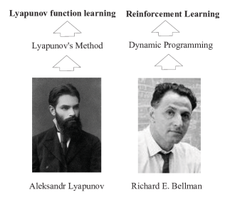
Figure 1: Lyapunov function learning v.s. RL.

(i) Principle. As a solution to optimal control problems forward-in-time, RL often focuses on optimization based on the Bellman equation. In the traditional control field, the Bellman equation is often used as an analysis tool rather than a direct design tool in optimization control. However, the hand-design Lyapunov’s method, depending on pseudo-energy functions, is the most popular tool in both analysis and design, aiming to decrease pseudo-energy functions over time so that the state converges to a fixed point. Technically, RL is required to define the rewards function and compute the value function (optimal objectives are defined as priors). In contrast, Lyapunov function learning requires training a parameterized Lyapunov function to match the data set (concrete Lyapunov functions are NOT defined as priors). Therefore, they are different in both application and design. RL with Lyapunov functions, where certificates are used to ensure safety or stability, has also been proposed recently. A commonly used certificate is the sum of cost over a limited time horizon as a valid Lyapunov candidate [7]. Compared RL with Lyapunov functions, Lyapunov function learning is more flexible in choosing candidates.

(ii) Applications. RL based on the Bellman equation is prevalent in the field of computer science due to its model-free characteristics. More importantly, it can solve very complicated control problems, such as playing Go [8], playing games [9] and magnetic control of tokamak plasmas [10]. Compared with RL, Lyapunov’s methods’ achievements on complicated problems with big data are less. Because of the big gap between developments by the Lyapunov’s method and the Bellman equation, it is hypothesized that there is an increasing focus on Lyapunov function learning from data. The expectation is to unveil its enormous potential, which is also the major motivation of this paper.

Constructing Lyapunov functions from data is related to:

(i) Lyapunov-stable neural-network control [11], neural Lyapunov control [12] and Learning-based robust neuro-control [13] employ neural networks to construct both Lyapunov functions and controller simultaneously;

(ii) Demonstration learning [14],[15], episodic Learning [16], and imitation learning [17] aim at only searching for a certificate from given control policy data.

From the examples in the existing literature, it is still far from complicated applications with big data. To this end, we hope to propose a new approach, namely control with patterns (CWP), working on some complicated applications with big data. This method follows the line of constructing both Lyapunov functions and controller simultaneously but focuses on the state and references expressed in the form of features [18] NOT limited to clear physical variables. Concretely, it processes the following characteristics.

(i) More Pattern Classification. i) Features. Unstructured data, such as images, videos, and sounds, are hard to express with clear physical variables. Due to this, features are abstracted from patterns in the form of a state or a set as feedback. For example, a hovering drone is stabilized by aligning the real-time obtained image to the reference images, namely image-based visual servoing [19], without reconstructing the relative pose. State-of-the-art methods rely on the corner point and their correspondence, which suffer from no-corner-point and mismatching problems [20]. ii) Negative samples (or counterexamples). So far, some existing methods also use counterexamples from model-based optimization to cast the construction of the Lyapunov function problem as a pattern-classified problem [15],[21]. In the new method, more negative samples are expected to be generated from data that could follow the idea of rewards in RL. For example, suppose a drone hits an obstacle or converges to a wrong equilibrium through a series of actions and states. In that case, the series of actions and states will be punished by labeling with a negative weight within the range of [-1,0]. Due to the two characters mentioned above, more methods in pattern classification are applicable.

(ii) More Control. i) Online adaption. Most methods related to constructing Lyapunov functions from data are offline. They cannot handle varying uncertainties in practice. ii) More control theory and problems. Existing studies on Lyapunov function learning often consider stabilizing control. Apparently, non-minimum phase system tracking with data is challenging [22] because it is not only a Lyapunov function constructing problem. Many theories in the field of control, like the internal model principle [23], [24], could be adopted. Owing to the two characters mentioned above, more control methods are expected to bring in learning with data.

In a word, we hope the CWP bridges control theory and machine learning, exploring its enormous potential in solving complicated applications with big data. First, this paper proposes problem formulation with an outline of CWP. Then, D-learning is proposed parallel to Q-learning [25] in RL to obtain both Lyapunov functions and controller simultaneously. Unlike existing Lyapunov function learning methods relying on controlled models or their approximation with neural networks [11], the system dynamics are encoded into the so-called D function (a scalar) depending on actions. This allows one to perform CWP without any knowledge of the system dynamics.

The contributions of this paper are as follows.

(i) A new framework related to Lyapunov function learning, coined as CWP, is proposed, where the feature abstraction has to be considered for unstructured data feedback.

(ii) D-learning is proposed to perform CWP without prior knowledge of the system dynamics.

II Problem Formulation

II-A System Conversion

Consider the following autonomous system

$$\mathbf{\dot{x}}^{\prime} =\mathbf{f}^{\prime}\left(\mathbf{x}^{\prime}\right)$$

$$\mathbf{x} =\mathbf{s}\left(\mathbf{m}\left(\mathbf{x}^{\prime}\right)\right)$$

where $\mathbf{x}^{\prime}\in\mathcal{D}^{\prime}\subseteq\mathbb{R}^{n^{\prime}}$ is original state unavailable to measure, $\mathbf{m}\left(\mathbf{x}^{\prime}\right)\in\mathcal{M}$ is a measurement in the form of unstructured data such as images, and $\mathbf{s}\left(\cdot\right)$ is a designed feature selection function to code the measurement to a vector $\mathbf{x}\in\mathcal{D}\subseteq\mathbb{R}^{n}.$

Lemma 1. If $\left(\mathbf{s\circ m}\right)^{-1}:\mathcal{D\rightarrow D}^{\prime}$ exists and is local Lipschitz at neighbourhood around $\mathbf{x}^{\ast}$, then $\mathbf{x}\left(t\right)\rightarrow\mathbf{x}^{\ast}$ implies $\mathbf{x}^{\prime}\left(t\right)\rightarrow\left(\mathbf{s\circ m}\right)^{-1}\left(\mathbf{x}^{\ast}\right)$ as $t\rightarrow\mathbf{\infty.}$

Proof. At neighbourhood around $\mathbf{x}^{\ast},$ if $\left(\mathbf{s\circ m}\right)^{-1}:\mathcal{D\rightarrow D}^{\prime}$ exists, then

$$\mathbf{x}^{\prime} =\left(\mathbf{s\circ m}\right)^{-1}\left(\mathbf{x}\right)$$

$$\mathbf{x}^{\prime\mathbf{\ast}} =\left(\mathbf{s\circ m}\right)^{-1}\left(\mathbf{x}^{\ast}\right).$$

If $\left(\mathbf{s\circ m}\right)^{-1}$ is local Lipschitz at neighbourhood around $\mathbf{x}^{\ast}\mathbf{,}$ then there exists a gain $L^{\ast}$ at neighbourhood around $\mathbf{x}^{\ast}$ such that

$$\left\|\mathbf{x}^{\prime}-\mathbf{x}^{\prime\mathbf{\ast}}\right\|\leq L^{\ast}\left\|\mathbf{x-x}^{\ast}\right\|.$$

With the inequality above, $\mathbf{x}\left(t\right)\rightarrow\mathbf{x}^{\ast}$ implies $\mathbf{x}^{\prime}\left(t\right)\rightarrow\left(\mathbf{s\circ m}\right)^{-1}\left(\mathbf{x}^{\ast}\right)$ as $t\rightarrow\mathbf{\infty.}$ $\square$

Theorem 1. If $\left(\mathbf{s\circ m}\right)^{-1}:\mathcal{D\rightarrow D}^{\prime}$ exists and is local Lipschitz at $\mathcal{D}$, then $\mathbf{x}\left(t\right)\rightarrow\mathbf{x}^{\ast}$ implies $\mathbf{x}^{\prime}\left(t\right)\rightarrow\left(\mathbf{s\circ m}\right)^{-1}\left(\mathbf{x}^{\ast}\right)$ as $t\rightarrow\mathbf{\infty}$ for $\forall\mathbf{x}^{\ast}\in\mathcal{D}\mathbf{.}$

Proof. It is a direct result from Lemma 1. $\square$

Lemma 1 is a local result while Theorem 1 is a global one. If $\mathbf{s}^{-1}\$and $\mathbf{m}^{-1}$ both exist and are local Lipschitz, then $\left(\mathbf{s\circ m}\right)^{-1}$ exists and is local Lipschitz. But, the condition is more conservative. Given that accessing $\mathbf{m}\left(\mathbf{x}^{\prime}\right)$ is relatively straightforward, whereas obtaining $\mathbf{m}^{-1}$ is challenging or time-consuming, and sometimes only $\mathbf{m}\left(\mathbf{x}^{\prime\mathbf{\ast}}\right)$ is provided as a reference, we aim to focus on $\mathbf{x}$ rather than $\mathbf{x}^{\prime},$ namely considering the following autonomous system

$$\mathbf{\dot{x}} =\left.\frac{\partial\mathbf{s}}{\partial\mathbf{m}}\frac{\partial\mathbf{m}}{\partial\mathbf{x}^{\prime}}\mathbf{f}^{\prime}\left(\mathbf{x}^{\prime}\right)\right|_{\mathbf{x}^{\prime}=\left(\mathbf{s\circ m}\right)^{-1}\left(\mathbf{x}\right)}$$

$$\triangleq\mathbf{f}\left(\mathbf{x}\right),\mathbf{x}\left(0\right)=\mathbf{x}_{0}\in\mathcal{D}$$ (1)

where $\mathbf{f}:\mathcal{D}\rightarrow\mathbb{R}^{n}.$ Without loss of the generality, let

$$\mathbf{f}^{\prime}\left(\mathbf{0}\right)=\mathbf{0,s}\left(\mathbf{m}\left(\mathbf{0}\right)\right)=\mathbf{0.}$$

Then $\mathbf{f}\left(\mathbf{0}\right)=\mathbf{0}.$

Remark 1 (on feature selection function). The state $\mathbf{x}^{\prime}$ may be the position and attitude of a drone, while $\mathbf{m}\left(\mathbf{x}^{\prime}\right)$ is an image that the drone takes at the state $\mathbf{x}^{\prime}.$ If the image consists of repeated patterns, it is not easy to obtain $\mathbf{x}^{\prime}$ from $\mathbf{m}\left(\mathbf{x}^{\prime}\right).$ For the visual servoing problem, image $\mathbf{m}\left(\mathbf{x}^{\prime\mathbf{\ast}}\right)$ is given as a reference, but it is not easy to define the distance between two images for control. This is why the feature selection function is proposed to measure the distance between two images. A direct idea of choosing the feature selection function is to make

$$\mathbf{s\circ m}=\mathbf{I}_{n}$$

so that $\mathbf{x}^{\prime}=\mathbf{x.}$ This implies $\mathbf{s}=\mathbf{m}^{-1}\$but it is not easy to find as mentioned above. On the other hand, we hope the designed feature selection function can make the problem more tractable. For example, Koopman theory [26] provides a perspective to analyze nonlinear dynamical systems under a linear framework. Motivated by it, $\mathbf{f}$ could be designed as a linear operator by choosing $\mathbf{s}$. In the following, let us set aside the discussion on how to design a feature selection function for now and shift our focus to the stability and stabilizing problem with data.

II-B Problem Formulation

The data set

$$\mathcal{P}=\left\{\left(\mathbf{\dot{x}}_{i}\mathbf{,x}_{i}\right),i=1,\cdots,N\right\}$$ (2)

which is an observation from the unknown autonomous system (1). Before introducing the objective, some definitions are given related to the system (1) and the data set (2).

Definition 1 (Exponentially Stable). For the autonomous system (1), an equilibrium state $\mathbf{x}=\mathbf{0}_{n\times 1}$ is exponentially stable if there exist $\alpha,\lambda\in\mathbb{R}_{+}$ such that $\left\|\mathbf{\phi}\left(\tau;0,\mathbf{x}_{0}\right)\right\|\leq\alpha\left\|\mathbf{x}_{0}\right\|e^{-\lambda\tau}$ in some neighborhoods around the origin. Global exponential stability is independent of the initial state $\mathbf{x}_{0}.$

Here, $\mathbf{\phi}\left(\tau;0,\mathbf{x}_{0}\right)$ represents the solution starting at $\mathbf{x}_{0},$ $\tau\geq 0.$ It should be noted that we can only use the data set (2). So, a new definition related to stability, especially for the data set is proposed in the following.

Definition 2 (Exponentially Attractive on $\mathcal{P}$). For the autonomous dynamics (1), an equilibrium state $\mathbf{x}=\mathbf{0}_{n\times 1}$ is exponentially attractive on the data set $\mathcal{P}$ with $\alpha,\lambda,\varepsilon,\delta$ $\in\mathbb{R}_{+}$ if $\left\|\mathbf{\phi}\left(\tau;0,\mathbf{x}\right)\right\|\leq\alpha\left\|\mathbf{x}\right\|e^{-\lambda\tau},$ $\forall\tau\in\left[0,\delta\right],$ $\forall\mathbf{x}\in\mathcal{B}\left(\mathbf{x}_{i},\varepsilon\right)$ for any $\mathbf{x}_{i}\in\mathcal{P}$, where $\mathcal{B}\left(\mathbf{x}_{i},\varepsilon\right)$ denotes a neighborhood around $\mathbf{x}_{i}$ with radius $\varepsilon$.

Definition 2 is to describe the trajectory of the autonomous system (1) starting from the state. It is hard or impossible to get the exponential stability only based on the data set (2) except for more information on $\mathbf{f}\left(\mathbf{x}\right)$ obtained further. So, the definition of exponential attraction especially for the data set can be served as an intermediate result for classical stability results. For some special systems, we can build the relationship between the exponential stability and exponential attraction.

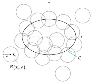
Figure 2: $\mathcal{C}_{l}$ belongs to the collection of $\mathcal{B}\left(\mathbf{x}_{i},\varepsilon\right)$.

Theorem 2. For the autonomous dynamics $\mathbf{\dot{x}}=\mathbf{Ax}$, suppose i) the equilibrium state $\mathbf{x}=\mathbf{0}_{n\times 1}$ is exponential attractive on the data set $\mathcal{P}$ with $\varepsilon$, ii) as shown in Fig.2, $\exists\ l\in\mathbf{\mathbb{R}}_{+}$, $\mathcal{C}_{l}\subseteq\cup_{i}\mathcal{B}\left(\mathbf{x}_{i},\varepsilon\right),$ $\mathbf{x}_{i}\in\mathcal{P}$, where $\mathcal{C}_{l}=\left\{\left.\mathbf{x}\in\mathcal{D}\right|\mathbf{x}^{\text{T}}\mathbf{Px}=l\right\}$ for a positive-definite matrix $\mathbf{0}<\mathbf{P}=\mathbf{P}^{\text{T}}\in\mathbb{R}^{n\times n}.$ Then the equilibrium state $\mathbf{x}=\mathbf{0}_{n\times 1}$ is globally exponential stability.

Proof. For any $\mathbf{x}^{\mathbf{\ast}}\neq\mathbf{0}_{n\times 1}\in\mathbf{\mathbb{R}}^{n}\mathbf{,}$ since $\mathbf{x}^{\mathbf{\ast}\text{T}}\mathbf{\mathbf{P}x}^{\mathbf{\ast}}\neq 0$ due to $\mathbf{P}$ being a positive-definite matrix, we have

$$\mathbf{\bar{x}}^{\mathbf{\ast}}=\theta\mathbf{x}^{\mathbf{\ast}}\in\mathcal{C}_{l}$$

where $\theta=\sqrt{\frac{l}{\mathbf{x}^{\mathbf{\ast}}\mathbf{{}^{\text{T}}\mathbf{P}x}^{\mathbf{\ast}}}}.$ Since $\mathbf{\phi}\left(\tau;0,\mathbf{x}\right)=e^{\mathbf{A}\tau}\mathbf{x,}$ for $\mathbf{\bar{x}}^{\mathbf{\ast}}\in\mathcal{C}_{l},$ the solution is $\mathbf{\phi}\left(\tau;0,\mathbf{\bar{x}}^{\mathbf{\ast}}\right)$ satisfying

$$\mathbf{\phi}\left(\tau;0,\mathbf{\bar{x}}^{\mathbf{\ast}}\right)=\theta\mathbf{\phi}\left(\tau;0,\mathbf{x}^{\mathbf{\ast}}\right).$$

On the other hand, since the equilibrium state $\mathbf{x}=\mathbf{0}_{n\times 1}$ is exponential attractive on the data set $\mathcal{P}$ with $\varepsilon,$ there exist $\alpha,\lambda,\varepsilon,\delta$ $\in\mathbb{R}_{+}$ such that $\left\|\mathbf{\phi}\left(\tau;0,\mathbf{\bar{x}}^{\mathbf{\ast}}\right)\right\|\leq\alpha\left\|\mathbf{\bar{x}}^{\mathbf{\ast}}\right\|e^{-\lambda\tau},$ $\forall\tau\in\left[0,\delta\right].$ Therefore,

$$\left\|\mathbf{\phi}\left(\tau;0,\mathbf{x}^{\mathbf{\ast}}\right)\right\| =\frac{1}{\theta}\left\|\mathbf{\phi}\left(\tau;0,\mathbf{\bar{x}}^{\mathbf{\ast}}\right)\right\|$$

$$\leq\frac{\alpha}{\theta}\left\|\mathbf{\bar{x}}^{\mathbf{\ast}}\right\|e^{-\lambda\tau}$$

$$=\alpha\left\|\mathbf{x}^{\mathbf{\ast}}\right\|e^{-\lambda\tau}$$

$\forall\tau\in\left[0,\delta\right],$ $\forall\mathbf{x}\in\mathcal{B}\left(\mathbf{x}^{\mathbf{\ast}},\varepsilon\right)$ for any $\mathbf{x}_{i}\in\mathcal{P}.$ Therefore, the equilibrium state $\mathbf{x}=\mathbf{0}_{n\times 1}$ is globally exponentially stable. $\square$

Problem Formulation. The first objective is to check whether $\mathbf{x}=\mathbf{0}_{n\times 1}$ is exponentially attractive on the data set (2). The other is to design a controller to make $\mathbf{x}=\mathbf{0}_{n\times 1}$ of the closed-loop system with data set (2) exponentially attractive.

Remark 2. Theorem 2 implies that, for autonomous linear dynamics, exponential attraction is equivalent to exponential stability if the data sets cover the boundary of an ellipsoid. For general dynamics, the least amount of data required for the equivalence is worth studying. Some research has applied statistical learning theory to provide probabilistic upper bounds on the generalization error, but these bounds tend to be overly cautious [5].

III Stability Problem as Pattern Classification

III-A Problem Conversion

We prepare to solve the exponential attraction problem using the Lyapunov method. The Lyapunov function for the data set (2) is supposed to have the following form

$$V\left(\mathbf{x}\right)=\mathbf{g}\left(\mathbf{x}\right)^{\text{T}}\boldsymbol{\theta}_{g}$$ (3)

where $V\left(\mathbf{0}_{n\times 1}\right)=0$, $V:\mathcal{D}/\left\{\mathbf{0}_{n\times 1}\right\}\rightarrow\mathcal{\mathbb{R}}_{+}$ and $\boldsymbol{\theta}_{g}\in\mathcal{S}_{g}\subseteq\mathbb{R}^{l_{1}}.$ The set $\mathcal{S}_{g}$ is used to guarantee that the function $V\left(\mathbf{x}\right)$ is a Lyapunov function. The derivative of $V\left(\mathbf{x}\right)$ yields

$$\dot{V}\left(\mathbf{x}\right)=\left(\frac{\partial\mathbf{g}\left(\mathbf{x}\right)}{\partial\mathbf{x}}\mathbf{\dot{x}}\right)^{\text{T}}\boldsymbol{\theta}_{g}.$$ (4)

We hope that the derivative satisfies

$$\dot{V}\left(\mathbf{x}\right)\leq-W\left(\boldsymbol{\theta}_{h},\mathbf{x}\right)$$ (5)

where $W\left(\boldsymbol{\theta}_{h},\mathbf{x}\right)$ is also a Lyapunov function, which can be further written as

$$W\left(\mathbf{x}\right)=\mathbf{h}\left(\mathbf{x}\right)^{\text{T}}\boldsymbol{\theta}_{h}$$

where $\boldsymbol{\theta}_{h}\in\mathcal{S}_{h}\subseteq\mathbb{R}^{l_{2}}.$ Similarly, the set $\mathcal{S}_{g}$ is used to guarantee that the function $W\left(\mathbf{x}\right)$ is a Lyapunov function as well.

For the data set (2), suppose that we have

$$\left(\left.\frac{\partial\mathbf{g}\left(\mathbf{x}\right)}{\partial\mathbf{x}}\right|_{\mathbf{x}=\mathbf{x}_{i}}\mathbf{\dot{x}}_{i}\right)^{\text{T}}\boldsymbol{\theta}_{g}\leq-\mathbf{h}\left(\mathbf{x}_{i}\right)^{\text{T}}\boldsymbol{\theta}_{h}$$ (6)

where $i=1,\cdots,N.$ Then, in the following, based on (6), we will show that the equilibrium state $\mathbf{x}=\mathbf{0}_{n\times 1}$ is exponentially attractive on the data set $\mathcal{P}.$ Before it, some assumptions are made.

Assumption 1. For $\mathbf{x}\in\mathcal{D},$ $\left\|\mathbf{x}\right\|\leq d$, where $d\in\mathbb{R}_{+}$.

Assumption 2. For $\mathbf{x}\in\mathcal{D},$ the function $\mathbf{f}$ satisfies $\left\|\partial\mathbf{f}\left(\mathbf{x}\right)\left/\partial\mathbf{x}\right.\right\|\leq l_{f}$, where $l_{f}\in\mathbb{R}_{+}$.

Assumption 3. For $\mathbf{x}_{1},\mathbf{x}_{2}\in\mathcal{D},$ there exists $l_{g}\in\mathbb{R}_{+}$ such that

$$\left\|\left.\partial\mathbf{g}\left(\mathbf{x}\right)\left/\partial\mathbf{x}\right.\right|_{\mathbf{x}=\mathbf{x}_{1}}-\left.\partial\mathbf{g}\left(\mathbf{x}\right)\left/\partial\mathbf{x}\right.\right|_{\mathbf{x}=\mathbf{x}_{2}}\right\|\leq l_{g}\left\|\mathbf{x}_{1}-\mathbf{x}_{2}\right\|.$$

Assumption 4. For $\mathbf{x}\in\mathcal{D},$ there exist $k_{1},k_{2}\in\mathbb{R}_{+}$ such that $k_{1}\left\|\mathbf{x}\right\|^{2}\leq\left\|\mathbf{g}\left(\mathbf{x}\right)^{\text{T}}\boldsymbol{\theta}_{g}\right\|\leq k_{2}\left\|\mathbf{x}\right\|^{2}.$

Assumption 5. For $\mathbf{x}\in\mathcal{D},$ there exists a $k_{3}\in\mathbb{R}_{+}$ such that $k_{3}\left\|\mathbf{x}\right\|^{2}<\mathbf{h}\left(\mathbf{x}\right)^{\text{T}}\boldsymbol{\theta}_{h}.$

Theorem 3. Under Assumptions 1-5, for the autonomous system (1), if there exist parameter vectors $\boldsymbol{\theta}_{g}\in\mathcal{S}_{g}\emph{\ }$and $\boldsymbol{\theta}_{h}\in\mathcal{S}_{h}$ such that (6) holds for the data set $\mathcal{P}$, then the equilibrium state $\mathbf{x}=\mathbf{0}_{n\times 1}$ is exponentially attractive on the data set $\mathcal{P}.$

Proof. See Appendix. $\square$

Assumptions 1-2 are easy to satisfy for most systems because the set $\mathcal{D}$ is bounded. Assumptions 3-5 are related to the Lyapunov functions on bounded set $\mathcal{D}$. Consequently, according to Theorem 3, the exponential attraction problem is converted to make the inequality (6) hold. The inequality (6) is rewritten as

$$\mathbf{y}_{i}^{\text{T}}\boldsymbol{\theta}\geq 0,i=1,\cdots,N$$ (7)

where

$$\mathbf{y}_{i} =-\left[\begin{array}[c]{cc}\left(\left.\frac{\partial\mathbf{g}\left(\mathbf{x}\right)}{\partial\mathbf{x}}\right|_{\mathbf{x}=\mathbf{x}_{i}}\mathbf{\dot{x}}_{i}\right)^{\text{T}}&\mathbf{h}\left(\mathbf{x}_{i}\right)^{\text{T}}\end{array}\right]^{\text{T}}$$

$$\boldsymbol{\theta} =\left[\begin{array}[c]{c}\boldsymbol{\theta}_{g}\\ \boldsymbol{\theta}_{h}\end{array}\right]\in\mathcal{S}\triangleq\mathcal{S}_{g}\times\mathcal{S}_{h}.$$

Formally, according to Theorem 3, the exponential attraction problem is converted as follows

$$\emph{For\ the\ data\ set\ (\ref{data set}),\ find\ }\boldsymbol{\theta}\in\mathcal{S}\text{ }\emph{to\ make}\text{ }\emph{(\ref{inequality1})\ hold.}$$

This problem is a pattern classification problem. Here, $\mathbf{y}_{i}$ is the compound features which describe the stability pattern for the autonomous system (1). As a result, $f\left(\boldsymbol{\theta}\right)=\mathbf{y}^{\text{T}}\boldsymbol{\theta}$ can be considered as a linear discriminant function [18]. The problem can be formulated into an optimization problem, such as

$$\begin{array}[c]{ll}\underset{\boldsymbol{\theta}\in\mathcal{S}}{\min}&a\\ \text{s.t.}&\begin{array}[c]{l}\mathbf{y}_{i}^{\text{T}}\boldsymbol{\theta}\geq 0,i=1,\cdots,N\\ F\left(\boldsymbol{\theta}\right)\leq a\end{array}\end{array}$$ (8)

where $F\left(\boldsymbol{\theta}\right)$ is a constraint on $\boldsymbol{\theta}.$ However, the real data may be subject to noise and “outliers” that do not fit the inequality (6). In this case, no solution may be found.

The convergence rate is expected to make as large as possible. For simplicity, let $W\left(\boldsymbol{\theta}_{h},\mathbf{x}\right)=\eta\left\|\mathbf{x}\right\|^{2}$ in the following. The inequality (5) is rewritten as

$$\dot{V}\left(\mathbf{x}\right)\leq-\eta\left\|\mathbf{x}\right\|^{2}$$ (9)

where $\eta\in\mathbb{R}.$ According to this, the optimization problem (8) is modified as

$$\begin{array}[c]{ll}\underset{\boldsymbol{\theta}_{g}\in\mathcal{S}_{g},a>0}{\min}&wa-\eta\\ \text{s.t.}&\begin{array}[c]{l}-\left(\left.\frac{\partial\mathbf{g}\left(\mathbf{x}\right)}{\partial\mathbf{x}}\right|_{\mathbf{x}=\mathbf{x}_{i}}\mathbf{\dot{x}}_{i}\right)^{\text{T}}\boldsymbol{\theta}_{g}-\eta\left\|\mathbf{x}_{i}\right\|^{2}\geq 0,i=1,\cdots,N\\ F_{g}\left(\boldsymbol{\theta}_{g}\right)\leq a.\end{array}\end{array}$$ (10)

One of the objectives is to increase $\eta$ as large as possible. Without noise, the value $\eta$ should be positive.

III-B An Illustration Example

In the following, we consider commonly-used linear-quadratic Lyapunov functions. It should be noticed that such Lyapunov functions apply to both linear systems and nonlinear systems. For the data set (2), a linear-quadratic Lyapunov function is supposed to have the following form

$$V\left(\mathbf{x}\right)=\mathbf{x}^{\text{T}}\mathbf{Px}$$ (11)

where $\mathbf{0}<\mathbf{P}=\mathbf{P}^{\text{T}}\in\mathbb{R}^{n\times n}$ is a positive-definite matrix. The derivative of $V\left(\mathbf{x}\right)$ yields

$$\dot{V}\left(\mathbf{x}\right)=\mathbf{\dot{x}}^{\text{T}}\mathbf{Px}+\mathbf{x}^{\text{T}}\mathbf{P\dot{x}}.$$

We hope that the derivative satisfies

$$\mathbf{\dot{x}}^{\text{T}}\mathbf{Px}+\mathbf{x}^{\text{T}}\mathbf{P\dot{x}}\leq-\eta\mathbf{x}^{\text{T}}\mathbf{x.}$$ (12)

Based on the data set (2), the inequality (12) becomes

$$\mathbf{\dot{x}}_{i}^{\text{T}}\mathbf{Px}_{i}+\mathbf{x}_{i}^{\text{T}}\mathbf{P\dot{x}}_{i}\leq-\eta\mathbf{x}_{i}^{\text{T}}\mathbf{x}_{i}$$ (13)

where $i=1,\cdots,N.$ The inequality (13) is further written as (7) with

$$\mathbf{y}_{i} =-\left[\begin{array}[c]{cc}\mathbf{x}_{i}^{\text{T}}\otimes\mathbf{\dot{x}}_{i}^{\text{T}}+\mathbf{\dot{x}}_{i}^{\text{T}}\otimes\mathbf{x}_{i}^{\text{T}}&\mathbf{x}_{i}^{\text{T}}\otimes\mathbf{x}_{i}^{\text{T}}\end{array}\right]^{\text{T}}$$

$$\boldsymbol{\theta} =\left[\begin{array}[c]{c}\text{vec}\left(\mathbf{P}\right)\\ \eta\text{vec}\left(\mathbf{I}_{n}\right)\end{array}\right]\in\mathbb{R}^{2n^{2}\times 1}.$$

To avoid a trivial solution such as $\boldsymbol{\theta}=\mathbf{0}_{2n^{2}\times 1}\mathbf{,}$ some constraints have to be imposed on the vector $\boldsymbol{\theta}.$ For example,

$$\boldsymbol{\theta}\in\mathcal{S}_{p}=\left\{\left.\mathbf{z}\in\mathbb{R}^{2n^{2}\times 1}\right|\mathbf{z}=\left[\begin{array}[c]{c}\text{vec}\left(\mathbf{P}\right)\\ \eta\text{vec}\left(\mathbf{I}_{n}\right)\end{array}\right]\right\}$$ (14)

with

$$\mathbf{0}<\mathbf{I}_{n}\leq\mathbf{P}=\mathbf{P}^{\text{T}}\leq a\mathbf{I}_{n}\in\mathbb{R}^{n\times n}.$$

According to (10), the exponential attraction problem can be formulated into an optimization problem, such as

$$\begin{array}[c]{ll}\underset{\eta,\mathbf{P},a>0}{\min}&wa-\eta\\ \text{s.t.}&\mathbf{\dot{x}}_{i}^{\text{T}}\mathbf{Px}_{i}+\mathbf{x}_{i}^{\text{T}}\mathbf{P\dot{x}}_{i}\leq-\eta\mathbf{x}_{i}^{\text{T}}\mathbf{x}_{i},i=1,\cdots,N\\ &\mathbf{0}<\mathbf{I}_{n}<\mathbf{P}=\mathbf{P}^{\text{T}}\leq a\mathbf{I}_{n}\in\mathbb{R}^{n\times n}\end{array}$$

where $w\in\mathbb{R}_{+\text{ }}$is a weight. This problem can be solved by a linear matrix inequality (LMI) techniques [31], such as YALMIP [32] and the LMI control toolbox.

IV Control with Patterns based on D-learning

After considering the stability problem, we are going to consider the control problem based on data sets.

IV-A Control Problem Formulation

Consider the following controlled system

$$\mathbf{\dot{x}}^{\prime} =\mathbf{f}^{\prime}\left(\mathbf{x}^{\prime},\mathbf{u}\right)$$

$$\mathbf{x} =\mathbf{s}\left(\mathbf{m}\left(\mathbf{x}^{\prime}\right)\right)$$

which can be converted into

$$\mathbf{\dot{x}}=\mathbf{f}\left(\mathbf{x,u}\right)$$ (15)

where $\mathbf{x}\in\mathcal{D}\subseteq\mathbb{R}^{n}$, $\mathbf{f}:\mathcal{D}\times\mathcal{U}\rightarrow\mathbb{R}^{n}$ and the control policy is defined as a function from

$$\mathbf{u}=\mathbf{c}\left(\mathbf{x}\right).$$

Consider the following data set

$$\mathcal{P}_{u}\left(\mathbf{c}\right)=\left\{\left(\mathbf{\dot{x}}_{i}\left(\mathbf{c}\right)\mathbf{,x}_{i}\right),i=1,\cdots,N\right\}$$ (16)

which is an observation from the controlled system (15). The control problem can be stated as follows

$$\text{\emph{Design} }\mathbf{u}\in\mathcal{U}\text{ \emph{and}}\emph{\ }\text{\emph{find} }\boldsymbol{\theta}\in\mathcal{S}\text{ \emph{to make\ (\ref{inequality1})}}\ \text{\emph{hold\ on the\ data\ set\ (\ref{data_con})}.}$$ (17)

The closed-loop is shown in Fig.3.

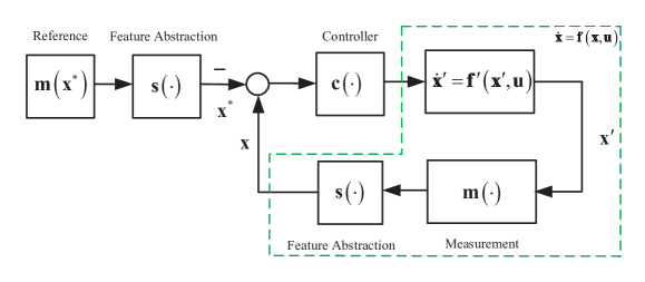
Figure 3: Closed-loop system by CWP.

IV-B Control with Patterns

In order to solve the control problem (17), we solve the following optimization

$$\begin{array}[c]{ll}\underset{\eta,\boldsymbol{\theta}_{g}\in\mathcal{S}_{g},a>0,\mathbf{c}}{\min}&wa-\eta\\ \text{s.t.}&\begin{array}[c]{l}-\left(\left.\frac{\partial\mathbf{g}\left(\mathbf{x}\right)}{\partial\mathbf{x}}\right|_{\mathbf{x}=\mathbf{x}_{i}}\mathbf{\dot{x}}_{i}\left(\mathbf{c}\right)\right)^{\text{T}}\boldsymbol{\theta}_{g}-\eta\left\|\mathbf{x}_{i}\right\|^{2}\geq 0\\ F_{g}\left(\boldsymbol{\theta}_{g}\right)\leq a\end{array}\end{array}$$ (18)

where$\ i=1,\cdots,N,$ where $F_{g}$ is a constraint on $\boldsymbol{\theta}_{g}.$ An iterative procedure for solving the inequality (18) may be used, including policy evaluation and policy improvement.

• Initialization. Select any admissible (i.e., stabilizing) control $\mathbf{c}_{0}$, $k=0$.

• Policy Evaluation Step. Under $\mathbf{c}_{k},$ at state $\mathbf{x}_{i},$ the control is $\mathbf{u}=\mathbf{c}_{k}\left(\mathbf{x}_{i}\right)\in\mathcal{U},$ resulting in $\mathbf{\dot{x}}_{i}\left(\mathbf{c}_{k}\right)\in\mathcal{D}$. Determine the solution $\boldsymbol{\theta}_{g,k},a>0,\eta_{k}$ by

  $$\begin{array}[c]{ll}\underset{\eta,\boldsymbol{\theta}_{g}\in\mathcal{S}_{g},a>0}{\min}&wa-\eta\\ \text{s.t.}&\begin{array}[c]{l}-\left(\left.\frac{\partial\mathbf{g}\left(\mathbf{x}\right)}{\partial\mathbf{x}}\right|_{\mathbf{x}=\mathbf{x}_{i}}\mathbf{\dot{x}}_{i}\left(\mathbf{c}\right)\right)^{\text{T}}\boldsymbol{\theta}_{g}-\eta\left\|\mathbf{x}_{i}\right\|^{2}\geq 0\\ F_{g}\left(\boldsymbol{\theta}_{g}\right)\leq a\end{array}\end{array}$$ (19)

  where $i=1,\cdots,N_{k}$.

• Policy Improvement Step. Determine an improved policy using

  $$\begin{array}[c]{ll}\underset{\mathbf{c,}\eta}{\min}&-\eta\\ \text{s.t.}&-\left(\left.\frac{\partial\mathbf{g}\left(\mathbf{x}\right)}{\partial\mathbf{x}}\right|_{\mathbf{x}=\mathbf{x}_{i}}\mathbf{\dot{x}}_{i}\left(\mathbf{c}\right)\right)^{\text{T}}\boldsymbol{\theta}_{g,k}-\eta\left\|\mathbf{x}_{i}\right\|^{2}\geq 0\end{array}$$ (20)

  where $i=1,\cdots,N_{k}$.

By fixing $\mathbf{x}_{i}\$for every step $k$, the iteration can be chosen to stop after sufficient steps if $wa_{k}-\eta_{k}$ and $-\eta_{k}$ are nearly not changed. This is because the iterative procedure is in fact used to solve the optimization (18) with the coordinate descent [34].

IV-C D-Learning

IV-C1 D function

Unfortunately, in the Policy Improvement Step, one requires knowledge of the system dynamics $\mathbf{\dot{x}}_{i}\left(\mathbf{c}\right)$. To avoid knowing any of the system dynamics, similar to Q-Learning [25],[36] in the field of RL, one can rewrite $\dot{V}\left(\mathbf{x}\right)$ in (4) as

$$D\left(\mathbf{x,u}\right)=\left(\frac{\partial\mathbf{g}\left(\mathbf{x}\right)}{\partial\mathbf{x}}\mathbf{f}\left(\mathbf{x,u}\right)\right)^{\text{T}}\boldsymbol{\theta}_{g}$$

where (15) is utilized. We call it the D (decreasing) function. If one obtains $D\left(\mathbf{x,u}\right)$ by learning directly, then the use of the input coupling function is avoided. In the nonlinear case, one assumes that the value of $D\left(\mathbf{x,u}\right)$ is sufficiently smooth. Then, according to the Weierstrass higher order approximation theorem, there exists a dense basis set $\left\{\varphi_{i}\left(\mathbf{x,u}\right)\right\}$ such that

$$D\left(\mathbf{x,u}\right) =\underset{i=1}{\overset{\infty}{{\displaystyle\sum}}}\theta_{i}\varphi_{i}\left(\mathbf{x,u}\right)$$

$$=\underset{i=1}{\overset{L}{{\displaystyle\sum}}}\theta_{i}\varphi_{i}\left(\mathbf{x,u}\right)+\underset{i=L+1}{\overset{\infty}{{\displaystyle\sum}}}\theta_{i}\varphi_{i}\left(\mathbf{x,u}\right)$$

$$\triangleq\boldsymbol{\theta}_{d}^{\text{T}}\boldsymbol{\phi}\left(\mathbf{x,u}\right)+\varepsilon_{L}\left(\mathbf{x,u}\right)$$

where basis vector $\boldsymbol{\theta}_{d}=[\theta_{1}$ $\theta_{2}$ $\cdots\ \theta_{L}]^{\text{T}},$ $\boldsymbol{\phi}\left(\mathbf{x,u}\right)=[\varphi_{1}\left(\mathbf{x,u}\right)$ $\varphi_{2}\left(\mathbf{x,u}\right)$ $\cdots$ $\varphi_{L}\left(\mathbf{x,u}\right)]^{\text{T}}$ and $\varepsilon_{L}$ converges uniformly to zero as the number of terms retained $L\rightarrow\infty.$ The following example is going to show D function. By (11), we have

$$D\left(\mathbf{x,u}\right) =2\mathbf{x}^{\text{T}}\mathbf{PAx+2\mathbf{x}}^{\text{T}}\mathbf{\mathbf{P}Bu}$$

$$=\boldsymbol{\theta}_{d}^{\text{T}}\boldsymbol{\phi}\left(\mathbf{x,u}\right)$$

where

$$\boldsymbol{\phi}\left(\mathbf{x,u}\right) =\left[\begin{array}[c]{cc}\mathbf{x}^{\text{T}}\otimes\mathbf{x}^{\text{T}}&\mathbf{x}^{\text{T}}\otimes\mathbf{u}^{\text{T}}\end{array}\right]^{\text{T}}$$

$$\boldsymbol{\theta}_{d} =\left[\begin{array}[c]{c}\text{vec}\left(\mathbf{PA}\right)\\ \text{vec}\left(\mathbf{\mathbf{P}B}\right)\end{array}\right].$$

IV-C2 D-Learning

Then (5) is rewritten as

$$\boldsymbol{\theta}_{d}^{\text{T}}\boldsymbol{\phi}\left(\mathbf{x,u}\right)\leq-W\left(\boldsymbol{\theta}_{h},\mathbf{x}\right).$$

Furthermore, the inequality (7) is rewritten as

$$\mathbf{y}_{i}^{\prime\text{T}}\boldsymbol{\theta}^{\prime}\geq 0,i=1,\cdots,N$$ (21)

where

$$\mathbf{y}_{i}^{\prime} =-\left[\begin{array}[c]{cc}\boldsymbol{\phi}\left(\mathbf{x}_{i}\mathbf{,u}_{i}\right)^{\text{T}}&\mathbf{h}\left(\mathbf{x}_{i}\right)^{\text{T}}\end{array}\right]^{\text{T}}$$

$$\boldsymbol{\theta}^{\prime} =\left[\begin{array}[c]{c}\boldsymbol{\theta}_{d}\\ \boldsymbol{\theta}_{h}\end{array}\right]\in\mathcal{S}^{\prime}\triangleq\mathbb{R}^{L}\times\mathcal{S}_{h}.$$

Meanwhile, it is expected to make $D\left(\mathbf{x,u}\right)-\dot{V}\left(\mathbf{x}\right)$ as small as possible. Mathematically, one has to decrease $b$ as small as possible with the following constraint

$$\left|\boldsymbol{\theta}_{d}^{\text{T}}\boldsymbol{\phi}\left(\mathbf{x}_{i},\mathbf{c}_{k}\left(\mathbf{x}_{i}\right)\right)-\boldsymbol{\theta}_{g}^{\text{T}}\left.\frac{\partial\mathbf{g}\left(\mathbf{x}\right)}{\partial\mathbf{x}}\right|_{\mathbf{x}=\mathbf{x}_{i}}\mathbf{\dot{x}}_{i}\left(\mathbf{c}_{k}\left(\mathbf{x}_{i}\right)\right)\right|\leq b$$

where $i=1,\cdots,N_{k},$ $k=1,\cdots,M.$ With the D function, iterative procedures for solving the inequality (18) should be rewritten, including policy evaluation and policy improvement.

• Initialization. Select any admissible (i.e., stabilizing) control $\mathbf{c}_{0}$, $k=0$.

• Policy Evaluation Step. Under $\mathbf{c}_{k},$ at state $\mathbf{x}_{i},$ the control is $\mathbf{u}=\mathbf{c}_{k}\left(\mathbf{x}_{i}\right)\in\mathcal{U},$ resulting in $\mathbf{\dot{x}}_{i}\left(\mathbf{c}_{k}\right)\in\mathcal{D}$. Determine the solution $\boldsymbol{\theta}_{g,k},\boldsymbol{\theta}_{d,k},a_{k},b_{k}>0,\eta_{k}\in\mathbb{R}$ by

  $$\begin{array}[c]{ll}\underset{\boldsymbol{\theta}_{d}\in\mathbb{R}^{L},\boldsymbol{\theta}_{g}\in\mathcal{S}_{g},a,b>0,\eta\in\mathbb{R}}{\min}&-\eta+w_{1}a+w_{2}b\\ \text{s.t.}&-\boldsymbol{\theta}_{d}^{\text{T}}\boldsymbol{\phi}\left(\mathbf{x}_{i},\mathbf{c}_{k}\left(\mathbf{x}_{i}\right)\right)-\eta\left\|\mathbf{x}_{i}\right\|^{2}\geq 0\\ &\begin{array}[c]{l}\left|\boldsymbol{\theta}_{d}^{\text{T}}\boldsymbol{\phi}\left(\mathbf{x}_{i},\mathbf{c}_{j}\left(\mathbf{x}_{i}\right)\right)-\boldsymbol{\theta}_{g}^{\text{T}}\left.\frac{\partial\mathbf{g}\left(\mathbf{x}\right)}{\partial\mathbf{x}}\right|_{\mathbf{x}=\mathbf{x}_{i}}\mathbf{\dot{x}}_{i}\left(\mathbf{c}_{j}\left(\mathbf{x}_{i}\right)\right)\right|\leq b\\ F_{g}\left(\boldsymbol{\theta}_{g}\right)\leq a\end{array}\end{array}$$ (22)

  where $w_{1},w_{2}>0$ are weights, $j=0,\cdots,k,i=1,\cdots,N_{k}$.

• Policy Improvement Step. Determine an improved policy using

  $$\begin{array}[c]{ll}\underset{\mathbf{c,}\eta\in\mathbb{R}}{\min}&-\eta\\ \text{s.t.}&-\boldsymbol{\theta}_{d,k}^{\text{T}}\boldsymbol{\phi}\left(\mathbf{x}_{i},\mathbf{c}_{k}\left(\mathbf{x}_{i}\right)\right)-\eta\left\|\mathbf{x}_{i}\right\|^{2}\geq 0\end{array}$$ (23)

  where $i=1,\cdots,N_{k}.$ In order to facilitate the optimization, we can parameterize $\mathbf{c}\left(\mathbf{x}\right)$ as

  $$\mathbf{c}\left(\mathbf{x}\right)=\boldsymbol{\Psi}\left(\mathbf{x}\right)\boldsymbol{\theta}_{c}$$

  where $\boldsymbol{\Psi}\left(\mathbf{x}\right)\in\mathbb{R}^{m\times p},\boldsymbol{\theta}_{c}\in\mathbb{R}^{p}.$ In this case, (23) can be rewritten as

  $$\begin{array}[c]{ll}\underset{\boldsymbol{\theta}_{c}\mathbf{,}\eta}{\min}&-\eta\\ \text{s.t.}&-\boldsymbol{\theta}_{d,k}^{\text{T}}\boldsymbol{\phi}\left(\mathbf{x}_{i},\boldsymbol{\Psi}\left(\mathbf{x}_{i}\right)\boldsymbol{\theta}_{c}\right)-\eta\left\|\mathbf{x}_{i}\right\|^{2}\geq 0,i=1,\cdots,N_{k}\end{array}.$$ (24)

IV-D How to Deal with Negative Samples

Consider the following negative samples set

$$\mathcal{P}_{n}=\left\{\left(\mathbf{\dot{x}}_{i_{n}}^{-}\mathbf{,x}_{i_{n}}^{-},c_{i_{n}}\right),i=1,\cdots,N_{n}\right\}$$ (25)

which is an observation from the control system (15). Negative samples could be sampled (easily) by violating constraints such as hitting an obstacle. Here, $c_{i}$ is the cost of the negative sample $\left(\mathbf{\dot{x}}_{i}^{-}\mathbf{,x}_{i}^{-}\right).$ For example, a drone hits an obstacle at time $t=t_{h}$. Similar to the RL, a discount factor $0<\gamma<1$ is introduced. Let the cost at $t=t_{h}$ be $1$. Then the cost of the negative sample at $t=t_{h}-kT_{s}$ is $\gamma^{k},$ where $T_{s}>0$ is the sample period. This implies that the cost is decreased as the drone is far from the obstacle. In practice, only samples with $c_{i}\geq c_{0}>0$ are selected as negative samples.

We hope that the derivative with these negative samples satisfies

$$\dot{V}\left(\mathbf{x}^{-}\right)\geq c_{i_{n}}W\left(\boldsymbol{\theta}_{h},\mathbf{x}^{-}\right).$$ (26)

In order to solve the control problem (17), similar to the inequality (18), we solve the following optimization

$$\begin{array}[c]{ll}\underset{\eta,\boldsymbol{\theta}_{g}\in\mathcal{S}_{g},a>0,\mathbf{c}}{\min}&wa-\eta\\ \text{s.t.}&\begin{array}[c]{l}-\left(\left.\frac{\partial\mathbf{g}\left(\mathbf{x}\right)}{\partial\mathbf{x}}\right|_{\mathbf{x}=\mathbf{x}_{i}}\mathbf{\dot{x}}_{i}\left(\mathbf{c}\right)\right)^{\text{T}}\boldsymbol{\theta}_{g}-\eta\left\|\mathbf{x}_{i}\right\|^{2}\geq 0,i=1,\cdots,N\\ \left(\left.\frac{\partial\mathbf{g}\left(\mathbf{x}\right)}{\partial\mathbf{x}}\right|_{\mathbf{x}=\mathbf{x}^{-}_{i_{n}}}\mathbf{\dot{x}}_{i_{n}}^{-}\right)^{\text{T}}\boldsymbol{\theta}_{g}-\eta c_{i_{n}}\left\|\mathbf{x}_{i_{n}}^{-}\right\|^{2}\geq 0,i_{n}=1,\cdots,N_{n}\\ F_{g}\left(\boldsymbol{\theta}_{g}\right)\leq a.\end{array}\end{array}$$ (27)

Based on the framework above, D-learning can be easily performed. Here, we omit it.

IV-E Discussions: Relationship between RL and CWP

IV-E1 Similarities

The similarities between RL and CWP lie in:

• They are both unsupervised learning aims at policy designing for dynamic systems.

• They both adopt the policy evaluation step and policy improvement step.

• The policy improvement of both aims to minimize the policy evaluation function.

IV-E2 Differences

As shown in Fig.4, the significant differences between RL and CWP lie in their definitions and objectives of the Lyapunov function and the cost function.

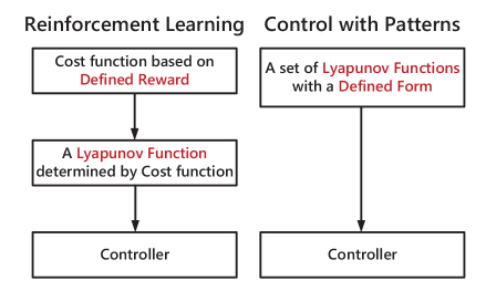
Figure 4: Different ways to determine Lyapunov functions.

• The Lyapunov function plays a crucial role in CWP rather than RL. Initially, it serves as a positive-definite function, attaining a minimum value of zero at the zero state. However, the cost function is based on the utility, which can also become a Lyapunov function by substituting the control policies into it. This implies that the utility has determined the Lyapunov function following Bellman’s optimality principle. It is worth noting that in some applications, the utility may take a negative value, which challenges the idea of designing the cost function in the form of a Lyapunov function. On the other hand, by CWP, the Lyapunov function is chosen more flexibly than RL. The only principle of choosing the Lyapunov function is to decrease its derivative so that the state converges to zero. Mathematically, inequalities by CWP rather than equality by RL are used to perform the policy evaluation step, where the former has a larger solution space. As a result, it is easier to obtain a solution to related problems by CWP.

• The objectives of the Lyapunov function and the cost function are also different. The former is required to design a policy to make the derivative of the Lyapunov function negative, while the latter is required to design a policy to minimize the cost function, a sum of discounted future costs from the current time into the infinite horizon future.

• The CWP is highly applicable when the desired state is known. With the desired state, the Lyapunov function can be established. However, RL is applicable to the case that the desired state is unknown, but the optimization objective is known. It is difficult to design an appropriate utility for RL. Similarly, it is also difficult to design an appropriate form of Lyapunov functions.

V Conclusions and Future Work

This paper proposes data sets representing features (Theorem 1) to describe autonomous and control systems. Within this context, a novel concept, exponential attraction, is introduced. The relationship between them for linear systems is clarified in Theorem 2. Furthermore, the relationship between the exponential attraction and the pattern classification problem (7) is clarified in Theorem 3. After that, we focus on the pattern classification problem. CWP based on D-learning for continuous-time systems is proposed, where the D function and iterative procedures are proposed to find the controller. However, many problems deserve further research in the future.

(i) Feature function and Lyapunov function. Deep neural networks can be used to construct these functions as well. This can extend the form proposed in this paper. What is more, the feature function, Lyapunov function, and controller in the form of deep neural networks could be learned together to perform better.

(ii) Data set. i) How to generate the data set by using fewer data to represent more information; ii) How to measure the difference between the data set and real system.

(iii) Stability related. i) The relationship between exponential stability and exponential attraction should be investigated further, especially for nonlinear systems. ii) Furthermore, the relationship between probability-related stability and exponential attraction should be established for a given data set.

VI Appendix

VI-A Proof of Theorem 3

This proof consists of three steps.

Step 1. $\left\|\Delta\mathbf{\dot{x}}_{i}\right\|\leq l_{f}\left\|\Delta\mathbf{x}_{i}\right\|.$ For any $\mathbf{x}\in\mathcal{B}\left(\mathbf{x}_{i},\varepsilon^{\prime}\right)$, it can be written as

$$\mathbf{x}=\mathbf{x}_{i}+\Delta\mathbf{x}_{i}$$

where $\mathbf{x}_{i}+\Delta\mathbf{x}_{i},\mathbf{x}_{i}\in\mathcal{D}$ and $\Delta\mathbf{x}_{i}\in\mathcal{B}\left(\mathbf{0},\varepsilon^{\prime}\right).$ Then $\left\|\Delta\mathbf{x}_{i}\right\|\leq\varepsilon^{\prime}$. In this case, we have

$$\mathbf{\dot{x}} =\mathbf{\dot{x}}_{i}+\Delta\mathbf{\dot{x}}_{i}=\mathbf{f}\left(\mathbf{x}_{i}+\Delta\mathbf{x}_{i}\right)\Rightarrow$$

$$\Delta\mathbf{\dot{x}}_{i} =\mathbf{f}\left(\mathbf{x}_{i}+\Delta\mathbf{x}_{i}\right)-\mathbf{f}\left(\mathbf{x}_{i}\right).$$

Under Assumption 2, we further have $\left\|\Delta\mathbf{\dot{x}}_{i}\right\|\leq l_{f}\left\|\Delta\mathbf{x}_{i}\right\|.$

Step 2. $\left\|\mathbf{\phi}\left(\tau;0,\mathbf{x}\right)\right\|\leq\alpha\left\|\mathbf{x}\right\|e^{-\lambda\tau}$ for $\forall\mathbf{x}\in\mathcal{B}\left(\mathbf{x}_{i},\varepsilon\right),$ where $\varepsilon=\varepsilon^{\prime}\left/2\right..$ For any $\mathbf{x}\in\mathcal{B}\left(\mathbf{x}_{i},\varepsilon^{\prime}\right),$ according to the definition of $V\left(\mathbf{x}\right)$ in (3), we have

$$\dot{V}\left(\mathbf{x}\right) =\left(\frac{\partial\mathbf{g}\left(\mathbf{x}\right)}{\partial\mathbf{x}}\mathbf{\dot{x}}\right)^{\text{T}}\boldsymbol{\theta}_{g}$$

$$=\left(\left.\frac{\partial\mathbf{g}\left(\mathbf{x}\right)}{\partial\mathbf{x}}\right|_{\mathbf{x}=\mathbf{x}_{i}+\Delta\mathbf{x}_{i}}\left(\mathbf{\dot{x}}_{i}+\Delta\mathbf{\dot{x}}_{i}\right)\right)^{\text{T}}\boldsymbol{\theta}_{g}$$

$$=\left(\left.\frac{\partial\mathbf{g}\left(\mathbf{x}\right)}{\partial\mathbf{x}}\right|_{\mathbf{x}=\mathbf{x}_{i}}\mathbf{\dot{x}}_{i}{\small+}\left.\frac{\partial\mathbf{g}\left(\mathbf{x}\right)}{\partial\mathbf{x}}\right|_{\mathbf{x}=\mathbf{x}_{i}+\Delta\mathbf{x}_{i}}\left(\mathbf{\dot{x}}_{i}+\Delta\mathbf{\dot{x}}_{i}\right)-\left.\frac{\partial\mathbf{g}\left(\mathbf{x}\right)}{\partial\mathbf{x}}\right|_{\mathbf{x}=\mathbf{x}_{i}}\mathbf{\dot{x}}_{i}\right)^{\text{T}}\boldsymbol{\theta}_{g}$$

$$=\left(\left.\frac{\partial\mathbf{g}\left(\mathbf{x}\right)}{\partial\mathbf{x}}\right|_{\mathbf{x}=\mathbf{x}_{i}}\mathbf{\dot{x}}_{i}+\left.\frac{\partial\mathbf{g}\left(\mathbf{x}\right)}{\partial\mathbf{x}}\right|_{\mathbf{x}=\mathbf{x}_{i}+\Delta\mathbf{x}_{i}}\mathbf{\dot{x}}_{i}-\left.\frac{\partial\mathbf{g}\left(\mathbf{x}\right)}{\partial\mathbf{x}}\right|_{\mathbf{x}=\mathbf{x}_{i}}\mathbf{\dot{x}}_{i}+\left.\frac{\partial\mathbf{g}\left(\mathbf{x}\right)}{\partial\mathbf{x}}\right|_{\mathbf{x}=\mathbf{x}_{i}+\Delta\mathbf{x}_{i}}\Delta\mathbf{\dot{x}}_{i}\right)^{\text{T}}\boldsymbol{\theta}_{g}$$

$$\leq-\mathbf{h}\left(\mathbf{x}_{i}\right)^{\text{T}}\boldsymbol{\theta}_{h}+l_{g}\left\|\Delta\mathbf{x}_{i}\right\|\left\|\mathbf{\dot{x}}_{i}\right\|\left\|\boldsymbol{\theta}_{g}\right\|+l_{g}\left\|\mathbf{x}_{i}+\Delta\mathbf{x}_{i}\right\|\left\|\Delta\mathbf{\dot{x}}_{i}\right\|\left\|\boldsymbol{\theta}_{g}\right\|\text{ ({From Assumption 3})}$$

$$\leq-\mathbf{h}\left(\mathbf{x}_{i}\right)^{\text{T}}\boldsymbol{\theta}_{h}+l_{g}l_{f}\left\|\boldsymbol{\theta}_{g}\right\|\left\|\mathbf{x}_{i}\right\|\varepsilon^{\prime}+l_{g}l_{f}\left\|\boldsymbol{\theta}_{g}\right\|\left(\left\|\mathbf{x}_{i}\right\|+\varepsilon^{\prime}\right)\varepsilon^{\prime}$$

$$\leq-\mathbf{h}\left(\mathbf{x}_{i}\right)^{\text{T}}\boldsymbol{\theta}_{h}+2l_{g}l_{f}\left\|\mathbf{x}_{i}\right\|\varepsilon^{\prime}+l_{g}l_{f}\varepsilon^{\prime 2}.$$

From Assumption 5, it is easy to obtain that $-\mathbf{h}\left(\mathbf{x}_{i}\right)^{\text{T}}\boldsymbol{\theta}_{h}+k_{3}\left\|\mathbf{x}_{i}\right\|^{2}<0$, then there exists a $\varepsilon^{\prime}\in\mathbb{R}_{+}$ such that $\dot{V}\left(\mathbf{x}\right)\leq-k_{3}\left\|\mathbf{x}\right\|^{2}.$ Then, by Assumption 4, we have

$$\dot{V}\left(\mathbf{x}\right)\leq-k_{3}\left\|\mathbf{x}\right\|^{2}\leq-2\lambda V\left(\mathbf{x}\right),\forall\mathbf{x}\in\mathcal{B}\left(\mathbf{x}_{i},\varepsilon^{\prime}\right)$$

where $\lambda=k_{3}\left/2k_{2}\right..$ Consequently, for $\mathbf{x}\in\mathcal{B}\left(\mathbf{x}_{i},\varepsilon\right),$ we have

$$V\left(\mathbf{\phi}\left(\tau;0,\mathbf{x}\right)\right)\leq\left\|V\left(\mathbf{x}\right)\right\|e^{-2\lambda\tau}$$

where $\tau\in\left[0,\tau^{\prime}\right]$ and $\tau^{\prime}$ is the first time that $\mathbf{\phi}\left(\tau;0,\mathbf{x}\right)\$is escaping out of $\mathcal{B}\left(\mathbf{x}_{i},\varepsilon^{\prime}\right)$. Note that $\mathcal{B}\left(\mathbf{x}_{i},\varepsilon\right)\subset\mathcal{B}\left(\mathbf{x}_{i},\varepsilon^{\prime}\right).$ As a result, by Assumption 4, we have

$$\left\|\mathbf{\phi}\left(\tau;0,\mathbf{x}\right)\right\|\leq\alpha\left\|\mathbf{x}\right\|e^{-\lambda\tau}$$

for $\mathbf{x}\in\mathcal{B}\left(\mathbf{x}_{i},\varepsilon\right),$ where $\alpha=\sqrt{k_{2}\left/k_{1}\right.}.$

Step 3. For any $\mathbf{x}\in\mathcal{B}\left(\mathbf{x}_{i},\varepsilon\right),$ the escaping time $\tau^{\prime}>\delta=\frac{\varepsilon}{l_{f}d}$. Under Assumptions 1-2, since

$$\mathbf{\phi}\left(\tau;0,\mathbf{x}\right)-\mathbf{x}={\displaystyle\int\nolimits_{0}^{\tau}}\mathbf{\dot{x}}\left(s\right)\text{d}s$$

we have

$$\left\|\mathbf{\phi}\left(\tau;0,\mathbf{x}\right)-\mathbf{x}\right\|\leq\tau^{\prime}\left\|\mathbf{f}\left(\mathbf{x}\right)\right\|\leq\tau^{\prime}l_{f}d.$$

The condition $\left\|\mathbf{\phi}\left(\tau;0,\mathbf{x}\right)-\mathbf{x}\right\|>\varepsilon=\varepsilon^{\prime}\left/2\right.$ implies that $\mathbf{\phi}\left(\tau;0,\mathbf{x}\right)\$is escaping out of $\mathcal{B}\left(\mathbf{x}_{i},\varepsilon^{\prime}\right).$ As a result, we have $\tau^{\prime}l_{f}d>\varepsilon$ and then $\tau^{\prime}>\delta.$

With Steps 1-3, there exist $\alpha=\sqrt{k_{2}\left/k_{1}\right.},$ $0<\lambda<k_{3}\left/2k_{2}\right.,$ $\varepsilon>0,$ and $\delta=\varepsilon\left/\left(l_{f}d\right)\right.$ such that $\left\|\mathbf{\phi}\left(\tau;0,\mathbf{x}\right)\right\|\leq\alpha\left\|\mathbf{x}\right\|e^{-\lambda\tau},$ $\forall\tau\in\left[0,\delta\right],$ $\forall\mathbf{x}\in\mathcal{B}\left(\mathbf{x}_{i},\varepsilon\right)$. Moreover, $\alpha,\lambda,\varepsilon$ and $\delta\$are independent of $\mathbf{x}_{i},$ so the result is applicable to any $\mathbf{x}_{i}\in\mathcal{P}.$ Therefore, the equilibrium state $\mathbf{x}=\mathbf{0}_{n\times 1}$ is exponentially attractive on the data set $\mathcal{P}.$

References

- [1] Levis, A. (1987). Challenges to Control: A Collective View–Report of the Workshop Held at the University of Santa Clara on September 18-19, 1986. IEEE Transactions on Automatic Control, vol. 32, no. 4, pp. 275–85, https://doi.org/10.1109/tac.1987.1104602.
- [2] Murray, R.M., Astrom, K.J., Boyd, S.P., Brockett, R.W., and Stein, G. (2003). Future Directions in Control in an Information-Rich World. IEEE Control Systems, vol. 23, pp. 20–33, https://doi.org/10.1109/mcs.2003.1188769.
- [3] Sutton, R.S. and Barto, A.G. (2012). Reinforcement learning: An introduction. The MIT Press, Cambridge.
- [4] Bertsekas, D.P. (2019). Reinforcement Learning and Optimal Control. Athena Scientific, 1st Edition.
- [5] Boffi, N.M., Tu, S., Matni, N., Slotine, J.-J., Sindhwani, V. (2020). Learning Stability Certificates from Data. Conference on Robot Learning, Held Virtually, November 16-18.
- [6] Dawson, C., Gao, S., & Fan, C. (2023). Safe Control With Learned Certificates: A Survey of Neural Lyapunov, Barrier, and Contraction Methods for Robotics and Control. IEEE Transactions on Robotics, vol. 39, no. 3, pp. 1749-1767, https://doi.org/10.1109/tro.2022.3232542.
- [7] Chow, Y., Nachum, O., Duenez-Guzman, E.A., & Ghavamzadeh, M. (2018). A Lyapunov-based Approach to Safe Reinforcement Learning. Neural Information Processing Systems, Montreal, Canada, December 2-8.
- [8] Silver, D., Schrittwieser, J., Simonyan, K., Antonoglou, I., Huang, A., Guez, A., Hubert, T., Baker, L., Lai, M., Bolton, A., Chen, Y., Lillicrap, T., Hui, F., Sifre, L., van den Driessche, G., Graepel, T., & Hassabis, D. (2017). Mastering the game of Go without human knowledge. Nature, vol. 550, no. 7676, pp. 354-359, https://doi.org/10.1038/nature24270.
- [9] Vinyals, O., Babuschkin, I., Czarnecki, W.M., Mathieu, M., Dudzik, A., Chung, J., Choi, D. H., Powell, R., Ewalds, T., Georgiev, P., Oh, J., Horgan, D., Kroiss, M., Danihelka, I., Huang, A., Sifre, L., Cai, T., Agapiou, J. P., Jaderberg, M., Vezhnevets, A. S., Leblond, R., Pohlen, T., Dalibard, V., Budden, D., Sulsky, Y., Molloy, J., Paine, T. L., Gulcehre, C., Wang, Z., Pfaff, T., Wu, Y., Ring, R., Yogatama, D., Wünsch, D., McKinney, K., Smith, Ol., Schaul, T., Lillicrap, T., Kavukcuoglu, K., Hassabis, D., Apps, C., & Silver, D. (2019). Grandmaster Level in StarCraft II Using Multi-agent Reinforcement Learning. Nature, vol. 575, no. 7782, pp. 350-354, https://doi.org/10.1038/s41586-019-1724-z.
- [10] Degrave, J., Felici, F., Buchli, J., Neunert, M., Tracey, B., Carpanese, F., Ewalds, T., Hafner, R., Abdolmaleki, A., de las Casas, D., Donner, C., Fritz, L., Galperti, C., Huber, A., Keeling, J., Tsimpoukelli, M., Kay, J., Merle, A., Moret, J., Noury, S., Pesamosca, F., Pfau, D., Sauter, O., Sommariva, C., Coda, S., Duval, B., Fasoli, A., Kohli, P., Kavukcuoglu, K., Hassabis, D., & Riedmiller, M. (2022). Magnetic Control of Tokamak Plasmas through Deep Reinforcement Learning. Nature, vol. 602, no. 7897, pp. 414-419, https://doi.org/10.1038/s41586-021-04301-9.
- [11] Dai, H., Landry, B., Yang, L., Pavone, M., & Tedrake, R. (2021). Lyapunov-Stable Neural-Network Control. Robotics: Science and Systems 2021, Held Virtually, July 12–16.
- [12] Chang, Y.-C., Roohi, N., & Gao, S. (2020). Neural Lyapunov Control. Neural Information Processing Systems, Held Virtually, December 6-12.
- [13] Rego, R.C.B., & de Araujo, F.M.U. (2022). Learning-Based Robust Neuro-Control: A Method to Compute Control Lyapunov Functions. International Journal of Robust and Nonlinear Control, vol. 32, no. 5, pp. 2644-2661, https://doi.org/10.1002/rnc.5399.
- [14] Neumann, K., Lemme, A., & Steil, J.J. (2013). Neural learning of stable dynamical systems based on data-driven Lyapunov candidates. 2013 IEEE/RSJ International Conference on Intelligent Robots and Systems, Tokyo, Japan, https://doi.org/10.1109/iros.2013.6696505.
- [15] Ravanbakhsh, H., & Sankaranarayanan, S. (2019). Learning Control Lyapunov Functions from Counterexamples and Demonstrations. Autonomous Robots, vol. 43, pp. 275–307. https://doi.org/10.1007/s10514-018-9791-9.
- [16] Taylor, A.J., Dorobantu, V.D., Le, H.M., Yue, Y., & Ames, A.D. (2019). Episodic Learning with Control Lyapunov Functions for Uncertain Robotic Systems. IEEE/RSJ International Conference on Intelligent Robots and Systems (IROS), Macau, China, https://doi.org/10.1109/iros40897.2019.8967820.
- [17] Tesfazgi, S., Lederer, A., & Hirche, S. (2021). Inverse Reinforcement Learning a Control Lyapunov Approach. 60th IEEE Conference on Decision and Control (CDC), Austin, TX, USA, 10.1109/CDC45484.2021.9683494.
- [18] Richard, O.D., Peter, E.H. and David, G.S. (2001). Pattern Classification, John Wiley, 2nd Edition.
- [19] Chaumette, F., & Hutchinson, S. (2006). Visual Servo Control. I. Basic Approaches. IEEE Robotics & Automation Magazine, vol. 13, no. 4, pp. 82-90, https://doi.org/10.1109/mra.2006.250573.
- [20] Janabi-Sharifi, F., & Wilson, W.J. (1997). Automatic Selection of Image Features for Visual Servoing. IEEE Transactions on Robotics and Automation, vol. 13, no. 6, pp. 890-903, https://doi.org/10.1109/70.650168.
- [21] Richards, S.M., Berkenkamp, F., & Krause, A. (2018). The Lyapunov Neural Network: Adaptive Stability Certification for Safe Learning of Dynamical Systems. Conference on Robot Learning, Madrid, Spain.
- [22] Hassan, K. Khalil (2002). Nonlinear Systems (3rd ed.). Prentice Hall.
- [23] Francis, B.A., & Wonham, W.M. (1976). The Internal Model Principle of Control Theory. Automatica, vol. 12, no. 5, pp. 457-465, https://doi.org/10.1016/0005-1098(76)90006-6.
- [24] Isidori, A., and Byrnes, C.I. (1990). Output Regulation of Nonlinear Systems. IEEE Transactions on Automatic Control, vol. 35, no. 2, pp. 131-140, 10.1109/9.45168.
- [25] Watkins, C.J.C.H., & Dayan, P. (1992). Q-learning. Machine Learning, vol. 8, pp. 279-292.
- [26] Kutz, J.N., Brunton, S.L., Brunton, B.W., & Proctor, J.L. (2016). Dynamic Mode Decomposition: Data-Driven Modeling of Complex Systems. SIAM-Society for Industrial and Applied Mathematics, Philadelphia, United States.
- [27] Tan, W., and Packard, A. (2004). Searching for Control Lyapunov Functions Using Sums of Squares Programming, 42nd Annual Allerton Conference on Communications, Control, and Computing, pp 210-219.
- [28] Ravanbakhsh, H., & Sankaranarayanan, S. (2019). Learning Control Lyapunov Functions From Counterexamples and Demonstrations. Autonomous Robots, vol. 43, pp 275-307.
- [29] Helmke, U., & Moore, J.B. (1994). Optimization and Dynamical Systems. Springer-Verlag, London.
- [30] Higham, N.J. (1988). Computing a Nearest Symmetric Positive Semidefinite Matrix. Linear Algebra and its Applications, vol. 103, pp 103-118.
- [31] Boyd, S., Ghaoui, L.E., Feron, E., and Balakrishnan, V. (1994) Linear Matrix Inequalities in System and Control Theory. SIAM.
- [32] YALMIP. Available: https://yalmip.github.io/.
- [33] Nedic, A. Optimization I, Available: https://netfiles.uiuc.edu/angelia/www/optimization one.pdf.
- [34] Yu, N. (2012). Efficiency of Coordinate Descent Methods on Huge-Scale Optimization Problems. SIAM Journal on Optimization, vol. 22, no. 2, pp. 341-362.
- [35] Liberzon, D., & Morse, A.S. (1999). Basic Problems in Stability and Design of Switched Systems. IEEE Control Systems, vol. 19, no. 5, pp. 59-70, 10.1109/37.793443.
- [36] Lewis, F. L., & Vrabie, D. (2009). Reinforcement learning and adaptive dynamic programming for feedback control. IEEE Circuits and Systems Magazine, vol. 9, no. 3, pp. 32-50, https://doi.org/10.1109/mcas.2009.933854.