Robust boundary formation in a morphogen gradient via cell-cell signaling

Abstract

Establishing sharp and correctly positioned boundaries in spatial gene expression patterns is a central task in both developmental and synthetic biology. We consider situations where a global morphogen gradient provides positional information to cells but is insufficient to ensure the required boundary precision, due to different types of noise in the system. In a conceptual model, we quantitatively compare three mechanisms, which combine the global signal with local signaling between neighboring cells, to enhance the boundary formation process. These mechanisms differ with respect to the way in which they combine the signals by following either an AND, an OR, or a SUM rule. Within our model, we analyze the dynamics of the boundary formation process, and the fuzziness of the resulting boundary. Furthermore, we consider the tunability of the boundary position, and its scaling with system size. We find that all three mechanisms produce less fuzzy boundaries than the purely gradient-based reference mechanism, even in the regime of high noise in the local signals relative to the noise in the global signal. Among the three mechanisms, the SUM rule produces the most accurate boundary. However, in contrast to the other two mechanisms, it requires noise to exit metastable states and rapidly reach the stable boundary pattern.

I Introduction

The formation and maintenance of gene expression boundaries between neighboring groups of cells is a fundamental task in biology [1, 2]. In developmental biology, such boundaries form to spatially partition embryonic tissues into distinct cell fates. The position of a boundary can be controlled by a global morphogen, a substance that displays a concentration gradient over the tissue and permits cells to determine their position via a concentration measurement [3]. Classic questions about gene expression boundaries concern the accuracy and scaling of their positioning [4] and their sharpness [1]. Embryo-to-embryo variations of the boundary position have been quantitatively studied, for instance, in the vertebrate neural tube [5] and Drosophila embryos [6]. Studying boundary sharpness additionally requires measuring the boundary profile within each embryo, as was done in Ref. [7] for a mechanically maintained compartment boundary.

Establishing and maintaining sharp, precisely positioned boundaries that scale with tissue size is a challenging task, given the various sources of noise in these systems [8]. Despite much research, the interplay of mechanisms that performs this task in different organisms and tissues is only partially understood [9, 10, 8, 11]. Local cell-cell signaling is well known to play a major role in development [12, 13], but its role in boundary formation remains underexplored. Recently, a quantitative exploration of tissue patterning principles has become feasible in synthetic biology [2]. In a bottom-up approach, synthetic morphogen gradients and different intracellular regulation networks were constructed to quantitatively characterize their interplay [14, 15]. These studies were able to recapitulate, in a controlled way, many patterning features of native systems, including boundary formation [14]. However, the obtained boundaries were fuzzy rather than sharp, suggesting that additional mechanisms are required to recapitulate this feature of native systems [2].

Here we focus on local cell-cell signaling as a candidate additional mechanism to enable sharp boundaries and take a theoretical approach to explore its interplay with a global morphogen signal. A theoretical exploration appears timely, given that engineered cell-cell communication networks have recently been demonstrated [16], and further experimental work can benefit from a theoretical comparison of different possible designs. Also, the same conceptual question arises in a completely different biological context, based on bacterial systems [17], where short-range signaling can now also be controlled [18].

Our aim is to identify generic principles rather than to model a specific biological system. We therefore choose a simple class of models, permitting us to focus on the conceptual question and to perform a systematic exploration of the associated parameter space. A prior study in a similar spirit [19] analyzed the encoding of positional information in a one-dimensional equilibrium model (a variant of an Ising spin system), which combined a morphogen gradient with a local interaction between neighboring cells. Here we focus on the concrete task of boundary formation in a two-dimensional system, rather than the more abstract notion of positional information, and study both the dynamics and the steady-state properties of the boundary formation process. Furthermore, we compare three different rules with which cells combine the local and global signals they receive: the SUM, AND, and OR rule, which are common regulation schemes in biological signal processing [20, 21]. We investigate which signal processing rule best meets the following criteria in each noise regime: (i) reduction of the boundary fuzziness, (ii) short time to reach the stationary boundary position, (iii) tunability of the boundary to different positions, such that the same mechanism can produce variations of the pattern in related species, and (iv) scaling of the boundary position with system size, such that pattern proportions are conserved in systems of different sizes.

We find that combining global and local signaling outperforms a gradient-only mechanism in nearly all noise regimes, even though local signaling adds an additional source of noise to the system. Among the three different rules, the SUM rule performs best for larger noise levels but converges slowly to the correct boundary position at lower noise levels. The performance of the AND and OR rules is equivalent. The stationary boundary position is tunable within the system for all rules, by varying the threshold for global signaling. Also, the position scales linearly with system size.

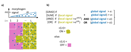
Figure 1: (a) Sketch of the minimal model. The morphogen signal is represented by blue dots and nearest-neighbor interaction by green triangles. A green cell is in state On and signals this to its direct neighbors, a pink cell is Off, i.e., not signaling. The left boundary at $i=0$ is fixed to Off cells, while the right boundary at $i=L+1$ is fixed to On cells. In perpendicular direction we chose periodic boundary conditions. For example, the green cell highlighted by a dark gray frame senses the local signal from its upper, lower, left and right neighbor (light gray frames) canceling to one Off state plus local noise as well as a morphogen concentration of $2m$ plus global noise. (b) Summary of the three rules: [SUM]: Given a cell at position $i$ at time $t$ in state $c(i,t)$: If the local signal subject to Gaussian noise plus the global signal subject to independent Gaussian noise exceeds a global threshold $a$, then the cell state $c$ at the next time step $t+1$ is On, else Off. [AND/OR]: If the local signal exceeds a local threshold AND/OR, then the global signal exceeds the global signal, $c(i,t+1)=$ On.

II Model and observables

Our theoretical approach is based on a minimal model for the formation of a gene expression boundary in a single layer of cells. The model focuses on the interplay between a morphogen gradient and local cell-cell signaling. Consequently, it ignores all other processes occurring in developmental systems that might change the neighborhood relation of cells, such as cell migration, proliferation, cell death, and cell shape changes. Also, we treat the local coupling between cells completely on the level of information and do not consider additional physical mechanisms, such as differential cell adhesion and differential mechanical tension [1]. The role of the morphogen gradient is to activate the target gene in cells at positions where the morphogen level exceeds a threshold, thereby creating a gene expression boundary. By contrast, the local signaling provides a means for cells to exchange information about their gene expression state with their neighbors and to use this information to modulate their response to the morphogen gradient.

Our model and the relevant observables are described in detail in the following two subsections. On a conceptual level, it may be helpful to think of the model as a two-dimensional (2D) kinetic Ising model, which has unusual couplings between neighboring spins and is subject to an inhomogeneous external magnetic field, see the supplementary material for a detailed comparison [22]. However, in the context of our study it is important that there are different sources of noise, not just a single thermal noise. First, there is noise from the global morphogen signal. In developmental systems, all processes involving the morphogen — morphogen production, morphogen transport, morphogen uptake, and signaling — contribute to this noise. For example, morphogen production is subject to stochastic variations in morphogen molecule synthesis and secretion [9, 23], morphogen transport by diffusion is a stochastic process itself and can moreover be hindered by barriers [24]. At the morphogen uptake stage, cell-cell variability in the number of receptors, binding of molecules to receptors and receptor occupancy are additional sources of noise [25, 10, 9]. Finally, activation of the signaling pathways and gene regulation are also noisy processes [23]. These latter processes are also the cause for noise in cell-cell signaling.

Model

We consider a square grid of $L\times L$ cells, see Fig. 1. The state of a cell is reduced to either ‘On’ or ‘Off’, $c=+\frac{1}{2}\text{ or }-\frac{1}{2}$. Along the axis of the gradient (index $i$) the boundary conditions of our grid are fixed to Off on the left ($i=0$) and On on the right side of the grid ($i=L$). In the perpendicular direction (index $j$) we apply periodic boundary conditions. The cell state is updated according to a signal processing rule $\mathcal{L}$, which we also refer to as signal integration rule. The state can change at discrete time steps. The rule processes two different signals: the global signal at the cells position $(i,j)$, $s^{G}_{ij}(t)$, representing the morphogen gradient, and a local signal, $s^{L}_{ij}(t)$, encoding the state of the cells within $c_{ij}$’s neighborhood,

$$c_{ij}(t+1)=\mathcal{L}\left[s^{G}_{ij}(t),\>s^{L}_{ij}(t)\right]\>.$$ (1)

A Boolean logic is the common simplification of the biologically observed Hill type regulation, as the sigmoidal form becomes a sharp threshold in the limit of large Hill coefficients [26].

Global signal

The stochastic global signal at a cell with index $(i,j)$ is given as

$$s^{G}_{ij}(t)=m\>i+\xi_{ij}^{G}(t)\>,$$ (2)

with $m$, $m\in[0,1]\subset\mathbb{R},$ the morphogen gradient slope at $i$ and $\xi^{G}$ additive Gaussian white noise with mean zero and standard deviation $\sigma^{G}$.

During embryogenesis, morphogen molecule concentration is commonly assumed to be exponentially decaying within the tissue. Inspired by Ref. [19], we interpret the logarithm of the molecule concentration as the actual signal (Weber-Fechner law), resulting in a linear morphogen gradient signal.

French Flag mechanism

We refer to a signal processing rule that only depends on the global signal and compares it to a global threshold $a$ as pure gradient rule $\mathcal{L}^{\text{GRAD}}\left[s^{G}\right]$. It is the analog of the French Flag mechanism [3]. More precisely

$$\mathcal{L}^{\text{GRAD}}\left[s^{G}_{ij}(t)\right] :=\Theta\left[s^{G}_{ij}(t)-a\right]-\frac{1}{2}\>,$$ (3)

with $\Theta$ denoting the Heaviside step function with convention $\Theta\left[0\right]=0$. The state of a cell at position $i$ at $t+1$ is $+\frac{1}{2}$ if the global signal exceeds the global threshold $a$ and $-\frac{1}{2}$ else.

Local signal

The signal processing rules with correction ability additionally make use of a local signal $s^{L}$ that stems from nearest-neighbor cells communicating their state. We conservatively assume that the central cell cannot sense from which neighbor the signal came from and thus define $s^{L}$ to be the sum of these signals

$$s^{L}_{ij}(t)=\sum\limits_{(k,l)\>\in\>\text{neighbors}(i,j)}c_{kl}(t)\quad+\xi_{ij}^{L}(t)\>.$$ (4)

‘neighbors’ refers to the upper, lower, left and right neighbor (von Neumann’s neighborhood). $\xi^{L}$ is chosen to be Gaussian white noise with a mean of zero and standard deviation $\sigma^{L}$. Consequently, the noise realization is in $\mathbb{R}$, and with that the local signal.

Correction mechanisms

To implement a correction mechanism, each cell needs to combine the two noisy signals $s^{L}$ and $s^{G}$. It is by no means clear how this combination is optimally performed. Straight forwardly, we can add up both signals and compare the result to the global threshold $a$. We will refer to this procedure as SUM rule $\mathcal{L}^{\text{SUM}}$,

$$\mathcal{L}^{\text{SUM}}\left[s^{L}_{ij}(t),s^{G}_{ij}(t)\right]=\Theta\left[s^{L}_{ij}(t)+s^{G}_{ij}(t)-a\right]-\frac{1}{2}\>.$$ (5)

Note that the contribution of the local signal to the full signal can take any value by rescaling $m$ and $a$ simultaneously.
Alternatively, both signals could be processed separately and the results combined by an AND or OR rule, denoted by $\mathcal{L}^{\text{AND}}$ and $\mathcal{L}^{\text{OR}}$, respectively. A NOR or XOR rule is not expected to perform well in our setting, as both signals are chosen to promote the On state, see also Appendix A for a more explicit discussion. Processing the local signal separately requires an additional threshold, $a^{\text{AND}}$ respectively $a^{\text{OR}}$,

$$\mathcal{L}^{\text{AND}}\left[s^{L}_{ij}(t),s^{G}_{ij}(t)\right] =\Theta\left[s^{L}_{ij}(t)-a^{\text{AND}}\right]\Theta\left[s^{G}_{ij}(t)-a\right]-\frac{1}{2}\>,$$

$$\mathcal{L}^{\text{OR}}\left[s^{L}_{ij}(t),s^{G}_{ij}(t)\right] =\Theta\left[s^{L}_{ij}(t)-a^{\text{OR}}\right]+\Theta\left[s^{G}_{ij}(t)-a\right]$$

$$\>-\Theta\left[s^{L}_{ij}(t)-a^{\text{OR}}\right]\Theta\left[s^{G}_{ij}(t)-a\right]-\frac{1}{2}\>.$$

If we want the AND and the OR rule to be able to produce a boundary from an arbitrary initial grid for all noise levels, equivalently to the pure gradient mechanism, then we find that there is only one choice for the local thresholds, i.e., $a^{\text{AND}}=-1$ and $a^{\text{OR}}=+1$. For larger $a^{\text{AND}}$ values the AND rule cannot exit an initial all Off grid in the small noise scenario. On the other hand, smaller $a^{\text{AND}}$ values increase the fuzziness as they reduce the correction ability of the AND rule, as for $a^{\text{AND}}\ll-1$ we essentially have a pure gradient rule. A quantitative version of this argument and numeric confirmation are shown in Appendix B. Equivalent reasoning holds true for the OR rule when starting from an all On grid.

For a choice of local thresholds such that $a^{\text{AND}}=-a^{\text{OR}}$ we observe in simulations and can show, a direct ‘particle-hole’ correspondence between the AND and the OR rule, resulting in

$$\langle c_{ij}^{\text{AND}}\rangle\approx-\langle c_{\tilde{i}j}^{\text{OR}}\rangle,\quad\text{with}\quad\tilde{i}=2\frac{a}{m}-i\>,$$ (6)

with the approximate relation becoming exact in the limit of an infinite grid. The approximation generally works well for a boundary position that is distant from the grid boundary. Essentially, this relation follows because the local signal is antisymmetric with respect to exchanging On for Off states and linearity of the global signal, as made explicit in Appendix C.

These rules can also be motivated by common input functions to gene transcription [21, 20, 26]: Either both signals or their products within the signal processing pathway can occupy the same promoter, a regulation scheme modeled by the SUM rule, motivated by Ref. [27]. Or there is a different promoter for each signal such that either both have to be occupied to switch on gene transcription, representing the AND rule, or occupation of one is sufficient implying an OR rule. The global threshold $a$ thereby corresponds to the binding affinity of the transcription factor stemming from the morphogen signal to its promoter and the local thresholds to the binding affinity of the transcription factor related to the local direct neighbor signaling. However, the model is not limited to regulation of a cell’s transcriptional state by chemical signaling. It also applies to bioelectrical signaling during embryogenesis for patterning processes involving a long ranged electric gradient, where cell-cell signaling is performed via ion channels and gap junctions [13], for instance. Or to mechanical cues as long as the cell neighborhoods are not altered.

Transforming and reducing the parameter set

The parameters characterizing the model are the grid length $L$, morphogen gradient slope $m$, global threshold $a$, and the standard deviations of the global and local noise $\sigma^{G}$ and $\sigma^{L}$. In order to arrive at a description in more natural parameters, we transform $m,\>a$ to $m,\>\frac{a}{m}$ as $\frac{a}{m}$ corresponds to the spatial position where the morphogen signal equals its global threshold. Also, we transform the independent noises to a total noise and the relative contributions. The total noise is defined as $\xi:=\xi^{L}+\xi^{G}$ with standard deviation $\sigma$ and local to total noise ratio $\alpha$ defined as

$$\sigma^{2}:=\left(\sigma^{G}\right)^{2}+\left(\sigma^{L}\right)^{2},\quad\text{and }\alpha:=\frac{\left(\sigma^{L}\right)^{2}}{\sigma^{2}}\>.$$ (7)

If not stated otherwise, then we set the local to total noise ratio $\alpha$ to $\alpha=\frac{2}{mL+2}$ as 2 is the maximal deterministic local signal and $mL$ the maximal global signal.

Simulation scheme

For simplicity and computational efficiency, we chose the dynamics to consist of synchronous updates of the complete grid at equidistant, discrete time steps. We checked that the stationary state results qualitatively agree with a random update of all grid cells for the boundary position and fuzziness, see the supplementary material [22].

Observables

We are interested in a correctly positioned boundary between different cell types that is straight and sharp. To make these notions quantitative, we define the boundary position $\mathcal{B}(t)$ of a grid at time $t$ to be the average number of cells in Off state, per row,

$$\mathcal{B}(t):=\frac{1}{L}\sum\limits_{i,j}\delta\left(c_{ij},-\frac{1}{2}\right)\>,$$ (8)

with $\delta$ the Kronecker delta. This definition is related to the magnetization in Ising models and circumvents problems of other measures as discussed in the supplementary material [22].

The fuzziness $\mathcal{F}(t)$ of a grid at time $t$ is then defined as the number of sites in the wrong state with respect to the boundary position, rounded to its closest integer, in percentage of the total number of cells,

$$\mathcal{F}(t):=\frac{1}{L^{2}}\left(\sum\limits_{i<\mathcal{B},j}\delta\left(c_{ij},\frac{1}{2}\right)+\sum\limits_{i>\mathcal{B},j}\delta\left(c_{ij},-\frac{1}{2}\right)\right)\>.$$ (9)

Note that this definition combines two notions characterizing the quality of a boundary, its roughness and its softness. Given a unique boundary line, i.e., a grid configuration without holes, the roughness quantifies the boundaries’ deviation from a straight line. In case of frequent holes, the softness measures the width of the holey region that constitutes the boundary. In the system presented here, holes do occur, but are rare, and thus we do not account for them separately. The chosen definition of boundary fuzziness counts both types of boundary errors equivalently. Exemplary grids visualizing boundary position and fuzziness can be found in the supplementary material [22]. The ensemble averages of the boundary position $\left\langle\mathcal{B}\right\rangle$ and the fuzziness $\left\langle\mathcal{F}\right\rangle$ are approximated by their time averages in the stationary state.

III Results

For a boundary established by a global signal in the form of a gradient with slope $m$ and local signaling between neighboring cells, we want to measure the dependence of the boundary position $\mathcal{B}$ and its fuzziness $\mathcal{F}$ on the total noise. The total noise with standard deviation $\sigma$ sums independent Gaussian noise on the global and the local signal.

III.1 Kinetics of approaching the stationary state

We start our investigation of the correction mechanisms SUM, AND and OR by studying the boundary position $\mathcal{B}(t)$ and fuzziness $\mathcal{F}(t)$ as a function of time using a synchronous update scheme of the whole grid. Toward that end, we consider an arbitrary but fixed threshold $a$, morphogen slope $m$, and grid length $L$, here chosen such that the boundary position of the pure gradient mechanism is in the middle of the grid.

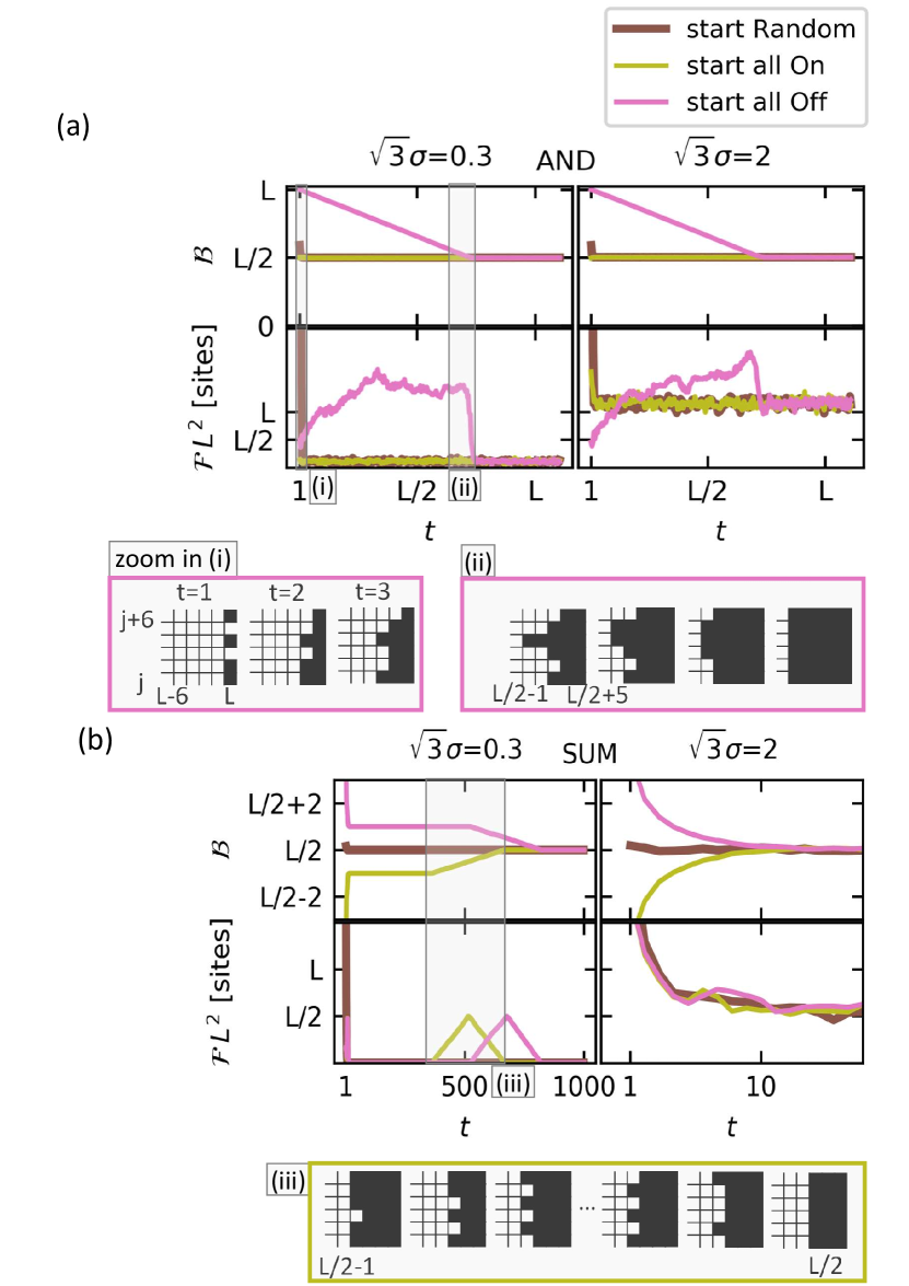
Figure 2: Exemplary boundary position $\mathcal{B}$ and fuzziness $\mathcal{F}$ (in terms of number of wrong cells) time traces starting from different initial conditions at $t=0$, depicted in different colors, for the AND rule in the upper panel (a) and the SUM rule in the lower panel (b) subject to a small (first column) and a large (second column) noise value. Note that for the AND rule time is measured in terms of grid length. The grid length $L=255$ is odd and $a=64.5$ and $m=0.5$ are chosen such that the stable boundary is in the grid center, only $t\geq 1$ are shown for better visibility. Inserts (i)-(iii) provide a zoom in of 6$\times$6 sites to the grid, for few time steps. For the AND rule, starting from an all Off initial grid, zoom in (i) sketches the first three time steps, while zoom in (ii) provides a potential time trace of reaching the stable boundary position, which is $L/2$ here. For the SUM rule, zoom in (iii) sketches boundary destabilization and transition to a straight and sharp boundary.

AND and OR rule

We characterize the evolution under the AND rule, plotted in Fig. 2(a) for three different initial conditions: a random initial grid, a grid of all cells in state Off (‘all Off’), and a grid of all cells in state On (‘all On’). The first column shows for an exemplary low noise level the boundary position in the first row and the fuzziness in the second row in dependence of time.

Starting from an all Off grid the boundary position $\mathcal{B}$ moves roughly one cell per time step until it reaches its stationary value [see Fig. 2(a), first row]. The fuzziness $\mathcal{F}$ increases until it drops sharply when the stationary boundary position has been reached. Note that already for low noise the fuzziness time trace remains wiggly for all times, implying that the stationary boundary is fuzzy. Remarkably, for larger noise the boundary position moves at the same rate. Only the stationary boundary is more fuzzy compared to the boundary in the low noise regime [see right column of Fig. 2(a)]. Consequently, the transition time to the initial condition independent, stationary, boundary position does not depend on the noise level. We also observe that the transition time is on the order of magnitude of the stationary boundary position. The last row of Fig. 3 confirms this independence more generally.
An intuitive picture, explained in more detail in the supplementary material [22], for the dynamics is the following: By definition, the AND rule only allows cells to switch on if they have at least one On neighbor and the gradient signal exceeds its threshold $a$. The second condition is satisfied for all cells to the right of position $i=\left\lfloor\frac{a}{m}\right\rfloor$ by the deterministic part of the gradient signal. When starting from an all Off grid, the first condition implies that only cells at the right boundary can switch on due to cells at $i=L+1$ being On (fixed grid-boundary condition choice). Each boundary cell can move at most one cell forward per time step [see Figs. 2(i) and (ii)]. Quantitatively, a cell with exactly one On neighbor switches on with probability 1/2 independent of the total noise level. A cell with more than one On neighbor switches on with a probability close to 1. Note that our choice of grid-boundary conditions, $c_{0,j}=0$ and $c_{L+1,j}=1$ for all rows $j$, does not substantially simplify the patterning task for the rules. The AND rule (and also the OR and SUM rule as we will see later) cannot just shift the sharp cell state boundary at $L$ to its stationary position. Even if we had only one cell in On state at $i=L+1$ the rules could still establish a boundary at the center of the grid. However, this choice of grid boundary would artificially destabilize the correct stationary pattern due to local signaling, as the correct pattern requires that cells at $i=L$ are On.
For the ‘all On’ initial grid, convergence to the stationary boundary position occurs within the first time step, as the deterministic part of the neighborhood signal exceeds $a^{\text{AND}}=-1$ everywhere in the grid and the AND rule essentially reduces to the pure gradient mechanism. For a random initial grid, at $t=0$, the neighborhood signal exceeds $a^{\text{AND}}$ for about 3/4th of the cells in each column, thus convergence is fast, as well.

The OR rule by definition can only switch off one cell width at a time when starting from an initial grid of On cells. Consequently, the time traces of the OR rule qualitatively correspond to the ones of the AND rule with On-Off inverted initial conditions, see Fig. 9 in the Appendix. This was to be expected from the AND-OR relationship, Eq. (6).

SUM rule

Figure 2(b) shows evolution under the SUM rule and exhibits qualitatively different dynamics. The right column shows the large noise regime. We see that already within 20 time steps the different boundary position traces have converged. We also note that the boundary is fuzzy in contrast to the low noise regime. For a low noise level, as depicted in the left column of Fig. 2(b), the dynamics is more complex. While for all initial conditions, the boundary quickly reaches a position close to its stationary value, full convergence is very slow. Thus, in contrast to the AND and OR rule the transition time strongly depends on the noise level. Starting from any initial condition, the boundary reaches a position close to its stationary value within few time steps. Movement toward its final position happens when noise induces a seed at the boundary linearly spreading until all cells within the same column have switched state. As sketched in Fig. 2(iii), one seed induces a switch of both of its neighbors in the next time step and so forth until the complete column of former boundary cells has switched state, in case of an odd grid height. Then the boundary remains straight until the next seed occurs. In case of an even grid length, the pattern with every second boundary cell switched on corresponds to a metastable state, see Appendix D. The waiting time distribution for the next seed to destabilize the metastable boundary is strongly noise level dependent. In fact, the transition time until the stationary state at $\left\lfloor\frac{a}{m}\right\rfloor$ is reached can be approximated by

$$\mathcal{T}(\sigma)\approx\frac{12}{L}\exp\left(\frac{\sqrt{3}}{2\sigma^{2}}\right)$$ (10)

for sufficiently small $\sigma$, as shown in the supplementary material [22], and plotted in Fig. 3. This functional form clearly shows the nonlinear dependence of the transition time on the noise level. As expected, the transition time is inversely proportional to the system length as a seed is more likely the more sites in the column next to the boundary noise is acting on.

III.2 Characterizing the stationary state’s dependence on the noise level

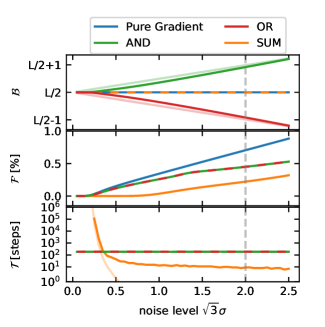
Figure 3: Overview of different stationary state behavior of the pure gradient, SUM, AND, and OR rule depending on noise level regime, exemplary for $L=256,\>a=64.5,\>m=0.5$. On the $x$-axis, we use noise level $\sqrt{3}\sigma$ instead of $\sigma$ for better intuition of the strength of the total noise: More than $90\%$ of all noise realizations are within the interval $\left[-\sqrt{3}\sigma,+\sqrt{3}\sigma\right]$. Also, a uniform distribution within $\left[-\sqrt{3}\sigma,+\sqrt{3}\sigma\right]$ has variance $\sigma^{2}$. In the first row, the time-averaged boundary position $\mathcal{B}$ for each rule is shown, where dashes indicate that the lines overlap. The light green and red lines show the analytical estimate of the boundary position for the AND and OR rule. In the second row, time-averaged fuzziness $\mathcal{F}$ in $\%$ of the total number of grid sites is plotted. The last row shows the transition time $\mathcal{T}$ until the initial condition independent state was reached, where a value of $10^{6}$ implies that it has not converged within the simulation time. The light yellow line depicts the $\mathcal{T}$ approximation for the SUM rule for small noise levels, see Eq. (10).

Figure 3 shows the characteristic stationary state properties of the three correction mechanisms SUM, AND, and OR as a function of the total noises’ standard deviation $\sigma$ for an exemplary threshold $a$ and morphogen signal slope $m$ choice. For direct comparison, the results without correction mechanism (pure gradient) are plotted in blue. Each row shows a different observable — the time-averaged boundary position $\mathcal{B}$, fuzziness $\mathcal{F}$, and, in the last column, the transition time $\mathcal{T}$. For simplicity, we here use the maximal number of time steps until reaching the stationary state from an all On and an all Off grid as a measure of $\mathcal{T}$. We will discuss the different phenomenologies starting from low noise levels and ending with large noise levels.

Small noise levels

In the last row of Fig. 3 we observe that the SUM rule results have not converged to stationary state within the simulation time of $10^{6}$ time steps in the regime of very low noise levels. This is expected from the previous transition time discussion. Loosely speaking, noise is needed to forget the initial grid state. In contrast, the AND and OR rule’s transition time $\mathcal{T}$ scales linearly with the boundary position, irrespective of the noise level as discussed in Sec. III.1. The transition time from a particular initial condition, e.g., ‘all On’, can be significantly smaller, see Fig. 2. Turning to the second row of Fig. 3, we note that the boundary fuzziness for the SUM rule is remarkably close to zero for small yet sufficiently large noise levels to allow for convergence of the SUM rule pattern. An effectively nonfuzzy regime is not observed for other rules. In the first row, we observe that the SUM’s boundary position agrees well with the pure gradient rules’ for zero noise, while the AND and OR rules’ boundary position slightly deviate up to a cell width. Indeed, we can derive analytic approximations for the stationary boundary positions, as outlined below, and refer to Appendix E for further details. For the SUM rule, the stationary boundary position is given by

$$i_{c}^{\text{SUM}}=\left\lfloor\frac{a}{m}\right\rfloor=i_{c}^{\text{Grad}}\>,$$ (11)

with $\left\lfloor\cdot\right\rfloor$ denoting the floor operator. Consequently, the stationary boundary will scale with system size in the same way as for the pure gradient rule for zero noise. The stationary boundary position of the AND rule includes an additional term linear in the noise level,

$$i_{c}^{\text{AND}}\approx\left\lfloor\frac{a}{m}\right\rfloor+0.25\frac{\sqrt{3}\sigma}{m}\sqrt{1-\frac{2}{2+mL}}\>.$$ (12)

We see that $i_{c}^{\text{AND}}\approx i_{c}^{\text{Grad}}+\frac{\sqrt{3}\sigma}{4m}$ for $mL\gg 2$ which agrees well with simulation results shown in Fig. 3.
For the OR rule, it follows

$$i_{c}^{\text{OR}}\approx\left\lfloor\frac{a}{m}\right\rfloor-0.25\frac{\sqrt{3}\sigma}{m}\sqrt{1-\frac{2}{2+mL}}\>,$$ (13)

by the AND-OR equivalence established in Eq. 6. To derive those expressions for the stationary boundary positions, we started from the following observation: The probability for a defect to disturb the boundary at $i_{c}$ needs to be smaller than the one for a potential boundary one cell width to its left, at $i_{c-1}$, or to its right, at $i_{c+1}$. Those disturbances can be either an Off cell right of the boundary (Off-in-On defect) or an On cell left of the boundary (On-in-Off defect). For a sketch of an Off-in-On defect, see the first grid of Fig. 2(iii). Consequently, two conditions need to be satisfied such that the stationary boundary position is at cell index $i=i_{c}$. To the left, the probability to destabilize a boundary at $i_{c}-1$ by an Off-in-On defect has to be smaller or equal to the probability destabilizing a boundary at $i_{c}$ by an On-in-Off defect. To the right, the probability to destabilize a boundary at $i_{c}$ by an On-in-Off defect has to be smaller or equal to the probability destabilizing a boundary at $i_{c}+1$ by an Off-in-On defect. Solving these inequalities with probabilities approximated for the different rules yields the stationary boundary position; see Appendix E. From this calculation we can also see that the probabilities for an On-in-Off defect and an Off-in-On defect at $i_{c}$ depend only on $m$ and $\frac{a}{m}-\left\lfloor\frac{a}{m}\right\rfloor$. These findings suggest that the fuzziness in stationary state only depends on the deviation of $\frac{a}{m}$ to the next integer value. This is also confirmed by numeric results. Intuitively, the morphogen changes at the same rate everywhere in the system and the local interaction is independent of the position per definition.

Intermediate noise levels

For larger noise levels the AND and the OR rule qualitatively exhibit the same behavior as for low noise, in contrast to the SUM rule. In the second row of Fig. 3 we observe a rapid increase in fuzziness for the SUM rule. Time-averaged fuzziness seems to arise from alternating between time intervals of a straight, sharp boundary and time intervals with a disturbance, seeded by a single defect cell, that grows and shrinks for some time before it decays. The probability for a seed is highly nonlinearly, but smoothly, increasing with noise level [22].

Large noise levels

In the regime of large noise we see in the second row in Fig. 3 that the SUM rule yields a less fuzzy boundary than the AND and OR rule, which behave similarly. Indeed, all correction mechanisms outperform the pure gradient rule. We will show that this result is robust for all $a$, $m$ parameter combinations determining the three rules in Sec. III.4, for all grid lengths (Sec. III.3) and for a surprisingly large range of local to total noise ratios $\alpha$ (Sec. III.5).

The boundary position $\mathcal{B}$ resulting from the SUM rule agrees well with the boundary position from the pure gradient as analytically deduced in Appendix E. Although the boundary positions from the AND and OR rules deviate linearly with the standard deviation of the total noise $\sigma$, we will show in Sec. III.3 that both nevertheless scale linearly with system size.

III.3 All rules conserve scaling of the boundary position with system size

In embryogenesis, proportions commonly remain the same irrespective of different embryo or compartment sizes (see [28] for a review). The pure gradient mechanism also exhibits this scaling behavior, provided that the maximal morphogen concentration and the threshold remain constant. In our model these conserved proportions translate to a fixed fraction of On to Off cells within grids of different size for a fixed maximal morphogen signal $mL$. In Fig. 3 we have observed that the stable boundary position formed by the AND and OR rule deviates from the position established by the pure gradient rule. Thus we need to investigate if also the AND and OR rule ensure this property, just with a different fraction. For an exemplary parameter set, $a=2,\>mL=8$ at a large noise level $\sqrt{3}\sigma=2$, we can see in Fig. 4 that this is indeed the case. The reason that AND (OR) rules’ boundary position tends to larger (smaller) $\mathcal{B}$ values is that it discourages (encourages) On cells. As the slope $m$ becomes smaller and smaller ($mL$ fixed) the regime around the boundary in which this effect plays a role increases linearly with system length. This leads to a constant boundary position $\mathcal{B}$ over grid length $L$ ratio. The deviation of this value from the pure gradient rules’ result can be approximated by Eq. (12) and Eq. (13), respectively. For small grid sizes, we see that the relative boundary position of any rule has not yet converged to its large grid limit. The reason is of technical nature: Our parameter choices imply that defect cells at the left of the boundary are more common than at its right, see Appendix F for a more detailed argument.

Figure 4 shows that the fraction of sites in the wrong state converges to a stable value for large system lengths. Consequently, the improved boundary sharpness is not only a finite grid size effect. The observation that the SUM rule performs best, the AND and OR rule not as well, but better than pure gradient, also holds true for all tested grid lengths.

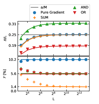
Figure 4: Upper panel: Relative time-averaged boundary position $\mathcal{B}$ for all three rules and pure gradient for increasing grid lengths $L$ for a fixed noise level of $\sqrt{3}\sigma=2$, $a=2,\>mL=8,$ and all Off initial grid. Bottom panel: Time-averaged boundary fuzziness $\mathcal{F}$ in percentage of the number of cells in the grid. For sufficiently large grids the relative fuzziness converges to a constant value that is smallest for the SUM rule, larger for the AND and OR rule and highest for the pure gradient rule.

III.4 Systematic exploration of the parameter space

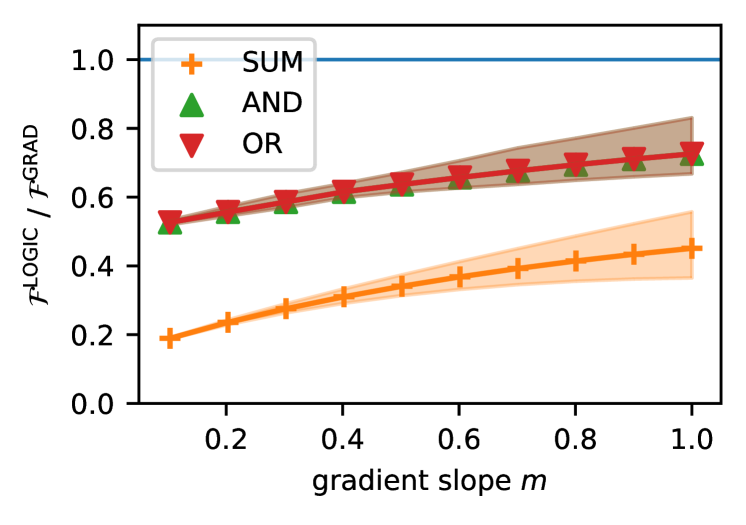
Figure 5: For a fixed noise level $\sqrt{3}\sigma=2$ and grid length $L=256$ the fuzziness $\mathcal{F}$ fraction of the boundary formed by a correction rule (SUM, AND, OR) and the boundary fuzziness due to pure gradient is shown in dependence of the gradient slope $m$. Single markers correspond to the average fuzziness fraction over all $a$ values and are interpolated by a solid line. The shaded area is restricted by the interpolation of the minimal (lower edge) and maximal (upper edge) fuzziness fraction with respect to all threshold $a$ values.

We want to know how much smoother the boundary established by the correction mechanisms is compared to the boundary established by the pure gradient rule. Until now, we have shown results for isolated points in the parameter space. Now we want to study the whole parameter space spanned by threshold $a$ and morphogen signal slope $m$. It is equivalent to varying $m$ and $\frac{a}{m}$ from $\left\lfloor\frac{a}{m}\right\rfloor$ to $\left\lceil\frac{a}{m}\right\rceil$ as discussed in Sec. III.2.
Let us fix a high noise level, $\sqrt{3}\sigma=2$. We measure the boundary smoothing capability of a correction rule in terms of the ratio of the boundary fuzziness resulting from a correction mechanism to the boundary fuzziness caused by the pure gradient rule, $\mathcal{F}^{\text{LOGIC}}(\sqrt{3}\sigma=2)/\mathcal{F}^{\text{GRAD}}(\sqrt{3}\sigma=2)$. In order to show the full range of fuzziness ratios caused by varying $a$ and $m$ in Fig. 5, we choose for each $m$ to display the ratios’ minimal and maximal value for any $a$ (interpolated by the lower and upper edge of the shaded area), as well as the ratios’ average over $a$ (data points interpolated by sold line).

We observe that $\mathcal{F}$ ratios are below one and that the SUM ratio is smallest for all morphogen slopes $m$. This implies that all three rules perform better for every threshold $a$ and gradient slope $m$ than the pure gradient rule with respect to fuzziness reduction. The performance gap between the pure gradient and the correction rules is smaller for larger morphogen slopes, and thus the most conservative choice for $m$ is $m=1.0$. Intuitively, this is because the steepest gradient provides the largest signal differences between neighboring cells in $i$ direction.

III.5 Variation of local to total noise ratio

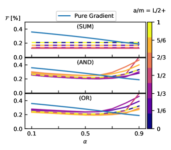
Figure 6: Fuzziness $\mathcal{F}$ at $\sqrt{3}\sigma=2$ in dependence of the local to total noise variance, $\alpha$ for $m=1.0$, one row for each correction mechanism. The blue line depicts the pure gradient performance, while the differently colored lines correspond to the correction mechanism result for different $a$/$m$ combinations, $L=256$.

The magnitude and ratio of local to global noise representing a variety of different processes as mentioned in the Introduction is not known. Still, for a fixed maximum morphogen signal $mL$, we have only considered one particular ratio of the local noise $\xi^{L}$ to total noise $\xi^{L}+\xi^{G}$ ratio $\alpha$, $\alpha=\frac{(\sigma^{L})^{2}}{(\sigma^{L})^{2}+(\sigma^{G})^{2}}=\frac{2}{2+mL}$ so far. Intuitively, the pure gradient rule should perform better than the correction mechanisms for large $\alpha$. By definition, the pure gradient rule only experiences noise on the global signal, which approaches zero for the local to total noise ratio $\alpha$ approaching 1. The correction mechanisms, however, process an additional highly error-prone signal, the local signal. To test this intuition, we vary the local to total noise ratio $\alpha$ between 0.1 and 0.9, see Fig. 6 for all different $\frac{a}{m}$ combinations with $m=1.0$, depicted in different colors. The maximal slope $m=1.0$ is chosen to ensure the best relative pure gradient performance, as discussed in Sec. III.4.

Per definition, the SUM rule (first row) is independent of $\alpha$, as it adds up the Gaussian distributed local $\xi^{L}\sim\mathcal{N}(0,(\sigma^{L})^{2})$ and global noise $\xi^{G}\sim\mathcal{N}(0,(\sigma^{G})^{2})$, yielding $\xi^{L}+\xi^{G}\sim\mathcal{N}(0,\sigma^{2})$. The AND and OR rule perform worse relative to the SUM rule the larger $\alpha$ is. Surprisingly, the $\alpha$ value, where pure gradient (blue line) performs equally well than the correction mechanisms (other colors) is well beyond one half. This implies that a correction mechanism can sharpen the boundary, even if it is subject to more than twice as much noise than the pure gradient rule.

IV Discussion

Precise boundary formation is a remarkable phenomenon in developing systems and aspiring goal in synthetic systems. Here our objective was not to study any specific system, but to systematically explore how different logical couplings of cell-cell communication with a gradient signal can aid boundary formation.

In a minimal model of boundary formation consisting of cells that are either signaling (On) or inactive (Off), we studied three different correction mechanisms using this nearest-neighbor interaction in addition to a global (grid spanning) signal gradient. Those three rules either sum both signals (SUM) and subsequently compare the result to a global threshold $a$ or compare each signal to a local and global threshold separately (AND, OR). Consequently, for a signal processing cell to switch to or maintain an On state, in case of the SUM rule the sum of both signals has to exceed the global threshold. The AND rule requires both signals to exceed their respective thresholds independently, while the OR rule requires only one signal to exceed its threshold. We examined which rule performs best in which regime of total noise, consisting of additive Gaussian noise on the local and the global signal. As motivated in the Introduction, performance is measured in terms of (i) reduction in boundary fuzziness, (ii) short transition time to stationary boundary position, (iii) position tuneable by threshold, and (iv) scaling with system size.

We found that (i) the SUM rule achieves the strongest fuzziness reduction, while the AND and OR rule yield comparably less reduction. Only if the noise on the global signal is much smaller than the noise on the local signal, the pure gradient ensures a sharper separation of cells with different gene expression states. (ii) However, transition to stationary state takes more time for any correction mechanism than for the pure gradient rule, which establishes the stationary boundary within one time step. The SUM rule generates a boundary position that deviates by few sites within one time step for sufficiently steep morphogen slopes. Exact convergence strongly depends on the noise level — the smaller, the slower. Qualitatively different, convergence of the AND and OR rule does not depend on the noise level, but on the initial state of the grid. In the best case it happens within one time step, in the worst case in order of grid length $L$ time steps. A short transition time is desirable in development, as boundary cells often act at organizing cells for the next patterning process [1]. Also, fast morphogenesis is favorable to protect against predators. (iii) The boundary position can be tuned by changing the global threshold value $a$ in a similar manner than for the pure gradient mechanism. This programability is of biological significance, as the threshold $a$ was motivated by the binding affinity of the signals’ transcription factor to the promoter of the gene, that is switched on. Possibly, variations of same theme among related species, such as a stripe that differs in width, can be explained as variations of the binding affinity. (iv) For fixed threshold value $a$ and morphogen signal slope $m$ the SUM rule yields the same boundary position as the pure gradient, while the AND and OR rules’ boundary positions deviate by a small amount. Nevertheless, the boundary position established by any rule scales linearly with system size. The scaling property ensures compatibility with the observation that embryos of the same species differ (slightly) in size, but pattern ratios are often conserved [28].

What is the underlying reason that the SUM rule outperforms the AND and OR rule in terms of fuzziness reduction? We believe this is because the SUM rule first averages the involved noises allowing them to cancel, before applying the nonlinearity in the form of comparing to a threshold. The deterministic signal is summed, while the Gaussian noise’s standard deviations only add in quadrature. For the AND and OR rule it is the other way round: They threshold each signal separately before combining the pieces of information. However, there are biological problems where this signal processing scheme — first thresholding, and then combining — is actually optimal, for example in case of a rare signal. Rod cells in the retina specialized to detecting very dim light first threshold before transmitting information to their common bipolar cell, which consecutively sums those digitized signals [29]. If the bipolar cell would first sum the signal of its numerous rod cells, then the simultaneously summed up noise would make it likely for the bipolar cells to confuse total darkness (no photon) with dim light (three or more photons). Consistent with the system presented here, it has been found that only those rod cells specialized for dim light detection process signal by thresholding before summing [30].

In a synthetic setup it is feasible to experimentally test our predictions as all necessary components have already been designed. On the one hand, tuning of local interactions has been successfully realized in multicellular systems, for example, AND-like, OR-like and in between, graded, SUM-like, regulatory behavior in yeast [31]. A remarkably customizable signal processing scheme in the form of a synthetic Notch pathway is presented in Ref. [16], and also reviewed in Ref. [32] among other protein based synthetic circuits in eukaryotic cells. On the other hand, tuneable processing of synthetic gradients has been demonstrated, such as toggle switch processing of a signal gradient in Escherichia coli [17]. A setup close to developmental biology was constructed within Drosophila wing primordia [15]. A combination of a synthetic gradient and a signal processing pathway that can in principle be customized to the rules discussed in this paper is the synthetic GFP morphogen that regulates target gene expression by a synNotch circuit [14].

Remarkably, the study presented in Ref. [15] raises the question of which additional mechanisms are required for sharp boundary formation as the explored setups did not give rise to sharp boundaries [2]. The toolboxes listed above might be able to test whether the three different rules studied in this paper are candidates for the actual boundary correction necessary to ensure the exact results observed in nature. Also, insights about the potential of local signaling as a correction mechanism might find applications in synthetic biology more generally, as boundary and stripe formation are fundamental tasks in patterning and morphogenesis. To better meet such applications, the presented model can be trivially extended to stripe generation by introducing extra thresholds accordingly. It can be further generalized or modified by including more complex rules or smoothing the hard threshold via Hill-type functions, by considering irregular and dynamic cell grids, or by including additional mechanisms such as cell sorting.

Appendix A Other rule functions

SUM, AND, and OR rules are not the only options to process two signals. Others are XOR and PROD, but we can argue that they are not suited for the boundary formation problem as we modeled it.
Let us start from an all Off grid with an XOR logic. In the next time step without noise it would form the correct boundary. In the consecutive update step, all On cells except those at the boundary would switch Off though, as each is subject to a local neighbor signal greater than any (sensible) local threshold value. Consequently the boundary would not be stable.
The product rule PROD in the presence of noise reads
if (global signal(i) +$\xi^{G}$)$\cdot$ (local signal(i,t) + $\xi^{L}$) $>\>a^{2}$:    cell(i, t+1) = On which implies that the noise would be multiplied by the signal. Consequently, we expect this rule to perform poorly in the presence of sufficiently large noise.

Appendix B $a_{\text{local}}$ optimization

We want the AND and OR rules to be able to produce a boundary from an arbitrary initial grid for all noise levels, equivalently to the pure gradient mechanism. Here we show that the initial grids all Off and all On are sufficient to fix the additional local thresholds $a^{\text{AND}}$ and $a^{\text{OR}}$.

Let us consider an all Off initial grid. At the right border, $i=L$, the global signal exceeds the global threshold $a$ (otherwise the pure gradient rule could not form a nontrivial boundary either). For the AND rule to exit the initial condition, we need $a^{\text{AND}}$ to be smaller or equal than the local signal $s^{L}_{ij}(t)=-1+\xi_{ij}^{L}(t)$. Thus, we need $a^{\text{AND}}\leq-1$. Similarly, for an all On initial grid it follows that $a_{l}^{\text{OR}}\geq 1$. The second condition to determine the optimal local threshold comes from demanding that it stabilizes a straight boundary. To this end, consider a straight boundary, implying that the global signal is close to $a$, but with one On cell left of the boundary. For the AND rule, we want $a^{\text{AND}}\geq-1$ in order to switch Off the defect cell. Taken together this suggests choosing $a^{\text{AND}}=-1$. The opposite scenario, one Off cell right of the boundary, yields $a^{\text{AND}}<1$, which is well satisfied by our choice. Equivalent reasoning yields $a^{\text{OR}}=1$.

We confirmed these analytic arguments numerically for an exemplary small and large noise level, see Fig. 8 and Fig. 8. We observe that the fuzziness decreases with increasing $a^{\text{AND}}$ values. In the small noise example, $a^{\text{AND}}=-1$ is the largest $a^{\text{AND}}$ value such that the AND rule forms a nontrivial boundary (i.e., $\frac{\mathcal{B}}{L}\neq 1$ or 0) independent of starting from an all On grid (red line) or an all Off grid (green line). If we drop the initial grid independence condition, e.g., if it suffices that the AND rule only patterns when starting from an all On initial grid, then the optimal choice of $a^{\text{AND}}$ would depend on the magnitude of deviation of boundary position from the one generated by pure gradient rule (dashed gray line) we are willing to accept. This is deviation is particularly pronounced for large noise as shown in Fig. 8. Results for the OR rule are depicted in the right column and findings are analogous.

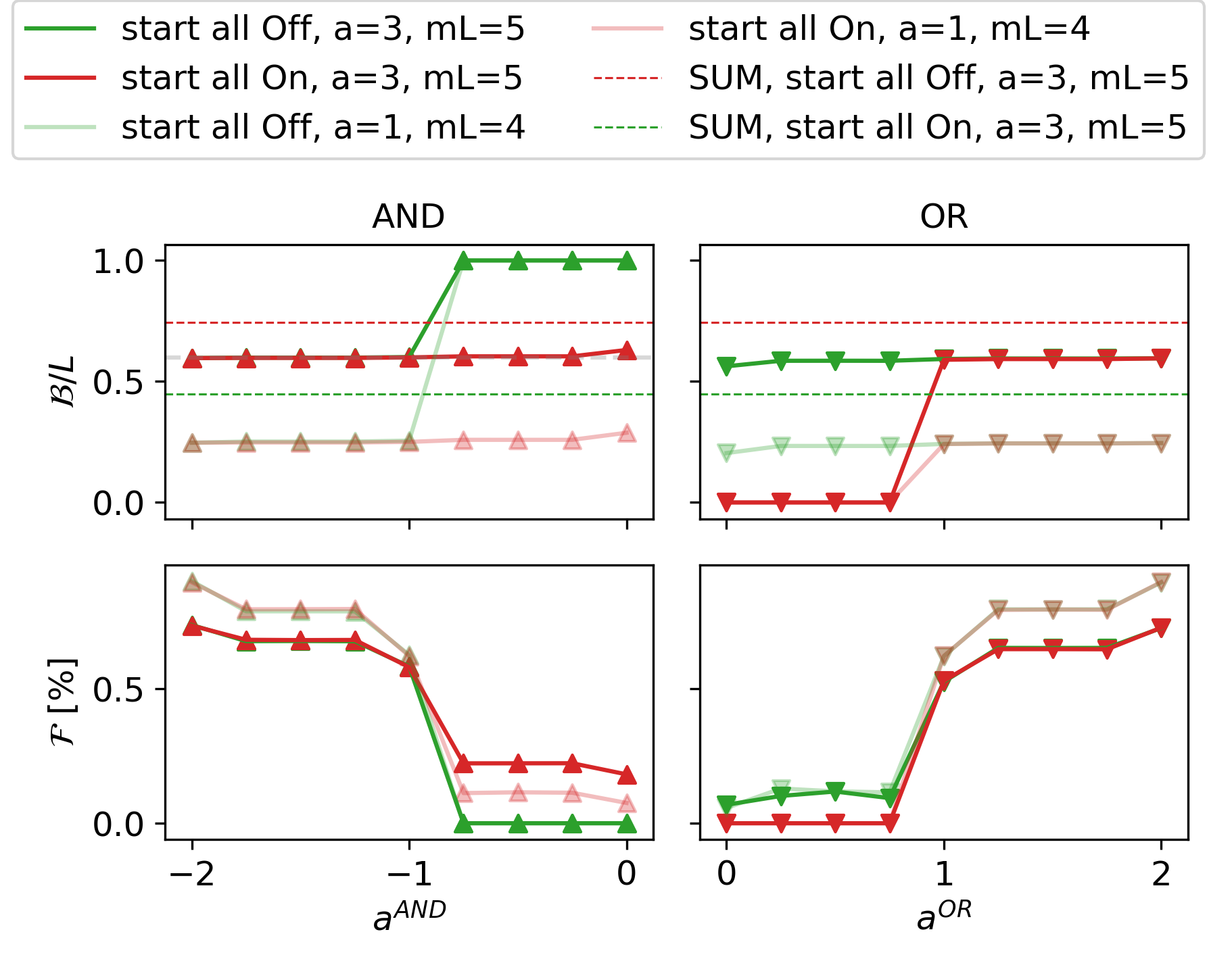
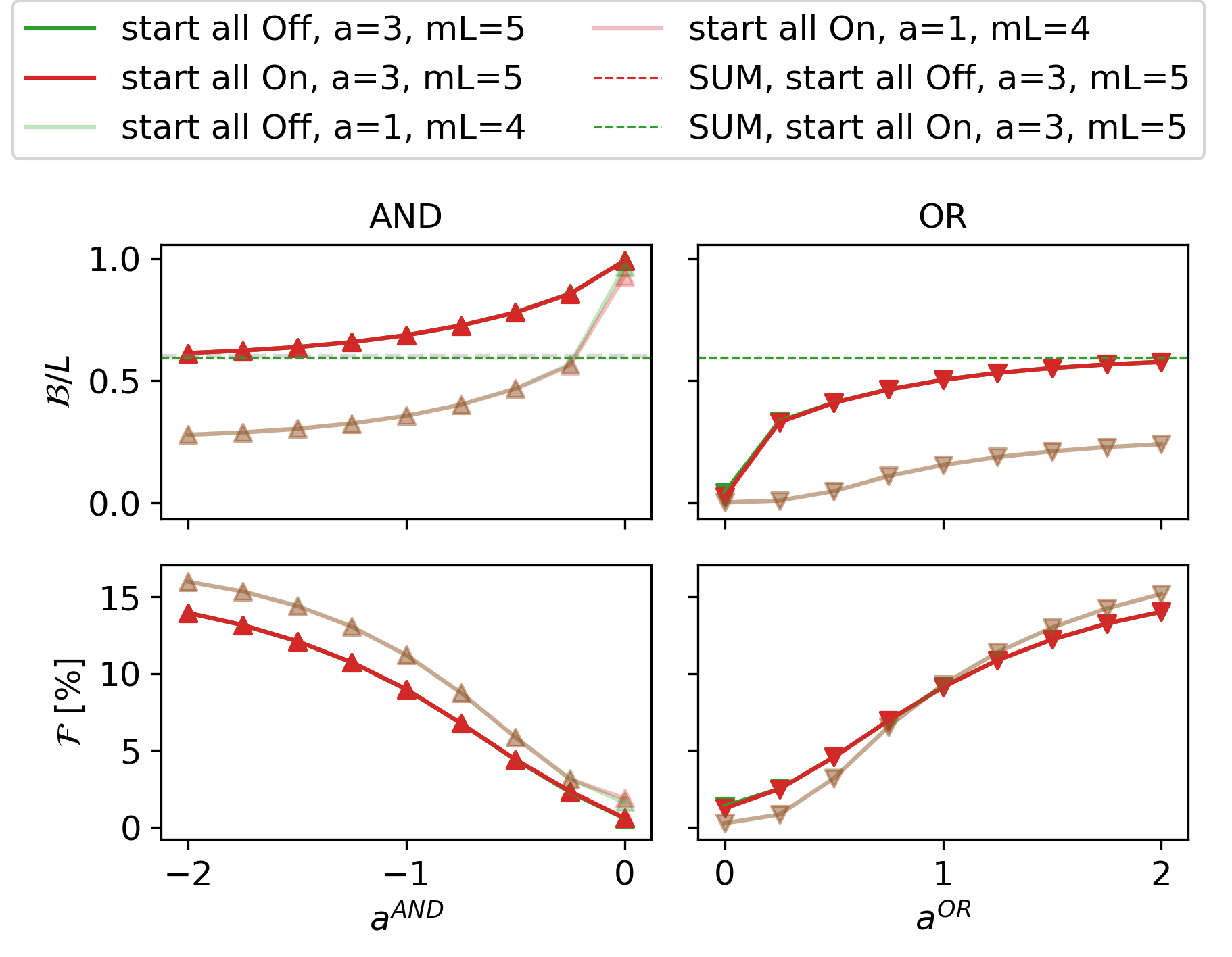
Figure 7: Left column: Relative boundary position $\mathcal{B}/L$ and fuzziness $\mathcal{F}$ with respect to the local threshold $a^{\text{AND}}$ for two different $a$ and $m$ combinations, one plotted full saturation, one light. Green (red) triangles show results for an initial all Off (all On) grid, interpolated by solid lines. The dashed gray line shows the pure gradient $\mathcal{B}/L$. The first column shows that the all Off initial condition can only be exited for $a^{\text{AND}}\leq-1$. The second row shows the fuzziness decrease with increasing $a^{\text{AND}}$. Right column: Analogous results for the OR rule. A small noise level of $0.1=\eta=\sqrt{3}\sigma$ is used.

Figure 8: Same quantities as in Fig. 8 but for a large noise level. Here, both initial conditions yield the same boundary position independent of $a^{\text{AND}}$ choice, but the boundary position deviates strongly from the pure gradient value.

Appendix C Relationship of AND and OR rule for $a^{\text{AND}}=-a^{\text{OR}}$

The choice of $a^{\text{AND}}=-a^{\text{OR}}$ implies close correspondence of the AND and the OR rule in the stationary state. For an infinite grid we have

$$\langle c_{ij}^{\text{AND}}\rangle=-\langle c_{\tilde{i}j}^{\text{OR}}\rangle\quad\text{with}\quad\tilde{i}=2\frac{a}{m}-i\>,$$

where $\langle\rangle$ denotes an ensemble average. Visually speaking $\tilde{i}$ is the mirror reflection of $i$ at the zero transition of the morphogen gradient minus its threshold at $\frac{a}{m}$. For a finite grid, this relation still holds true for parameter combinations $a,\>m$ such that the boundary is distant from edges of the grid. Then we can assume that cells not covered by the $\tilde{i}$ index, which are cells close to the grid boundaries, do not change their state.
We can derive the above relation as follows:

$$c_{i,j}^{\text{AND}} =\mathcal{L}^{\text{AND}}\left(s^{L}_{ij}(t),s^{G}_{ij}(t)\right)$$

$$=\Theta\left(s^{L}_{ij}(t)-a^{\text{AND}}\right)\Theta\left(s^{G}_{ij}(t)-a\right)-\frac{1}{2}\>,$$

whereas

$$-c_{\tilde{i},j}^{\text{OR}} =-\mathcal{L}^{\text{OR}}\left(s^{L}_{\tilde{i}j},s^{G}_{\tilde{i},j}\right)$$

$$=-\left\{1-\left[1-\Theta\left(s^{L}_{ij}(t)-a^{\text{OR}}\right)\right]\right.$$

$$\quad\left.\left[1-\Theta\left(s^{G}_{\tilde{i},j}(t)-a\right)\right]\right\}+\frac{1}{2}$$

$$=\Theta\left(-s^{L}_{ij}(t)+a^{\text{OR}}\right)\Theta\left(-s^{G}_{\tilde{i},j}(t)+a\right)-\frac{1}{2}\>,$$

using that $1-\Theta(x)=\Theta(-x)$.
Now observe that

$$\Theta\left(-s^{G}_{\tilde{i},j}(t)+a\right) =\Theta\left(-s^{G}_{\tilde{i},j}(t)+a\right)$$

$$=\Theta\left(-\tilde{i}m-\xi^{G}_{\tilde{i},j}+a\right)$$

$$=\Theta\left(im-\xi_{ij}^{G}(t)-a\right)\>,$$

where we can neglect the sign change for $\xi_{ij}^{G}(t)$ as it is symmetric around its zero mean. Thus, the contribution by the global signal is by construction of $\tilde{i}$ the same as in the case of the AND rule.
In the stationary state, we have on ensemble average that

$$\left\langle-\sum\limits_{(k,l)\in\mathcal{V}(\tilde{i},j)}c_{k,l}\right\rangle=\left\langle\sum\limits_{(k,l)\in\mathcal{V}(i,j)}c_{k,l}\right\rangle$$ (14)

as the global signal is mirror antisymmetric with respect to the vertical $i=i_{c}$ line and the local signal is independent of the absolute position.
Thus,

$$\left\langle\Theta\left(-s^{L}_{\tilde{i},j}(t)+a^{\text{OR}}\right)\right\rangle$$

$$=\left\langle\Theta\left(-\sum\limits_{(k,l)\in\mathcal{V}(\tilde{i},j)}c_{k,l}-\xi^{L}_{\tilde{i},j}+a^{\text{OR}}\right)\right\rangle$$

$$=\left\langle\Theta\left(\sum\limits_{(k,l)\in\mathcal{V}(i,j)}c_{k,l}+\xi_{ij}^{L}(t)-a^{\text{AND}}\right)\right\rangle\>.$$

Inserting those observations yields the relation Eq. (6). Exemplary time traces from simulation are shown in Fig. 9.

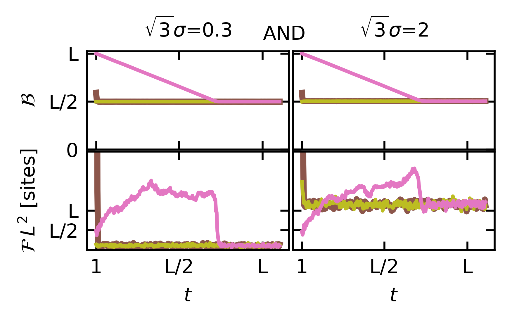
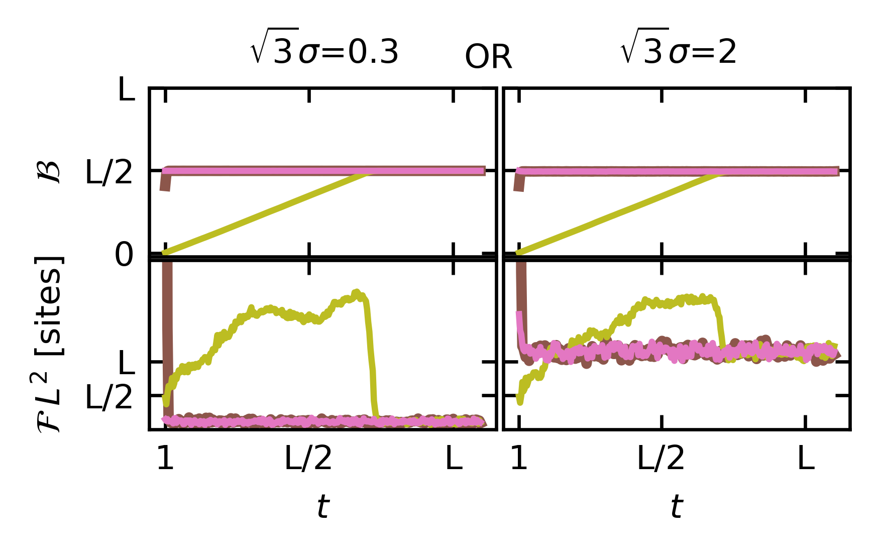
Figure 9: Exemplary time traces from simulation with same parameters as in the main text. For the SUM logic, we observe that the intermediate meta stable state of a half-filled boundary is realized for the boundary transition from $L/2-1$ to $L/2$ (green line).

Appendix D Time traces for even system length

In Fig. 10 we show the time traces of the AND and OR logic as in Fig. 2 of the main text but for an even grid length of $L=256$ instead of the odd $L=255$. An even grid length introduces an additional metastable state for the SUM rule between each subsequent sharp boundaries: the half-filled state, as explained in the main text. For simplicity, we thus chose to show the closest odd state grid in the main text. Here, we display the even $L=256$ version for completeness to show that except for this additional intermediate metastable state nothing changes.

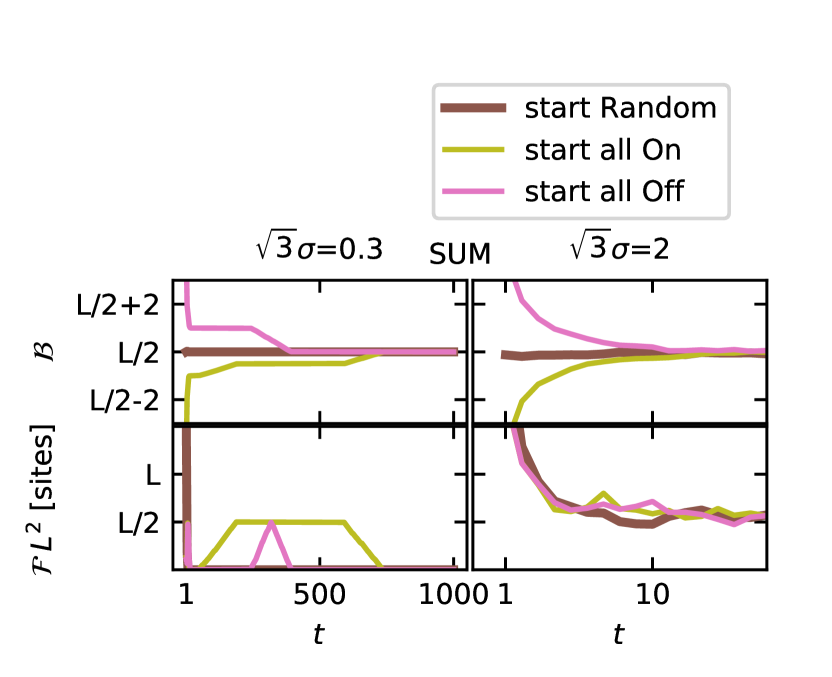
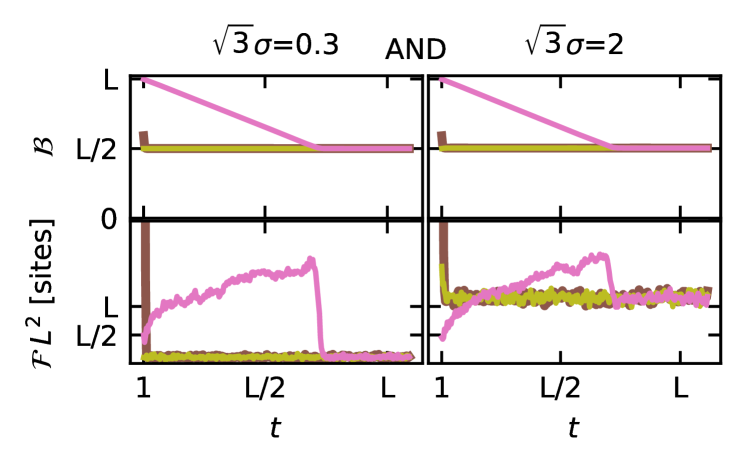
Figure 10: Exemplary time traces from simulation with same parameters as in the main text, except from the grid length, here $L=256$ sites.

Appendix E Analytics for the stationary boundary position

Condition for stationary boundary position

We have two conditions to be satisfied such that the stationary boundary position is at cell index $i=i_{c}$: The probability to destabilize a boundary at $i_{c}-1$ by an Off-in-On defect has to be smaller or equal to the probability destabilizing a boundary at $i_{c}$ by an On-in-Off defect. For a sketch, see the first grid of Fig. 2, insets (iii) and (iv), respectively. For the right-hand side of $i_{c}$ we can formulate the conditions as:

$$(i) |b=i_{c}-1 >\text{P(OnInOff $|b=i_{c}$)}$$ P(OffInOn )

$$(ii) |b=i_{c} <\text{P(OnInOff $|b=i_{c}+1$)}$$ P(OffInOn )

with, e.g., P(OffInOn $|b=i_{c}-1$) denoting the probability of an Off-in-On defect, if the sharp boundary position is at $b=i_{c}+1$.

Stationary boundary position for the SUM rule

For the SUM rule the individual probabilities are given by

P(OnInOff $$|b=i =\text{P}(s^{G}(i)+s^{L}(i)\geq a)$$)

$$=\text{P}\left(mi+\sum\limits_{(k,l)\in\mathcal{V}(i,j)}c_{k,l}+\xi\geq a\right)$$

$$=\text{P}\left(\xi\geq a+1-mi\right)\>,$$

with $\mathcal{V}(i,j)$ the Von Neumann neighborhood of the cell at $(i,j)$, i.e., its upper, lower, right, and left neighbor and $\xi=\xi^{L}+\xi^{G}$ the total noise. We at first used that with a straight boundary at $i$ a cell at $(i,j)$ ($j$ arbitrary) has one On and three Off neighbors.
Further,

P(OffInOn $$|b=i =\text{P}(s^{G}(i+1)+s^{L}(i+1)<a)$$)

$$=\text{P}\left(m(i+1)+\sum\limits_{(k,l)\in\mathcal{V}(i+1,j)}c_{k,l}+\xi<a\right)$$

$$=\text{P}\left(\xi<a-m(i+1)-1\right)\>.$$

Inserting both into conditions (i) and (ii) and that $\xi$ has the same distribution as $-\xi$ gives

$$(i) \quad\text{P}(\xi<a-mi_{c}-1)>\text{P}(\xi\leq-(a-mi_{c})-1)$$

$$\Rightarrow\quad a-mi_{c}\geq 0\>,$$

$$(ii) \quad\text{P}(\xi<a-m(i_{c}+1)-1)<$$

$$\quad\text{P}(\xi\leq-(a-m(i_{c}+1))-1)$$

$$\Rightarrow\quad a-m(i_{c}+1)<0\>.$$

As $i_{c}\in\mathbb{N}$, these two inequalities are satisfied by

$$i_{c}^{\text{SUM}}=\left\lfloor\frac{a}{m}\right\rfloor=i_{c}^{\text{Grad}}\>.$$ (15)

The stationary boundary will scale with system size in the same way as for the pure boundary formation by gradient mechanism for zero noise.
Note that in the stationary state, implying that $i=i_{c}$, the probabilities for an On-In-Off defect and an Off-In-On defect only depend on the morpophogen slope $m$ and the deviation of $\frac{a}{m}$ from its subsequent integer:

P(OffInOn $$|b=i_{c} =\text{P}\left(\xi<a-m(i_{c}+1)-1\right)$$)

$$=\text{P}\left(\xi<m\left(\frac{a}{m}-\left\lfloor\frac{a}{m}\right\rfloor+1\right)-1\right)$$

and equivalently for P(OnInOff $|b=i_{c}$).

Stationary boundary position for the AND and OR rule

Let us consider the AND rule. The individual probabilities are given by

P(OnInOff $$|b=i$$)

$$=\text{P}\left(s^{G}_{ij}(t)+\xi_{ij}^{G}(t)>a\right)\text{P}\left(\sum\limits_{(k,l)\in\mathcal{V}(i,j)}c_{k,l}+\xi_{ij}^{L}(t)\geq-1\right)$$

$$=\text{P}(s^{G}_{ij}(t)+\xi_{ij}^{G}(t)>a)\text{P}\left(\xi_{ij}^{L}(t)\geq 0\right)$$

$$=\text{P}(s^{G}_{ij}(t)+\xi_{ij}^{G}(t)>a)\frac{1}{2}\>,$$

where we at first used that with a straight boundary at $i$ a cell at $i$ has one On and three Off neighbors. Then we observed that the for nonzero noise the probability of the local noise to exceed its mean 0 is 1/2, independent of its precise distribution (as long as it is symmetric).
Further,

P(OffInOn $$|b=i$$)

$$=1-\text{P}(s^{G}_{i+1,j}+\xi_{ij}^{G}(t)>a)$$

$$\quad\quad\cdot\text{P}\left(\sum\limits_{(k,l)\in\mathcal{V}(i+1,j)}c_{k,l}+\xi_{ij}^{L}(t)\geq-1\right)$$

$$=1-\text{P}(s^{G}_{i+1,j}+\xi_{ij}^{G}(t)>a)\text{P}\left(\xi_{ij}^{L}(t)\geq-2\right)$$

$$\approx 1-\text{P}((s^{G}_{i+1,j})+\xi_{ij}^{G}(t)>a)$$

Here we used that for an Off-in-On defect given the boundary is at $i$, we need to consider a cell at $i+1$, which consequently has one Off and three On neighbors.
For the noise level regime, $\sqrt{3}\sigma\in\left[0,2.5\right]$ that we consider in this paper, $\text{P}\left(\xi^{L}\geq-2\right)\approx 1$ is a good approximation.
With that follows from condition (i)

$$\text{P}\left(s^{G}_{i_{c}^{\text{AND}},j}+\xi_{ij}^{G}(t)>a\right)<\frac{2}{3}\>,$$ (16)

which is easily satisfied for $i_{c}^{\text{Grad}}=\left\lfloor\frac{a}{m}\right\rfloor$ as $s^{G}(i_{c}^{\text{Grad}})\approx 0$.
From condition (ii) follows

$$\text{P}\left(s^{G}_{i_{c}^{\text{AND}}+1,j}+\xi_{ij}^{G}(t)>a\right)\geq\frac{2}{3}\>,$$ (17)

which consequently determines $i_{c}^{\text{AND}}$. For the Gaussian noise distribution with mean zero and standard deviation $\sigma^{G}=\sigma\sqrt{1-\frac{2}{2+mL}}$, it follows

$$i_{c}^{\text{AND}} =\left\lfloor\frac{a}{m}\right\rfloor-\frac{\sqrt{3}\sigma}{m}\sqrt{1-\frac{2}{2+mL}}\left(\sqrt{\frac{2}{3}}\text{erfc}^{-1}\left(\frac{4}{3}\right)\right)$$

$$\approx\left\lfloor\frac{a}{m}\right\rfloor+0.25\frac{\sqrt{3}\sigma}{m}\sqrt{1-\frac{2}{2+mL}}\>.$$ (18)

We see that $i_{c}^{\text{AND}}\approx i_{c}^{\text{Grad}}+\frac{\sqrt{3}\sigma}{4m}$ for $mL\gg 2$, which agrees nicely with simulation results shown in Fig. 3.
For the OR rule, it follows

$$i_{c}^{\text{OR}}\approx\left\lfloor\frac{a}{m}\right\rfloor-0.25\frac{\sqrt{3}\sigma}{m}\sqrt{1-\frac{2}{2+mL}}\>,$$ (19)

respectively by the AND-OR equivalence established in Eq. (6).

Appendix F Convergence during Scaling

The reason the boundary position and fuzziness for small lengths deviate from the values for large grids is of technical nature, as our parameter choice yields a boundary at $\left\lfloor\frac{a}{m}\right\rfloor=\frac{a}{m}=\frac{1}{4}L$. For the pure gradient rule, for instance, this choice implies

$$c_{i_{c},j}=\Theta(mi_{c}+\xi_{ij}^{G}(t)\geq a)-\frac{1}{2}=\Theta(\xi_{ij}^{G}(t)\geq 0)-\frac{1}{2}\>,$$

and thus on average the cell at $i_{c}$ is switched On every second time step due to noise. In contrast, for $c_{(i_{c}+1,j)}$ these parameters more stably yield On as

$$c_{i_{c}+1,j}=\Theta(mi_{c+1}+\xi^{G}_{i_{c}+1,j}\geq a)-\frac{1}{2}=\Theta(\xi^{G}\geq-m)-\frac{1}{2}\>.$$

Thus defect cells at the left of the boundary are more common than at its right.

References

- Dahmann et al. [2011] C. Dahmann, A. C. Oates, and M. Brand, Boundary formation and maintenance in tissue development, Nature Reviews Genetics 12, 43 (2011).
- Barkai and Shilo [2020] N. Barkai and B.-Z. Shilo, Reconstituting tissue patterning., Science (New York, N.Y.) 370, 292 (2020).
- Wolpert [1969] L. Wolpert, Positional information and the spatial pattern of cellular differentiation, Journal of Theoretical Biology 25, 1 (1969).
- Gregor et al. [2007] T. Gregor, D. W. Tank, E. F. Wieschaus, and W. Bialek, Probing the Limits to Positional Information, Cell 130, 153 (2007).
- Zagorski et al. [2017] M. Zagorski, Y. Tabata, N. Brandenberg, M. P. Lutolf, T. Bollenbach, J. Briscoe, , and A. Kicheva, Decoding of position in the developing neural tube from antiparallel morphogen gradients, Science 356, 1379 10.1126/science.aam5887 (2017).
- Petkova et al. [2019] M. D. Petkova, G. Tkačik, W. Bialek, E. F. Wieschaus, T. Gregor, Optimal Decoding of Cellular Identities in a Genetic Network, Cell 176, 10.1016/j.cell.2019.01.007 (2019).
- Aliee et al. [2012] M. Aliee, J. C. Röper, K. P. Landsberg, C. Pentzold, T. J. Widmann, F. Jülicher, C. Dahmann, Physical mechanisms shaping the Drosophila dorsoventral compartment boundary, Current Biology 22, 10.1016/j.cub.2012.03.070 (2012).
- Lander [2013] A. D. Lander, How cells know where they are, Science 339, 923 (2013).
- Bollenbach et al. [2008] T. Bollenbach, P. Pantazis, A. Kicheva, C. Bökel, M. González-Gaitán, and F. Jülicher, Precision of the Dpp gradient, Development 135, 1137 (2008).
- Jaeger et al. [2008] J. Jaeger, D. Irons, and N. Monk, Regulative feedback in pattern formation: Towards a general relativistic theory of positional information, Development 135, 3175 (2008).
- Exelby et al. [2021] K. Exelby, E. Herrera-Delgado, L. G. Perez, R. Perez-Carrasco, A. Sagner, V. Metzis, P. Sollich, and J. Briscoe, Precision of tissue patterning is controlled by dynamical properties of gene regulatory networks, Development (Cambridge) 148, 10.1242/dev.197566 (2021).
- Perrimon et al. [2012] N. Perrimon, C. Pitsouli, and B. Z. Shilo, Signaling mechanisms controlling cell fate and embryonic patterning, Cold Spring Harbor Perspectives in Biology 4, a005975 (2012).
- Levin [2021] M. Levin, Bioelectric signaling: Reprogrammable circuits underlying embryogenesis, regeneration, and cancer, Cell 184, 1971 (2021).
- Toda et al. [2020] S. Toda, W. L. Mckeithan, T. J. Hakkinen, and P. Lopez, Engineering synthetic morphogen systems that can program multicellular patterning, Science 370, 327 (2020).
- Stapornwongkul et al. [2020] K. S. Stapornwongkul, M. De Gennes, L. Cocconi, G. Salbreux, and J.-P. Vincent, Patterning and growth control in vivo by an engineered GFP gradient, Science 6514, 321 (2020).
- Toda et al. [2019] S. Toda, N. W. Frankel, and W. A. Lim, Engineering cell – cell communication networks: programming multicellular behaviors, Current Opinion in Chemical Biology 52, 31 (2019).
- Barbier et al. [2020] I. Barbier, R. Perez‐Carrasco, and Y. Schaerli, Controlling spatiotemporal pattern formation in a concentration gradient with a synthetic toggle switch, Molecular Systems Biology 16, 1 (2020).
- van Gestel et al. [2021] J. van Gestel, T. Bareia, B. Tenennbaum, A. Dal Co, P. Guler, N. Aframian, S. Puyesky, I. Grinberg, G. G. D’Souza, Z. Erez, M. Ackermann, and A. Eldar, Short-range quorum sensing controls horizontal gene transfer at micron scale in bacterial communities, Nature Communications 12, 2324 (2021).
- Hillenbrand et al. [2016] P. Hillenbrand, U. Gerland, and G. Tkačik, Beyond the French Flag Model: Exploiting Spatial and Gene Regulatory Interactions for Positional Information, PloS one 11, e0163628 (2016).
- Buchler et al. [2003] N. E. Buchler, U. Gerland, and T. Hwa, On schemes of combinatorial transcription logic, Proceedings of the National Academy of Sciences of the United States of America 100, 5136 (2003).
- Mayo et al. [2006] A. E. Mayo, Y. Setty, S. Shavit, A. Zaslaver, and U. Alon, Plasticity of the cis-regulatory input function of a gene, PLoS Biology 4, 555 (2006).
- Sup [2022] Supplementary material for I. Details on boundary position and fuzziness definition; II. Comparison to an asynchronous update scheme; III. Kinetics of the correction mechanism in detail; IV. Comparison of the Ising model. (2022).
- Raser and O’Shea [2005] J. M. Raser and E. O’Shea, Noise in Gene Expression, Science 309, 2010 (2005).
- Restrepo et al. [2014] S. Restrepo, J. J. Zartman, and K. Basler, Coordination of patterning and growth by the morphogen DPP, Current Biology 24, R245 (2014).
- Colman-Lerner et al. [2005] A. Colman-Lerner, A. Gordon, E. Serra, T. Chin, O. Resnekov, D. Endy, C. G. Pesce, and R. Brent, Regulated cell-to-cell variation in a cell-fate decision system, Nature 437, 699 (2005).
- Bolouri and Davidson [2002] H. Bolouri and E. H. Davidson, Modeling transcriptional regulatory networks, BioEssays 24, 1118 (2002).
- Kalir and Alon [2004] S. Kalir and U. Alon, Using a quantitative blueprint to reprogram the dynamics of the flagella gene network, Cell 117, 713 (2004).
- Inomata [2017] H. Inomata, Scaling of pattern formations and morphogen gradients, Development Growth and Differentiation 59, 41 (2017).
- Field and Rieke [2002] G. D. Field and F. Rieke, Nonlinear Signal Transfer from Mouse Rods to Bipolar Cells and Implications for Visual Sensitivity photons, Neuron 34, 773 (2002).
- Bialek [2012] W. Bialek, Biophysics: Searching for Principles (Princeton University Press, New Jersey, 2012) p. 640.
- Bashor et al. [2019] C. J. Bashor, N. Patel, S. Choubey, A. Beyzavi, J. Kondev, J. J. Collins, and A. S. Khalil, Complex signal processing in synthetic gene circuits using cooperative regulatory assemblies, Science (New York, N.Y.) 597, 593 (2019).
- Chen and Elowitz [2021] Z. Chen and M. B. Elowitz, Programmable protein circuit design, Cell , 1 (2021).