Motion control with optimal nonlinear damping: from theory to experiment

Abstract

Optimal nonlinear damping control was recently introduced for the second-order SISO systems, showing some advantages over a classical PD feedback controller. This paper summarizes the main theoretical developments and properties of the optimal nonlinear damping controller and demonstrates, for the first time, its practical experimental evaluation. An extended analysis and application to more realistic (than solely the double-integrator) motion systems are also given in the theoretical part of the paper. As comparative linear feedback controller, a PD one is taken, with the single tunable gain and direct compensation of the plant time constant. The second, namely experimental, part of the paper includes the voice-coil drive system with relatively high level of the process and measurement noise, for which the standard linear model is first identified in frequency domain. The linear approximation by two-parameters model forms the basis for designing the PD reference controller, which fixed feedback gain is the same as for the optimal nonlinear damping control. A robust sliding-mode based differentiator is used in both controllers for a reliable velocity estimation required for the feedback. The reference PD and the proposed optimal nonlinear damping controller, both with the same single design parameter, are compared experimentally with respect to trajectory tracking and disturbance rejection.

1 INTRODUCTION

For the second-order systems it is understood that a linear feedback control, see e.g. [4] for basics, has certain limitations in shaping the transient dynamics and therefore the asymptotic convergence of the controlled output of interest. In a standard state-space form

$$[\dot{x}_{1},\dot{x}_{2}]^{T}=A\cdot[x_{1},x_{2}]^{T}=\left[\begin{array}[]{cc}0&1\\ -k&-d\\ \end{array}\right]\cdot[x_{1},x_{2}]^{T},$$ (1)

the system matrix $A$ can be arbitrary shaped as Hurwitz via the state-feedback coefficients $k,d>0$. Needless to dive into detail that both coefficients can accommodate the own system dynamics as well as the control gains. It is also worth recalling that a standard linear proportional-derivative (PD) control, which is sufficient for the unperturbed second-order systems, can be easily integrated into the state-space form (1). Assuming the output feedback gain $k$ is fixed by some dedicated control specification or policy, like for example control saturations or measurement noise, one can assign the linear damping term by solving the associated characteristic polynomial

$$s^{2}+ds+k=(s+\lambda)^{2}$$ (2)

with respect to $d$. Here the real double pole at $-\lambda$ is optimal in terms of the damping (usually referred to as critical damping). Namely, it shapes the control system in such a way that it has neither a dominant (and thus slower) pole if $d>2\lambda$, nor it oscillates transiently if $d<2\lambda$. It follows that the linearly damped second-order dynamics of a feedback control system of the type (1) cannot perform any better convergence, in the sense of an optimal damping rate, than that provided by the real double pole. Few counterexamples can be found, like for instance one of the optimal damping ratio for the linear second-order systems which, however, requires the system damping to be switched as a function of the system state [16]. Also a comparative evaluation of different controllers [11], benchmarking for simplest second-order system of a double integrator, can be mentioned here as an associated reference.

The motion control systems often deal with the second-order dynamics, in which the relative displacement $x_{1}$ and its rate $x_{2}$ (i.e. velocity) of the moving tools and loads (in a more general sense) are the state variables in focus. Practical examples can range from the accurate micro- and nano-positioning [6, 5] to the standard robotic manipulators [1, 3], just exemplary referring to more former and more recent developments. Already in the earlier works on the control in robotics, see e.g. [18], it was recognized that a simple PD feedback control is sufficient for regulation, once the main system nonlinearities are compensated by either inverse dynamics control or torque feed-forwarding. However, a certain temptation of incorporating also nonlinear damping into the feedback of the second-order systems, with the aim of improving the stabilization and convergence properties, was occasionally made. This was denoted, again in context of robotics, by the so-called nonlinear proportional-derivative controllers, see e.g. [19, 7]. Recently, an optimal nonlinear damping (OND) control, as combination with the standard proportional output feedback, was proposed in [14] for the unperturbed second-order systems. This forms the basis of the present work.

In this paper, we provide a practice oriented transition from the theory to experiments for the OND control applied to the motion control tasks. For the sake of a fair comparison, we also design a robust PD feedback controller, which serves as a reference one, and we stress that both controllers have only one and the same tunable parameter – the overall control gain. Since steering the residual control errors towards zero is not our prime focus here, it is explicitly emphasized that no additional integral control actions are considered, so that a fair comparison to a standard PID feedback control is not made. At this point, it is worth noting that extension of the optimal nonlinear damping control by an (eventually) nonlinear integral action might be an interesting future research that requires further fundamental and extensive investigations. Moreover one should state that the developed OND control is suitable for the SISO systems, while a potential MIMO extension is also subject to the future works. The rest of the paper is divided into two main parts, theoretical and experimental, accommodated in sections 2 and 3, correspondingly. The main conclusions are drawn in section 4 at the end of the paper. The theoretical developments from section 2 were partially presented in [13]. To complete the introduction, the overall contribution of the paper can be summarized as follows.

• The optimal nonlinear damping control of the second-order systems, proposed in [14, 13], is provided in a consolidated manner for practical motion control applications. It includes a regularization factor, which extends the non-singular trajectory solutions to the whole $\mathbb{R}^{2}$ state-space of the motion variables.

• Further theoretical developments and adjustments, in relation to the damped and perturbed motion system dynamics, are included. The motion system dynamics, identifiable in frequency domain, is addressed in regard to the control parametrization and tuning.

• Experimental evaluation of the nonlinear damping control is shown, for the first time, on a real drive system with inherent measurement and process noise. Robust sliding-mode differentiator is used for the not measurable relative velocity required for the feedback control. In addition, the proposed optimal nonlinear damping control is compared experimentally with a robustly designed linear PD feedback control.

2 THEORETICAL PART

In this section, which is the theoretical part, we will summarize the OND control which was first introduced in [14] and later shown in [13] to have the convergent dynamics with an augmented regularization factor. The convergent dynamics, see [10], will be briefly recalled for convenience of the reader. It will also be shown how to apply the OND control to the motion systems which have additional first-order time delay dynamics and are, eventually, perturbed. For those classical motion plants, we will also discuss the design of a reference PD control, which can be tuned by only one free parameter, similar as the OND control. Such design complexity renders both controllers well comparable in a benchmarking.

2.1 Optimal nonlinear damping control

The second-order closed-loop control system with an optimal nonlinear damping is written as (cf. [14])

$$\dot{x}_{1} = x_{2},$$ (3)

$$\dot{x}_{2} = -kx_{1}-x_{2}^{2}|x_{1}|^{-1}\mathrm{sign}(x_{2}),$$ (4)

where $k>0$ is an arbitrary control design parameter. Note that feedback control with the nonlinear damping term as in (4) was introduced first for unperturbed double-integrator systems only. The system (3), (4), where $x_{1}$ is the output of interest, is globally asymptotically stable and converges to the unique equilibrium in the origin. This occurs: (i) along an attractor

$$x_{2}+\sqrt{k}x_{1}=0$$ (5)

in vicinity to the origin, and (ii) without crossing the $x_{2}$-axis, see Figure 1.

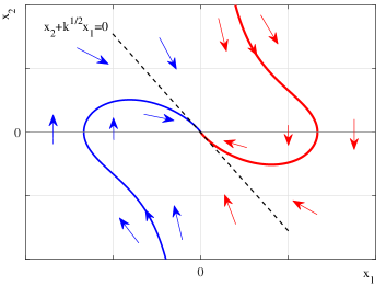
Figure 1: Phase portrait of the closed-loop system (3), (4).

Note that the (ii)-nd property prevents singularity, which is otherwise due to $x_{1}=0$ when $x_{2}(t)\neq 0$. It can be shown that the closed-loop dynamics (3), (4) is always repulsing the state trajectories away from the $x_{2}=0$ axis, except from $(x_{1},x_{2})=\mathbf{0}$ equilibrium. The latter is global and asymptotically attractive. Therefore, the admissible set of the initial conditions for (3), (4) is $X_{0}(t=0)=\bigl{\{}(x_{1},x_{2})\in\mathbb{R}^{2}\>|\>x_{1}\in\mathbb{R}^{*}\bigr{\}}$, where $\mathbb{R}^{*}$ is the set of real numbers without null. The OND control does not requires any gain (i.e tuning) parameter for the nonlinear damping term, and the single output feedback gain $k$ is scaling the transient response of both dynamic state trajectories, as exemplary shown in Figure 2. It is also worth recalling that the closed-loop control system (3), (4) allows for a bounded control action $|\dot{x}_{2}|<S$, with $S=\mathrm{const}>0$. Such saturated control action, especially relevant for practical applications, affects neither stability nor convergence properties of the state trajectories, as shown in [14].

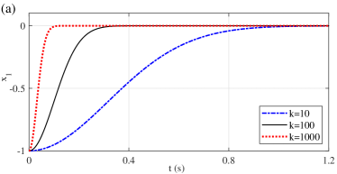
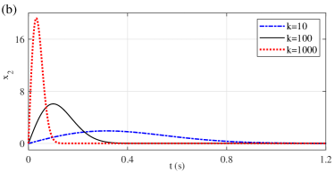
Figure 2: State trajectories $x_{1}(t)$ in (a) and $x_{2}(t)$ in (b) for the varying values of the control gain $k=[10,\,100,\,1000]$.

In order to allow for the state trajectories in the whole $(x_{1},x_{2})\in\mathbb{R}^{2}$ state-space and, therefore, to avoid singularity when crossing the $x_{2}$-axis outside the origin, a regularization term $0<\mu\ll k$ was later introduced in [13]. Moreover, the OND control was extended for tracking the differentiable (at least once) reference trajectories $r(t)\in\mathcal{C}^{1}$. For such reference signals, the OND control performance is guaranteed for $\ddot{r}(t)=0$, which can be seen as steady-state for the motion control. For any $\dot{r}(t)\neq\mathrm{const}$ finite-time (i.e. $t<T$) transient phase trajectory, the OND control becomes temporary perturbed. Then, i.e. for $t>T$, the OND control converges according to the $(e_{1},e_{2})(t)$ error dynamics, where the output error state is $e_{1}=x_{1}-r$ and its time derivative is $\dot{e}_{1}\equiv e_{2}=x_{2}-\dot{r}$, respectively. The state error dynamics of the regularized OND control, which is applied to the double-integrator system, reads

$$\dot{e}_{1} = e_{2},$$ (6)

$$\dot{e}_{2} = -ke_{1}-\frac{|e_{2}|\,e_{2}}{|e_{1}|+\mu}.$$ (7)

Note that the regularization term $\mu$ does not act as an additional control gain, to be designed, but prevents singularity in solutions of the closed-loop system (3), (4). When assuming a quadratic Lyapunov function candidate

$$V=\frac{1}{2}ke_{1}^{2}+\frac{1}{2}e_{2}^{2},$$ (8)

which represents the total energy level (i.e. potential energy of the feedback control plus kinetic energy of the relative motion), its time derivative results in

$$\frac{d}{dt}V=-\frac{|e_{2}|\,e_{2}^{2}}{|e_{1}|+\mu}.$$ (9)

It can be recognized that while $V$ is positive definite and radially unbounded, its time derivative (9) is negative definite $\forall\>e_{2}\neq 0$ only. Applying the standard invariance principle by LaSalle, one can easily show that for $e_{2}=0$ outside the origin, the vector field $\dot{e}_{2}=-ke_{1}$ will always push a trajectory away from $e_{2}$-axis, where $\dot{V}$ becomes negative definite. This proves the global asymptotic stability of the unique equilibrium $(e_{1},e_{2})=\mathbf{0}$.

A clarifying aspect of the nonlinear damping properties of (6), (7) highlights when analyzing the rate at which the control system reduces its energy, based on (9). From both projection of $|\dot{V}|$, shown in Figure 3 (a) and (b), one can recognize that the energy rate is hyperbolic in the error size, i.e. $\sim|e_{1}|^{-1}$, and cubic in the error rate, i.e. $\sim|e_{2}|^{3}$.

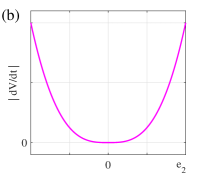
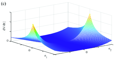
Figure 3: Energy reduction rate $|\dot{V}|$ of the system (6), (7): depending on $e_{1}$ in (a), depending on $e_{2}$ in (b), and as overall error-states function according to (9) in (c).

From Figure 3 (a), one can also recognized that the regularization term $\mu$ prevents an infinite energy rate and, thus, ensures a finite control action as $|e_{1}|\rightarrow 0$. At the same time, a hyperbolic energy rate allows accelerating the convergence as $|e_{1}|\rightarrow 0$. On the other hand, it is the cubic dependency from the error rate which enables the OND control reacts faster to the error dynamics, cf. Figure 3 (b). This property is especially relevant for non-steady trajectory phases, i.e. $\ddot{r}(t)\neq 0$, or when perturbations provoke a fast growth of the $|e_{2}|$-value. The overall landscape of the energy dissipation rate, see Figure 3 (c), discloses that this is lower in magnitude larger the control error norm $\|e_{1},e_{2}\|$ is. For decreasing $\|e_{1},e_{2}\|(t)$, and that when $|e_{1}|\rightarrow 0$, the $|\dot{V}|$ is largely growing, thus, allowing for faster decelerations and convergence of the controlled motion in vicinity to the reference trajectory.

For better interpreting transient performance of the OND control, let us compare it with the standard linear PD feedback control, for which the error dynamics (7) transforms to $\dot{e}_{2}=-ke_{1}-k\,\tau e_{2}$, where $\tau$ is the time constant parameter. Obviously, the $k$ and $\tau$ parameters can be assigned so that the linear closed-loop dynamics is critically damped, i.e. has a negative double real pole at the desired location. For the following numerical example, let us assume $k=100$ and $\tau=0.2$, resulting in the double real pole at $-10$. Note that we assume the same $k=100$ for the OND control, given by (6), (7), while $\mu=0.0001\ll k$ is assigned. The piecewise linear trajectory $r(t)$, that is typical for motion control tasks, is exemplary shown in Figure 4 (a), together with the OND controlled output trajectory. The difference in transient response between the OND control and critically damped PD control, both having the same feedback gain factor, is best visible in the $x_{2}(t)$ trajectories shown in Figure 4 (b).

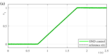
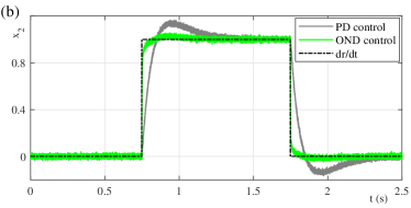
Figure 4: Reference trajectory versus OND controlled output position in (a), and comparison of the corresponding velocity for OND and PD control in (b). Both controllers have the same feedback gain factor $k=100$, while $\mu=0.0001$ is assumed for OND control.

The convergence properties of both controllers become even more evident when assuming $r=0$ and $x_{1}(0)\neq 0$ and comparing the $x_{1}(t)$ trajectories plotted on the logarithmic scale, see Figure 5. While the linear PD control shows the (expected) linear-shaped convergence on the logarithmic scale, the OND control discloses a hyper-exponential (e.g. quadratic on the logarithmic scale) convergence of $|x_{1}|(t)$. It is easy to recognize that the difference and, therefore, advantage of the OND control becomes more considerable, higher the control accuracy and, correspondingly, lower residual error $e_{1}(t)\,|\,_{t\rightarrow\infty}$ are required.

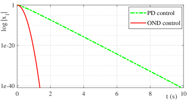
Figure 5: Convergence of the controlled output value of the PD and OND controllers (logarithmic absolute value).

2.2 Convergent dynamics

Below, we briefly recall the main statements and properties of a dynamic system to be convergent, according to [2], while for more details we refer to [10], and for the convergent system (6), (7) to [13].

Definition 1. The system $\dot{x}=f(x,t)$ is said to be convergent if for all initial conditions $t_{0}\in\mathbb{R}$, $\bar{x}_{0}\in\mathbb{R}^{n}$ there exists a solution $\bar{x}(t)=x(t,t_{0},\bar{x}_{0})$ which satisfies:

1. $\bar{x}(t)$ is well-defined and bounded for all $t\in(-\infty,\infty)$;

2. $\bar{x}(t)$ is globally asymptotically stable.

Such solution $\bar{x}(t)$ is called a limit solution, to which all other solutions of the dynamic system converge as $t\rightarrow\infty$.

Theorem 1. Consider the system $\dot{x}=f(x,t)$. Suppose, for some positive definite matrix $P=P^{T}>0$ the matrix

$$J(x,t):=\frac{1}{2}\Bigl{(}P\,\frac{\partial f}{\partial x}(x,t)+\Bigl{[}\frac{\partial f}{\partial x}(x,t)\Bigr{]}^{T}P\Bigr{)}$$ (10)

is negative definite uniformly in $(x,t)\in\mathbb{R}^{n}\times\mathbb{R}$ and $|f(0,t)|\leq\mathrm{const}<+\infty$ for all $t\in\mathbb{R}$. Then the system is convergent. The detailed proof can be found in [10].

Evaluating the Jacobian of $f(x,t)$ of the system (6), (7) with $x=[e_{1},\,e_{2}]^{T}$ and suggesting

$$P=\frac{1}{2}\,\left[\begin{array}[]{cc}k&0\\ 0&1\\ \end{array}\right],$$ (11)

which is the positive definite matrix, one can show that the matrix $J(x,t)$, which is the solution of (10), is negative definite and, hence, the Theorem 1 holds. For proving it, we evaluate the matrix definiteness as

$$x^{T}J(x,t)\,x=-\frac{3}{4}\,\frac{|e_{2}|\,e_{2}^{2}\,\bigl{(}|e_{1}|+2\mu\bigr{)}}{\bigl{(}e_{1}+\mu\,\mathrm{sign}(e_{1})\bigr{)}^{2}}\,\leq 0\quad\forall\;x\neq 0.$$ (12)

Note that the obtained inequality (12) proves only the negative semi-definiteness of $J(x,t)$, since $x^{T}J(x,t)\,x=0$ for $e_{2}=0\,\wedge\,e_{1}\neq 0$. It is however possible to show that $[e_{1},\,e_{2}]=0$ is the unique limit solution by evaluating the $\dot{e}_{2}$ dynamics at $e_{2}=0$. Substituting $e_{2}=0$ into (7) results in $\dot{e}_{2}=-ke_{1}$. It implies that $[e_{1}\neq 0,\,e_{2}=0](t)$ cannot be a limit (correspondingly steady-state) solution, since any trajectory will be repulsed away from $e_{2}=0$ as long as $e_{1}\neq 0$. Therefore, the closed-loop control system (6), (7) is uniformly convergent. Consequently, the origin in the control error coordinates $[e_{1},e_{2}](t)=0\equiv\bar{x}$ is the unique limit solution for $\forall\>t_{0}<\tau<t$, independently of the initial conditions $[e_{1},e_{2}](t_{0})$.

2.3 Control extension for common motion systems

The practical motion systems, associated with the controlled drives, contain usually the additional damping dynamics and input gain parameters, so that a system to be controlled is no longer just the double integrator, cf. (3), (4). Without restoring force actions and, therefore, having one free integrator (in terms of $\dot{x}_{1}=x_{2}$), the motion dynamics which is driven by the control input $u$ can be most simply modeled by

$$\tau\dot{x}_{2}(t)+x_{2}(t)=Ku(t).$$ (13)

Here, the time constant $\tau=m\,\sigma^{-1}$ results from the overall moving mass $m$ and linear (viscous) damping coefficient $\sigma$, while $K$ is the overall input gain which converts the available control channel into the generalized force quantity. The latter is, correspondingly, actuating the drive system according to the Newton’s laws of motion. Obviously, such linear system (13) can be directly transformed into Laplace domain and then identified (i.e. also in frequency domain). The latter will result in determining only two free parameters, $\tau$ and $K$, when using the input $u(t)$ and available output measurement, either $x_{1}(t)$ or $x_{2}(t)$, cf. with the experimental part provided in section 3.

For motion systems, which are not the free double-integrator but have dynamics of the form (13), the parametric scaling of the OND control is required. This is in order the closed-loop control system keeps the same stability and convergence properties as for (6), (7). First, consider the system plant (13) without its linear damping term. Substituting the OND control instead of $u$ results in

$$\dot{x}_{2}(t)=\frac{K}{\tau}\bigl{(}\mathcal{P}+\mathcal{D}\bigr{)},$$ (14)

where the proportional and damping control parts are abbreviated (for the sake of clarity) by $\mathcal{P}$ and $\mathcal{D}$, correspondingly, cf. (3), (4). Recall that the proportional control part $\mathcal{P}=-k(x_{1}-r)$ allows for any positive gain values $k>0$, without affecting the basic properties of OND control, cf. [14, 13]. Therefore, no scaling of $\mathcal{P}$ is required. At the same time, one can recognize that an inverse gaining factor $\tau/K$ must be incorporated into $\mathcal{D}$ for keeping the left- and right-hand side of (14) as balanced as in the original OND control, cf. (4). Now, taking back into account the linear system damping, which is scaled by $\tau^{-1}$ cf. with (13), one obtains the closed-loop dynamics

$$\dot{x}_{2}(t)+\frac{1}{\tau}x_{2}(t)=\frac{K}{\tau}\bigl{(}\mathcal{P}+\mathcal{D}\bigr{)},$$ (15)

with the scaled damping control part

$$\mathcal{D}=-\frac{\tau}{K}\,\frac{|e_{2}|\,e_{2}}{|e_{1}|+\mu}.$$ (16)

Through the applied scaling of the OND control in (16), the inertial (on the left-hand side) and control (on the right-hand side) terms in (15) will represent the nonlinear differential equation with the same convergence properties as (7). However, the linear damping term (on the left-hand side of (15)) appears now as a disturbing factor. This can be compensated by direct inclusion into the control law, i.e. on the right-hand side of (15). The resulted control law of the scaled OND with an additional compensation of the system damping term is

$$u(t)=\mathcal{P}+\mathcal{D}+\frac{1}{K}x_{2}(t).$$ (17)

Now, taking into account that the nominal motion dynamics (13) can be perturbed by some upper bounded disturbance $|\xi|\leq\mathrm{const}$, the closed-loop behavior of the plant (13) with the control (17) results in

$$\tau\ddot{x}_{1}+\tau\frac{|\dot{x}_{1}|\dot{x}_{1}}{|x_{1}|+\mu}+kx_{1}=\xi,$$ (18)

when assuming $r=0$, for the sake of simplicity, and some non-zero initial conditions $(x_{1},x_{2})(t)\neq 0$ for the sake of analysis. It can be seen that the second-order nonlinear differential equation (18) remains asymptotically stable, cf. sections 2.1 and 2.2, while no longer converging to zero equilibrium but to $x_{1}(t)\rightarrow\xi k^{-1}$ at steady-state. This indicates how large the static position control error is, just as in case of standard PD feedback controllers when they are affected by the matched perturbations. If the matched perturbation $\xi(t)$ appears dynamically, the convergence of the OND control will always be faster than that of a classical PD controller, cf. Figure 5.

2.4 Design of reference PD controller

As a reference PD feedback controller, we assume the one which has the following form

$$u(t)=\gamma\bigl{(}r(t)-x_{1}(t)\bigr{)}-\gamma\tau x_{2}(t),$$ (19)

with the design gain factor $\gamma$ and given parameter $\tau$. The latter compensates directly for the time constant of the system plant, cf. (13), this way making the PD control (19) to a simply tunable one-parameter feedback regulator. Note that solely the control error $e(t)\equiv r(t)-x_{1}(t)$ is subject to the proportional control amplification, while the differential control part with the total gaining by $\gamma\tau$ is using the output velocity and not $\dot{e}(t)$. This allows applying also the discontinuous reference signals, like e.g. a step, for which $\dot{r}$ does not exist. For analyzing optimality of parametrization of the PD control (19), one can easily extend the right-hand-side of (19) by $\gamma\tau\dot{e}(t)$ and, after substituting $u(t)$ into (13), obtain the open-loop transfer function in Laplace domain as

$$x_{1}s(\tau s+1)=K\gamma\,e(\tau s+1).$$ (20)

Obviously, the pole-zero cancelation in (20) converts the open-loop transfer function into the simple integrator which is amplified by the factor $K\gamma$. Transforming it back into time domain and writing out the control error gives

$$\dot{x}_{1}(t)+K\gamma\,x_{1}(t)=K\gamma\,r(t).$$ (21)

This yields a principal first-order closed-loop dynamics which has zero steady-state error and a time constant which is arbitrary assignable through the control gain $\gamma$. In practical applications, a motion system (13) will have also some neglected or parasitic (additional) dynamics at higher-frequencies and, thus, a deteriorated phase response (in terms of a phase margin) as implication. Therefore, the control gain $\gamma$ needs to be assigned with respect to the resulted cross-over frequency and the associated stability margins, cf. the practical part in section 3.3.

3 EXPERIMENTAL PART

This section is dedicated to an experimental case study, showing practical applicability and resulted performance of the OND control. The block diagram of the entire closed-loop control system, designed according to the section 2 and evaluated experimentally as follows, is depicted in Figure 6. The second-order plant of a motion system includes the free integrator and dynamics (13),

Figure 6: Block diagram of the closed-loop control system.

Note that both controllers in use, i.e. either PD or OND one, are served by the same input signals, – the reference value $r(t)$, the measured system output $x_{1}(t)$, and its derivative $y_{1}(t)$, obtained by means of the SMD, cf. with section 3.2.

3.1 Second-order motion system with voice-coil drive

The second-order motion system under investigation is the voice-coil drive, shown in the laboratory setting in Figure 7. The electro-magnetically actuated voice-coil motor has the total linear stroke about 20 mm, which is indirectly measured by the contactless inductive displacement sensor with a nominal repeatability of $\pm 12$ $\mu m$.

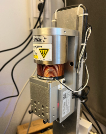
Figure 7: Experimental setup of the voice-coil drive with 1DOF.

Due to a specific attachment of the moving rigid bar, which is entering detection area of the contactless sensor, the effective measurement range and, therefore, displacement operation range $x_{1}$ of the drive is limited to about 13 mm only. The system discloses a relatively large sensor and process noise. The former is due to contactless sensing, while the latter is due to additional parasitic dynamic by-effects which are not captured by the second-order motion dynamics. The nominal electrical time constant, which is however neglected when modeling the motion dynamics is 1.2 msec. The real-time control board operates the system with the set sampling rate of 10 kHz, while the available control signal is the power-amplified voltage $U$ in the range $[0,\,10]$ V. The overall voice-coil motor resistance is $R=5.23$ Om, while the nominal motor force constant is $\Psi=17.16$ N/A. The overall moving mass of the drive, determined by the scale measurement of the parts and technical data-sheet of the drive, is $m=0.538$ kg.

The hardware specific properties of the voice-coil motor drive require the following measures to be taken with the input and output signal channels, so as to apply the feedback control provided in section 2. When neglecting the non-modeled dynamics of electro-magnetic circuit, the input force constant is $K_{u}=\Psi R^{-1}$. Note that $K_{u}$ factor has the N/V units, since mapping the input voltage $U$ to the induced input motor force $u$, and is linked to the overall input gain by $K=K_{u}\sigma^{-1}$, cf. (13). The voice-coil motor drive in its vertical arrangement, cf. Figure 7, is subject to the constant gravity force $mg$, where $g=9.8$ m/s² is the gravitational acceleration constant. Furthermore, the stator-mover configuration of the voice-coil motor gives rise the to the periodic force ripples, which act as a ’magnetic stiction’ force when the motor starts to move. In order to overcome it, a square pulse jitter signal $U_{j}$ of a low amplitude 0.2 V and high frequency 450 rad/sec is used. The suitable amplitude and frequency are found (experimentally) so that to not induce an effective motion above the measurement noise of the displacement sensor, on the one hand. On the other hand, the oscillating jitter signal should be sufficient to overcome the periodic position-dependent force ripples. The determined jitter frequency is also clearly above the bandwidth and, thus, cutoff frequency of the designed feedback controllers. By incorporating the above mentioned jitter and gravity compensation signals, the overall control voltage becomes

$$U(t)=U_{j}(t)+\frac{mg}{K_{u}}+u(t),$$ (22)

where the feedback control signal $u(t)$ takes explicitly into account the input gain $K_{u}$, cf. section 2.3.

3.2 Robust sliding-mode based differentiator

Since both the OND and the reference PD controllers require the unavailable $x_{2}(t)$-signal in feedback, its trustfully estimated value must be obtained from the measured $x_{1}(t)$. Applying a real-time discrete-time differentiation of the $x_{1}(t)$-signal does not provide an operational and robust solution for feedback of the velocity feedback. This is due to the measured position (cf. section 3.1 above) contains the broadband components of process and measurement noise and, therefore, does not necessarily hold a sufficient SNR (signal-to-noise ratio). The differentiated signals from the position measurement require mostly a low-pass filtering which inserts an additional phase lag into the control loop. This can largely restrict the achievable bandwidth of the control system and, generally, reduce the closed-loop performance at higher angular frequencies.

Robust differentiators [8], which are based on the sliding-mode principles see e.g. [17], provide an alternative for obtaining the fast estimation of relative velocity in real-time. Here the remarkable features are an insensitivity to the bounded noise (provided the Lipschitz constant of n-th time-derivative is available) and a finite-time convergence. The latter makes a robust sliding-mode based differentiator theoretically free of a phase lag which is, otherwise, unavoidable for the low-pass filtering. Assuming the estimation error of the robust sliding-mode based differentiator (further as SMD) is $\varepsilon(t)=y_{0}(t)-x_{1}(t)$, the second-order SMD, cf. [9], is given by

$$\dot{y}_{0} = -\kappa_{0}|\varepsilon|^{2/3}\mathrm{sign}(\varepsilon)+y_{1},$$ (23)

$$\dot{y}_{1} = -\kappa_{1}|\varepsilon|^{1/3}\mathrm{sign}(\varepsilon)+y_{2},$$ (24)

$$\dot{y}_{2} = -\kappa_{2}\mathrm{sign}(\varepsilon).$$ (25)

Note that the second-order (and not first-order) SMD is purposefully assumed here, in order to obtain a smoother estimate $y_{1}(t)$ of the relative velocity. Recall that the robust second-order SMD provides $y_{0}(t)=x_{1}(t)$, $y_{1}(t)=\dot{x}_{1}(t)$, $y_{2}(t)=\ddot{x}_{1}(t)$, for all $t>t_{c}$, where $t_{c}$ is a finite convergence time. Also important to emphasize is that the Lipschitz constant $L$ of $\ddot{x}_{1}$ needs to be known and, thus, the upper bound of the highest derivative $|\dddot{x}_{1}|\leq L$. While different parametrization approaches for $\kappa_{n}$, all taking into account $L$, exist in the HOSM (high-order sliding mode) literature, the parametrization provided in [12] is used in the following. The scaling factor $\rho$ is used so that $\kappa_{n}=k_{n}\rho^{n+1}$, where $\rho^{n+1}$ (in our case $\rho^{3}$) corresponds to the Lipschitz constant $L$ of the highest derivative ${x}_{1}^{(n)}$. The coefficients $k_{0,1,2}=\{3.1,\,3.2,\,1.1\}$ of the second-order SMD are used according to [12], while $L$ and, correspondingly, $\rho$ remain unknown for the given experimental system.

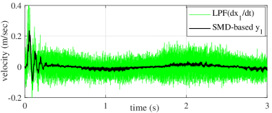
Figure 8: SMD based estimation $y_{1}(t)$ of the relative velocity versus low-pass filtered discrete time derivative of the measured $x_{1}(t)$.

Therefore, the applied scaling factor $\rho=8$ is tuned experimentally so that the estimate $y_{1}(t)$ is sufficiently accurate with respect to $\dot{x}_{1}(t)$. Note that the latter can be computed (for tuning purposes) as a smooth and noise-free signal, since the measured $x_{1}(t)$ fits with $a_{i}\sin(\omega_{i}t)$ for the driven constant amplitude $a_{i}$ and frequency $\omega_{i}$. The driven and measured $x_{1}(t)$ with two limiting angular frequencies $\omega_{i}=\{0.1,\,10\}$ rad/sec where used for tuning the $\rho$-parameter. For highlighting the resulted SMD performance, the $y_{1}(t)$-estimation of the relative velocity is exemplary compared in Figure 8 with the discrete-time differentiated signal $\dot{x}_{1}(t)$ which is additionally low-pass filtered. The low-pass filter (LPF) is designed as a second-order Butterworth filter with the cutoff frequency at 200 Hz. The used $x_{1}(t)$ data are taken from the closed-loop control experiment (cf. section 3.3 below) of a 0.5 Hz sinusoidal motion profile, including the initial transient oscillations of the relative velocity.

3.3 System identification and PD control tuning

The basic linear model (13) of the motion system is identified from the experimentally collected frequency response (FR) data $x_{1}(j\omega)/u(j\omega)$ of the drive. To this end, a closed-loop identification was performed to keep the drive position $x_{1}(t)$ away from the mechanical limits of the operation range, while allowing for a periodic excitation and motion which are both required for FR measurement. In the applied control signal (22), the closed-loop control (here for the identification purposes only) resulted in

$$u(t)=k_{id}(r_{0}-x(t))+a\sin\omega_{i}t.$$

The proportional feedback gain $k_{id}$ was experimentally tuned in order to provide the relative zero position at $r_{0}=6$ mm, which is approximately the half of the operation range.

Figure 9: Experimentally measured FR versus identified model (13).

The constant amplitude $a$ has also been tuned experimentally, so as to allow for a sufficient periodic motion with the set of angular frequencies $\omega_{i}\in[1,\ldots,1000]$ rad/sec. The FR data were collected from the measured steady-sate oscillations at $\omega_{i}$, equidistantly distributed on the logarithmic scale, cf. Figure 9. The FR data were used for the least-squares best-fit of the model (13), while those low-frequency points were taken out form the FR data set where the amplitude response violates the $-20$ dB/dec decrease. Recall that the latter is strictly required for the free integrator of the system plant, cf. Figure 9. The FR identified model parameters are $K=0.0463$ and $\tau=0.0076$. Comparing the measured and identified frequency characteristics in Figure 9 one can recognize that both factors, the gain and dominant time constant, are sufficiently mapped and, therefore, identifiable from the collected data set. At the same time, it becomes apparent that inclusion of an additional (electrical) time constant of the voice-coil motor, which is known from the manufacturer’s data sheet, would only marginally improve the amplitude and phase agreement of the model with the measured FR. From the measured phase response one can recognize much more a rapid (close to exponential) increase of the phase lag, that can be attributed to an overall additional time delay $\theta$, i.e. with the corresponding $\exp(-\theta s)$ transfer characteristics. This can arise from all sensing, actuating, and power amplifying elements in the loop. Obviously, this remarkable reduction in the phase capacity will restrict the overall control gain $\gamma$ and, therefore, the achievable bandwidth.

The reference PD feedback controller, cf. section 2.4, is designed based on the identified linear model (13) and the above analysis of the measured FR of the motion system. Since the differential control part lifts up the phase characteristics of the open-loop, it is sufficient to determine the control gain $\gamma$ with respect to the resulted crossover frequency and the associated phase margin of the measured FR. The determined $\gamma=1000$ leads to the crossover frequency $\omega_{c}=46.3$ rad/sec, for which the phase margin $\pi+\angle\mathrm{FR}(\omega_{c})+\angle\mathrm{PD}(\omega_{c})$ of the measured FR characteristics, and further shaped by the PD controller, results in approximately $\approx 50$ deg, cf. Figure 9. This robust phase margin appears reasonable for the feedback control design, here for taking into account the system uncertainties, differentiation of the system output $x_{1}(t)$, and non-modeled (to say hidden) residual dynamics in the control loop.

3.4 Comparison of PD and OND controllers

Both feedback controllers, the introduced OND (17) and reference PD (19), are experimentally evaluated with one the same output feedback gain $\gamma=1000$. Both are applied (alternately) to the input signal (22). Both are also sharing the same second-order SMD, designed as in section 3.2 for use of $y_{1}(t)$ instead of $x_{2}(t)$, which is not available.

First, two sinusoidal reference trajectories are evaluated, one with 0.5Hz and another one with 2Hz frequency. Both are shown in Figure 10 (a) and (b), correspondingly. It is visible that both controllers have a similar transient response, while the OND control discloses a lower phase lag and reaches better the peaks of a periodic trajectory. At the same time, the OND control tends to a higher initial overshoot, cf. also with state trajectories in Figure 1. This can be explained by a decreasing damping ratio once $|e_{1}|$ is growing.

As next, a relatively flat linear slope trajectory is evaluated as shown in Figure 11. This assumed the controlled motion with a slow constant velocity of $\dot{r}=0.002$ m/sec. One can recognize that the OND control is outperforming the PD one in both following features. (i) It is tracking more uniformly the reference trajectory, i.e. keeping $e_{1}(t)\approx\mathrm{const}$ during the steady-state motion. (ii) It is converging closer to the final reference set value, i.e. having lower $e_{1}(t)$ at $t\rightarrow\infty$ in presence of the unavoidable perturbations $\xi$. Note that the latter can be attributed to e.g. magnetic force ripples of the void-coil motor and Coulomb friction, see e.g. [15] for details, in the drive. The corresponding control values (see Figure 11 (b)) discloses that the OND control is comparable with PD in energy consumption, and has even slightly lower peaking during the transient phase and lower average level at steady-state. Recall that the static bias and jitter are included for both controls, cf. (22). The control error performance of both controllers is further visible in more detail in Figure 11 (c). Here the same measured data from the slope reference experiment is used, but with a longer steady-state phase for better highlighting the $e_{1}(t)$ performance.

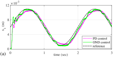
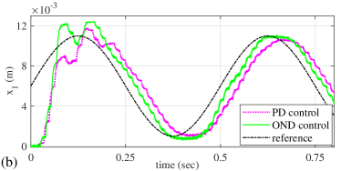
Figure 10: Measured position response of OND and PD controls to the sinusoidal reference trajectory of 0.5Hz in (a) and 2Hz in (b).

Finally, the ability of disturbance rejection is evaluated for both controllers. For this purpose, the step reference was used and, afterwards, the manually inserted disturbance was applied during the steady-state. The disturbance was induced by pressing down the moving body of the drive, cf. Figure 7, thus inducing an external counteracting force which brings the motion control away from the constat set reference position $r(t)=0.01$ m. The applied disturbance was also released manually, thus leading to the not repeatable and not equivalent motion profiles, shown in Figure 12. One can recognize that the OND control behaves more stiff during the step-wise excitations. In the left zoom-in plot, the step response comes even beyond the sensor saturation at $x_{1}=0.012$ m that is, however, recovered after the transient overshot of the OND control. In the right zoom-in plot, one can recognize that the OND control is recovering as fast as the PD control, and comes to the same residual error level after short transients.

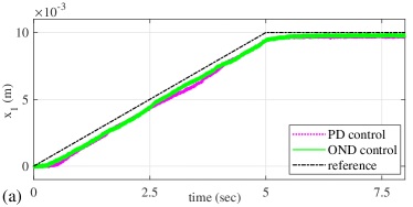
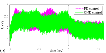
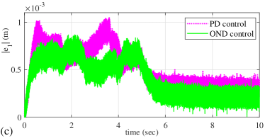
Figure 11: Measured position response of OND and PD controls to the slope reference (a), control value (b), absolute control error (c).

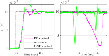
Figure 12: Measured position response of OND and PD controls to the step reference and manually inserted disturbance.

4 CONCLUSIONS

In this paper, we have revised the optimal nonlinear damping (OND) control [14, 13] from a more practical motion control viewpoint. We have extended the admissible plant dynamics to rather realistic motion systems with damping and gain factors and bounded matched perturbations. In the theoretical part, we showed also how an optimal reference PD feedback controller is parameterized by the same feedback gain as the OND control, making both controllers well comparable in a fair benchmark setting. The practical part of the paper introduced and identified the experimental drive, which is based on the voice-coil motor and has a relatively high level of the measurement and process noise. The experimental control evaluation demonstrated that the proposed OND control is outperforming the PD reference control in both, the transient response and residual steady-state error. The OND control proved also to be robust against the essential external disturbances applied to the experimental drive. A significantly faster convergence of the OND control towards zero equilibrium, cf. Figure 5, highlights its advantages in case of a more accurate output position measurement, with the corresponding higher requirements posed on the motion control system. The following possible issues, however, have to be taken into account when applying the OND control. (i) the regularization term $\mu>0$ cannot be arbitrary decreased, especially in presence of the measurement noise. For $|e_{1}|\rightarrow 0$ and non-zero velocities, the control dynamics can lead to some residual chattering, owing to the very small $\mu$ values and alternating sign of $e_{2}$, cf. with eq. (7). (ii) the transient peaking of the OND control can be higher than of the PD control (cf. section 3.4), which can provide additional challenges for certain type of the applications. Despite the above mentioned shortcomings, it is believed that the OND control represents an interesting alternative to the conventional PD type controllers, also with a potential for further developments and extensions, like for example by an integral control action.

References

- Anderson and Spong [1988] Anderson, R.J., Spong, M.W., 1988. Hybrid impedance control of robotic manipulators. IEEE Journal on Robotics and Automation 4, 549–556.
- Demidovich [1967] Demidovich, B., 1967. Lectures on the mathematical theory of stability. Nauka, Moscow.
- Dietrich et al. [2021] Dietrich, A., Wu, X., Bussmann, K., Harder, M., Iskandar, M., Englsberger, J., Ott, C., Albu-Schäffer, A., 2021. Practical consequences of inertia shaping for interaction and tracking in robot control. Control Engineering Practice 114, 104875.
- Franklin et al. [2015] Franklin, G., Powell, J., Emami-Naeini, A., 2015. Feedback Control of Dynamic Systems. Seventh ed., Pearson.
- Heertjes et al. [2015] Heertjes, M.F., Van der Velden, B., Oomen, T., 2015. Constrained iterative feedback tuning for robust control of a wafer stage system. IEEE Transactions on Control Systems Technology 24, 56–66.
- Iwasaki et al. [2012] Iwasaki, M., Seki, K., Maeda, Y., 2012. High-precision motion control techniques: A promising approach to improving motion performance. IEEE Industrial Electronics Magazine 6, 32–40.
- Kelly and Carelli [1996] Kelly, R., Carelli, R., 1996. A class of nonlinear PD-type controllers for robot manipulators. Journal of Robot. Syst. 13, 793–802.
- Levant [1998] Levant, A., 1998. Robust exact differentiation via sliding mode technique. Automatica 34, 379–384.
- Moreno [2012] Moreno, J.A., 2012. Lyapunov function for Levant’s second order differentiator, in: IEEE 51st conference on decision and control (CDC’12), pp. 6448–6453.
- Pavlov et al. [2004] Pavlov, A., Pogromsky, A., van de Wouw, N., Nijmeijer, H., 2004. Convergent dynamics, a tribute to Boris Pavlovich Demidovich. Systems & Control Letters 52, 257–261.
- Rao and Bernstein [2001] Rao, V.G., Bernstein, D.S., 2001. Naive control of the double integrator. IEEE Control Systems Magazine 21, 86–97.
- Reichhartinger et al. [2017] Reichhartinger, M., Spurgeon, S., Forstinger, M., Wipfler, M., 2017. A robust exact differentiator toolbox for Matlab®/Simulink®. IFAC-PapersOnLine 50, 1711–1716.
- Ruderman [2021a] Ruderman, M., 2021a. Convergent dynamics of optimal nonlinear damping control. IFAC-PapersOnLine 54, 141–144.
- Ruderman [2021b] Ruderman, M., 2021b. Optimal nonlinear damping control of second-order systems. Journal of The Franklin Institute 358, 4292–4302.
- Ruderman and Iwasaki [2015] Ruderman, M., Iwasaki, M., 2015. Observer of nonlinear friction dynamics for motion control. IEEE Transactions on Industrial Electronics 62, 5941–5949.
- Shahruz et al. [1992] Shahruz, S., Langari, G., Tomizuka, M., 1992. Optimal damping ratio for linear second-order systems. Journal of optimization theory and applications 73, 563–576.
- Shtessel et al. [2014] Shtessel, Y., Edwards, C., Fridman, L., Levant, A., et al., 2014. Sliding mode control and observation. Springer.
- Tomei [1991] Tomei, P., 1991. A simple PD controller for robots with elastic joints. IEEE Transactions on automatic control 36, 1208–1213.
- Xu et al. [1995] Xu, Y., Hollerbach, J.M., Ma, D., 1995. A nonlinear PD controller for force and contact transient control. IEEE Control Systems Magazine 15, 15–21.