An $hp$-version interior penalty discontinuous Galerkin method for the quad-curl eigenvalue problem

Abstract

An $hp$-version interior penalty discontinuous Galerkin (IPDG) method under nonconforming meshes is proposed to solve the quad-curl eigenvalue problem. We prove well-posedness of the numerical scheme for the quad-curl equation and then derive an error estimate in a mesh-dependent norm, which is optimal with respect to $h$ but has different p-version error bounds under conforming and nonconforming tetrahedron meshes. The $hp$-version discrete compactness of the DG space is established for the convergence proof. The performance of the method is demonstrated by numerical experiments using conforming/nonconforming meshes and $h$-version/$p$-version refinement. The optimal $h$-version convergence rate and the exponential $p$-version convergence rate are observed.

1 Introduction

The quad-curl eigenvalue problem is important in inverse electromagnetic scattering theory of inhomogeneous media [15, 38, 49] and magnetohydrodynamics equations [54]. As a classic electromagnetic model, the Maxwell eigenvalue problem is a hot topic in the field of numerical mathematics and computational electromagnetism (see, e.g., [2, 8, 10, 11, 12, 13, 21, 31, 36, 37, 39, 46, 47]). In recent years, the numerical treatment of the quad-curl equation and its associated eigenvalue problem has attracted the attention of scientific community. Some early works include a nonconforming element method by Zheng et al. [54] and an $h$-version IPDG method by Hong et al. [32], respectively, for the quad-curl equation. Chen et al. [18] and Sun et al. [50] further established its new a-priori error estimates and multigrid method, respectively. Sun et al. [49] also proposed an $h$-version weak Galerkin method for the quad-curl equation. Sun [48] and Zhang [55] studied its mixed element methods, respectively. Brenner et al. [14] proposed its Lagrange finite element methods on planar domains. More recently Zhang and Hu et al. [53, 29, 30] proposed several families of ${\bf H}(\mathrm{curl}^{2})$-conforming finite elements in both two and three dimensions. A-priori and a-posteriori error estimates for the quad-curl eigenvalue problem were further developed in [52]. The ${\bf H}(\mathrm{curl}^{2})$-conforming virtual element methods [57] and the decoupled finite element method [17] were also proposed.

The $hp$ finite element methods are popular in scientific computing due to its flexibility and high accuracy. DG methods provide general framework for $hp$-adaptivity as they employ the discontinuous finite element spaces, giving great flexibility in the design of meshes and polynomial bases. For the overview of the historical development of $hp$-version DG methods, we refer to, e.g., articles [1, 5], monographs [22, 44] and the references therein. For the second-order elliptic problem and the biharmonic problem, a considerable number of works on $hp$-version IPDG methods were done, cf. [33, 40, 41, 51, 26, 27, 25, 35, 43].

However, to the best of our knowledge, the research work on the $hp$-version DG methods for the quad-curl equation and its eigenvalue problem cannot be found in the existing literatures. This paper aims to fill this gap. We propose an $hp$-version IPDG method with two interior penalty parameters to solve the quad-curl equation and associated eigenvalue problem. The $hp$-version error estimates for the DG solution of the quad-curl equation (without div-free constraint) are established under the assumption that the exact solution $\bm{w}\in{\bf H}^{3}(\Omega)$ and $\mathrm{curl}^{3}\bm{w}\in{\bf H}^{1/2+\delta}(\Omega)$. To bound the error of the IPDG method for the eigenvalue problem, we analyze the $hp$-version DG discretization of the quad-curl equation with div-free constraint. A discrete poincáre inequality in the discrete div-free space is established to guarantee the well-posedness of the DG discretization scheme. Then $hp$-version discrete compactness on the discrete div-free space is established to prove the unform convergence of discrete solution operators. Finally, we use the well-known Babus̆ka-Osborn theory [3] to prove the convergence of the IPDG method for the quad-curl eigenvalue problem. The a priori error bound of the DG eigenvalues is optimal in $h$ on both conforming and nonconforming meshes, and suboptimal in $p$ by 3 order on nonconforming simplex mesh and by 2 order on conforming simplex mesh.

This paper is structured as follows. In Section 2, an $hp$-version IPDG scheme is given for the quad-curl equation without $div$-free condition. In Section 3, we will discuss the stability of the IPDG scheme and its a-priori error estimates in DG norm under conforming/nonconforming mesh. An IPDG scheme for the quad-curl eigenvalue problem is proposed in Section 4. The discrete poincáre inequality and discrete compactness of discrete $div$-free space are established. The error bound for IPDG eigenvalues and the error estimates of eigenfunctions in low norms will follow. In the end of this paper, we present several numerical examples to validate the efficiency of our methods under both $h$-refinement and $p$-refinement modes.

Throughout this paper, we use the symbol $a\lesssim b$ and $a\gtrsim b$ to mean that $a\leq Cb$ and $a\geq Cb$ respectivley, where $C$ denotes a positive constant independent of mesh parameters and polynomial degrees and may not be the same in different places.

2 An $hp$-version IPDG method for the quad-curl problem

Consider the quad-curl problem

$$\mathrm{curl}^{4}\bm{w}+\bm{w} =\bm{f}~{}~{}~{}in~{}\Omega,$$ (2.1)

$$\mathrm{curl}\bm{w}\times\bm{n} =0~{}~{}~{}on~{}\partial\Omega,$$ (2.2)

$$\bm{w}\times\bm{n} =0~{}~{}~{}on~{}\partial\Omega,$$ (2.3)

where $\Omega$ is a bounded simply-connected Lipschitz polyhedron domain in $\mathbb{R}^{d}$($d=2,3$), and ${\bf n}$ is the unit outward normal to $\partial\Omega$.

We adopt the following function space

$$\mathbf{H}(\mathrm{curl}^{s},\Omega):=\{\bm{v}\in\mathbf{L}^{2}(\Omega):\mathrm{curl}^{j}\bm{v}\in\mathbf{L}^{2}(\Omega),1\leq j\leq s\}$$

equipped with the norm $\|\cdot\|_{s,\mathrm{curl}}$ and

$$\mathbf{H}_{0}(\mathrm{curl}^{2},\Omega):=\{\bm{v}\in\mathbf{L}^{2}(\Omega):\mathrm{curl}^{j}\bm{v}\in\mathbf{L}^{2}(\Omega),\mathrm{curl}^{j-1}\bm{v}\times\bm{n}|_{\partial\Omega}=0,1\leq j\leq 2\}$$

The weak form of (2.1)-(2.3) is to find $\bm{w}\in\mathbf{H}_{0}(\mathrm{curl}^{2},\Omega)$ such that

$$a(\bm{w},\mathbf{v})=(\bm{f},\mathbf{v}),~{}~{}\forall\mathbf{v}\in\mathbf{H}_{0}(\mathrm{curl}^{2},\Omega),$$ (2.4)

where

$$a(\bm{w},\mathbf{v})=(\mathrm{curl}^{2}\bm{w},\mathrm{curl}^{2}\bm{v})+(\bm{w},\bm{v}).$$

We consider the shape regular and affine meshes $\mathcal{T}_{h}=\{K\}$ that partition the domain $\Omega$ into tetrahedra in $\mathbb{R}^{3}$ (or triangles in $\mathbb{R}^{2}$), and introduce the finite element space

$${\bf V}_{h} =\{\bm{v}_{h}|_{K}\in P(K),K\in\mathcal{T}_{h},p_{K}\geq 2\}.$$ (2.5)

where $P(K)=(P_{p_{K}})^{d}$ with the polynomial space of total $\text{degree}\leq p_{K}$. Let $h=\max_{K\in\mathcal{T}_{h}}h_{K}$ and $p=\min_{K\in\mathcal{T}_{h}}p_{K}$. Let $\mathcal{E}^{0}_{h}$ and $\mathcal{E}^{\partial}_{h}$ be respectively the set of internal faces and the set of boundary faces of partition $\mathcal{T}_{h}$, $\mathcal{E}_{h}:=\mathcal{E}^{0}_{h}\cup\mathcal{E}^{\partial}_{h}$, $f\in\mathcal{E}^{0}_{h}$ be the interface of two adjacent elements $K^{\pm}$, and $\bm{n}^{\pm}$ be the unit outward normal vector of the face $f$ associated with $K^{\pm}$. We use $h_{f}:=\max(h_{K^{+}},h_{K^{-}})$ and $p_{f}:=\min(p_{K^{+}},p_{K^{-}})$ to represent the maximum diameter of the circumcircle and the maximum polynomial degree of the elements sharing the face $f$, respectively. We denote by $\bm{v}^{\pm}=(\bm{v}|_{K^{\pm}})|_{f}$ and introduce three notations as follows:

$$\llbracket\bm{v}\rrbracket =\bm{v}^{+}\times\bm{n}^{+}+\bm{v}^{-}\times\bm{n}^{-},~{}~{}\llbracket\mathrm{curl}\bm{v}\rrbracket =\mathrm{curl}\bm{v}^{+}\times\bm{n}^{+}+\mathrm{curl}\bm{v}^{-}\times\bm{n}^{-},~{}~{}\{\mathrm{curl}^{2}\bm{v}\} =(\mathrm{curl}^{2}\bm{v}^{+}+\mathrm{curl}^{2}\bm{v}^{-})/2.$$

If $f\in\mathcal{E}^{\partial}_{h}$, we define $\llbracket\bm{v}\rrbracket$, $\llbracket\mathrm{curl}\bm{v}\rrbracket$ and $\{\mathrm{curl}^{2}\bm{v}\}$ on $f$, respectively, as follows:

$$\llbracket\bm{v}\rrbracket=\bm{v}\times\bm{n},~{}~{}\llbracket\mathrm{curl}\bm{v}\rrbracket=\mathrm{curl}\bm{v}\times\bm{n},~{}~{}\{\mathrm{curl}^{2}\bm{v}\}=\mathrm{curl}^{2}\bm{v}.$$

Pick up any $\bm{v}_{h}$ in ${\bf V}_{h}$. For any $K\in\mathcal{T}_{h}$, by using Green’s formula we have

$$\int_{K}\bm{f}\cdot\bm{v}_{h} =\int_{\partial K}\mathrm{curl}^{3}\bm{w}\cdot\bm{v}_{h}\times\bm{n}ds+\int_{K}\mathrm{curl}^{2}\bm{w}\cdot\mathrm{curl}^{2}\bm{v}_{h}dx+\int_{K}\bm{w}\cdot\bm{v}_{h}dx$$

$$~{}~{}~{}+\int_{\partial K}\mathrm{curl}^{2}\bm{w}\cdot(\mathrm{curl}\bm{v}_{h}\times\bm{n})ds.$$ (2.6)

This infers that

$$\int_{\Omega}\bm{f}\cdot\bm{v}_{h}dx =\int_{\Omega}\mathrm{curl}_{h}^{2}\bm{w}\cdot\mathrm{curl}_{h}^{2}\bm{v}_{h}dx+\int_{f\in\mathcal{E}_{h}}\mathrm{curl}^{3}\bm{w}\cdot\llbracket\bm{v}_{h}\rrbracket ds+\int_{\Omega}\bm{w}\cdot\bm{v}_{h}dx$$

$$~{}~{}~{}+\int_{f\in\mathcal{E}_{h}}\mathrm{curl}^{2}\bm{w}\cdot\llbracket\mathrm{curl}\bm{v}_{h}\rrbracket ds$$ (2.7)

whose right-hand side can be rewritten as the bilinear form

$$a_{h}(\bm{w},\bm{v}_{h}) =\int_{\Omega}\mathrm{curl}_{h}^{2}\bm{w}\cdot\mathrm{curl}_{h}^{2}\bm{v}_{h}dx+\int_{\Omega}\bm{w}\cdot\bm{v}_{h}dx$$

$$~{}~{}~{}+\int_{f\in\mathcal{E}_{h}}\{\mathrm{curl}^{3}\bm{w}\}\cdot\llbracket\bm{v}_{h}\rrbracket ds+\int_{f\in\mathcal{E}_{h}}\{\mathrm{curl}^{2}\bm{w}\}\cdot\llbracket\mathrm{curl}\bm{v}_{h}\rrbracket ds$$

$$~{}~{}~{}+\int_{f\in\mathcal{E}_{h}}\{\mathrm{curl}^{3}\bm{v}_{h}\}\cdot\llbracket\bm{w}\rrbracket ds+\int_{f\in\mathcal{E}_{h}}\{\mathrm{curl}^{2}\bm{v}_{h}\}\cdot\llbracket\mathrm{curl}\bm{w}\rrbracket ds$$

$$~{}~{}~{}+\int_{f\in\mathcal{E}_{h}}\frac{\eta_{1}p^{2}_{f}}{h_{f}}\llbracket\mathrm{curl}\bm{v}_{h}\rrbracket\cdot\llbracket\mathrm{curl}\bm{w}\rrbracket ds+\int_{f\in\mathcal{E}_{h}}\frac{\eta_{2}p^{6}_{f}}{h_{f}^{3}}\llbracket\bm{v}_{h}\rrbracket\cdot\llbracket\bm{w}\rrbracket ds$$ (2.8)

where we have used the jump $\llbracket\mathrm{curl}\bm{w}\rrbracket$ and $\llbracket\bm{w}\rrbracket$ vanishes across faces $f$ and $\eta_{1}$ and $\eta_{2}$ are two positive constant to be determined. Finally we reach at the following relation

$$a_{h}(\bm{w},\bm{v}_{h}) =(\bm{f},\bm{v}_{h}),\quad\forall\bm{v}_{h}\in{\bf V}_{h}.$$ (2.9)

Hence the IPDG discretization of (2.5) is to find $\bm{w}_{h}\in{\bf V}_{h}$ such that

$$a_{h}(\bm{w}_{h},\bm{v}_{h}) =(\bm{f},\bm{v}_{h}),\quad\forall\bm{v}_{h}\in{\bf V}_{h}.$$ (2.10)

The above two equalities give the following Galerkin orthogonality

$$a_{h}(\bm{w}_{h}-\bm{w},\bm{v}_{h}) =0,\quad\forall\bm{v}_{h}\in{\bf V}_{h}.$$ (2.11)

Lemma 2.0 (Lemma 4.5 in [4]).

There are linear continuous operators $\Pi_{p}^{K}:{\bf H}^{s}(K)\to P(K)$ such that for $\bm{v}\in{\bf H}^{s}(K)$

$$\|\bm{v}-\Pi_{p}^{K}\bm{v}\|_{q,K} \lesssim h_{K}^{\min(p_{K}+1,s)-q}p_{K}^{q-s}\|\bm{v}\|_{s,K},~{}0\leq q\leq s,$$ (2.12)

Let $\bm{v}\in{\bf V}_{h}$ be equipped with the following norm and semi-norm

$$||\bm{v}||_{h}^{2} :=\sum_{K\in\mathcal{T}_{h}}\left(\|\mathrm{curl}^{2}\bm{v}\|_{0,K}^{2}+\|\bm{v}\|_{0,K}^{2}\right)+\sum_{\bm{f}\in\mathcal{E}_{h}}\left(h_{f}^{-3}p_{f}^{6}\|\llbracket\bm{v}\rrbracket\|_{0,f}^{2}\right)$$

$$~{}~{}~{}+\sum_{\bm{f}\in\mathcal{E}_{h}}\left(h_{f}^{3}p_{f}^{-6}\|\{\mathrm{curl}^{3}\bm{v}\}\|_{0,f}^{2}+h_{f}p_{f}^{-2}\|\{\mathrm{curl}^{2}\bm{v}\}\|_{0,f}^{2}+h_{f}^{-1}p_{f}^{2}\|\llbracket\mathrm{curl}\bm{v}\rrbracket\|_{0,f}^{2}\right),$$ (2.13)

$$|\bm{v}|_{h}^{2} :=\|\bm{v}\|_{h}^{2}-\|\bm{v}\|^{2}.$$ (2.14)

Next we shall discuss the well-posedness of the discrete variational problem. It is obvious that the bilinear form $a_{h}(\cdot,\cdot)$ is bounded with respect to the norm $\|\cdot\|_{h}$ in ${\bf V}_{h}+{\bf H}_{0}(\mathrm{curl}^{2},\Omega)\cap\{\bm{v}:\sum_{j=0}^{3}\|\mathrm{curl}^{j}\bm{v}\|_{1/2+\sigma,\Omega}<\infty\}$ with $\sigma>0$.

3 Error estimate in DG-norm

Lemma 3.0 (Lemma 6.1 in [28]).

For any polynomial $\bm{v}\in{\bf P}(K)$, there holds

$$\|\bm{v}\|_{0,\partial K}\lesssim h_{K}^{-1/2}p_{K}\|\bm{v}\|_{0,K}~{}\text{and}~{}|\bm{v}|_{1,K}\lesssim h_{K}^{-1}p_{K}^{2}\|\bm{v}\|_{0,K}.$$ (3.1)

The following theorem shows the coerciveness of $a_{h}(\cdot,\cdot)$ in ${\bf V}_{h}$, which guarantees the well-posedness of the discrete problem (2.10).

Theorem 3.1.

For sufficiently large $\eta_{1}$ and $\eta_{2}$, we have

$$a_{h}(\bm{v},\bm{v})\gtrsim\|\bm{v}\|_{h}^{2},~{}\forall\bm{v}\in{\bf V}_{h}.$$ (3.2)

Proof.

Let us pick up any $\bm{v}\in{\bf V}_{h}$ we deduce

$$a_{h}(\bm{v},\bm{v}) \geq\sum_{K\in\mathcal{T}_{h}}\left(\|\mathrm{curl}^{2}\bm{v}\|_{0,K}^{2}+\|\bm{v}\|_{0,K}^{2}\right)+\sum_{\bm{f}\in\mathcal{E}_{h}}\left(\eta_{1}h_{f}p^{2}_{f}\|\llbracket\mathrm{curl}\bm{v}\rrbracket\|_{0,f}^{2}+\eta_{2}h_{f}^{-3}p^{6}_{f}\|\llbracket\bm{v}\rrbracket\|_{0,f}^{2}\right)$$

$$~{}~{}~{}-\rho_{1}^{-1}\sum_{\bm{f}\in\mathcal{E}_{h}}h_{f}p^{-2}_{f}\|\{\mathrm{curl}^{2}\bm{v}\}\|_{0,f}^{2}-\rho_{1}\sum_{\bm{f}\in\mathcal{E}_{h}}h_{f}^{-1}p^{2}_{f}\|\llbracket\mathrm{curl}\bm{v}\rrbracket\|_{0,f}^{2}$$

$$~{}~{}~{}-\rho_{2}^{-1}\sum_{\bm{f}\in\mathcal{E}_{h}}h_{f}^{3}p^{-6}_{f}\|\{\mathrm{curl}^{3}\bm{v}\}\|_{0,f}^{2}-\rho_{2}\sum_{\bm{f}\in\mathcal{E}_{h}}h_{f}^{-3}p^{6}_{f}\|\llbracket\bm{v}\rrbracket\|_{0,f}^{2}$$ (3.3)

with $\rho_{1}$ and $\rho_{2}$ to be determined later. Using trace theorem and inverse estimate in Lemma 3.1, we have for $f=\overline{K_{1}}\cap\overline{K_{2}}$

$$h_{f}p_{f}^{-2}\|\{\mathrm{curl}^{2}\bm{v}\}\|_{0,f}^{2} \leq 0.5C_{1}\|\mathrm{curl}^{2}\bm{v}\|_{0,K_{1}\cup K_{2}}^{2},$$ (3.4)

$$h_{f}^{3}p_{f}^{-6}\|\{\mathrm{curl}^{3}\bm{v}\}\|_{0,f}^{2} \leq C_{2}h_{f}p_{f}^{-2}\|\{\mathrm{curl}^{2}\bm{v}\}\|_{0,f}^{2}\leq 0.5C_{2}C_{1}\|\mathrm{curl}^{2}\bm{v}\|_{0,K_{1}\cup K_{2}}^{2}.$$ (3.5)

Then we deduce

$$a_{h}(\bm{v},\bm{v}) \geq\sum_{K\in\mathcal{T}_{h}}\left(\|\mathrm{curl}^{2}\bm{v}\|_{0,K}^{2}+\|\bm{v}\|_{0,K}^{2}\right)+\sum_{\bm{f}\in\mathcal{E}_{h}}\left(\eta_{1}h_{f}^{-1}p^{2}_{f}\|\llbracket\mathrm{curl}\bm{v}\rrbracket\|_{0,f}^{2}+\eta_{2}h_{f}^{-3}p^{6}_{f}\|\llbracket\bm{v}\rrbracket\|_{0,f}^{2}\right)$$

$$~{}~{}~{}-2\rho_{1}^{-1}C_{1}\sum_{K\in\mathcal{T}_{h}}\|\mathrm{curl}^{2}\bm{v}\|_{0,K}^{2}-\rho_{1}\sum_{\bm{f}\in\mathcal{E}_{h}}h_{f}^{-1}p^{2}_{f}\|\llbracket\mathrm{curl}\bm{v}\rrbracket\|_{0,f}^{2}$$

$$~{}~{}~{}-2\rho_{2}^{-1}C_{1}C_{2}\sum_{K\in\mathcal{T}_{h}}\|\mathrm{curl}^{2}\bm{v}\|_{0,K}^{2}-\rho_{2}\sum_{\bm{f}\in\mathcal{E}_{h}}h_{f}^{-3}p^{6}_{f}\|\llbracket\bm{v}\rrbracket\|_{0,f}^{2}.$$ (3.6)

Hence

$$a_{h}(\bm{v},\bm{v}) \geq\sum_{K\in\mathcal{T}_{h}}\left((1-2\rho_{1}^{-1}C_{1}-2\rho_{2}^{-1}C_{1}C_{2})\|\mathrm{curl}^{2}\bm{v}\|_{0,K}^{2}+\|\bm{v}\|_{0,K}^{2}\right)$$

$$~{}~{}~{}+\sum_{\bm{f}\in\mathcal{E}_{h}}\left(h_{f}^{-1}(\eta_{1}-\rho_{1})p_{f}^{2}\|\llbracket\mathrm{curl}\bm{v}\rrbracket\|_{0,f}^{2}+(\eta_{2}-\rho_{2})h_{f}^{-3}p_{f}^{6}\|\llbracket\bm{v}\rrbracket\|_{0,f}^{2}\right)$$ (3.7)

Choose the large $\rho_{1}$, $\rho_{2}$, $\eta_{1}$ and $\eta_{2}$ such that $2\rho_{1}^{-1}C_{1}+2\rho_{2}^{-1}C_{1}C_{2}<1$, $\eta_{1}>\rho_{1}$ and $\eta_{2}>\rho_{2}$. Finally the inequality (3) together with (3.4) yields the conclusion. ∎

In the following theorem, we prove the error estimate of the discrete problem (2.10) by establishing the interpolation error estimates in DG-norm.

Theorem 3.2.

Assume that $\{\mathcal{T}_{h}\}$ is a family of nonconforming meshes. Let $\bm{w}\in{\bf H}_{0}(\mathrm{curl}^{2},\Omega)$ and $A_{K}(\bm{w})<\infty$ for any $K\in\mathcal{T}_{h}$ then

$$\|\bm{w}-\bm{w}_{h}\|_{h} \lesssim\left(\sum_{K\in\mathcal{T}_{h}}(h_{K}^{\min(p_{K}+1,s_{K})-2}p_{K}^{3.5-s_{K}}A_{K}(\bm{w}))^{2}\right)^{1/2},\quad p:={\min_{K\in\mathcal{T}_{h}}p_{K}}\geq 2$$ (3.8)

where $A_{K}(\bm{w}):=\|\bm{w}\|_{s_{K},K}$ if $\|\bm{w}\|_{s_{K},K}<\infty$ for $s_{K}\geq 4$, otherwise $A_{K}(\bm{w}):=\|\bm{w}\|_{3,K}+\|\mathrm{curl}^{3}\bm{w}\|_{1/2+\delta,K}$ $(\delta>0)$ and $s_{K}=3$.

Proof.

Let $\Pi_{p}$ be the global projection operator which equals $\Pi_{p}^{K}$ on $K$. First of all we shall prove

$$\|\bm{w}-\Pi_{p}\bm{w}\|_{h} \lesssim\left(\sum_{K\in\mathcal{T}_{h}}(h_{K}^{\min(p_{K}+1,s_{K})-2}p_{K}^{3.5-s_{K}}A_{K}(\bm{w})\right)^{1/2},\quad p_{K},s_{K}\geq 2.$$ (3.9)

Let us denote $E_{h}(\bm{w})=\bm{w}-\Pi_{p}\bm{w}$ then

$$\|E_{h}(\bm{w})\|_{h}^{2} \lesssim\sum_{K\in\mathcal{T}_{h}}\left(\|\mathrm{curl}^{2}E_{h}(\bm{w})\|_{0,K}^{2}+\|E_{h}(\bm{w})\|_{0,K}^{2}\right)+\sum_{\bm{f}\in\mathcal{E}_{h}}h_{f}^{3}p_{f}^{-6}\|\{\mathrm{curl}^{3}E_{h}(\bm{w})\}\|_{0,f}^{2}$$

$$~{}~{}~{}+\sum_{\bm{f}\in\mathcal{E}_{h}}\left(p_{f}^{6}h_{f}^{-3}\|\llbracket E_{h}(\bm{w})\rrbracket\|_{0,f}^{2}+p_{f}^{2}h_{f}^{-1}\|\llbracket\mathrm{curl}E_{h}(\bm{w})\rrbracket\|_{0,f}^{2}+p_{f}^{-2}h_{f}\|\{\mathrm{curl}^{2}E_{h}(\bm{w})\}\|_{0,f}^{2}\right)$$

$$:=I_{1}+I_{2}+I_{3}.$$

We first estimate $I_{1}$. Using the error estimate of $\Pi^{K}_{p}$ in Lemma 2.1, we have

$$\|E_{h}(\bm{w})\|_{0,K}+\|\mathrm{curl}^{2}E_{h}(\bm{w})\|_{0,K}\lesssim h_{K}^{\min(p_{K}+1,s_{K})-2}p_{K}^{2-s_{K}}\|\bm{w}\|_{s_{K},K}.$$

Let $f=\overline{K}_{1}\cap\overline{K}_{2}$ and $s_{f}:=\min(s_{K_{1}},s_{K_{2}})$. For $p_{f}\geq 3$ we have from Lemma 2.1

$$|\mathrm{curl}^{3}E_{h}(\bm{w})|_{1,K_{1}\cup K_{2}}+h_{f}^{-1}p_{f}|\mathrm{curl}^{3}E_{h}(\bm{w})|_{0,K_{1}\cup K_{2}}\lesssim h_{f}^{\min(p_{f}+1,s_{f})-4}p_{f}^{4-s_{f}}\|\bm{w}\|_{s_{f},K_{1}\cup K_{2}}.$$

Then we estimate $I_{2}$: For $p_{f}\geq 2$ we have for $i=1,2$

$$\|\mathrm{curl}^{3}E_{h}(\bm{w})|_{K_{i}}\|_{0,f}^{2}=\|\mathrm{curl}^{3}\bm{w}|_{K_{i}}\|_{0,f}^{2}\lesssim\|\mathrm{curl}^{3}\bm{w}\|_{1/2+\delta,K_{1}\cup K_{2}}^{2}$$

while for $p_{f}\geq 3$ from Lemma A.3 in [45] we have for $i=1,2$

$$\|\mathrm{curl}^{3}E_{h}(\bm{w})|_{K_{i}}\|_{0,f} \lesssim h_{f}^{-1/2}\|\mathrm{curl}^{3}E_{h}(\bm{w})\|_{0,K_{1}\cup K_{2}}+(\|\mathrm{curl}^{3}E_{h}(\bm{w})\|_{0,K_{1}\cup K_{2}}|\mathrm{curl}^{3}E_{h}(\bm{w})|_{1,K_{1}\cup K_{2}})^{1/2}$$

$$\lesssim(h_{f}^{\min(p_{f}+1,s_{f})-3.5}p_{f}^{3-s_{f}}+h_{f}^{\min(p_{f}+1,s_{f})-3.5}p_{f}^{3.5-s_{f}})\|\bm{w}\|_{s_{f},K_{1}\cup K_{2}}$$

$$\lesssim h_{f}^{\min(p_{f}+1,s_{f})-3.5}p_{f}^{3.5-s_{f}}\|\bm{w}\|_{s_{f},K_{1}\cup K_{2}}.$$

We can estimate $I_{3}$ similarly:

$$\|E_{h}(\bm{w})|_{K_{i}}\|_{0,f}+h_{f}p_{f}^{-1}\|\mathrm{curl}(E_{h}(\bm{w}))|_{K_{i}}\|_{0,f}+h_{f}^{2}p_{f}^{-2}\|\mathrm{curl}^{2}(E_{h}(\bm{w}))|_{K_{i}}\|_{0,f}$$

$$~{}~{}~{}\lesssim h_{f}^{\min(p+1,s_{f})-0.5}p_{f}^{0.5-s_{f}}\|\bm{w}\|_{s_{f},K_{1}\cup K_{2}}\text{for $i=1,2$}.$$ (3.10)

Hence we have proved (3.9). Using (2.11) and Theorem 3.1 we have

$$\|\bm{w}_{h}-\bm{v}_{h}\|_{h}^{2}\lesssim a_{h}(\bm{w}_{h}-\bm{v}_{h},\bm{w}-\bm{v}_{h})\lesssim\|\bm{w}_{h}-\bm{v}_{h}\|_{h}\|\bm{w}-\bm{v}_{h}\|_{h},\quad\forall\bm{v}_{h}\in{{\bf V}}_{h}.$$

Then

$$\|\bm{w}-\bm{w}_{h}\|_{h}\lesssim\inf_{\bm{v}_{h}\in{{\bf V}}_{h}}\|\bm{w}-\bm{v}_{h}\|_{h}.$$ (3.11)

This together with (3.9) yields the conclusion. ∎

Remark 3.1.

The error estimate (3.9) on the general polygonal $(d=2)$ or polyhedral $(d=3)$ meshes can be proved by using a triangle or a tetrahedron to cover the polygonal or polyhedral element, like the way in Lemma 23 in [16] or Lemma 4.12 in [24].

Remark 3.2.

The convergence rate is optimal with respect to $h$ but the convergence rate in polynomial degree $p$ is not optimal under nonconforming mesh. The convergence rate can be improved under conforming meshes. The utilization of the $H^{1}$-conforming element interpolation in [4] can yield the following theorem.

Theorem 3.3.

Assume that $\{\mathcal{T}_{h}\}$ is a family of conforming meshes. Let $\bm{w}\in{\bf H}_{0}(\mathrm{curl}^{2},\Omega)$ and $A_{\Omega}(\bm{w}):=(\sum_{K\in\mathcal{T}_{h}}A_{K}(\bm{w})^{2})^{1/2}<\infty$ with $\min_{K\in\mathcal{T}_{h}}s_{K}:=s$ then

$$||\bm{w}-\bm{w}_{h}||_{h} \lesssim h^{\min(p+1,s)-2}p^{3-s}A_{\Omega}(\bm{w}),\quad p\geq 2.$$ (3.12)

Proof.

Let $Q_{h}$ be the $C^{0}$-conforming finite element space defined in [4] with the polynomial degree $p$ and the mesh size $h$. There is a projection $P_{h}:{\bf H}^{1}(\Omega)\to Q_{h}\times Q_{h}$ (see Theorem 4.8 in [4]) such that

$$\|P_{h}\bm{v}-\bm{v}\|_{1,\Omega}\lesssim h^{\min(p+1,l)-1}p^{1-l}\|\bm{v}\|_{l,\Omega},\quad p,l\geq 1.$$ (3.13)

Since

$$|\mathrm{curl}(P_{h}\bm{w}-\bm{w})|_{1,K} \leq|\mathrm{curl}P_{h}\bm{w}-P_{h}\mathrm{curl}\bm{w}|_{1,K}+|P_{h}\mathrm{curl}\bm{w}-\mathrm{curl}\bm{w}|_{1,K}$$

$$\lesssim p_{K}^{2}h_{K}^{-1}\|\mathrm{curl}P_{h}\bm{w}-\mathrm{curl}\bm{w}+\mathrm{curl}\bm{w}-P_{h}\mathrm{curl}\bm{w}\|_{0,K}+\|P_{h}\mathrm{curl}\bm{w}-\mathrm{curl}\bm{w}\|_{1,K},$$

we have

$$\left(\sum_{K\in\mathcal{T}_{h}}|\mathrm{curl}(P_{h}\bm{w}-\bm{w})|_{1,K}^{2}\right)^{1/2} \lesssim h^{\min(p+1,s)-2}p^{3-s}\|\bm{w}\|_{s,\Omega}.$$ (3.14)

Similarly as above, we have

$$\left(\sum_{K\in\mathcal{T}_{h}}\|\mathrm{curl}^{2}(P_{h}\bm{w}-\bm{w})\|_{1,K}^{2}+h_{K}^{2}p_{K}^{-4}\|\mathrm{curl}^{3}(P_{h}\bm{w}-\bm{w})\|_{1,K}^{2}\right)^{1/2}\lesssim h^{\min(p+1,s)-3}p^{5-s}A_{\Omega}(\bm{w}).$$ (3.15)

Denoted by $\widetilde{E}_{h}(\bm{w}):=P_{h}\bm{w}-\bm{w}$, since for $i=1,2$

$$\|\mathrm{curl}^{2}\widetilde{E}_{h}(\bm{w})|_{K_{i}}\|_{0,f} \lesssim h_{f}^{-1/2}\|\mathrm{curl}^{2}\widetilde{E}_{h}(\bm{w})\|_{0,K_{1}\cup K_{2}}+(\|\mathrm{curl}^{2}\widetilde{E}_{h}(\bm{w})\|_{0,K_{1}\cup K_{2}}|\mathrm{curl}^{2}\widetilde{E}_{h}(\bm{w})|_{1,K_{1}\cup K_{2}})^{1/2}$$

we have

$$\left(\sum_{\bm{f}\in\mathcal{E}_{h}}\|\{\mathrm{curl}^{2}\widetilde{E}_{h}(\bm{w})\}\|_{0,f}^{2}\right)^{1/2} \lesssim(h^{\min(p+1,s)-2.5}p^{3-s}+h^{\min(p+1,s)-2.5}p^{4-s})\|\bm{w}\|_{s,\Omega}$$

$$\lesssim h^{\min(p+1,s)-2.5}p^{4-s}\|\bm{w}\|_{s,\Omega}$$ (3.16)

and similarly for $i=1,2$

$$\left(\sum_{\bm{f}\in\mathcal{E}_{h}}\|\{\mathrm{curl}^{3}\widetilde{E}_{h}(\bm{w})\}\|_{0,f}^{2}\right)^{1/2}\lesssim h^{\min(p+1,s)-3.5}p^{6-s}A_{\Omega}(\bm{w}),$$ (3.17)

$$\left(\sum_{\bm{f}\in\mathcal{E}_{h}}\|\llbracket\mathrm{curl}\widetilde{E}_{h}(\bm{w})\rrbracket\|_{0,f}^{2}\right)^{1/2}\lesssim h^{\min(p+1,s)-1.5}p^{2-s}\|\bm{w}\|_{s,\Omega}.$$ (3.18)

The estimates (3.14)-(3.18) give

$$\|\widetilde{E}_{h}(\bm{w})\|_{h}\lesssim h^{\min(p+1,s)-2}p^{3-s}A_{\Omega}(\bm{w}).$$ (3.19)

The assertion can be done by the inequality (3.11). ∎

4 IPDG method for the quad-curl eigenvalue problem

In this section we restrict our analysis on the case $P(K)=(P_{p}(K))^{d}$ on a simplex $K$. The quad-curl eigenvalue problem reads: Find $\bm{u}\in{\bf H}_{0}(\mathrm{curl}^{2},\Omega)$ and $\widetilde{p}\in H^{1}_{0}(\Omega)$ such that

$$\begin{aligned} (\mathrm{curl}^{2}\bm{u},\mathrm{curl}^{2}\bm{v})+(\nabla\widetilde{p},\bm{v})&=\lambda(\bm{u},\bm{v}),~{}~{}\forall\bm{v}\in{\bf H}_{0}(\mathrm{curl}^{2},\Omega),\\ (\bm{u},\nabla q)&=0,~{}~{}\forall q\in H_{0}^{1}(\Omega).\end{aligned}$$ (4.1)

One readily verifies that

$$\begin{aligned} \widetilde{a}_{h}(\bm{u},\mathbf{v})+(\nabla\widetilde{p},\mathbf{v})&=\lambda(\bm{u},\bm{v}),~{}~{}\forall\bm{v}\in{\bf V}_{h},\end{aligned}$$ (4.2)

where

$$\widetilde{a}_{h}(\bm{u},\bm{v})=a_{h}(\bm{u},\bm{v})-(\bm{u},\bm{v}).$$

We introduce the following function spaces:

$${\bf X} =\{\bm{v}\in{\bf H}_{0}(\mathrm{curl},\Omega)|(\bm{v},\nabla q)=0,\forall q\in H^{1}_{0}(\Omega)\},$$ (4.3)

$$U_{h} =\{q_{h}\in H^{1}_{0}(\Omega)|q_{h}|_{K}\in P_{p+1}(K),~{}\forall K\in\mathcal{T}_{h}\},$$ (4.4)

$${\bf X}_{h} =\{\bm{v}_{h}\in{{\bf V}}_{h}|(\bm{v}_{h},\nabla q)=0,\forall q\in U_{h}\}.$$ (4.5)

The discrete form of the eigenvalue problem (4.1) is given by: Find $(\lambda_{h},{\bf u}_{h},\widetilde{p}_{h})\in\mathbb{R}\times{\bf V}_{h}\times U_{h}$ with ${\bf u}_{h}\neq 0$ such that

$$\begin{aligned} \widetilde{a}_{h}(\bm{u}_{h},\bm{v}_{h})+(\nabla\widetilde{p}_{h},\bm{v}_{h})&=\lambda_{h}(\bm{u}_{h},\bm{v}_{h}),~{}~{}\forall\bm{v}_{h}\in{\bf V}_{h},\\ (\bm{u}_{h},\nabla q)&=0,~{}~{}\forall q\in U_{h}.\end{aligned}$$ (4.6)

To analyze the convergence of the discretization (4.6), we consider the source problem with div-free constraint: Find $T\bm{f}\in{\bf H}_{0}(\mathrm{curl}^{2},\Omega)$ and $S\bm{f}\in H^{1}_{0}(\Omega)$ such that

$$\begin{aligned} (\mathrm{curl}^{2}T\bm{f},\mathrm{curl}^{2}\bm{v})+(\nabla S\bm{f},\bm{v})&=(\bm{f},\bm{v}),~{}~{}\forall\bm{v}\in{\bf H}_{0}(\mathrm{curl}^{2},\Omega),\\ (\nabla q,T\bm{f})&=0,~{}~{}\forall q\in H^{1}_{0}(\Omega).\end{aligned}$$ (4.7)

Its DG discretization is to seek $T_{h}\bm{f}\in{\bf V}_{h}$ and $S_{h}\bm{f}\in U_{h}$:

$$\begin{aligned} \widetilde{a}_{h}(T_{h}\bm{f},\bm{v}_{h})+(\nabla S_{h}\bm{f},\bm{v}_{h})&=(\bm{f},\bm{v}_{h}),~{}~{}\forall\bm{v}_{h}\in{\bf V}_{h},\\ (\nabla q,\bm{T}_{h}\bm{f})&=0,~{}~{}\forall q\in U_{h}.\end{aligned}$$ (4.8)

It is easy to verify that $S\bm{f}=S_{h}\bm{f}=0$ for $\bm{f}\in{\bf X}$.

Proposition 4.1 (Propositions 4.5 in [34]).

Let $\bm{v}_{h}\in{\bf V}_{h}$. Then there is $\bm{v}_{h}^{c}\in{\bf H}_{0}(\mathrm{curl},\Omega)\cap{\bf V}_{h}$ such that

$$h_{f}^{-2}\|\bm{v}_{h}-\bm{v}_{h}^{c}\|^{2}+\|\mathrm{curl}_{h}(\bm{v}_{h}-\bm{v}_{h}^{c})\|^{2}\lesssim\sum_{f\in\mathcal{E}_{h}}h_{f}^{-1}\|\llbracket\bm{v}_{h}\rrbracket\|^{2}_{0,f}.$$ (4.9)

where $\|\mathrm{curl}_{h}(\cdot)\|:=\|(\sum_{K\in\mathcal{T}_{h}}\|\mathrm{curl}(\cdot)\|_{0,K}^{2})^{1/2}$ and the hidden constant is independent of the mesh size $h$ and the polynomial degree $p$.

Remark 4.1.

The above conclusion is valid on nonconforming meshes since they can be conformed by adding some edges ($d=2$) or faces($d=3$). The fact that the hidden constant in (4.9) is independent of the mesh size $h$ is verified in [34]. However, its independence on the polynomial degree $p$ is not verified yet. Here we give an argument for the case of ${\bf H}(\mathrm{curl})$-conforming rectangular element method as follows.

Let $\{\varphi_{K,e}^{i}\}_{i=1}^{4p}$ and $\{\varphi_{K,b}^{i}\}_{i=1}^{2p^{2}-2p}$ be the edge-based basis functions and the cell-based basis functions on $Q^{p-1,p}(K)\times Q^{p,p-1}(K)$(see Appendix A), respectively. Any $\bm{v}\in Q^{p-1,p}(K)\times Q^{p,p-1}(K)$ can be written as

$$\bm{v}=\sum_{e\in\mathcal{E}(K)}\sum_{i=1}^{4p}\bm{v}_{K,e}^{i}\varphi_{K,e}^{i}+\sum_{i=1}^{2p^{2}-2p}\bm{v}_{K,b}^{i}\varphi_{K,b}^{i}.$$ (4.10)

Let ${\bm{v}}^{c}\in{\bf H}_{0}(\mathrm{curl},\Omega)\cap{\bf V}_{h}$ be the function whose edge moments are

$$\overline{\bm{v}}_{K,e}^{i}=\left\{\begin{tabular}[]{cc}$\frac{1}{2}\sum_{e\subset K^{\prime}}{\bm{v}}_{K^{\prime},e}^{i}$&\text{if} $e\not\subset\partial\Omega$\\ $0$&\text{if} $e\subset\partial\Omega$\end{tabular}\right.$$

for $i=1,\cdots,4p$ and whose cell moments are

$$\overline{\bm{v}}_{K,b}^{i}={\bm{v}}_{K,b}^{i}$$

for $i=1,\cdots,2p^{2}-2p$. According to the transformation $\bm{v}\cdot F_{K}=B_{K}^{-T}\widehat{\bm{v}}$,

$$\|\bm{v}\|_{0,K}^{2}\lesssim\|\widehat{\bm{v}}\|_{0,\widehat{K}}^{2},\quad\|\mathrm{curl}\bm{v}\|_{0,K}^{2}\lesssim h_{K}^{-2}\|\mathrm{curl}\widehat{\bm{v}}\|_{0,\widehat{K}}^{2}.$$ (4.11)

Note that $\widehat{\bm{v}}-\widehat{\bm{v}}^{c}\in Q^{1,p}([-1,1]^{2})+Q^{p,1}([-1,1]^{2})$. By the orthogonality of basis functions we have

$$\|\mathrm{curl}(\widehat{\bm{v}}-\widehat{\bm{v}}^{c})\|^{2}_{0,\widehat{K}} \lesssim\sum_{e\subset\partial K}\sum_{i=1}^{N_{e}}(\bm{v}_{K,e}^{i}-\overline{\bm{v}}_{K,e}^{i})^{2}\lesssim\sum_{e\subset\partial K}\sum_{K^{\prime}\supset e}\sum_{i=1}^{N_{e}}(\bm{v}_{K,e}^{i}-{\bm{v}}_{K^{\prime},e}^{i})^{2}$$

$$\lesssim\sum_{e\subset\partial K}h_{e}\int_{e}|{(\bm{v}|_{K}-\bm{v}|_{K^{\prime}})}\cdot\tau|^{2}ds$$ (4.12)

and similarly by (5.5) and (5.6) in Appendix A

$$\|\widehat{\bm{v}}-\widehat{\bm{v}}^{c}-\Pi(\widehat{\bm{v}}-\widehat{\bm{v}}^{c})\|^{2}_{0,\widehat{K}}+\|\Pi(\widehat{\bm{v}}-\widehat{\bm{v}}^{c})\|^{2}_{0,\widehat{K}}\lesssim\sum_{e\subset\partial K}\sum_{i=1}^{N_{e}}(\bm{v}_{K,e}^{i}-\overline{\bm{v}}_{K,e}^{i})^{2}\lesssim\sum_{e\subset\partial K}h_{e}\int_{e}|{(\bm{v}|_{K}-\bm{v}|_{K^{\prime}})}\cdot\tau|^{2}ds.$$ (4.13)

Finally we have from the above two estimates and (4.11)

$$h_{K}^{-2}\|\bm{v}-{\bm{v}}^{c}\|^{2}_{0,K}+\|\mathrm{curl}(\bm{v}-{\bm{v}}^{c})\|^{2}_{0,K}\lesssim\sum_{e\subset\partial K}h_{K}^{-1}\|\llbracket\bm{v}\rrbracket\|^{2}_{0,e}.$$ (4.14)

Then (4.9) follows.

The Hodge operator is a useful tool in our error analysis. It is defined as $H\bm{g}\in\mathbf{H}_{0}(\mathrm{curl},\Omega)$ and $\rho\in H^{1}_{0}(\Omega)$ for $\bm{g}\in{{\bf X}}_{h}$ such that

$$\begin{aligned} &(\mathrm{curl}H\bm{g},\mathrm{curl}\bm{v})+(\nabla\rho,\bm{v})=(\mathrm{curl}\bm{g},\mathrm{curl}\bm{v}),~{}~{}\forall\bm{v}\in\mathbf{H}_{0}(\mathrm{curl},\Omega),\\ &(\nabla q,H\bm{g})=0,~{}~{}\forall q\in H^{1}_{0}(\Omega).\end{aligned}$$ (4.15)

We introduce the following curl-conforming finite element spaces [42]

$$\widetilde{{\bf V}}_{h} =\{\bm{v}_{h}\in{\bf H}_{0}(\mathrm{curl},\Omega)|\bm{v}_{h}|_{K}\in(P_{p}(K))^{d},K\in\mathcal{T}_{h}\},$$ (4.16)

$$\widetilde{{\bf X}}_{h} =\{\bm{v}_{h}\in\widetilde{{\bf V}}_{h}\text{~{}and~{}}(\bm{v}_{h},\nabla q)=0,\forall q\in U_{h}\},$$ (4.17)

and give the corresponding interpolation error estimates in virtue of Lemma 3.1 in [9].

Lemma 4.0.

Let $r_{h}$ be the edge element interpolation associated with $\widetilde{{\bf V}}_{h}$. If $\bm{v}\in{\bf X}\subset{\bf H}^{r_{0}}(\Omega)$ for some $r_{0}\in(1/2,1]$ and $\mathrm{curl}\bm{v}\in\mathrm{curl}\widetilde{{\bf V}}_{h}$ then

$$\|r_{h}\bm{v}-\bm{v}\|\lesssim h^{r_{0}}p^{-1/2}(\|\bm{v}\|_{{r_{0}}}+\|\mathrm{curl}\bm{v}\|).$$ (4.18)

Proof.

Denote $\widehat{\bm{v}}=(\nabla F)^{-T}\bm{v}\circ F$ where $F$ is the affine mapping between $K$ and its reference element $\widehat{K}$. Lemma 3.1 (Inequality (3.22)) in [9] together with Theorem 5.3 in [23] and Theorem 4.1 in [7] gives

$$\|\widehat{r}_{\widehat{K}}\widehat{\bm{v}}-\widehat{\bm{v}}\|_{0,\widehat{K}}\lesssim p^{-1/2}(\|\widehat{\bm{v}}\|_{{r_{0}},\widehat{K}}+\|\mathrm{curl}\widehat{\bm{v}}\|_{0,\widehat{K}})$$ (4.19)

where $\widehat{r}_{\widehat{K}}\widehat{\bm{v}}=(\nabla F)^{-T}r_{h}\bm{v}\circ F$. The conclusion can be deduced via the scaling argument. ∎

Lemma 4.0 (Lemma 7.6 in [37]).

Let $\bm{v}_{h}\in\widetilde{{\bf X}}_{h}$ then $H\bm{v}_{h}\in{\bf X}$ such that $\mathrm{curl}\bm{v}_{h}=\mathrm{curl}H\bm{v}_{h}$ and

$$\|H\bm{v}_{h}\|_{r_{0}} \lesssim\|\mathrm{curl}\bm{v}_{h}\|,$$ (4.20)

$$\|H\bm{v}_{h}-\bm{v}_{h}\| \leq\|r_{h}H\bm{v}_{h}-H\bm{v}_{h}\|.$$ (4.21)

Lemma 4.0.

For any $\bm{v}_{h}\in{\bf V}_{h}$ it is valid that

$$\sum_{K\in\mathcal{T}_{h}}\|\mathrm{curl}\bm{v}_{h}\|_{0,K}^{2}\lesssim\sum_{K\in\mathcal{T}_{h}}\|\mathrm{curl}^{2}\bm{v}_{h}\|_{0,K}^{2}+\sum_{f\in\mathcal{E}_{h}}\left(h_{f}^{-1}\|\llbracket\mathrm{curl}\bm{v}_{h}\rrbracket\|_{0,f}^{2}+h_{f}^{-2}p_{f}^{4}\|\llbracket\bm{v}_{h}\rrbracket\|_{0,f}^{2}\right).$$ (4.22)

Proof.

This proof follows the argument of Lemma 4.3 in [18]. We introduce the auxiliary problem: Find $\sigma_{h}\in U_{h}$ such that

$$(\nabla\sigma_{h},\nabla s)=((\mathrm{curl}_{h}\bm{v}_{h})^{c},\nabla s),\quad\forall s\in U_{h}.$$

Then using Proposition 4.1 and Lemma 3.1 we have

$$(\nabla\sigma_{h},\nabla\sigma_{h}) =((\mathrm{curl}_{h}\bm{v}_{h})^{c}-\mathrm{curl}_{h}\bm{v}_{h}+\mathrm{curl}_{h}\bm{v}_{h},\nabla\sigma_{h})$$

$$\lesssim|\sigma_{h}|_{1}\left(\sum_{f\in\mathcal{E}_{h}}h_{f}^{-1}\|\llbracket\mathrm{curl}_{h}\bm{v}_{h}\rrbracket\|^{2}_{0,f}\right)^{1/2}+|\sum_{f\in\mathcal{E}_{h}}\int_{f}\mathrm{div}(\llbracket\bm{v}_{h}\rrbracket)\sigma_{h}ds|$$

$$\lesssim|\sigma_{h}|_{1}\left(\sum_{f\in\mathcal{E}_{h}}h_{f}^{-1}\|\llbracket\mathrm{curl}_{h}\bm{v}_{h}\rrbracket\|^{2}_{0,f}+\sum_{f\in\mathcal{E}_{h}}h_{f}^{-2}p_{f}^{4}\|\llbracket\bm{v}_{h}\rrbracket\|_{0,f}^{2}\right)^{1/2}.$$

Note that $\nabla\sigma_{h}-(\mathrm{curl}_{h}\bm{v}_{h})^{c}\in\widetilde{{\bf X}}_{h}$. We have from Proposition 4.1

$$\|(\mathrm{curl}_{h}\bm{v}_{h})^{c}-\nabla\sigma_{h}\| \lesssim\|\mathrm{curl}((\mathrm{curl}_{h}\bm{v}_{h})^{c}-\nabla\sigma_{h})\|$$

$$\lesssim\|\mathrm{curl}_{h}((\mathrm{curl}_{h}\bm{v}_{h})^{c}-\mathrm{curl}_{h}\bm{v}_{h}+\mathrm{curl}_{h}\bm{v}_{h})\|$$

$$\lesssim\left(\sum_{f\in\mathcal{E}_{h}}h_{f}^{-1}\|\llbracket\mathrm{curl}_{h}\bm{v}_{h}\rrbracket\|^{2}_{0,f}\right)^{1/2}+\|\mathrm{curl}^{2}_{h}\bm{v}_{h}\|.$$

The combination of the above two inequalities and Proposition 4.1 yields the conclusion. ∎

The following result guarantees the well-posedness of the problem (4.8).

Lemma 4.0.

There holds the following discrete poincáre inequality

$$\|\bm{v}_{h}\|_{h}\lesssim|\bm{v}_{h}|_{h},\quad\forall\bm{v}_{h}\in{\bf X}_{h}.$$ (4.23)

Proof.

Let $\bm{v}_{h}^{c}$ be defined as in Proposition 4.1 for any $\bm{v}_{h}\in{\bf X}_{h}$. We have the Helmholtz decomposition $\bm{v}_{h}^{c}=\bm{v}_{h}^{0}\bigoplus\nabla e_{0}$ with $\bm{v}_{h}^{0}\in\widetilde{{\bf X}}_{h}$ and $e_{0}\in U_{h}$. Due to the fact $(H\bm{v}_{h}^{0}-{\bm{v}}_{h},\nabla e_{0})=0$ we have

$$(H\bm{v}_{h}^{0}-{\bm{v}}_{h},H\bm{v}_{h}^{0}-{\bm{v}}_{h})=(H\bm{v}_{h}^{0}-{\bm{v}}_{h},H\bm{v}_{h}^{0}-{\bm{v}}_{h}^{0}+{\bm{v}}_{h}^{c}-{\bm{v}}_{h})$$

which together with (4.9), Lemma 4.2 and (4.19) leads to

$$\|H\bm{v}_{h}^{0}-{\bm{v}}_{h}\| \lesssim\|H\bm{v}_{h}^{0}-{\bm{v}}_{h}^{0}\|+\|{\bm{v}}_{h}^{c}-{\bm{v}}_{h}\|$$

$$\lesssim h^{r_{0}}p^{-1/2}\|\mathrm{curl}{\bm{v}}^{c}_{h}\|+\left(\sum_{f\in\mathcal{E}_{h}}h_{f}^{-1}\|\llbracket\bm{v}_{h}\rrbracket\|^{2}_{0,f}\right)^{1/2}$$

$$\lesssim h^{r_{0}}p^{-1/2}(\sum_{K\in\mathcal{T}_{h}}\|\mathrm{curl}\bm{v}_{h}\|_{0,K}^{2})^{1/2}+hp^{-3}|\bm{v}_{h}|_{h}.$$ (4.24)

This combines with (4.9) and (4.22) to get

$$\|\bm{v}_{h}\| \lesssim\|H\bm{v}^{0}_{h}\|+h^{r_{0}}p^{-1/2}(\sum_{K\in\mathcal{T}_{h}}\|\mathrm{curl}\bm{v}_{h}\|_{0,K}^{2})^{1/2}+hp^{-3}|\bm{v}_{h}|_{h}$$

$$\lesssim\|\mathrm{curl}{\bm{v}}^{c}_{h}\|+h^{r_{0}}p^{-1/2}|\bm{v}_{h}|_{h}$$

$$\lesssim(\sum_{K\in\mathcal{T}_{h}}\|\mathrm{curl}\bm{v}_{h}\|_{0,K}^{2})^{1/2}+hp^{-3}|\bm{v}_{h}|_{h}+h^{r_{0}}p^{-1/2}|\bm{v}_{h}|_{h}$$

$$\lesssim|\bm{v}_{h}|_{h}+h^{r_{0}}p^{-1/2}|\bm{v}_{h}|_{h}.$$ (4.25)

This leads to the conclusion directly. ∎

The estimate (3) shows that $\widetilde{a}_{h}(\bm{v},\bm{v})\gtrsim|\bm{v}|_{h}^{2}$ for any $\bm{v}\in{\bf V}_{h}$. According to Lemma 4.4 we have the following.

Corollary 4.1.

It holds the a-priori estimate

$$\|(T-T_{h})\bm{f}\|_{h}\lesssim\inf\limits_{\bm{v}_{h}\in\mathbf{V}_{h}}\|{T}\bm{f}-\bm{v}_{h}\|_{h}+\inf\limits_{v_{h}\in U_{h}}|S\bm{f}-v_{h}|_{1,\Omega}\rightarrow 0.$$

Proof.

The combination of (4.7) and (4.8) leads to

$$\widetilde{a}_{h}((T-T_{h})\bm{f},\bm{v}_{h})+(\nabla(S-S_{h})\bm{f},\bm{v}_{h}) =0,\quad\forall\bm{v}_{h}\in{\bf V}_{h}.$$

It follows that

$$\widetilde{a}_{h}(\bm{v}_{h}-T_{h}\bm{f},\bm{v}_{h}-T_{h}\bm{f})=\widetilde{a}_{h}(\bm{v}_{h}-T\bm{f},\bm{v}_{h}-T_{h}\bm{f})-(\nabla(S-S_{h})\bm{f},\bm{v}_{h}-T_{h}\bm{f}),\quad\forall\bm{v}_{h}\in{\bf X}_{h}.$$

Hence by the discrete poincáre inequality (4) we have

$$\|\bm{v}_{h}-T_{h}\bm{f}\|_{h}\lesssim|T\bm{f}-\bm{v}_{h}|_{h}+|(S-S_{h})\bm{f}|_{1,\Omega},\quad\forall\bm{v}_{h}\in{\bf X}_{h}.$$

This together with the triangular inequality infers that

$$\|T\bm{f}-T_{h}\bm{f}\|_{h}\lesssim\|T\bm{f}-\bm{w}_{h}\|_{h}+|(S-S_{h})\bm{f}|_{1,\Omega}$$

where $\bm{w}_{h}$ is as in (3.11) with $\bm{w}:=T\bm{f}$. Then the proof is finished. ∎

We can prove the following $hp$-version error estimates for of the IPDG solution.

Theorem 4.1.

Assume one of the following regularities for the equations (4.7) is valid:

$$\|T\bm{f}\|_{4,\Omega}\lesssim\|\bm{f}\|,$$ (4.26)

$$\|T\bm{f}\|_{r_{0},\Omega}+\|\mathrm{curl}T\bm{f}\|_{1+r_{1},\Omega}+\|\mathrm{curl}^{3}T\bm{f}\|_{1/2+\delta,\Omega}\lesssim\|\bm{f}\|,\text{for }r_{0},r_{1}\in(1/2,1]\text{and }\delta>0.$$ (4.27)

Let $\{\mathcal{T}_{h}\}$ be a family of conforming meshes. Let $\bm{g}\in{\bf L}^{2}(\Omega)$ with $\mathrm{div}\bm{g}=0$, $T\bm{g}\in{\bf H}_{0}(\mathrm{curl}^{2},\Omega)$ and $A_{K}(T\bm{g})<\infty$ for any $K\in\mathcal{T}_{h}$ then

$$\|T\bm{g}-T_{h}\bm{g}\|\lesssim\varepsilon(h,p)h^{\min(p+1,s)-2}p^{3-s}A_{\Omega}(T\bm{g})$$ (4.28)

where $\varepsilon(h,p)=h^{r_{0}}p^{-1/2}$ under Assumption (4.26) and $\varepsilon(h,p)=h^{\min(r_{0},r_{1})}$ under Assumption (4.27).

Proof.

For $\bm{g}\in L^{2}(\Omega)$ with $\mathrm{div}\bm{g}=0$ we have $S_{h}\bm{g}=S\bm{g}=0$. We derive

$$\|T\bm{g}-T_{h}\bm{g}\|^{2} =\left(T\bm{g}-T_{h}\bm{g},T\bm{g}-P_{h}T\bm{g}+P_{h}T\bm{g}-\bm{(}T_{h}\bm{g})^{c}+(T_{h}\bm{g})^{c}-T_{h}\bm{g}\right)$$

Using the Helmholtz decomposition $P_{h}T\bm{g}-\bm{(}T_{h}\bm{g})^{c}=\bm{w}_{0}^{c}\bigoplus\nabla e$ with $\bm{w}_{0}^{c}\in{\bf X}_{h}$ and $e\in U_{h}$, we have from (4.9) in Proposition 4.1

$$\|T\bm{g}-T_{h}\bm{g}\|^{2}\lesssim\left(\|T\bm{g}-P_{h}T\bm{g}\|+\|(T_{h}\bm{g})^{c}-T_{h}\bm{g}\|\right)\|T\bm{g}-T_{h}\bm{g}\|+|(T\bm{g}-T_{h}\bm{g},\bm{w}^{c}_{0})|.$$ (4.29)

Note that $S_{h}\bm{g}=S\bm{g}=S_{h}H\bm{w}^{c}_{0}=SH\bm{w}^{c}_{0}=0$. Let $\Pi_{h}^{c}$ be the orthogonal projection onto ${{\bf V}}_{h}\cap{\bf H}(\mathrm{curl},\Omega)$ such that for any $\bm{v}\in{\bf H}_{0}(\mathrm{curl}^{2},\Omega)$

$$a_{h}(\bm{v}-\Pi_{h}^{c}\bm{v},\bm{q})=0,~{}\forall\bm{q}\in{{\bf V}}_{h}\cap{\bf H}(\mathrm{curl},\Omega).$$ (4.30)

If Assumption (4.26) holds then by (3.19)

$$|TH\bm{w}^{c}_{0}-\Pi_{h}^{c}TH\bm{w}^{c}_{0}|_{h}\lesssim\|TH\bm{w}^{c}_{0}-P_{h}TH\bm{w}^{c}_{0}\|_{h}\lesssim hp^{-1}\|T\bm{H}\bm{w}^{c}_{0}\|_{4,\Omega}\lesssim\varepsilon(h,p)\|\bm{H}\bm{w}^{c}_{0}\|.$$

If Assumption (4.27) holds then the similar argument as those in Theorem 5.6 of [18] shows

$$|TH\bm{w}^{c}_{0}-\Pi_{h}^{c}TH\bm{w}^{c}_{0}|_{h} \lesssim h^{\min(r_{0},r_{1})}(\|T\bm{H}\bm{w}^{c}_{0}\|_{r_{0},\Omega}+\|\mathrm{curl}T\bm{H}\bm{w}^{c}_{0}\|_{1+r_{1},\Omega}+\|\mathrm{curl}^{3}T\bm{H}\bm{w}^{c}_{0}\|_{1/2+\delta,\Omega})$$

$$\lesssim\varepsilon(h,p)\|\bm{H}\bm{w}^{c}_{0}\|.$$

Using Lemmas 4.2 and 4.1, the third term at the right-side hand of (4.29) is estimated as follows:

$$|(T\bm{g}-T_{h}\bm{g},\bm{w}^{c}_{0})| \leq|(T\bm{g}-T_{h}\bm{g},\bm{w}^{c}_{0}-H\bm{w}^{c}_{0})|+|(T\bm{g}-T_{h}\bm{g},H\bm{w}^{c}_{0})|$$

$$\lesssim h^{r_{0}}p^{-1/2}\|\mathrm{curl}\bm{w}_{0}^{c}\|\|T\bm{g}-T_{h}\bm{g}\|+|\widetilde{a}_{h}(T\bm{g}-T_{h}\bm{g},TH\bm{w}^{c}_{0}-\Pi_{h}^{c}TH\bm{w}^{c}_{0})|$$

$$\lesssim h^{r_{0}}p^{-1/2}\|P_{h}T\bm{g}-\bm{(}T_{h}\bm{g})^{c}\|_{\mathrm{curl}}\|T\bm{g}-T_{h}\bm{g}\|+|T\bm{g}-T_{h}\bm{g}|_{h}\varepsilon(h,p)\|H\bm{w}^{c}_{0}\|$$ (4.31)

where $\|H\bm{w}^{c}_{0}\|$ can be estimated by Lemmas 4.2 and 4.1:

$$\|H\bm{w}^{c}_{0}\| \lesssim\|\bm{w}^{c}_{0}\|+h^{r_{0}}p^{-1/2}\|\mathrm{curl}(P_{h}T\bm{g}-\bm{(}T_{h}\bm{g})^{c})\|$$

$$\lesssim\|(P_{h}-I)T\bm{g}+T\bm{g}-T_{h}\bm{g}+T_{h}\bm{g}-\bm{(}T_{h}\bm{g})^{c}\|+h^{r_{0}}p^{-1/2}\|P_{h}T\bm{g}-\bm{(}T_{h}\bm{g})^{c}\|_{\mathrm{curl}}.$$

The substitution of (4) into the estimate (4.29) gives

$$\|T\bm{g}-T_{h}\bm{g}\| \lesssim h^{r_{0}}p^{-1/2}\|P_{h}T\bm{g}-\bm{(}T_{h}\bm{g})^{c}\|_{\mathrm{curl}}+|T\bm{g}-T_{h}\bm{g}|_{h}\varepsilon(h,p)+\|P_{h}T\bm{g}-T\bm{g}\|+\|T_{h}\bm{g}-(T_{h}\bm{g})^{c}\|$$

$$\lesssim\|T\bm{g}-T_{h}\bm{g}\|_{h}\varepsilon(h,p)+\|P_{h}T\bm{g}-T\bm{g}\|+\|T_{h}\bm{g}-(T_{h}\bm{g})^{c}\|$$

$$\quad+h^{r_{0}}p^{-1/2}(\|P_{h}T\bm{g}-T\bm{g}\|_{h}+\|\mathrm{curl}_{h}(T_{h}\bm{g}-(T_{h}\bm{g})^{c})\|)\text{by {\eqref{2.1aa}}}$$

$$\lesssim\varepsilon(h,p)h^{\min(p+1,s)-2}p^{3-s}A_{\Omega}(T\bm{g})+h^{r_{0}}\left(h_{f}^{-1}\|\llbracket T_{h}\bm{g}\rrbracket\|^{2}_{0,f}\right)^{1/2}\text{by \eqref{2.32}, Cor. 4.1 $\&$ Thm. 3.3}$$

$$\lesssim\varepsilon(h,p)h^{\min(p+1,s)-2}p^{3-s}A_{\Omega}(T\bm{g})+h^{r_{0}+1}p^{-3}\|T_{h}\bm{g}-T\bm{g}\|_{h}.$$ (4.32)

Then the estimate (4.28) is obtained by using Colloary 4.1 and Theorem 3.3. ∎

Let ${\mathcal{H}}$ be a sequence of $(h,p)$ with $h/p$ converging to 0.

Lemma 4.0.

(Discrete compactness property) Any sequence $\{\bm{v}_{h}\}_{(h,p)\in\mathcal{H}}$ with $\bm{v}_{h}\in{\bf X}_{h}$ that is uniformly bounded w.r.t $\|\cdot\|_{h}$ contains a subsequence that converges strongly in ${\bf L}^{2}(\Omega)$.

Proof.

Let $\{\bm{v}_{h}\}_{(h,p)\in\mathcal{H}}$ with $\|\bm{v}_{h}\|_{h}<M$ for a positive constant $M$. It is trivial to assume that the sequece $(h_{i},p_{i})\in\mathcal{H}$ converges to zero as $i\to\infty$. According to (4), $\|H{\bm{v}}_{h_{i}}^{0}-{\bm{v}}_{h_{i}}\|\to 0$ as $i\to\infty$. Note that by (4.9) we deduce

$$\|\mathrm{curl}H{\bm{v}}_{h_{i}}^{0}\|=\|\mathrm{curl}{\bm{v}}_{h_{i}}^{c}\|\lesssim\|{\bm{v}}_{h_{i}}\|_{h_{i}}.$$

This means that $\{H{\bm{v}}_{h_{i}}^{0}\}$ is bounded in ${\bf H}(\mathrm{curl},\Omega)$. Since ${\bf X}$ is compactly imbedded into $\mathbf{L}^{2}(\Omega)$, there is a subsequence of $\{H{\bm{v}}_{h_{i}}^{0}\}$ converging to some $\bm{v}_{0}$ in $\mathbf{L}^{2}(\Omega)$. Hence a subsequence of $\{{\bm{v}}_{h_{i}}\}$ will converge to $\bm{v}_{0}$ in $\mathbf{L}^{2}(\Omega)$ as well. ∎

The following uniform convergence can be derived from the discrete compactness property of ${\bf X}_{h}$.

Theorem 4.2.

There holds the uniform convergence

$$\|{T}_{h}-{T}\|_{{\bf L}^{2}(\Omega)\to{\bf L}^{2}(\Omega)}\rightarrow 0,~{}h\rightarrow 0,p\rightarrow\infty.$$

Proof.

Since $\cup_{(h,p)\in\mathcal{H}}U_{h}$ are dense in $H^{1}_{0}(\Omega)$, respectively, we deduce from Corollary 4.1 and (3.9): for any $\bm{f}\in{\bf L}^{2}(\Omega)$

$$\|(T-T_{h}){\bm{f}}\|\leq\|(T-T_{h}){\bm{f}}\|_{h}\rightarrow 0.$$ (4.33)

That is, $T_{h}$ converges to $T$ pointwisely in ${\bf L}^{2}(\Omega)$. Thanks to the discrete compactness of ${\bf X}_{h}$, $\cup_{(h,p)\in\mathcal{H}}T_{h}B$ is a relatively compact set in ${\bf L}^{2}(\Omega)$ where $B$ is the unit ball in ${\bf L}^{2}(\Omega)$. In fact, Let us choose any sequence $\{\bm{v}_{h}\}_{(h,p)\in\mathcal{H}}\subset B$. Note that $T$ is compact from ${\bf X}$ to ${\bf L}^{2}(\Omega)$ then $\{T\bm{v}_{h}\}_{h\in\mathcal{H}}$ is a relatively compact set in ${\bf L}^{2}(\Omega)$. Hence it holds the collectively compact convergence ${T}_{h}\rightarrow{T}~{}in~{}{\bf L}^{2}(\Omega)\text{as}~{}h\rightarrow 0,p\rightarrow\infty$. Noting $T,T_{h}:{\bf L}^{2}(\Omega)\rightarrow{\bf L}^{2}(\Omega)$ are self-adjoint, due to Proposition 3.7 or Table 3.1 in [20] the assertion is valid. ∎

Remark 4.2.

The unform convergence in Theorem 4.2 is valid on the mild polygonal $(d=2)$ or polyhedral $(d=3)$ meshes, provided that $\inf_{v\in U_{h}}|S\bm{f}-v|_{1}\to 0$ $(h\to 0)$ in Corollary 4.1. The fact $\inf_{v\in U_{h}}|S\bm{f}-v|_{1}\to 0$ cannot be guaranteed when the edge(or face) number of polygonal (or polyhedral) elements is so large that their nodes (or faces) is shared by few elements.

Using the spectral approximation theory in [3] we are in a position to give the estimate for IPDG eigenvalues.

Theorem 4.3.

Let $\lambda_{h}$ be an eigenvalue of (4.2) converging to the eigenvalue $\lambda$ of (4.6) and $M(\lambda)\subset\{\bm{v}:A_{K}(\bm{v})<\infty,\forall K\in\mathcal{T}_{h}\}$. When $\{\mathcal{T}_{h}\}$ is a family of nonconforming meshes

$$|\lambda-{\lambda}_{h}|\lesssim h^{2\min(s,p+1)-4}p^{7-2s},$$ (4.34)

$$\|\bm{u}-\bm{u}_{h}\|_{h}\lesssim h^{\min(s,p+1)-2}p^{3.5-s};$$ (4.35)

when $\{\mathcal{T}_{h}\}$ is a family of conforming meshes

$$|\lambda-{\lambda}_{h}| \lesssim h^{2\min(s,p+1)-4}p^{6-2s},$$ (4.36)

$$\|\bm{u}-\bm{u}_{h}\| \lesssim\varepsilon(h,p)h^{\min(s,p+1)-2}p^{3-s},$$ (4.37)

$$\|\bm{u}-\bm{u}_{h}\|_{h} \lesssim h^{\min(s,p+1)-2}p^{3-s};$$ (4.38)

where $s=\min_{K\in\mathcal{T}_{h}}s_{K}$ and ${M}(\lambda)$ denotes the space spanned by all eigenfunctions corresponding to the eigenvalue $\lambda$.

Proof.

Let $\lambda_{h}$ and $\lambda$ be the $mth$ eigenvalues of (4.2) and (4.6), respectively, and $\dim M(\lambda)=q$. From Theorem 7.2 (inequality (7.12)), Theorem 7.3 and Theorem 7.4 in [3] we get

$$|\lambda-{\lambda}_{h}|\lesssim\sum\limits_{i,j=m}^{m+q-1}|((T-T_{h})\bm{\varphi}_{i},\bm{\varphi}_{j})|+\|(T-T_{h})|_{M(\lambda)}\|_{{\bf L}^{2}(\Omega)\to{\bf L}^{2}(\Omega)}^{2},$$ (4.39)

$$\|\bm{u}_{h}-\bm{u}\|\lesssim\|(T-T_{h})\mid_{M(\lambda)}\|_{{\bf L}^{2}(\Omega)\to{\bf L}^{2}(\Omega)},$$ (4.40)

where $\bm{\varphi}_{m},\cdots,\bm{\varphi}_{m+q-1}$ are a a set of basis functions for $M(\lambda)$. Note that $S\bm{f}=S_{h}\bm{f}=0$ in (4.7) and (4.8) for $\bm{f}\in{\bf X}$. According to Theorem 4.1, the estimate (4.37) is obtained from (4.40). Hence the following Garlerkin orthogonality holds:

$$((T-T_{h})\bm{\varphi}_{i},\bm{\varphi}_{j})=\widetilde{a}_{h}((T-T_{h})\bm{\varphi}_{i},T\bm{\varphi}_{j})=\widetilde{a}_{h}((T-T_{h})\bm{\varphi}_{i},(T-T_{h})\bm{\varphi}_{j}).$$

Substituting it into (4.39) , we deduce (4.34) and (4.36) from Theorems 3.2 and 3.3. Note that $\bm{u}_{h}=\lambda_{h}T_{h}\bm{u}_{h}$ and $\bm{u}=\lambda T\bm{u}$. By the boundedness of $T_{h}$ and Corollary 4.1 we derive

$$\|\bm{u}_{h}-\bm{u}\|_{h} =\|\lambda_{h}T_{h}\bm{u}_{h}-\lambda T\bm{u}\|_{h}$$

$$\leq\|\lambda_{h}T_{h}\bm{u}_{h}-\lambda T_{h}\bm{u}\|_{h}+\|\lambda T_{h}\bm{u}-\lambda T\bm{u}\|_{h}$$

$$\lesssim\|\lambda_{h}\bm{u}_{h}-\lambda\bm{u}\|+\lambda\|T_{h}\bm{u}-T\bm{u}\|_{h}$$

$$\lesssim|\lambda_{h}-\lambda|+\|\bm{u}-\bm{u}_{h}\|+\inf_{\bm{v}\in{\bf V}_{h}}\|T\bm{u}-\bm{v}\|_{h}$$

which together with (4.37) and Theorem 3.3(or Theorem 3.2) yields the estimate (4.38) (or (4.35)). ∎

5 Numerical experiment

In this section, the $h$-refinement on the mesh size and the $p$-refinement on the polynomial degree will be adopted in the IPDG discretization of the quad-curl eigenvalue problem. Here we use the data structure of FE mesh in the package of iFEM [18] in the environment of MATLAB.

We consider the eigenvalue problem on the square $\Omega_{S}:=(-1,1)^{2}$, the L-shape domain $\Omega_{L}:=(-1,1)^{2}$ $\backslash\{(-1,0]\times[0,1)\}$, and the cube $(-1,1)^{3}$.

First we solve the eigenvalue problem using $P_{2}$ polynomial space on triangular meshes. Meanwhile the eigenvalue problem is also computed on quadrilateral meshes for comparative purpose. The choice of $\eta_{1}$ and $\eta_{2}$ is not very sensitive to the computational accuracy on the triangular meshes. Let $\mathcal{T}_{h}$ be a quadrilateral mesh, and set $\eta_{1}=2.5$, $\eta_{2}=1.6$. Then we compute the quad-curl eigenvalues on $\Omega_{L}$ and $\Omega_{S}$ using quadrilateral meshes (see the top of Figure 1 for the coarsest mesh). The same $\eta_{1}$ and $\eta_{2}$ are used in the computation on the uniform triangular meshes. The computational results are listed in Tables 1-4. We compute the convergence rates for numerical eigenvalues using the approximate formula $\log(\frac{|\lambda_{h_{i}}-\lambda|}{|\lambda_{h_{j}}-\lambda|})/\log({h_{i}}/{h_{j}})$. With the exact eigenvalues unknown, we use the numerical eigenvalues computed by the curl-curl-conforming elements in [52] on the finest mesh as the reference values.

From Tables 1-4, we see that the asymptotic convergence rates of $\lambda_{1,h}$, $\lambda_{2,h}$ on $\Omega_{S}$ and $\lambda_{2,h}$ on $\Omega_{L}$ are about 2. However the convergence rate of $\lambda_{1,h}$ on $\Omega_{L}$ using triangular mesh is less than 2 while using quadrilateral meshes is about 2. On the other hand, we observe from Tables 1-4 that numerical eigenvalues obtained from triangular meshes have higher accuracy than those obtained from quadrilateral meshes.

In addition, we perform some numerical experiments on non-uniform triangular meshes with hanging nodes (see the bottom of Figure 1). We can use 7176 degrees of freedom (DOF) to obtain approximation eigenvalues $\lambda_{1,h}\sim\lambda_{5,h}$ on the square up to 2-3 digits: 7.0E+02, 7.07E+02, 2.3E+03, 4.2E+03, 5.0E+03, and use 3816 DOFs to obtain approximation eigenvalues $\lambda_{1,h}\sim\lambda_{5,h}$ on the L-shape domain up to 2 digits: 33, 98, 3.8E+02, 4.0E+02, 6.8E+02. This indicates the robustness of the IPDG method for solving the quad-curl eigenvalues on nonconforming triangular meshes.

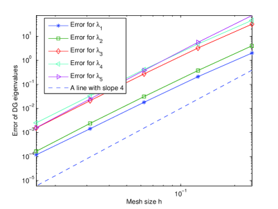
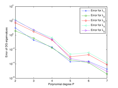
Figure 2: Error curves on the square using $P_{3}$ space with different mesh sizes (left) and different polynomial degrees (right).

Next we solve for the lowest 5 eigenvalues using $P_{3}$ polynomial space. The associated numerical eigenvalues and their error curves are shown in Table 5 and the left side of Figure 2, respectively. We see that the convergence rate of this case is around $O(h^{4})$ for all computed eigenvalues.

As the last numerical example in 2D, we apply the IPDG method to solve the eigenvalue problem on the square using different polynomial degrees with fixed mesh size. The right hand side of Figure 2 plots the error curves in the semi-log chart with fixed $h=1/8$ and polynomial degrees $p$ ranging from 2 to 7. It can be seen that the errors of the computed DG eigenvalues have a linear trend with respect to the local polynomial degrees in the semi-log scale, which indicates exponential rate of convergence. Numerically, it is $exp(-rp)$ with $r=2.5\sim 3$.

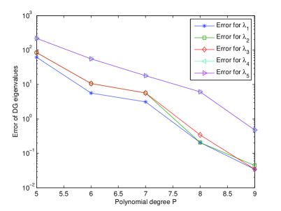
Figure 3: Error curves on the cube using different polynomial degrees with fixed mesh.

Finally, we show a numerical example on the three dimensional cube $[-1,1]^{3}$ with polynomial degrees $p$ ranging from 5 to 9. We divide the cube into six uniform tetrahedra and set $\eta_{1}=15.6$, $\eta_{2}=1.35$. The computed lowest five DG eigenvalues are listed in Table 6 and the associated error curves are plotted in Figure 3. Numerically, the convergence rates of the lowest five DG eigenvalues are $exp(-rp)$ with $r=0.10\sim 0.15$.

Acknowledgment. This work was supported in part by the National Natural Science Foundation of China Grants: 11871092, 12001130, 12131005, and NSAF 1930402, China Postdoctoral Science Foundation no. 2020M680316, and Science and Technology Foundation of Guizhou Province no. ZK[2021]012.

We thank Baijun Zhang in CSRC for his extensive discussions on this topic.

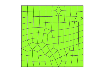
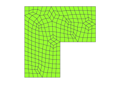
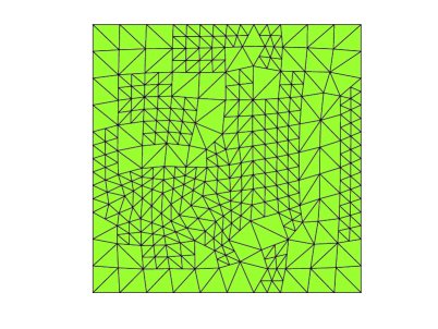
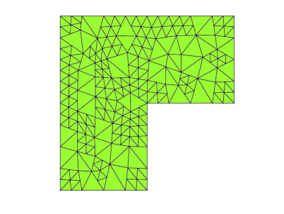
Figure 1: The quadrilateral meshes on the square (left top, 1428 DOFs) and on the L-shape domain(right top, 3024 DOFs); the triangular meshes with hanging nodes on the square (left bottom, 7176 DOFs, $\lambda_{1,h}\sim\lambda_{5,h}$: 7.0E+02, 7.07E+02, 2.3E+03, 4.2E+03, 5.0E+03) and on the L-shape domain(right bottom, 3816 DOFs, $\lambda_{1,h}\sim\lambda_{5,h}$: 33, 98, 3.8E+02, 4.0E+02, 6.8E+02)

Table 1: Numerical eigenvalues on the square using quadrilateral meshes

$h$	1/10	1/20	1/40	1/80	1/160
$\lambda_{1,h}$	762.9	726.7	713.4	709.4	708.3
$\lambda_{2,h}$	776.8	730.7	714.5	709.7	708.4
$\lambda_{3,h}$	2705.9	2478.4	2387.6	2360.1	2352.6
$\lambda_{4,h}$	3060.8	4425.8	4306.8	4269.7	4259.5
$\lambda_{5,h}$	4713.8	5221	5081	5039.3	5027.9
$|\lambda_{1,h}-\lambda_{1}|/\lambda_{1}$	0.0776	0.0265	0.0077	0.0020	0.0005
Rate				1.9264	2.1222
$|\lambda_{2,h}-\lambda_{2}|/\lambda_{2}$	0.0972	0.0321	0.0092	0.0024	0.0006
Rate				1.9175	2.0134
$|\lambda_{3,h}-\lambda_{3}|/\lambda_{3}$	0.1515	0.0546	0.0160	0.0043	0.0011
Rate				1.8949	1.9520
$|\lambda_{4,h}-\lambda_{4}|/\lambda_{4}$	0.2808	0.0399	0.0120	0.0033	0.0009
Rate				1.8765	1.9135
$|\lambda_{5,h}-\lambda_{5}|/\lambda_{5}$	0.0617	0.0392	0.0113	0.0030	0.0008
Rate				1.8969	1.9698

Table 2: Numerical eigenvalues on the L-shape using quadrilateral meshes

$h$	1/8	1/16	1/32	1/64	1/128
$\lambda_{1,h}$	35.3209	34.0426	33.6188	33.4995	33.4685
$\lambda_{2,h}$	58.0695	100.9415	99.1287	98.6054	98.4652
$\lambda_{3,h}$	72.6584	392.0341	384.0611	381.7741	381.1653
$\lambda_{4,h}$	106.2517	412.9257	402.516	399.245	398.2771
$\lambda_{5,h}$	440.7255	501.4575	688.5538	683.8663	682.5761
$|\lambda_{1,h}-\lambda_{1}|/\lambda_{1}$	0.0557	0.0175	0.0048	0.0013	0.0003
Rate				1.9386	1.9329
$|\lambda_{2,h}-\lambda_{2}|/\lambda_{2}$	0.4098	0.0256	0.0072	0.0019	0.0005
Rate				1.9135	1.9475
$|\lambda_{3,h}-\lambda_{3}|/\lambda_{3}$	0.8092	0.0291	0.0082	0.0021	0.0006
Rate				1.9231	1.9635
$|\lambda_{4,h}-\lambda_{4}|/\lambda_{4}$	0.7327	0.0377	0.0116	0.0033	0.0009
Rate				1.7890	1.8716
$|\lambda_{5,h}-\lambda_{5}|/\lambda_{5}$	0.3538	0.2648	0.0094	0.0026	0.0007
Rate				1.8817	1.9369

Table 3: Numerical eigenvalues on the square using uniform triangular meshes

$h$	1/8	1/16	1/32	1/64	1/128
$\lambda_{1,h}$	697.66	707.89	708.32	708.11	708.01
$\lambda_{2,h}$	703.97	709.47	708.67	708.19	708.03
$\lambda_{3,h}$	2294.94	2354.17	2353.56	2351.21	2350.34
$\lambda_{4,h}$	4112.82	4251.31	4259.09	4257.22	4256.24
$\lambda_{5,h}$	4912.41	5027.41	5028.64	5025.61	5024.45
$|\lambda_{1,h}-\lambda_{1}|/\lambda_{1}$	1.46e-02	1.12e-04	4.92e-04	1.95e-04	5.79e-05
Rate				1.3344	1.7510
$|\lambda_{2,h}-\lambda_{2}|/\lambda_{2}$	5.66e-03	2.12e-03	9.84e-04	3.04e-04	8.33e-05
Rate				1.6968	1.8655
$|\lambda_{3,h}-\lambda_{3}|/\lambda_{3}$	2.34e-02	1.78e-03	1.52e-03	5.22e-04	1.49e-04
Rate				1.5412	1.8097
$|\lambda_{4,h}-\lambda_{4}|/\lambda_{4}$	3.36e-02	1.06e-03	7.70e-04	3.29e-04	1.00e-04
Rate				1.2244	1.7186
$|\lambda_{5,h}-\lambda_{5}|/\lambda_{5}$	2.22e-02	6.80e-04	9.25e-04	3.21e-04	9.14e-05
Rate				1.5257	1.8141

Table 4: Numerical eigenvalues on the L-shape using uniform triangular meshes

$h$	1/8	1/16	1/32	1/64	1/128
$\lambda_{1,h}$	33.4608	33.4824	33.4664	33.4603	33.4589
$\lambda_{2,h}$	98.5124	98.5541	98.4667	98.4312	98.4204
$\lambda_{3,h}$	381.4047	381.6117	381.19	381.0231	380.9735
$\lambda_{4,h}$	396.4531	398.4319	398.177	397.9822	397.9045
$\lambda_{5,h}$	677.3528	682.6124	682.4738	682.2339	682.1436
$|\lambda_{1,h}-\lambda_{1}|/\lambda_{1}$	9.86e-05	7.44e-04	2.66e-04	8.37e-05	4.18e-05
Rate				1.6684	1.0000
$|\lambda_{2,h}-\lambda_{2}|/\lambda_{2}$	9.72e-04	1.40e-03	5.08e-04	1.47e-04	3.76e-05
Rate				1.7859	1.9705
$|\lambda_{3,h}-\lambda_{3}|/\lambda_{3}$	1.18e-03	1.72e-03	6.16e-04	1.78e-04	4.78e-05
Rate				1.7915	1.8973
$|\lambda_{4,h}-\lambda_{4}|/\lambda_{4}$	3.67e-03	1.30e-03	6.64e-04	1.73e-04	2.26e-05
Rate				1.9443	2.9323
$|\lambda_{5,h}-\lambda_{5}|/\lambda_{5}$	6.99e-03	7.22e-04	5.19e-04	1.67e-04	3.48e-05
Rate				1.6343	2.2661

Table 5: Numerical eigenvalues on the square by different polynomial degrees $p$: uniform triangular mesh $h=1/8$

$p$	2	3	4	5	6	7
$\lambda_{1,h}$	697.664507	708.181644	707.993329	707.971329	707.971765	707.971509
$\lambda_{2,h}$	703.966943	708.349258	707.989007	707.971929	707.971702	707.971551
$\lambda_{3,h}$	2294.939257	2353.247385	2350.206945	2349.986846	2349.987798	2349.985790
$\lambda_{4,h}$	4112.822158	4260.588288	4256.264643	4255.816486	4255.817946	4255.814058
$\lambda_{5,h}$	4912.406669	5029.614780	5024.259053	5023.992937	5023.992162	5023.992341

Table 6: Numerical eigenvalues on the cube by different polynomial degrees $p$: 6 uniform tetrahedra

$p$	5	6	7	8	9
$\lambda_{1,h}$	168.4810	112.2701	109.7608	106.8450	106.6736
$\lambda_{2,h}$	191.1329	117.3074	112.3088	106.8450	106.6834
$\lambda_{3,h}$	191.1329	117.3074	112.3088	106.9811	106.6737
$\lambda_{4,h}$	466.1273	302.4162	264.9300	253.0533	247.4130
$\lambda_{5,h}$	466.1273	302.4162	264.9300	253.0533	247.4129

Appendix A

We introduce the following function (with the Legendre polynomial $L_{i}(\widehat{x})$ of degree $i$)

$$\widehat{\phi}_{i}(\widehat{x})=\left\{\begin{tabular}[]{ll}$\frac{1-\widehat{x}}{2}$,&$i=0$,\\ $\frac{1+\widehat{x}}{2}$,&$i=1$,\\ $\frac{L_{i}(\widehat{x})-L_{i-2}(\widehat{x})}{\sqrt{2(2i-1)}}$,&$i\geq 2$.\\ \end{tabular}\right.$$ (5.4)

The basis functions of ${\bf H}(\mathrm{curl})$-conforming rectangular element in $Q^{p-1,p}([-1,1]^{2})\times Q^{p,p-1}([-1,1]^{2})$ is as follows.

A.

Cell-based basis functions:

I.

$\bm{\Phi}^{-}_{i,j}:=\nabla\widehat{\phi}_{i}(\widehat{x}_{1})\widehat{\phi}_{j}(\widehat{x}_{2})-\widehat{\phi}_{i}(\widehat{x}_{1})\nabla\widehat{\phi}_{j}(\widehat{x}_{2})$ for $2\leq i,j\leq p$.  ($(p-1)^{2}$ in total)

II.

$\bm{\Phi}^{+}_{i,j}:=\nabla\widehat{\phi}_{i}(\widehat{x}_{1})\widehat{\phi}_{j}(\widehat{x}_{2})+\widehat{\phi}_{i}(\widehat{x}_{1})\nabla\widehat{\phi}_{j}(\widehat{x}_{2})$ for $2\leq i,j\leq p$.  ($(p-1)^{2}$ in total)

III.

$\bm{\Phi}_{1,j}:=\widehat{\phi}_{j}(\widehat{x}_{2})\bm{e}_{1}$ and $\bm{\Phi}_{i,1}:=\widehat{\phi}_{i}(\widehat{x}_{1})\bm{e}_{2}$ for $2\leq i,j\leq p$.  ($2(p-1)$ in total)

B.

Edge-based basis functions

I.

$\bm{\Phi}^{+}_{i,j}:=\nabla\widehat{\phi}_{i}(\widehat{x}_{1})\widehat{\phi}_{j}(\widehat{x}_{2})+\widehat{\phi}_{i}(\widehat{x}_{1})\nabla\widehat{\phi}_{j}(\widehat{x}_{2})$ for $i=0,1$ and $2\leq j\leq p$. ($2(p-1)$ in total)

II.

$\bm{\Phi}^{+}_{i,j}:=\nabla\widehat{\phi}_{i}(\widehat{x}_{1})\widehat{\phi}_{j}(\widehat{x}_{2})+\widehat{\phi}_{i}(\widehat{x}_{1})\nabla\widehat{\phi}_{j}(\widehat{x}_{2})$ for $j=0,1$ and $2\leq i\leq p$. ($2(p-1)$ in total)

III.

$\bm{\Phi}_{-1,j}:=\widehat{\phi}_{j}(\widehat{x}_{2})\bm{e}_{1}$ and $\bm{\Phi}_{i,-1}:=\widehat{\phi}_{i}(\widehat{x}_{1})\bm{e}_{2}$ for $i,j=0,1$. ($4$ in total)

The above basis functions are orthogonal in the sense of $(\mathrm{curl}\cdot,\mathrm{curl}\cdot)$ and $<\gamma\cdot,\gamma\cdot>$ where $\gamma\bm{v}:=\widehat{\bm{v}}\cdot\tau$ is the tangential trace of $\bm{v}$. Let $\widehat{\bm{v}}\in\nabla(Q^{1,p}+Q^{p,1})$. Denote $\Pi(\widehat{\bm{v}}):=(\Pi_{1}(\widehat{\bm{v}}),\Pi_{2}(\widehat{\bm{v}}))^{T}$ with

$$\begin{aligned} \Pi_{1}(\widehat{\bm{v}})=\frac{1}{2}\int_{-1}^{1}\widehat{v}_{1}(\widehat{x}_{1},-1)d\widehat{x}_{1}\phi_{0}(\widehat{x}_{2})+\frac{1}{2}\int_{-1}^{1}\widehat{v}_{1}(\widehat{x}_{1},1))d\widehat{x}_{1}\phi_{1}(\widehat{x}_{2}),\\ \Pi_{2}(\widehat{\bm{v}})=\frac{1}{2}\int_{-1}^{1}\widehat{v}_{2}(-1,\widehat{x}_{2})d\widehat{x}_{2}\phi_{0}(\widehat{x}_{1})+\frac{1}{2}\int_{-1}^{1}\widehat{v}_{2}(1,\widehat{x}_{2}))d\widehat{x}_{2}\phi_{1}(\widehat{x}_{1}).\end{aligned}$$ (5.5)

Then $\widehat{\bm{v}}:=\bm{r}+\bm{t}+\Pi(\widehat{\bm{v}})$ with $\bm{r}=\Sigma_{i=0}^{1}\Sigma_{j=2}^{p}C^{+}_{i,j}\bm{\Phi}^{+}_{i,j}$ and $\bm{t}=\Sigma_{j=0}^{1}\Sigma_{i=2}^{p}C^{+}_{i,j}\bm{\Phi}^{+}_{i,j}$. One can verify that

$$\begin{aligned} \int_{[-1,1]^{2}}(r_{1}^{2}(1-\widehat{x}_{2}^{2})^{-1}+r_{2}^{2})d\bm{x}\lesssim\Sigma_{i=0}^{1}\Sigma_{j=2}^{p}(C^{+}_{i,j})^{2}((j^{2}-j)^{-1}+1),\\ \int_{[-1,1]^{2}}(t_{2}^{2}(1-\widehat{x}_{1}^{2})^{-1}+t_{1}^{2})d\bm{x}\lesssim\Sigma_{j=0}^{1}\Sigma_{i=2}^{p}(C^{+}_{i,j})^{2}((i^{2}-i)^{-1}+1).\end{aligned}$$ (5.6)

References

[1] D. N. Arnold, F. Brezzi, B. Cockburn, and L. D. Marini. Unified analysis of
discontinuous Galerkin methods for elliptic problems. SIAM J. Numer. Anal., 39 (2001),
1749-1779.
[2]M. Ainsworth and J. Coyle. Computation of Maxwell eigenvalues on curvilinear domains using hp-version Ndlec elements.
Numer. Math. Adv. Appl., 2003, 219-231.
[3]I. Babuska and J. Osborn. Eigenvalue Problems, in: P .G. Ciarlet, J. L. Lions, (Ed.), Finite Element Methods (Part 1),
Handbook of Numerical Analysis, vol.2, Elsevier Science Publishers,
North-Holand, 1991, 640-787.
[4]I. Babus̆ka and M. Suri. The hp version of the finite element method with quasiuniform meshes. M2AN, 21(1987) ,
199-238.
[5] G. A. Baker. Finite element methods for elliptic equations using nonconforming elements.
Math. Comp., 31(1977), 45-59.
[6] F. Ben Belgacem and C. Bernardi, Spectral element discretization of the Maxwell equations. Math. Comp., 68(1999), 1497-1520.
[7]A. Bespalov and N. Heuer. Optimal error estimation for H(curl)-conforming p-interpolation in two dimensions. SIAM J. Numer. Anal., 47(2009), 3977-3989
[8]D. Boffi. Fortin operator and discrete compactness for edge elements. Numer. Math., 87
(2000), 229-246.
[9]D. Boffi, M. Costabel, M. Dauge,
L. Demkowicz and R. Hiptmair. Discrete compactness for the p-version of discrete differential forms. SIAM J Numer. Anal., 49(2011), 135-158.
[10]D. Boffi, P. Guzman, and M. Neilan. Convergence of Lagrange finite elements for the Maxwell Eigenvalue problem in 2d. IMA J. Numer. Anal., (2022), to appear.
[11] A. Buffa, P. Ciarlet, and E. Jamelot. Solving electromagnetic eigenvalue problems in
polyhedral domains with nodal finite elements. Numer. Math., 113 (2009), 497-518.
[12] A. Buffa, P. Houston, and I. Perugia. Discontinuous Galerkin computation of the Maxwell
eigenvalues on simplicial meshes. J. Comput. Appl. Math., 204 (2007), 317-333.
[13]S. C. Brenner, F. Li , and L. Sung.
Nonconforming Maxwell eigensolvers. J. Sci. Comput., 40(2009), 51-85.
[14]S. C. Brenner. J. Sun, and L. Sung.
Hodge decomposition methods for a quad-curl problem on planar domains.
J. Sci. Comput., 73(2017), 495-513.
[15]F. Cakoni, D. Colton, P. Monk, and J. Sun.
The inverse electromagnetic scattering problem for anisotropic media.
Inverse Problems, 26(2010), 074004.
[16]A. Cangiani, Z. Dong,
E. H. Georgoulis, and P. Houston. hp-version discontinuous Galerkin methods on polygonal and polyhedral meshes.
Springer, Berlin, 2017.
[17]S. Cao, L. Chen and X. Huang. Error analysis of a decoupled finite element method for quad-curl
problems.
J Sci. Comput., 90(2022), https://doi.org/10.1007/s10915-021-01705-7.
[18]G. Chen, W. Qiu and L. Xu.
Analysis of an interior penalty DG method for the quad-curl
problem. IMA J Numer. Anal., 00(2020), 1-34.
[19]L. Chen. iFEM: An Integrated Finite Element Methods Package in MATLAB. Technical
report, University of California at Irvine, 2009.
[20] F. Chatelin. Spectral Approximations of Linear Operators. Academic Press, New York, 1983.
[21] P. Jr. Ciarlet, and G. Hechme. Computing electromagnetic eigenmodes with continuous
Galerkin approximations. Comput. Methods Appl. Mech. Engrg., 198 (2008),
358-365.
[22] B. Cockburn, G. E. Karniadakis, and C.-W. Shu. The development of discontinuous
Galerkin methods. in Discontinuous Galerkin methods (Newport, RI, 1999), vol. 11 of Lect.
Notes Comput. Sci. Eng., Springer, Berlin, 2000, 3-50.
[23] L. Demkowicz. Polynomial exact sequences and projection-based interpolation
with applications to Maxwell equations, in Mixed Finite Elements, Compatibility
Conditions, and Applications, D. Boffi and L. Gastaldi, eds., vol. 1939 of Lecture
Notes in Mathematics, Springer, Berlin, 2008, 101-158.
[24]Z. Dong. Discontinuous galerkin methods for the biharmonic problem on polygonal and polyhedral meshes.
Int. J. Numer. Anal. Mod., (2018)16, 825-846.
[25]X. Feng and O. A. Karakashian. Two-level non-overlapping Schwarz preconditioners
for a discontinuous Galerkin approximation of the biharmonic equation. J. Sci. Comput.,
22/23 (2005), 289-314.
[26] E. H. Georgoulis and P. Houston. Discontinuous Galerkin methods for the biharmonic
problem. IMA J. Numer. Anal., 29(2009), 573-594.
[27] E. H. Georgoulis, P. Houston, and J. Virtanen. An a posteriori error indicator for
discontinuous Galerkin approximations of fourth-order elliptic problems. IMA J. Numer.
Anal., 31 (2011), 281-298.
[28]E. Herbert and W. Christian. hp analysis of a hybrid DG method for Stokes flow. IMA Journal of Numerical Analysis, 2(2013), 687-721.
[29]K. Hu, Q. Zhang, and Z. Zhang. Simple curl-curl-conforming finite
elements in two dimensions. SIAM J
Sci. Comput., 42(2020), A3859-A3877.
[30]K. Hu, Q. Zhang, and Z. Zhang.
A family of finite element Stokes complexes in three dimensions. SIAM J Sci. Comput., (2022), https://doi.org/10.1137/20M1358700.
[31] R. Hiptmair. Finite elements in computational electromagnetism. Acta Numer., 11 (2002),
237-339.
[32]Q. Hong, J. Hun, S. Shu, and J. Xu. A discontinuous galerkin method for the
fourth-order curl problem. J. Comp. Math., 30(2012), 565-578.
[33]P. Houston, C. schwab, and E. süli.
Discontinuous hp-finite element methods for
advection-diffusion-reaction problems.
SIAM J. Numer. Anal., 39(2002), 2133-2163.
[34]P. Houston, I. Perugia, A. Schneebeli and D. Schötzau. Interior penalty method for the indefinite time-harmonic Maxwell equations. Numer. Math., 100(2005), 485-518.
[35]O. Karakashian and C. Collins. Two-level additive Schwarz methods for discontinuous
Galerkin approximations of the biharmonic equation. J. Sci. Comput., 74 (2018), 573-604.
[36]F. Kikuchi. Weak formulations for finite element analysis of an electromagnetic eigenvalue
problem. Scientific Papers of the College of Arts and Sciences, University of Tokyo, 38
(1988), 43-67.
[37]P. Monk, Finite Element Methods for Maxwell’s Equations. Oxford University Press, Oxford,
UK, 2003.
[38]P. Monk and J. Sun. Finite Element Methods for Maxwell’s tranmission eigenvalues. SIAM. J. Sci. Comput., 34(2012), B247-B264.
[39]P. Monk.
On the p- and hp-extension of Nedelec’s
curl-conforming elements. J. Comp. Appl. Math., 53(1994), 117-137.
[40] I. Mozolevski and E. Süli. A priori error analysis for the hp-version of the discontinuous Galerkin finite element method for the biharmonic equation, Comput. Methods Appl.
Math., 3 (2003), 596-607.
[41] I. Mozolevski, E. Süli, and P. R. Bösing. hp-version a priori error analysis of interior
penalty discontinuous Galerkin finite element approximations to the biharmonic equation.
J. Sci. Comput., 30 (2007), 465-491.
[42] J. C. Ndlec. Mixed finite elements in . Numer. Math., 35(1980), 315-341.
[43]J. Pan and H. Li, A penalized weak Galerkin spectral element method for second order elliptic equations. J. Comput. Appl. Math., 386(2021), 113228.
[44] D. Di Pietro and A. Ern. Mathematical aspects of discontinuous Galerkin methods,
vol. 69 of Mathématiques Applications (Berlin) [Mathematics Applications], Springer,
Heidelberg, 2012.
[45] S. Prudhomme, F. Pascal, J.T. Oden, and A. Romkes. Review of a priori error estimation
for discontinuous Galerkin methods, Tech. Report 2000-27, TICAM, University of Texas at
Austin, 2000.
[46] C. J. Reddy, M. D. Deshpande, C. R. Cockrell, and F. B. Beck. Finite Element Method for Eigenvalue Problems in Electromagnetics. Nasa Sti/recon Technical Report N, 95(1995).
[47]A. D. Russo and A. Alonso. Finite element approximation of Maxwell eigenproblems on curved Lipschitz polyhedral domains.
Appl. Numer. Math., 59(2009), 1796-1822.
[48]J. Sun. A mixed FEM for the quad-curl eigenvalue problem.
Numer. Math., 132(2016), 185-200
[49] J. Sun, Q. Zhang, and Z. Zhang. A curl-conforming weak Galerkin method for the quad-curl problem. BIT Numerical Mathematics, 59: 1093-1114, 2019.
[50]Z. Sun, J. Cui, F. Gao, and C. Wang. Multigrid methods for a quad-curl problem based on interior penalty method. Computers & Mathematics with Applications, 76(9): 2192-2211, 2018.
[51]E. Süli and I. Mozolevski. hp-version interior penalty DGFEMs for the biharmonic
equation. Comput. Methods Appl. Mech. Engrg., 196 (2007), 1851-1863
[52]L. Wang, W. Shan, H. Li, and Z. Zhang. -conforming quadrilateral spectral element method for quad-curl problems. Math. Mod. Meth. Appl. Sci., 31(2021), 1951-1986.
[53]Q. Zhang, L. Wang, and Z. Zhang.
An -conforming finite element in 2 dimensions and applications to the quad-curl problem. SIAM J. Sci. Comput., 41(2019), A1527-A1547.
[54] B. Zheng, B. Hu, and Q. Xu. A nonconforming element method for fourth order curl equations in . Math. Comput., 276(2011), 1871-1886.