Chemical enrichment in the cool core of the Centaurus cluster of galaxies

Abstract

Here we present results from over 500 kiloseconds Chandra and XMM-Newton observations of the cool core of the Centaurus cluster. We investigate the spatial distributions of the O, Mg, Si, S, Ar, Ca, Cr, Mn, Fe, and Ni abundances in the intracluster medium with CCD detectors, and those of N, O, Ne, Mg, Fe, and Ni with the Reflection Grating Spectrometer (RGS). The abundances of most of the elements show a sharp drop within the central 18 arcsec, although different detectors and atomic codes give significantly different values. The abundance ratios of the above elements, including Ne/Fe with RGS, show relatively flat radial distributions. In the innermost regions with the dominant Fe-L lines, the measurements of the absolute abundances are challenging. For example, AtomDB and SPEXACT give Fe $=$ 0.5 and 1.4 solar, respectively, for the spectra from the innermost region. These results suggest some systematic uncertainties in the atomic data and response matrices at least partly cause the abundance drop rather than the metal depletion into the cold dust. Except for super-solar N/Fe and Ni/Fe, sub-solar Ne/Fe, and Mg/Fe, the abundance pattern agrees with the solar composition. The entire pattern is challenging to reproduce with the latest supernova nucleosynthesis models. Observed super-solar N/O and comparable Mg abundance to stellar metallicity profiles imply the mass-loss winds dominate the intracluster medium in the brightest cluster galaxy. The solar Cr/Fe and Mn/Fe ratios indicate a significant contribution of near- and sub-Chandrasekhar mass explosions of Type Ia supernovae.

1 INTRODUCTION

Elemental abundances in stars and gas in the Universe provide stringent constraints on the formation and evolutionary history of galaxies. Excluding primordial elements in the Universe like H, He, Li, and Be, other heavy chemical elements were synthesised in stars and expelled into interstellar space by supernovae (SNe). Light $\alpha$-elements (O, Ne, Mg) mainly originate from core-collapse SNe (CCSNe), and Fe-peak ones (Cr, Mn, Fe, Ni) are, on the other hand, produced by thermonuclear explosions in Type Ia SNe (SNeIa). The intermediate-mass elements (IMEs), i.e. Si, S, Ar, and Ca, are synthesised by both SNeIa and CCSNe (e.g., Nomoto et al., 2013, and references therein). Unlike these elements, N is mainly synthesised in low- or intermediate-mass stars and expelled into the interstellar medium (ISM) through stellar mass loss (e.g., Nomoto et al., 2013).

The intracluster medium (ICM), hot X-ray emitting plasma pervading the galaxy clusters, retains a dominant fraction of heavy elements (e.g., N, O, Ne, Mg, Si, S, Ar, Ca, Cr, Mn, Fe, and Ni) synthesised by stars and SN explosions in member galaxies. The abundance of these elements can be well constrained from the intensity of their K-shell emission lines within the X-ray band (e.g., Mernier et al., 2018a, for a recent review). Therefore, X-ray spectroscopy of the ICM is one of the most reliable ways to investigate the chemical enrichment history in clusters (e.g., de Plaa et al., 2007; Sato et al., 2007; Mernier et al., 2018b). In the last few decades, spatially resolved spectra of the ICM observed with modern X-ray observatories like Chandra, XMM-Newton and Suzaku have allowed us to study the spatial distribution of metals in the ICM. Outside the core regions, flat and azimuthally uniform Fe distributions towards the outskirts have been reported (e.g., Matsushita, 2011; Matsushita et al., 2013a; Werner et al., 2013; Simionescu et al., 2015; Urban et al., 2017). This remarkably extended Fe distribution requires the early enrichment of the ICM before the cluster formation, i.e. ten billion years ago, also supported by cosmological simulations (e.g., Biffi et al., 2018).

X-ray luminous clusters showing a strong surface brightness peak towards the centre, i.e. cool-core clusters, are ideal targets to study ongoing enrichment process by the brightest cluster galaxies (BCGs). Most of them are classified as elliptical, and located in the X-ray peak of the cool cores. Observational studies of the metal abundances in cool cores provide a powerful probe for where and when metals were dispersed into the ICM. A central Fe abundance excess within the ICM was first reported in the Centaurus cluster by ROSAT and ASCA (Allen & Fabian, 1994; Fukazawa et al., 1994). Many other cool-core clusters exhibit similar trends for metal abundances (e.g., De Grandi & Molendi, 2001; Million et al., 2011; Mernier et al., 2017). To produce the central Fe abundance peaks, Böhringer et al. (2004) proposed enrichment by SNeIa over a relatively long time ($>5$ Gyr). In addition, metal enrichment by CCSNe when the cluster galaxies were still actively star-forming has been discussed based on central peaks of $\alpha$-elements (e.g., de Plaa et al., 2006; Simionescu et al., 2009; Mernier et al., 2017; Erdim et al., 2021). Recent observation in the Perseus cluster core by Hitomi provided compelling results that the O/Fe, Ne/Fe, Mg/Fe, Si/Fe, S/Fe, Ar/Fe, Ca/Fe, Cr/Fe, Mn/Fe, and Ni/Fe abundance ratios in the ICM are fully consistent with those in the solar, and therefore the Milky Way (Hitomi Collaboration et al., 2017; Simionescu et al., 2019). This solar chemical composition in the Perseus core requires not only CCSN but also near- and sub-Chandrasekhar mass ($M_{\textrm{Ch}}$) SNIa contribution to the enrichment of the ICM. Although the abundance ratio pattern could not be reproduced sufficiently by the latest SN nucleosynthesis models, the study of the Perseus core provided an important clue to chemical enrichment in the cluster centre and possibly BCG.

Within a central few-kiloparsec, the situation is more puzzling and fascinating in the innermost core. Since the first discovery in A2199 (Johnstone et al., 2002), central abundance drops are reported especially for Fe in some cool-core clusters wherein the enhanced enrichment is expected from the central BCG (e.g., Churazov et al., 2003; Panagoulia et al., 2015; Liu et al., 2019). The central abundance drop in the Centaurus cluster was first discovered by Sanders & Fabian (2002) with a remarkable depletion from $\sim$ 2 to $\sim$ 0.5 solar towards the centre. With optical and infrared observations, cold dust filaments are detected in BCGs (e.g., Crawford et al., 2005; Mittal et al., 2011, for the Centaurus cluster), and Panagoulia et al. (2015) proposed that these abundance drops would be caused by depletion of metals into the cool dust grains in the BCG. Lakhchaura et al. (2019) reported that the abundance of the ‘non-reactive’ element Ar shows a relatively slight central drop, while Si and S show a remarkable abundance drop as Fe. The abundance drops may originate from the feedback of active galactic nuclei which would dissipate a fraction of central metal-rich gas towards the outer radius (e.g., Sanders et al., 2016; Liu et al., 2019).

The Centaurus cluster, also known as A3526, is a well-known cool-core cluster, within which NGC 4696 is residing as the BCG. Because being a nearby and X-ray luminous galaxy cluster, the Centaurus cluster is one of the most compelling examples as well as the Perseus cluster for studies of the metal abundance in the ICM. It has been reported that the abundance in a few-arcmin core of the Centaurus cluster shows super-solar ($\sim$ 1.5–2 solar) value for IMEs and Fe by X-ray missions like Chandra, XMM-Newton, and Suzaku (e.g., Matsushita et al., 2007; Takahashi et al., 2009; Sakuma et al., 2011; Sanders et al., 2016). The Fe abundance in other cluster cores, on the other hand, is typically sub-solar ($\sim$ 0.8 solar), which is close to those of groups and early-type galaxies (e.g., Konami et al., 2014; Mernier et al., 2018c). Then, the Centaurus cluster core do be the specific but ideal target for a comprehensive study of SNIa contribution to the enrichment due to the high Fe abundance.

In this paper, we analyse the deepest CCD data with Chandra and XMM-Newton to date of the cool core of the Centaurus cluster and NGC 4696. We study the spatial distributions of metal abundances of O, Mg, IMEs, and Fe-peak elements, including Cr, Mn, and Ni, to constrain the metal enrichment history by the BCG. In addition, we analyse grating data onboard XMM-Newton to study the spatial distribution of Ne and N. Due to its non-chemical reactivity, radial distribution of the Ne abundance would be crucial to restrict the mechanism of abundance drops at the cluster centre. We also make a comparison between the latest versions of two different atomic codes, the atomic data base (AtomDB, Foster et al. 2012) and the spex Atomic Code and Tables (SPEXACT, Kaastra et al. 1996), which have been updated in response to Hitomi (Hitomi Collaboration et al., 2018b). This paper is organized as follows. In Section 2, we describe details of our Chandra and XMM-Newton observations and data reduction. In Section 3, we present our spectral analysis. We discuss the results in Section 4 and present our conclusions in Section 5. In this paper, we assume cosmological parameters as $H_{0}=70$ km s^-1 Mpc^-1, $\Omega_{m}=0.3$ and $\Omega_{\Lambda}=0.7$, for which 1 arcsec corresponds to $\sim$ 0.2 kpc at the redshift of 0.0114 for NGC 4696 (Struble & Rood, 1999). All abundances in this work are relative to the proto-solar values of Lodders et al. (2009). The errors are at 1$\sigma$ confidence level unless otherwise stated.

2 OBSERVATIONS AND DATA REDUCTION

We used the publicly archival observation data of the core region of the Centaurus cluster with the Chandra Advanced CCD Imaging Spectrometer (ACIS, Weisskopf et al. 2002), the European Photon Imaging Camera (EPIC, Turner et al. 2001; Strüder et al. 2001), and Reflecting Grating Spectrometer (RGS, den Herder et al. 2001) on-board XMM-Newton. Table 1 lists the observations used in this work.

Table 1: List of observations used in this work

Obs. ID	Instrument	Cleaned Exposure	Offseta	Date
		(ks)	(arcmin)
Chandra
504	ACIS-S	20.85	0.13	2000 May 22
505	ACIS-S	8.97	0.13	2000 Jun 08
4190	ACIS-S	30.52	3.79	2003 Apr 18
4191	ACIS-S	30.20	4.23	2003 Apr 18
4954	ACIS-S	73.73	0.10	2004 Apr 01
4955	ACIS-S	36.33	0.10	2004 Apr 02
5310	ACIS-S	40.60	0.10	2004 Apr 04
16223	ACIS-S	144.72	0.10	2014 May 26
16224	ACIS-S	29.40	0.10	2014 Apr 09
16225	ACIS-S	28.32	0.10	2014 Apr 26
16534	ACIS-S	47.17	0.10	2014 Jun 05
16607	ACIS-S	39.92	0.10	2014 Apr 12
16608	ACIS-S	23.09	0.10	2014 Apr 07
16609	ACIS-S	71.97	0.10	2014 May 04
16610	ACIS-S	16.43	0.10	2014 Apr 27
XMM-Newton
0046340101	MOS1	43.26	0.002	2002 Jan 03
	MOS2	43.55
	pn	30.46
	RGS1	44.83
	RGS2	43.51
0406200101	MOS1	100.91	0.11	2007 Aug 22
	MOS2	103.69
	pn	71.88
	RGS1	101.58
	RGS2	101.58
0823580101	MOS1	102.26	10.7	2018 Jul 03
	MOS2	104.39
	pn	104.39
0823580201	MOS1	100.77	11.6	2018 Aug 09
	MOS2	102.79
	pn	76.06
0823580501	MOS1	96.85	10.3	2018 Jul 20
	MOS2	98.37
	pn	72.65
0823580601	MOS1	99.88	11.3	2018 Jul 30
	MOS2	99.78
	pn	74.25

• The angular distance from NGC 4696 to the target coordinates of each observation.

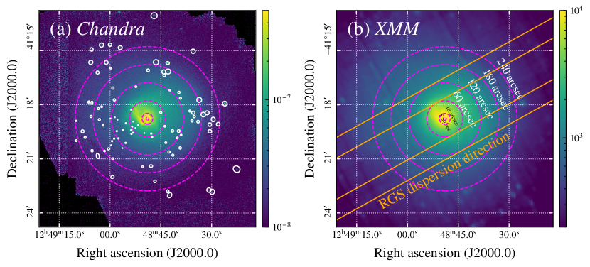
Figure 1: Images of the Centaurus cluster core in the $0.5$–$7.0$ keV band. (a) Vignetting corrected image with the Chandra ACIS-S, where the colour bar indicates photon flux in cm^-2 s^-1. The magenta dashed annuli represent 5, 18, 60, 120, 180, and 240 arcsec spectrum extraction regions. The white ellipses show the detected point sources (see § 2.1 for details). (b) A mosaiced count image with the XMM-Newton EPIC MOS and pn. The extraction region for RGS spectra (60–120 arcsec width on both sides, for instance) is shown with the orange lines, where the cross-dispersion width of RGS is between 60 and 120 arcsec lines.

2.1 Chandra

We used Chandra Interactive Analysis of Observations (ciao) version 4.12 (Fruscione et al., 2006) and calibration database (caldb) version 4.8.4.1 for the following data reduction. We reprocessed the data with chandra_repro tool keeping the standard procedure by Chandra team, and remove strong background flares using deflare script in the ciao package. The cleaned ACIS data have a total exposure of 640 ks after the procedures stated above. We also searched for faint point sources using the wavdetect algorithm in the energy range of 0.5–7.0 keV (encircled counts fraction $=0.9$, threshold significance $=10^{-6}$), excluding sources detected at the cluster centre and the surrounding ICM (e.g., plume-like structure, Sanders et al. 2016). We extracted ACIS spectra from the annular regions shown in Fig. 1(a) and generated redistribution matrix files (RMFs) and ancillary response files (ARFs) for each ObsID. The outermost radius of our extracting regions (240 arcsec) is about three times the effective radius ($R_{\textrm{e}}$) of NGC 4696 ($\sim$ 85 arcsec, Carollo et al. 1993), indicating that most of stars in NGC 4696 are within our extraction regions. In addition, this aperture is close to a radius at which the ICM temperature starts to decline towards the centre (Sanders et al., 2016). The spectra and response files taken in the same observation years are coadded to improve the photon statistics. Background spectra are extracted from all field of view of ACIS-S3 chip out of 3 arcmin core centred on the cluster centre.

2.2 XMM-Newton

2.2.1 EPIC

The reduction procedure for the data sets of XMM-Newton was performed using the XMM-Newton Science Analysis System (sas) version 18.0.0. We reprocessed and filtered all the EPIC data using emchain and epchain for the MOS and pn, respectively. The excluding sources are taken from the Chandra ACIS detection (Fig. 1(a)) at the same position and radius. All reprocess procedures are in accordance with the standard reduction criteria by sas. After the reprocess, the total exposure times are 550 ks (MOS), and 380 ks (pn). For each observation, we extracted EPIC spectra from the same annular regions as Chandra (Fig. 1(b)) and generated RMFs and ARFs for each ObsID, but did not merge them because the aim points of each observation are significantly shifted. We fit the spectra of MOS1 and MOS2 jointly with the same spectral parameters. The background spectra were extracted from the annular region with 7.5–11.7 arcmin.

2.2.2 RGS

The RGS spectra provide us spatial information of extended emission over 5 arcmin width along the cross-dispersion direction when the X-ray peak of the target locates near the pointing position (e.g., Chen et al., 2018; Zhang et al., 2019). Thus, we used only two datasets in 2002 and 2007 which have quite smaller offsets than the others (see Table 1). The RGS data were processed with rgsproc. After filtering flared events as well as the EPIC data, the remaining total exposure time is 140 ks. As done by Chen et al. (2018), we extracted first- and second-order RGS spectra centred on the emission peak along the dispersion direction instead of using the xpsfincl which is generally used. For each annular region within 120 arcsec for the CCD spectra, we filtered events by the cross-dispersion direction and extracted spectra over two wide regions on both sides. For instance, the two wide regions for 60–120 arcsec are plotted in Fig. 1(b). The first- and second-order spectra are jointly fitted, where the RGS1 and RGS2 spectra of each order are combined.

3 ANALYSIS & RESULTS

3.1 Spectral Fitting

3.1.1 CCD spectra

Here we analyse X-ray spectra extracted from the annular regions given in Fig. 1 using xspec package version 12.10.1f (Arnaud, 1996). We use the latest AtomDB version 3.0.9 to model a collisional ionization equilibrium (CIE) plasma. We model and fit the background spectra simultaneously with the source spectra, instead of subtracting them from the source data. The detector background model consists of a broken power-law with Gaussian lines for the instrumental fluorescence lines like Al-K, Si-K, and Cu-K (e.g., Leccardi & Molendi, 2008; Mernier et al., 2015). We also take the background celestial emissions into account with a power-law (1.4 photon index) for the cosmic X-ray background and two CIE plasma components with solar metallicity for the local hot bubble (LHB) and the Galactic thermal emission (e.g. Yoshino et al., 2009). These components except for the LHB are modified by the Galactic absorption and the temperature of the LHB is fixed at 0.1 keV. The derived temperature of the Galactic thermal emission is $0.94\pm 0.02$ keV, indicating that the Centaurus cluster is located at a high-temperature region of the Galactic emission (Yoshino et al., 2009; Nakashima et al., 2018). Because the ICM of the Centaurus cluster is extended over several degrees, the emission component from the ICM is also included in the spectral fitting model for the background region. In the following spectral analysis, we fit all spectra using the C-statistics (Cash, 1979), to estimate the model parameters and their error ranges without bias (Kaastra, 2017). The spectra are rebinned to have a minimum of 1 count per spectral bin. The stacked spectra of the central 240 arcsec region are shown in the upper panel of Fig. 2. Emission lines of O, Fe-L (+ Ne), Mg, Si, S, Ar, Ca, Fe and Ni (+ Fe) are clearly seen in the spectra. In addition, there are some hints of Cr and Mn lines in the pn spectrum.

Systematic uncertainties in the response matrices and atomic codes bias measurements of line and continuum temperatures. Therefore, we adopt bvvtapec model, which allows different temperatures for the line and continuum (e.g., Hitomi Collaboration et al., 2018a, for detailed discussion). The ICM spectra are modelled with a triple bvvtapec components to consider the multi-temperature structure in the cool core. We assume the three thermal components have the same metal abundances. The Galactic absorption is modelled using the phabs assuming the photoelectric absorption cross-sections taken from Verner et al. (1996). We let the absorption column density $N_{\textrm{H}}$ and elemental abundance of O, Ne, Mg, Si, S, Ar, Ca, Cr, Mn, Fe, and Ni vary freely. The abundances of elements lighter than O are fixed to solar. The other element abundances are tied to those of the nearest lower atomic number element, which is allowed to vary. For example, the F abundance is linked to that of O. The line and continuum temperatures for the middle- and coolest-temperature components cannot be well constrained independently and thus are assumed to be halved and quartered the hottest-temperature ones, respectively. We also let the volume emission measure (VEM) free to vary, given as $\int n_{e}n_{\textrm{H}}dV/(4\pi D^{2})$, where $n_{e}$ and $n_{\textrm{H}}$ is electron and proton density, $V$ and $D$ are the volume of the emission region and the distance to the emitting source, respectively. This model gives good fits to the spectra of the individual annular regions, yielding C-stat/dof $\sim 1$–$1.3$ as summarised in Table 2 and Fig. 2. Since the differences between line and continuum temperatures are small ($<0.3$ keV), we hereafter report the continuum temperature as representative. As shown in Fig. 3, the different CCD detectors give consistent VEM-weighted average temperatures (denoted $kT$) for each annular region. This profile shows a peak temperature of $\sim$ 3 keV and a clear drop towards the centre, which is consistent with a more extended profile by Sanders et al. (2016). Therefore, our extracting regions cover an important part of the cool core of the Centaurus cluster as noted in § 2.1.

Next, we re-fit the spectra within local energy bands around the K-shell emission lines of the individual elements in order to minimize biases due to the response uncertainty on the metal abundance measurements, i.e. we perform local or narrow-band fits (e.g., Lakhchaura et al., 2019; Simionescu et al., 2019). The ratios of each VEM are fixed to the value of global fit, leaving the abundance of a considered element to vary freely and tying all other parameters to the global fit values in Table 2. The boundaries of these local bands are 0.51–0.77 keV for O, 0.75–1.25 keV for Ne, 1.36–1.59 keV for Mg, 1.65–2.26 keV for Si, 2.37–4.44 keV for other intermediate-mass elements (IMEs), i.e. S, Ar, and Ca, 5.01–6.59 keV for Cr and Mn, 6.25–7.25 keV for Fe, and 7.24–8.02 keV for Ni. Here, to avoid contaminations from the strong instrumental Cu line, we use the two observations pointing towards the cluster centre for the local-fits around the Ni lines of the pn spectra. The representative spectrum and the best-fitting residuals around each prominent line are plotted in the lower panels of Fig. 2. The obtained elemental abundances with the local fits are shown in Table 3 and 4. In Fig. 4, we compare the derived abundances from the global and local fits. The abundance values and the residual structure around each K-shell emission line with two fit methods are globally similar except for the Cr abundances. The Ne abundances with two fit methods are globally consistent, except for the results with pn which offers a relatively lower spectral resolution than that of MOS. However, the Ne K-shell emission lines are blended in the Fe-L bump, and thus, our estimation of the Ne abundances from the CCD spectra would be suffered from some systematic uncertainties. The Mg-K shell lines are also blended in the Fe-L bump. The Mg abundances with pn and ACIS show a relatively large scatter, while those with MOS, possibly the most reliable instrument among the three, are consistent except for only one point. We suspect that these discrepancies are mainly caused by the moderate spectral resolution and/or sensitivity of the pn and ACIS instruments. The local fits around the Fe-K lines mostly give consistent results with those from the global fits. The exceptions are the three regions within 60  arcsec with Chandra and the innermost region with pn, where the local fits give even lower Fe abundances than the global fits. Hereafter, we use the results of the global fits for the Fe abundance, and those of the local fits for the other elements.

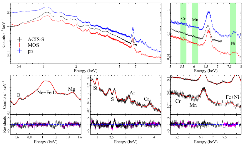
Figure 2: Upper: The stacked spectra of the central 240 arcsec region for each CCD camera, all of which are folded through the spectral response of each detector. The black, red, and blue data represent ACIS-S, MOS, and pn spectra, respectively. We also plot narrow band spectra in order to show the emission lines of Fe-peak elements. Lower: The representative spectra extracted from 18–60 arcsec annular region for MOS and best-fitting models enlarging on prominent K-shell emission lines. The black and magenta residuals represent the global and local fit results, respectively (see § 3.1.1 for detail). The pn spectrum is also plotted with diamonds for the Fe-peak elements. Emission lines for some elements are marked.

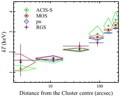
Figure 3: Radial profile of the VEM-weighted average temperature. The green-, red-, and blue-diamond plots are for results with Chandra ACIS-S, XMM-Newton MOS, pn, respectively. The magenta plots indicate the RGS results.

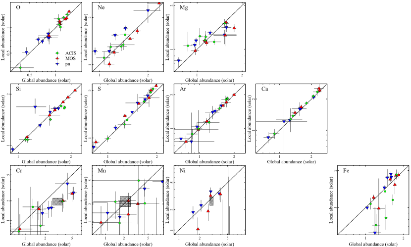
Figure 4: Comparisons of the element abundances in each annular region obtained from global fit with local one. The circle plots indicate the values with ACIS-S3, while the up- and down-triangle ones are for MOS and pn, respectively. The shaded squares for Fe-peak elements are the mean abundances of all CCDs measured in 18–120 arcsec region.

Table 2: Best-fitting spectral parameters for the ICM emission from the global fits.

Radial range	$N_{\textrm{H}}$a	$kT_{\textrm{hot}}$	$kT$b	VEM${}_{\textrm{hot}}$c	VEM${}_{\textrm{middle}}$	VEM${}_{\textrm{cool}}$	Fe	C-stat/dof
(arcsec)	(1020 cm-2)	(keV)	(keV)	(1010 cm-5)	(1010 cm-5)	(1010 cm-5)	(solar)
Chandra ACIS-S
$0$–$5$	$9.65$d	$2.51\pm 0.08$	$1.19\pm 0.14$	$0.5\pm 0.1$	$1.85\pm 0.06$	$1.29\pm 0.03$	$1.21\pm 0.09$	3233.5/2935
$5$–$18$	$11.9\pm 0.6$	$3.02\pm 0.09$	$1.59\pm 0.14$	$2.7\pm 0.3$	$10.0\pm 0.5$	$3.7\pm 0.1$	$1.44\pm 0.06$	3690.4/3435
$18$–$60$	$14.0\pm 0.2$	$3.05\pm 0.04$	$2.10\pm 0.09$	$31\pm 1$	$60\pm 1$	$0.88\pm 0.07$	$1.64\pm 0.02$	4476.1/3624
$60$–$120$	$13.2\pm 0.2$	$4.81\pm 0.12$	$2.9\pm 0.4$	$25\pm 5$	$94\pm 4$	$<0.02$	$1.76\pm 0.02$	4315.0/3636
$120$–$180$	$13.3\pm 0.2$	$5.47\pm 0.22$	$3.3\pm 0.4$	$24\pm 4$	$87\pm 4$	$<0.04$	$1.43\pm 0.02$	4246.0/3637
$180$–$240$	$14.8\pm 0.3$	$5.43\pm 0.09$	$3.6\pm 0.6$	$30\pm 6$	$59\pm 6$	$<0.35$	$1.09\pm 0.03$	4120.9/3637
XMM-Newton MOS
$0$–$5$	$8.7\pm 1.6$	$3.0\pm 0.3$	$1.5\pm 0.4$	$0.2\pm 0.1$	$0.8\pm 0.1$	$0.56\pm 0.08$	$1.27\pm 0.15$	33650.7/32951
$5$–$18$	$9.1\pm 0.5$	$3.05\pm 0.07$	$1.71\pm 0.12$	$2.7\pm 0.2$	$7.4\pm 0.3$	$2.46\pm 0.08$	$1.70\pm 0.05$	39746.3/38544
$18$–$60$	$10.3\pm 0.2$	$3.19\pm 0.04$	$2.14\pm 0.08$	$25.0\pm 0.8$	$44.7\pm 0.9$	$1.72\pm 0.06$	$1.83\pm 0.03$	48983.6/45484
$60$–$120$	$10.0\pm 0.2$	$4.10\pm 0.05$	$2.75\pm 0.12$	$39.8\pm 1.6$	$75.3\pm 1.7$	$1.0\pm 0.1$	$1.73\pm 0.02$	52423.1/49521
$120$–$180$	$9.5\pm 0.2$	$3.11\pm 0.03$	$3.10\pm 0.06$	$99.1\pm 0.9$	$0.7\pm 0.4$	$0.14\pm 0.04$	$1.57\pm 0.02$	53470.1/51021
$180$–$240$	$9.7\pm 0.2$	$3.35\pm 0.04$	$3.34\pm 0.17$	$93.1\pm 0.9$	$<0.32$	$0.19\pm 0.05$	$1.16\pm 0.02$	53906.0/51525
XMM-Newton pn
$0$–$5$	$9.2\pm 1.6$	$3.2\pm 0.3$	$1.5\pm 0.4$	$0.18\pm 0.07$	$0.87\pm 0.09$	$0.56\pm 0.09$	$1.19\pm 0.13$	17058.5/17149
$5$–$18$	$9.0\pm 0.5$	$3.03\pm 0.08$	$1.67\pm 0.14$	$2.6\pm 0.2$	$8.1\pm 0.4$	$2.6\pm 0.1$	$1.48\pm 0.06$	20386.6/20754
$18$–$60$	$10.4\pm 0.2$	$3.20\pm 0.04$	$2.11\pm 0.08$	$26.7\pm 1.0$	$51.3\pm 1.0$	$2.28\pm 0.07$	$1.58\pm 0.03$	25294.5/24836
$60$–$120$	$9.8\pm 0.1$	$4.17\pm 0.04$	$2.68\pm 0.08$	$35.2\pm 1.7$	$84.9\pm 0.4$	$1.44\pm 0.06$	$1.60\pm 0.01$	26942.3/24630
$120$–$180$	$9.2\pm 0.1$	$3.98\pm 0.02$	$2.95\pm 0.03$	$106.9\pm 0.1$	$1.5\pm 0.2$	$0.30\pm 0.03$	$1.41\pm 0.01$	26862.7/26803
$180$–$240$	$9.5\pm 0.1$	$3.18\pm 0.02$	$3.17\pm 0.02$	$103.4\pm 0.1$	$<0.20$	$0.30\pm 0.04$	$1.03\pm 0.01$	27476.0/27085
XMM-Newton RGS
$0$–$5$	$12.2$e	$3.02\pm 0.09$	$1.6\pm 0.8$	$<6.73$	$22\pm 5$	$3.4\pm 0.6$	$0.58\pm 0.10$	5303.1/5662
$5$–$18$	$12.2$	$1.70\pm 0.03$	$1.62\pm 0.12$	$51\pm 2$	$4.0\pm 0.2$	$1.0\pm 0.1$	$1.09\pm 0.10$	6799.2/6824
$18$–$60$	$12.2$	$3.55\pm 0.08$	$2.3\pm 0.2$	$54\pm 4$	$114\pm 6$	$3.4\pm 0.4$	$1.39\pm 0.11$	7685.8/7271
$60$–$120$	$12.2$	$2.52\pm 0.11$	$2.46\pm 0.17$	$114\pm 4$	$4.8\pm 0.8$	$9.4\pm 0.1$	$1.46\pm 0.10$	7585.3/7266

• The absorption cross sections are taken from Verner et al. (1996).

• The VEM-weighted average temperature.

• The volume emission measure (VEM) is given as $\int n_{e}n_{\textrm{H}}dV/(4\pi D^{2})$, where $V$ and $D$ are the volume of the emission region (cm³) and the distance to the emitting source (cm), respectively.

• We fix this parameter to the best-fitting value.

• Hydrogen column density towards the Centaurus cluster taken from http://www.swift.ac.uk/analysis/nhtot/.

Table 3: Abundances of N, O, Ne, Mg, Si, S, Ar, Ca, and Fe derived from the local fits (CCDs) and the global fits (RGS) with respect to the proto-solar values in Lodders et al. (2009).

Radial range	N	O	Ne	Mg	Si	S	Ar	Ca	Fe
(arcsec)	(solar)	(solar)	(solar)	(solar)	(solar)	(solar)	(solar)	(solar)	(solar)
Chandra ACIS-S (local)
$0$–$5$	–	$0.34\pm 0.08$	$1.34\pm 0.10$	$1.12\pm 0.05$	$1.09\pm 0.03$	$1.22\pm 0.07$	$1.13\pm 0.23$	$1.28\pm 0.35$	$0.71\pm 0.16$
$5$–$18$	–	$1.02\pm 0.11$	$2.73\pm 0.17$	$1.51\pm 0.11$	$1.70\pm 0.06$	$2.04\pm 0.07$	$1.81\pm 0.15$	$2.4\pm 0.2$	$0.8\pm 0.2$
$18$–$60$	–	$1.32\pm 0.05$	$1.31\pm 0.08$	$1.22\pm 0.04$	$1.65\pm 0.02$	$1.93\pm 0.03$	$1.86\pm 0.06$	$2.14\pm 0.08$	$1.15\pm 0.12$
$60$–$120$	–	$1.43\pm 0.09$	$1.55\pm 0.08$	$1.15\pm 0.18$	$1.68\pm 0.03$	$1.70\pm 0.03$	$1.51\pm 0.06$	$1.82\pm 0.07$	$1.85\pm 0.19$
$120$–$180$	–	$1.09\pm 0.10$	$1.30\pm 0.08$	$1.23\pm 0.17$	$1.42\pm 0.03$	$1.30\pm 0.04$	$1.00\pm 0.07$	$1.38\pm 0.08$	$1.35\pm 0.13$
$180$–$240$	–	$1.28\pm 0.17$	$1.11\pm 0.10$	$1.1\pm 0.3$	$1.08\pm 0.04$	$0.99\pm 0.05$	$0.89\pm 0.10$	$0.93\pm 0.10$	$1.07\pm 0.13$
XMM-Newton MOS (local)
$0$–$5$	–	$0.80\pm 0.17$	$2.5\pm 0.3$	$1.3\pm 0.2$	$1.54\pm 0.14$	$1.8\pm 0.2$	$0.9\pm 0.5$	$<0.60$	$1.0\pm 0.7$
$5$–$18$	–	$1.11\pm 0.09$	$2.87\pm 0.12$	$1.40\pm 0.09$	$2.08\pm 0.06$	$2.00\pm 0.09$	$1.81\pm 0.19$	$2.5\pm 0.3$	$1.5\pm 0.3$
$18$–$60$	–	$1.55\pm 0.06$	$1.64\pm 0.07$	$1.53\pm 0.04$	$2.03\pm 0.03$	$2.14\pm 0.04$	$2.17\pm 0.08$	$2.88\pm 0.10$	$1.83\pm 0.12$
$60$–$120$	–	$1.26\pm 0.06$	$1.01\pm 0.05$	$1.15\pm 0.04$	$1.81\pm 0.02$	$1.65\pm 0.03$	$1.72\pm 0.07$	$2.42\pm 0.08$	$1.82\pm 0.08$
$120$–$180$	–	$1.30\pm 0.07$	$1.46\pm 0.06$	$1.11\pm 0.05$	$1.59\pm 0.03$	$1.38\pm 0.04$	$1.34\pm 0.09$	$1.68\pm 0.08$	$1.69\pm 0.08$
$180$–$240$	–	$1.19\pm 0.09$	$1.19\pm 0.07$	$0.98\pm 0.06$	$1.14\pm 0.03$	$0.94\pm 0.04$	$0.97\pm 0.11$	$1.48\pm 0.10$	$1.21\pm 0.06$
XMM-Newton pn (local)
$0$–$5$	–	$0.76\pm 0.13$	$2.2\pm 0.4$	$1.26\pm 0.17$	$1.7\pm 0.2$	$1.7\pm 0.2$	$0.8\pm 0.6$	$1.2\pm 0.7$	$0.6\pm 0.4$
$5$–$18$	–	$0.77\pm 0.07$	$2.60\pm 0.12$	$1.41\pm 0.10$	$1.65\pm 0.06$	$1.85\pm 0.09$	$1.40\pm 0.19$	$1.6\pm 0.3$	$1.8\pm 0.3$
$18$–$60$	–	$0.85\pm 0.04$	$1.22\pm 0.07$	$1.30\pm 0.05$	$1.65\pm 0.03$	$1.75\pm 0.04$	$1.60\pm 0.08$	$2.09\pm 0.10$	$1.87\pm 0.10$
$60$–$120$	–	$0.69\pm 0.05$	$1.22\pm 0.07$	$1.15\pm 0.05$	$1.55\pm 0.03$	$1.46\pm 0.03$	$1.43\pm 0.07$	$1.61\pm 0.08$	$1.77\pm 0.06$
$120$–$180$	–	$0.72\pm 0.08$	$1.71\pm 0.07$	$1.07\pm 0.06$	$1.31\pm 0.04$	$1.16\pm 0.05$	$1.04\pm 0.10$	$1.25\pm 0.09$	$1.45\pm 0.06$
$180$–$240$	–	$0.51\pm 0.07$	$1.54\pm 0.11$	$0.84\pm 0.10$	$0.95\pm 0.03$	$0.88\pm 0.05$	$0.81\pm 0.12$	$0.85\pm 0.10$	$1.00\pm 0.04$
XMM-Newton RGS (global)
$0$–$5$	$0.8\pm 0.4$	$0.54\pm 0.09$	$0.42\pm 0.10$	$0.42\pm 0.09$	–	–	–	–	$0.58\pm 0.10$
$5$–$18$	$2.0\pm 0.5$	$0.93\pm 0.09$	$0.74\pm 0.10$	$0.82\pm 0.12$	–	–	–	–	$1.09\pm 0.10$
$18$–$60$	$2.3\pm 0.5$	$1.31\pm 0.11$	$0.99\pm 0.14$	$1.03\pm 0.12$	–	–	–	–	$1.39\pm 0.11$
$60$–$120$	$<0.47$	$1.40\pm 0.15$	$0.76\pm 0.15$	$0.62\pm 0.18$	–	–	–	–	$1.46\pm 0.10$

Table 4: Abundances of Fe-peak elements derived from the local fits (CCDs, except for Ni of ACIS) and global fits (Ni of ACIS and RGS) with respect to the proto-solar values in Lodders et al. (2009).

Radial range	Cr	Mn	Ni
(arcsec)	(solar)	(solar)	(solar)
Chandra ACIS-S
$0$–$5$	$<2.69$	$<6.43$	$3.5\pm 0.4$
$5$–$18$	$<1.52$	$<3.31$	$4\pm 3$
$18$–$60$	$2.0\pm 0.6$	$<1.30$	$3.13\pm 0.10$
$60$–$120$	$1.6\pm 0.5$	$2.2\pm 1.1$	$2.40\pm 0.07$
$120$–$180$	$<0.30$	$<0.75$	$2.02\pm 0.08$
$180$–$240$	$0.8\pm 0.6$	$<0.48$	$1.61\pm 0.11$
XMM-Newton MOS
$0$–$5$	$<4.67$	$<3.44$	$<15$
$5$–$18$	$<1.70$	$<2.55$	$<2.11$
$18$–$60$	$2.6\pm 0.7$	$2.0\pm 1.0$	$3.4\pm 0.8$
$60$–$120$	$2.0\pm 0.5$	$2.3\pm 0.8$	$3.2\pm 0.5$
$120$–$180$	$1.5\pm 0.5$	$1.3\pm 0.9$	$1.9\pm 0.6$
$180$–$240$	$0.7\pm 0.5$	$1.0\pm 0.9$	$1.0\pm 0.5$
XMM-Newton pn
$0$–$5$	$<2.38$	$<3.04$	$<4.16$
$5$–$18$	$3.7\pm 1.7$	$5\pm 3$	$<1.99$
$18$–$60$	$2.7\pm 0.6$	$3.6\pm 1.0$	$3.5\pm 0.7$
$60$–$120$	$1.6\pm 0.4$	$1.2\pm 0.7$	$3.7\pm 0.5$
$120$–$180$	$1.5\pm 0.5$	$2.1\pm 0.7$	$2.3\pm 0.5$
$180$–$240$	$1.3\pm 0.5$	$1.4\pm 0.7$	$1.8\pm 0.4$
XMM-Newton RGS
$0$–$5$	–	–	$2.2\pm 0.4$
$5$–$18$	–	–	$2.5\pm 0.3$
$18$–$60$	–	–	$2.1\pm 0.2$
$60$–$120$	–	–	$1.2\pm 0.3$

3.1.2 RGS spectra

We fit the high-resolution X-ray spectra of RGS with the almost same spectral model described in §3.1.1, considering the spectral broadening effect due to the spatial extent of the source using rgsxsrc model with MOS1 images. The first- and second-order spectra for each observation are simultaneously fitted. Since contributions of the astrophysical background emissions are relatively minor to the spectra of the innermost core regions, we only take into account the instrumental component with a steep power-law model. We assume the line and continuum temperatures are the same because the continuum temperatures are poorly constrained with the RGS spectra. We also fix the Galactic absorption to the values estimated through the tool of Willingale et al. (2013). As shown in Fig. 5, RGS enables us to rather resolve the Ne lines from the Fe-L lines. In addition, N-Ly $\alpha$ emission line ($\sim$ 0.5 keV) is clearly seen in RGS spectra. Then, we allow N, O, Ne, Mg, Fe and Ni abundances to vary, and C abundance is fixed to the solar value. The other element abundances are tied to those of the nearest lower atomic number element, which is allowed to vary. As shown in Fig. 5, this model yields good fits with C-stat/dof $\sim$ 1.0. The best-fitting parameters are summarised in Table 2, 3, and Fig. 5, respectively. Although the individual spectral extraction regions for RGS are not identical to those for the CCDs as indicated in § 2.2, the VEM-weighted average temperatures from the two kinds of detectors are consistent when the inner radius of the CCD region and the inner cross-dispersion distance of the RGS are the same (Fig. 3).

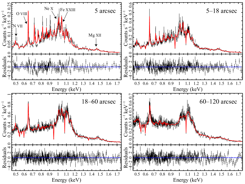
Figure 5: The RGS spectra extracted from each cross-dispersion slice. The black points indicate the data from the observation in 2007 and the red lines are the best-fitting model summarised in Table 2 and 3, where only the first-order spectra are shown for clarity. Several emission line structures are marked on top left panel.

3.2 Abundance Profiles

As described in Section 1, our purpose is to study the central metal distribution in the Centaurus cluster. In Fig. 6, we show radial profiles of elemental abundances except for those of Cr and Mn, which have large statistical uncertainties. The derived abundances of Fe and IMEs show steep negative gradients beyond 120 arcsec from the cluster centre, are peaked at 60–120 arcsec and abrupt drops within the central 18 arcsec. In contrast, O, Ne and Mg have somewhat flatter profiles beyond 120 arcsec. The discrepancies among the abundances from different detectors are significant, about a factor of two at most, especially within the Fe abundance peak. The RGS tends to give lower values of metal abundances than those from the CCDs, with a more significant abundance drop than that with CCDs. These profiles obtained from our analysis are roughly consistent with those from previous works (Panagoulia et al., 2013; Sanders et al., 2016; Liu et al., 2019; Lakhchaura et al., 2019). Moreover, our RGS analysis provides first the Ne abundance profile showing a similar drop with Fe, although there had been no hint of declination of the Ne abundance from works with CCD data (Liu et al., 2019).

As shown in Fig. 7, the abundance ratios to Fe, X/Fe, show flat distributions, although the S/Fe, Ar/Fe, and Ca/Fe ratios within the central 60 arcsec are higher by a few tens of per cent than those beyond 120 arcsec. The scatters in the X/Fe ratios among the different detectors are much smaller than those in the absolute abundances. Exceptionally, RGS and CCDs yield significantly different Ne/Fe ratios. Considering that the Ne-K lines are blended in the Fe-L lines with the CCD as mentioned in § 3.1.1, we expect RGS gives more reliable Ne/Fe ratios. Although the O/Fe ratios with pn are about a factor of two lower than those with MOS, which has a slightly better energy resolution than pn, are consistent with those derived from the RGS spectra. Therefore, for CCSN products of O, Ne, and additionally Mg, we will discuss only the results with RGS data, which would provide a better estimate of these abundances with its high spectral resolution. The Ca/Fe ratios among the CCD detectors show discrepancies of about 50 per cent at most, while the other IMEs/Fe ratios are consistent with each other.

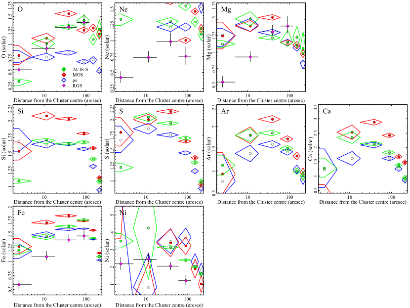
Figure 6: Radial profiles of the metal abundances (O, Ne, Mg, Si, S, Ar, Ca, and Fe) obtained using a triple CIE model. The green-, red-, and blue-diamond plots are for results with Chandra ACIS-S, XMM-Newton MOS, pn, respectively. The magenta plots indicate the RGS results of O, Ne, Mg, Fe, and Ni. We plot the Ne abundance setting the y-axis range according to values with RGS for clarity.

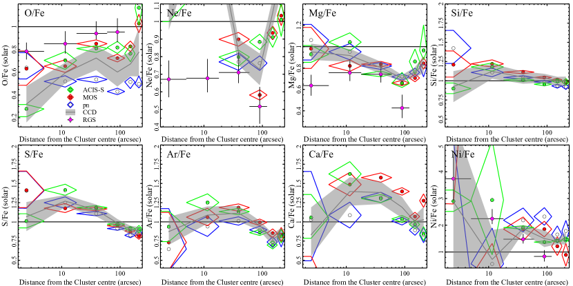
Figure 7: Radial profiles of the relative abundance ratios to Fe obtained using a triple CIE model. The diamonds follow the same manner as Fig 6. The shaded areas indicate the mean values among three CCD detectors. We also show the solar ratio with solid lines on each panel.

3.3 Systematic Uncertainties

Various systematic uncertainties sometimes give biases in abundance measurements in cool cores (e.g., Werner et al., 2008). For example, simple temperature modelling to a complex structure in cores would lead to underestimation of abundances, especially when fitting spectra with strong Fe-L lines (e.g., Buote & Canizares, 1997; Matsushita et al., 2003). Therefore, we also estimate the abundances using other temperature structure models; two and four CIE components. For the four-CIE model, the temperature of the coolest component is half of that of the second coolest one as the temperatures of this model making a geometric sequence with a common ratio of 0.5. Even for the innermost region, these models give almost the same Fe abundances within several per cent with those derived in the previous subsection. Since the quadruple model yields unnaturally low VEM for one component ($<$ 1 per cent of the other three) and almost the same C-statistic values, we conclude that the three temperature-components model is sufficient to model the emission from the Centaurus core.

Projection of X-ray emission along the line of sight could also obscure the actual distribution of temperature or abundances. Since the Centaurus cluster core deviates from spherical symmetry due to the plume-like structure, we do not apply the deprojection method often used to analyse the X-ray emission from cluster cores (e.g., Ettori, 2002; Ikebe et al., 2004; Russell et al., 2008). Instead, we fit the innermost spectra using a sextuple-CIE model. Here, we first fit the spectra of the outermost bin, or 180–240 arcsec region, with a single-CIE model. Then, we fit the spectra of 120–180 arcsec region with a two-CIE model, where one CIE component has the same temperature and metal abundances as those at the outermost region. Finally, we fit the innermost spectra using a sextuple-CIE model. Then, we get almost the same metal abundances within 10 per cent as those with the three-component CIE model.

Next, in order to study the uncertainties caused by systematics in the atomic data, we fit the spectra of the MOS and RGS with the SPEXACT version 3.06.01 (Kaastra et al., 1996). We plot the derived abundances and relative abundance ratios to Fe with AtomDB and SPEXACT in Fig. 8. We do not report the results for Ne in Fig. 8(a) because the Ne-K lines are blended into the Fe-L complex in CCD spectra. With MOS data, the latest version of SPEXACT gives almost the same abundances except for the O abundances. With RGS, SPEXACT yields nearly constant metal abundances in the core, which are significantly different from those with AtomDB (Fig. 8(b)). On the other hand, the abundance ratios with RGS are mostly consistent within a few tens of per cent for all elements between both atomic codes (Fig. 8(c)). The differences of $\sim$ 20 per cent in the O/Fe ratios and Ne/Fe ratios between AtomDB and SPEXACT may be caused by systematic uncertainties in the Fe-L atomic code. We note that the Ne/O ratios with RGS from SPEXACT and AtomDB agree with each other.

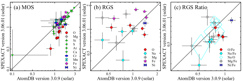
Figure 8: (a) A comparison of the metal abundances (O, Mg, Si, S, Ar, Ca, Fe, Cr, Mn, and Ni) in each annular region of the MOS data with AtomDB version 3.0.9 and SPEXACT version 3.06.01. The Ne abundance is absent in the plots for its unreliability (see § 3.2). For the Cr, Mn, and Ni abundance, we show the averaged values on the central $<$ 120 arcsec core and the outer 120–240 arcsec region. (b) Same as (a) for O, Ne, Mg, Fe, and Ni taken from the RGS data. (c) A comparison of the relative abundance ratios for O/Fe, Ne/Fe, Ne/O, Mg/Fe, and Ni/Fe obtained from the RGS data. The dotted lines shown in each panel indicate the equal value between two codes.

4 DISCUSSION

4.1 Abundance Measurements in the Innermost Regions

As described in Section 1, the mechanisms of the abundance depletions sometimes reported in cluster cores are still under discussion. We also detect abrupt abundance drops within central 18 arcsec for most elements. Panagoulia et al. (2013) and Lakhchaura et al. (2019) proposed that these drops arise from cool dust grains in the cluster centre to which a significant fraction of metals is locked up. If this is the case, we expect that the abundance of non-reactive elements, i.e., the noble gas, show no central drop. Lakhchaura et al. (2019) reported that only the Ar/Fe ratio in the Centaurus cluster core slightly increases towards the centre while the Ar abundance still shows a central drop as other metals. They concluded that the drops are due to the incorporation of metals into dust grains. Our Ar/Fe profile from the longer exposure data also shows a slight increase towards the cluster centre from 120 arcsec and is consistent within error bars with that derived by Lakhchaura et al. (2019). However, we get a flat profile within $\lesssim$ 60 arcsec where the abundance drop occurs (Fig. 7). We note that the increasing profile of the Ar/Fe ratio by Lakhchaura et al. (2019) is partially attributed to their region selection with the $\lesssim$ 30 arcsec innermost bin. This larger radius than ours is suitable for XMM-Newton but probably makes a too much concession to the extremely high angular resolution of the Chandra ACIS ($\sim$ 0.5 arcsec), which could blur the innermost metal distribution in exchange for photon statistics. Our Ar/Fe profile is quite similar to that of the Ca/Fe ratios even though Ca can be easily trapped into dust grains. In addition, we find that the Ne/Fe profile using RGS is also flat towards the centre. These results do not support the grain origin for the abundance drops.

The different detectors and different plasma codes give significantly inconsistent elemental abundances, while the discrepancies in the abundance ratios are relatively small. To investigate the origin of these discrepancies, we fix the Fe abundance at the peak value ($\sim$ 1.7 solar at 60–120 arcsec) and fit the spectra of the innermost region ($<$ 5 arcsec) of RGS and MOS. As shown In Fig. 9, this high Fe abundance model reproduces the continuum and most of the line emissions for both AtomDB and SPEXACT, yielding similar abundance ratios. With AtomDB, the derived C-stat/dof for the RGS spectrum, 5363.8/5663, is significantly larger than 5303.1/5662 with the best-fitting Fe abundance at 0.58 solar. This large C-statistic is mainly caused by residual structures at 1.1–1.2 keV energy band, rather than the difference in the equivalent width of lines. In contrast, as shown In Fig. 9, SPEXACT, which yields the best-fitting Fe abundance of 1.4 solar at the innermost region, does not show such residual structures. When we exclude the 0.9–1.2 keV band where the abovementioned discrepancy between two codes is exhibiting, the derived Fe abundance with AtomDB becomes 1.2$\pm$0.3 solar. This value mostly converges to that with SPEXACT and also that with MOS data, although the Fe abundance with MOS data under the same excision is not significantly changed. Thus, while the Fe abundance drop is not dissolved completely, quite a sharp drop with RGS data could be attenuated. The disagreement between the latest version of AtomDB and SPEXACT occurs for Fe xxiii and Ne x emission lines around 1.2 keV. These deficits around this energy band have been reported since ASCA, especially in luminous X-ray sources like binaries or SN remnants (e.g., Brickhouse et al., 2000; Katsuda et al., 2015; Nakano et al., 2017). We also fit the RGS and MOS spectra at the 60–120 arcsec region in the same way, fixing the Fe abundance at 0.5 and 1.7 solar. Then, as seen in the bottom-right panel of Fig. 9, the low Fe abundance models cannot reproduce the line strength of the Fe line at 6.7 keV.

The systematic uncertainties in the derived abundances from $\sim$ 1 keV plasma have been discussed (e.g., Arimoto et al., 1997; Matsushita et al., 1997, 2000; Mernier et al., 2020a; Gastaldello et al., 2021). The two-photon and free-bound emissions by heavy elements contribute to the continuum, especially for the lower temperature plasma in the innermost regions. Spectral fits try to reduce C-statistics for the lower energy band with high statistics, where the line emissions dominate the continuum. Then, minor systematic uncertainties in the atomic data and/or in the response matrices can bias the derived abundances. The local fits around the Fe-He $\alpha$ line also give abundance drops, where the atomic data is expected to be much more reliable than those for Fe-L lines. This is because the abundances of the other elements are fixed to the best-fitting values from the global fits. For example, when we fix the $\alpha$-elements abundances at 1.3 solar, the local fits for the Chandra $<5$ arcsec region gives the Fe abundance of 1.1 solar. Thus, measurements of absolute abundances are challenging especially in the very core gas, where the abundance drops are reported. In the hot outer regions in which the prominent Fe-K line is detected, the absolute abundances thereof are more reliable. In contrast, the abundance ratios are determined from the ratios of line strengths. As a result, the two atomic codes and different CCDs yield more consistent abundance ratios than the absolute abundances.

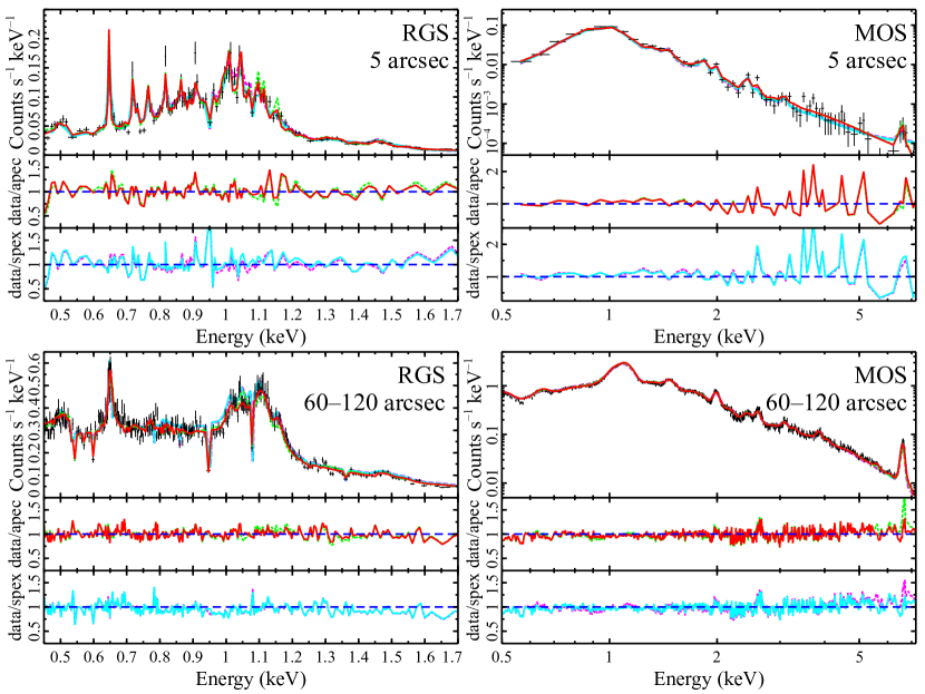
Figure 9: A comparison of two models and atomic codes. The spectra at the innermost region and at the peak of the Fe abundance are plotted for RGS and MOS. The red solid line represents the best-fitting model (Fe $\sim$ 0.5 solar at $<$ 5 arcsec, Fe $\sim$ 1.7 solar at 60–120 arcsec) with AtomDB and the green dotted one is for the fixed Fe abundance model (Fe $=1.7$ solar at $<$ 5 arcsec, Fe $=0.5$ solar at 60–120 arcsec), respectively. The cyan solid and magenta dotted lines follow the same plotting manner but using SPEXACT, where the best-fitting and peak Fe abundances are 1.4 and 1.7 solar, respectively. We also plot the divided data by each model, where data/apec is for the results with AtomDB and data/spex is for SPEXACT.

4.2 Abundance pattern of the Centaurus cluster core

We plot the absolute and relative abundance pattern in the ICM of the Centaurus core (Fig. 10(a) and (b)). Here we use the weighted averages of the derived abundances within ($<$ 18 arcsec) and outside (18–120 arcsec) the abundance drop. Outside the abundance drop, the metal abundances from N to Ni are over-solar values, consistent with previous X-ray studies (e.g., Matsushita et al., 2007; Takahashi et al., 2009; Sakuma et al., 2011; Sanders et al., 2016). These abundances are significantly larger than those observed in the Perseus cluster core with Hitomi (Simionescu et al., 2019), other cool-core systems including groups (Mernier et al., 2018c), and early-type galaxies (Konami et al., 2014). The statistical uncertainties in Cr, Mn, and Ni abundances are comparable to those of the Perseus cluster core (Mernier et al., 2018c; Simionescu et al., 2019). As shown in Fig. 10(b), the abundance ratio pattern in the Centaurus core is mostly consistent with the solar composition and those of other cool-core systems and early-type galaxies (e.g., Mernier et al., 2018c; Simionescu et al., 2019; Konami et al., 2014). The exceptions are the high Ni/Fe ratio, about 1.5–2 solar, with RGS and CCDs, high N/O ratio at 1.5 solar, and low Ne/Fe and Mg/Fe ratios at 0.6 solar with RGS.

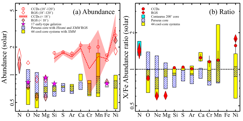
Figure 10: (a) Abundance pattern measured in $<$ 18 arcsec and 18–120 arcsec region of the Centaurus cluster. The open circle and diamond plots show the results of 18–120 arcsec region derived from CCDs and RGS, respectively. The shaded area and filled diamonds are from the central 18 arcsec core with CCDs and RGS, respectively. For comparison, we plot the patterns in the ICM from other works, where the star plots are from 17 early-type galaxies (Konami et al., 2014), the blue boxes are from the Perseus cluster (Simionescu et al., 2019), and the yellow boxes are from 44 cool-core clusters, groups, and ellipticals (CHEERS sample; Mernier et al., 2018c). (b) Abundance ratio pattern obtained from the central 120 arcsec core in the same manner of the left. The cyan box indicates the N/Fe ratio in the Centaurus cluster from Mao et al. (2019), while the blue and yellow boxes are from Simionescu et al. (2019) and Mernier et al. (2018c).

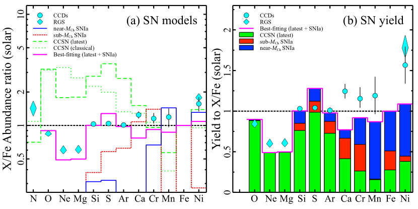
Figure 11: (a) Comparison of the abundance ratio pattern same as Fig. 10(b) with SN nucleosynthesis models. The thin solid, dotted, dashed and dot-dashed lines represent the relative abundance ratios to Fe for near-$M_{\textrm{Ch}}$ SNIa (Leung & Nomoto, 2018), for sub-$M_{\textrm{Ch}}$ SNIa (Shen et al., 2018), for latest CCSN (Sukhbold et al., 2016), and ‘classical’ CCSN (Nomoto et al., 2006), respectively. The magenta thick line corresponds to the best-fitting model which assumes a linear combination of SNIa and latest CCSN model. (b) The contribution of each type of SNe to the best-fitting ratio pattern.

Table 5: Best-fitting combination of CCSN and SNIa yield models by number to the abundance ratio pattern observed in the core of the Centaurus cluster.

SN type	Model	All elements	Excluding Ne, Mg, and Ni
	(Reference)
near-$M_{\textrm{Ch}}$ SNIa	W7	$0.10\pm 0.03$	$0.08\pm 0.04$
	(Leung & Nomoto, 2018)
sub-$M_{\textrm{Ch}}$ SNIa	double detonation	$0.06\pm 0.04$	$0.11\pm 0.06$
	(Shen et al., 2018)
CCSN	N20	$0.84\pm 0.03$	$0.82\pm 0.04$
	(Sukhbold et al., 2016)
$\chi^{2}$/dof		11.2/8	7.2/5
near-$M_{\textrm{Ch}}$ SNIa	W7	$0.03\pm 0.02$	$0.02\pm 0.01$
sub-$M_{\textrm{Ch}}$ SNIa	double detonation	$0.04\pm 0.02$	$0.04\pm 0.02$
CCSN	classical	$0.93\pm 0.02$	$0.94\pm 0.02$
	(Nomoto et al., 2006)
$\chi^{2}$/dof		17.8/8	9.9/5

4.2.1 Contributions from different SN yield models

We consider a linear combination of recent SN nucleosynthesis calculations to reproduce the abundance ratio pattern from the O/Fe to Ni/Fe observed in the Centaurus core. We adopt the latest update of W7 model from 2D hydrodynamics simulations (Leung & Nomoto 2018, for near-$M_{\textrm{Ch}}$ SNIa) and a double-degenerated double-detonation explosion of a solar mass and solar metallicity white dwarf (Shen et al. 2018, for sub-$M_{\textrm{Ch}}$ SNIa). A recent calculation of exploding massive stars averaged over Salpeter initial mass function (Salpeter, 1955) calibrated using observed energy of SN 1987A (N20 model, Sukhbold et al. 2016) and the classical calculations of Nomoto et al. (2006) are considered for CCSN yield models. These models are plotted in Fig. 11(a) with the observed abundance ratio pattern. To fit the pattern and calculate $\chi^{2}$, we consider not only the statistical errors of the observed abundance ratios but also 20 per cent systematic uncertainties reflecting the discrepancies between the derived abundance ratios from AtomDB and SPEXACT. Table 5 summarises the fitting results with the contributions of each SN population to the total number of SNe. The N20 model by Sukhbold et al. (2016) gives a smaller $\chi^{2}$ than the ‘classical’ model by Nomoto et al. (2006). Since the Ne/Fe, Mg/Fe, and Ni/Fe ratios deviate from the best-fitting pattern even using the N20 model, we excluded Ne, Mg, and Ni and fit the abundance pattern in the same way. Then, we get a better $\chi^{2}$, but the contributions of each SN model are consistent within the error bars. The ratio of numbers of CCSN to the total number of SNe is about 80 per cent with the N20 model, while it is about 90 per cent with the ‘classical’ model. This result is consistent with those for the other clusters (e.g., Simionescu et al., 2015; Simionescu et al., 2019). Fig. 11(b) shows the contributions of CCSN, sub-$M_{\textrm{Ch}}$, and near-$M_{\textrm{Ch}}$ SNeIa to each element for the best-fitting combination with the N20 model.

4.2.2 Abundance pattern of $\alpha$-elements

Fig. 11(a) shows that O, Ne, and Mg are predominately synthesised by CCSNe. The discrepancies between the observed O, Ne, and Mg abundance pattern and those by CCSN models significantly contribute to the $\chi^{2}$ in Table 5. The observed O, Ne, and Mg abundance pattern, lower Ne and Mg abundances compared to the O abundance, resembles that of the latest CCSN/N20 model by Sukhbold et al. (2016) rather than the ‘classical’ CCSN model by Nomoto et al. (2006). Fig. 11(b) shows that Si, S, and Ar are mostly synthesised by CCSNe. The combination with the N20 model, near- and sub-$M_{\textrm{Ch}}$ roughly reproduces the observed abundance pattern of these elements and Fe. The contribution of SNeIa products is higher to Ca than those for the other IMEs, although the observed Ca/Fe ratio is significantly higher than the best-fitting combination.

4.2.3 Abundance pattern of Fe-peak elements

The observed Cr/Fe and Mn/Fe pattern is explained by a combination of CCSNe, near-$M_{\textrm{Ch}}$ SNeIa, and sub-$M_{\textrm{Ch}}$ SNeIa, as for the Perseus cluster core. As summarised in Section 1, the Fe-peak elements are mainly forged by SNeIa, especially in the hottest layers of the exploding white dwarf (e.g., Seitenzahl et al., 2013). In particular, ⁵⁵Mn is an important element since it is synthesised more by SNeIa than CCSNe relative to Fe (Kobayashi & Nomoto, 2009), while Cr/Fe and Ni/Fe ratios are less independent of the SNIa/CCSN contributions. As shown in Fig. 11(a), the CCSN models predict the Mn/Fe ratios of approximately a half of the solar ratio. The observed solar Mn/Fe ratio in the Centaurus core and other systems indicate a significant contribution of SNeIa products to the Fe-peak elements. The latest hydrodynamic simulations (e.g., Leung & Nomoto, 2018) predict that the extremely high-density core of near-$M_{\textrm{Ch}}$ SNeIa synthesises a higher fraction of neutronised isotopes like ⁵⁵Mn and ⁵⁸Ni than sub-$M_{\textrm{Ch}}$ ones, which is also confirmed by observational studies on SNIa remnants (e.g., Yamaguchi et al., 2015; Ohshiro et al., 2021). The observed solar Mn/Fe ratio indicates a significant contribution from near-$M_{\textrm{Ch}}$ SNeIa. The observed Cr/Fe ratio is close to the solar ratio like other cool-core systems (e.g., Mernier et al., 2018c). When fitted with a model of either near-$M_{\textrm{Ch}}$ SNIa or sub-$M_{\textrm{Ch}}$ SNeIa with a contribution from CCSNe (N20), the $\chi^{2}$/dof value becomes 14.3/9 and 26.2/9, respectively, favouring both progenitor types of SNIa substantially contributing to the enrichment. The contribution of the sub-$M_{\textrm{Ch}}$ SNeIa is also needed to explain the observed solar Cr/Fe and Mn/Fe pattern.

Although we use the latest atomic code revised after the Hitomi observations of the Perseus core, the observed Ni/Fe ratios of the Centaurus cluster, 1.5–2 times the solar ratio, are significantly higher than the solar ratio of the Perseus cluster core (Simionescu et al., 2019) and the 44 cool-core systems (Mernier et al., 2018c). In our Galaxy, both CCSN and SNIa have synthesised Ni in the same way as Fe, since the Ni/Fe ratio of stars is $\sim$ 1, with no dependence on the Fe abundance (Feltzing & Gustafsson, 1998; Gratton et al., 2003). The observed high Ni/Fe ratio suggests that Ni synthesis in the Centaurus cluster core might be different from that in our Galaxy. However, with CCD detectors, both Ni-L and K lines are blended into the Fe-L lines and He-like Fe-K$\beta$ line at 7.9 keV, respectively, and the derived Ni abundances might be affected by some systematic uncertainties.

4.2.4 Origin of Nitrogen

We also detected the N emission line with RGS within $R_{\textrm{e}}$ of NGC 4696. The weighted average of the observed N/O ratio is $\sim$ 1.5–2 solar in the central 60 arcsec region. As shown in Fig. 11(a), the CCSN nucleosynthesis models predict that the N/O ratio is much less than the solar value. Unlike other light $\alpha$-elements like O and Mg, the N abundance in the cool cores of some galaxy clusters and groups, or in early-type galaxies shows super-solar values, implying a strong chemical contamination by stellar mass loss from asymptotic giant branch (AGB) stars exhibiting in these systems (e.g., Sanders et al., 2008; Mao et al., 2019; Mernier et al., 2022). In Fig. 12, we compare the observed N/O and those expected from AGB yields by Karakas (2010). The observed value is consistent with the calculated ratio assuming AGB stars with low initial mass (1–2 solar) and initial metallicity of solar composition. Thus, the observed N/O ratio indicates the importance of mass loss from low mass AGB stars in the BCG.

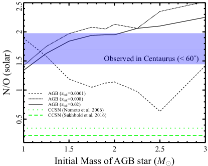
Figure 12: The N/O ratio from AGB stars as a function of initial mass compiled from Karakas (2010), assuming models with several initial metallicity. The shaded area indicates the observed N/O value with RGS in the central 60 arcsec core of the Centaurus cluster. The CCSN yields from Nomoto et al. (2006) and Sukhbold et al. (2016) are also plotted for comparison.

4.3 Comparison with the Stellar Metallicity Profiles

In a cool core, mass loss from AGB stars and SNeIa from the BCG continuously supply metals into the ICM (see Section 1). The former supply metals trapped in stars, which were formed from the ISM enriched by early SNe, and the latter, exploding white dwarfs, pollute the ICM by Fe-peak elements.

In Fig. 13, we plot the stellar metallicity profiles of NGC 4696 by Kobayashi & Arimoto (1999) and the average profiles of stars in early-type galaxies scaled with $R_{\textrm{e}}$ by Kuntschner et al. (2010). Here, we adopt $R_{\textrm{e}}\sim$ 85 arcsec of NGC 4696 (Carollo et al., 1993), and the metallicities are converted using the proto-solar abundance of Lodders et al. (2009). The stellar metallicity of galaxies generally increases towards the centre (Carollo et al., 1993). At the effective radii, the stellar metallicity of $\alpha$-elements of these galaxies are typically close to the solar value, although the accurate metallicity could be different by a factor of two because of high uncertainty and poor understanding in converts to the metalicity of Mg or Fe from strength and depth of optical absorption lines (Kobayashi & Arimoto, 1999).

In Fig. 13, we also plot the Mg and Fe profiles in the ICM of the Centaurus cluster derived from the RGS observations. As described in the previous subsection, at $R_{\textrm{e}}$ of the BCG, the accurate abundances are more reliable than the innermost regions. We found that the Mg abundances derived from X-ray measurements around $R_{\textrm{e}}$ are consistent with the stellar Mg metallicity. At the inner regions, if we adopt the high Fe abundance model without the abundance drop described in § 4.1, i.e. the model with Fe $\sim$ 1.7 solar, the Mg abundances with AtomDB and SPEXACT increase to $\sim$ 1 solar, and becomes consistent with the stellar metallicity as shown in Fig. 13.

When integrating the electron density derived from the VEM profiles out to 120 arcsec, the hot gas mass becomes 7$\times 10^{10}\,\textrm{M}_{\odot}$. This mass is orders of magnitude higher than those in early-type galaxies. For example, that of a massive elliptical galaxy NGC 1404 is only $\sim 7\times 10^{8}\,\textrm{M}_{\odot}$ (Mernier et al., 2022). Considering the $K$-band luminosity of NGC 4696 is 1.8$\times 10^{12}\,\textrm{L}_{\odot}$, and stellar mass-to-light ratio with $K$-band of giant early-type galaxies are around unity (e.g., Nagino & Matsushita, 2009), this gas mass is about 4 per cent of the stellar mass of the BCG. Given that stars lose 10–20 per cent of the initial mass via stellar mass loss over the Hubble time (e.g. Courteau et al., 2014; Hopkins et al., 2022), the accumulating time of the mass loss of NGC 4696 may be much longer than those of early-type galaxies while early mass-loss products would have been lost. Adopting the injection rate of stellar winds from Ciotti et al. (1991), which is $\sim 1.3\,(t/t_{\textrm{now}})^{-1.3}\,\textrm{M}_{\odot}$ yr^-1 in NGC 4696, and assuming star formation epoch, for instance, at 2.5 Gyr ($z\sim$ 2.5, the peak star formation is at $z=$ 2–3, e.g., Madau et al. 1996; Brandt & Hasinger 2005), the time to congregate the observed ICM mass in the central 120 arcsec region is about 9–10 Gyr. We found no significant change in this estimated time when adopting different star formation epochs $z=2$ and $z=3$. In contrast, such a long accumulating time could strongly overestimate the gas mass in normal early-type galaxies (e.g., Mernier et al., 2022). Since we compare abundances in stars and ICM which could have very different histories from each other, the actual accumulation time may change from our simple or simplistic estimation. For the other clusters with more luminous cool cores, with higher ICM masses and lower metal abundances, it may be difficult to explain the observed $\alpha$-elements peak with stellar mass loss (e.g. de Plaa et al., 2006; Simionescu et al., 2009; Mernier et al., 2017).

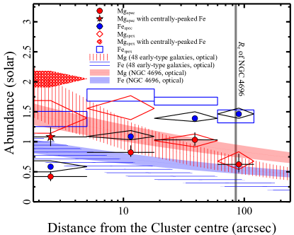
Figure 13: The abundance profile of Mg (red) and Fe (blue) overlaid with the stellar metallicity observed in early-type galaxies (hatched strips, Kuntschner et al. 2010) and NGC 4696 (shaded strips, Kobayashi & Arimoto 1999).

4.4 Fe mass and SNIa rate

While the total gas mass in the Centaurus core can be accounted for by the mass ejection through stellar winds (see § 4.3), how about the masses of each element, especially for Fe? As shown in Fig. 13, the Fe abundances in the ICM are significantly higher than the stellar Fe metallicity, especially around $R_{\textrm{e}}$ of the BCG, where the absolute abundances are relatively reliable. In addition, the Mg/Fe ratios in the ICM are also different from the super-solar $\alpha$/Fe ratios of stars in giant early-type galaxies (e.g., Kobayashi & Arimoto, 1999; Kuntschner et al., 2010). These results strongly suggest the additional enrichment of Fe by SNeIa. Then, the Fe abundances in the ISM can constrain the past metal supply by SNeIa. Adopting the stellar Fe metallicity of $\sim$ 0.5 solar, the Fe abundance synthesised by SNeIa becomes $\sim$ 1 solar. From the derived electron density and Fe abundance profiles, the total Fe mass from SNeIa in the ICM out to 120 arcsec becomes $(1.1\pm 0.2)\times 10^{8}$ $\textrm{M}_{\odot}$. We note that the Fe mass ejected from the stellar population with the metallicity in Fig. 13 is about $6\times 10^{7}\,\textrm{M}_{\odot}$ which is a factor of two lower than the observed Fe mass.

The present metal supply by SNeIa can be studied using the Fe abundance in the ISM in early-type galaxies. The mass of the hot ISM in giant early-type galaxies are typically less than 1 per cent of stellar mass and the timescale for accumulation of the hot ISM is smaller than $\sim$ 1 Gyr (Matsushita, 2001). At a given epoch, the absolute abundance of Fe synthesised by SNeIa is calculated by

$$M^{\textrm{Fe}}_{\textrm{SNIa}}\frac{\theta_{\textrm{SNIa}}}{\alpha_{\ast}z^{\textrm{Fe}}_{\textrm{solar}}}$$ (1)

Detailed discussion for equation (1) is given in Matsushita et al. (2003). Here, $M^{\textrm{Fe}}_{\textrm{SNIa}}$, the Fe mass forged by one SNIa, is $\sim 0.5$–$0.7\,\textrm{M}_{\odot}$ (e.g., Iwamoto et al., 1999; Seitenzahl et al., 2013; Shen et al., 2018; Leung & Nomoto, 2018), $\theta_{\textrm{SNIa}}$ is the SNIa rate, $\alpha_{\ast}$ is the stellar mass-loss rate, and $z^{\textrm{Fe}}_{\textrm{solar}}\sim$ 0.001 is the solar Fe mass fraction. The optical observed rate of SNeIa is 0.1–0.4 SNIa (100 yr $10^{10}\,\textrm{L}_{B,\odot}$)^-1 (e.g., Li et al., 2011). Using the injection rate of stellar wind by Ciotti et al. (1991), the expected Fe abundance from SNeIa in the hot ISM in early-type galaxies is at least 2 solar (e.g., Matsushita et al., 2000; Konami et al., 2014). However, the observed Fe abundances in the ISM of early-type galaxies with Suzaku are about 1 solar (e.g., Konami et al., 2014). Since the temperatures of the hot ISM in early-type galaxies are close to that of the ICM in the innermost region of the Centaurus cluster, there may be some systematic uncertainties in the derived metal abundances in the ISM.

The Fe abundance in the ICM at the Fe-peak of the Centaurus cluster is significantly higher than those in the hot ISM in early-type galaxies. We integrated the stellar mass-loss rate and SNIa rate over the past 9–10 Gyr, using the mass-loss rate by Ciotti et al. (1991) and the delay-time distribution of SNIa rate modelled by a power-law behaviour ($\propto t^{-1.34}$, Heringer et al. 2019). Assuming star formation at 2.5 Gyr ($z\sim$ 2.5), the present SNIa rate is estimated to be 0.11 SNIa (100 yr $10^{10}\,\textrm{L}_{B,\odot}$)^-1 in order to produce the entire Fe mass observed in the core over the past 9–10 Gyr. This value is marginally consistent with the SNeIa rate by the optical observations (Li et al., 2011). When applying star formation at $z=2$ and $z=3$, we did not find remarkable changes in these results.

The ratio of the ICM mass to the stellar mass in the core of the Centaurus cluster ($\sim$ 4 per cent) is a few orders of magnitude higher than those in early-type galaxies, indicating a longer enrichment time scale (see § 4.3). In contrast, the iron-mass-to-light ratio of the Centaurus cluster core ($\sim 10^{-5}\,\textrm{M}_{\odot}/\textrm{L}_{K,\odot}$) is much lower than those of clusters of galaxies ($\sim 10^{-3}\,\textrm{M}_{\odot}/\textrm{L}_{K,\odot}$, Matsushita et al. 2013a, b). Our discussed enrichments by SNeIa and/or stellar winds would suggest a relatively recent or even an ongoing enrichment scenario in the Centaurus core. However, such a recent enrichment scenario hardly explains the uniform and solar X/Fe ratio (in early-type galaxies, the Centaurus core, and other clusters) unless SNeIa and stellar winds have been sophisticatedly controlled to reproduce the observed abundance pattern, which might be a handiwork. Recently, Mernier et al. (2022) discussed that the abundance patterns observed in cluster or galaxy centres are more likely produced by an early enrichment which would have started at $z\sim 3$ and ended around $z=2$. If this is the case, enrichment channels must be CCSNe, the earliest SNeIa, and stellar winds whose rates are more difficult to be estimated accurately than those at the present. We also note that such an early enrichment scenario would be challenged by the escaping or depleting metals that must have been produced subsequently unless the recent SNeIa and stellar winds are completely quiescent. Further studies of metal abundance, distribution, and cycle process, not only at central cores but also at large scales will provide important clues to solving this cosmic conundrum.

4.5 Future prospects

Future X-ray mission with high-resolution and spatially resolved spectroscopy like XRISM is more crucial to reduce the systematic uncertainties and to estimate the absolute abundance in the cool innermost region of clusters. Since the observational data, the nucleosynthesis theories, and the atomic codes are limited at present, we comprehend, as also discussed in § 4.1, the necessity of extremely high-resolution spectra with micro-calorimeter detectors onboard future missions like XRISM (XRISM Science Team, 2020) or Athena (e.g., Cucchetti et al., 2018; Mernier et al., 2020b). For example, the Resolve instrument, which will be mounted on XRISM and deliver a constant $<7$ eV spectral resolution, enables us to fully resolve the Ne K-shell emission line from the Fe-L complex. Offering its non-dispersive X-ray spectroscopy, Resolve provides more accurate spatial information of emission lines in the cluster and group centres than those with the RGS data. By using the low-temperature region of these targets with laboratory experiments (e.g., electron beam ion traps, Gu et al. 2020), we expect that the remaining uncertainties or disagreements between AtomDB and SPEXACT will continue to be reduced. In particular, our proposed disagreement in the $0.9$–$1.2$ keV band, possibly attributed to mismodelling of the Fe xxiii and Ne x emission lines (see § 4.1), will be an urgent issue to be resolved. Based on these upcoming leaps, XRISM and/or Athena will provide crucial knowledge of metal content in the cluster or group centres, including the abundance drop, as discussed in Gastaldello et al. (2021).

Furthermore, it is important that the trace odd-$Z$ elements other than N could also be a sensitive diagnostic of the initial metallicity of CCSN progenitors (e.g., Nomoto et al., 2006; Nomoto et al., 2013) or of the stellar population (e.g., Campbell & Lattanzio, 2008; Karakas, 2010). Unfortunately, we are not able to constrain the abundance of these elements while using present grating data. The micro-calorimeter instruments mounted on Hitomi have been shown enough resolution and sensitivity to constrain the abundance of trace odd-$Z$ elements (e.g., Simionescu et al., 2019), which makes us expect invaluable information about the underlying stellar population contributing to the early enrichment history of the ICM.

5 CONCLUSIONS

The elemental abundances in the cluster cool cores provide a key to understanding the chemical enrichment of the central BCG and the surrounding ICM. We report the detailed distributions of elements in the ICM expelled by SNe using the deep Chandra and XMM-Newton observations of the cool core of the Centaurus cluster of galaxies. While the abundance drop in the innermost region is observed as previous studies (e.g., Panagoulia et al., 2013; Lakhchaura et al., 2019; Liu et al., 2019), we find that the relative abundance ratios to Fe yield flat profiles towards the centre, even for noble gas elements, Ne/Fe and Ar/Fe. In addition, a much higher Fe abundance model without an abundance drop also reproduces the spectra of the innermost region, excluding the Fe-L complex around 1.2 keV with ATOMDB. These results suggest that the abundance drop may be at least partly artificially caused by some systematic uncertainties in the atomic data and/or response matrices, rather than the metal depletion process on to the cold dust grains.

The measured abundance pattern shows that the Si/Fe, S/Fe, Ar/Fe, Ca/Fe, Cr/Fe, and Mn/Fe ratios are close to the solar values. On the other hand, the O/Fe, Ne/Fe, and Mg/Fe ratios tend to be lower ($\sim$ 0.6–0.9 solar) and the N/Fe ratio is higher ($\sim$ 1.5 solar). Even using the latest versions of atomic code, the Ni/Fe ratio ($\sim$ 2 solar) is significantly higher than the solar ratio and that of the Perseus core (Simionescu et al., 2019). Taking the systematic uncertainties (e.g., atomic codes) into account, we test linear combination models of recent SN yield calculations for near- and sub-$M_{\textrm{Ch}}$ SNIa (Leung & Nomoto 2018 and Shen et al. 2018, respectively), and CCSN (N20, Sukhbold et al. 2016; ‘classical’, Nomoto et al. 2006) in order to reproduce these abundance ratios. We find that the contribution of both near- and sub-$M_{\textrm{Ch}}$ SNIa is needed to explain the Cr/Fe and Mn/Fe (and possibly Ni/Fe) ratios. The number ratio of CCSNe to the total SNe contributing to the enrichment is 80 per cent with the latest N20 model and 90 per cent with the ‘classical’ calculation, consistent with the estimated values in other clusters (e.g., Simionescu et al., 2015). None the less, the low Ne/Fe and Mg/Fe ratios and the high Ni/Fe ratio are not reproduced satisfactorily by our linear combination models of each SN population.

Since the N enrichment through SNIa and CCSN is measly, we compare the observed N/O abundance ratio ($\sim$ 1.7 solar with RGS) in the cool core with the calculated values in stellar winds from AGB stars. We find that the observed N/O ratio is consistent with the values expected in winds from AGBs with a low initial mass ($\sim 1\textrm{M}_{\odot}$). The derived Mg abundance around NGC 4696 is comparable to the stellar metallicity observed in early-type galaxies with optical observations (Kobayashi & Arimoto, 1999; Kuntschner et al., 2010). These results for the abundance of lighter elements imply the gas expelled by stellar mass loss is dominant around NGC 4696. The ICM mass within the central 120 arcsec core can be reproduced over the last 9–10 Gyr enrichment time of stellar mass loss, assuming a star formation at $z=$ 2–3. Adopting the power-law delay-time distribution of SNIa rate and accumulating it over the past 9–10 Gyr, the present SNIa rate required to reproduce the central Fe mass is 0.11 SNIa (100 yr $10^{10}\,\textrm{L}_{B,\odot}$)^-1. This value is marginally consistent with the rate reported by optical observations (e.g., Li et al., 2011).

This study also shows that the high-resolution spectroscopy is important to measure the metal abundances and to reveal the chemical enrichment in the cooler innermost region of clusters. Future missions are crucial to obtain a more precise picture of the chemical enrichment and evolutionary history of clusters of galaxies with robust constraints on element abundances especially of Fe-peak and trace odd-$Z$ elements.

Data Availability

The Chandra data used in this work are publicly available from the Chandra X-ray Center (https://cda.harvard.edu/chaser/). The XMM-Newton Science Archive (http://nxsa.esac.esa.int/nxsa-web/) stores the observational data used in this paper, which can be downloaded through the High Energy Astrophysics Science Archive Research Center (HEASARC). The software packages heasoft and xspec were used, and these can be downloaded from the HEASARC software web page (https://heasarc.gsfc.nasa.gov/docs/software/). The figures in this paper were created using veusz (https://veusz.github.io/) and python version 3.7.

References

- Allen & Fabian (1994) Allen S. W., Fabian A. C., 1994, MNRAS, 269, 409
- Arimoto et al. (1997) Arimoto N., Matsushita K., Ishimaru Y., Ohashi T., Renzini A., 1997, ApJ, 477, 128
- Arnaud (1996) Arnaud K. A., 1996, in Jacoby G. H., Barnes J., eds, Astronomical Society of the Pacific Conference Series Vol. 101, Astronomical Data Analysis Software and Systems V. p. 17
- Biffi et al. (2018) Biffi V., Mernier F., Medvedev P., 2018, Space Sci. Rev., 214, 123
- Böhringer et al. (2004) Böhringer H., Matsushita K., Churazov E., Finoguenov A., Ikebe Y., 2004, A&A, 416, L21
- Brandt & Hasinger (2005) Brandt W. N., Hasinger G., 2005, ARA&A, 43, 827
- Brickhouse et al. (2000) Brickhouse N. S., Dupree A. K., Edgar R. J., Liedahl D. A., Drake S. A., White N. E., Singh K. P., 2000, ApJ, 530, 387
- Buote & Canizares (1997) Buote D. A., Canizares C. R., 1997, ApJ, 474, 650
- Campbell & Lattanzio (2008) Campbell S. W., Lattanzio J. C., 2008, A&A, 490, 769
- Carollo et al. (1993) Carollo C. M., Danziger I. J., Buson L., 1993, MNRAS, 265, 553
- Cash (1979) Cash W., 1979, ApJ, 228, 939
- Chen et al. (2018) Chen Y., Wang Q. D., Zhang G.-Y., Zhang S., Ji L., 2018, ApJ, 861, 138
- Churazov et al. (2003) Churazov E., Forman W., Jones C., Böhringer H., 2003, ApJ, 590, 225
- Ciotti et al. (1991) Ciotti L., D’Ercole A., Pellegrini S., Renzini A., 1991, ApJ, 376, 380
- Courteau et al. (2014) Courteau S., et al., 2014, Reviews of Modern Physics, 86, 47
- Crawford et al. (2005) Crawford C. S., Hatch N. A., Fabian A. C., Sanders J. S., 2005, MNRAS, 363, 216
- Cucchetti et al. (2018) Cucchetti E., et al., 2018, A&A, 620, A173
- De Grandi & Molendi (2001) De Grandi S., Molendi S., 2001, ApJ, 551, 153
- Erdim et al. (2021) Erdim M. K., Ezer C., Ünver O., Hazar F., Hudaverdi M., 2021, MNRAS, 508, 3337
- Ettori (2002) Ettori S., 2002, MNRAS, 330, 971
- Feltzing & Gustafsson (1998) Feltzing S., Gustafsson B., 1998, A&AS, 129, 237
- Foster et al. (2012) Foster A. R., Ji L., Smith R. K., Brickhouse N. S., 2012, ApJ, 756, 128
- Fruscione et al. (2006) Fruscione A., et al., 2006, in Proc. SPIE. p. 62701V, doi:10.1117/12.671760
- Fukazawa et al. (1994) Fukazawa Y., Ohashi T., Fabian A. C., Canizares C. R., Ikebe Y., Makishima K., Mushotzky R. F., Yamashita K., 1994, PASJ, 46, L55
- Gastaldello et al. (2021) Gastaldello F., Simionescu A., Mernier F., Biffi V., Gaspari M., Sato K., Matsushita K., 2021, Universe, 7, 208
- Gratton et al. (2003) Gratton R. G., Carretta E., Claudi R., Lucatello S., Barbieri M., 2003, A&A, 404, 187
- Gu et al. (2020) Gu L., et al., 2020, A&A, 641, A93
- Heringer et al. (2019) Heringer E., Pritchet C., van Kerkwijk M. H., 2019, ApJ, 882, 52
- Hitomi Collaboration et al. (2017) Hitomi Collaboration et al., 2017, Nature, 551, 478
- Hitomi Collaboration et al. (2018a) Hitomi Collaboration et al., 2018a, PASJ, 70, 11
- Hitomi Collaboration et al. (2018b) Hitomi Collaboration et al., 2018b, PASJ, 70, 12
- Hopkins et al. (2022) Hopkins P. F., et al., 2022, arXiv e-prints, p. arXiv:2203.00040
- Ikebe et al. (2004) Ikebe Y., Böhringer H., Kitayama T., 2004, ApJ, 611, 175
- Iwamoto et al. (1999) Iwamoto K., Brachwitz F., Nomoto K., Kishimoto N., Umeda H., Hix W. R., Thielemann F.-K., 1999, ApJS, 125, 439
- Johnstone et al. (2002) Johnstone R. M., Allen S. W., Fabian A. C., Sanders J. S., 2002, MNRAS, 336, 299
- Kaastra (2017) Kaastra J. S., 2017, A&A, 605, A51
- Kaastra et al. (1996) Kaastra J. S., Mewe R., Nieuwenhuijzen H., 1996, in UV and X-ray Spectroscopy of Astrophysical and Laboratory Plasmas. pp 411–414
- Karakas (2010) Karakas A. I., 2010, MNRAS, 403, 1413
- Katsuda et al. (2015) Katsuda S., et al., 2015, ApJ, 808, 49
- Kobayashi & Arimoto (1999) Kobayashi C., Arimoto N., 1999, ApJ, 527, 573
- Kobayashi & Nomoto (2009) Kobayashi C., Nomoto K., 2009, ApJ, 707, 1466
- Konami et al. (2014) Konami S., Matsushita K., Nagino R., Tamagawa T., 2014, ApJ, 783, 8
- Kuntschner et al. (2010) Kuntschner H., et al., 2010, MNRAS, 408, 97
- Lakhchaura et al. (2019) Lakhchaura K., Mernier F., Werner N., 2019, A&A, 623, A17
- Leccardi & Molendi (2008) Leccardi A., Molendi S., 2008, A&A, 486, 359
- Leung & Nomoto (2018) Leung S.-C., Nomoto K., 2018, ApJ, 861, 143
- Li et al. (2011) Li W., et al., 2011, MNRAS, 412, 1441
- Liu et al. (2019) Liu A., Zhai M., Tozzi P., 2019, MNRAS, 485, 1651
- Lodders et al. (2009) Lodders K., Palme H., Gail H. P., 2009, Landolt Börnstein, 4B, 712
- Madau et al. (1996) Madau P., Ferguson H. C., Dickinson M. E., Giavalisco M., Steidel C. C., Fruchter A., 1996, MNRAS, 283, 1388
- Mao et al. (2019) Mao J., et al., 2019, A&A, 621, A9
- Matsushita (2001) Matsushita K., 2001, ApJ, 547, 693
- Matsushita (2011) Matsushita K., 2011, A&A, 527, A134
- Matsushita et al. (1997) Matsushita K., Makishima K., Rokutanda E., Yamasaki N. Y., Ohashi T., 1997, ApJ, 488, L125
- Matsushita et al. (2000) Matsushita K., Ohashi T., Makishima K., 2000, PASJ, 52, 685
- Matsushita et al. (2003) Matsushita K., Finoguenov A., Böhringer H., 2003, A&A, 401, 443
- Matsushita et al. (2007) Matsushita K., Böhringer H., Takahashi I., Ikebe Y., 2007, A&A, 462, 953
- Matsushita et al. (2013a) Matsushita K., Sato T., Sakuma E., Sato K., 2013a, PASJ, 65, 10
- Matsushita et al. (2013b) Matsushita K., Sakuma E., Sasaki T., Sato K., Simionescu A., 2013b, ApJ, 764, 147
- Mernier et al. (2015) Mernier F., de Plaa J., Lovisari L., Pinto C., Zhang Y. Y., Kaastra J. S., Werner N., Simionescu A., 2015, A&A, 575, A37
- Mernier et al. (2017) Mernier F., et al., 2017, A&A, 603, A80
- Mernier et al. (2018a) Mernier F., et al., 2018a, Space Sci. Rev., 214, 129
- Mernier et al. (2018b) Mernier F., et al., 2018b, MNRAS, 478, L116
- Mernier et al. (2018c) Mernier F., et al., 2018c, MNRAS, 480, L95
- Mernier et al. (2020a) Mernier F., et al., 2020a, Astronomische Nachrichten, 341, 203
- Mernier et al. (2020b) Mernier F., et al., 2020b, A&A, 642, A90
- Mernier et al. (2022) Mernier F., et al., 2022, MNRAS, 511, 3159
- Million et al. (2011) Million E. T., Werner N., Simionescu A., Allen S. W., 2011, MNRAS, 418, 2744
- Mittal et al. (2011) Mittal R., et al., 2011, MNRAS, 418, 2386
- Nagino & Matsushita (2009) Nagino R., Matsushita K., 2009, A&A, 501, 157
- Nakano et al. (2017) Nakano T., Murakami H., Furuta Y., Enoto T., Masuyama M., Shigeyama T., Makishima K., 2017, PASJ, 69, 40
- Nakashima et al. (2018) Nakashima S., Inoue Y., Yamasaki N., Sofue Y., Kataoka J., Sakai K., 2018, ApJ, 862, 34
- Nomoto et al. (2006) Nomoto K., Tominaga N., Umeda H., Kobayashi C., Maeda K., 2006, Nuclear Phys. A, 777, 424
- Nomoto et al. (2013) Nomoto K., Kobayashi C., Tominaga N., 2013, ARA&A, 51, 457
- Ohshiro et al. (2021) Ohshiro Y., et al., 2021, ApJ, 913, L34
- Panagoulia et al. (2013) Panagoulia E. K., Fabian A. C., Sanders J. S., 2013, MNRAS, 433, 3290
- Panagoulia et al. (2015) Panagoulia E. K., Sanders J. S., Fabian A. C., 2015, MNRAS, 447, 417
- Russell et al. (2008) Russell H. R., Sanders J. S., Fabian A. C., 2008, MNRAS, 390, 1207
- Sakuma et al. (2011) Sakuma E., Ota N., Sato K., Sato T., Matsushita K., 2011, PASJ, 63, S979
- Salpeter (1955) Salpeter E. E., 1955, ApJ, 121, 161
- Sanders & Fabian (2002) Sanders J. S., Fabian A. C., 2002, MNRAS, 331, 273
- Sanders et al. (2008) Sanders J. S., Fabian A. C., Allen S. W., Morris R. G., Graham J., Johnstone R. M., 2008, MNRAS, 385, 1186
- Sanders et al. (2016) Sanders J. S., et al., 2016, MNRAS, 457, 82
- Sato et al. (2007) Sato K., Tokoi K., Matsushita K., Ishisaki Y., Yamasaki N. Y., Ishida M., Ohashi T., 2007, ApJ, 667, L41
- Seitenzahl et al. (2013) Seitenzahl I. R., et al., 2013, MNRAS, 429, 1156
- Shen et al. (2018) Shen K. J., Kasen D., Miles B. J., Townsley D. M., 2018, ApJ, 854, 52
- Simionescu et al. (2009) Simionescu A., Werner N., Böhringer H., Kaastra J. S., Finoguenov A., Brüggen M., Nulsen P. E. J., 2009, A&A, 493, 409
- Simionescu et al. (2015) Simionescu A., Werner N., Urban O., Allen S. W., Ichinohe Y., Zhuravleva I., 2015, ApJ, 811, L25
- Simionescu et al. (2019) Simionescu A., et al., 2019, MNRAS, 483, 1701
- Struble & Rood (1999) Struble M. F., Rood H. J., 1999, ApJS, 125, 35
- Strüder et al. (2001) Strüder L., et al., 2001, A&A, 365, L18
- Sukhbold et al. (2016) Sukhbold T., Ertl T., Woosley S. E., Brown J. M., Janka H. T., 2016, ApJ, 821, 38
- Takahashi et al. (2009) Takahashi I., et al., 2009, ApJ, 701, 377
- Turner et al. (2001) Turner M. J. L., et al., 2001, A&A, 365, L27
- Urban et al. (2017) Urban O., Werner N., Allen S. W., Simionescu A., Mantz A., 2017, MNRAS, 470, 4583
- Verner et al. (1996) Verner D. A., Ferland G. J., Korista K. T., Yakovlev D. G., 1996, ApJ, 465, 487
- Weisskopf et al. (2002) Weisskopf M. C., Brinkman B., Canizares C., Garmire G., Murray S., Van Speybroeck L. P., 2002, PASP, 114, 1
- Werner et al. (2008) Werner N., Durret F., Ohashi T., Schindler S., Wiersma R. P. C., 2008, Space Sci. Rev., 134, 337
- Werner et al. (2013) Werner N., Urban O., Simionescu A., Allen S. W., 2013, Nature, 502, 656
- Willingale et al. (2013) Willingale R., Starling R. L. C., Beardmore A. P., Tanvir N. R., O’Brien P. T., 2013, MNRAS, 431, 394
- XRISM Science Team (2020) XRISM Science Team 2020, arXiv e-prints, p. arXiv:2003.04962
- Yamaguchi et al. (2015) Yamaguchi H., et al., 2015, ApJ, 801, L31
- Yoshino et al. (2009) Yoshino T., et al., 2009, PASJ, 61, 805
- Zhang et al. (2019) Zhang S., Wang Q. D., Foster A. R., Sun W., Li Z., Ji L., 2019, ApJ, 885, 157
- de Plaa et al. (2006) de Plaa J., et al., 2006, A&A, 452, 397
- de Plaa et al. (2007) de Plaa J., Werner N., Bleeker J. A. M., Vink J., Kaastra J. S., Méndez M., 2007, A&A, 465, 345
- den Herder et al. (2001) den Herder J. W., et al., 2001, A&A, 365, L7