Reliable Flight Control: Gravity-Compensation-First Principle

Abstract

Safety is always the priority in aviation. However, current state-of-the-art passive fault-tolerant control is too conservative to use; current state-of-the-art active fault-tolerant control requires time to perform fault detection and diagnosis, and control switching. But it may be later to recover impaired aircraft. Most designs depend on failures determined as a priori and cannot deal with fault, causing the original system’s state to be uncontrollable. However, experienced human pilots can save a serve impaired aircraft as far as they can. Motivated by this, this paper develops a principle to try to explain human pilot behavior behind, coined the gravity-compensation-first principle. This further supports reliable flight control for aircraft such as quadcopters and tail-sitter unmanned aerial vehicles.

I Introduction

Considerable attention has recently been gained to Fault-tolerant control (FTC) in recent years because of its important role in maintaining the systems’ safety via configured redundancy [1]. FTC is roughly classified into passive FTC and active FTC. The control structure of a passive FTC system will not be changed in both normal and abnormal conditions without performing real-time management of redundancies. This is because the system redundancy has already been integrated into the controller design. In an active FTC scheme, fault detection and diagnosis (FDD) has to be performed via the information from the monitoring system, based on which control algorithms as well as manage redundancies are reconfigured to make the system safe in abnormal conditions. From above, the active FTCs have three main steps: (1) FDD; (2) reconfigurable control; and (3) integration of FDD and reconfigurable control. FDD plays an important and essential role, but it imposes a severe burden on computation, and its delay can adversely affect system safety. Compared with the active FTC, the fault-tolerant ability of the passive FTC is more conservative. Still, its inherent feature of no FDD and controller switching is significant for flight control systems, usually having a minimal amount of time to be recovered.

Most FTC approaches focus on modifying the inner loop of a flight control system [2]. However, an impaired aircraft may have significant restrictions on both its maneuvering capability and the flight envelope or lose its original controllability through which it can be safely controlled. However, the human pilot, who has sometimes developed very innovative strategies to control impaired aircraft, can deal with these issues. First, let us study an accident shown in Fig.1, where a fixed-wing aircraft lost its right-wing in the air at 16s in the video. Since then, the aircraft cannot perform its normal flight task anymore. Instead, the aircraft dropped height and started rolling. At 35s, the nose of the aircraft pointed upward, and its rotation was stopped. From then on, the nose of the aircraft always pointed upward until it approached the ground. At 48s, the aircraft changed its attitude by its left aileron to land on the ground with its wheels. Otherwise, it will sit on the ground with its tail.

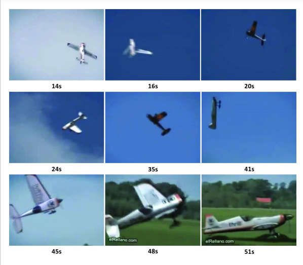
Figure 1: A fixed-wing aircraft lost its right wing in the air

The pilot, we guess, did not have such an experience in dealing with the accident, but the pilot landed the damaged aircraft safely. This is similar to another accident on May 1, 1983, where an Israeli Air Force (IAF) F-15 Baz (actually the F-15D No. 957) collided with an A-4 Skyhawk in an air combat training mission over the Negev. However, the two accidents are very different. The Israeli pilot was able to maintain control because of the lift generated by the large areas of the fuselage, stabilators, and remaining wing. However, the pilot in Fig.1 could not control the aircraft’s attitude anymore.

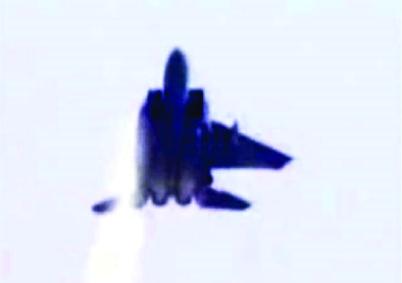
Figure 2: A F-15 lost its most right-wing in the air

From the two accidents, we can learn three control properties from sophisticated pilots:

• Property 1. Such a failure is not defined and analyzed a priori. In practice, it is impossible and tedious to determine all failures.

• Property 2. FDD is unavailable. In the accident shown in Fig.2, the pilot was later quoted as saying, “(I) probably would have ejected if I knew what had happened”. In practice, some faults are also unobservable. On the other hand, this implies that the impaired model is unavailable for controllers. An approach for dealing with this is to automatically optimize or reshape the trajectory of an impaired aircraft for particular tasks in a way that takes any impairment into account [2]. However, this method heavily depends on the impaired model.

• Property 3. More importantly, although the damage caused the aircraft’s attitude to be uncontrollable in the accident shown in Fig.1, the damaged aircraft was landed as safely as possible. As the matter current is either passive or active FTC, the faulty system is often assumed to state controllable as the same as the original system implicitly. To clarify, if a fault causes the original system’s state to be uncontrollable, then we call it a ‘disaster’. Under disasters, pilots always try their best to land a damaged aircraft within a minimal time, rather than care whether the aircraft is controllable.

The three properties motivate us to find the control principle behind it. With the principle, we aim to develop a new flight-control framework with Properties 1-3 to improve the reliability and safety of an aircraft.

In this paper, the gravity-compensation-first principle is proposed from the first principle. We will formulate the principle in three aspects: force, impulse, and energy. With the principle, we study passive disaster-tolerant control of multicopters and fixed-wing using the model predictive control approach.

II Gravity-Compensation-First Principle

II-A Gravity-Compensation-First Principle

According to Newton’s second law, we have

$$\mathbf{\dot{p}} =\mathbf{v}$$

$$\mathbf{\dot{v}} =\mathbf{g+}\frac{1}{m}\mathbf{f}$$ (1)

where $\mathbf{p,v}\in\mathbf{\mathbb{R}}^{3}$ are position and velocity of an aircraft, $\mathbf{g}\in\mathbf{\mathbb{R}}^{3}$ is acceleration of gravity, $m\in\mathbf{\mathbb{R}}$ is mass of the aircraft, $\mathbf{f}\in\mathbf{\mathcal{F}}\subset\mathbf{\mathbb{R}}^{3}$ is the force on the aircraft other than gravity. As shown in Fig.3, the function of the nose of the aircraft pointing upward aims at decreasing falling speed, which is a significant change the pilot made around 35s. After that, the falling speed is under control. This is a crucial step to why the pilot can survive the accident. Also, this implies that compensating for gravity is the first requirement.

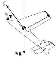
Figure 3: The nose of the aircraft pointing upward to compensate for gravity

The desired acceleration is set $\mathbf{a}_{d}\in\mathbf{\mathbb{R}}^{3}$. With it, (1) becomes

$$\mathbf{\dot{p}} =\mathbf{v}$$

$$\mathbf{\dot{v}} =\mathbf{a}_{d}.$$ (2)

If the aircraft is required to track $\mathbf{p}_{d}\in\mathbf{\mathbb{R}}^{3},$ then a straightforward design of the desired acceleration is

$$\mathbf{a}_{d}=-k_{p}\left(\mathbf{p}-\mathbf{p}_{d}\right)-k_{d}\left(\mathbf{v}-\mathbf{\dot{p}}_{d}\right)$$ (3)

where $k_{p},k_{d}>0.$ So, compared (2) with (1), we expect that the desired force of $\mathbf{f}$ denoted by $\mathbf{f}_{d}$ is

$$\mathbf{a}_{d}=\mathbf{g+}\frac{1}{m}\mathbf{f}_{d}.$$ (4)

Then

$$\mathbf{f}_{d}=\underset{\text{Compensating for gravity}}{\underbrace{-m\mathbf{g}}}+\underset{\text{Tracking desired trajectory}}{\underbrace{m\mathbf{a}_{d}}}$$ (5)

From (5), It is apparent that the control is decomposed into two tasks: compensating for gravity and tracking the desired trajectory. Traditionally, the two tasks are mixed together by simple addition. Sometimes, it is impossible to satisfy the two objectives simultaneously because the force $\mathbf{f}$ is confined. A trade-off has to be made. From the accident shown in Fig.1, the task of compensating for gravity should be dominated. So, the gravity-compensation-first principle is obtained.

Gravity-Compensation-First Principle: All control gives priority to compensating for the effect caused by the gravity of the aircraft, with the left authority used to meet the requirements of the desired motion of the aircraft.

For a single aircraft, the only danger is hitting the ground. If the gravity of the aircraft is compensated for totally, then the aircraft becomes a spacecraft in outer space without worrying about falling to the ground. According to the first principle, we only stop at the resultant force based on Newton’s second law to study the problem rather than going deep into torques and further actuators. After compensating for gravity, the left control will be used to realize the trajectory tracking. In the following, we will formulate the principle in three aspects: force, impulse, and energy.

(1) Force Viewpoint

Let $\mathbf{f}_{g},\mathbf{f}_{t}$ be used to compensate for gravity and track the desired trajectory, respectively. According to the gravity-compensation-first principle, the procedure to obtain a new $\mathbf{f}_{d}$ is divided into three steps.

• Step 1. Obtain the feasible compensate-for-gravity term with the first priority as

  $$\mathbf{f}_{g}^{\ast}=\underset{\mathbf{f}_{g}\in\mathcal{F}\subset\mathcal{\mathbb{R}}^{3}}{\arg\min}\left\|\mathbf{f}_{g}-m\mathbf{g}\right\|.$$ (6)

Step 2. Obtain the feasible tracking-desired-trajectory term secondarily as

$$\mathbf{f}_{t}^{\ast}=\underset{-\mathbf{f}_{g}^{\ast}+\mathbf{f}_{t}\in\mathcal{F}\subset\mathcal{\mathbb{R}}^{3}}{\arg\min}\left\|\mathbf{f}_{g}-m\mathbf{a}_{d}\right\|.$$ (7)

• Step 3. Obtain the synthesis term as

  $$\mathbf{f}_{d}=-\mathbf{f}_{g}^{\ast}+\mathbf{f}_{t}^{\ast}.$$ (8)

Example 1. Suppose $\mathcal{F}=\left\{\left.\mathbf{x}\right|\left\|\mathbf{x}\right\|\leq 15\right\}$ and

$$m\mathbf{g}=\left[\begin{array}[c]{c}0\\ 0\\ 9.8\end{array}\right],m\mathbf{a}_{d}=\left[\begin{array}[c]{c}20\\ 20\\ 0\end{array}\right].$$

Then, according to Step 1, we have

$$\mathbf{f}_{g}^{\ast}=\left[\begin{array}[c]{c}0\\ 0\\ 9.8\end{array}\right].$$

Furthermore, according to Step 2, we have

$$\mathbf{f}_{t}^{\ast}=\left[\begin{array}[c]{c}11.4\left/\sqrt{2}\right.\\ 11.4\left/\sqrt{2}\right.\\ 0\end{array}\right].$$

Therefore

$$\mathbf{f}_{d}=-\underset{\mathbf{f}_{g}^{\ast}}{\underbrace{\left[\begin{array}[c]{c}0\\ 0\\ 9.8\end{array}\right]}}+\underset{\mathbf{f}_{t}^{\ast}}{\underbrace{\left[\begin{array}[c]{c}11.4\left/\sqrt{2}\right.\\ 11.4\left/\sqrt{2}\right.\\ 0\end{array}\right]}}.$$

According to the gravity-compensation-first principle, another approximate but concise procedure to obtain $\mathbf{f}_{d}$ is given as

$$\begin{array}[c]{ll}\underset{\mathbf{f}_{g},\mathbf{f}_{t}\in\mathcal{\mathbb{R}}^{3}}{\min}&w_{g}\left\|\mathbf{f}_{g}-m\mathbf{g}\right\|^{2}+w_{t}\left\|\mathbf{f}_{t}-m\mathbf{a}_{d}\right\|^{2}\\ \text{s.t.}&-\mathbf{f}_{g}+\mathbf{f}_{t}\in\mathcal{F}\subset\mathcal{\mathbb{R}}^{3}\end{array}.$$ (9)

where $w_{g}\gg w_{t}>0$ implies gravity-compensation first. After obtaining the solutions $\mathbf{f}_{g}^{\ast},\mathbf{f}_{t}^{\ast}$ to the optimization (9), we can synthesize them as (8). By using the new procedure, it is easy to obtain control by one optimal problem. We will recommend it to formulate the principle from the impulse viewpoint and the energy viewpoint.

(2) Impulse Viewpoint

From the impulse viewpoint, we have

$$\mathbf{f}_{g}^{\ast}=\underset{\mathbf{f}_{g}\in\mathcal{F}\subset\mathcal{C}\left(\mathcal{\mathbb{R}}^{3},\left[t_{0},t_{0}+T\right]\right)}{\arg\min}\left\|\int_{t_{0}}^{t_{0}+T}\left(\mathbf{f}_{g}\left(t\right)-m\mathbf{g}\right)\text{d}t\right\|.$$

After that, we further have

$$\mathbf{f}_{t}^{\ast}=\underset{\mathbf{f}_{t}-\mathbf{f}_{g}^{\ast}\in\mathcal{F}\subset\mathcal{C}\left(\mathcal{\mathbb{R}}^{3},\left[t_{0},t_{0}+T\right]\right)}{\arg\min}\left\|\int_{t_{0}}^{t_{0}+T}\left(\mathbf{f}_{t}\left(t\right)-m\mathbf{a}_{d}\left(t\right)\right)\text{d}t\right\|.$$

Unlike the optimization in the force viewpoint, the optimization here aims at finding a continuous vector $\mathbf{f}_{g}^{\ast}\left(t\right)\in\mathcal{\mathbb{R}}^{3},$ $t\in\left[t_{0},t_{0}+T\right]$. Obviously, it has infinite number of solutions. So, it is a bit early to determine $\mathbf{f}_{g}^{\ast}$ first then $\mathbf{f}_{t}^{\ast}$. The variables $\mathbf{f}_{g}^{\ast}$ and $\mathbf{f}_{t}^{\ast}$ are suggested to combine together to complete the optimization. What is more, some constraints could be put on, such as the minimum energy or minimum change. We has

$$\begin{array}[c]{ll}\underset{\mathbf{f}_{g},\mathbf{f}_{t}\in\mathcal{C}\left(\mathcal{\mathbb{R}}^{3},\left[t_{0},t_{0}+T\right]\right)}{\min}&\begin{array}[c]{l}w_{g}\left\|\int_{t_{0}}^{t_{0}+T}\left(\mathbf{f}_{g}\left(t\right)-m\mathbf{g}\right)\text{d}t\right\|^{2}+w_{t}\left\|\int_{t_{0}}^{t_{0}+T}\left(\mathbf{f}_{t}\left(t\right)-m\mathbf{a}_{d}\left(t\right)\right)\text{d}t\right\|^{2}\\ +w_{e}\int_{t_{0}}^{t_{0}+T}\left\|-\mathbf{f}_{g}\left(t\right)+\mathbf{f}_{t}\left(t\right)\right\|^{2}\text{d}t\end{array}\\ \text{s.t.}&-\mathbf{f}_{g}+\mathbf{f}_{t}\in\mathcal{F}\subset\mathcal{C}\left(\mathcal{\mathbb{R}}^{3},\left[t_{0},t_{0}+T\right]\right)\end{array}$$ (10)

where $w_{g}\gg w_{t}\gg w_{e}>0.$ The additional term $w_{e}\int_{t_{0}}^{t_{0}+T}\left\|-\mathbf{f}_{g}\left(t\right)+\mathbf{f}_{t}\left(t\right)\right\|^{2}$d$t$ is used to find a solution satisfying the gravity compensation first and tracking task secondarily with a minimum energy. In this viewpoint, we do not need $\mathbf{f}_{g}\left(t\right)=m\mathbf{g},$ $\mathbf{f}_{t}\left(t\right)=m\mathbf{a}_{d}\left(t\right)$ at each time during $t\in\left[t_{0},t_{0}+T\right]$. After obtaining the solutions $\mathbf{f}_{g}^{\ast},\mathbf{f}_{t}^{\ast}$ to the optimization (10), we can synthesize them as (8). This optimization can be also put into the framework of the model predictive control [3], where the cost function over a receding horizon $t\in\left[t_{0},t_{0}+T\right]$ is defined like (10).

(3) Energy Viewpoint

When a helicopter’s main rotor fails, it will spin down. To save the helicopter, experienced pilots first increase the rotor rotation speed and finally increase the collective pitch at a distance from the ground to convert the rotor kinetic energy into work in the opposite direction of the helicopter’s gravity to minimize the falling kinetic energy effect caused by gravity. This process includes an energy storage process, which does not compensate for gravity all the time. Assume an aircraft lands from an altitude $\mathbf{h}_{\text{0}}=\left[\begin{array}[c]{ccc}0&0&h_{0}\end{array}\right]^{\text{T}}$ to $\mathbf{h}_{\text{1}}=\left[\begin{array}[c]{ccc}0&0&h_{0}+H\end{array}\right]^{\text{T}},$ $H>0$ (z-axis points perpendicularly to the ground). Inspired by this, the optimization objective can reflect the gravity-compensation-first principle in terms of energy as

$$\begin{array}[c]{ll}\underset{\mathbf{f}_{g},\mathbf{f}_{t}\in\mathcal{C}\left(\mathcal{\mathbb{R}}^{3},\left[h_{0},h_{0}+H\right]\right)}{\min}&\begin{array}[c]{l}w_{g}\left\|\int_{\mathbf{h}_{\text{0}}}^{\mathbf{h}_{\text{1}}}\left(\mathbf{f}_{g}\left(h\right)-m\mathbf{g}\right)^{\text{T}}\text{d}\mathbf{h}\right\|^{2}+w_{t}\left\|\int_{\mathbf{h}_{\text{0}}}^{\mathbf{h}_{\text{1}}}\left(\mathbf{f}_{t}\left(h\right)-m\mathbf{a}_{d}\left(h\right)\right)^{\text{T}}\text{d}\mathbf{h}\right\|^{2}\\ +w_{e}\left\|\int_{\mathbf{h}_{0}}^{\mathbf{h}_{1}}\left(-\mathbf{f}_{g}\left(h\right)+\mathbf{f}_{t}\left(h\right)\right)^{\text{T}}\text{d}\mathbf{h}\right\|^{2}\end{array}\\ \text{s.t.}&-\mathbf{f}_{g}+\mathbf{f}_{t}\in\mathcal{F}\subset\mathcal{C}\left(\mathcal{\mathbb{R}}^{3},\left[h_{0},h_{0}+H\right]\right),\mathbf{h=}\left[\begin{array}[c]{ccc}0&0&h\end{array}\right]^{\text{T}}\end{array}$$ (11)

where $w_{g}\gg w_{t}\gg w_{e}>0$, the additional term $\left\|\int_{\mathbf{h}_{0}}^{\mathbf{h}_{1}}\left(-\mathbf{f}_{g}+\mathbf{f}_{t}\right)^{\text{T}}\text{d}\mathbf{h}\right\|^{2}$ is used to find a solution satisfying the gravity compensation first and tracking task secondarily with a minimum energy. In this viewpoint, we also do not need $\mathbf{f}_{g}\left(h\right)=m\mathbf{g},$ $\mathbf{f}_{t}\left(h\right)=m\mathbf{a}_{d}\left(h\right)$ at each height during $h\in\left[h_{0},h_{0}+H\right]$. This optimization can be also put into the framework of the model predictive control [3], where the cost function over a receding horizon $h\in\left[h_{0},h_{0}+H\right]$ is defined like (11).

II-B Gravity-Compensation-First Principle in the Presence of Disturbances

In the presence of disturbances, (1) is rewritten as

$$\mathbf{\dot{p}} =\mathbf{v}$$

$$\mathbf{\dot{v}} =\mathbf{g+}\frac{1}{m}\mathbf{f+}\frac{1}{m}\mathbf{d}$$ (12)

where $\mathbf{d=[}d_{1}$ $d_{2}$ $d_{3}]^{\text{T}}\in\mathbf{\mathbb{R}}^{3}$ is a disturbance supposed to be estimated exactly. In order to achieve the objective (2), we should have

$$\mathbf{f}_{d}=\underset{\text{Compensating for gravity}}{\underbrace{-m\mathbf{g}}}+\underset{\text{Compensating for disturbance}}{\underbrace{-\mathbf{d}}}+\underset{\text{Tracking desired trajectory}}{\underbrace{m\mathbf{a}_{d}}}.$$ (13)

From (5), it is very clear that the control is decomposed into three tasks, namely compensating for gravity, compensating for disturbance and tracking desired trajectory. Traditionally, the three tasks are mixed together by simple addition. Or, according to the gravity-compensation-first principle, the second and third tasks are mixed together. If so, it is inappropriate because the disturbance may also make the aircraft fall. For example, the disturbance is a payload attached to the aircraft. Following a similar idea, we decompose the disturbance to be the sum of two perpendicular vector components as

$$\mathbf{d=}\underset{\mathbf{d}_{g}}{\underbrace{\frac{\mathbf{g}^{\text{T}}\mathbf{d}}{\mathbf{g}^{\text{T}}\mathbf{g}}\mathbf{g}}}+\underset{\mathbf{d}-\mathbf{d}_{g}}{\underbrace{\left(\mathbf{d-}\frac{\mathbf{g}^{\text{T}}\mathbf{d}}{\mathbf{g}^{\text{T}}\mathbf{g}}\mathbf{g}\right)}}$$

where $\mathbf{d}_{g}$ is a component along the direction of $\mathbf{g.}$ If $\mathbf{g=[}0$ $0$ $g]^{\text{T}},$ then $\mathbf{d}_{g}=\mathbf{[}0$ $0$ $d_{3}]^{\text{T}}.$ Furthermore, it is not easy to order the priorities of the tasks of the compensating-for-disturbance other than gravity direction and tracking desired trajectory. Therefore, we write $\mathbf{d}_{g}$ into the compensating-for-gravity term, and put $\mathbf{d}-\mathbf{d}_{g}$ to the tracking-desired-trajectory term as

$$\mathbf{f}_{d}=\underset{\text{Compensating for gravity}}{\underbrace{-m\mathbf{g-d}_{g}}}+\underset{\text{Tracking desired trajectory}}{\underbrace{m\mathbf{a}_{d}-\left(\mathbf{d}-\mathbf{d}_{g}\right)}}.$$ (14)

Similarly, we can also obtain three optimization problems in three aspects: force, impulse, and energy.

• Force. The optimization problem (9) is rewritten as

  $$\begin{array}[c]{ll}\underset{\mathbf{f}_{g},\mathbf{f}_{t}\in\mathcal{\mathbb{R}}^{3}}{\min}&w_{g}\left\|\mathbf{f}_{g}\left(t\right)-m\mathbf{g-d}_{g}\left(t\right)\right\|^{2}+w_{t}\left\|\mathbf{f}_{t}\left(t\right)-m\mathbf{a}_{d}\left(t\right)-\left(\mathbf{d}\left(t\right)-\mathbf{d}_{g}\left(t\right)\right)\right\|^{2}\\ \text{s.t.}&-\mathbf{f}_{g}+\mathbf{f}_{t}\in\mathcal{F}\subset\mathcal{\mathbb{R}}^{3}\end{array}.$$ (15)

• Impulse. The optimization problem (10) is rewritten as

  $$\begin{array}[c]{ll}\underset{\mathbf{f}_{g},\mathbf{f}_{t}\in\mathcal{C}\left(\mathcal{\mathbb{R}}^{3},\left[t_{0},t_{0}+T\right]\right)}{\min}&\begin{array}[c]{l}w_{g}\left\|\int_{t_{0}}^{t_{0}+T}\left(\mathbf{f}_{g}\left(t\right)-m\mathbf{g-d}_{g}\left(t\right)\right)\text{d}t\right\|^{2}\\ +w_{t}\left\|\int_{t_{0}}^{t_{0}+T}\left(\mathbf{f}_{t}\left(t\right)-m\mathbf{a}_{d}\left(t\right)-\left(\mathbf{d}\left(t\right)-\mathbf{d}_{g}\left(t\right)\right)\right)\text{d}t\right\|^{2}\\ +w_{e}\int_{t_{0}}^{t_{0}+T}\left\|-\mathbf{f}_{g}\left(t\right)+\mathbf{f}_{t}\left(t\right)\right\|^{2}\text{d}t\end{array}\\ \text{s.t.}&-\mathbf{f}_{g}+\mathbf{f}_{t}\in\mathcal{F}\subset\mathcal{C}\left(\mathcal{\mathbb{R}}^{3},\left[t_{0},t_{0}+T\right]\right)\end{array}.$$ (16)

• Energy. The optimization problem (11) is rewritten as

  $$\begin{array}[c]{ll}\underset{\mathbf{f}_{g},\mathbf{f}_{t}\in\mathcal{C}\left(\mathcal{\mathbb{R}}^{3},\left[h_{0},h_{0}+H\right]\right)}{\min}&\begin{array}[c]{l}w_{g}\left\|\int_{\mathbf{h}_{\text{0}}}^{\mathbf{h}_{\text{1}}}\left(\mathbf{f}_{g}\left(h\right)-m\mathbf{g-d}_{g}\left(h\right)\right)^{\text{T}}\text{d}\mathbf{h}\right\|^{2}\\ +w_{t}\left\|\int_{\mathbf{h}_{\text{0}}}^{\mathbf{h}_{\text{1}}}\left(\mathbf{f}_{t}\left(h\right)-m\mathbf{a}_{d}\left(h\right)-\left(\mathbf{d}\left(h\right)-\mathbf{d}_{g}\left(h\right)\right)\right)^{\text{T}}\text{d}\mathbf{h}\right\|^{2}\\ +w_{e}\left\|\int_{\mathbf{h}_{0}}^{\mathbf{h}_{1}}\left(-\mathbf{f}_{g}\left(h\right)+\mathbf{f}_{t}\left(h\right)\right)^{\text{T}}\text{d}\mathbf{h}\right\|^{2}\end{array}\\ \text{s.t.}&-\mathbf{f}_{g}+\mathbf{f}_{t}\in\mathcal{F}\subset\mathcal{C}\left(\mathcal{\mathbb{R}}^{3},\left[h_{0},h_{0}+H\right]\right),\mathbf{h=}\left[\begin{array}[c]{ccc}0&0&h\end{array}\right]^{\text{T}}\end{array}.$$ (17)

After obtaining the optimal solutions $\mathbf{f}_{g}^{\ast},\mathbf{f}_{t}^{\ast}$ to these optimizations above, we can synthesize them as (8).

III Applications

III-A Coordinate System

The Earth-fixed coordinate frame $o_{e}x_{e}y_{e}z_{e}$ is used to study an aircraft’s dynamic states relative to the Earth’s surface and to determine its three-dimensional (3D) position. The Earth’s curvature is ignored, namely the Earth’s surface is assumed to be flat. The initial position of the aircraft or the center of the Earth is often set as the coordinate origin $o_{e}$, the $o_{e}x_{e}$ axis points to a certain direction in the horizontal plane, and the $o_{e}z_{e}$ axis points perpendicularly to the ground. Then, the $o_{e}y_{e}$ axis is determined according to the right-hand rule.

The aircraft-body coordinate frame $o_{b}x_{b}y_{b}z_{b}$ is fixed to an aircraft. The center of gravity of the aircraft is chosen as the origin $o_{b}$ of $o_{b}x_{b}y_{b}z_{b}$. The $o_{b}x_{b}$ axis points to the nose direction in the symmetric plane of the aircraft (nose direction is related to the plus-configuration multicopter or the X-configuration multicopter). The $o_{b}z_{b}$ axis is in the symmetric plane of the aircraft, pointing downward, perpendicular to the $o_{b}x_{b}$ axis. The $o_{b}y_{b}$ axis is determined according to the right-hand rule. The rotation matrix $\mathbf{R}$ can map the vector in the aircraft-body coordinate frame to the Earth-fixed coordinate frame.

The origin $o_{w}$ of the wind coordinate frame $o_{w}x_{w}y_{w}z_{w}$ is also at the center of gravity of an aircraft. The $o_{w}x_{w}$ axis is aligned with the airspeed vector, and points to the front. The $o_{w}z_{w}$ axis is in the symmetric plane of the aircraft, pointing downward, perpendicular to the $o_{w}x_{w}$ axis, and the $o_{w}y_{w}$ axis is determined according to the right-hand rule. The angle of attack $\alpha$ is defined as the angle between the $o_{b}x_{b}$ axis and the projection vector of the $o_{w}x_{w}$ axis onto the plane $o_{b}x_{b}z_{b},$ while the sideslip angle $\beta$ is the angle between the $o_{w}x_{w}$ axis and the plane $o_{b}x_{b}z_{b}.$ The rotation matrix $\mathbf{R}_{a}\left(\alpha,\beta\right)$ can map the vector in the wind coordinate frame to the aircraft-body coordinate frame.

III-B Application to a Quadcopter Control

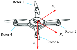
Figure 4: A quadcopter

As shown in Fig.4, a quadcopter’s dynamic model is expressed as[4]

$$\mathbf{\dot{p}} =\mathbf{v}$$

$$\mathbf{\dot{v}} =\mathbf{g-}\frac{1}{m}f\mathbf{R}\left(\mathbf{q}\right)\mathbf{e}_{3}$$

$$\mathbf{\dot{q}} =\left[\begin{array}[c]{cc}0&-\boldsymbol{\omega}^{\text{T}}\\ \boldsymbol{\omega}&-\left[\boldsymbol{\omega}\right]_{\times}\end{array}\right]\mathbf{q}$$ (20)

$$\mathbf{J}\boldsymbol{\dot{\omega}} =-\boldsymbol{\omega}\times\left(\mathbf{J}\boldsymbol{\omega}\right)+\mathbf{G}+\boldsymbol{\tau}$$ (21)

with

$$\left[\begin{array}[c]{c}f\\ \tau_{x}\\ \tau_{y}\\ \tau_{z}\end{array}\right]=\underset{\mathbf{H}}{\underbrace{\left[\begin{array}[c]{cccc}1&1&1&1\\ \frac{\sqrt{2}}{2}d&-\frac{\sqrt{2}}{2}d&\frac{\sqrt{2}}{2}d&-\frac{\sqrt{2}}{2}d\\ \frac{\sqrt{2}}{2}d&\frac{\sqrt{2}}{2}d&-\frac{\sqrt{2}}{2}d&-\frac{\sqrt{2}}{2}d\\ c_{M}\left/c_{T}\right.&-c_{M}\left/c_{T}\right.&c_{M}\left/c_{T}\right.&-c_{M}\left/c_{T}\right.\end{array}\right]}}\underset{\mathbf{T}}{\underbrace{\left[\begin{array}[c]{c}T_{1}\\ T_{2}\\ T_{3}\\ T_{4}\end{array}\right]}}$$ (22)

where $\mathbf{p}\in\mathbf{\mathbb{R}}^{3}$ and $\mathbf{v}\in\mathbf{\mathbb{R}}^{3}$ are position and velocity of the center of the multicopter in frame $o_{e}x_{e}y_{e}z_{e}$, respectively; the gravity vector is $\mathbf{g=[}0$ $0$ $g\mathbf{]}^{\text{T}}\in\mathbf{\mathbb{R}}^{3}$, the mass of the multicopter is $m>0;$ $\mathbf{R}\left(\mathbf{q}\right)\$is a rotation matrix, determined by a quaternion $\mathbf{q}\in\mathbf{\mathbb{R}}^{4}$; $\boldsymbol{\omega}\in\mathbf{\mathbb{R}}^{3}$ is the angular velocity of the multicopter expressed in frame $o_{b}x_{b}y_{b}z_{b};$ $\mathbf{J}\in\mathbf{\mathbb{R}}^{3\times 3}\$represents the multicopter moment of inertia; $\mathbf{G}$ represents the gyroscopic torque of rotors and propellers; $f$ $>0$ represents the magnitude of the total propeller thrust, $\boldsymbol{\tau=[}\tau_{x}$ $\tau_{y}$ $\tau_{z}\boldsymbol{]}^{\text{T}}\in\mathbf{\mathbb{R}}^{3}$ represents the moments generated by the propellers in the aircraft-body coordinate frame $o_{b}x_{b}y_{b}z_{b};$ $d$ $>0$ represents the distance between the body center and any motor; $c_{M},c_{T}>0$ are coefficients related to the pair of a propeller and motor; $T_{i}\in[0,T_{m}]$ are the propeller thrust with a maximum $T_{m}>0,$ $i=1,2,3,4.$ The objective is to design $T_{i}$ to make the multicopter track $\mathbf{p}_{d}\left(t\right)$ as accurately as possible in the case of both no failure and the first motor failing completely without loss of generality.

By using (4), we hope the desired total propeller thrust and desired rotation matrix to satisfy

$$\mathbf{g-}\frac{1}{m}f_{d}\mathbf{R}\left(\mathbf{q}_{d}\right)\mathbf{e}_{3}=\mathbf{a}_{d}$$

where $f_{d},\mathbf{q}_{d}$ are finally determined by the propeller thrust $T_{i}\in[0,T_{m}].$ Since

$$\mathbf{f}_{d}=-f_{d}\mathbf{R}\left(\mathbf{q}_{d}\right)\mathbf{e}_{3}$$ (23)

we can obtain that

$$\begin{array}[c]{ll}\underset{T_{id}\in\mathcal{C}\left(\left[0,T_{m}\right],\left[t_{0},t_{0}+T\right]\right),i=1,2,3,4}{\min}&\begin{array}[c]{l}w_{g}\left\|\int_{t_{0}}^{t_{0}+T}\left(\mathbf{f}_{g}\left(t\right)-m\mathbf{g}\right)\text{d}t\right\|^{2}+w_{t}\left\|\int_{t_{0}}^{t_{0}+T}\left(\mathbf{f}_{t}\left(t\right)-m\mathbf{a}_{d}\left(t\right)\right)\text{d}t\right\|^{2}\\ +w_{e}\int_{t_{0}}^{t_{0}+T}\left\|-\mathbf{f}_{g}\left(t\right)+\mathbf{f}_{t}\left(t\right)\right\|^{2}\text{d}t\end{array}\\ \text{s.t.}&\begin{array}[c]{lll}f_{d}\mathbf{R}\left(\mathbf{q}_{d}\right)\mathbf{e}_{3}&=&-\mathbf{f}_{g}+\mathbf{f}_{t}\\ \mathbf{\dot{q}}_{d}&=&\left[\begin{array}[c]{cc}0&-\boldsymbol{\omega}_{d}^{\text{T}}\\ \boldsymbol{\omega}_{d}&-\left[\boldsymbol{\omega}_{d}\right]_{\times}\end{array}\right]\mathbf{q}_{d}\\ \mathbf{J}\boldsymbol{\dot{\omega}}_{d}&=&-\boldsymbol{\omega}_{d}\times\left(\mathbf{J}\boldsymbol{\omega}_{d}\right)+\mathbf{G}+\boldsymbol{\tau}_{d}\\ \left[\begin{array}[c]{c}f_{d}\\ \boldsymbol{\tau}_{d}\end{array}\right]&=&\mathbf{HT}_{d},\mathbf{T}_{d}=[T_{1d}\text{ }T_{2d}\text{ }T_{3d}\text{ }T_{4d}]^{\text{T}}\end{array}.\end{array}$$ (24)

according to the gravity-compensation-first principle from the impulse viewpoint. Furthermore, if the first motor fails completely, then

$$\begin{array}[c]{ll}\underset{T_{i\text{d}}\in\mathcal{C}\left(\left[0,T_{m}\right],\left[t_{0},t_{0}+T\right]\right),i=2,3,4}{\min}&\begin{array}[c]{l}w_{g}\left\|\int_{t_{0}}^{t_{0}+T}\left(\mathbf{f}_{g}\left(t\right)-m\mathbf{g}\right)\text{d}t\right\|^{2}+w_{t}\left\|\int_{t_{0}}^{t_{0}+T}\left(\mathbf{f}_{t}\left(t\right)-m\mathbf{a}_{d}\left(t\right)\right)\text{d}t\right\|^{2}\\ +w_{e}\int_{t_{0}}^{t_{0}+T}\left\|-\mathbf{f}_{g}\left(t\right)+\mathbf{f}_{t}\left(t\right)\right\|^{2}\text{d}t\end{array}\\ \text{s.t.}&\begin{array}[c]{l}f_{d}\mathbf{R}\left(\mathbf{q}_{d}\right)\mathbf{e}_{3}=-\mathbf{f}_{g}+\mathbf{f}_{t}\\ \mathbf{\dot{q}}_{d}=\left[\begin{array}[c]{cc}0&-\boldsymbol{\omega}_{d}^{\text{T}}\\ \boldsymbol{\omega}_{d}&-\left[\boldsymbol{\omega}_{d}\right]_{\times}\end{array}\right]\mathbf{q}_{d}\\ \mathbf{J}\boldsymbol{\dot{\omega}}_{d}=-\boldsymbol{\omega}_{d}\times\left(\mathbf{J}\boldsymbol{\omega}_{d}\right)+\mathbf{G}_{a}+\boldsymbol{\tau}_{d}\\ \left[\begin{array}[c]{c}f_{d}\\ \boldsymbol{\tau}_{d}\end{array}\right]=\mathbf{HT}_{d},T_{1d}=0.\end{array}.\end{array}$$ (25)

III-C Application to a Fixed-Wing UAV Control

Figure 5: A fixed-wing UAV

As shown in Fig.5, a fixed-wing UAV’s dynamic model is expressed as [6]

$$\mathbf{\dot{p}} =\mathbf{v}$$

$$\mathbf{\dot{v}} =\mathbf{g-}\frac{1}{m}\mathbf{R}\left(\mathbf{q}\right)\left(\mathbf{f}_{p}+\mathbf{R}_{a}\left(\alpha,\beta\right)\mathbf{f}_{a}\right)$$ (26)

$$\mathbf{\dot{q}} =\left[\begin{array}[c]{cc}0&-\boldsymbol{\omega}^{\text{T}}\\ \boldsymbol{\omega}&-\left[\boldsymbol{\omega}\right]_{\times}\end{array}\right]\mathbf{q}$$ (29)

$$\mathbf{J}\boldsymbol{\dot{\omega}} =-\boldsymbol{\omega}\times\mathbf{J}\boldsymbol{\omega}+\mathbf{G}+\mathbf{m}_{p}+\mathbf{m}_{a}$$ (30)

where $\mathbf{f}_{p}\in\mathbf{\mathbb{R}}^{3}$ and $\mathbf{m}_{p}\in\mathbf{\mathbb{R}}^{3}$ are the force and torque produced by the propeller; $\mathbf{f}_{a},\mathbf{m}_{a}$ are the force and torque produced by the aerodynamic force; the other physical meaning is the same to those in (21) because both a quadcopter and a fixed-wing UAV are rigid body. Let $\mathbf{v}_{w}\in\mathbf{\mathbb{R}}^{3}$ be wind velocity. Define the airspeed $\mathbf{v}_{a}\in\mathbf{\mathbb{R}}^{3}$ as

$$\mathbf{v}_{a}=\mathbf{R}^{\text{T}}\left(\mathbf{v-v}_{w}\right).$$

The airspeed is $V_{a}=\left\|\mathbf{v}_{a}\right\|$, angle of attack $\alpha$ and sideslip angle $\beta$ are

$$\alpha =\tan^{-1}\left(\frac{\mathbf{v}_{a,3}}{\mathbf{v}_{a,1}}\right)$$

$$\beta =\sin^{-1}\left(\frac{\mathbf{v}_{a,2}}{\left\|\mathbf{v}_{a}\right\|}\right)$$

where $\mathbf{x}_{i}$ is the $i$th element of $\mathbf{x.}$ Let $\mathbf{v}_{e}\in\mathbf{\mathbb{R}}^{3}$ be the downwash velocity of the propeller as shown in Fig.6, defined as

$$\mathbf{v}_{e}=\left[\begin{array}[c]{c}V_{e}\\ 0\\ 0\end{array}\right]$$

where $V_{e}=k_{m}\delta_{t}$ is the speed of the air as it leaves the propeller, $k_{m}>0$ and $\delta_{t}\in\left[0,1\right]$ is the pluse-width-modulation command.

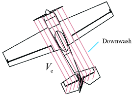
Figure 6: Downwash

For simplicity, as shown in Fig.6, we assume that the elevator, rudder are affected fully by the downwash [7]. Aerodynamic force consists of the lift, drag and side force. The lift is perpendicular to the airspeed while the drag is in line with and opposing the airspeed. The directions of drag, side force, and lift form a right-handed frame. Similar to book [5], we have

$$\mathbf{f}_{p} =\frac{1}{2}\rho S_{p}C_{p}\left[\begin{array}[c]{c}V_{e}^{2}-V_{a}^{2}\\ 0\\ 0\end{array}\right]$$

$$\mathbf{m}_{p} =\left[\begin{array}[c]{c}-k_{T_{p}}\left(k_{\Omega}\delta_{t}\right)^{2}\\ 0\\ 0\end{array}\right]$$

$$\mathbf{f}_{a}=\left[\begin{array}[c]{c}-\frac{1}{2}\rho V_{a}^{2}SC_{Df}\left(\alpha,q\right)-\frac{1}{2}\rho V_{a}^{2}SC_{Dw_{l}}\left(\alpha,q,\delta_{al}\right)-\frac{1}{2}\rho V_{a}^{2}SC_{Dw_{r}}\left(\alpha,q,\delta_{ar}\right)-\frac{1}{2}\rho V_{e}^{2}SC_{D_{e}}\left(\delta_{e}\right)\\ \frac{1}{2}\rho V_{a}^{2}SbC_{lf}\left(\beta,p,r\right)+\frac{1}{2}\rho V_{a}^{2}SbC_{lw_{l}}\left(\beta,p,r,\delta_{al}\right)+\frac{1}{2}\rho V_{a}^{2}SbC_{lw_{r}}\left(\beta,p,r,\delta_{ar}\right)+\frac{1}{2}\rho V_{e}^{2}SbC_{l_{r}}\left(\delta_{r}\right)\\ \frac{1}{2}\rho V_{a}^{2}SC_{Lf}\left(\alpha,q\right)+\frac{1}{2}\rho V_{a}^{2}SC_{Lw_{l}}\left(\alpha,q,\delta_{al}\right)+\frac{1}{2}\rho V_{a}^{2}SC_{Lw_{r}}\left(\alpha,q,\delta_{ar}\right)+\frac{1}{2}\rho V_{e}^{2}SC_{Le}\left(\delta_{e}\right)\end{array}\right]$$

$$\mathbf{m}_{a}=\left[\begin{array}[c]{c}l\\ m\\ n\end{array}\right]=\left[\begin{array}[c]{c}\frac{1}{2}\rho V_{a}^{2}SbC_{lf}\left(\beta,p,r\right)+\frac{1}{2}\rho V_{a}^{2}SbC_{lw_{l}}\left(\beta,p,r,\delta_{al}\right)\\ \text{ \ \ \ \ \ \ \ \ \ }+\frac{1}{2}\rho V_{a}^{2}SbC_{lw_{r}}\left(\beta,p,r,\delta_{ar}\right)+\frac{1}{2}\rho V_{e}^{2}SbC_{l_{r}}\left(\delta_{r}\right)\\ \frac{1}{2}\rho V_{a}^{2}ScC_{mf}\left(\alpha,q\right)+\frac{1}{2}\rho V_{a}^{2}ScC_{mw_{l}}\left(\alpha,q,\delta_{al}\right)\\ \text{ \ \ \ \ \ \ \ \ \ }+\frac{1}{2}\rho V_{a}^{2}ScC_{mw_{r}}\left(\alpha,q,\delta_{ar}\right)+\frac{1}{2}\rho V_{w}^{2}ScC_{m_{e}}\left(\delta_{e}\right)\\ \frac{1}{2}\rho V_{a}^{2}SbC_{nf}\left(\beta,p,r\right)+\frac{1}{2}\rho V_{a}^{2}SbC_{nw_{l}}\left(\beta,p,r,\delta_{al}\right)\\ \text{ \ \ \ \ \ \ \ \ \ }+\frac{1}{2}\rho V_{a}^{2}SbC_{nw_{r}}\left(\beta,p,r,\delta_{ar}\right)+\frac{1}{2}\rho V_{w}^{2}SbC_{n_{r}}\left(\delta_{r}\right)\end{array}\right]$$

where $\rho$ is the air density, $S$ is the wing area, $b$ is the wingspan, $c$ is the mean chord of the wing, $S_{p}$ is the area swept out by the propeller, $k_{\Omega}\delta_{t}$ is the propeller speed and $k_{T_{p}}$ is a constant determined by experiment, $C_{p}$ is a constant determined by experiment; the aerodynamic force and moments are produced by the left wing including its aileron, the right wing including its aileron, the fuselage, elevator and rudder; the left and right aileron angles are denoted by $\delta_{al},\delta_{ar}\in[-\delta_{am,}\delta_{am,}]$, elevator angle by $\delta_{e}\in[-\delta_{em,}\delta_{em,}]$ and rudder angle by $\delta_{r}\in[-\delta_{rm,}\delta_{rm,}].$ Furthermore, the aerodynamic force and moments are produced by both the airflow and downwash, where the physical meaning of components is shown in Tables 1-2. Due to the symmetry of the left and right ailerons, we have

$$C_{Dw_{l}}\left(\alpha,q,\cdot\right) =-C_{Dw_{r}}\left(\alpha,q,\cdot\right)$$

$$C_{lw_{l}}\left(\beta,p,r,\cdot\right) =-C_{lw_{r}}\left(\beta,p,r,\cdot\right)$$

$$C_{Lw_{l}}\left(\alpha,q,\cdot\right) =-C_{Lw_{r}}\left(\alpha,q,\cdot\right)$$

$$C_{lw_{l}}\left(\beta,p,r,\cdot\right) =-C_{lw_{r}}\left(\beta,p,r,\cdot\right)$$

$$C_{mw_{l}}\left(\alpha,q,\cdot\right) =-C_{mw_{r}}\left(\alpha,q,\cdot\right)$$

$$C_{nw_{l}}\left(\beta,p,r,\cdot\right) =-C_{nw_{r}}\left(\beta,p,r,\cdot\right).$$

Table 1. Aerodynamic force components

Symbol Meaning

$$-\frac{1}{2}\rho V_{a}^{2}SC_{Df}\left(\alpha,q\right)$$ Drag by the fuselage

Drag by the left wing including its aileron

Drag by the right wing including its aileron

Drag by the rudder caused by downwash

Side force by the fuselage

Side force by the left wing including its aileron

Side force by the right wing including its aileron

Side force by the rudder caused by downwash

Lift by the fuselage

Lift by the left wing including its aileron

Lift by the right wing including its aileron

Lift by the rudder caused by downwash

Table 2. Aerodynamic moment components

Symbol Meaning

$$\frac{1}{2}\rho V_{a}^{2}SbC_{lf}\left(\beta,p,r\right)$$ Roll moment by the fuselage

Roll moment by the left wing including its aileron

Roll moment by the right wing including its aileron

Roll moment by the rudder caused by downwash

Pitch moment by the fuselage

Pitch moment by the left wing including its aileron

Pitch moment by the right wing including its aileron

Pitch moment by the elevator

Yaw moment by the fuselage

Yaw moment by the left wing including its aileron

Yaw moment by the right wing including its aileron

Yaw moment by the rudder caused by downwash

    

The objective is to design $\delta_{t},\delta_{al},\delta_{ar},\delta_{e},\delta_{r}$ to replicate the accident shown in Fig.1. First, make the UAV track $\mathbf{p}_{d}\left(t\right)$ as accurately as possible when no failure happens. Then, make it land safely when the left half of the wings loses completely. By using (4), we hope the desired total propeller thrust and desired rotation matrix satisfy

$$\mathbf{g-}\frac{1}{m}\mathbf{R}\left(\mathbf{q}_{d}\right)\left(\mathbf{f}_{pd}+\mathbf{R}_{a}\left(\alpha_{d},\beta_{d}\right)\mathbf{f}_{ad}\right)=\mathbf{a}_{d}$$

where $\mathbf{f}_{pd},\mathbf{q}_{d},\alpha_{d},\beta_{d},\mathbf{f}_{ad}$ are finally determined by $\delta_{t},\delta_{al},\delta_{ar},\delta_{e},\delta_{r}.$ If the left half of wings loses completely, then $\delta_{al}=0$ and $C_{\cdot w_{l}}=0.$ Since

$$\mathbf{f}_{d}=\mathbf{-}\frac{1}{m}\mathbf{R}\left(\mathbf{q}_{d}\right)\left(\mathbf{f}_{pd}+\mathbf{R}_{a}\left(\alpha_{d},\beta_{d}\right)\mathbf{f}_{ad}\right)$$ (31)

we can obtain that

$$\begin{array}[c]{ll}\underset{}{\underset{\delta_{ed}\in[-\delta_{em,}\delta_{em,}],\delta_{rd}\in[-\delta_{rm,}\delta_{rm,}]}{\underset{\delta_{td}\in\left[0,1\right],\delta_{ald},\delta_{ard}\in[-\delta_{am,}\delta_{am,}],}{\min}}}&\begin{array}[c]{l}w_{g}\left\|\int_{t_{0}}^{t_{0}+T}\left(\mathbf{f}_{g}\left(t\right)-m\mathbf{g}\right)\text{d}t\right\|^{2}+w_{t}\left\|\int_{t_{0}}^{t_{0}+T}\left(\mathbf{f}_{t}\left(t\right)-m\mathbf{a}_{d}\left(t\right)\right)\text{d}t\right\|^{2}\\ +w_{e}\int_{t_{0}}^{t_{0}+T}\left\|-\mathbf{f}_{g}\left(t\right)+\mathbf{f}_{t}\left(t\right)\right\|^{2}\text{d}t\end{array}\\ \text{s.t.}&\begin{array}[c]{l}\mathbf{-}\frac{1}{m}\mathbf{R}\left(\mathbf{q}_{d}\right)\left(\mathbf{f}_{pd}\left(\delta_{td}\right)+\mathbf{R}_{a}\left(\alpha_{d},\beta_{d}\right)\mathbf{f}_{ad}\left(\delta_{td},\delta_{ald},\delta_{ard},\delta_{ed},\delta_{rd}\right)\right)\\ =-\mathbf{f}_{g}+\mathbf{f}_{t}\\ \mathbf{\dot{q}}_{d}=\left[\begin{array}[c]{cc}0&-\boldsymbol{\omega}_{d}^{\text{T}}\\ \boldsymbol{\omega}_{d}&-\left[\boldsymbol{\omega}_{d}\right]_{\times}\end{array}\right]\mathbf{q}_{d}\\ \mathbf{J}\boldsymbol{\dot{\omega}}_{d}=-\boldsymbol{\omega}_{d}\times\mathbf{J}\boldsymbol{\omega}_{d}+\mathbf{G}+\mathbf{m}_{p}\left(\delta_{td}\right)+\mathbf{m}_{a}\left(\delta_{td},\delta_{ald},\delta_{ard},\delta_{ed},\delta_{rd}\right)\end{array}\end{array}$$ (32)

according to the gravity-compensation-first principle from the impulse viewpoint. Furthermore, if the left half of wings loses completely, then

$$\begin{array}[c]{ll}\underset{\delta_{ed}\in[-\delta_{em,}\delta_{em,}],\delta_{rd}\in[-\delta_{rm,}\delta_{rm,}]}{\underset{\delta_{td}\in\left[0,1\right],\delta_{ard}\in[-\delta_{am,}\delta_{am,}],}{\min}}&\begin{array}[c]{l}w_{g}\left\|\int_{t_{0}}^{t_{0}+T}\left(\mathbf{f}_{g}\left(t\right)-m\mathbf{g}\right)\text{d}t\right\|^{2}+w_{t}\left\|\int_{t_{0}}^{t_{0}+T}\left(\mathbf{f}_{t}\left(t\right)-m\mathbf{a}_{d}\left(t\right)\right)\text{d}t\right\|^{2}\\ +w_{e}\int_{t_{0}}^{t_{0}+T}\left\|-\mathbf{f}_{g}\left(t\right)+\mathbf{f}_{t}\left(t\right)\right\|^{2}\text{d}t\end{array}\\ \text{s.t.}&\begin{array}[c]{l}\mathbf{-}\frac{1}{m}\mathbf{R}\left(\mathbf{q}_{d}\right)\left(\mathbf{f}_{pd}\left(\delta_{td}\right)+\mathbf{R}_{a}\left(\alpha_{d},\beta_{d}\right)\mathbf{f}_{ad}\left(\delta_{td},\delta_{ald},\delta_{ard},\delta_{ed},\delta_{rd}\right)\right)\\ =-\mathbf{f}_{g}+\mathbf{f}_{t}\\ \mathbf{\dot{q}}_{d}=\left[\begin{array}[c]{cc}0&-\boldsymbol{\omega}_{d}^{\text{T}}\\ \boldsymbol{\omega}_{d}&-\left[\boldsymbol{\omega}_{d}\right]_{\times}\end{array}\right]\mathbf{q}_{d}\\ \mathbf{J}\boldsymbol{\dot{\omega}}_{d}=-\boldsymbol{\omega}_{d}\times\left(\mathbf{J}\boldsymbol{\omega}_{d}\right)+\mathbf{G}+\mathbf{m}_{p}\left(\delta_{td}\right)+\mathbf{m}_{a}\left(\delta_{td},\delta_{ald},\delta_{ard},\delta_{ed},\delta_{rd}\right)\\ \delta_{ald}=0,\text{ }C_{\cdot w_{l}}=0.\end{array}.\end{array}$$ (33)

IV CONCLUSIONS

According to the first principle, the gravity-compensation-first principle is developed. It states that all control gives priority to compensating for the effect caused by the gravity of the aircraft, with the left authority used to meet the requirements of the desired motion of the aircraft. According to Newton’s second law, the principle is further formulated as optimization problems in three aspects: force, impulse, and energy based on a mass point model. Furthermore, the principle is applied to a quadcopter and a fixed-wing UAV with severe failure. Model predictive control methods can help solve the problems by the gravity-compensation-first principle.

References

- [1] Xiang Yu, Jin Jiang. A survey of fault-tolerant controllers based on safety-related issues. Annual Reviews in Control, 39, 2015, 46-57.
- [2] M Steinberg. Historical overview of research in reconfigurable flight control. Proceedings of the Institution of Mechanical Engineers Part G Journal of Aerospace Engineering, 2015, 219(4): 263-275.
- [3] Saša V. Raković, William S. Levine. Handbook of Model Predictive Control. Birkhäuser Basel, 2018.
- [4] Quan Quan. Introduction to Multicopter Design and Control. Springer, Singapore, 2017.
- [5] Randal W. Beard and Timothy W. McLain. Small Unmanned Aircraft: Theory and Practice. Princeton University Press, 2012.
- [6] Jinni Zhou, Ximin Lyu, Zexiang Li, Shaojie Shen, Fu Zhang. A unified control method for quadrotor tail-sitter UAVs in all flight modes: Hover, transition, and level flight. 2017 IEEE/RSJ International Conference on Intelligent Robots and Systems (IROS), Vancouver, BC, Canada, 24-28 Sept. 2017.
- [7] Takaaki Matsumoto, Koichi Kita, Ren Suzuki, Atsushi Oosedo, Kenta Go, Yuta Hoshino, Atsushi Konno, Masaru Uchiyama. A hovering control strategy for a tail-sitter VTOL UAV that increases stability against large disturbance. 2010 IEEE International Conference on Robotics and Automation, Anchorage, AK, USA, 3-7 May 2010.