Blind Face Restoration: Benchmark Datasets and a Baseline Model

Abstract

Blind Face Restoration (BFR) aims to construct a high-quality (HQ) face image from its corresponding low-quality (LQ) input. Recently, many BFR methods have been proposed and they have achieved remarkable success. However, these methods are trained or evaluated on privately synthesized datasets, which makes it infeasible for the subsequent approaches to fairly compare with them. To address this problem, we first synthesize two blind face restoration benchmark datasets called EDFace-Celeb-1M (BFR128) and EDFace-Celeb-150K (BFR512). State-of-the-art methods are benchmarked on them under five settings including blur, noise, low resolution, JPEG compression artifacts, and the combination of them(full degradation). To make the comparison more comprehensive, five widely-used quantitative metrics and two task-driven metrics including Average Face Landmark Distance (AFLD) and Average Face ID Cosine Similarity (AFICS) are applied. Furthermore, we develop an effective baseline model called Swin Transformer U-Net (STUNet). The STUNet with U-net architecture applies an attention mechanism and a shifted windowing scheme to capture long-range pixel interactions and focus more on significant features while still being trained efficiently. Experimental results show that the proposed baseline method performs favourably against the SOTA methods on various BFR tasks. The codes, datasets, and trained models are publicly available at: https://github.com/bitzpy/Blind-Face-Restoration-Benchmark-Datasets-and-a-Baseline-Model.

1 Introduction

Face images are very important in both academic research areas and commercial applications, as they contain rich and unique identity information. However, in real-world scenarios, face images usually involve complex degradations such as blur, noise, low resolution, compression artifacts, or the combination of them. Face restoration aims at generating a realistic and faithful face image from a degraded one, which can be used for face detection, face recognition, and many other vision tasks. Due to its significant research value and wide range of application scenarios, face restoration has been attracting more and more attention in the image processing and computer vision communities[1, 2, 3].

For face restoration, traditional methods typically focus on a single type of degradation. Thus face restoration is divided into numerous sub-tasks, including deblurring [1], denoising [4, 5], super-resolution [6, 7, 8, 9, 10], compression artifact removal [11]. Yet real-world face images are often degraded owing to more than one factor. It is a matter of course that these methods designed for one specific and known degradation perform with limited generalization in the scenery of real-world face images. As such, Blind Face Restoration (BFR) which recovers high-quality (HQ) face images from low-quality (LQ) inputs with unknown degradations is more practical and thus attracts increasing attention in recent years.

Although the existing BFR methods have demonstrated excellent and remarkable abilities to generate realistic and faithful images in recent years, there are still problems unsolved in the community which hinder the progress of the BFR task. First, most of the current BFR methods are trained or evaluated on private facial datasets. This leads to unnecessary and expensive retraining costs. When a new BFR algorithm is proposed, for a fair comparison, authors have to synthesize datasets by themselves and retrain all previous methods instead of reporting their previous results directly. Second, the scale of the private datasets used by the existing methods is usually small. This raises an doubt about the generalization of the methods trained with them. To advance the development of BFR, we synthesize two benchmark datasets called EDFace-Celeb-1M (BFR128) and EDFace-Celeb-150K (BFR512) based on the EDFace-Celeb dataset [12]. EDFace-Celeb-1M (BFR128) contains about $1.5$ million images of resolution $128\times 128$, of which $1.36$ million images are used for training and $145$ thousand images are used for testing. EDFace-Celeb-150K (BFR512) includes about $149$K images with a resolution of $512\times 512$. The number of training images is about $132$K and the number of testing is about $17$K. Several sample images from them are shown in Fig. 1.

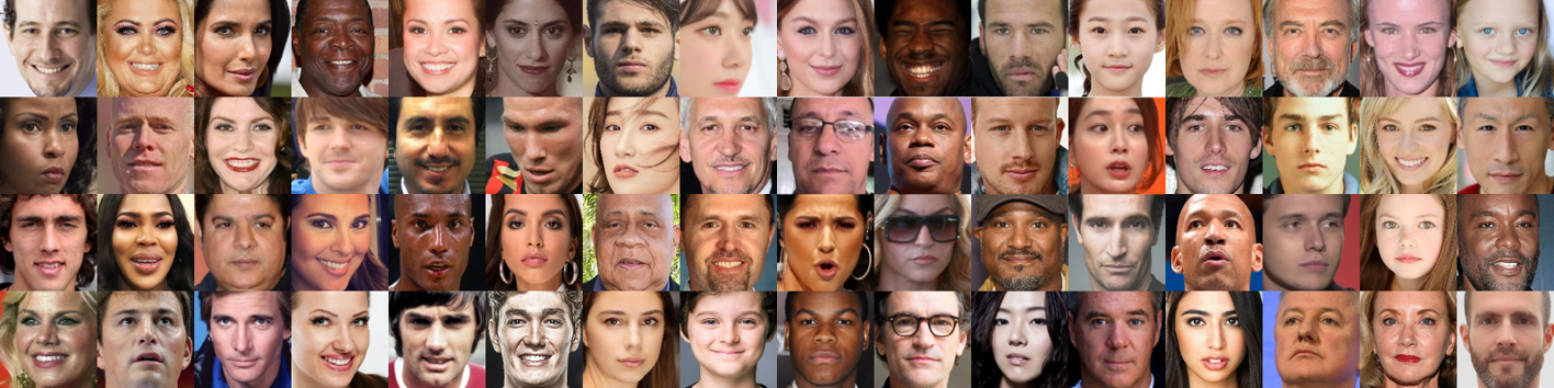
(a) Sample face images from the EDFace-Celeb-1M (BFR128) dataset

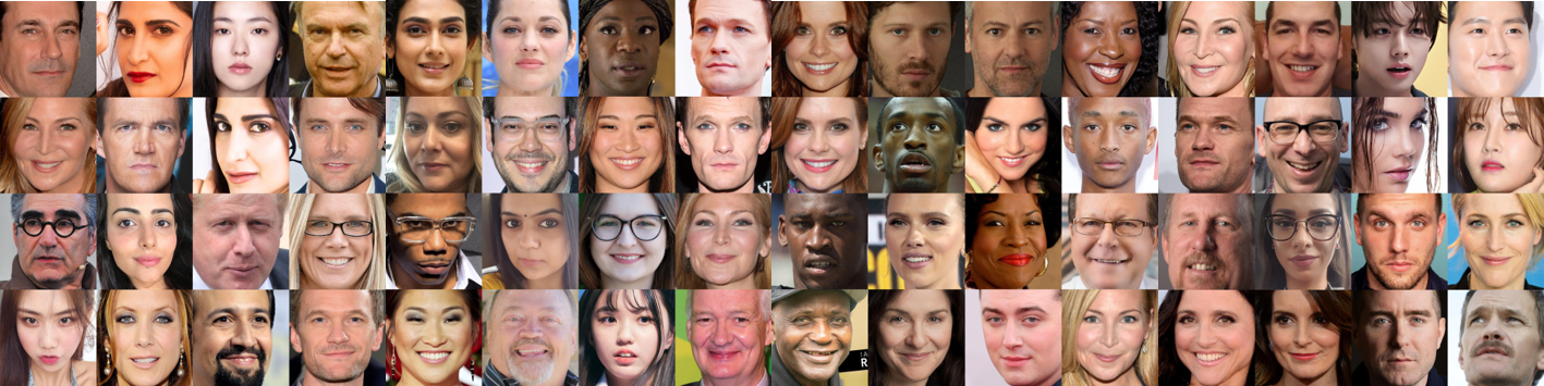
(b) Sample face images from the EDFace-Celeb-150K (BFR512) dataset

Figure 1: Sample images from the synthesized datasets. The two datasets contain a large number of face images. We show representative images from subjects of different genders, ages and races.

We present five degradation settings for each of the two datasets to benchmark current representative BFR methods. These settings include blur, noise, low resolution, JPEG compression artifacts, and the combination of them. By evaluating state-of-the-art BFR methods on the two datasets under the above five settings, we gain a more comprehensive understanding of existing BFR methods. Additionally, considering that blind face restoration can be used in many down-stream vision tasks such as face detection and face recognition, we introduce two task-driven metrics, i.e., Average Face Landmark Distance (AFLD) and Average Face ID Cosine Similarity(AFICS), to assess the performance of these methods more objectively and exhaustively.

Finally, we propose a novel Swin Transformer U-Net(STUNet) for the BFR task. Compared with traditional CNN-based models, our STUNet introduces an attention mechanism to enhance the feature representation ability by capturing global interactions between pixels. For most Transformer-based models, the expensive training overhead hinders their usefulness. To this end, we utilize the shifted windowing scheme [13] which limits the self-attention computation in a fixed-size local window and meanwhile achieves the cross-window connection.

Overall, the contributions of our work are four-fold:

• Firstly, we synthesize two large-scale benchmark datasets for BFR. These two datasets include millions of facial images covering all the typical degradation settings as well as a combination of them. On top of our datasets, it is convenient for future research to evaluate the proposed methods and fair to compare with existing methods.

• Secondly, we evaluate several representative state-of-the-art BFR methods on two datasets, employing five popularly used quantitative metrics. With such extensive evaluation, we have a clearer understanding of the advantages and disadvantages of the SOTA methods.

• Thirdly, we additionally design two task-driven metrics, AFLD and AFICS, to evaluate the performance of the state-of-the-art BFR methods. This study provides a new perspective to investigate the BFR methods in terms of their influence on down-stream tasks like face detection and recognition.

• Fourthly, we propose a baseline model STUNet which adopts the strong Transformer architecture and is capable of enhancing feature representation. Extensive experiments illustrate its superiority on the BFR task.

2 Related Work

2.1 Face Restoration Datasets

Currently, there are no publicly available datasets specifically for blind face restoration. Most of the face restoration methods use existing face datasets including FFHQ [14], CASIA-WebFace [15], VGGFace2 [16], IMDB-WIKI [17], CelebA [18], Helen [19], LWF [20], BioID [21], AFLW [22], and generate low quality images according to their demands. In 2001, BioID dataset [21] is presented and it contains $1,521$ images of $23$ subjects. Huang et al. [20] introduce the labeled faces in the wild (LFW) dataset which includes $13,233$ images of $5,749$ subjects. The Annotated Facial Landmarks in the Wild (AFLW) [22] dataset is created, including $25,993$ images annotated with up to $21$ landmarks per image. The Helen dataset consists of $2,330$ high-resolution, accurately labeled face images. The CASIA-WebFace dataset [15] is presented in 2014 and it includes $494,414$ images. Liu et al. [18] introduce the CelebA dataset including $200$K images by labeling images selected from CelebFaces [23] and Rothe et al. [17] propose the IMDB-WIKI dataset containing $523,051$ face images. More recently, Cao et al. [16] introduce the VGGFace2 dataset which has $3.31$ million images from a large number of subjects. Karras et al. [14] release the FFHQ dataset. It contains $70$K highly varied and high-quality images. See Table I for a clear overview of these datasets.

TABLE I: Representative face datasets used in face restoration tasks. Specifically for training and evaluating BFR methods, these popularly-used face datasets do not provide public pairs of LQ and HQ images. In the table, ”$-$” means that the resolution of the images in the dataset is not fixed.

Dataset	Size	Resolution	HQ-LQ
BioID[21]	1521	$384\times 288$	$\times$
LFW[20]	13,233	$250\times 250$	$\times$
AFLW[22]	25,993	$-$	$\times$
Helen[19]	2330	$-$	$\times$
CASIA-WebFace[15]	494,414	$250\times 250$	$\times$
CelebA[18]	200,000	$-$	$\times$
IMDB-WIKI[17]	524,230	$-$	$\times$
VGGFace2[16]	3,310,000	$-$	$\times$
FFHQ[14]	70,000	$1024\times 1024$	$\times$
EDFace-Celeb-1M(BFR128)	1,505,888	$128\times 128$	$\checkmark$
EDFace-Celeb-150K(BFR512)	148,962	$512\times 512$	$\checkmark$

2.2 Face Restoration Methods

With the development of deep learning, image restoration has witnessed great success on many tasks, such as image deblurring [24, 25, 26, 27], image denoising [28, 29, 4, 5], image super-resolution [6, 8, 30, 31, 32, 9, 33], image compression artifact removal [34, 11]. Face restoration, as an important and popular branch of image restoration, also shows outstanding performance in generating clear and faithful face images in recent years. Thanks to the special facial structure of the face image, there are numerous well-designed algorithms for face restoration. Among these methods, traditional face restoration methods [35, 7, 1, 36, 37, 38, 12, 39, 40, 11, 9] pre-define the degradation type before training, thus leading to poor generalization ability. Considering the fact that we cannot know the degradation type when a real-world image is degraded, researchers pay more attention to the so-called blind face restoration (BFR) problem [41, 42, 43, 44, 45, 46], which is more challenging due to the unknown degradations.

Cao et al.[35] utilize deep reinforcement learning to sequentially discover attended patches so that high-resolution (HR) faces can be recovered by fully exploiting the global interdependency of the face images. Chen et al.[7] performer face super-resolution with facial geometry prior. Shen et al. [1] present a deep convolutional neural network and take the advantage of semantic information to solve the face deblurring problem. Kim et al. [36] propose a face super-resolution method that applies a novel facial attention loss to focus on restoring facial attributes. Menon et al. [37] propose PULSE, which traverses the high-resolution natural image manifold, searching for images that downscale to the original LR image. When it comes to BFR, Li et al. [41] design a GFRNet including both a wrapping sub-network and a reconstruction sub-network, with a guided image as input for BFR. Moreover, they extend their work by using multi-scale component dictionaries instead of a single reference [42]. HiFaceGAN, a collaborative suppression and replenishment approach, is introduced by Yang et al. [43] to progressively replenish facial details. Yang et al. [44] propose a GAN prior embedded network to generate visually photo-realistic images. Chen et al. [45] learn facial semantic prior and make use of multi-scale inputs to recover high-quality images. Wang et al. [46] leverage pre-trained face GAN to provide diverse and rich priors, solving the contradiction between inaccurate priors offered by low-quality inputs and inaccessible high-quality references.

2.3 Vision Transformer

Natural language processing (NLP) model Transformer [47] proposed by Vaswani et al. performs favorably against state-of-the-art methods in many NLP tasks. Due to its outstanding ability in feature extraction, Transformer has won great popularity in the computer vision community. A lot of well-designed attention architectures [48, 49, 50, 51, 52, 53, 54, 55, 56] have been proposed for computer vision tasks, advancing the development of vision transformer. However, many of these architectures are not easy to be implemented effectively on hardware accelerators. Dosovitskiy et al. [57] introduce Vision Transformer (ViT), which shows more excellent speed-accuracy trade-off on the image classification task than traditional CNN models. To address the limitation that the ViT needs to be trained on large-scale datasets (i.e., JFT-300M) to achieve its best performance, DeiT et al. [58] propose useful training strategies so that ViT can also be well trained on the smaller ImageNet-1K dataset. Although the result of ViT has been successful, ViT still suffers from the difficulty that the training speed of high-resolution images is unbearably slow for the quadratic increase in complexity with image size. Swin Transformer [13] presented by Liu et al. whose self-attention is computed with shifted window scheme, greatly improves the training efficiency. Besides, Swin Transformer serving as a general-purpose backbone has become the state-of-the-art method in many vision tasks. Due to the impressive performance of Transformer, there are also several Transformer-based methods [59, 60, 61, 62] for image restoration. Chen et al. [60] propose an image processing transformer (IPT) which is a pre-trained model and can be employed on intended restoration tasks such as image denoising and image super-resolution after fine-tuning. Cao et al. [59] propose VSR-Transformer that utilizes a self-attention mechanism to restore high-resolution videos from low-resolution inputs. Wang et al. [61] present a Uformer using window-based self-attention rather than global self-attention for image restoration. Liang et al. [62] introduce a strong baseline model called SwinIR for image restoration, which is based on the Swin Transformer [13].

(a) HQ

(b) Blur

(c) Noise

(d) JPEG

(e) Low Resolution

(f) Full

Figure 2: Exemplar images showing the five degradation settings, including blur, noise, JPEG compression, low resolution, and the combination of them (Full), along with the original HQ image.

3 Benchmark Datasets

We aim to provide a comprehensive study by quantitatively evaluating the recent state-of-the-art blind face restoration methods. To this end, we need to synthesize appropriate datasets which have not only high-quality images but also their corresponding low-quality images. In this section, we first introduce the construction of the synthesized datasets. And then, we introduce the degradation settings of the two datasets used for both training and evaluation.

3.1 The Synthesized Datasets

In both EDFace-Celeb-1M (BFR128) & EDFace-Celeb-150K (BFR512), we provide high-quality images and for each high-quality image we generate several types of degraded low-quality images. The high-quality images are derived from the EDFace-Celeb [12] dataset. The EDFace-Celeb is a million-scale face image dataset that contains images from more than $20$K different subjects. These subjects are from different races and in different age groups. Each subject has $100\sim 1000$ face images from the Internet. We select about $1.5$M images whose resolution is $128\times 128$ from EDFace-Celeb-1M to synthesize the EDFace-Celeb-1M (BFR128) dataset. Similarly, we construct the EDFace-Celeb-150K (BFR512) dataset by choosing about $150$K images with a resolution is $512\times 512$ from EDFace-Celeb-150K. Then we fix the division of training and testing samples in the two datasets. Besides, we synthesize five settings containing pairs of LQ and HQ face images for training and evaluating face restoration methods, which are detailed in the following section.

3.2 Image Degradation Settings

To simulate the complex real-world image low-quality factors, we degrade the quality of HQ images with various types of degradation operations. Following the degradation strategy [43], we employ five degradation settings, called Blur, Noise, JPEG, LR, and Full. Each setting consists of corresponding HQ and LQ image pairs. To obtain the Blur setting, we convolve HQ images with a Gaussian or Motion blur kernel. The images in the Noise setting are generated by adding one of Gaussian, Laplace, and Poisson noise to the HQ images. Compressing HQ images by JPEG, the JPEG setting is created. For the LR setting, we use Bicubic interpolation with a random downsampling factor between 2 and 8 to synthesize low-resolution images. Besides, the Full setting images are synthesized by randomly superimposing the above four types of degradations over HQ images. These settings correspond to the face deblurring, denoising, JPEG compression artifact removal, super-resolution, and blind restoration tasks. Our synthetic datasets are sufficiently challenging so as to fulfill the goal of training BFR approaches in the real-world scenery. Fig. 2 shows exemplar images of an original HQ image and its LQ counterparts by different degradation operations.

4 STUNet

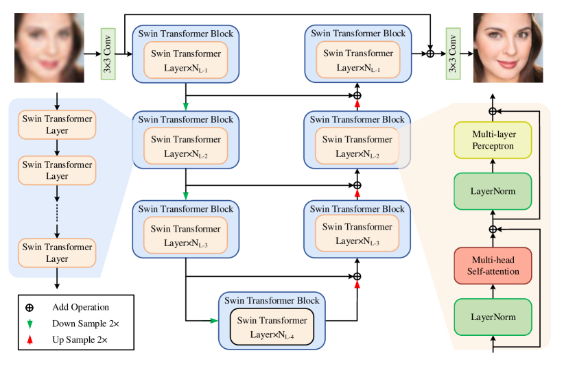
Figure 3: The architecture of the proposed STUNet for blind face restoration. STUNet takes a low-quality image as input, then uses a convolutional layer to extract shallow features. Next, we use several Swin Transformer blocks to extract deep features further. Finally, a convolutional layer is used to recover a high-quality face image from the deep features.

Blind face restoration is a challenging task because of its complex degradation of input images. Existing BFR methods are typically based on a convolutional neural network. While currently Swin Transformer [13] based methods have been achieving state-of-the-art performance in many computer vision tasks. We thus propose a novel baseline model for blind face restoration, which uses Swin Transformer as the backbone instead of a convolutional neural network. We aim to design a lightweight but promising network architecture that can be conveniently used and benefit future research. In the following, we introduce our proposed baseline model Swin Transformer U-net (STUNet).

4.1 Network Architecture

As shown in Fig. 3, the proposed STUNet consists of three parts: preprocessing embedding module, feature extraction module, and image restoring module.

Preprocessing Embedding Module. Given a low-quality input image $I_{LQ}{\in}\mathbb{R}^{H{\times}W{\times}C_{I}}$ ($H$ is the image height, $W$ is the image width, and $C_{I}$ is the image channel number), our STUNet first applies a $3\times 3$ convolutional layer to extract a shallow feature embedding as

$$F_{C0}=H_{C0}(I_{LQ}),$$ (1)

where $F_{C0}{\in}\mathbb{R}^{H{\times}W{\times}C}$ is the features extracted via the $3\times 3$ convolutional layer, $C$ is the channel number of the feature, and $H_{C0}$ denotes the function representing the first convolutional layer. The convolutional layer works well in mapping low dimensional image space to high dimensional feature space in a simple yet effective way.

Feature Extraction Module. The low-level features from the preprocessing embedding module are then processed by a feature extraction module to obtain deep features. The feature extraction module is a symmetric 4-level encoder-decoder architecture composed of Swin Transformer blocks (STB) at different levels. In the encoder part, the shallow feature $F_{C0}$ is first fed to a Swin Transformer block to extract features $F_{e1}{\in}\mathbb{R}^{H{\times}W{\times}C}$ by

$$F_{e1}=H_{e1}(F_{C0}),$$ (2)

where $H_{e1}$ is the function to represent the process by the Swin Transformer block at the first level. Next, we apply the pixel-unshuffle operation to downsample the feature $F_{e1}$, and then we obtain deeper features $F_{e2}{\in}\mathbb{R}^{\frac{H}{2}{\times}\frac{W}{2}{\times}2C}$ via a Swin Transformer block as

$$F_{e2}=H_{e2}(H_{down}(F_{e1})),$$ (3)

where $H_{down}$ and $H_{e2}$ denote the downsampling function and the process by the Swin Transformer block at the second level.

Similarly, the encoder further extracts the latent features $F_{e3}{\in}\mathbb{R}^{\frac{H}{4}{\times}\frac{W}{4}{\times}4C}$ and $F_{e4}{\in}\mathbb{R}^{\frac{H}{8}{\times}\frac{W}{8}{\times}8C}$ as the following,

$$F_{e3}=H_{e3}(H_{down}(F_{e2})),$$ (4)

$$F_{e4}=H_{e4}(H_{down}(F_{e3})),$$ (5)

where $H_{e3}$, $H_{e4}$ are the functions representing Swin Transformer block at level-3 and level-4, respectively.

From the top to bottom level, the encoder converts the high-resolution shallow features with a small number of channels to the low-resolution latent feature with a large number of channels. Next, the decoder progressively reconstructs the high-resolution features from the low-resolution input $F_{e4}$ in a symmetrical way with the encoder. Besides, in order to extract more powerful features, we apply skip-connections to aggregate the encoder and decoder features. In addition, we use the pixel-shuffle operation for upsampling. Equations 6, 7, 8 illustrate the whole decoding process as

$$F_{d3}=H_{d3}(H_{up}(F_{e4})+F_{e3}),$$ (6)

$$F_{d2}=H_{d2}(H_{up}(F_{d3})+F_{e2}),$$ (7)

$$F_{d1}=H_{d1}(H_{up}(F_{d2})+F_{e1}).$$ (8)

In these equations, $F_{d3}{\in}\mathbb{R}^{\frac{H}{4}{\times}\frac{W}{4}{\times}4C}$, $F_{d2}{\in}\mathbb{R}^{\frac{H}{2}{\times}\frac{W}{2}{\times}2C}$, and $F_{d1}{\in}\mathbb{R}^{H{\times}W{\times}C}$ are the latent features with different levels of receptive field. $H_{d3}$, $H_{d2}$, and $H_{d1}$ denote the functions representing the level-3, level-2, and level-1 Swin Transformer blocks, respectively. $H_{up}$ denotes the upsampling function.

Image Restoration Module. Finally, the network adds the shallow features to deep features and takes the aggregated features as input to restore the high-quality image via a $3\times 3$ convolutional layer. It is formulated by the following two equations.

$$F_{agg}=F_{C0}+F_{d1},$$ (9)

$$I_{HQ}=H_{res}(F_{agg}),$$ (10)

where $F_{agg}$, $I_{HQ}{\in}\mathbb{R}^{H{\times}W{\times}CI}$ denote the aggregated features and the high-quality image respectively. $H_{res}$ is the function representing the last convolutional layer The final output of STUNet is the HQ image $I_{HQ}$.

4.2 Swin Transformer Block

Our Swin Transformer Block (STB) consists of several Swin Transformer layers. Given the input feature $F_{li,0}$ of the Swin Transformer block at level-i, the Swin Transformer block applies $N_{li}$ Swin Transformer layers to extract deep features $F_{li,1}$, $F_{li,2}$, $F_{li,3}$,…,$F_{li,N_{li}}$ as

$$F_{li,j}=H_{STL_{li},j}(F_{li,j-1}),\ i=1,2,3,4,\ j=1,2,...,N_{li},$$ (11)

where $H_{STL_{li},j}$ denotes the function indicating the j-th Swin Transformer layer in the Swin Transformer block at level-i and $F_{li,N_{li}}$ is the output feature of this Swin Transformer block. From the top to the bottom level, we gradually increase the number of Swin Transformer layers in the Swin Transformer block. The appropriate number of Swin Transformer layers at different levels ensures the efficiency of the network. Table II shows the extracted feature size and the number of Swin Transformer layers in the Swin Transformer blocks at different levels in detail.

TABLE II: The extracted feature size and the number of Swin Transformer layers in Swin Transformer blocks at different levels.

STB Level	Feature Size	STL Number
Level-1	$H{\times}W{\times}C$	4
Level-2	$H/2{\times}W/2{\times}2C$	6
Level-3	$H/4{\times}W/4{\times}4C$	6
Level-4	$H/8{\times}W/8{\times}8C$	8

Swin Transformer Layer (STL) [13] is a variant of the original Transformer layer [63]. It applies multi-head self-attention in a fixed-size local window rather than the global feature. Given an input feature $F_{0}{\in}\mathbb{R}^{H{\times}W{\times}C}$, the Swin Transformer layer divides it into local windows and converts the feature dimension from 3D to 2D, so that it obtains $\frac{HW}{N^{2}}$ local features whose size is ${N^{2}}{\times}C$. For each local feature, it operates the standard self-attention mechanism as

$$Attention(Q,K,V)=Softmax(\frac{QK^{T}}{\sqrt{d}}+B)V,$$ (12)

where $Q,K,V{\in}\mathbb{R}^{N^{2}{\times}d}$ denote the query, key, and value matrices; $B$ denotes the learnable parameters corresponding to the relative position. Then it implements the multi-head self-attention (MSA) [63] by performing the attention function in parallel and concatenating the output. Besides, because it limits the multi-head self-attention to the fixed-size local window, there is no connection among features in different local windows. To overcome this limitation, it applies the shifted window mechanism to realize the cross-window connection. In addition, the Swin Transformer layer applies a multi-layer perceptron (MLP) which is composed of two fully-connected layers with GELU non-linearity function in between to further extract features. Before every MSA and MLP module, it sets a LayerNorm(LN) module to ensure the stability of feature distribution, and after each of them, it applies the residual connection. Equation 13 and 14 illustrate the complete process of the Swin Transformer layer as

$$F_{MSA}=H_{MSA}(H_{LN}(F_{local}))+F_{local},$$ (13)

$$F_{MLP}=H_{MLP}(H_{LN}(F_{MSA}))+F_{MSA},$$ (14)

where $F_{local}$, $F_{MSA}$ and $F_{MLP}$ are the local feature input, the output of the MSA module, and the output of MLP module; $H_{LN}$, $H_{MSA}$, $H_{MLP}$ are the functions indicating LayerNorm, multi-head self-attention, and multi-layer perceptron. $F_{MLP}$ is the final output of the Swin Transformer layer.

4.3 Loss Function and Optimization

Our STUNet applies the $L1$ pixel loss as the loss function,

$$\mathcal{L}={||I_{HQ}-I_{GT}||}_{1}$$ (15)

where the $I_{HQ}$ is the high-quality output image of STUNet taking the $I_{LQ}$ as input and the $I_{GT}$ is the ground-truth image corresponding to $I_{LQ}$. We optimize the parameters of the network by minimizing the loss $\mathcal{L}$ via stochastic gradient descent. The whole training process of the proposed STUNet algorithm is shown in Algorithm 1.

Algorithm 1 Training Process of STUNet

Input: the low-quality image set $\mathcal{x}$, the ground-truth image set $\mathcal{Y}$ and the epoch number;
Output: the trained parameters of model $\Psi^{\prime}$;

1:Initialize $\Psi^{\prime}$;

2:for each epoch do

3:     for each iteration do

4:         generate the output of the model;

5:         calculate the $L1$ loss $\mathcal{L}$ ;

6:         update the parameter of $\Psi^{\prime}$ by minimizing $\mathcal{L}$ ;

7:     end for

8:end for

5 Experiments and Analysis

TABLE III: Performance comparison of representative BFR methods on the from EDFace-Celeb-1M (BFR128) dataset. Results are reported in terms of PSNR, SSIM, MS-SSIM, LPIPS, and NIQE metrics. The best and the second best performance results are marked with red and blue colors, respectively.

Task	Methods	PSNR↑	SSIM↑	MS-SSIM↑	LPIPS↓	NIQE↓
Face Deblurring	HiFaceGAN [43]	22.4598	0.7974	0.9420	0.0739	8.7261
	PSFR-GAN [45]	29.1411	0.8563	0.9818	0.0480	9.0008
	GFP-GAN [46]	25.3822	0.7461	0.9534	0.0704	12.3608
	GPEN [44]	24.9091	0.7307	0.9500	0.0887	8.2288
	STUNet	27.3912	0.8080	0.9669	0.2019	12.2652
Face Denoising	HiFaceGAN [43]	26.2976	0.8801	0.9663	0.0306	7.2432
	PSFR-GAN [45]	33.1007	0.8563	0.9818	0.0480	9.0008
	GFP-GAN [46]	31.1053	0.8802	0.9849	0.0234	7.9522
	GPEN [44]	33.0744	0.9086	0.9871	0.0211	8.0616
	STUNet	34.8914	0.9302	0.9900	0.0331	8.5349
Face Artifact Removal	HiFaceGAN [43]	23.8228	0.8531	0.9567	0.0453	7.6479
	PSFR-GAN [45]	31.9455	0.8899	0.9887	0.0190	8.3158
	GFP-GAN [46]	31.0910	0.8804	0.9874	0.0227	7.8027
	GPEN [44]	30.5753	0.8556	0.9837	0.0241	7.8074
	STUNet	33.2082	0.9171	0.9912	0.0582	10.5596
Face Super Resolution	HiFaceGAN [43]	24.2965	0.7792	0.9493	0.0911	8.4801
	PSFR-GAN [45]	23.9671	0.6858	0.9381	0.1364	7.4807
	GFP-GAN [46]	25.7118	0.7558	0.9492	0.0762	11.4428
	GPEN [44]	25.0208	0.7306	0.9448	0.0843	7.9052
	STUNet	27.1206	0.8037	0.9566	0.2018	12.7177
Blind Face Restoration	HiFaceGAN [43]	22.2179	0.7088	0.9128	0.1528	9.6864
	PSFR-GAN [45]	22.2620	0.5199	0.8811	0.3558	8.3706
	GFP-GAN [46]	23.4159	0.6707	0.9185	0.1354	12.6364
	GPEN [44]	22.9731	0.6348	0.9119	0.1387	8.0709
	STUNet	24.5500	0.6978	0.9225	0.3523	13.0601

In this section, we benchmark the existing BFR methods along with our proposed STUNet, on both datasets. All the benchmark studies are conducted under the five challenging settings described in Sec. 3.

5.1 Evaluated BFR Methods

In this benchmark study, we evaluate the performance of five state-of-the-art BFR methods including HiFaceGAN [43], PSFR-GAN [45], GFP-GAN [46], GPEN [44], and DFDNet [42].

5.2 Implementation

Both the synthesized datasets are associated with five degradation settings corresponding to five face restoration tasks. Each setting corresponds to pairs of low-quality and high-quality images, which are the input and ground truth images.

Among the methods in our benchmark study, the DFDNet does not release the training code, so we use the pre-trained model provided by the authors. Because this pre-trained model requires the input image with a resolution of $512{\times}512$, we only evaluate its performance on the EDFace-Celeb-150K (BFR512) dataset. For the other methods, we use the released source code from the original publication to train and evaluate them on the synthesized datasets. To ensure the fairness of the comparison, we fix the number of training epochs and learning rate for all methods, which are set as $3$ and $0.001$, respectively. All the models are trained using 3090 GPU. To benchmark these methods more comprehensively and convincingly, we use both full-reference and non-reference quantitative metrics. The full-reference quantitative metrics we employed include PSNR, SSIM, and MS-SSIM. The non-reference quantitative metrics include NIQE and LPIPS. In addition, considering the popular application of face restoration in other vision tasks, we also propose two task-driven metrics: average face landmark distance (AFLD) and average face ID cosine similarity (AFICS) to further assess the performance of these methods. Note that all the metrics are calculated in the RGB space.

TABLE IV: Performance comparison of representative BFR methods on the from EDFace-Celeb-1M (BFR128) dataset. Results are reported in terms of two task-driven metrics including AFLD and AFICS. The best and the second best performance results are marked with red and blue colors, respectively.

Task	Methods	AFLD↓	AFICS↑
Face Deblurring	HiFaceGAN [43]	0.0286	0.8981
	PSFR-GAN [45]	0.0236	0.9402
	GFP-GAN [46]	0.0305	0.8672
	GPEN [44]	0.0304	0.8357
	STUNet	0.0288	0.8609
Face Denoising	HiFaceGAN [43]	0.0237	0.9297
	PSFR-GAN [45]	0.0222	0.9541
	GFP-GAN [46]	0.0223	0.9510
	GPEN [44]	0.0221	0.9530
	STUNet	0.0211	0.9619
Face Artifact Removal	HiFaceGAN [43]	0.0252	0.9459
	PSFR-GAN [45]	0.0215	0.9788
	GFP-GAN [46]	0.0217	0.9778
	GPEN [44]	0.0222	0.9696
	STUNet	0.0206	0.9804
Face Super Resolution	HiFaceGAN [43]	0.0268	0.8129
	PSFR-GAN [45]	0.0328	0.7294
	GFP-GAN [46]	0.0288	0.7759
	GPEN [44]	0.0294	0.7583
	STUNet	0.0297	0.7859
Blind Face Restoration	HiFaceGAN [43]	0.0342	0.6137
	PSFR-GAN [45]	0.0445	0.5519
	GFP-GAN [46]	0.0358	0.5931
	GPEN [44]	0.0357	0.5769
	STUNet	0.0406	0.6264

5.3 EDFace-Celeb-1M (BFR128) Benchmark Results

(a) Visual results of different methods at Face Deblurring task on the EDFace-Celeb-1M (BFR128) dataset

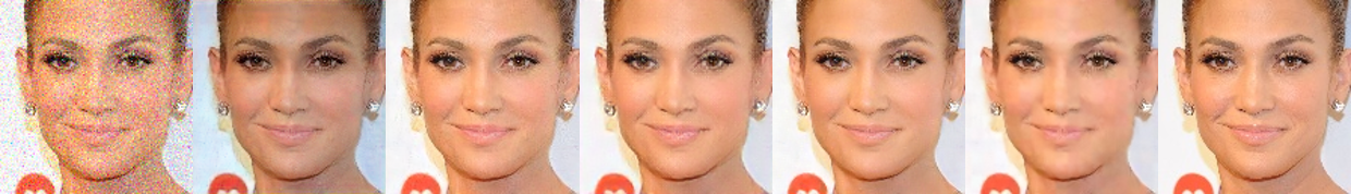
(b) Visual results of different methods for the Face Denoising task on the EDFace-Celeb-1M (BFR128) dataset

(c) Visual results of different methods for the Face Artifact Removal task on the EDFace-Celeb-1M (BFR128) dataset

(d) Visual results of different methods for the Face Super Resolution task on the EDFace-Celeb-1M (BFR128) dataset

(e) Visual results of different methods for the Blind Face Restoration task on the EDFace-Celeb-1M (BFR128) dataset

Figure 4: Visual results corresponding to different tasks on the EDFace-Celeb-1M (BFR128) dataset. From left to right: LQ image, results of HiFaceGAN[43], PSFR-GAN[45], GFP-GAN[46], GPEN[44], STUNet and HQ image.

TABLE V: Performance comparison of representative BFR methods on the EDFace-Celeb-150K (BFR512) dataset. Results are reported in terms of PSNR, SSIM, MS-SSIM, LPIPS, and NIQE metrics. The best and the second best performance results are marked with red and blue colors, respectively.

Task	Methods	PSNR↑	SSIM↑	MS-SSIM↑	LPIPS↓	NIQE↓
Face Deblurring	DFDNet [42]	25.4072	0.6512	0.8724	0.4008	7.8913
	HiFaceGAN [43]	26.7421	0.8095	0.9382	0.2029	16.6642
	PSFR-GAN [45]	27.4023	0.7604	0.9155	0.2292	17.4076
	GFP-GAN [46]	28.8166	0.7709	0.9180	0.1721	15.5942
	GPEN [44]	27.0658	0.7175	0.8928	0.2188	15.3187
	STUNet	29.5572	0.8052	0.9289	0.3381	14.7874
Face Denoising	DFDNet [42]	24.3618	0.5738	0.8423	0.3238	7.7809
	HiFaceGAN [43]	30.0409	0.8731	0.9563	0.1439	16.7363
	PSFR-GAN [45]	28.5397	0.8232	0.9390	0.2208	19.4719
	GFP-GAN [46]	33.2020	0.8711	0.9582	0.1259	15.8440
	GPEN [44]	32.3736	0.8517	0.9506	0.1555	15.6820
	STUNet	34.5500	0.8848	0.9587	0.1787	16.5480
Face Artifact Removal	DFDNet [42]	27.4781	0.7845	0.9409	0.2241	7.5553
	HiFaceGAN [43]	27.1164	0.8897	0.9635	0.1241	18.7117
	PSFR-GAN [45]	29.4285	0.9101	0.9719	0.1245	15.9760
	GFP-GAN [46]	35.7201	0.9144	0.9780	0.0842	16.8320
	GPEN [44]	33.8355	0.8701	0.9657	0.0986	16.9854
	STUNet	36.5017	0.9246	0.9799	0.1411	16.0487
Face Super Resolution	DFDNet [42]	26.8691	0.7405	0.9224	0.2620	7.4796
	HiFaceGAN [43]	26.6103	0.8480	0.9476	0.1681	15.8911
	PSFR-GAN [45]	33.1233	0.8588	0.9602	0.1331	16.7143
	GFP-GAN [46]	33.4217	0.8629	0.9610	0.1127	16.8970
	GPEN [44]	31.3507	0.8273	0.9501	0.1357	15.7813
	STUNet	33.9060	0.8809	0.9636	0.2235	17.0899
Blind Face Restoration	DFDNet [42]	23.9349	0.5573	0.8053	0.4231	9.0084
	HiFaceGAN [43]	25.3083	0.7260	0.8701	0.3012	14.7883
	PSFR-GAN [45]	26.2998	0.6934	0.8581	0.3167	17.1906
	GFP-GAN [46]	28.4809	0.7857	0.9255	0.2171	14.4933
	GPEN [44]	25.5778	0.6721	0.8448	0.3113	15.8422
	STUNet	27.1833	0.7346	0.8654	0.4457	17.0305

TABLE VI: Performance comparison of representative BFR methods on the EDFace-Celeb-150K (BFR512) dataset. Results are reported in terms of two task-driven metrics including AFLD and AFICS. The best and the second best performance results are marked with red and blue colors, respectively.

Task	Methods	AFLD↓	AFICS↑
Face Deblurring	DFDNet [42]	0.0221	0.8618
	HiFaceGAN [43]	0.0177	0.9673
	PSFR-GAN [45]	0.0191	0.9609
	GFP-GAN [46]	0.0186	0.9714
	GPEN [44]	0.0201	0.9554
	STUNet	0.0207	0.9644
Face Denoising	DFDNet [42]	0.0262	0.9062
	HiFaceGAN [43]	0.0168	0.9650
	PSFR-GAN [46]	0.0175	0.9575
	GFP-GAN [46]	0.0169	0.9657
	GPEN [44]	0.0173	0.9623
	STUNet	0.0450	0.9708
Face Artifact Removal	DFDNet [42]	0.0199	0.9433
	HiFaceGAN [43]	0.0166	0.9743
	PSFR-GAN [46]	0.0161	0.9748
	GFP-GAN [46]	0.0162	0.9792
	GPEN [44]	0.0167	0.9751
	STUNet	0.0175	0.9794
Face Super Resolution	DFDNet [42]	0.0201	0.9431
	HiFaceGAN [43]	0.0173	0.9584
	PSFR-GAN [46]	0.0166	0.9721
	GFP-GAN [46]	0.0164	0.9745
	GPEN [44]	0.0172	0.9698
	STUNet	0.0174	0.9763
Blind Face Restoration	DFDNet [42]	0.0247	0.8440
	HiFaceGAN [43]	0.0208	0.8918
	PSFR-GAN [46]	0.0212	0.8964
	GFP-GAN [46]	0.0186	0.9536
	GPEN [44]	0.0221	0.8782
	STUNet	0.0326	0.9045

We first evaluate these methods and our proposed STUNet on the EDFace-Celeb-1M (BFR128) to study their performance in the scenarios of several types of degradations when the low-quality input images are of resolution $128\times 128$.

Table III reports the comparison results of five methods, including our proposed STUNet. In the table, Face Deblurring, Face Denoising, Face Artifact Removal, Face Super-Resolution, and Blind Face Restoration are the five face restoration tasks corresponding to the degradation settings of Blur, Noise, JPEG, LR, and Full, respectively. PSNR, SSIM, and MS-SSIM are the three full-reference quantitative metrics. LPIPS and NIQE are the two non-reference quantitative metrics. The results in red color and blue color represent the best and the second best results.

We have the following findings regarding the results of different methods on the five tasks from Table III. 1) In terms of the full-reference quantitative metrics including PSNR, SSIM, and MS-SSIM, our STUNet achieves the best (face denoising, face artifact removal, and face super resolution) or the second best performance (face deblurring and blind face restoration), consistently beating other compared methods. Additionally, PSFR-GAN performs best for the task of face deblurring, and the second best for the face artifact removal task. HiFaceGAN, GFP-GAN and GPEN perform favourably, but not as well as STUNet and PSFR-GAN. 2) For the two non-reference quantitative metrics (LPIPS, and NIQE), GFP-GAN and GPEN achieve the best or the second best individually in tasks, but none of them demonstrates a significant advantage over the other. The HiFaceGAN and PSFR-GAN do not show competitive results against these two methods and perform better than ours. We suspect that the observed distinct characteristics of our proposed STUNet and the compared methods can be attributed to the different nature of our method and its counterparts. All the compared methods, HiFaceGAN, PSFR-GAN, GFP-GAN and GPEN, belongs to GAN-based ones. It is well known that GAN-type methods are strong at generating content pleasing human visual perception, which will naturally gain advantages over our method in the case of non-reference quantitative metrics. Our method pays more attention to important features by computing the self-attention to introduce connections between features. Thus it outperforms other compared methods in terms of full-reference quantitative metrics.

In addition, we also evaluate the performance of these methods with the two task-driven metrics of AFLD and AFICS. As shown in Table IV, regarding the AFLD metric, the best performance of different tasks is achieved by different methods, PSFR-GAN (face deblurring), STUNet (face denoising and face artifact removal), and HiFaceGAN (face super resolution and blind face restoration). The results indicate that STUNet and HiFaceGAN demonstrate the better ability in restoring LQ face images in various conditions, as they both achieve the best performance on two tasks. Besides, PSFR-GAN achieves the best performance on the face deblurring task and achieves the second-best performance for the face artifact removal task. GFP-GAN and GPEN obtain only the second-best performance at one or two tasks, which are not as satisfactory as the other three methods. In terms of the AFICS metric, our STUNet achieves the best performance at tasks of face denoising, face artifact removal, and blind face restoration, and obtains the second best performance for the task of face super resolution. The improvement over other methods shows its advantages. In addition, HiFaceGAN and PSFR-GAN achieve the best and second-best performance for tasks, none of them showing advance over each other. Moreover, the GFP-GAN and GPEN fail to achieve the best or the second-best performance for any task. Considering that our STUNet achieves outstanding performance at three full-referenced metrics (PSNR, SSIM, and MS-SSIM), the images generated by STUNet are more similar to the original image at the pixel level and show more utility in aiding the down-stream tasks like face recognition.

To evaluate the visual quality of results by different methods, we conduct a visual comparison of these state-of-the-art methods and the proposed STUNet in Fig. 4. It is difficult to find the difference among images generated by PSFR-GAN, GFP-GAN, and GPEN on Noise and JPEG settings corresponding to the tasks of face denoising and face artifact removal, though the results of every evaluation metric differ from each other, as Fig. 4(b), Fig. 4(c) show. Besides, on the most challenging setting Full, corresponding to the blind face restoration task, we find that the image recovered by GPEN is more satisfying to human visual perception, like Fig. 4(e). Regarding the two non-reference metrics in Table III, for the blind face restoration task, GPEN achieves a more satisfactory performance than other methods. Therefore, we suppose that the results of the non-reference metrics are better at reflecting whether the generated image satisfies the human visual perception.

5.4 EDFace-Celeb-150K (BFR512) Benchmark Results

To investigate the performance of these BFR methods when given input with a resolution of $512\times 512$, we carry out comparison studies among these methods and report the results in Table V. For the three full-referenced metrics (PSNR, SSIM, and MS-SSIM), similar to the results on the EDFace-Celeb-1M (BFR128) dataset, our STUNet is still the most competitive method among the six representative methods. STUNet achieves the best performance for face denoising, face artifact removal, and face super resolution tasks and achieves the second-best performance for the face deblurring task. Besides, GFP-GAN also shows satisfactory performance. It achieves the best performance for the blind face restoration task and the second-best performance for the tasks of face artifact removal and face super resolution. Among DFDNet, HiFaceGAN, PSFR-GAN, and GPEN, HiFaceGAN obtains the highest scores on several metrics for tasks. The other three methods achieve neither the best nor the second best on any task, not as well as the HiFaceGAN. Among the two non-reference metrics (LPIPS and NIQE), regarding the LPIPS metric, GFP-GAN stands out as the best performer across all the tasks. According to the scores of the NIQE metric, DFDNet outperforms other methods for all the tasks.

(a) Visual results of different methods for the Face Deblurring task on the EDFace-Celeb-150K (BFR512)

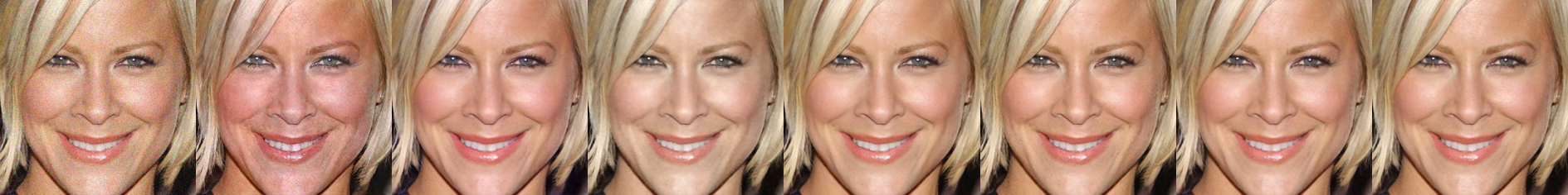
(b) Visual results of different methods for the Face Denoising task on the EDFace-Celeb-150K (BFR512)

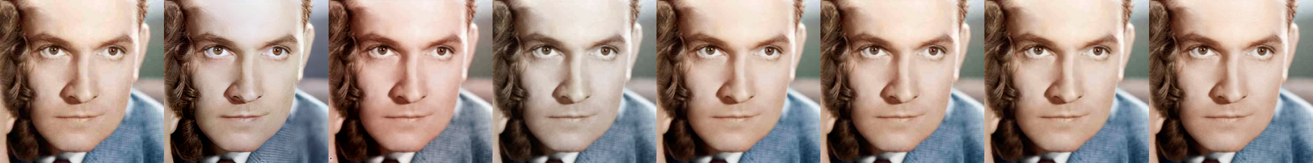
(c) Visual results of different methods for the Face Artifact Removal task on the EDFace-Celeb-150K (BFR512)

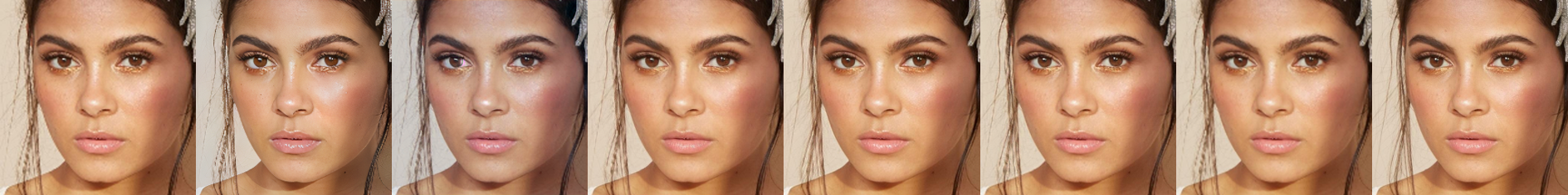
(d) Visual results of different methods for the Face Super Resolution task on the EDFace-Celeb-150K (BFR512)

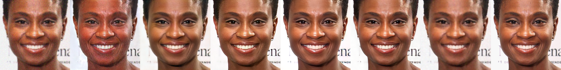
(e) Visual results of different methods for the Blind Face Restoration task on the EDFace-Celeb-150K (BFR512)

Figure 5: Visual results corresponding to different tasks on the EDFace-Celeb-150K (BFR512) dataset . From left to right: LQ image, results of DFDNet[42], HiFaceGAN[43], PSFR-GAN[45], GFP-GAN[46], GPEN[44], STUNet and HQ image.

(a) Visual results of different methods with 128$\times$128 real-world input.

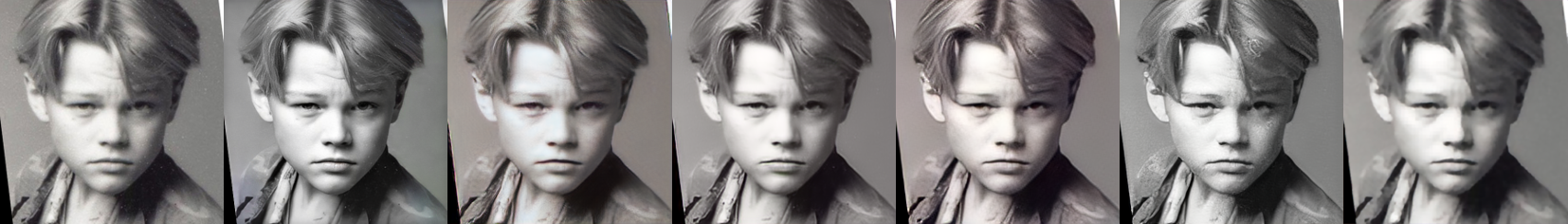
(b) Visual results of different methods with 512$\times$512 real-world input.

Figure 6: Visual results of different methods on the real-world dataset. From left to right: LQ image, results of DFDNet[42] (only showed in the bottom row), HiFaceGAN[43], PSFR-GAN[45], GFP-GAN[46], GPEN[44] and ours.

We also use the two task-driven metrics, AFLD and AFICS, to further evaluate the performance of these methods on the EDFace-Celeb-150K (BFR512) dataset. Table VI shows the quantitative results of these methods. For the AFLD metric, HiFaceGAN, PSFR-GAN, and GFP-GAN obtaining the best or the second best for different tasks perform more competitively than DFDNet, GPEN, and STUNet. Regarding the metric of AFICS, the proposed STUNet achieves the best performance for three tasks (face denoising, face artifact removal, and face super resolution) and the second best performance for the blind face restoration task. GFP-GAN achieves the best performance for two tasks (face deblurring and blind face restoration) and the second best performance for three tasks (face denoising, face artifact removal, and face super resolution). Besides, HiFaceGAN gains the second best performance for the face deblurring task. The other three methods do not achieve the best or the second best performance at any task. We suspect that the images recovered by the proposed STUNet and GFP-GAN are beneficial to improve the accuracy of face recognition.

Fig. 5 shows the visual comparison between these methods on the EDFace-Celeb-150K (BFR512) dataset. Similarly, as shown in Fig. 5(b) and Fig. 5(c), for the Noise and JPEG settings, it is difficult to find the difference between the images recovered by GFP-GAN and GPEN. Though the methods have achieved strong quantitative results, there is still a gap between the recovered images and the HQ images in terms of facial details and textures, as shown in Fig. 5(e).

5.5 Results on Real-World Dataset

Moreover, we evaluate the performance of the representative state-of-the-art methods on a real-world dataset. The visual comparison of these methods on the real-world dataset is displayed in Fig. 6. As shown in Fig. 6(a), the image recovered by GPEN has clearer facial textures, but the image recovered by PSFR-GAN is more similar to the original image. Besides, Fig .6(b) shows that the visual result of GFP-GAN is more competitive.

6 Conclusion and Future Directions

In this paper, we first construct two blind face restoration benchmark datasets which contain five settings corresponding to five face restoration tasks. Both the two datasets include large-scale pairs of LQ and HQ images and a fixed division of training and testing samples. Besides, we benchmark five existing blind face restoration methods on the proposed datasets and carry out a comprehensive comparison employing as many as eight quantitative metrics, including reference metrics, non-reference metrics, and task-driven metrics. Last, we propose a baseline model for blind face restoration called STUNet. The model is the first to introduce a self-attention mechanism into the blind face restoration task and achieves satisfactory performance.

In the future, we will study more settings such as BD, and DN, where “B” denotes blur operation, “N” denotes the operation of adding noise, and “D” stands for downsampling, to further explore the performance of different BFR methods. In addition, we will also explore new methods for blind face restoration.

References

- [1] Z. Shen, W.-S. Lai, T. Xu, J. Kautz, and M.-H. Yang, “Deep semantic face deblurring,” in Proceedings of the IEEE conference on computer vision and pattern recognition, 2018, pp. 8260–8269.
- [2] L. Chen, J. Pan, and Q. Li, “Robust face image super-resolution via joint learning of subdivided contextual model,” IEEE Transactions on Image Processing, vol. 28, no. 12, pp. 5897–5909, 2019.
- [3] M. Zhang, L. Huang, and M. Zhu, “Occluded face restoration based on generative adversarial networks,” in 2020 3rd International Conference on Advanced Electronic Materials, Computers and Software Engineering (AEMCSE). IEEE, 2020, pp. 315–319.
- [4] Z. Yue, H. Yong, Q. Zhao, D. Meng, and L. Zhang, “Variational denoising network: Toward blind noise modeling and removal,” Advances in neural information processing systems, vol. 32, 2019.
- [5] S. Anwar and N. Barnes, “Real image denoising with feature attention,” in Proceedings of the IEEE/CVF international conference on computer vision, 2019, pp. 3155–3164.
- [6] C. Dong, C. C. Loy, K. He, and X. Tang, “Image super-resolution using deep convolutional networks,” IEEE transactions on pattern analysis and machine intelligence, vol. 38, no. 2, pp. 295–307, 2015.
- [7] Y. Chen, Y. Tai, X. Liu, C. Shen, and J. Yang, “Fsrnet: End-to-end learning face super-resolution with facial priors,” in Proceedings of the IEEE Conference on Computer Vision and Pattern Recognition, 2018, pp. 2492–2501.
- [8] B. Lim, S. Son, H. Kim, S. Nah, and K. Mu Lee, “Enhanced deep residual networks for single image super-resolution,” in Proceedings of the IEEE conference on computer vision and pattern recognition workshops, 2017, pp. 136–144.
- [9] X. Wang, K. Yu, S. Wu, J. Gu, Y. Liu, C. Dong, Y. Qiao, and C. Change Loy, “Esrgan: Enhanced super-resolution generative adversarial networks,” in Proceedings of the European conference on computer vision (ECCV) workshops, 2018, pp. 0–0.
- [10] W. Yang, X. Zhang, Y. Tian, W. Wang, J.-H. Xue, and Q. Liao, “Deep learning for single image super-resolution: A brief review,” IEEE Transactions on Multimedia, vol. 21, no. 12, pp. 3106–3121, 2019.
- [11] C. Dong, Y. Deng, C. C. Loy, and X. Tang, “Compression artifacts reduction by a deep convolutional network,” in Proceedings of the IEEE international conference on computer vision, 2015, pp. 576–584.
- [12] K. Zhang, D. Li, W. Luo, J. Liu, J. Deng, W. Liu, and S. Zafeiriou, “Edface-celeb-1m: Benchmarking face hallucination with a million-scale dataset,” IEEE Transactions on Pattern Analysis and Machine Intelligence, 2022.
- [13] Z. Liu, Y. Lin, Y. Cao, H. Hu, Y. Wei, Z. Zhang, S. Lin, and B. Guo, “Swin transformer: Hierarchical vision transformer using shifted windows,” in Proceedings of the IEEE/CVF International Conference on Computer Vision, 2021, pp. 10 012–10 022.
- [14] T. Karras, S. Laine, and T. Aila, “A style-based generator architecture for generative adversarial networks,” in Proceedings of the IEEE/CVF conference on computer vision and pattern recognition, 2019, pp. 4401–4410.
- [15] D. Yi, Z. Lei, S. Liao, and S. Z. Li, “Learning face representation from scratch,” arXiv preprint arXiv:1411.7923, 2014.
- [16] Q. Cao, L. Shen, W. Xie, O. M. Parkhi, and A. Zisserman, “Vggface2: A dataset for recognising faces across pose and age,” in 2018 13th IEEE international conference on automatic face & gesture recognition (FG 2018). IEEE, 2018, pp. 67–74.
- [17] R. Rothe, R. Timofte, and L. V. Gool, “Dex: Deep expectation of apparent age from a single image,” in IEEE International Conference on Computer Vision Workshops (ICCVW), December 2015.
- [18] Z. Liu, P. Luo, X. Wang, and X. Tang, “Deep learning face attributes in the wild,” in Proceedings of the IEEE international conference on computer vision, 2015, pp. 3730–3738.
- [19] V. Le, J. Brandt, Z. Lin, L. Bourdev, and T. S. Huang, “Interactive facial feature localization,” in European conference on computer vision. Springer, 2012, pp. 679–692.
- [20] G. B. Huang, M. Mattar, T. Berg, and E. Learned-Miller, “Labeled faces in the wild: A database forstudying face recognition in unconstrained environments,” in Workshop on faces in’Real-Life’Images: detection, alignment, and recognition, 2008.
- [21] O. Jesorsky, K. J. Kirchberg, and R. W. Frischholz, “Robust face detection using the hausdorff distance,” in International conference on audio-and video-based biometric person authentication. Springer, 2001, pp. 90–95.
- [22] M. Koestinger, P. Wohlhart, P. M. Roth, and H. Bischof, “Annotated facial landmarks in the wild: A large-scale, real-world database for facial landmark localization,” in 2011 IEEE international conference on computer vision workshops (ICCV workshops). IEEE, 2011, pp. 2144–2151.
- [23] Y. Sun, Y. Chen, X. Wang, and X. Tang, “Deep learning face representation by joint identification-verification,” Advances in neural information processing systems, vol. 27, 2014.
- [24] K. Zhang, W. Luo, Y. Zhong, L. Ma, W. Liu, and H. Li, “Adversarial spatio-temporal learning for video deblurring,” IEEE Transactions on Image Processing, vol. 28, no. 1, pp. 291–301, 2018.
- [25] K. Zhang, W. Luo, Y. Zhong, L. Ma, B. Stenger, W. Liu, and H. Li, “Deblurring by realistic blurring,” in Proceedings of the IEEE/CVF Conference on Computer Vision and Pattern Recognition, 2020, pp. 2737–2746.
- [26] O. Kupyn, V. Budzan, M. Mykhailych, D. Mishkin, and J. Matas, “Deblurgan: Blind motion deblurring using conditional adversarial networks,” in Proceedings of the IEEE conference on computer vision and pattern recognition, 2018, pp. 8183–8192.
- [27] O. Kupyn, T. Martyniuk, J. Wu, and Z. Wang, “Deblurgan-v2: Deblurring (orders-of-magnitude) faster and better,” in Proceedings of the IEEE/CVF International Conference on Computer Vision, 2019, pp. 8878–8887.
- [28] K. Zhang, W. Zuo, Y. Chen, D. Meng, and L. Zhang, “Beyond a gaussian denoiser: Residual learning of deep cnn for image denoising,” IEEE transactions on image processing, vol. 26, no. 7, pp. 3142–3155, 2017.
- [29] K. Zhang, W. Zuo, and L. Zhang, “Ffdnet: Toward a fast and flexible solution for cnn-based image denoising,” IEEE Transactions on Image Processing, vol. 27, no. 9, pp. 4608–4622, 2018.
- [30] Y. Zhang, K. Li, K. Li, L. Wang, B. Zhong, and Y. Fu, “Image super-resolution using very deep residual channel attention networks,” in Proceedings of the European conference on computer vision (ECCV), 2018, pp. 286–301.
- [31] C. Ledig, L. Theis, F. Huszár, J. Caballero, A. Cunningham, A. Acosta, A. Aitken, A. Tejani, J. Totz, Z. Wang et al., “Photo-realistic single image super-resolution using a generative adversarial network,” in Proceedings of the IEEE conference on computer vision and pattern recognition, 2017, pp. 4681–4690.
- [32] M. S. Sajjadi, B. Scholkopf, and M. Hirsch, “Enhancenet: Single image super-resolution through automated texture synthesis,” in Proceedings of the IEEE International Conference on Computer Vision, 2017, pp. 4491–4500.
- [33] K. Zhang, D. Li, W. Luo, W. Ren, B. Stenger, W. Liu, H. Li, and M.-H. Yang, “Benchmarking ultra-high-definition image super-resolution,” in Proceedings of the IEEE/CVF International Conference on Computer Vision, 2021, pp. 14 769–14 778.
- [34] X. Fu, Z.-J. Zha, F. Wu, X. Ding, and J. Paisley, “Jpeg artifacts reduction via deep convolutional sparse coding,” in Proceedings of the IEEE/CVF International Conference on Computer Vision, 2019, pp. 2501–2510.
- [35] Q. Cao, L. Lin, Y. Shi, X. Liang, and G. Li, “Attention-aware face hallucination via deep reinforcement learning,” in Proceedings of the IEEE Conference on Computer Vision and Pattern Recognition, 2017, pp. 690–698.
- [36] D. Kim, M. Kim, G. Kwon, and D.-S. Kim, “Progressive face super-resolution via attention to facial landmark,” arXiv preprint arXiv:1908.08239, 2019.
- [37] S. Menon, A. Damian, S. Hu, N. Ravi, and C. Rudin, “Pulse: Self-supervised photo upsampling via latent space exploration of generative models,” in Proceedings of the ieee/cvf conference on computer vision and pattern recognition, 2020, pp. 2437–2445.
- [38] H. Huang, R. He, Z. Sun, and T. Tan, “Wavelet-srnet: A wavelet-based cnn for multi-scale face super resolution,” in Proceedings of the IEEE International Conference on Computer Vision, 2017, pp. 1689–1697.
- [39] X. Yu and F. Porikli, “Hallucinating very low-resolution unaligned and noisy face images by transformative discriminative autoencoders,” in Proceedings of the IEEE Conference on Computer Vision and Pattern Recognition, 2017, pp. 3760–3768.
- [40] X. Yu, B. Fernando, R. Hartley, and F. Porikli, “Super-resolving very low-resolution face images with supplementary attributes,” in Proceedings of the IEEE conference on computer vision and pattern recognition, 2018, pp. 908–917.
- [41] X. Li, M. Liu, Y. Ye, W. Zuo, L. Lin, and R. Yang, “Learning warped guidance for blind face restoration,” in Proceedings of the European conference on computer vision (ECCV), 2018, pp. 272–289.
- [42] X. Li, C. Chen, S. Zhou, X. Lin, W. Zuo, and L. Zhang, “Blind face restoration via deep multi-scale component dictionaries,” in European Conference on Computer Vision. Springer, 2020, pp. 399–415.
- [43] L. Yang, S. Wang, S. Ma, W. Gao, C. Liu, P. Wang, and P. Ren, “Hifacegan: Face renovation via collaborative suppression and replenishment,” in Proceedings of the 28th ACM International Conference on Multimedia, 2020, pp. 1551–1560.
- [44] T. Yang, P. Ren, X. Xie, and L. Zhang, “Gan prior embedded network for blind face restoration in the wild,” in Proceedings of the IEEE/CVF Conference on Computer Vision and Pattern Recognition, 2021, pp. 672–681.
- [45] C. Chen, X. Li, L. Yang, X. Lin, L. Zhang, and K.-Y. K. Wong, “Progressive semantic-aware style transformation for blind face restoration,” in Proceedings of the IEEE/CVF Conference on Computer Vision and Pattern Recognition, 2021, pp. 11 896–11 905.
- [46] X. Wang, Y. Li, H. Zhang, and Y. Shan, “Towards real-world blind face restoration with generative facial prior,” in Proceedings of the IEEE/CVF Conference on Computer Vision and Pattern Recognition, 2021, pp. 9168–9178.
- [47] A. Vaswani, N. Shazeer, N. Parmar, J. Uszkoreit, L. Jones, A. N. Gomez, L. u. Kaiser, and I. Polosukhin, “Attention is all you need,” in Advances in Neural Information Processing Systems, I. Guyon, U. V. Luxburg, S. Bengio, H. Wallach, R. Fergus, S. Vishwanathan, and R. Garnett, Eds., vol. 30. Curran Associates, Inc., 2017. [Online]. Available: https://proceedings.neurips.cc/paper/2017/file/3f5ee243547dee91fbd053c1c4a845aa-Paper.pdf
- [48] N. Parmar, A. Vaswani, J. Uszkoreit, L. Kaiser, N. Shazeer, A. Ku, and D. Tran, “Image transformer,” in International Conference on Machine Learning. PMLR, 2018, pp. 4055–4064.
- [49] H. Hu, Z. Zhang, Z. Xie, and S. Lin, “Local relation networks for image recognition,” in Proceedings of the IEEE/CVF International Conference on Computer Vision, 2019, pp. 3464–3473.
- [50] P. Ramachandran, N. Parmar, A. Vaswani, I. Bello, A. Levskaya, and J. Shlens, “Stand-alone self-attention in vision models,” Advances in Neural Information Processing Systems, vol. 32, 2019.
- [51] H. Zhao, J. Jia, and V. Koltun, “Exploring self-attention for image recognition,” in Proceedings of the IEEE/CVF Conference on Computer Vision and Pattern Recognition, 2020, pp. 10 076–10 085.
- [52] R. Child, S. Gray, A. Radford, and I. Sutskever, “Generating long sequences with sparse transformers,” arXiv preprint arXiv:1904.10509, 2019.
- [53] D. Weissenborn, O. Täckström, and J. Uszkoreit, “Scaling autoregressive video models,” arXiv preprint arXiv:1906.02634, 2019.
- [54] J. Ho, N. Kalchbrenner, D. Weissenborn, and T. Salimans, “Axial attention in multidimensional transformers,” arXiv preprint arXiv:1912.12180, 2019.
- [55] H. Wang, Y. Zhu, B. Green, H. Adam, A. Yuille, and L.-C. Chen, “Axial-deeplab: Stand-alone axial-attention for panoptic segmentation,” in European Conference on Computer Vision. Springer, 2020, pp. 108–126.
- [56] J.-B. Cordonnier, A. Loukas, and M. Jaggi, “On the relationship between self-attention and convolutional layers,” arXiv preprint arXiv:1911.03584, 2019.
- [57] A. Dosovitskiy, L. Beyer, A. Kolesnikov, D. Weissenborn, X. Zhai, T. Unterthiner, M. Dehghani, M. Minderer, G. Heigold, S. Gelly et al., “An image is worth 16x16 words: Transformers for image recognition at scale,” arXiv preprint arXiv:2010.11929, 2020.
- [58] H. Touvron, M. Cord, M. Douze, F. Massa, A. Sablayrolles, and H. Jégou, “Training data-efficient image transformers & distillation through attention,” in International Conference on Machine Learning. PMLR, 2021, pp. 10 347–10 357.
- [59] J. Cao, Y. Li, K. Zhang, and L. Van Gool, “Video super-resolution transformer,” arXiv preprint arXiv:2106.06847, 2021.
- [60] H. Chen, Y. Wang, T. Guo, C. Xu, Y. Deng, Z. Liu, S. Ma, C. Xu, C. Xu, and W. Gao, “Pre-trained image processing transformer,” in Proceedings of the IEEE/CVF Conference on Computer Vision and Pattern Recognition, 2021, pp. 12 299–12 310.
- [61] Z. Wang, X. Cun, J. Bao, and J. Liu, “Uformer: A general u-shaped transformer for image restoration,” arXiv preprint arXiv:2106.03106, 2021.
- [62] J. Liang, J. Cao, G. Sun, K. Zhang, L. Van Gool, and R. Timofte, “Swinir: Image restoration using swin transformer,” in Proceedings of the IEEE/CVF International Conference on Computer Vision, 2021, pp. 1833–1844.
- [63] A. Vaswani, N. Shazeer, N. Parmar, J. Uszkoreit, L. Jones, A. N. Gomez, Ł. Kaiser, and I. Polosukhin, “Attention is all you need,” Advances in neural information processing systems, vol. 30, 2017.