Lower Bounds and Nearly Optimal Algorithms in Distributed Learning with Communication Compression

Abstract

Recent advances in distributed optimization and learning have shown that communication compression is one of the most effective means of reducing communication. While there have been many results on convergence rates under communication compression, a theoretical lower bound is still missing.

Analyses of algorithms with communication compression have attributed convergence to two abstract properties: the unbiased property or the contractive property. They can be applied with either unidirectional compression (only messages from workers to server are compressed) or bidirectional compression. In this paper, we consider distributed stochastic algorithms for minimizing smooth and non-convex objective functions under communication compression. We establish a convergence lower bound for algorithms whether using unbiased or contractive compressors in unidirection or bidirection. To close the gap between the lower bound and the existing upper bounds, we further propose an algorithm, NEOLITHIC, which almost reaches our lower bound (up to logarithm factors) under mild conditions. Our results also show that using contractive bidirectional compression can yield iterative methods that converge as fast as those using unbiased unidirectional compression. The experimental results validate our findings.

1 Introduction

Large-scale optimization is a critical step in many machine learning applications. Millions or even billions of data samples contribute to the excellent performance in tasks such as robotics, computer vision, natural language processing, healthcare, and so on. However, such a scale of data samples and model parameters leads to enormous communication that hampers the scalability of distributed machine-learning training systems. We urgently need communication-reduction strategies. State-of-the-art strategies include communication compression [4, 12, 56], decentralized communication [38, 9, 20], lazy communication [57, 32, 19], and beyond. This article will focus on the former.

The most common method of distributed training is Parallel SGD (P-SGD) [15]. In P-SGD, the stochastic gradients that workers transmit to a server cause significant communication overhead in large-scale machine learning. To reduce this overhead, many recent works propose to compress the messages sent unidirectionally from workers to server [5, 28, 4] or compress the messages between them bidirectionally [62, 70]. The method of compression is either sparsification or quantization [5, 28, 4] or their combination [28, 14]. The literature [58, 55, 62, 70] reveals that bidirectional compression can save more communication, but leads to slower convergence rates.

Although there are many specific compression methods, their convergence analyses are mainly built on unbiased compressibility or contractive compressibility. The literature [14, 54, 71] summarizes these two properties and how they appear in the analyses. An unbiased compressor compresses a vector $x$ into a quantized version $C(x)$ satisfying $\mathbb{E}[C(x)]=x$, i.e., no bias is introduced. The contractive compressor may introduce bias, but its compression introduces much less variance. We give their definitions below. Although the contractive compressor can empirically work better, the analysis based on the unbiased compressor yields faster convergence due to unbiasedness [14, 44, 29, 26].

Despite the quick progress made in compression techniques and their convergence, we do not yet understand the limits of algorithms with communication compression. Since unbiased and contractive compressibilities are the two representative characteristics, we use them to generally theorize two types of compressors. For each type, we intend to answer:

What is the optimal convergence rate that a distributed algorithm can achieve when using any compressor of this type?

Here, we assume that only unbiased compressibility or contractive compressibility can be utilized, not considering any additional special compressor design; after all, any special design in the literature has been heuristic, whose effectiveness can be explained at best and not proved or quantified. So, we further clarify our question: Given a class of optimization problems (specified below) and a type of compressors, if we choose the worst combination of them to defeat an algorithm, what will the convergence rate that the best-defending algorithm can reach? To our knowledge, they are fundamental questions not addressed yet.

Table 1: Comparison between various distributed stochastic algorithms with communication compression for non-convex loss functions. For clarity, we keep the stochastic gradient variance $\sigma^{2}$, data heterogeneity bound $b^{2}$ , gradient square norm bound $G^{2}$ (used in [58, 62, 68], much larger than $b^{2}$ and $L$) , but omit smoothness constant $L$, and initialization $f(x^{(0)})-f^{\star}$ in the below results. Moreover, notation $\tilde{O}(\cdot)$ hides all logarithmic terms. Notation $\delta$ and $\omega$ are compressor-related parameters (see detailed discussions in Section 2).

	Algorithm	Convergence Rate	Compressiona	Trans. Compl.b
Lower Bound	Theorem 1+Corollary 1	$\Omega\left(\frac{\sigma}{\sqrt{nT}}+\frac{1}{\delta T}\right)$	Uni/Bidirectional Contractive	$\Omega(n/\delta^{2})$
	Theorem 2+Corollary 2	$\Omega\left(\frac{\sigma}{\sqrt{nT}}+\frac{1+\omega}{T}\right)$	Uni/Bidirectional Unbiased	$\Omega\left(n(1+\omega)^{2}\right)$
Upper Bound	Theorem 3	$\tilde{O}\left(\frac{\sigma}{\sqrt{nT}}+\frac{1}{\delta T}\right)$	Uni/Bidirectional Contractive	$\tilde{O}(n/\delta^{2})$
	Corollary 3	$\tilde{O}\left(\frac{\sigma}{\sqrt{nT}}+\frac{1+\omega}{T}\right)$	Uni/Bidirectional Unbiased	$\tilde{O}(n(1+\omega)^{2})$
	Q-SGD [31]	$O\left(\frac{(1+\omega)^{1/2}\sigma+\omega^{1/2}b}{\sqrt{nT}}\right)^{\dagger,\diamond}$	Unidirectional i.i.d, Unbiased	$-$
	MEM-SGD [58]	$O\left(\frac{\sigma}{\sqrt{nT}}+\frac{G^{2/3}}{\delta^{2/3}T^{2/3}}+\frac{1}{T}\right)^{\diamond}$	Unidirectional Contractive	$O(n^{3}/\delta^{4})$
	Double-Squeeze [62]	$O\left(\frac{\sigma}{\sqrt{nT}}+\frac{G^{2/3}}{\delta^{4/3}T^{2/3}}+\frac{1}{T}\right)^{\diamond}$	Bidirectional Contractive	$O(n^{3}/\delta^{8})$
	CSER [68]	$O\left(\frac{\sigma}{\sqrt{nT}}+\frac{G^{2/3}}{\delta^{2/3}T^{2/3}}+\frac{1}{T}\right)^{\diamond}$	Unidirectional Contractive	$O(n^{3}/\delta^{4})$
	EF21-SGD [24]	$O\left(\frac{\sigma}{\sqrt{\delta^{3}T}}+\frac{1}{\delta T}\right)^{\ast}$	Unidirectional Contractive	$-$
a This column indicates the type of the compressor and in what direction the compression is applied.
b This column indicates the transient complexity, i.e., the number of gradient queries (or communication rounds)
the algorithm has to experience before reaching the linear-speedup stage, i.e., $O(\frac{\sigma}{\sqrt{nT}})$.
† This convergence rate is valid only for $T=\Omega(n(1+\frac{\omega}{n})^{2})$. Since the rate $\frac{(1+\omega)^{1/2}\sigma+\omega^{1/2}b}{\sqrt{nT}}$ is always worse than $\frac{\sigma}{\sqrt{nT}}$,
the transient complexity is not available.
∗ Since the convergence rate does not show linear-speedup, the transient complexity is not available
⋄ The rates are either strengthened by relaxing the original restrictive assumptions or extended to the same setting as
NEOLITHIC for a fair comparison, see more details in Appendix C.

1.1 Main Results

This paper clarifies these open questions by providing lower bounds under the non-convex smooth stochastic optimization setting, and developing effective algorithms that match the lower bounds up to logarithm factors. In particular, our contributions are:

• We establish convergence lower bounds for distributed algorithms with communication compression in the stochastic non-convex regime. Our lower bounds apply to any algorithm conducting unidirectional or bidirectional compression with unbiased or contractive compressors. We find a clear gap between the established lower bounds and the existing convergence rates.

• We propose a novel nearly optimal algorithm with compression (NEOLITHIC) to fill in this gap. NEOLITHIC can adopt either unidirectional or bidirectional compression, and is compatible with both unbiased and contractive compressors. Using any combination, NEOLITHIC provably matches the above lower bound, under an additional mild assumption and up to logarithmic factors.

• The convergence results of NEOLITHIC imply that algorithms using biased contractive compressors bidirectionally can theoretically converge as fast as those with unbiased compressors used unidirectionally (see discussion in Remark 2). Before out work, it is only established in [48] that, for convex problems and unbiased compressors, algorithms with bidirectional compression can match with the counterparts with unidirectional compression.

• We provide extensive experimental results to validate our theories.

All established results in this paper as well as convergence rates of existing state-of-the-art distributed algorithms with communication compression are listed in Table 1. The transient complexity, which measures how sensitive the algorithm is to the compression strategy (see Section 3), is also listed in the table. The smaller the transient complexity is, the faster the algorithm converges.

1.2 Related Works.

Distributed learning.

Distributed learning has been increasingly useful in training large-scale machine learning models [21]. It typically follows a centralized or decentralized setup. Centralized approaches [2, 37], with P-SGD as the representative, require a global averaging step per iteration in which all workers need to synchronize with a central server. Decentralized approaches, however, are based on neighborhood averaging in which each worker only needs to synchronize with its immediate neighbors. The local interaction between directly-connected workers can save remarkable communication overhead compared to the remote communication between a worker and the central server. Well-known decentralized algorithms include decentralized SGD [45, 18, 77, 76], D²[61, 74], and stochastic gradient tracking [69, 35, 3], and their momentum variants [39, 75]. The lazy communication [73, 57, 19] is also utilized to reduce communication overhead in which workers conduct multiple local updates before sending messages. Lazy communication is also widely used in federated learning [43, 57, 32].

Communication compression.

To alleviate the communication overhead when transmitting the full model or stochastic gradient in distributed learning, communication compression is proposed in literature with two mainstream approaches: quantization and sparsification. Quantization [31, 60, 80] is essentially an unbiased operator with random noise. For example, [56] develop Sign-SGD by using only $1$ bit for each entry whose convergence is studied in [12, 13, 66]. Q-SGD [4] , as a generalized variant of Sign-SGD, compresses each entry with more flexible bits and enables a trade-off between convergence rates and communication costs. Sparsification, on the other hand, amounts to a biased but contractive operator. [65] suggest randomly dropping entries to achieve a sparse vector to communicate, while [58] suggest to transmit a certain number of the largest elements of the full model or gradient. The theories behind contractive compressors are limited to those in [64, 40, 59] due to analysis challenges, and they are established with assumptions such as bounded gradients [82, 33] or quadratic loss functions [67]. More discussions on unbiased and biased compressors can be found in [14, 54, 53]. Communication compression can also be combined with other communication-saving techniques such as decentralization [41, 81].

Error compensation.

The error compensation (feedback) mechanism is introduced by [56] to mitigate the error caused by 1-bit quantization. [67] study SGD with error-compensated quantization for quadratic functions with convergence guarantees. [58] show that error compensation can reduce quantization-incurred errors for strongly convex loss functions in the single-node setting. However, their analysis is restricted to compressors with expectation compression error no larger than the magnitude of the input vector, which is not applicable to general contractive compressors, such as [12]. Error-compensated SGD is studied in [5] for non-convex loss functions with no establishment of an improved convergence rate. A recent work [52] gives the first algorithm EF21, in the deterministic regime, using unidirectional compression with contractive compressors that rely only on standard assumptions. The later work [24] extends EF21 to the stochastic regime but cannot show linear speedup in terms of the number of workers.

Lower bounds in optimization.

Lower bounds are well studied in convex optimization [23, 1, 22] especially when there is no gradient stochasticity [8, 78, 10, 6, 25]. In non-convex optimization, [16, 17] propose a zero-chain model and show a tight bound for first-order methods. By splitting the zero-chain model into multiple components, [83, 7] extend the approach to finite sum and stochastic problems. Recently, [42, 76] show the lower bounds in the decentralized stochastic setting by assigning disjoint components of the model to remote nodes in the graphs. For distributed learning with communication compression, a useful work [49] establishes a lower bound for unidirectional/bidirectional compression for strongly convex problems with fixed learning rates and unbiased compressors. There are limited studies on lower bounds for non-convex distributed learning with unbiased/contractive compressions.

2 Problem Setup

In this section, we introduce the notations and assumptions used throughout the paper. We consider standard distributed learning with $n$ parallel workers. The data in worker $i$ follow a local distribution $D_{i}$, which can be heterogeneous among all workers. These workers, together with a central parameter server, collaborate to train a model by solving

$$\min_{x\in\mathbb{R}^{d}}\quad f(x)=\frac{1}{n}\sum_{i=1}^{n}f_{i}(x)\quad\text{with}\quad f_{i}(x)=\mathbb{E}_{\xi_{i}\sim D_{i}}[F(x;\xi_{i})],$$ (1)

where $F(x;\xi)$ is the loss function evaluated at parameter $x$ with datapoint $\xi$. Since the objective $f$ can be non-convex, finding a global minimum of (1) is generally intractable. Therefore, we turn to seeking a model $\hat{x}$ with a small gradient magnitude in expectation, i.e., $\mathbb{E}[\|\nabla f(\hat{x})\|^{2}]$. Next we introduce the setup under which we study the convergence rate.

Function class.

We let the function class ${\mathcal{F}}_{\Delta,L}$ denote the set of all functions satisfying Assumption 1 for any underlying dimension $d\in\mathbb{N}_{+}$ and a given initialization point $x^{(0)}\in\mathbb{R}^{d}$.

Assumption 1 (Smoothness).

Each local objective $f_{i}$ has $L$-Lipschitz gradient, i.e.,

$$\left\|\nabla f_{i}(x)-\nabla f_{i}(y)\right\|\leq L\|x-y\|$$

for all $i\in\{1,\dots,n\},x,y\in\mathbb{R}^{d}$, and $f(x^{(0)})-\inf_{x\in\mathbb{R}^{d}}f(x)\leq\Delta$ with $f=\frac{1}{n}\sum_{i=1}^{n}f_{i}$.

Gradient oracle class.

We assume each worker $i$ has access to its local gradient $\nabla f_{i}(x)$ via a stochastic gradient oracle $O_{i}(x;\zeta_{i})$ subject to independent randomness $\zeta_{i}$, e.g., the mini-batch sampling $\zeta_{i}\triangleq\xi_{i}\sim D_{i}$. We further assume that the output $O_{i}(x,\zeta_{i})$ is an unbiased estimator of the full-batch gradient $\nabla f_{i}(x)$ with a bounded variance. Formally, we let the stochastic gradient oracle class $O_{\sigma^{2}}$ denote the set of all oracles $O_{i}$ satisfying Assumption 2.

Assumption 2 (Gradient stochasticity).

For any $x\in\mathbb{R}^{d}$, the independent oracles $\{O_{i}:1\leq i\leq n\}$ satisfy

$$\mathbb{E}_{\zeta_{i}}[O_{i}(x;\zeta_{i})]=\nabla f_{i}(x)\quad\text{ and }\quad\mathbb{E}_{\zeta_{i}}[\|O_{i}(x;\zeta_{i})-\nabla f_{i}(x)\|^{2}]\leq\sigma^{2},\quad\forall\,x\in\mathbb{R}^{d}\text{ and }i\in\{1,\dots,n\}.$$

Compressor class.

The two widely-studied classes of compressors in literature are i) the $\omega$-unbiased compressor, described by Assumption 3, e.g., the stochastic quantization operator [4], and ii) the $\delta$-contractive compressor, described by Assumption 4, e.g., the rand-$k$ [51] operator and top-$k$ operator [58, 51].

Assumption 3 (Unbiased compressor).

The (possibly random) compression operator $C:\mathbb{R}^{d}\rightarrow\mathbb{R}^{d}$ satisfies

$$\mathbb{E}[C(x)]=x,\quad\mathbb{E}[\|C(x)-x\|^{2}]\leq\omega\|x\|^{2},\quad\forall\,x\in\mathbb{R}^{d}$$

for constant $\omega\geq 0$, where the expectation is taken over the randomness of the compression operator $C$.

Assumption 4 (Contractive compressor).

The (possibly random) compression operator $C:\mathbb{R}^{d}\rightarrow\mathbb{R}^{d}$ satisfies

$$\mathbb{E}[\|C(x)-x\|^{2}]\leq(1-\delta)\|x\|^{2},\quad\forall\,x\in\mathbb{R}^{d}$$

for constant $\delta\in(0,1]$, where the expectation is taken over the randomness of the compression operator $C$.

We let ${\mathcal{U}}_{\omega}$ and ${\mathcal{C}}_{\delta}$ denote the set of all $\omega$-unbiased compressors and $\delta$-contractive compressors satisfying Assumptions 3 and 4, respectively. Note that the identity operator $I$ satisfies $I\in{\mathcal{U}}_{\omega}$ for all $\omega\geq 0$ and $I\in{\mathcal{C}}_{\delta}$ for all $\delta\in(0,1]$. Generally, an $\omega$-unbiased compressor is not necessarily contractive when $\omega$ is larger than $1$. However, since $C\in{\mathcal{U}}_{\omega}$ implies $(1+\omega)^{-1}C\in{\mathcal{C}}_{(1+\omega)^{-1}}$, the scaled unbiased compressor is contractive though the converse may not hold. Hence, the class of contractive compressors is strictly richer since it contains all unbiased compressors through scaling.

Algorithm class.

We consider a centralized and synchronous algorithm $A$ in which i) workers are allowed to communicate only directly with the central server but not between one another; ii) all iterations are synchronized, meaning that all workers start each of their iterations simultaneously. Each worker $i$ holds a local copy of the model, denoted by $x_{i}^{(t)}$, at iteration $t$. The output $\hat{x}^{(t)}$ of $A$ after $t$ iterations can be any linear combination of all previous local models, namely,

$$\hat{x}^{(t)}\in\mathrm{span}\left(\{x_{i}^{(s)}:0\leq s\leq t,\,1\leq i\leq n\}\right).$$

We further require algorithms $A$ to satisfy the so-called “zero-respecting” property, which appears in [16, 17, 42] (see formal definition in Appendix A.1). This property implies that the number of non-zero entries of the local model of a worker can be increased only by conducting local stochastic gradient queries or synchronizing with the server. The zero-respecting property holds with all algorithms in Table 1 and most first-order methods based on SGD [46, 34, 30, 79]. In addition to these properties, algorithm $A$ has to admit communication compression. Specifically, we endow the server with a compressor $C_{0}$ and each worker $i\in\{1,\cdots,n\}$ with a compressor $C_{i}$. If $C_{i}=I$ for some $i\in\{0,\cdots,n\}$, then worker $i$ (or the server if $i=0$) conducts lossless communication. When $C_{i}\neq I$ for any $i\in\{0,\cdots,n\}$, algorithm $A$ conducts bidirectional compression. When $C_{0}=I$, algorithm $A$ conducts unidirectional compression on messages from workers to server. The definition of the algorithm class with bidirectional/unidirectional compression is as follows.

Definition 1 (Algorithm class).

Given compressors $\{C_{0},C_{1},\dots,C_{n}\}$, write ${\mathcal{A}}^{B}_{\{C_{i}\}_{i=0}^{n}}$ for the set of all centralized, synchronous, zero-respecting algorithms admitting bidirectional compression in which i) compressor $C_{i}$, $\forall\,i\in\{1,\dots,n\}$, is applied to messages from worker $i$ to the server, and ii) compressor $C_{0}$ is applied to messages from the server to all workers.

When $C_{0}=I$, we write ${\mathcal{A}}^{B}_{\{C_{0}=I\}\cup\{C_{i}\}_{i=1}^{n}}$, or ${\mathcal{A}}^{U}_{\{C_{i}\}_{i=1}^{n}}$ for short, for the set of algorithms admitting unidirectional compression. The superscript $B$ or $U$ indicates “bidirectional” or “unidirectional”, respectively.

3 Lower Bounds

With all interested classes introduced above, we are ready to define the lower bound measure. Given local loss functions $\{f_{i}\}_{i=1}^{n}\subseteq{\mathcal{F}}_{\Delta,L}$, stochastic gradient oracles $\{O_{i}\}_{i=1}^{n}\subseteq{\mathcal{O}}_{\sigma^{2}}$ (with $O_{i}$ for worker $i$), compressors $\{{\mathcal{C}}_{i}\}_{i=0}^{n}\subseteq{\mathcal{C}}$ (with ${\mathcal{C}}$ being either ${\mathcal{U}}_{\omega}$ or ${\mathcal{C}}_{\delta}$), and an algorithm $A\in{\mathcal{A}}$ to solve problem (1) (with ${\mathcal{A}}$ being either ${\mathcal{A}}^{B}_{\{C_{i}\}_{i=0}^{n}}$ or ${\mathcal{A}}^{U}_{\{C_{i}\}_{i=1}^{n}}$), we let $\hat{x}_{{A},\{f_{i}\}_{i=1}^{n},\{O_{i}\}_{i=1}^{n},\{C_{i}\}_{i=0}^{n},T}$ denote the output of algorithm $A$ using no more than $T$ gradient queries and rounds of communication by each worker node. We define the minimax measure as

$$\inf_{A\in{\mathcal{A}}}\sup_{\{C_{i}\}_{i=0}^{n}\subseteq{\mathcal{C}}}\sup_{\{O_{i}\}_{i=1}^{n}\subseteq{\mathcal{O}}_{\sigma^{2}}}\sup_{\{f_{i}\}_{i=1}^{n}\subseteq{\mathcal{F}}_{\Delta,L}}\mathbb{E}[\|\nabla f(\hat{x}_{A,\{f_{i}\}_{i=1}^{n},\{O_{i}\}_{i=1}^{n},\{C_{i}\}_{i=0}^{n},T})\|^{2}].$$ (2)

In (2), we do not require the compressors $\{C_{i}\}_{i=0}^{n}$ to be distinct or independent. When ${\mathcal{C}}$ is ${\mathcal{U}}_{\omega}$ or ${\mathcal{C}}_{\delta}$, we allow the compressor parameter $\omega$ or $\delta$ to be accessible by algorithm $A$.

3.1 Unidirectional Unbiased Compresssion

Our first result is for algorithms that admit unidirectional compression and $\omega$-unbiased compressors.

Theorem 1 (Unidirectional unbiased compression).

For every $\Delta,\,L>0$, $n\geq 2$, $\omega\geq 0$, $\sigma>0$, $T\geq(1+\omega)^{2}$, there exists a set of local loss functions $\{f_{i}\}_{i=1}^{n}\subseteq\mathcal{F}_{\Delta,L}$, stochastic gradient oracles $\{O_{i}\}_{i=1}^{n}\subseteq\mathcal{O}_{\sigma^{2}}$, $\omega$-unbiased compressors $\{C_{i}\}_{i=0}^{n}\subseteq{\mathcal{U}}_{\omega}$ with $C_{0}=I$, such that for any algorithm $A\in\mathcal{A}^{U}_{\{C_{i}\}_{i=1}^{n}}$ starting from a given constant $x^{(0)}$, it holds that (proof is in Appendix A.3)

$$\mathbb{E}[\|\nabla f(\hat{x}_{A,\{f_{i}\}_{i=1}^{n},\{O_{i}\}_{i=1}^{n},\{C_{i}\}_{i=0}^{n},T})\|^{2}]=\Omega\left(\left(\frac{\Delta L\sigma^{2}}{nT}\right)^{\frac{1}{2}}+\frac{(1+\omega)\Delta L}{T}\right).$$ (3)

Consistency with previous works.

The bound in (3) is consistent with best-known lower bounds in different settings. When $\omega=0$, our result reduces to the tight bound for distributed training without compression [7]. When $n=1$ and $\omega=0$, our result reduces to the lower bound established in [7] under the single-node non-convex stochastic setting. When $n=1,\omega=0$ and $\sigma^{2}=0$, our result recovers the tight bound for deterministic non-convex optimization [16].

Linear-speedup.

When $T$ is sufficiently large, the first term $1/\sqrt{nT}$ dominates the lower bound (3). If an algorithm achieves an $O(1/\sqrt{nT})$ rate, it will require $T=O(1/(n\epsilon^{2}))$ gradient queries to reach a desired accuracy $\epsilon$, which is inversely proportional to $n$. Therefore, an algorithm achieves linear-speedup at $T$-th iteration if, for this $T$, the term involving $nT$ is dominating the rate.

Transient complexity.

Due to the compression-incurred overhead in convergence rate, a distributed stochastic algorithm with communication compression has to experience a transient stage to achieve its linear-speedup stage. Transient complexity are referred to the number of gradient queries (or communication rounds) when $T$ is relatively small so non-$nT$ terms still dominate the rate. The smaller the transient complexity is, the less gradient queries or communication rounds the algorithm requires to achieve linear-speedup stage. For example, if an algorithm can achieve the lower bound established in (3), it requires $(\frac{\Delta L\sigma^{2}}{nT})^{\frac{1}{2}}\geq\frac{(1+\omega)\Delta L}{T}$, i.e., $T=\Omega(n(1+\omega)^{2})$ transient gradient queries (or communication rounds) to achieve linear-speedup, which is proportional to the compression-related terms $(1+\omega)^{2}$. Here we mainly care about the orders with respect to $n$ and $\omega$ (or $\delta$ below) in transient complexity to evaluate how sensitive the algorithm is to compression. Transient complexity is also widely used in decentralized learning [50, 72] to gauge how network topology can influence the convergence rate.

3.2 Bidirectional Unbiased Compression

Theorem 1 applies to unidirectional compression where $C_{0}=I$. We next consider bidirectional compression with $C_{0}\in{\mathcal{U}}_{\omega}$. Since $\{C_{i}\}_{i=1}^{n}\subseteq{\mathcal{U}}_{\omega}$ with $C_{0}=I$ is a special case of $\{C_{i}\}_{i=0}^{n}\subseteq{\mathcal{U}}_{\omega}$, the lower bound for algorithms that admit bidirectional compression is greater than or equal to that with unidirectional compression by following the definition of the measure in (2).

Corollary 1 (Bidirectional unbiased compression).

Under the same setting as in Theorem 1, there exists a set of local objectives $\{f_{i}\}_{i=1}^{n}\subseteq\mathcal{F}_{\Delta,L}$, stochastic gradient oracles $\{O_{i}\}_{i=1}^{n}\subseteq\mathcal{O}_{\sigma^{2}}$, $\omega$-unbiased compressors $\{C_{i}\}_{i=0}^{n}\subseteq{\mathcal{U}}_{\omega}$ such that for any algorithm $A\in\mathcal{A}^{B}_{\{C_{i}\}_{i=0}^{n}}$ starting from $x^{(0)}$, the lower bound in (3) is also valid.

Theorem 1 and Corollary 1 indicate that distributed learning with both unidirectional and bidirectional communication compression share the same lower bound. It is intuitive since unidirectional compression is just a special case of bidirectional compression by letting $C_{0}=I$.

3.3 Unidirectional Contractive Compression

To obtain lower bounds for contractive compressors, we need the following lemma [54, Lemma 1].

Lemma 1 (Compressor relation).

It holds that $\delta\,{\mathcal{U}}_{\delta^{-1}-1}\triangleq\{\delta\,C:C\in{\mathcal{U}}_{\delta^{-1}-1}\}\subseteq{\mathcal{C}}_{\delta}$.

The above Lemma reveals that any $(\delta^{-1}-1)$-unbiased compressor is $\delta$-contractive when scaled by $\delta$. Therefore, if an algorithm $A$ admits all $\delta$-contractive compressors, it automatically admits all compressors in $\delta\,{\mathcal{U}}_{\delta^{-1}-1}$ due to Lemma 1. This relation, together with Theorem 1, helps us achieve the following lower bound with respect to $\delta$-contractive compressors.

Theorem 2 (Unidirectional contractive compression).

For every $\Delta,\,L>0$, $n\geq 2$, $0<\delta\leq 1$, $\sigma>0$, $T\geq\delta^{-2}$, there exists a set of loss objectives $\{f_{i}\}_{i=1}^{n}\subseteq\mathcal{F}_{\Delta,L}$, a set of stochastic gradient oracles $\{O_{i}\}_{i=1}^{n}\subseteq\mathcal{O}_{\sigma^{2}}$, a set of $\delta$-contractive compressors $\{C_{i}\}_{i=0}^{n}\subseteq{\mathcal{C}}_{\delta}$ with $C_{0}=I$, such that for any algorithm $A\in\mathcal{A}^{U}_{\{C_{i}\}_{i=0}^{n}}$ starting from $x^{(0)}$, it holds that (proof is in Appendix A.4)

$$\mathbb{E}[\|\nabla f(\hat{x}_{A,\{f_{i}\}_{i=1}^{n},\{O_{i}\}_{i=1}^{n},\{C_{i}\}_{i=0}^{n},T})\|^{2}]=\Omega\left(\left(\frac{\Delta L\sigma^{2}}{nT}\right)^{\frac{1}{2}}+\frac{\Delta L}{\delta T}\right).$$ (4)

Transient complexity. With the discussion on transient complexity in Section 3.1, it is easy to derive the transient iteration complexity as $\Omega(n/\delta^{2})$ for the lower bound with $\delta$-contractive compressors.

3.4 Bidirectional Contractive Compression

Noting that $\{C_{i}\}_{i=1}^{n}\subseteq{\mathcal{C}}_{\delta}$ with $C_{0}=I$ is a special case of $\{C_{i}\}_{i=0}^{n}\subseteq{\mathcal{C}}_{\delta}$, we can also establish the lower bound for algorithms that admit bidirectional compression and contractive compressors.

Corollary 2 (Bidirectional contractive compression).

Under the same settings as in Theorem 2, there exists a set of loss objectives $\{f_{i}\}_{i=1}^{n}\subseteq\mathcal{F}_{\Delta,L}$, a set of stochastic gradient oracles $\{O_{i}\}_{i=1}^{n}\subseteq\mathcal{O}_{\sigma^{2}}$, a set of $\delta$-contractive compressors $\{C_{i}\}_{i=1}^{n}\subseteq{\mathcal{C}}_{\delta}$, such that for any algorithm $A\in\mathcal{A}^{B}_{\{C_{i}\}_{i=0}^{n}}$ starting form $x^{(0)}$, the lower bound (4) is also valid.

4 NEOLITHIC: A Nearly Optimal Algorithm

Comparing the best-known upper bounds listed in Table 1 with the established lower bounds in (3) and (4), we find existing algorithms may be sub-optimal. There exists a clear gap between their convergence rates and our established lower bounds. In this section, we propose NEOLITHIC to fill in this gap. Its rate will match the lower bounds established in (3) and (4) up to logarithm factors. NEOLITHIC can work with both unidirectional and bidirectional compressions, and it is compatible with both unbiased and contractive compressors. NEOLITHIC will be discussed in detail with bidirectional contractive compression in this section. It is easy to be adapted to other settings by simply removing the compression on the server side or utilizing unbiased compressors with proper scaling.

Algorithm 1 Fast Compressed Communication: $v^{(k,R)}=\text{FCC}(v^{(k,\star)},C,R,\text{target receiver(s)})$

  Input: The vector $v^{(k,\star)}$ aimed to communicate at iteration $k$; a compressor $C$;

            rounds $R$; initial vector $v^{(k,0)}=0$; target receiver(s);

  for $r=0,\cdots,R-1$ do

     Compress $v^{(k,\star)}-v^{(k,r)}$ into $c^{(k,r)}=C(v^{(k,\star)}-v^{(k,r)})$

     Send $c^{(k,r)}$ to the target receiver(s)

     Update $v^{(k,r+1)}=v^{(k,r)}+c^{(k,r)}$

  end for$\hskip 105.98668pt\triangleright$ The set $\{c^{(k,r)}\}_{r=0}^{R-1}$ will be sent to the receiver during the for-loop

  return  Variable $v^{(k,R)}$. $\hskip 31.2982pt\triangleright$ It holds that $v^{(k,R)}=\sum_{r=0}^{R-1}c^{(k,r)}$

4.1 Fast Compressed Communication

NEOLITHIC is built on a communication compression module listed in Algorithm 1, which we call fast compressed communication (FCC). Given an input vector $v^{(k,\star)}$ to communicate in the $k$-th iteration, FCC first initializes $v^{(k,0)}=0$ and then recursively compresses the residual with $c^{(k,r)}\triangleq C(v^{(k,\star)}-v^{(k,r)})$ and sends it to the receiver for $R$ consecutive rounds, see the main recursion in Algorithm 1. When FCC module ends, the sender will transmit a set of compressed variables $\{c^{(k,r)}\}_{r=0}^{R-1}$ to the receiver, and return $v^{(k,R)}=\sum_{r=0}^{R-1}c^{(k,r)}$ to itself. Quantity $v^{(k,R)}$ can be regarded as a compressed vector of original input $v^{(k,\star)}$ after FCC operation.

FCC module can be conducted by the server (for which all variables in FCC are without any subscripts, e.g., $c^{(k,r)}$ and $v^{(k,r)}$) or by any worker $i$ (for which all variables are with a subscript $i$, e.g., $c_{i}^{(k,r)}$ and $v_{i}^{(k,r)}$). When $R=1$, FCC reduces to the standard compression utilized in existing literature [62, 58, 24, 68, 31]. While FCC requires $R$ rounds of communication per iteration, the following lemma establishes that the compression error decrease exponentially with respect to communication rounds $R$.

Lemma 2 (FCC property).

Let $C$ be a $\delta$-contractive compressor and $v^{(k,R)}=\mathrm{FCC}(v^{(k,\star)},C,R)$. It holds for any $R\geq 1$ and $v^{(k,\star)}\in\mathbb{R}^{d}$ that (proof is in Appendix B.1)

$$\mathbb{E}[\|v^{(k,R)}-v^{(k,\star)}\|^{2}]\leq(1-\delta)^{R}\|v^{(k,\star)}\|^{2},\quad\forall k=0,1,2,\cdots.$$ (5)

When $R=1$, the above FCC property (5) reduces to Assumption 4 for standard contractive compressors. When $R$ is large, FCC can output $v^{(k,R)}$ endowed with very small compression errors. The FCC protocol is also closely related to EF21 compression strategy [52]. However, the major novelty of FCC is to utilize multiple such compression rounds to help develop algorithms that can nearly match the established lower bounds.

4.2 NEOLITHIC Algorithm

NEOLITHIC is described in Algorithm 2. The FCC module in NEOLITHIC communicates $R$ rounds per iteration. To balance gradient queries and communication rounds, NEOLITHIC will query $R$ stochastic gradients per iteration, see the gradient accumulation step in Algorithm 2. Compared to other algorithms listed in Table 1, the proposed NEOLITHIC takes $R$ times more gradient queries and communication rounds than them per iteration. Given the same budgets to query gradient oracles and conduct communication as the other algorithms, say $T$ times on each worker, we shall consider $K=T/R$ iterations in NEOLITHIC for fair comparison.

Algorithm 2 NEOLITHIC

  Input: Initialize $x^{(0)}$; learning rate $\gamma$; compression round $R$; $\mathrm{er}^{(0)}=\mathrm{er}_{i}^{(0)}=0$, $\forall\,i\in[n]$

  for $k=0,1,\cdots,K-1$ do

     On all workers in parallel:

      Query stochastic gradients $\hat{g}_{i}^{(k)}=\frac{1}{R}\sum_{r=0}^{R-1}O_{i}(x^{(k)};\zeta_{i}^{(k,r)})$            $\triangleright$ Gradient accumulation

      Error compensate $\tilde{g}_{i}^{(k)}=\hat{g}_{i}^{(k)}+\mathrm{er}_{i}^{(k)}$

      Update error $\mathrm{er}_{i}^{(k+1)}=\tilde{g}_{i}^{(k)}-\text{FCC}(\tilde{g}_{i}^{(k)},C_{i},R,\text{server})$                 $\triangleright$ Worker sends $\{c_{i}^{(k,r)}\}$ to server

     On server:

      Error compensate $\tilde{g}^{(k)}=\frac{1}{n}\sum_{i=1}^{n}\sum_{r=0}^{R-1}c_{i}^{(k,r)}+\mathrm{er}^{(k)}$                   $\triangleright$ $\{c_{i}^{(k,r)}\}$ received from workers

      Update error ${\mathrm{er}}^{(k+1)}=\tilde{g}^{(k)}-\text{FCC}(\tilde{g}^{(k)},C_{0},R,\text{all workers})$          $\triangleright$ Server sends $\{c^{(k,r)}\}$ to workers

     On all workers in parallel:

      Update model parameter $x^{(k+1)}=x^{(k)}-\gamma\sum_{r=0}^{R-1}c^{(k,r)}$               $\triangleright$ $\{c^{(k,r)}\}$ received from server

  end for

We introduce the following assumption to establish the convergence rates of NEOLITHIC.

Assumption 5 (Gradient dissimilarity).

There exists some $b^{2}\geq 0$ such that

$$\frac{1}{n}\sum_{i=1}^{n}\|\nabla f_{i}(x)-\nabla f(x)\|^{2}\leq b^{2},\quad\forall\,x\in\mathbb{R}^{d}.$$

When local distributions $D_{i}$ are identical across all workers, we have $f_{i}(x)=f(x)$ for each $i\in\{1,\dots,n\}$ and the above assumption will always hold. We first establish the convergence rate of NEOLITHIC using bidirectional compression with contractive compressors.

Theorem 3 (NEOLITHIC with bidirectional contractive compression).

Given constants $n\geq 1$, $\delta\in(0,1]$ and Assumption 5, and let $x^{(k)}$ be generated by Algorithm 2. If $R=\lceil\frac{\max\{\ln\left({\delta T\max\{b^{2},\sigma^{2}\delta\}}/{\Delta L}\right),\ln(8)\}}{\delta}\rceil$ and the learning rate is set as in Appendix B.2, it holds for any $K\geq 0$ and compressors $\{C_{i}\}_{i=0}^{n}\subseteq{\mathcal{C}}_{\delta}$ that (proof is in Appendix B.2)

$$\frac{1}{K+1}\sum_{k=0}^{K}\mathbb{E}[\|\nabla f(x^{(k)})\|^{2}]=\tilde{O}\left(\left(\frac{\Delta L\sigma^{2}}{nT}\right)^{\frac{1}{2}}+\frac{\Delta L}{\delta T}\right),$$

where $T=KR$ is the total number of gradient queries/communication rounds on each worker and notation $\tilde{O}(\cdot)$ hides logarithmic factors. The above rate implies a transient complexity of $\tilde{O}(n\delta^{-2})$.

When $\{C_{i}\}_{i=0}^{n}$ are $\omega$-unbiased compressors, we utilize the fact that $(1+\omega)^{-1}C_{i}$ is $(1+\omega)^{-1}$-contractive for all $i\in\{0,\dots,n\}$ to derive that

Corollary 3 (NEOLITHIC with bidirectional unbiased compression).

Under the same assumptions as in Theorem 3, it holds for any $K\geq 0$ and compressors $\{C_{i}\}_{i=0}^{n}\subseteq{\mathcal{U}}_{\omega}$ that

$$\frac{1}{K+1}\sum_{k=0}^{K}\mathbb{E}[\|\nabla f(x^{(k)})\|^{2}]=\tilde{O}\left(\left(\frac{\Delta L\sigma^{2}}{nT}\right)^{\frac{1}{2}}+\frac{(1+\omega)\Delta L}{T}\right).$$

This further leads to a transient complexity of $\tilde{O}\left(n(1+\omega)^{2}\right)$.

Remark 1.

The convergence rates established in Theorem 3 and Corollary 3 are also valid for unidirectional compression when $C_{0}=I$. They can match the lower bounds established in Section 3 up to logarithm factors. Moreover, these rates are faster than other algorithms listed in Table 1.

Remark 2.

While our analysis relies on Assumption 5, the rates in Theorem 3 and Corollary 3 are polynomially independent of $b^{2}$. These results also imply that NEOLITHIC with bidirectional compression can perform as fast as its counterpart with unidirectional compression. In other words, imposing bidirectional compression can save communications in NEOLITHIC without hurting convergence rates. Before our work, it is established in literature [58, 55, 62, 70, 14] that bidirectional compression leads to slower convergence than unidirectional compression. Our results also imply that, given $\delta=(1+\omega)^{-1}$, well-designed algorithms such as NEOLITHIC with $\delta$-contractive compressors can converge as fast as their counterparts using $\omega$-unbiased compressors despite unbiasedness. Before our work, the analysis based on unbiased compressors [14, 44, 29, 26] exhibits theoretically faster convergence for non-convex problems.

Remark 3.

We remark that Assumption 5 is not required to obtain the lower bounds in Section 3. It is not known whether the lower bounds established in Section 3 can be achieved by NEOLITHIC when Assumption 5 does not hold. However, it is worth noting that Assumption 5 is already milder than those made in most works [82, 33, 58, 68, 62, 11] such as bounded gradients. To our best knowledge, only EF21-SGD [24] is guaranteed to converge without Assumption 5, which, however, leads to a fairly loose convergence rate (see Table 1) that cannot show linear-speedup $O(1/\sqrt{nT})$.

Remark 4.

In the deterministic scenario, i.e., $\sigma^{2}=0$, NEOLITHIC produces rate $\tilde{O}((1+\omega)\Delta L/T)$. There exist literature (e.g., [26, 63]) that can achieve rate $\tilde{O}((1+\omega/n)\Delta L/T)$ which outperforms NEOLITHIC especially when $\omega$ and $n$ are sufficiently large. However, this improvement is built upon an additional assumption that all local compressors $\{C_{i}\}_{i=0}^{n}$ are independent of each other and cannot share the same randomness. On the contrary, NEOLITHIC does not impose such an assumption and can be applied to both dependent and independent compressors.

5 Experiments

This section empirically investigates the performance of different compression algorithms with both synthetic simulation and deep learning tasks. We compare NEOLITHIC with P-SGD and its variants with communication compression: MEM-SGD, Double-Squeeze, and EF21-SGD.

5.1 Synthetic Datasets

Least square.

We consider the following least-square problem:

$$\min_{x\in\mathbb{R}^{d}}\quad\frac{1}{2n}\sum_{i=1}^{n}\|A_{i}x-b_{i}\|^{2},$$

where coefficient matrix $A_{i}\in\mathbb{R}^{M\times d}$ and measurement $b_{i}\in\mathbb{R}^{d}$ are associated with node $i$, and $M$ is the size of local dataset. We set $d=30$, $n=32$ and $M=1000$, and generate data by letting each node $i$ be associated with a local solution $x_{i}^{\star}$ randomly generated by ${\mathcal{N}}(0,I_{d})$. Then we generate each element in $A_{i}$ following standard normal distribution, and measurement $b_{i}$ is generated by $b_{i}=A_{i}x_{i}^{\star}+s_{i}$ with white noise $s_{i}\sim{\mathcal{N}}(0,0.01)$. At each query, every node will randomly sample a row in $A_{i}$ and the corresponding element in $b_{i}$ to evaluate the stochastic gradient. We adopt the rand-1 compressor and set the number of rounds $R=4$ for NEOLITHIC. e use stair-wise decaying learning rates in which the learning rates are divided by every $2,500$ communication rounds. Each algorithm is averaged with $20$ trials The result is shown in Figure 1 (left). It is observed that NEOLITHIC outperforms MEM-SGD and Double-Squeeze in convergence rate, and it performs closely to P-SGD.

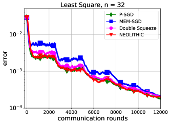
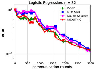
Figure 1: Convergence results on synthetic problems in terms of $\mathbb{E}[\|\nabla f(x)\|^{2}]$ versus communication rounds.

Logistic regression.

We consider the following logistic regression problem:

$$\min_{x\in\mathbb{R}^{d}}\quad\frac{1}{n}\sum_{i=1}^{n}f_{i}(x)\quad\text{ where }\quad f_{i}(x)=\frac{1}{M}\sum_{m=1}^{M}\ln\left(1+\exp\left(-y_{i,m}h_{i,m}^{\top}x\right)\right)$$

where $\{h_{i,m},y_{i,m}\}_{m=1}^{M}$ is the training dateset held by node $i$ in which $h_{i,m}\in\mathbb{R}^{d}$ with $d=30$ is a feature vector while $y_{i,m}\in\{-1,+1\}$ is the corresponding label. Similar to the least square problem, each node $i$ is associated with a local solution $x_{i}^{\star}$. We generate each feature vector $h_{i,m}\sim{\mathcal{N}}(0,I_{d})$, and label $y_{i,m}=1$ with probability $1/(1+\exp(-y_{i,m}h_{i,m}^{\top}x_{i}^{\star}))$; otherwise $y_{i,m}=-1$. At each query, every node will randomly sample a datapoint $(h_{i,m},y_{i,m})$ to evaluate the stochastic gradient. We adopt the rand-1 compressor and set the number of rounds $R=4$ for NEOLITHIC. We use stair-wise decaying learning rates in which the learning rates are divided by every $800$ communication rounds. Each algorithm is averaged with $20$ trials. The result is shown in Figure 1 (right). Again, NEOLITHIC outperforms MEM-SGD and Double-Squeeze in convergence rate, and it performs closely to P-SGD.

5.2 Deep Learning Tasks

Implementation details.

We implement all compression algorithms with PyTorch [47] 1.8.2 using NCCL 2.8.3 (CUDA 10.1) as the communication backend. For P-SGD, we used PyTorch’s native Distributed Data Parallel (DDP) module. All deep learning training scripts in this section run on a server with 8 NVIDIA V100 GPUs in our cluster and each GPU is treated as one worker.

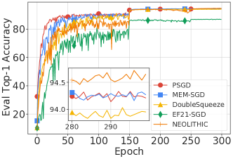
Figure 2: Convergence results on the CIFAR-10 in terms of training loss and validation accuracy.

Image classification.

We investigate the performance of the aforementioned methods with CIFAR-10 [36] dataset. For CIFAR-10 dataset, it consists of 50,000 training images and 10,000 validation images categorized in 10 classes. We utilize two common variants of ResNet [27] model on CIFAR-10 (ResNet-20 with roughly 0.27M parameters and ResNet-18 with 11.17M parameters). We train total 300 epochs and set the batch size to 128 on every worker. The learning rate is set to 5e-3 for single worker and warmed up in the first 5 epochs and decayed by a factor of 10 at 150 and 250-th epoch.

Table 2: Accuracy comparison with different algorithms on CIFAR-10 (8 workers, 5% compression ratio).

Methods	ResNet18	ResNet20
PSGD	93.99 ± 0.52	91.62 ± 0.13
MEM-SGD	94.35 ± 0.01	91.27 ± 0.08
Double-Squeeze	94.11 ± 0.14	90.73 ± 0.02
EF21-SGD	87.37 ± 0.49	65.82 ± 4.86
NEOLITHIC	94.63 ± 0.09	91.43 ± 0.10

All experiments were repeated three times with different seeds. For NEOLITHIC, we set $R=2$. Following previous works [62], we use top-$k$ compressor with different compression ratio to evaluate the performance of the aforementioned methods. As shown in Figure 2, Tables 2 and Table 3, NEOLITHIC consistently outperforms other compression methods and reaches the similar performance to P-SGD. It is worth noting that EF21-SGD, while guaranteed to converge with milder assumptions than ours, does not provide competitive performance in deep learning tasks listed in Tables 2, 3, and 4. We find our reported result for EF21-SGD is consistent with Figure 7 (the left plot) in [24].

Table 3: Accuracy comparison with different algorithms on CIFAR-10 (8 workers, 1% compression ratio).

Methods	ResNet18	ResNet20
MEM-SGD	93.99 ± 0.11	89.68 ± 0.17
Double-Squeeze	93.54 ± 0.17	89.35 ± 0.04
EF21-SGD	67.78 ± 2.14	56.0 ± 2.257
NEOLITHIC	94.155 ± 0.10	89.82 ± 0.37

The effect of compression ratio.

We also investigate the influence of different compression ratios. Table 3 is with a compression ratio of 1%, which indicates a harsher setting for compression methods. It is observed that NEOLITHIC still outperforms other compression methods.

Performance with heterogeneous data.

We simulate data heterogeneity among workers via a Dirichlet distribution-based partition with parameter $\alpha$ controlling the data heterogeneity. The training data for a particular class tends to concentrate in a single node as $\alpha\rightarrow 0$, i.e. becoming more heterogeneous, while the homogeneous data distribution is achieved as $\alpha\rightarrow\infty$. We test $\alpha=1$ and $10$ in Table 4 for all compared methods as corresponding to a setting with high/low heterogeneity.

Table 4: Accuracy comparison on CIFAR-10 with heterogeneous data (ResNet-20).

Methods	MEM-SGD	Double-Squeeze	EF21-SGD	NEOLITHIC	C-Ratio %
$\alpha=1$	85.42 ± 0.22	83.72 ± 0.17	38.5 ± 2.17	85.47 ± 0.12	1
$\alpha=10$	91.61 ± 0.19	91.25 ± 0.17	68.58 ± 0.13	91.76 ± 0.13	1
$\alpha=1$	86.43 ± 0.38	86.13 ± 0.21	72.65 ± 0.37	87.17 ± 0.24	5
$\alpha=10$	91.88 ± 0.23	91.66 ± 0.11	86.36 ± 0.15	92.14 ± 0.22	5

Effects of accumulation rounds.

We also empirically evaluate the performance of NEOLITHIC with different choice of parameter $R$ in deep learning tasks. NEOLITHIC have slightly performance degradation in both compression scenarios as $R$ scales up. We conjecture that the gradient accumulation step, which amounts to using large-batch samples in gradient evaluation, can help in the optimization and training stage as proved in this paper, but it may hurt the generalization performance. We recommend using NEOLITHIC in applications that are friendly to large-batch training.

Table 5: Effects of round numbers for CIFAR-10 dataset with ResNet-18

Rounds	2	3	4	5
NEOLITHIC (5%)	94.63 ± 0.09	93.32 ± 0.08	92.55 ± 0.12	91.48 ± 0.18
NEOLITHIC (1%)	94.16 ± 0.10	93.15 ± 0.11	92.27 ± 0.08	91.32 ± 0.12

6 Conclusion

This paper provides lower bounds for distributed algorithms with communication compression, whether the compression is unidirectional or bidirectional and unbiased or contractive. An algorithm called NEOLITHIC is introduced to match the lower bounds under the assumption of bounded gradient dissimilarity. Future directions include developing optimal algorithms without the assumption, as well as discovering additional compression properties that might produce a better lower bound.

Appendix A Lower Bounds

In this section, we provide the proofs for Theorem 1 and 2. To proceed, we first introduce the zero-respecting property and zero-chain functions.

A.1 Zero-Respecting Algorithms

Let $[x]_{j}$ denote the $j$-th coordinate of a vector $x\in\mathbb{R}^{d}$ for $j=1,\dots,d$, and define $\mathrm{prog}(x)$ as

$$\mathrm{prog}(x):=\begin{cases}0&\text{if $x=0$};\\ \max_{1\leq j\leq d}\{j:[x]_{j}\neq 0\}&\text{otherwise}.\end{cases}$$ (6)

Similarly, for a set of points ${\mathcal{X}}=\{x_{1},x_{2},\dots\}$, we define $\mathrm{prog}({\mathcal{X}}):=\max_{x\in{\mathcal{X}}}\mathrm{prog}(x)$. Apparently, it holds that $\mathrm{prog}({\mathcal{X}}\cup{\mathcal{Y}})=\max\{\mathrm{prog}({\mathcal{X}}),\mathrm{prog}({\mathcal{Y}})\}$ for any ${\mathcal{X}},\,{\mathcal{Y}}\subseteq\mathbb{R}^{d}$, and $\mathrm{prog}({\mathcal{X}})\leq\mathrm{prog}(\widetilde{{\mathcal{X}}})$ for any ${\mathcal{X}}\subseteq\widetilde{{\mathcal{X}}}\subseteq\mathbb{R}^{d}$.

Now we consider the setup of distributed learning with communication compression. For each worker $i$ and $t\geq 1$, we let $y^{(t)}_{i}$ be the $t$-th variable at which worker $i$ queries its gradient oracle (with independent randomness $\zeta^{(t)}_{i}$) during the optimization procedure. We also let $x^{(t)}_{i}$ be the local model that worker $i$ produces after the $t$-th query. Note that $y^{(t)}_{i}$ is not necessarily the last-step local model $x^{(t-1)}_{i}$; it can be any auxiliary vector.

Between the $(t-1)$-th and $t$-th gradient queries, each worker is allowed to communicate with the server by transmitting (compressed) vectors. For worker $i$, we let ${\mathcal{V}}^{(t,\star)}_{\mathrm{w}_{i}\rightarrow\mathrm{s}}$ denote the set of vectors that worker $i$ aims to send to the server, i.e., the vectors before compression. Due to communication compression, the vectors received by the server from worker $i$, which we denote by ${\mathcal{V}}^{(t)}_{\mathrm{w}_{i}\rightarrow\mathrm{s}}$, are the compressed version of ${\mathcal{V}}^{(t,\star)}_{\mathrm{w}_{i}\rightarrow\mathrm{s}}$ with some underlying compressors $C_{i}$, i.e., ${\mathcal{V}}^{(t)}_{\mathrm{w}_{i}\rightarrow\mathrm{s}}\triangleq C_{i}({\mathcal{V}}^{(t,\star)}_{\mathrm{w}_{i}\rightarrow\mathrm{s}})$. Note that ${\mathcal{V}}^{(t)}_{\mathrm{w}_{i}\rightarrow\mathrm{s}}$ is a set that may include multiple vectors, and its cardinality equals the rounds of communication. Here, for a compressor $C$ and a set of vectors ${\mathcal{V}}^{(\star)}$, we use $C({\mathcal{V}}^{(\star)})$ to indicate the “vector-wise” compression over each vector in ${\mathcal{V}}^{(\star)}$. After receiving the compressed vectors from all workers, the server will broadcast some vectors back to all workers. We let ${\mathcal{V}}^{(t,\star)}_{\mathrm{s}\rightarrow\mathrm{w}}$ and ${\mathcal{V}}^{(t)}_{\mathrm{s}\rightarrow\mathrm{w}}$ denote the set of vectors that the server aims to send to workers and the ones received by workers, respectively. When algorithms conduct unidirectional compression, we always have ${\mathcal{V}}^{(t)}_{\mathrm{s}\rightarrow\mathrm{w}}={\mathcal{V}}^{(t,\star)}_{\mathrm{s}\rightarrow\mathrm{w}}$. When bidirectional compression is conducted, we have ${\mathcal{V}}^{(t)}_{\mathrm{s}\rightarrow\mathrm{w}}=C_{0}({\mathcal{V}}^{(t,\star)}_{\mathrm{s}\rightarrow\mathrm{w}})$ and ${\mathcal{V}}^{(t)}_{\mathrm{s}\rightarrow\mathrm{w}}\neq{\mathcal{V}}^{(t,\star)}_{\mathrm{s}\rightarrow\mathrm{w}}$ generally, depending on the behavior of the server-equipped compressor $C_{0}$.

Following the above description, we now extend the zero-respecting property [16, 17], which firstly appears in single-node stochastic optimization, to distributed learning with communication compression:

Definition 2 (Zero-respecting).

We say a distributed algorithm $A$ is zero-respecting if for any $t\geq 1$ and $1\leq k\leq d$, the following requirements are satisfied:

1. If worker $i$ queries at $y^{(t)}_{i}$ with $[y^{(t)}_{i}]_{k}\neq 0$, then one of the following must be true:

   $$\begin{cases}\text{there exists some $0\leq s<t$ such that $[x^{(s)}_{i}]_{k}\neq 0$};\\ \text{there exists some $1\leq s<t$ such that $[O_{i}(y^{(s)}_{i};\zeta^{(s)}_{i})]_{k}\neq 0$};\\ \text{there exists some $1\leq s<t$ such that worker $i$ has received some $v\in{\mathcal{V}}_{\mathrm{s}\rightarrow\mathrm{w}}^{(s)}$ with $[v]_{k}\neq 0$};\\ \text{there exists some $1\leq s<t$ such that worker $i$ has compressed some $v\in{\mathcal{V}}_{\mathrm{w}_{i}\rightarrow\mathrm{s}}^{(s)}$ with $[v]_{k}\neq 0$}.\end{cases}$$

2. If the local model $x^{(t)}_{i}$ of worker $i$, after the $t$-th query, has $[x^{(t)}_{i}]_{k}\neq 0$, then one of the following must be true:

   $$\begin{cases}\text{there exists some $0\leq s<t$ such that $[x^{(s)}_{i}]_{k}\neq 0$};\\ \text{there exists some $1\leq s\leq t$ such that $[O_{i}(y^{(s)}_{i};\zeta^{(s)}_{i})]_{k}\neq 0$};\\ \text{there exists some $1\leq s\leq t$ such that worker $i$ has received some $v\in{\mathcal{V}}_{\mathrm{s}\rightarrow\mathrm{w}}^{(s)}$ with $[v]_{k}\neq 0$};\\ \text{there exists some $1\leq s\leq t$ such that worker $i$ has compressed some $v\in{\mathcal{V}}_{\mathrm{w}_{i}\rightarrow\mathrm{s}}^{(s)}$ with $[v]_{k}\neq 0$}.\end{cases}$$

3. If worker $i$ aims to send some $v\in{\mathcal{V}}_{\mathrm{w}_{i}\rightarrow\mathrm{s}}^{(t,\star)}$ with $[v]_{k}\neq 0$ to the server, then one of the following must be true:

   $$\begin{cases}\text{there exits some $0\leq s<t$ such that $[x_{i}^{(s)}]_{k}\neq 0$};\\ \text{there exists some $1\leq s\leq t$ such that $[O_{i}(y^{(s)}_{i};\zeta^{(s)}_{i})]_{k}\neq 0$};\\ \text{there exists some $1\leq s<t$ such that worker $i$ has received some $v^{\prime}\in{\mathcal{V}}_{\mathrm{s}\rightarrow\mathrm{w}}^{(s)}$ with $[v^{\prime}]_{k}\neq 0$};\\ \text{there exists some $1\leq s<t$ such that worker $i$ has compressed some $v^{\prime}\in{\mathcal{V}}_{\mathrm{w}_{i}\rightarrow\mathrm{s}}^{(s)}$ with $[v^{\prime}]_{k}\neq 0$}.\end{cases}$$

4. If the server aims to broadcast some $v\in{\mathcal{V}}_{\mathrm{s}\rightarrow\mathrm{w}}^{(t,\star)}$ with $[v]_{k}\neq 0$ to workers, then one of the following must be true:

   $$\begin{cases}\text{there exists some $1\leq s\leq t$ and $1\leq i\leq n$ such that }\\ \text{\qquad\qquad the server has received some $v^{\prime}\in{\mathcal{V}}_{\mathrm{w}_{i}\rightarrow\mathrm{s}}^{(s)}$ with $[v^{\prime}]_{k}\neq 0$};\\ \text{there exits some $1\leq s<t$ such that}\\ \text{\qquad\qquad the server has compressed and broadcast some $v^{\prime}\in{\mathcal{V}}_{\mathrm{s}\rightarrow\mathrm{w}}^{(s)}$ with $[v^{\prime}]_{k}\neq 0$}.\end{cases}$$

In essence, the above zero-respecting property requires that any expansion of non-zero coordinates in $x^{(t)}_{i}$, $y^{(t)}_{i}$, and other related vectors in worker $i$ is attributed to its historical local gradient updates, local compressions, or synchronization with the server. Meanwhile, it also requires that any expansion of non-zero coordinate in vectors held in the server is due to its own compression operation, or receiving compressed messages from workers.

Algorithm 3 MEM-SGD

  Input: Initialize $x^{(0)}$; compressors $\{C_{i}:1\leq i\leq n\}$; learning rate $\gamma$; $\mathrm{er}_{i}^{(0)}=0$, $\forall\,i\in[n]$

  for $t=0,1,\cdots,T$ do

     On all workers in parallel:

      Query stochastic gradient $\hat{g}_{i}^{(t)}=O_{i}(x^{(t)};\zeta_{i}^{(t)})$

      Compress and send error compensated message $\tilde{g}_{i}^{(t)}=C_{i}(\gamma\hat{g}_{i}^{(t)}+\mathrm{er}_{i}^{(t)})$ to the server

     On server:

      Aggregate messages and broadcast $\tilde{g}^{(t)}=\frac{1}{n}\sum_{i=1}^{n}\tilde{g}_{i}^{(t)}$ to all workers

     On all workers in parallel:

      Update model parameter $x^{(t+1)}=x^{(t)}-\tilde{g}^{(t)}$

      Update accumulated error $\mathrm{er}_{i}^{(t+1)}=\mathrm{er}_{i}^{(t)}+\gamma\hat{g}_{i}^{(t)}-\tilde{g}_{i}^{(t)}$

  end for

To better illustrate the zero-respecting property, we take MEM-SGD [58] as an example and show how it satisfies the zero-respecting property. MEM-SGD is listed in Algorithm 3, which conducts unidirectional compression. Following the notations in Definition 2, for any $t\geq 1$ and $1\leq i\leq n$, we have for MEM-SGD

$$y_{i}^{(t)}=x_{i}^{(t-1)}=x^{(t-1)};\quad{\mathcal{V}}_{\mathrm{w}_{i}\rightarrow\mathrm{s}}^{(t,\star)}=\{\gamma\hat{g}_{i}^{(t-1)}+\mathrm{er}_{i}^{(t-1)}\}\quad\text{and}\quad{\mathcal{V}}_{\mathrm{w}_{i}\rightarrow\mathrm{s}}^{(t)}=\{\tilde{g}_{i}^{(t-1)}\};\quad{\mathcal{V}}_{\mathrm{s}\rightarrow\mathrm{w}}^{(t,\star)}={\mathcal{V}}_{\mathrm{s}\rightarrow\mathrm{w}}^{(t)}=\{\tilde{g}^{(t-1)}\}.$$ (7)

Now we verify Definition 2 one by one.

1. For point 1, for any $1\leq k\leq d$, $[y^{(t)}_{i}]_{k}\neq 0$ is equivalent to $[x^{(t-1)}_{i}]_{k}\neq 0$.

2. For point 2, since $x^{(t)}_{i}=x^{(t)}=x^{(t-1)}-\gamma\tilde{g}^{(t-1)}=x^{(t-1)}_{i}-\gamma\tilde{g}^{(t-1)}$, where $\tilde{g}^{(t-1)}\in{\mathcal{V}}_{\mathrm{s}\rightarrow\mathrm{w}}^{(t)}$ is received from the server, we have $[x^{(t)}_{i}]_{k}=[x^{(t-1)}_{i}]_{k}-\gamma[\tilde{g}^{(t-1)}]_{k}$. Therefore, $[x^{(t)}_{i}]_{k}\neq 0$ implies that one of $[x^{(t-1)}_{i}]_{k}$ and $[\tilde{g}^{(t-1)}]_{k}$ is non-zero.

3. For point 3, it is easy to see that $\mathrm{er}_{i}^{(t-1)}=\sum_{s=0}^{t-2}(\gamma\hat{g}_{i}^{(s)}-\tilde{g}_{i}^{(s)})$ and we thus have $\gamma\hat{g}_{i}^{(t-1)}+\mathrm{er}_{i}^{(t-1)}=\gamma\sum_{s=0}^{t-1}\hat{g}_{i}^{(s)}-\sum_{s=0}^{t-2}\tilde{g}_{i}^{(s)}$, where $\hat{g}_{i}^{(s)}=O_{i}(x^{(s)};\zeta_{i}^{(s)})$ is a local gradient query and $\tilde{g}_{i}^{(s)}\in{\mathcal{V}}_{\mathrm{w}_{i}\rightarrow\mathrm{s}}^{(s)}$ is due to the internal compression within worker $i$. Therefore, $[\gamma\hat{g}_{i}^{(t-1)}+\mathrm{er}_{i}^{(t-1)}]_{k}\neq 0$ implies that one element in $\{[O_{i}(x^{(s)};\zeta_{i}^{(s)})]_{k}:0\leq s\leq t-1\}$ or $\{[\tilde{g}_{i}^{(s)}]_{k}:0\leq s\leq t-2\}$ is non-zero.

4. For point 4, since $\tilde{g}^{(t-1)}=\frac{1}{n}\sum_{i=1}^{n}\tilde{g}_{i}^{(t-1)}$ where $\tilde{g}_{i}^{(t-1)}$ is received from worker $i$, we have $[\tilde{g}^{(t-1)}]_{k}\neq 0$, implying that one element in $\{[\tilde{g}_{i}^{(t-1)}]_{k}:1\leq i\leq n\}$ is non-zero.

While we only validate the zero-respecting property in MEM-SGD, one can easily follow the above procedure to verify that other algorithms, including those listed in Table 1, are zero-respecting. In fact, to our knowledge, the zero-respecting property is satisfied by all existing distributed algorithms with communication compression.

A.2 Zero-Chain Functions

We next introduce zero-chain functions, which can be combined with the zero-respecting property discussed in Appendix A.1 to prove the lower bounds for distributed learning under communication compression. As described in [16, 17], a zero chain function $f$ satisfies

$$\mathrm{prog}(\nabla f(x))\leq\mathrm{prog}(x)+1,\quad\forall\,x\in\mathbb{R}^{d},$$

which implies that, starting from $x=0$, a single gradient evaluation can only make at most one more coordinate of the model parameter $x$ be non-zero.

We state some key zero-chain functions that will be used to facilitate the analysis.

Lemma 3 (Lemma 2 of [7]).

Let $[x]_{j}$ denote the $j$-th coordinate of a vector $x\in\mathbb{R}^{d}$, and define function

$$h(x):=-\psi(1)\phi([x]_{1})+\sum_{j=1}^{d-1}\Big{(}\psi(-[x]_{j})\phi(-[x]_{j+1})-\psi([x]_{j})\phi([x]_{j+1})\Big{)}$$

where for $\forall\,z\in\mathbb{R},$

$$\psi(z)=\begin{cases}0&z\leq 1/2;\\ \exp\left(1-\frac{1}{(2z-1)^{2}}\right)&z>1/2,\end{cases}\quad\quad\mbox{and}\quad\quad\phi(z)=\sqrt{e}\int_{-\infty}^{z}e^{-\frac{1}{2}t^{2}}\mathrm{d}t.$$

The function $h(x)$ satisfies the following properties:

1. $h$ is zero-chain, i.e., $\mathrm{prog}(\nabla h(x))\leq\mathrm{prog}(x)+1$ for all $x\in\mathbb{R}^{d}$.

2. $h(x)-\inf_{x}h(x)\leq\Delta_{0}d$, $\forall\,x\in\mathbb{R}^{d}$ with $\Delta_{0}=12$.

3. $h$ is $L_{0}$-smooth with $L_{0}=152$.

4. $\|\nabla h(x)\|_{\infty}\leq G_{\infty}$, $\forall\,x\in\mathbb{R}^{d}$ with $G_{\infty}=23$.

5. $\|\nabla h(x)\|_{\infty}\geq 1$ for any $x\in\mathbb{R}^{d}$ with $[x]_{d}=0$.

Lemma 4.

If we let functions

$$h_{1}(x):=-2\psi(1)\phi([x]_{1})+2\sum_{j\text{ even, }0<j<d}\Big{(}\psi(-[x]_{j})\phi(-[x]_{j+1})-\psi([x]_{j})\phi([x]_{j+1})\Big{)}$$

and

$$h_{2}(x):=2\sum_{j\text{ odd, }0<j<d}\Big{(}\psi(-[x]_{j})\phi(-[x]_{j+1})-\psi([x]_{j})\phi([x]_{j+1})\Big{)},$$

then $h_{1}$ and $h_{2}$ satisfy the following properties:

1. $\frac{1}{2}(h_{1}+h_{2})=h$, where $h$ is defined in Lemma 3.

2. $h_{1}$ and $h_{2}$ are zero-chain, i.e., $\mathrm{prog}(\nabla h_{i}(x))\leq\mathrm{prog}(x)+1$ for all $x\in\mathbb{R}^{d}$ and $i=1,2$. Furthermore, if $\mathrm{prog}(x)$ is odd, then $\mathrm{prog}(\nabla h_{1}(x))\leq\mathrm{prog}(x)$; if $\mathrm{prog}(x)$ is even, then $\mathrm{prog}(\nabla h_{2}(x))\leq\mathrm{prog}(x)$.

3. $h_{1}$ and $h_{2}$ are also $L_{0}$-smooth with ${L_{0}}=152$.

Proof.

The first property follows the definition of $h_{1}$, $h_{2}$, and $h$. The second property follows Lemma 1 of [16] that $\psi^{(m)}(0)=0$ for any $m\in\mathbb{N}$. Now we prove the third property. Noting that the Hessian of $h_{k}$ for $k=1,2$ is tridiagonal and symmetric, we have, by the Schur test, for any $x\in\mathbb{R}^{d}$ and $k=1,2$ that

$$\|\nabla^{2}h_{k}(x)\|_{2}\leq \sqrt{\|\nabla^{2}h_{k}(x)\|_{1}\|\nabla^{2}h_{k}(x)\|_{\infty}}=\|\nabla^{2}h_{k}(x)\|_{1}.$$ (8)

Furthermore, it is easy to verify that

$$\|\nabla^{2}h_{k}(x)\|_{1}$$

$$\leq 2\max\left\{\sup_{z\in\mathbb{R}}\left|\psi^{\prime\prime}(z)\right|\sup_{z\in\mathbb{R}}|\phi(z)|,\sup_{z\in\mathbb{R}}\left|\psi(z)\right|\sup_{z\in\mathbb{R}}|\phi^{\prime\prime}(z)|\right\}+2\sup_{z\in\mathbb{R}}\left|\psi^{\prime}(z)\right|\sup_{z\in\mathbb{R}}\left|\phi^{\prime}(z)\right|\leq 152,$$ (9)

where $\psi^{\prime}(z)$ and $\psi^{\prime\prime}(z)$ are the first- and second-order derivative of $\psi(z)$, respectively, $\phi^{\prime}(z)$ and $\phi^{\prime\prime}(z)$ are the first- and second-order derivative of $\phi(z)$, respectively, and the last inequality follows Observation 2 of [7] that

$$0\leq\psi\leq e,\;\;0\leq\psi^{\prime}\leq\sqrt{54/e},\;\;\left|\psi^{\prime\prime}\right|\leq 32.5,\;\;0\leq\phi\leq\sqrt{2\pi e},\;\;0\leq\phi^{\prime}\leq\sqrt{e}\text{ \;and }\left|\phi^{\prime\prime}\right|\leq 1.$$

Combining (9) with (8), we know $h_{k}$ is $L_{0}$-smooth for $k=1,2$. ∎

A.3 Proof of Theorem 1

Without loss of generality, we assume algorithms to start from $x^{(0)}=0$. We prove the two terms in the lower bound established in Theorem 1 separately by constructing two hard-to-optimize examples. The construction of the example, for each term in (3), can be conducted in three steps: 1) constructing local functions $\{f_{i}\}_{i=1}^{n}$ by following Lemma 3 and 4; 2) constructing compressors $\{C_{i}\}_{i=1}^{n}\subseteq{\mathcal{U}}_{\omega}$ and independent oracles $\{O_{i}\}_{i=1}^{n}\subseteq{\mathcal{O}}_{\sigma^{2}}$ that hamper algorithms to expand the non-zero coordinates of model parameters; 3) establishing a limitation, in terms of the non-zero coordinates of model parameters, for zero-respecting algorithms utilizing the predefined compression protocol with $T$ gradient queries and compressed communications on each worker, and finally we translate this limitation into the lower bound of convergence rate.

Example 1.

The proof of the first term $\Omega((\frac{\Delta L\sigma^{2}}{nT})^{\frac{1}{2}})$ is adapted from the first example in proving Theorem 1 of [42].

(Step 1.) Let $f_{i}=L\lambda^{2}h(x/\lambda)/L_{0}$, $\forall\,i=1,\dots,n$ be homogeneous and hence $f=L\lambda^{2}h(x/\lambda)/L_{0}$ where $h$ is defined in Lemma 3 and $\lambda>0$ is to be specified. Since $\nabla^{2}f_{i}=L\nabla^{2}h/L_{0}$ and $h$ is $L_{0}$-smooth (Lemma 3), we know $f_{i}$ is $L$-smooth for any $\lambda>0$. By Lemma 3, we have

$$f(0)-\inf_{x}f(x)=\frac{L\lambda^{2}}{L_{0}}(h(0)-\inf_{x}h(x)){\leq}\frac{L\lambda^{2}\Delta_{0}d}{L_{0}}.$$

Therefore, to ensure $f_{i}\in{\mathcal{F}}_{\Delta,L}$, it suffices to let

$$\frac{L\lambda^{2}\Delta_{0}d}{L_{0}}\leq\Delta,\quad\text{\emph{i.e.},}\quad d\lambda^{2}\leq\frac{L_{0}\Delta}{L\Delta_{0}}.$$ (10)

(Step 2.) We assume all compressors $\{C_{i}\}_{i=1}^{n}$ to be identities, meaning that there is no compression error in the entire optimization procedure. It naturally follows that $\{C_{i}\}_{i=1}^{n}\subseteq{\mathcal{U}}^{\omega}$ for any $\omega\geq 0$. We construct the stochastic gradient oracle $O_{i}$ on worker $i$, $\forall\,i=1,\dots,n$ as follows:

$$[O_{i}(x;\zeta)]_{j}=[\nabla f_{i}(x)]_{j}\left(1+\mathds{1}{\{j>\mathrm{prog}(x)\}}\left(\frac{\zeta}{p}-1\right)\right),\forall\,x\in\mathbb{R}^{d},\,j=1,\dots,d$$

with random variable $\zeta\sim\text{Bernoulii}(p)$ independent of $x$ and $i$, and $p\in(0,1)$ is to be specified. The oracle $O_{i}$ has a chance to make the entry $[\nabla f_{i}(x)]_{\mathrm{prog}(x)+1}$ zero. Therefore, algorithms are hampered by oracle $O_{i}$ to reach more non-zero coordinates. Formally we have

$$\mathrm{prog}(O_{i}(x;\zeta))\leq\mathrm{prog}(x)+\mathds{1}(\{\zeta=1\})$$ (11)

where $\mathds{1}(E)$ is the indicator of event $E$.

It is easy to see that $O_{i}$ is an unbiased stochastic gradient oracle. Moreover, since $f_{i}$ is zero-chain, by (11) and the definition of $O_{i}$, we have

$$\mathbb{E}[\|[O_{i}(x;\zeta)]-\nabla f_{i}(x)\|^{2}] =|[\nabla f_{i}(x)]_{\mathrm{prog}(x)+1}|^{2}\mathbb{E}\left[\left(\frac{\zeta}{p}-1\right)^{2}\right]=|[\nabla f_{i}(x)]_{\mathrm{prog}(x)+1}|^{2}\frac{1-p}{p}$$

$$\leq\|\nabla f_{i}(x)\|_{\infty}^{2}\frac{1-p}{p}\leq\frac{L^{2}\lambda^{2}(1-p)}{L_{0}^{2}p}\|\nabla h(x)\|_{\infty}^{2}$$

$$\overset{\text{Lemma \ref{lem:basic-fun}}}{\leq}\frac{L^{2}\lambda^{2}(1-p)G_{\infty}^{2}}{L_{0}^{2}p}.$$

Therefore, to ensure $O_{i}\in{\mathcal{O}}_{\sigma^{2}}$, it suffices to let

$$p=\min\{\frac{L^{2}\lambda^{2}G_{\infty}^{2}}{L_{0}^{2}\sigma^{2}},1\}.$$ (12)

(Step 3.) Let $y^{(t)}_{i}$, $\forall\,t\geq 1$ and $1\leq i\leq n$, be the $t$-th variable at which worker $i$ queries gradient from oracle $O_{i}$, and let $x^{(t)}_{i}$ be the local model it produces after the $t$-th query. Let

$$\hat{x}\in\mathrm{span}\left(\left\{x^{(t)}_{i}:0\leq t\leq T,1\leq i\leq n\right\}\right),$$

be the final algorithm output after $T$ gradient queries on each worker. Since algorithms satisfy the zero-respecting property, as discussed in Appendix A.1, it holds that $[\hat{x}]_{k}\neq 0$ implies at least one $[x^{(t)}_{i}]_{k}$, where $0\leq t\leq T$, is non-zero, which further implies at least one $[O_{i}(y^{(t)}_{i};\zeta_{i}^{(t)})]_{k}$ is non-zero. Therefore, by considering the index of the last non-zero coordinate of $\hat{x}$ and using (11), we have

$$\mathrm{prog}(\hat{x})\leq\max_{1\leq t\leq T}\max_{1\leq i\leq n}\mathrm{prog}(O_{i}(y^{(t)}_{i};\zeta_{i}^{(t)}))\leq\max_{1\leq t\leq T}\max_{1\leq i\leq n}\{\mathrm{prog}(y^{(t)}_{i})+\mathds{1}(\{\zeta_{i}^{(t)}=1\})\}.$$ (13)

Similarly, considering that the non-zero coordinates of $y^{(t)}_{i}$ can be tracked back to the non-zero coordinates of past gradient queries and using (13), we have

$$\mathrm{prog}(y^{(t)}_{i})\leq\max_{1\leq s<t}\max_{1\leq i\leq n}\mathrm{prog}(O_{i}(y^{(s)}_{i};\zeta_{i}^{(s)}))\leq\max_{1\leq s<t}\max_{1\leq i\leq n}\{\mathrm{prog}(y^{(s)}_{i})+\mathds{1}(\{\zeta_{i}^{(s)}=1\})\}.$$ (14)

By induction for (14) with respect to $t=1,\dots,T$, we reach

$$\max_{1\leq t\leq T}\max_{1\leq i\leq n}\mathrm{prog}(y^{(t)}_{i})\leq\sum_{t=1}^{T-1}\max_{1\leq i\leq n}\mathds{1}(\{\zeta_{i}^{(t)}=1\}),$$ (15)

which, combined with (13), leads to

$$\mathrm{prog}(\hat{x})\leq\sum_{t=1}^{T}\max_{1\leq i\leq n}\mathds{1}(\{\zeta_{i}^{(t)}=1\}).$$ (16)

By Lemma 2 of [42], which is derived from the Chernoff bound, we have

$$\mathbb{P}(\mathrm{prog}(\hat{x})\geq d)\leq\mathbb{P}\left(\sum_{t=1}^{T}\max_{1\leq i\leq n}\mathds{1}(\{\zeta_{i}^{(t)}=1\})\geq d\right)\leq e^{(e-1)npT-d}.$$ (17)

On the other hand, when $\mathrm{prog}(\hat{x})<d$, it holds by the fourth point in Lemma 3 that

$$\min_{\hat{x}\in\mathrm{span}(\{x_{i}^{(t)}:1\leq i\leq n,\,0\leq t\leq T\})}\|\nabla f(\hat{x})\|\geq\min_{[\hat{x}]_{d}=0}\|\nabla f(\hat{x})\|=\frac{L\lambda}{L_{0}}\min_{[\hat{x}]_{d}=0}\|\nabla h(\hat{x})\|\geq\frac{L\lambda}{L_{0}}.$$ (18)

Therefore, by combining (17) and (18), we have

$$\mathbb{E}[\|\nabla f(\hat{x})\|^{2}]\geq \mathbb{P}(\mathrm{prog}(\hat{x})<d)\mathbb{E}[\|\nabla f(\hat{x})\|^{2}\mid\mathrm{prog}(\hat{x})<d]$$ (19)

$$\geq (1-e^{(e-1)npT-d})\frac{L^{2}\lambda^{2}}{L_{0}^{2}}.$$

If we let

$$\lambda=\frac{L_{0}}{L}\left(\frac{\Delta L\sigma^{2}}{3nTL_{0}\Delta_{0}G_{\infty}^{2}}\right)^{\frac{1}{4}}\quad\text{and}\quad d=\left\lfloor\left(\frac{3L\Delta nTG_{\infty}^{2}}{\sigma^{2}L_{0}\Delta_{0}}\right)^{\frac{1}{2}}\right\rfloor,$$ (20)

then (10) naturally holds and $p=\min\{\frac{G_{\infty}^{2}}{\sigma^{2}}\left(\frac{\Delta L\sigma^{2}}{3nTL_{0}\Delta_{0}G_{\infty}^{2}}\right)^{\frac{1}{2}},1\}$ by (12). Without loss of generality, we assume $d\geq 2$, which is guaranteed when $T=\Omega(\frac{\sigma^{2}}{nL\Delta})$. Thus, using the definition of $p$, we have that

$$(e-1)npT-d\leq (e-1)nT\;\frac{G_{\infty}^{2}}{\sigma^{2}}\left(\frac{\Delta L\sigma^{2}}{3nTL_{0}\Delta_{0}G_{\infty}^{2}}\right)^{\frac{1}{2}}-d$$

$$= \frac{e-1}{3}\left(\frac{3L\Delta nTG_{\infty}^{2}}{\sigma^{2}L_{0}\Delta_{0}}\right)^{\frac{1}{2}}-d<\frac{e-1}{3}(d+1)-d\leq 1-e<0$$

which, combined with (19) and that $\Delta_{0},\,L_{0},\,G_{\infty}$ are universal constants, leads to

$$\mathbb{E}[\|\nabla f(\hat{x})\|^{2}]=\Omega\left(\frac{L^{2}\lambda^{2}}{L_{0}^{2}}\right)=\Omega\left(\left(\frac{\Delta L\sigma^{2}}{3nTL_{0}\Delta_{0}G_{\infty}^{2}}\right)^{\frac{1}{2}}\right)=\Omega\left(\left(\frac{\Delta L\sigma^{2}}{nT}\right)^{\frac{1}{2}}\right).$$

Example 2.

Without loss of generality, we assume $n$ is even; otherwise we can consider the lower bound for the case of $n-1$.

(Step 1.) Similar to but different from the construction of Example 1, we let $f_{i}=L\lambda^{2}h_{1}(x/\lambda)/L_{0}$, $\forall\,1\leq i\leq n/2$ and $f_{i}=L\lambda^{2}h_{2}(x/\lambda)/L_{0}$, $\forall\,n/2<i\leq n$, where $h_{1}$ and $h_{2}$ are defined in Lemma 4, and $\lambda>0$ will be specified later. By the definitions of $h_{1}$ and $h_{2}$, we have that $f_{i}$, $\forall\,1\leq i\leq n$, is zero-chain and $f(x)=\frac{1}{n}\sum_{i=1}^{n}f_{i}(x)=L\lambda^{2}h(x/\lambda)/L_{0}$. Since $h_{1}$ and $h_{2}$ are also $L_{0}$-smooth, to let $f\in{\mathcal{F}}_{\Delta,L}$, it suffices to make (10) hold.

In the above construction, we essentially split a zero-chain function, i.e., $h$, into two different components: the even component of the chain, i.e., $h_{1}$, and the odd component of the chain, i.e., $h_{2}$. Recall the second point in Lemma 4 that for any $x\in\mathbb{R}^{d}$, if $\mathrm{prog}(x)$ is odd, then $\mathrm{prog}(\nabla h_{1}(x))\leq\mathrm{prog}(x)$; if $\mathrm{prog}(x)$ is even, then $\mathrm{prog}(\nabla h_{2}(x))\leq\mathrm{prog}(x)$. Therefore, the workers, starting from any point with any algorithm $A\in{\mathcal{A}}_{\{C_{i}\}_{i=1}^{n}}^{U}$, can only earn one more non-zero coordinate if they do not synchronize information (non-zero coordinates) with workers endowed with local functions of the other component; after that, the number of non-zero coordinates of local models will not increase any more. That is to say, in order to proceed (i.e., achieve more non-zero coordinates), the worker must exchange the gradient information, via the server, between the odd and even components.

(Step 2.) We consider a gradient oracle that can return the full-batch gradient, i.e., $O_{i}(x)=\nabla f_{i}(x)$, $\forall\,x\in\mathbb{R},\,1\leq i\leq n$, meaning that there is no gradient stochasticity during the entire optimization procedure. For the construction of $\omega$-unbiased compressors, we consider $\{C_{i}\}_{i=1}^{n}$ to be the $\frac{d}{s}\times$rand-$s$ operators with shared randomness (i.e., all workers share the same random seed) and $s=\lceil d/(1+\omega)\rceil$, where the $\frac{d}{s}$-scaling procedure is to ensure unbiasedness. Specifically, during a round of communication compression, all workers randomly choose $s$ coordinates from the full vector to be communicated, and then transmit the $\frac{d}{s}$-scaled values at chosen coordinates. The chosen coordinate indexes are identical across all workers due to the shared randomness and are sampled uniformly randomly per communication. Since each coordinate index has probability $s/d$ to be chosen, we have for any $x\in\mathbb{R}^{d}$

$$\mathbb{E}[C_{i}(x)]=\mathbb{E}\left[\left(\frac{d}{s}x_{k}\mathds{1}\{k\text{ is chosen}\}\right)_{1\leq k\leq d}\right]=\left(\frac{d}{s}x_{i}\mathbb{P}(k\text{ is chosen})\right)_{1\leq k\leq d}=x,$$

and

$$\mathbb{E}[\|C_{i}(x)-x\|^{2}]= \sum_{k=1}^{d}\mathbb{E}\left[\left(\frac{d}{s}x_{k}\mathds{1}\{k\text{ is chosen}\}-x_{k}\right)^{2}\right]$$

$$= \sum_{k=1}^{d}x_{k}^{2}\left(\left(\frac{d}{s}-1\right)^{2}\mathbb{P}(k\text{ is chosen})+\mathbb{P}(k\text{ is not chosen})\right)=\sum_{k=1}^{d}x_{k}^{2}\left(\frac{d}{s}-1\right)\leq\omega\|x\|^{2}$$

where the last inequality follows the definition of $s$. Therefore, the above construction gives $\{C_{i}\}_{i=1}^{n}\subseteq{\mathcal{U}}_{\omega}$.

(Step 3.) For any $t=1,\dots,T$ and $1\leq i\leq n$, let $v^{(t,\star)}_{\mathrm{w}_{i}\rightarrow\mathrm{s}}$ be the vector that worker $i$ aims to send to the server at the $t$-th communication. Due to communication compression, the server can only receive a compressed version $C_{i}(v^{(t,\star)}_{\mathrm{w}_{i}\rightarrow\mathrm{s}})$ instead, which we denote by $v^{(t)}_{\mathrm{w}_{i}\rightarrow\mathrm{s}}\triangleq C_{i}(v^{(t,\star)}_{\mathrm{w}_{i}\rightarrow\mathrm{s}})$. It is easy to see that

$$\mathrm{prog}(v^{(t)}_{\mathrm{w}_{i}\rightarrow\mathrm{s}})\leq\mathrm{prog}(v^{(t,\star)}_{\mathrm{w}_{i}\rightarrow\mathrm{s}}),\quad\forall\,v^{(t,\star)}_{i}\in\mathbb{R}^{d}.$$ (21)

Furthermore, since the compressor $C_{i}$ only takes $s$ coordinates, $v^{(t)}_{\mathrm{w}_{i}\rightarrow\mathrm{s}}$ has probability $1-s/d\approx\frac{\omega}{1+\omega}$ in making the coordinate with index $\mathrm{prog}(v^{(t,\star)}_{\mathrm{w}_{i}\rightarrow\mathrm{s}})$ zero, which implies $\mathbb{P}(\mathrm{prog}(v^{(t)}_{\mathrm{w}_{i}\rightarrow\mathrm{s}})<\mathrm{prog}(v^{(t,\star)}_{\mathrm{w}_{i}\rightarrow\mathrm{s}}))\approx\frac{\omega}{1+\omega}$. This is to say, each worker $i$ has only probability $\approx(1+\omega)^{-1}$ to transmit its last non-zero entry. Therefore, algorithms are hampered by the compressors to communicate non-zero coordinates across all workers.

We let $v^{(t)}_{\mathrm{s}\rightarrow\mathrm{w}}$ be the vector that workers receive from the server in the $t$-th communication and let $x_{i}^{(t)}$ be the local model that worker $i$ produces after the $t$-th communication. Recall that algorithms satisfy the zero-respecting property discussed in Appendix A.1. Following the argument in Step 1 of Example 2, we find that each worker can only achieve one more non-zero coordinate in local models by local gradient updates based on the received messages from the server. Therefore, we have that

$$\mathrm{prog}(x_{i}^{(t)})\leq\max_{1\leq s\leq t}\mathrm{prog}(v^{(s)}_{\mathrm{s}\rightarrow\mathrm{w}})+1.$$ (22)

By further noting vector $v^{(t)}_{\mathrm{s}\rightarrow\mathrm{w}}$ sent by the server can be tracked back to past vectors received from all workers, we have

$$\mathrm{prog}(v^{(t)}_{\mathrm{s}\rightarrow\mathrm{w}})\leq\max_{1\leq s\leq t}\max_{1\leq i\leq n}\mathrm{prog}(v^{(s)}_{\mathrm{w}_{i}\rightarrow\mathrm{s}}).$$ (23)

Combining (22) and (23), we reach

$$\mathrm{prog}(x_{i}^{(t)})\leq\max_{1\leq s\leq t}\max_{1\leq i\leq n}\mathrm{prog}(v^{(s)}_{\mathrm{w}_{i}\rightarrow\mathrm{s}})+1.$$ (24)

Let

$$\hat{x}\in\mathrm{span}\left(\left\{x^{(t)}_{i}:0\leq t\leq T,1\leq i\leq n\right\}\right),$$

be the final algorithm output after $T$ rounds of communication on each worker. By (24), we have

$$\mathrm{prog}(\hat{x})\leq\max_{1\leq t\leq T}\max_{1\leq i\leq n}\mathrm{prog}(v^{(t)}_{\mathrm{w}_{i}\rightarrow\mathrm{s}})+1.$$ (25)

By Lemma 5, we have

$$\mathbb{P}(\max_{1\leq t\leq T}\max_{1\leq i\leq n}\mathrm{prog}(v^{(t)}_{\mathrm{w}_{i}\rightarrow\mathrm{s}})\geq d-1)\leq e^{(e-1)T\lceil d/(1+\omega)\rceil/d+1-d}.$$ (26)

Combining (26), (25), (18), and(19), we have that

$$\mathbb{E}[\|\nabla f(\hat{x})\|^{2}]\geq(1-e^{(e-1)T\lceil d/(1+\omega)\rceil/d+1-d})\frac{L^{2}\lambda^{2}}{L_{0}^{2}}.$$ (27)

If we let

$$\lambda=\frac{L_{0}}{L}\sqrt{\frac{(1+\omega)\Delta L}{5TL_{0}\Delta_{0}}}\quad\text{and}\quad d=\lfloor 5T/(1+\omega)\rfloor.$$

then (10) naturally holds. Since $T$ is assumed to be no less than $(1+\omega)^{2}$, we have $d=\lfloor 5T/(1+\omega)\rfloor\geq 5T/(1+\omega)-1\geq 4T/(1+\omega)\geq 4(1+\omega)\geq 4$. Then it is easy to verify

$$(e-1)T\left\lceil\frac{d}{1+\omega}\right\rceil/d+1-d\leq(e-1)T\left(\frac{d}{1+\omega}+1\right)/d+1-d$$

$$= (e-1)\frac{T}{1+\omega}+(e-1)T/d+1-d\leq(e-1)\frac{T}{1+\omega}+(e-1)\frac{T}{4(1+\omega)}+1-\frac{4T}{1+\omega}$$

$$= ((e-1)(1+\frac{1}{4})-4)\frac{T}{1+\omega}+1\leq\frac{5e-17}{4}<0,$$

which, combined with (27) and that $\Delta_{0},\,L_{0}$ are universal constants, leads to

$$\mathbb{E}[\|\nabla f(\hat{x})\|^{2}]=\Omega\left(\frac{L^{2}\lambda^{2}}{L_{0}^{2}}\right)=\Omega\left(\frac{(1+\omega)\Delta L}{5TL_{0}\Delta_{0}}\right)=\Omega\left(\frac{(1+\omega)\Delta L}{T}\right).$$

Lemma 5.

In Example 2 in the proof of Theorem 1, it holds that

$$\mathbb{P}(\max_{1\leq t\leq T}\max_{1\leq i\leq n}\mathrm{prog}(v^{(t)}_{\mathrm{w}_{i}\rightarrow\mathrm{s}})\geq d-1)\leq e^{(e-1)T\lceil d/(1+\omega)\rceil/d-d+1}$$

for any $T\geq 1$.

Proof.

Note that at the $t$-th round of communication where $1\leq t\leq T$, the non-zero coordinates of $v^{(t,\star)}_{\mathrm{w}_{i}\rightarrow\mathrm{s}}$, the vector that is to be transmitted by worker $i$ to the server before compression, are achieved by utilizing previously received vectors $\{v^{(s)}_{\mathrm{s}\rightarrow\mathrm{w}}:1\leq s\leq t-1\}$ and local gradient queries. Following the argument in Step 1 and Step 3 of Example 2, we find that worker $i$ can only achieve one more non-zero coordinate in $v^{(t,\star)}_{\mathrm{w}_{i}\rightarrow\mathrm{s}}$ by local gradients updates based on received vectors $\{v^{(s)}_{\rm s\to w}:1\leq s\leq t-1\}$. Therefore, it holds that

$$\mathrm{prog}(v^{(t,\star)}_{\mathrm{w}_{i}\rightarrow\mathrm{s}})\leq\max_{1\leq s\leq t-1}\mathrm{prog}(v^{(s)}_{\mathrm{s}\rightarrow\mathrm{w}})+1\overset{\eqref{eqn:gjvowfnoqwmfgqw=2}}{\leq}\max_{1\leq s\leq t-1}\max_{1\leq i\leq n}\mathrm{prog}(v^{(s)}_{\mathrm{w}_{i}\rightarrow\mathrm{s}})+1\triangleq B^{(t-1)}.$$ (28)

We additionally define $B^{(0)}=1$. By the definition of $B^{(t)}$ and that $\mathrm{prog}(v^{(t)}_{\mathrm{w}_{i}\rightarrow\mathrm{s}})\leq\mathrm{prog}(v^{(t,\star)}_{\mathrm{w}_{i}\rightarrow\mathrm{s}})$ by (21), it naturally holds that

$$B^{(t-1)}\leq B^{(t)} =\max_{1\leq s\leq t}\max_{1\leq i\leq n}\mathrm{prog}(v^{(s)}_{\mathrm{w}_{i}\rightarrow\mathrm{s}})+1$$

$$=\max\left\{B^{(t-1)},\max_{1\leq i\leq n}\mathrm{prog}(v^{(t)}_{\mathrm{w}_{i}\rightarrow\mathrm{s}})+1\right\}\overset{\eqref{eqn:bvjowenf2q-dfhiafsa}}{\leq}B^{(t-1)}+1.$$ (29)

Therefore, one round of communication can increase $B^{(t)}$ at most by $1$.

From (29), we find that $B^{(t)}=B^{(t-1)}+1$ only if $\max_{1\leq i\leq n}\mathrm{prog}(v^{(t,\star)}_{\mathrm{w}_{i}\rightarrow\mathrm{s}})=\max_{1\leq i\leq n}\mathrm{prog}(v^{(t)}_{\mathrm{w}_{i}\rightarrow\mathrm{s}})$. Let $k=\max_{1\leq i\leq n}\mathrm{prog}(v^{(t,\star)}_{\mathrm{w}_{i}\rightarrow\mathrm{s}})$. Recall that the compressors constructed in Example 2 are built on shared randomness, we therefore conclude that $\max_{1\leq i\leq n}\mathrm{prog}(v^{(t)}_{\mathrm{w}_{i}\rightarrow\mathrm{s}})=\max_{1\leq i\leq n}\mathrm{prog}(v^{(t,\star)}_{\mathrm{w}_{i}\rightarrow\mathrm{s}})=k$ is equivalent to that coordinate index $k$ is chosen to communicate in communication round $t$, which is of probability $\frac{s}{d}$. Therefore, we have

$$\mathbb{P}(B^{(t)}=B^{(t-1)}+1)\leq \mathbb{P}(\max_{1\leq i\leq n}\mathrm{prog}(v^{(t)}_{\mathrm{w}_{i}\rightarrow\mathrm{s}})=\max_{1\leq i\leq n}\mathrm{prog}(v^{(t,\star)}_{\mathrm{w}_{i}\rightarrow\mathrm{s}}))$$

$$= \mathbb{P}\left(\text{the coordinate index }\max_{1\leq i\leq n}\mathrm{prog}(v^{(t,\star)}_{\mathrm{w}_{i}\rightarrow\mathrm{s}})\text{ is chosen at round $t$}\right)=\frac{s}{d}.$$

Let $E^{(t)}$ be the event $\{\text{the coordinate index }\max_{1\leq i\leq n}\mathrm{prog}(v^{(t,\star)}_{\mathrm{w}_{i}\rightarrow\mathrm{s}})\text{ is chosen to communicate at round $t$}\}$. Since the compression is uniformly random, we have $\mathds{{1}}(E^{(1)}),\dots,\mathds{{1}}(E^{(T)})\overset{\text{i.i.d.}}{\sim}\mathrm{Bernoulli}(\frac{s}{d})$ where $\mathds{1}(\cdot)$ is the indicator function. By the above argument, we also have $B^{(t)}-B^{(t-1)}\leq\mathds{1}(E^{(t)})$ for any $1\leq t\leq T$. As a result, we reach

$$\mathbb{P}(B^{(T)}\geq d)\leq e^{-d}\mathbb{E}[e^{B^{(T)}}]=e^{-d}\mathbb{E}\left[\exp\left(B^{(0)}+\sum_{t=1}^{T}(B^{(t)}-B^{(t-1)})\right)\right]$$

$$\leq e^{-(d-1)}\mathbb{E}\left[\exp\left(\sum_{t=1}^{T}\mathds{1}(E^{(t)})\right)\right]=e^{-(d-1)}\prod_{t=1}^{T}\mathbb{E}\left[\exp\left(\mathds{1}(E^{(t)})\right)\right]$$

$$= e^{-(d-1)}\prod_{t=1}^{T}\left(1+\frac{s}{d}(e-1)\right)\leq e^{-(d-1)}\prod_{t=1}^{T}e^{(e-1)s/d}=e^{(e-1)Ts/d-d+1},$$

which leads to the conclusion. ∎

A.4 Proof of Theorem 2

Theorem 2 essentially follows the same analysis as in Theorem 1. The only difference is that we shall construct compressors in proving $\Omega(\frac{\Delta L}{\delta T})$ by using the rand-$s$ operators with shared randomness and $s=\lceil\delta d\rceil$. There is no scaling procedure in compression. One can easily verify that

$$\mathbb{E}[\|C_{i}(x)-x\|^{2}]= \sum_{k=1}^{d}\mathbb{E}\left[\left(x_{k}\mathds{1}\{k\text{ is chosen}\}-x_{k}\right)^{2}\right]$$

$$= \sum_{k=1}^{d}x_{k}^{2}\mathbb{P}(k\text{ is not chosen})=\left(1-\frac{s}{d}\right)\|x\|^{2}\leq\delta\|x\|^{2},$$

where the last inequality follows the definition of $s$. Therefore, we have $\{C_{i}\}_{i=1}^{n}\subseteq{\mathcal{C}}_{\delta}$. The scaling procedure does not change $\mathrm{prog}$, and thus has no effect on the argument in terms of non-zero coordinates. By considering $\omega=\delta^{-1}-1$, i.e., $1+\omega=\delta$, we can easily adapt the proof of Theorem 1 to reach Theorem 2.

Appendix B Convergence of NEOLITHIC

B.1 Proof of Lemma 2

Let $v^{(k,r)}$ be the $r$-th intermediate variable generated in FCC (i.e., Algorithm 1) for any $0\leq r\leq R$. Since $C$ is $\delta$-contractive, we have

$$\mathbb{E}[\|v^{(k,R)}-v^{(k,\star)}\|^{2}] =\mathbb{E}[\|v^{(k,R-1)}+C(v^{(k,\star)}-v^{(k,R-1)})-v^{(k,\star)}\|^{2}]$$

$$=\mathbb{E}\left[\mathbb{E}[\|C(v^{(k,\star)}-v^{(k,R-1)})+v^{(k,R-1)}-v^{(k,\star)}\|^{2}\mid v^{(k,R-1)}]\right]$$

$$\leq(1-\delta)\mathbb{E}[\|v^{(k,R-1)}-v^{(k,\star)}\|^{2}].$$

Iterating the above inequality with respect to $r=R-1,\dots,1,0$, we reach

$$\mathbb{E}[\|v^{(k,R)}-v^{(k,\star)}\|^{2}]\leq(1-\delta)\mathbb{E}[\|v^{(k,R-1)}-v^{(k,\star)}\|^{2}]$$

$$\leq (1-\delta)^{2}\mathbb{E}[\|v^{(k,R-2)}-v^{(k,\star)}\|^{2}]\leq\cdots\leq(1-\delta)^{R}\mathbb{E}[\|v^{(k,0)}-v^{(k,\star)}\|^{2}]=(1-\delta)^{R}\|v^{(k,\star)}\|^{2}.$$

B.2 Proof of Theorem 3

In this subsection, we provide the convergence proof for NEOLITHIC with bidirectional compression and contractive compressors. We first introduce some notations: $\Omega^{(k)}:=\mathrm{er}^{(k)}+\frac{1}{n}\sum_{i=1}^{n}\mathrm{er}_{i}^{(k)}$, $\forall\,k\geq 0$; $y^{(k)}:=x^{(k)}-\gamma\Omega^{(k)}$, $\forall\,k\geq 0$; $\Psi^{(k)}:=\|\mathrm{er}^{(k)}\|^{2}+\frac{3}{n}\sum_{i=1}^{n}\|\mathrm{er}_{i}^{(k)}\|^{2}$, $\forall\,k\geq 0$. We will use the following lemmas.

Lemma 6 (Recursion Formula).

For any $k\geq 0$, it holds that

$$x^{(k+1)}-x^{(k)}=-\frac{\gamma}{n}\sum_{i=1}^{n}\hat{g}_{i}^{(k)}-\gamma\Omega^{(k)}+\gamma\Omega^{(k+1)}.$$

Proof.

It is observed from Algorithm 1 that the vector $v^{(k,R)}$ returned by the FCC operator satisfies

$$v^{(k,R)}=\sum_{r=0}^{R-1}c^{(k,r)}\quad\mbox{(or }v_{i}^{(k,R)}=\sum_{r=0}^{R-1}c_{i}^{(k,r)}\mbox{ if FCC is utilized in worker $i$)}$$ (30)

With (30), the relation between $\tilde{g}^{(k)}$ and $\mathrm{er}^{(k)}$ (or between $\tilde{g}_{i}^{(k)}$ and $\mathrm{er}_{i}^{(k)}$) in Algorithm 2 satisfies

$$\tilde{g}^{(k)}-\mathrm{er}^{(k+1)}=\sum_{r=0}^{R-1}c^{(k,r)}\quad\text{and}\quad\tilde{g}_{i}^{(k)}-\mathrm{er}_{i}^{(k+1)}=\sum_{r=0}^{R-1}c_{i}^{(k,r)},\quad\forall\,1\leq i\leq n.$$ (31)

Therefore, we have for any $k\geq 0$

$$x^{(k+1)}-x^{(k)} =-\gamma\sum_{r=0}^{R-1}c^{(k,r)}\overset{\eqref{eqn:vjoenoq}}{=}-\gamma(\tilde{g}^{(k)}-\mathrm{er}^{(k+1)})$$

$$=-\gamma\left(\mathrm{er}^{(k)}+\frac{1}{n}\sum_{i=1}^{n}\sum_{r=0}^{R-1}c_{i}^{(k,r)}-\mathrm{er}^{(k+1)}\right)$$ (32)

$$\overset{\eqref{eqn:vjoenoq}}{=}-\gamma\left(\mathrm{er}^{(k)}+\frac{1}{n}\sum_{i=1}^{n}\left(\tilde{g}_{i}^{(k)}-\mathrm{er}_{i}^{(k+1)}\right)-\mathrm{er}^{(k+1)}\right)$$

$$=-\gamma\left(\mathrm{er}^{(k)}+\frac{1}{n}\sum_{i=1}^{n}\left(\hat{g}_{i}^{(k)}+\mathrm{er}_{i}^{(k)}-\mathrm{er}_{i}^{(k+1)}\right)-\mathrm{er}^{(k+1)}\right)$$ (33)

$$=-\frac{\gamma}{n}\sum_{i=1}^{n}\hat{g}_{i}^{(k)}-\gamma\Omega^{(k)}+\gamma\Omega^{(k+1)}$$ (34)

where (32) and (33) follow the implementation of Algorithm 2, and we use the notation of $\Omega^{(k)}$ in (34). ∎

Lemma 7 (Descent Lemma).

Let the auxiliary sequence be $y^{(k)}:=x^{(k)}-\gamma\Omega^{(k)}$, $\forall\,k\geq 0$. Under Assumption 1, if learning rate $0<\gamma\leq\frac{1}{2L}$, it holds that for any $k\geq 0$,

$$\mathbb{E}[f(y^{(k+1)})]\leq\mathbb{E}[f(y^{(k)})]-\frac{\gamma}{4}\mathbb{E}[\|\nabla f(x^{(k)})\|^{2}]+2\gamma^{3}L^{2}\mathbb{E}[\|\Omega^{(k)}\|^{2}]+\frac{\gamma^{2}L\sigma^{2}}{2nR}.$$ (35)

Proof.

By Lemma 6 and the definition of $y^{(k)}$ for $k\geq 0$, we directly have that

$$y^{(k+1)}=y^{(k)}-\frac{\gamma}{n}\sum_{i=1}^{n}\hat{g}_{i}^{(k)}.$$

Since $f$ is $L$-smooth, we have

$$f(y^{(k+1)}) \leq f(y^{(k)})+\langle\nabla f(y^{(k)}),y^{(k+1)}-y^{(k)}\rangle+\frac{L}{2}\|y^{(k+1)}-y^{(k)}\|^{2}$$

$$=f(y^{(k)})-\gamma\left\langle\nabla f(y^{(k)}),\frac{1}{n}\sum_{i=1}^{n}\hat{g}_{i}^{(k)}\right\rangle+\frac{\gamma^{2}L}{2}\left\|\frac{1}{n}\sum_{i=1}^{n}\hat{g}_{i}^{(k)}\right\|^{2}.$$ (36)

Since $\hat{g}_{i}^{(k)}=\frac{1}{R}\sum_{r=1}^{R}O_{i}(x^{(k)};\zeta_{i}^{(k,r)})$ is a unbiased estimator of $\nabla f_{i}(x^{(k)})$, and by Assumption 2, we have

$$\mathbb{E}\left[\frac{1}{n}\sum_{i=1}^{n}\hat{g}_{i}^{(k)}\right]=\frac{1}{n}\sum_{i=1}^{n}\nabla f_{i}(x^{(k)})=\nabla f(x^{(k)})$$ (37)

and

$$\mathbb{E}\left[\left\|\frac{1}{n}\sum_{i=1}^{n}\hat{g}_{i}^{(k)}\right\|^{2}\right] =\|\nabla f(x^{(k)})\|^{2}+\mathbb{E}\left[\left\|\frac{1}{n}\sum_{i=1}^{n}\hat{g}_{i}^{(k)}-\nabla f(x^{(k)})\right\|^{2}\right]$$

$$=\|\nabla f(x^{(k)})\|^{2}+\mathbb{E}\left[\left\|\frac{1}{nR}\sum_{i=1}^{n}\sum_{r=0}^{R-1}\left(O_{i}(x^{(k)};\zeta_{i}^{(k,r)})-\nabla f_{i}(x^{(k)})\right)\right\|^{2}\right]$$

$$\leq\|\nabla f(x^{(k)})\|^{2}+\frac{\sigma^{2}}{nR}.$$ (38)

Taking global expectation over (36), and plugging (37) and (38) into it, we reach

$$\mathbb{E}[f(y^{(k+1)})]-\mathbb{E}[f(y^{(k)})]$$

$$\leq -\gamma\mathbb{E}[\langle\nabla f(y^{(k)}),\nabla f(x^{(k)})\rangle]+\frac{\gamma^{2}L}{2}\mathbb{E}[\|\nabla f(x^{(k)})\|^{2}]+\frac{\gamma^{2}L\sigma^{2}}{2nR}$$

$$= -\gamma\mathbb{E}[\langle\nabla f(y^{(k)})-\nabla f(x^{(k)}),\nabla f(x^{(k)})\rangle]-\left(\gamma-\frac{\gamma^{2}L}{2}\right)\mathbb{E}[\|\nabla f(x^{(k)})\|^{2}]+\frac{\gamma^{2}L\sigma^{2}}{2nR}$$

$$\leq 2\gamma\mathbb{E}[\|\nabla f(y^{(k)})-\nabla f(x^{(k)})\|^{2}]+\frac{\gamma}{2}\mathbb{E}[\|\nabla f(x^{(k)})\|^{2}]$$

$$\quad-\left(\gamma-\frac{\gamma^{2}L}{2}\right)\mathbb{E}[\|\nabla f(x^{(k)})\|^{2}]+\frac{\gamma^{2}L\sigma^{2}}{2nR}$$ (39)

$$\leq 2\gamma L^{2}\mathbb{E}[\|y^{(k)}-x^{(k)}\|^{2}]-\frac{\gamma(1-\gamma L)}{2}\mathbb{E}[\|\nabla f(x^{(k)})\|^{2}]+\frac{\gamma^{2}L\sigma^{2}}{2nR},$$ (40)

where we use Young’s inequality in (39), and (40) holds by Assumption 1. Using $y^{(k)}-x^{(k)}=-\gamma\Omega^{(k)}$ and that

$$0<\gamma\leq\frac{1}{2L}\quad\Longrightarrow\quad\frac{\gamma(1-\gamma L)}{2}\geq\frac{\gamma}{4}$$

in (40), we reach the conclusion in this lemma. ∎

Lemma 8 (Vanishing Error).

Assume $R$ is sufficiently large so that $(1-\delta)^{R}<\frac{1}{4}$ and we let $\Psi^{(k)}:=\|\mathrm{er}^{(k)}\|^{2}+\frac{3}{n}\sum_{i=1}^{n}\|\mathrm{er}_{i}^{(k)}\|^{2}$ for $k\geq 0$. Under Assumptions 2, 4, 5, it holds that

$$\mathbb{E}[\Psi^{(k+1)}]\leq 4(1-\delta)^{R}\left(\mathbb{E}[\Psi^{(k)}]+5\mathbb{E}[\|\nabla f(x^{(k)})\|^{2}]+4\left(b^{2}+\frac{\sigma^{2}}{R}\right)\right).$$

Proof.

By Lemma 2, it holds that

$$\mathbb{E}[\|\mathrm{er}^{(k)}\|^{2}] =\mathbb{E}[\|\tilde{g}^{(k)}-\text{FCC}(\tilde{g}^{(k)},C,R)\|^{2}]\leq(1-\delta)^{R}\mathbb{E}[\|\tilde{g}^{(k)}\|^{2}].$$

Note that

$$\tilde{g}^{(k)} =\mathrm{er}^{(k)}+\frac{1}{n}\sum_{i=1}^{n}\sum_{r=0}^{R-1}c_{i}^{(k,r)}=\mathrm{er}^{(k)}+\frac{1}{n}\sum_{i=1}^{n}\left(\tilde{g}_{i}^{(k)}-\mathrm{er}_{i}^{(k+1)}\right)$$

$$=\mathrm{er}^{(k)}+\frac{1}{n}\sum_{i=1}^{n}\left(\hat{g}_{i}^{(k)}+\mathrm{er}_{i}^{(k)}-\mathrm{er}_{i}^{(k+1)}\right)$$

$$=\mathrm{er}^{(k)}+\frac{1}{n}\sum_{i=1}^{n}\hat{g}_{i}^{(k)}+\frac{1}{n}\sum_{i=1}^{n}\mathrm{er}_{i}^{(k)}-\frac{1}{n}\sum_{i=1}^{n}\mathrm{er}_{i}^{(k+1)}.$$

Therefore, by using Young’s inequality and (38), we have

$$\mathbb{E}[\|\mathrm{er}^{(k)}\|^{2}] \leq(1-\delta)^{R}\mathbb{E}[\|\tilde{g}^{(k)}\|^{2}]$$

$$\leq(1-\delta)^{R}\Biggl{(}4\mathbb{E}[\|\mathrm{er}^{(k)}\|^{2}]+4\mathbb{E}\left[\left\|\frac{1}{n}\sum_{i=1}^{n}\hat{g}_{i}^{(k)}\right\|^{2}\right]$$

$$\qquad\qquad\qquad+\frac{4}{n}\sum_{i=1}^{n}\mathbb{E}[\|\mathrm{er}_{i}^{(k)}\|^{2}]+\frac{4}{n}\sum_{i=1}^{n}\mathbb{E}[\|\mathrm{er}_{i}^{(k+1)}\|^{2}]\Biggl{)}$$

$$\leq(1-\delta)^{R}\Biggl{(}4\mathbb{E}[\|\mathrm{er}^{(k)}\|^{2}]+4\mathbb{E}[\|\nabla f(x^{(k)})\|^{2}]$$

$$\qquad\qquad\qquad+\frac{4}{n}\sum_{i=1}^{n}\mathbb{E}[\|\mathrm{er}_{i}^{(k)}\|^{2}]+\frac{4}{n}\sum_{i=1}^{n}\mathbb{E}[\|\mathrm{er}_{i}^{(k+1)}\|^{2}]+\frac{4\sigma^{2}}{nR}\Biggl{)}.$$ (41)

For any $1\leq i\leq n$, using the similar argument, we have that

$$\mathbb{E}[\|\mathrm{er}_{i}^{(k+1)}\|^{2}]= \mathbb{E}[\|\tilde{g}^{(k)}-\text{FCC}(\tilde{g}_{i}^{(k)},C_{i},R)\|^{2}]\leq(1-\delta)^{R}\mathbb{E}[\|\tilde{g}_{i}^{(k)}\|^{2}]$$

$$= (1-\delta)^{R}\mathbb{E}[\|\hat{g}_{i}^{(k)}+\mathrm{er}_{i}^{(k)}\|^{2}]$$

$$\leq (1-\delta)^{R}\left(2\mathbb{E}[\|\hat{g}_{i}^{(k)}\|^{2}]+2\mathbb{E}[\|\mathrm{er}_{i}^{(k)}\|^{2}]\right)$$

$$= (1-\delta)^{R}\left(2\mathbb{E}[\|\nabla f_{i}(x^{(k)})\|^{2}]+2\mathbb{E}[\|\mathrm{er}_{i}^{(k)}\|^{2}]+\frac{2\sigma^{2}}{R}\right).$$ (42)

Note that for any $1\leq i\leq n$,

$$\mathbb{E}[\|\nabla f_{i}(x^{(k)})\|^{2}] =\mathbb{E}[\|\nabla f_{i}(x^{(k)})-\nabla f(x^{(k)})+\nabla f(x^{(k)})\|^{2}]$$

$$\leq 2\mathbb{E}[\|\nabla f_{i}(x^{(k)})-\nabla f(x^{(k)})\|^{2}]+2\mathbb{E}[\|\nabla f(x^{(k)})\|^{2}].$$ (43)

Taking the average of (42) over all $1\leq i\leq n$, and using (43) and Assumption 5, we further have that

$$\frac{1}{n}\sum_{i=1}^{n}\mathbb{E}[\|\mathrm{er}_{i}^{(k+1)}\|^{2}]$$

$$= (1-\delta)^{R}\Biggl{(}\frac{4}{n}\sum_{i=1}^{n}\mathbb{E}[\|\nabla f_{i}(x^{(k)})-\nabla f(x^{(k)})\|^{2}]+4\mathbb{E}[\|\nabla f(x^{(k)})\|^{2}]$$

$$\qquad\qquad+\frac{2}{n}\sum_{i=1}^{n}\mathbb{E}[\|\mathrm{er}_{i}^{(k)}\|^{2}]+\frac{2\sigma^{2}}{R}\Biggl{)}$$

$$\leq (1-\delta)^{R}\left(4\mathbb{E}[\|\nabla f(x^{(k)})\|^{2}]+\frac{2}{n}\sum_{i=1}^{n}\mathbb{E}[\|\mathrm{er}_{i}^{(k)}\|^{2}]+4b^{2}+\frac{2\sigma^{2}}{R}\right).$$ (44)

With (41) and (44), we obtain

$$\mathbb{E}[\|\mathrm{er}^{(k+1)}\|^{2}]+\frac{4}{n}\sum_{i=1}^{n}\mathbb{E}[\|\mathrm{er}_{i}^{(k+1)}\|^{2}]$$

$$\leq (1-\delta)^{R}\Biggl{(}4\mathbb{E}[\|\mathrm{er}^{(k)}\|^{2}]+4\mathbb{E}[\|\nabla f(x^{(k)})\|^{2}]+\frac{4}{n}\sum_{i=1}^{n}\mathbb{E}[\|\mathrm{er}_{i}^{(k)}\|^{2}]+\frac{4}{n}\sum_{i=1}^{n}\mathbb{E}[\|\mathrm{er}_{i}^{(k+1)}\|^{2}]$$

$$\qquad\qquad\quad+\frac{4\sigma^{2}}{nR}+16\mathbb{E}[\|\nabla f(x^{(k)})\|^{2}]+\frac{8}{n}\sum_{i=1}^{n}\mathbb{E}[\|\mathrm{er}_{i}^{(k)}\|^{2}]+16b^{2}+\frac{8\sigma^{2}}{R}\Biggl{)}$$

$$\leq (1-\delta)^{R}\Biggl{(}4\mathbb{E}[\|\mathrm{er}^{(k)}\|^{2}]+\frac{12}{n}\sum_{i=1}^{n}\mathbb{E}[\|\mathrm{er}_{i}^{(k)}\|^{2}]+\frac{4}{n}\sum_{i=1}^{n}\mathbb{E}[\|\mathrm{er}_{i}^{(k+1)}\|^{2}]$$

$$\qquad\qquad\quad+20\mathbb{E}[\|\nabla f(x^{(k)})\|^{2}]+16b^{2}+\frac{12\sigma^{2}}{R}\Biggl{)}.$$

We thus have

$$\mathbb{E}[\|\mathrm{er}^{(k+1)}\|^{2}]+\frac{4(1-(1-\delta)^{R})}{n}\sum_{i=1}^{n}\mathbb{E}[\|\mathrm{er}_{i}^{(k+1)}\|^{2}]$$

$$\leq (1-\delta)^{R}\Biggl{(}4\mathbb{E}[\|\mathrm{er}^{(k)}\|^{2}]+\frac{12}{n}\sum_{i=1}^{n}\mathbb{E}[\|\mathrm{er}_{i}^{(k)}\|^{2}]+20\mathbb{E}[\|\nabla f(x^{(k)})\|^{2}]+16b^{2}+\frac{12\sigma^{2}}{R}\Biggl{)}.$$

Since $R$ is sufficiently large such that

$$(1-\delta)^{R}<\frac{1}{4},$$ (45)

we have that $4(1-(1-\delta)^{R})\geq 3$ and hence

$$\mathbb{E}[\Psi^{(k+1)}] \leq\mathbb{E}[\|\mathrm{er}^{(k+1)}\|^{2}]+\frac{4(1-(1-\delta)^{R})}{n}\sum_{i=1}^{n}\mathbb{E}[\|\mathrm{er}_{i}^{(k+1)}\|^{2}]$$

$$\leq 4(1-\delta)^{R}\left(\mathbb{E}[\Psi^{(k)}]+5\mathbb{E}[\|\nabla f(x^{(k)})\|^{2}]+4\left(b^{2}+\frac{\sigma^{2}}{R}\right)\right).$$

∎

With Lemma 8, we easily reach its ergodic version:

Lemma 9 (Ergodic Vanishing Error).

We let $R$ sufficiently large so that $\theta\triangleq 4(1-\delta)^{R}<1$. Under Assumptions 2, 4, 5, it holds for any $K\geq 0$ that,

$$\frac{1}{K+1}\sum_{k=0}^{K}\mathbb{E}[\Psi^{(k)}]\leq\frac{5\theta}{(K+1)(1-\theta)}\sum_{k=0}^{K-1}\mathbb{E}[\|\nabla f(x^{(k)})\|^{2}]+\frac{4\theta}{1-\theta}\left(b^{2}+\frac{\sigma^{2}}{R}\right).$$

Proof.

Let $\theta=4(1-\delta)^{R}$, then by Lemma 8 and noting $\Psi^{(0)}=0$, we have

$$\mathbb{E}[\Psi^{(k+1)}]\leq \theta\left(\mathbb{E}[\Psi^{(k)}]+5\mathbb{E}[\|\nabla f(x^{(k)})\|^{2}]+4\left(b^{2}+\frac{\sigma^{2}}{R}\right)\right)$$

$$\leq \theta\Biggl{(}\theta\left(\mathbb{E}[\Psi^{(k-1)}]+5\mathbb{E}[\|\nabla f(x^{(k-1)})\|^{2}]+4\left(b^{2}+\frac{\sigma^{2}}{R}\right)\right)$$

$$\quad+5\mathbb{E}[\|\nabla f(x^{(k)})\|^{2}]+4\left(b^{2}+\frac{\sigma^{2}}{R}\right)\Biggl{)}$$

$$= \theta^{2}\mathbb{E}[\Psi^{(k-1)}]+5\sum_{\ell=k-1}^{k}\theta^{k+1-\ell}\mathbb{E}[\|\nabla f(x^{(\ell)})\|^{2}]+4\sum_{\ell=k-1}^{k}\theta^{k+1-\ell}\left(b^{2}+\frac{\sigma^{2}}{R}\right)$$

$$\leq \cdots$$

$$\leq \theta^{k+1}\mathbb{E}[\Psi^{(0)}]+5\sum_{\ell=0}^{k}\theta^{k+1-\ell}\mathbb{E}[\|\nabla f(x^{(\ell)})\|^{2}]+4\sum_{\ell=0}^{k}\theta^{k+1-\ell}\left(b^{2}+\frac{\sigma^{2}}{R}\right)$$

$$= 5\sum_{\ell=0}^{k}\theta^{k+1-\ell}\mathbb{E}[\|\nabla f(x^{(\ell)})\|^{2}]+4\sum_{\ell=0}^{k}\theta^{k+1-\ell}\left(b^{2}+\frac{\sigma^{2}}{R}\right).$$ (46)

Therefore, by taking the average of (46) over $k=0,\dots,K-1$ and using $\Psi^{(0)}=0$, we further have

$$\frac{1}{K+1}\sum_{k=0}^{K}\mathbb{E}[\Psi^{(k)}]=\frac{1}{K+1}\sum_{k=0}^{K-1}\mathbb{E}[\Psi^{(k+1)}]$$

$$\leq \frac{1}{K+1}\sum_{k=0}^{K-1}\left(5\sum_{\ell=0}^{k}\theta^{k+1-\ell}\mathbb{E}[\|\nabla f(x^{(\ell)})\|^{2}]+4\sum_{\ell=0}^{k}\theta^{k+1-\ell}\left(b^{2}+\frac{\sigma^{2}}{R}\right)\right)$$

$$= \frac{1}{K+1}\left(5\sum_{\ell=0}^{K-1}\mathbb{E}[\|\nabla f(x^{(\ell)})\|^{2}]\left(\sum_{k=\ell}^{K-1}\theta^{k+1-\ell}\right)+4\left(b^{2}+\frac{\sigma^{2}}{R}\right)\sum_{\ell=0}^{K-1}\sum_{k=\ell}^{K-1}\theta^{k+1-\ell}\right),$$

where we change the summation order of indexes $k$ and $\ell$ in the last identity. Since $\sum_{k=\ell}^{K-1}\theta^{k+1-\ell}=\frac{\theta(1-\theta^{K-\ell})}{1-\theta}\leq\frac{\theta}{1-\theta}$, we thus have

$$\frac{1}{K+1}\sum_{k=0}^{K}\mathbb{E}[\Psi^{(k)}]$$

$$\leq \frac{1}{K+1}\left(5\sum_{\ell=0}^{K-1}\mathbb{E}[\|\nabla f(x^{(\ell)})\|^{2}]\frac{\theta}{1-\theta}+4\left(b^{2}+\frac{\sigma^{2}}{R}\right)\frac{K\theta}{1-\theta}\right)$$

$$\leq \frac{1}{K+1}\frac{5\theta}{1-\theta}\sum_{\ell=0}^{K-1}\mathbb{E}[\|\nabla f(x^{(\ell)})\|^{2}]+\frac{4\theta}{1-\theta}\left(b^{2}+\frac{\sigma^{2}}{R}\right).$$

∎

Given the above lemmas, now we prove the convergence rate of NEOLITHIC.

Theorem 4.

Let the communication round be $R=\left\lceil{\max\left\{\ln\left({\delta T\max\{b^{2},\sigma^{2}\delta\}}/{\Delta L}\right),\ln(8)\right\}}/{\delta}\right\rceil$ and learning rate as in (52). Under Assumptions 1, 2, 4, 5, it holds that for any $K\geq 0$,

$$\frac{1}{K+1}\sum_{k=0}^{K}\mathbb{E}[\|\nabla f(x^{(k)})\|^{2}]=\tilde{O}\Big{(}\Big{(}\frac{\Delta L\sigma^{2}}{nT}\Big{)}^{\frac{1}{2}}+\frac{\Delta L}{\delta T}\Big{)},$$

where $T=KR$ is the total number of gradient queries (or rounds of compressed communications) on each worker.

Proof.

Averaging (35) over $k=0,\dots,K$, and using the fact that $y^{(0)}=x^{(0)}$ and $f(y^{(K+1)})\geq f^{\star}$, we have

$$\frac{1}{K+1}\sum_{k=0}^{K}\mathbb{E}[\|\nabla f(x^{(k)})\|^{2}]$$

$$\leq \frac{4\mathbb{E}[f(y^{(0)})]-4\mathbb{E}[f(y^{(K+1)})]}{\gamma(K+1)}+\frac{8\gamma^{2}L^{2}}{K+1}\sum_{k=0}^{K}\mathbb{E}[\|\Omega^{(k)}\|^{2}]+\frac{2\gamma L\sigma^{2}}{nR}$$

$$\leq \frac{4(f(x^{(0)})-f^{\star})}{\gamma(K+1)}+\frac{8\gamma^{2}L^{2}}{K+1}\sum_{k=0}^{K}\mathbb{E}[\|\Omega^{(k)}\|^{2}]+\frac{2\gamma L\sigma^{2}}{nR}.$$ (47)

By the definition of $\Omega^{(k)}$ and using the Young’s inequality, it holds that

$$\mathbb{E}[\|\Omega^{(k)}\|^{2}]= \mathbb{E}\left[\left\|\mathrm{er}^{(k)}+\frac{1}{n}\sum_{i=1}^{n}\mathrm{er}_{i}^{(k)}\right\|^{2}\right]$$

$$\leq \left(1+\frac{1}{3}\right)\mathbb{E}[\|\mathrm{er}^{(k)}\|^{2}]+(1+3)\mathbb{E}\left[\left\|\frac{1}{n}\sum_{i=1}^{n}\mathrm{er}_{i}^{(k)}\right\|^{2}\right]$$

$$\leq \frac{4}{3}\mathbb{E}[\|\mathrm{er}^{(k)}\|^{2}]+\frac{4}{n}\sum_{i=1}^{n}\mathbb{E}[\|\mathrm{er}_{i}^{(k)}\|^{2}]=\frac{4}{3}\mathbb{E}[\Psi^{(k)}].$$

Therefore, by Lemma 9, we reach

$$\frac{1}{K+1}\sum_{k=0}^{K}\mathbb{E}[\|\Omega^{(k)}\|^{2}]\leq\frac{4}{3(K+1)}\sum_{k=0}^{K}\mathbb{E}[\|\Psi^{(k)}\|^{2}]$$

$$\leq \frac{20\theta}{3(K+1)(1-\theta)}\sum_{k=0}^{K-1}\mathbb{E}[\|\nabla f(x^{(k)})\|^{2}]+\frac{16\theta}{3(1-\theta)}\left(b^{2}+\frac{\sigma^{2}}{R}\right).$$ (48)

Plugging (48) into (47), we reach that

$$\frac{1}{K+1}\sum_{k=0}^{K}\mathbb{E}[\|\nabla f(x^{(k)})\|^{2}]$$

$$\leq \frac{4(f(x^{(0)})-f^{\star})}{\gamma(K+1)}+\frac{160\gamma^{2}L^{2}\theta}{3(1-\theta)(K+1)}\sum_{k=0}^{K-1}\mathbb{E}[\|\nabla f(x^{(k)})\|^{2}]$$

$$\quad+\frac{128\gamma^{2}L^{2}\theta}{3(1-\theta)}\left(b^{2}+\frac{\sigma^{2}}{R}\right)+\frac{2\gamma L\sigma^{2}}{nR}.$$ (49)

Assume the learning rate $\gamma$ is sufficiently small such that

$$\gamma\leq\frac{1}{11L}\sqrt{\frac{1-\theta}{\theta}}\quad\Longrightarrow\quad\frac{160\gamma^{2}L^{2}\theta}{3(1-\theta)}\leq\frac{1}{2}.$$ (50)

then we can further bound (49) as

$$\frac{1}{K+1}\sum_{k=0}^{K}\mathbb{E}[\|\nabla f(x^{(k)})\|^{2}]\leq\frac{8\Delta}{\gamma(K+1)}+\frac{4\gamma L\sigma^{2}}{nR}+\frac{256\gamma^{2}L^{2}\theta}{3(1-\theta)}\left(b^{2}+\frac{\sigma^{2}}{R}\right).$$ (51)

where we use $\Delta\geq f(x^{(0)})-f^{\star}$. By choosing

$$\gamma=\frac{1}{11L+\sigma\left(\frac{(K+1)L}{2nR\Delta}\right)^{\frac{1}{2}}+\left(\frac{32(K+1)L^{2}\theta(b^{2}+\sigma^{2}/R)}{3(1-\theta)\Delta}\right)^{\frac{1}{3}}},$$ (52)

we have

$$\frac{1}{K+1}\sum_{k=0}^{K}\mathbb{E}[\|\nabla f(x^{(k)})\|^{2}]$$

$$\leq \frac{16\sigma\sqrt{L\Delta}}{\sqrt{nR(K+1)}}+\frac{36\Delta^{\frac{2}{3}}L^{\frac{2}{3}}\theta^{\frac{1}{3}}(b^{2}+\sigma^{2}/R)^{\frac{1}{3}}}{(K+1)^{\frac{2}{3}}(1-\theta)^{\frac{1}{3}}}+\frac{88L\Delta}{K+1}$$

$$= O\Big{(}\Big{(}\frac{\Delta L\sigma^{2}}{nT}\Big{)}^{\frac{1}{2}}+\frac{\theta^{\frac{1}{3}}\Delta^{\frac{2}{3}}L^{\frac{2}{3}}\max\{b^{\frac{2}{3}},\sigma^{\frac{2}{3}}/R^{\frac{1}{3}}\}}{(1-\theta)^{\frac{1}{3}}K^{\frac{2}{3}}}+\frac{\Delta L}{K}\Big{)}.$$ (53)

Let

$$R=\Bigg{\lceil}\frac{\max\{\ln\left(\frac{\delta T\max\{b^{2},\sigma^{2}\delta\}}{\Delta L}\right),\ln(8)\}}{\delta}\Bigg{\rceil}=\tilde{O}\left(\frac{1}{\delta}\right),$$ (54)

then it holds that

$$\theta= 4(1-\delta)^{R}\leq 4e^{-\delta R}$$

$$\leq 4\exp\left(-{\max\{\ln({\delta T\max\{b^{2},\sigma^{2}\delta\}}/{\Delta L}),\ln(8)\}}\right)=\min\left\{\frac{4\Delta L}{\delta T\max\{b^{2},\sigma^{2}\delta\}},\frac{1}{2}\right\},$$ (55)

and hence $1-\theta=\Omega(1)$ and $\gamma$ satisfies (50). Plugging (54) and (55) into (53), and applying the notation $T=KR$, we reach

$$\frac{1}{K+1}\sum_{k=0}^{K}\mathbb{E}[\|\nabla f(x^{(k)})\|^{2}]= O\Big{(}\Big{(}\frac{\Delta L\sigma^{2}}{nT}\Big{)}^{\frac{1}{2}}+\frac{\theta^{\frac{1}{3}}R^{\frac{2}{3}}\Delta^{\frac{2}{3}}L^{\frac{2}{3}}\max\{b^{\frac{2}{3}},\sigma^{\frac{2}{3}}/R^{\frac{1}{3}}\}}{T^{\frac{2}{3}}}+\frac{R\Delta L}{T}\Big{)}$$

$$= \tilde{O}\Big{(}\Big{(}\frac{\Delta L\sigma^{2}}{nT}\Big{)}^{\frac{1}{2}}+\frac{\theta^{\frac{1}{3}}\Delta^{\frac{2}{3}}L^{\frac{2}{3}}\max\{b^{\frac{2}{3}},\sigma^{\frac{2}{3}}\delta^{\frac{1}{3}}\}}{\delta^{\frac{2}{3}}T^{\frac{2}{3}}}+\frac{\Delta L}{\delta T}\Big{)}$$

$$= \tilde{O}\Big{(}\Big{(}\frac{\Delta L\sigma^{2}}{nT}\Big{)}^{\frac{1}{2}}+\frac{\Delta L}{\delta T}\Big{)}$$

where the last inequality follows that $\theta^{\frac{1}{3}}\Delta^{\frac{2}{3}}L^{\frac{2}{3}}\max\{b^{\frac{2}{3}},\sigma^{\frac{2}{3}}\delta^{\frac{1}{3}}\}=O(\Delta L/\delta^{\frac{1}{3}}T^{\frac{1}{3}})$ because of (55). ∎

Appendix C More Details of Table 1

There exist mismatches between some rates listed in Table 1 and those established in literature. The mismatches exist because

1. we have strengthened the vanilla rates by relaxing their restrictive assumptions (say, Double-Squeeze) or uncovering the hidden terms (say, CSER);

2. we have extended the vanilla rates to the same setting as NEOLITHIC (say, extend MEM-SGD to non-convex and smooth setting, or transform QSGD to the distributed setting).

With these modifications, these baseline algorithms can be compared with NEOLITHIC in a fair manner. Next we clarify each modification one by one.

C.1 Q-SGD

There is a slight inconsistency between the original rate in [31] and the one listed Table 1 due to the following reasons:

1. We noticed that the rate stated in [31, Corollary 3] is not optimal following [31, Theorem 2] since the authors set the learning rate as $\theta\sqrt{M/T}$ where $\theta$ is a universal constant. The rate in [31, Corollary 3] can be slightly improved in terms of $\sigma^{2}$, $b^{2}$, $\Delta=f(x^{(0)})-\min_{x}f(x)$ by involving them into the learning rate. We manually optimize the learning rate by choosing $\Theta((L+(T(1+\omega)L\sigma^{2}/\Delta M)^{1/2}+(\omega LTb^{2}/n\Delta)^{1/2})^{-1})$.

2. $M$ is the total mini-batch size on all workers in Q-SGD (see the paragraph of contribution, page 2, [31]). For a fair comparison with other methods in Table 1, We set $M=n$ to make the number of total gradient queries per iteration equivalent in all algorithms.

C.2 CSER

While [68, Corollary 1] does not have a $O(1/T)$ term in the convergence rate, it does impose another condition $T\gg n$ to the convergence statement. If $T\gg n$ holds, then $1/\sqrt{nT}\gg 1/T$ and hence the $1/T$ term is dominated by $1/\sqrt{nT}$ and thus hidden in the notation $O(\cdot)$. However, the condition does not appear in the convergence theorem of NEOLITHIC. To conduct a fair comparison, we have to remove condition $T\gg n$ from its convergence theorem, which thus incurs additional $O(1/T)$ term in the rate accordingly. The rate we provided in Table 1 is hence more precise than that in [68].

C.3 Double-Squeeze

The original rate of Double-Squeeze established in [62] is based on an unrealistic assumption that accumulated compression errors are bounded by unknown $\epsilon$ (see [62, Assumption 1.3]). This makes its rate incomparable with other methods. However, we can remove the unrealistic assumption and easily derive a comparable bound where $\epsilon$ can be explicitly replaced with $O(G/\delta^{2})$. We plug $O(G/\delta^{2})$ into [62, Corollary 2] to get the rate listed in our Table 1.

To this end, we follow the notations of [62] to derive explicit upper bounds for server/worker compression errors $\mathbb{E}[\|\boldsymbol{\delta}_{t}\|]$ and $\mathbb{E}[\|\boldsymbol{\delta}_{t}^{(i)}\|]$ which, combined with [62, Corollary 2], leads to the rate in our Table 1. We consider compressors $Q$ (in server) and $Q_{i}$ (in worker $i$) utilized are $\delta$-contractive. We use $\boldsymbol{g}_{t}^{(i)}$ to indicate local (stochastic) gradient.

Bound of local compression error: $\mathbb{E}[\|\boldsymbol{\delta}_{t}^{(i)}\|]=O(G/\delta)$. By $\delta$-contraction and Young’s inequality, we have for any $\rho>0$ that

$$\mathbb{E}[\|\boldsymbol{\delta}_{t}^{(i)}\|^{2}]= \mathbb{E}[\|\boldsymbol{v}_{t}^{(i)}-Q_{i}({\boldsymbol{v}}_{t}^{(i)})\|^{2}]$$

$$\leq (1-\delta)\mathbb{E}[\|{\boldsymbol{v}}_{t}^{(i)}\|^{2}]=(1-\delta)\mathbb{E}[\|\boldsymbol{g}_{t}^{(i)}+\boldsymbol{\delta}_{t-1}^{(i)}\|^{2}]$$

$$\leq (1+\rho)(1-\delta)\mathbb{E}[\|\boldsymbol{g}_{t}^{(i)}\|^{2}]+(1+1/\rho)(1-\delta)\mathbb{E}[\|\boldsymbol{\delta}_{t-1}^{(i)}\|^{2}]$$ (56)

Iterating (56) for $t,t-1,\dots,0$ and noting $\boldsymbol{\delta}_{0}^{(i)}=0$, we reach

$$\mathbb{E}[\|\boldsymbol{\delta}_{t}^{(i)}\|^{2}]\leq (1+\rho)(1-\delta)\sum_{s=1}^{t}(1+1/\rho)^{t-s}(1-\delta)^{t-s}\mathbb{E}[\|\boldsymbol{g}_{s}^{(i)}\|^{2}]$$

$$\leq \frac{(1+\rho)(1-\delta)G^{2}}{1-(1+1/\rho)(1-\delta)}$$ (57)

where the last inequality holds because $\mathbb{E}[\|\boldsymbol{g}_{s}^{(i)}\|^{2}]\leq G^{2}$ for all $1\leq s\leq t$. Here one must choose $\rho=\Omega(1/\delta)$ to avoid the explosion of the upper bound, which leads to $\mathbb{E}[\|\boldsymbol{\delta}_{t}^{(i)}\|^{2}]=O({G^{2}/\delta^{2}})$. Therefore, by Jessen’s inequality, we have $\mathbb{E}[\|\boldsymbol{\delta}_{t}^{(i)}\|]\leq\sqrt{\mathbb{E}[\|\boldsymbol{\delta}_{t}^{(i)}\|^{2}]}=O(G/\delta)$.

Bound of global compression error: $\mathbb{E}[\|\boldsymbol{\delta}_{t}\|]=O(G/\delta^{2})$. By $\delta$-contraction and Young’s inequality, we have for any $\rho>0$ that

$$\mathbb{E}[\|\boldsymbol{\delta}_{t}\|^{2}]= \mathbb{E}[\|\boldsymbol{v}_{t}-Q({\boldsymbol{v}}_{t})\|^{2}]$$

$$\leq (1-\delta)\mathbb{E}[\|{\boldsymbol{v}}_{t}\|^{2}]=(1-\delta)\mathbb{E}\left[\left\|\frac{1}{n}\sum_{i=1}^{n}Q_{i}({\boldsymbol{v}}_{t}^{(i)})+\boldsymbol{\delta}_{t-1}\right\|^{2}\right]$$

$$\leq (1-\delta)(1+\rho)\mathbb{E}\left[\left\|\frac{1}{n}\sum_{i=1}^{n}Q_{i}({\boldsymbol{v}}_{t}^{(i)})\right\|^{2}\right]+(1+1/\rho)(1-\delta)\mathbb{E}[\|\boldsymbol{\delta}_{t-1}\|^{2}].$$ (58)

Again by Young’s inequality and $\delta$-contraction, we have

$$\mathbb{E}\left[\left\|\frac{1}{n}\sum_{i=1}^{n}Q_{i}({\boldsymbol{v}}_{t}^{(i)})\right\|^{2}\right]\leq 2\mathbb{E}\left[\left\|\frac{1}{n}\sum_{i=1}^{n}Q_{i}({\boldsymbol{v}}_{t}^{(i)})-{\boldsymbol{v}}_{t}^{(i)}\right\|^{2}\right]+2\mathbb{E}\left[\left\|\frac{1}{n}\sum_{i=1}^{n}{\boldsymbol{v}}_{t}^{(i)}\right\|^{2}\right]$$

$$\leq \frac{2-\delta}{n}\sum_{i=1}^{n}\mathbb{E}[\|{\boldsymbol{v}}_{t}^{(i)}\|^{2}]=O(G^{2}/\delta^{2})$$ (59)

where the last identity is because the upper bound of $\mathbb{E}[\|{\boldsymbol{v}}_{t}^{(i)}\|^{2}]$ can be obtained by following the derivation in (56) and (57). Taking $\rho={2(1-\delta)}/{\delta}=O(1/\delta)$ in (58) and using (59), we reach an inequality taking a form like

$$\mathbb{E}[\|\boldsymbol{\delta}_{t}\|^{2}]\leq(1-\delta/2)\mathbb{E}[\|\boldsymbol{\delta}_{t-1}\|^{2}]+O(G^{2}/\delta^{3}).$$ (60)

Iterating (60) similarly, we easily reach $\mathbb{E}[\|\boldsymbol{\delta}_{t}\|^{2}]=O(G^{2}/\delta^{4})$ and thus $\mathbb{E}[\|\boldsymbol{\delta}_{t}\|]=O(G/\delta^{2})$.

C.4 MEM-SGD

We notice that only the rate for strongly convex problems is established in the original MEM-SGD paper [58]. To compare it fairly with NEOLITHIC, we derive its convergence rate in the non-convex setting by ourselves.

The main recursion of MEM-SGD is

$$\mathbf{p}_{t}^{i}=\eta\nabla f_{i}(\mathbf{x}_{t},\xi_{t}^{i})+\mathbf{e}_{t}^{i},\quad\mathbf{x}_{t+1}=\mathbf{x}_{t}-\frac{1}{n}\sum_{i=1}^{n}Q_{i}(\mathbf{p}_{t}^{i}),\quad\mathbf{e}_{t+1}^{i}=\mathbf{p}_{t}^{i}-Q_{i}(\mathbf{p}_{t}^{i}).$$

The key steps of our derivation are listed as follows.

1. Following the similar argument to (56) and (57), we can bound the compression error as $\mathbb{E}[\|\mathbf{e}_{t}^{i}\|^{2}]=O(\eta^{2}G^{2}/\delta^{2})$. Note that here $\eta^{2}$ appears since compression is conducted after multiplying the learning rate $\eta$.

2. The recursion formula of MEM-SGD is $\mathbf{y}_{t+1}=\mathbf{y}_{t}-\frac{\eta}{n}\sum_{i=1}^{n}\nabla f_{i}(\mathbf{x}_{t},\xi_{t}^{i})$ with $\mathbf{y}_{t}\triangleq\mathbf{x}_{t}-\frac{1}{n}\sum_{i=1}^{n}\mathbf{e}_{t}^{i}$. In fact, one can easily check that

   $$\mathbf{x}_{t+1}= \mathbf{x}_{t}-\frac{1}{n}\sum_{i=1}^{n}Q_{i}(\mathbf{p}_{t}^{i})$$

   $$= \mathbf{x}_{t}-\frac{1}{n}\sum_{i=1}^{n}(\mathbf{p}_{t}^{i}-\mathbf{e}_{t+1}^{i})=\mathbf{x}_{t}-\frac{1}{n}\sum_{i=1}^{n}(\eta\nabla f_{i}(\mathbf{x}_{t},\xi_{t}^{i})+\mathbf{e}_{t}^{i}-\mathbf{e}_{t+1}^{i})$$

   $$= \mathbf{y}_{t}-\frac{\eta}{n}\sum_{i=1}^{n}\nabla f_{i}(\mathbf{x}_{t},\xi_{t}^{i})+\frac{1}{n}\sum_{i=1}^{n}\mathbf{e}_{t+1}^{i}.$$

3. Following the derivation of (40), one can obtain

   $$\mathbb{E}[f(\mathbf{y}_{t+1})]-\mathbb{E}[f(\mathbf{y}_{t})]\leq 2\eta L^{2}\mathbb{E}[\|\mathbf{y}_{t}-\mathbf{x}_{t}\|^{2}]-\frac{\eta(1-\eta L)}{2}\mathbb{E}[\|\nabla f(\mathbf{x}_{t})\|^{2}]+\frac{\eta^{2}L\sigma^{2}}{2n}.$$ (61)

   Setting $\eta\leq\frac{1}{2L}$ such that $\frac{\eta(1-\eta L)}{2}\geq\frac{\eta}{4}$ and rearranging (61), we have

   $$\mathbb{E}[\|\nabla f(\mathbf{x}_{t})\|^{2}]\leq \frac{4(\mathbb{E}[f(\mathbf{y}_{t})]-\mathbb{E}[f(\mathbf{y}_{t+1})])}{\eta}+\frac{2\eta L\sigma^{2}}{n}+8L^{2}\mathbb{E}[\|\mathbf{y}_{t}-\mathbf{x}_{t}\|^{2}].$$ (62)

4. By the definition of $\mathbf{y}_{t}$ and step 1., we have

   $$\mathbb{E}[\|\mathbf{y}_{t}-\mathbf{x}_{t}\|^{2}]\leq\frac{1}{n}\sum_{i=1}^{n}\mathbb{E}[\|\mathbf{e}_{t}^{i}\|^{2}]=O(\eta^{2}G^{2}/\delta^{2}).$$ (63)

   Averaging (62) with (63) plugged into, we reach

   $$\frac{1}{T}\sum_{t=0}^{T-1}\mathbb{E}[\|\nabla f(\mathbf{y}_{t})\|^{2}]\leq O\left(\frac{\mathbb{E}[f(\mathbf{x}_{0})]-f^{\star}}{\eta}+\frac{\eta L\sigma^{2}}{n}+\frac{\eta^{2}L^{2}G^{2}}{\delta^{2}}\right).$$ (64)

   Setting the learning rate $\eta=(2L+(\frac{L\sigma^{2}}{n\Delta})^{1/2}+(\frac{L^{2}G^{2}}{\delta^{2}\Delta})^{1/3})^{-1}$ in (64) leads to the rate we listed in Table 1.

C.5 Comparison with More Algorithms

We supplement the comparison between Q-SGD [31], VR-MARINA [26], and DASHA-MVR [63] in Table 6. The results are compared in terms of the communication/query complexity to reach $\mathbb{E}[\|\nabla f(x)\|^{2}]\leq\epsilon$ for a sufficiently small $\epsilon$.

Several additional comments are as follows:

1. All three algorithms utilize unidirectional, unbiased, and independent compressors.

2. All algorithms conduct an imbalanced number of compressed communications and of gradient queries. We therefore list the communication and gradient query complexity separately in Table 6. The result of Q-SGD is slightly tuned by us, see the argument in Appendix C.1.

3. MARINA (with $O(1/\epsilon^{2})$) and SASHA (with $O(1/\epsilon^{3})$) have better communication complexity than QSGD (with $O(1/\epsilon^{4})$) when $\epsilon$ is sufficiently small.

Table 6: Comparison between between Q-SGD [31], VR-MARINA [63], and SASHA-MVR [26]. To explicitly clarify the influence of different compression strategies, we keep the stochastic gradient variance $\sigma^{2}$, data heterogeneity bound $b^{2}$ , mini-batch size $B$ (used in [31, 26]), probability of conducting uncompressed communication $p$ (used in [63]), but omit smoothness constant $L$, and initialization gap $f(x^{(0)})-f^{\star}$ in the below results.

Algorithm	#Communication	#Gradient Query per Worker
Q-SGD [31]	$O\left(\frac{1}{nB\epsilon^{4}}\left((1+\omega)\sigma^{2}+\omega b^{2}\right)\right)$	$B\times$#Communication
VR-MARINA [26]	$O\left(\frac{1}{\epsilon^{2}}\left(1+\sqrt{\frac{1-p}{pn}\left(\omega+\frac{1+\omega}{\max\{1,\frac{\sigma^{2}}{n\epsilon^{2}}\}}\right)}\right)\right)$	$\max\{1,\frac{\sigma^{2}}{n\epsilon^{2}}\}\times$#Communication
DASHA-MVR [63]	$O\left(\frac{1}{\epsilon^{2}}\left(1+\frac{\sigma}{n\epsilon B^{3/2}}+\frac{\sigma^{2}}{\epsilon^{2}B}\right)\right)$	$B\times$#Communication

References

• [1] A. Agarwal and L. Bottou. A lower bound for the optimization of finite sums. In International Conference on Machine Learning, 2015.
• [2] A. Agarwal and J. C. Duchi. Distributed delayed stochastic optimization. In IEEE Conference on Decision and Control, pages 5451–5452, 2012.
• [3] S. A. Alghunaim and K. Yuan. A unified and refined convergence analysis for non-convex decentralized learning. arXiv preprint arXiv:2110.09993, 2021.
• [4] D. Alistarh, D. Grubic, J. Li, R. Tomioka, and M. Vojnovic. Qsgd: Communication-efficient sgd via gradient quantization and encoding. In Advances in Neural Information Processing Systems, 2017.
• [5] D. Alistarh, T. Hoefler, M. Johansson, S. Khirirat, N. Konstantinov, and C. Renggli. The convergence of sparsified gradient methods. In Advances in Neural Information Processing Systems, 2018.
• [6] Z. Allen-Zhu. How to make the gradients small stochastically: Even faster convex and nonconvex sgd. In Advances in Neural Information Processing Systems, 2018.
• [7] Y. Arjevani, Y. Carmon, J. C. Duchi, D. J. Foster, N. Srebro, and B. E. Woodworth. Lower bounds for non-convex stochastic optimization. ArXiv, abs/1912.02365, 2019.
• [8] Y. Arjevani and O. Shamir. Communication complexity of distributed convex learning and optimization. In Advances in Neural Information Processing Systems, 2015.
• [9] M. Assran, N. Loizou, N. Ballas, and M. Rabbat. Stochastic gradient push for distributed deep learning. In International Conference on Machine Learning, pages 344–353, 2019.
• [10] E. Balkanski and Y. Singer. Parallelization does not accelerate convex optimization: Adaptivity lower bounds for non-smooth convex minimization. ArXiv, abs/1808.03880, 2018.
• [11] D. Basu, D. Data, C. B. Karakuş, and S. N. Diggavi. Qsparse-local-sgd: Distributed sgd with quantization, sparsification, and local computations. IEEE Journal on Selected Areas in Information Theory, 1:217–226, 2020.
• [12] J. Bernstein, Y.-X. Wang, K. Azizzadenesheli, and A. Anandkumar. Signsgd: compressed optimisation for non-convex problems. In International Conference on Machine Learning, 2018.
• [13] J. Bernstein, J. Zhao, K. Azizzadenesheli, and A. Anandkumar. signsgd with majority vote is communication efficient and byzantine fault tolerant. ArXiv, abs/1810.05291, 2018.
• [14] A. Beznosikov, S. Horvath, P. Richtárik, and M. H. Safaryan. On biased compression for distributed learning. ArXiv, abs/2002.12410, 2020.
• [15] L. Bottou. Large-scale machine learning with stochastic gradient descent. In COMPSTAT, 2010.
• [16] Y. Carmon, J. C. Duchi, O. Hinder, and A. Sidford. Lower bounds for finding stationary points i. Mathematical Programming, pages 1–50, 2020.
• [17] Y. Carmon, J. C. Duchi, O. Hinder, and A. Sidford. Lower bounds for finding stationary points ii: first-order methods. Mathematical Programming, 185:315–355, 2021.
• [18] J. Chen and A. H. Sayed. Diffusion adaptation strategies for distributed optimization and learning over networks. IEEE Transactions on Signal Processing, 60(8):4289–4305, 2012.
• [19] T. Chen, G. Giannakis, T. Sun, and W. Yin. LAG: Lazily aggregated gradient for communication-efficient distributed learning. In Advances in Neural Information Processing Systems, pages 5050–5060, 2018.
• [20] Y. Chen, K. Yuan, Y. Zhang, P. Pan, Y. Xu, and W. Yin. Accelerating gossip SGD with periodic global averaging. In International Conference on Machine Learning, 2021.
• [21] J. Dean, G. S. Corrado, R. Monga, K. Chen, M. Devin, Q. V. Le, M. Z. Mao, M. Ranzato, A. W. Senior, P. A. Tucker, K. Yang, and A. Ng. Large scale distributed deep networks. In Advances in Neural Information Processing Systems, 2012.
• [22] J. Diakonikolas and C. Guzmán. Lower bounds for parallel and randomized convex optimization. In Conference on Learning Theory, 2019.
• [23] C. Fang, C. J. Li, Z. Lin, and T. Zhang. Spider: Near-optimal non-convex optimization via stochastic path integrated differential estimator. In Advances in Neural Information Processing Systems, 2018.
• [24] I. Fatkhullin, I. Sokolov, E. A. Gorbunov, Z. Li, and P. Richtárik. Ef21 with bells & whistles: Practical algorithmic extensions of modern error feedback. ArXiv, abs/2110.03294, 2021.
• [25] D. J. Foster, A. Sekhari, O. Shamir, N. Srebro, K. Sridharan, and B. E. Woodworth. The complexity of making the gradient small in stochastic convex optimization. In Conference on Learning Theory, 2019.
• [26] E. A. Gorbunov, K. Burlachenko, Z. Li, and P. Richtárik. Marina: Faster non-convex distributed learning with compression. ArXiv, 2021.
• [27] K. He, X. Zhang, S. Ren, and J. Sun. Deep residual learning for image recognition. In IEEE Conference on Computer Vision and Pattern Recognition (CVPR), pages 770–778, 2016.
• [28] S. Horvath, C.-Y. Ho, L. Horvath, A. N. Sahu, M. Canini, and P. Richtárik. Natural compression for distributed deep learning. ArXiv, abs/1905.10988, 2019.
• [29] S. Horvath, D. Kovalev, K. Mishchenko, S. U. Stich, and P. Richtárik. Stochastic distributed learning with gradient quantization and variance reduction. arXiv: Optimization and Control, 2019.
• [30] X. Huang, K. Yuan, X. Mao, and W. Yin. Improved analysis and rates for variance reduction under without-replacement sampling orders. In Advances in Neural Information Processing Systems, 2021.
• [31] P. Jiang and G. Agrawal. A linear speedup analysis of distributed deep learning with sparse and quantized communication. In Advances in Neural Information Processing Systems, 2018.
• [32] S. P. Karimireddy, S. Kale, M. Mohri, S. Reddi, S. Stich, and A. T. Suresh. Scaffold: Stochastic controlled averaging for federated learning. In International Conference on Machine Learning, 2020.
• [33] S. P. Karimireddy, Q. Rebjock, S. U. Stich, and M. Jaggi. Error feedback fixes signsgd and other gradient compression schemes. In International Conference on Machine Learning, 2019.
• [34] D. P. Kingma and J. Ba. Adam: A method for stochastic optimization. CoRR, abs/1412.6980, 2015.
• [35] A. Koloskova, T. Lin, and S. U. Stich. An improved analysis of gradient tracking for decentralized machine learning. In Advances in Neural Information Processing Systems, 2021.
• [36] A. Krizhevsky and G. Hinton. Learning multiple layers of features from tiny images. Master’s thesis, Department of Computer Science, University of Toronto, 2009.
• [37] M. Li, D. G. Andersen, J. W. Park, A. Smola, A. Ahmed, V. Josifovski, J. Long, E. J. Shekita, and B.-Y. Su. Scaling distributed machine learning with the parameter server. In OSDI, 2014.
• [38] X. Lian, C. Zhang, H. Zhang, C.-J. Hsieh, W. Zhang, and J. Liu. Can decentralized algorithms outperform centralized algorithms? a case study for decentralized parallel stochastic gradient descent. In Advances in Neural Information Processing Systems, 2017.
• [39] T. Lin, S. P. Karimireddy, S. U. Stich, and M. Jaggi. Quasi-global momentum: Accelerating decentralized deep learning on heterogeneous data. In International Conference on Machine Learning, 2021.
• [40] Y. Lin, S. Han, H. Mao, Y. Wang, and W. J. Dally. Deep gradient compression: Reducing the communication bandwidth for distributed training. ArXiv, abs/1712.01887, 2018.
• [41] X. Liu, Y. Li, R. Wang, J. Tang, and M. Yan. Linear convergent decentralized optimization with compression. In International Conference on Learning Representations, 2021.
• [42] Y. Lu and C. D. Sa. Optimal complexity in decentralized training. In International Conference on Machine Learning, 2021.
• [43] B. McMahan, E. Moore, D. Ramage, S. Hampson, and B. A. y Arcas. Communication-efficient learning of deep networks from decentralized data. In Artificial Intelligence and Statistics, 2017.
• [44] K. Mishchenko, E. A. Gorbunov, M. Takác, and P. Richtárik. Distributed learning with compressed gradient differences. ArXiv, abs/1901.09269, 2019.
• [45] A. Nedic and A. Ozdaglar. Distributed subgradient methods for multi-agent optimization. IEEE Transactions on Automatic Control, 54(1):48–61, 2009.
• [46] Y. Nesterov. A method for unconstrained convex minimization problem with the rate of convergence o(1/k2). In Doklady an ussr, volume 29, 1983.
• [47] A. Paszke, S. Gross, F. Massa, A. Lerer, J. Bradbury, G. Chanan, T. Killeen, Z. Lin, N. Gimelshein, L. Antiga, et al. Pytorch: An imperative style, high-performance deep learning library. In Advances in Neural Information Processing Systems, pages 8024–8035, 2019.
• [48] C. Philippenko and A. Dieuleveut. Preserved central model for faster bidirectional compression in distributed settings. In Advances in Neural Information Processing Systems, 2021.
• [49] C. Philippenko and A. Dieuleveut. Bidirectional compression in heterogeneous settings for distributed or federated learning with partial participation: tight convergence guarantees. ArXiv, 2022.
• [50] S. Pu, A. Olshevsky, and I. C. Paschalidis. A sharp estimate on the transient time of distributed stochastic gradient descent. arXiv preprint arXiv:1906.02702, 2019.
• [51] X. Qian, P. Richtárik, and T. Zhang. Error compensated distributed sgd can be accelerated. arXiv, 2020.
• [52] P. Richtárik, I. Sokolov, and I. Fatkhullin. Ef21: A new, simpler, theoretically better, and practically faster error feedback. ArXiv, abs/2106.05203, 2021.
• [53] P. Richt’arik, I. Sokolov, I. Fatkhullin, E. Gasanov, Z. Li, and E. A. Gorbunov. 3pc: Three point compressors for communication-efficient distributed training and a better theory for lazy aggregation. In International Conference on Machine Learning, 2022.
• [54] M. H. Safaryan, E. Shulgin, and P. Richtárik. Uncertainty principle for communication compression in distributed and federated learning and the search for an optimal compressor. Information and Inference: A Journal of the IMA, 2021.
• [55] A. N. Sahu, A. Dutta, A. M. Abdelmoniem, T. Banerjee, M. Canini, and P. Kalnis. Rethinking gradient sparsification as total error minimization. In Advances in Neural Information Processing Systems, 2021.
• [56] F. Seide, H. Fu, J. Droppo, G. Li, and D. Yu. 1-bit stochastic gradient descent and its application to data-parallel distributed training of speech dnns. In INTERSPEECH, 2014.
• [57] S. U. Stich. Local sgd converges fast and communicates little. In International Conference on Learning Representations, 2019.
• [58] S. U. Stich, J.-B. Cordonnier, and M. Jaggi. Sparsified sgd with memory. In Advances in Neural Information Processing Systems, 2018.
• [59] H. Sun, Y. Shao, J. Jiang, B. Cui, K. Lei, Y. Xu, and J. Wang. Sparse gradient compression for distributed sgd. In Database Systems for Advanced Applications, 2019.
• [60] H. Tang, S. Gan, C. Zhang, T. Zhang, and J. Liu. Communication compression for decentralized training. In Advances in Neural Information Processing Systems, 2018.
• [61] H. Tang, X. Lian, M. Yan, C. Zhang, and J. Liu. $d^{2}$: Decentralized training over decentralized data. In International Conference on Machine Learning, pages 4848–4856, 2018.
• [62] H. Tang, X. Lian, T. Zhang, and J. Liu. Doublesqueeze: Parallel stochastic gradient descent with double-pass error-compensated compression. ArXiv, abs/1905.05957, 2019.
• [63] A. Tyurin and P. Richt’arik. Dasha: Distributed nonconvex optimization with communication compression, optimal oracle complexity, and no client synchronization. ArXiv, 2022.
• [64] T. Vogels, S. P. Karimireddy, and M. Jaggi. Powersgd: Practical low-rank gradient compression for distributed optimization. In Advances in Neural Information Processing Systems, 2019.
• [65] J. Wangni, J. Wang, J. Liu, and T. Zhang. Gradient sparsification for communication-efficient distributed optimization. In Advances in Neural Information Processing Systems, 2018.
• [66] W. Wen, C. Xu, F. Yan, C. Wu, Y. Wang, Y. Chen, and H. H. Li. Terngrad: Ternary gradients to reduce communication in distributed deep learning. In Advances in Neural Information Processing Systems, 2017.
• [67] J. Wu, W. Huang, J. Huang, and T. Zhang. Error compensated quantized sgd and its applications to large-scale distributed optimization. In International Conference on Machine Learning, 2018.
• [68] C. Xie, S. Zheng, O. Koyejo, I. Gupta, M. Li, and H. Lin. Cser: Communication-efficient sgd with error reset. In Advances in Neural Information Processing Systems, 2020.
• [69] R. Xin, U. A. Khan, and S. Kar. An improved convergence analysis for decentralized online stochastic non-convex optimization. IEEE Transactions on Signal Processing, 2020.
• [70] A. Xu, Z. Huo, and H. Huang. Step-ahead error feedback for distributed training with compressed gradient. In Proceedings of the AAAI Conference on Artificial Intelligence, 2021.
• [71] H. Xu, C.-Y. Ho, A. M. Abdelmoniem, A. Dutta, E. H. Bergou, K. Karatsenidis, M. Canini, and P. Kalnis. Compressed communication for distributed deep learning: Survey and quantitative evaluation. Technical report, 2020.
• [72] B. Ying, K. Yuan, Y. Chen, H. Hu, P. Pan, and W. Yin. Exponential graph is provably efficient for decentralized deep training. In Advances in Neural Information Processing Systems, 2021.
• [73] H. Yu, R. Jin, and S. Yang. On the linear speedup analysis of communication efficient momentum sgd for distributed non-convex optimization. In International Conference on Machine Learning, pages 7184–7193. PMLR, 2019.
• [74] K. Yuan, S. A. Alghunaim, and X. Huang. Removing data heterogeneity influence enhances network topology dependence of decentralized sgd. ArXiv, abs/2105.08023, 2021.
• [75] K. Yuan, Y. Chen, X. Huang, Y. Zhang, P. Pan, Y. Xu, and W. Yin. Decentlam: Decentralized momentum sgd for large-batch deep training. International Conference on Computer Vision, pages 3009–3019, 2021.
• [76] K. Yuan, X. Huang, Y. Chen, X. Zhang, Y. Zhang, and P. Pan. Revisiting optimal convergence rate for smooth and non-convex stochastic decentralized optimization. In Advances in Neural Information Processing Systems, 2022.
• [77] K. Yuan, Q. Ling, and W. Yin. On the convergence of decentralized gradient descent. SIAM Journal of Optimization, 26:1835–1854, 2016.
• [78] N. Yurri. Introductory Lectures on Convex Optimization: A Basic Course. Kluwer Academic Publishers, Norwell, 2004.
• [79] M. D. Zeiler. Adadelta: An adaptive learning rate method. ArXiv, abs/1212.5701, 2012.
• [80] H. Zhang, J. Li, K. Kara, D. Alistarh, J. Liu, and C. Zhang. Zipml: Training linear models with end-to-end low precision, and a little bit of deep learning. In International Conference on Machine Learning, 2017.
• [81] H. Zhao, B. Li, Z. Li, P. Richt’arik, and Y. Chi. Beer: Fast o(1/t) rate for decentralized nonconvex optimization with communication compression. In Advances in Neural Information Processing Systems, 2022.
• [82] S.-Y. Zhao, Y.-P. Xie, H. Gao, and W.-J. Li. Global momentum compression for sparse communication in distributed sgd. ArXiv, abs/1905.12948, 2019.
• [83] D. Zhou and Q. Gu. Lower bounds for smooth nonconvex finite-sum optimization. ArXiv, abs/1901.11224, 2019.