Threshold-independent method for single-shot readout of spin qubits in semiconductor quantum dots

Abstract

The single-shot readout data process is essential for the realization of high-fidelity qubits and fault-tolerant quantum algorithms in semiconductor quantum dots. However, the fidelity and visibility of the readout process is sensitive to the choice of the thresholds and limited by the experimental hardware. By demonstrating the linear dependence between the measured spin state probabilities and readout visibilities along with dark counts, we describe an alternative threshold-independent method for the single-shot readout of spin qubits in semiconductor quantum dots. We can obtain the extrapolated spin state probabilities of the prepared probabilities of the excited spin state through the threshold-independent method. Then, we analyze the corresponding errors of the method, finding that errors of the extrapolated probabilities cannot be neglected with no constraints on the readout time and threshold voltage. Therefore, by limiting the readout time and threshold voltage we ensure the accuracy of the extrapolated probability. Then, we prove that the efficiency and robustness of this method is 60 times larger than that of the most commonly used method. Moreover, we discuss the influence of the electron temperature on the effective area with a fixed external magnetic field and provide a preliminary demonstration for a single-shot readout up to 0.7 K/1.5 T in the future.

Keywords: Quantum Computation, Quantum Dot, Quantum State Readout

PACS: 68.65.Hb;03.67.Lx;03.67.-a

1 Introduction

Spin qubits in gate-defined silicon quantum dots (QDs) are promising for realizing quantum computation due to their long coherence time [1, 2], small footprint [3], potential scalability [4], and industrial manufacturability [5, 6]. In isotopically purified Si devices, the single-qubit gate fidelity has attained 99.9% [7, 8], and the two-qubit gate fidelity above 99% has been reported [9, 10, 11]. However, the corresponding readout fidelities are lower than 99$\%$, significantly reducing the overall fidelity of gate operation. We usually use the Elzerman single-shot readout method [12, 13], which utilizes the spin-state-dependent tunneling rate or quantum capacitance to measure the spin qubits with extra charge sensors or dispersive sensing techniques [14, 15, 16]. The spin states are distinguished by comparing the readout traces $x$ with the threshold voltages $x_{\rm t}$ within the readout time $t_{\rm r}$. However, this process is sensitive to $x_{\rm t}$ and $t_{\rm r}$, and will lower the overall fidelity of the gate operations.

To optimize the readout fidelity $F^{R}$ and visibility $V^{R}$, as well as to find out the corresponding optimal threshold voltage $x_{\rm t}$ and readout time $t_{\rm r}$, we have tried several methods, e.g., wavelet edge detection [17], the analytical expression of the distribution [18, 19], statistical techniques [21], neural network [20], digital processing [22] and the Monte-Carlo method [23]. Among these different methods, the Monte-Carlo method is now widely used to numerically simulate the distributions of the experimental data in Si-MOS QDs [24], Si/SiGe QDs [25], Ge QDs [26], single donors [27], and nitrogen-vacancy centers [28]. A high fidelity readout in a silicon single spin qubit has been achieved recently [29]. Even so, the readout visibility $V^{R}$ is limited by the environment and experimental setup, e.g., the external magnetic field relative to the electron temperature ($B_{\rm ext}/T_{\rm e}$), relaxation time ($T_{1}$), tunneling rate ($\Gamma^{\rm in,out}$), measurement bandwidth, sample rate($\Gamma_{\rm s}$), and filter frequency [30].

Here, we describe a threshold-independent method for the single-shot readout of semiconductor spin qubits. By considering the rate equations [30, 31, 32, 33] and the Monte-Carlo method, we simulate the single-shot readout process and extract $V^{R}$ as a function of readout time $t_{\rm r}$ and threshold voltage $x_{\rm t}$. We demonstrate that the measured probability of the excited spin state ($P^{M}_{\uparrow}$) is linearly dependent on $V^{R}$ in Eq. 5. Since the slope is the prepared probability of the excited spin state ($P^{I}_{\uparrow}$) and is robust to $t_{\rm r}$ and $x_{\rm t}$, it is convenient to use $P^{I}_{\uparrow}$ instead of $P^{M}_{\uparrow}$ to realize a threshold-independent data processing method. Then, we analyzed the error of the fitting process, finding that the error from the bin edges caused to a discrepancy between the result and the expected value. We ensured accurate extrapolated probability by choosing readout time $t_{\rm r}$ and threshold voltage $x_{\rm t}$. Moreover, we use an effective area ($A_{\rm eff}$) to show that the effectiveness of the threshold-independent method. It’s approximately 60 times larger than the commonly used method, i.e., the threshold-dependent method. Finally, we discussed the influence of $T_{\rm e}$ on the effective area of both the threshold-independent method and the threshold-dependent method with a fixed external magnetic field along with providing a preliminary demonstration for a single-shot readout at 0.7 K/1.5 T in the future.

2 Results and Discussion

2.1 Single-shot readout

Fig. 1 outlines the processes of single-shot readout. The double quantum dots (DQDs) in our experiment resemble the device in Ref. [34]. ($N_{L},\ N_{R}$) in the charge stability diagram in Fig. 1(a) represent the electrons occupied in the left and right QD. To measure the spin state of the first electron in the left QD, we deploy consecutive three-stage pulses, which consist of “empty”, “load & wait” and “readout” at (0,0)-(1,0) transition line, illustrated by “E”, “W” and “R” in black circles in Fig. 1(a). Fig. 1(b) shows the corresponding energy states. Here, we assume that the excited spin state is $\ket{\uparrow}$. The location of the readout stage is carefully calibrated to ensure that the Fermi level of the reservoir is between the electrochemical potentials of spin-up and spin-down states.

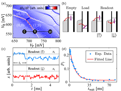
Figure 1: (a) Charge stability diagram of the DQD measured by differentiating the single-electron transistor (SET) current $(I_{S})$ as a function of the $V_{B}$ and $V_{P}$ gate voltages. The pulse sequence for measuring the spin relaxation time ($T_{1}$) via the (0,0)-(1,0) charge transition line is overlaid on the data. (b) Illustration of the energy states of the pulse sequence: the measurement starts with emptying the electron in the QD at point E, then injecting a random spin into it and waiting for a time at point W, finally moving to point R for STC conversion. (c) The readout traces ($x$) are achieved by amplifying $I_{S}$ with a room temperature low noise current amplifier (DLCPA - 200) and a JFET preamplifier (SIM910), and then low-pass filtering the amplified signal using an analog filter (SIM965) with a bandwidth of 10 kHz. The blue and red curves represent spin up ($\ket{\uparrow}$) and spin down ($\ket{\downarrow}$) traces at point R, respectively. By comparing the maximum of each readout traces ($x_{\rm max}$) with the threshold voltage ($x_{\rm t}$) within the readout time ($t_{\rm r}$), we can distinguish the different spin states. (d) A typical exponential decay of spin-up probability with 1000 repeated measurements for each point. The exponential fit for $1/T_{1}$ is $112\pm 6$ s^-1

.

The readout traces we measured by amplifying the single-electron transistor (SET) current ($I_{S}$) with a room temperature low noise current amplifier (DLCPA - 200) and a JFET preamplifier (SIM910) and then low-pass filtering the amplified signal using an analog filter (SIM965) with a bandwidth of 10 kHz. The blue and red curve represent spin up and spin down traces measured at point R, respectively. By comparing the maximum value of each readout traces with the threshold voltage within the readout time, we can distinguish the different spin states.

The state-to-charge (STC) conversion is realized by distinguishing two different traces in the readout phase, as shown in Fig. 1(c). Single electron tunneling onto or off the QD causes a change in the readout trace $x$. We distinguish the different spin states in the QD by comparing readout trace $x$ with the threshold voltage $x_{\rm t}$. If $x$ remains below the threshold during the readout phase, we assume it is a $\ket{\downarrow}$ state and vice versa. Then, we emptied QDs by raising the electrochemical potential and waiting for enough time. After the empty stage, we loaded a new electron with a random spin state and waited for the next readout stage.

We measured the electron spin relaxation time by repeating this three-stage pulse and changing the waiting time in the loading stage. Fig. 1(d) shows typical exponential decay of the measured spin-up probability $P^{M}_{\uparrow}=\rho\cdot e^{-t/T_{1}}+\alpha$, where $\rho$ is the amplitude and $\alpha$ is the dark count. Additionally, we can manipulate the spin qubit by using a similar pulse and a microwave pulse, as reported in Ref. [35].

2.2 The readout visibility

We demonstrated a maximum visibility $V^{R}=85.4\%$ while measuring the spin relaxation time as shown in Fig. 2(a). $V^{R}=F_{\uparrow}^{R}+F_{\downarrow}^{R}-1$ is calculated from the simulated data via the Monte-Carlo method. $F_{\downarrow}^{R}$ and $F_{\uparrow}^{R}$ are the readout fidelities of $\ket{\downarrow}$ and $\ket{\uparrow}$. In Fig. 2(b), we simulated the distribution of the single-shot signal with a high accuracy (R squared $\approx 0.98$) of the corresponding fitting process (the right inset in Fig 2.(b)). The insets in Fig 2.(b) shows the fitting results of the averaged readout traces ($\bar{x}$) and the probability density function (PDF) of the traces maximum ($x_{\rm max}$) of the readout phase for every single measurement. The details about the simulation process and the insets in Fig. 2(b) are discussed in Sec. 1 of the Supplementary Materials [23, 27, 30, 31, 32]. By fitting $\bar{x}$ with the rate equations, we obtained the tunneling rates of the state-to-charge conversion as shown in the left inset of Fig. 2(b): $\Gamma_{\uparrow}^{\rm out}=6.0\pm 0.1\ {\rm kHz}$, $\Gamma_{\downarrow}^{\rm out}=27\pm 2\ {\rm Hz}$ and $\Gamma_{\downarrow}^{\rm in}=1.39\pm 0.04\ {\rm kHz}$.

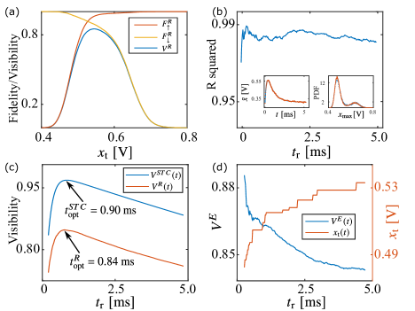
Figure 2: (a) The fidelities of spin-up and spin-down state ($F_{\uparrow}^{R},F_{\downarrow}^{R}$) and the related readout visibility ($V^{R}$) versus $x_{\rm t}$. (b) The fitting model for the distribution of the experimental data has a high value of R squared ($\approx 0.98$), which indicates good accuracy of the results. The insets show fitting results for the averaged traces ($\bar{x}$) and the probability density function (PDF) of the maximum value of each readout traces ($x_{\rm max}$). (c) The state-to-charge (STC) conversion visibility ($V^{STC}$) versus $t_{\rm r}$ and the corresponding maximum value $V^{R}$. $t_{\rm opt}^{R}$ (the bottom arrow) and $t_{\rm opt}^{STC}$ (the top arrow) are not equal. (d) The electrical detection visibility ($V^{E}$) and the corresponding optimal threshold voltage $x_{\rm t}$ as a function of readout time $t_{\rm r}$.

In the traditional methods, state-to-charge conversion visibility ($V^{STC}$) and electrical detection visibility ($V^{E}$) need to be optimized to obtain a high readout visibility $V^{R}$. Instead, the threshold-independent single-shot readout method does not need to perform such a cumbersome operation. Here we introduce the steps of this novel method. First, we calculated $V^{STC}$ as a single peaked function of readout time $t_{\rm r}$ with the knowledge of tunneling rates as shown in Fig. 2(c). (We will describe the details of this part in Sec. 2 of the Supplementary Materials.) For exceeding 99% $V^{STC}$, three criteria are given in Ref. [30], including $E_{z}/T_{\rm e}>13$, $T_{1}*\Gamma^{\rm out}_{\uparrow}>100$ and $\Gamma_{\rm s}/\Gamma^{\rm in}_{\downarrow}>12$. Here, we have $\Gamma_{\rm s}=50$ kHz, $B_{\rm ext}=1.5$ T and $T_{\rm e}=180.5\pm 8.1$ mK as mentioned in Ref. [34]; thus, the disagreement of the condition $E_{z}/T_{\rm e}=11.22<13$ limits the maximum $V^{STC}$ to 97.15%. Fig. 2(c) also shows the readout visibility $V^{R}$ as a single peaked function of $t_{\rm r}$ (details are discussed in Sec. 4 of the Supplementary Materials). However, the optimal readout time $t_{\rm opt}$ for $V^{STC}$ is different from that for $V^{R}$. Thus, to obtain the maximum $V^{R}$, we should consider the readout time $t_{\rm r}$ and threshold voltage $x_{\rm t}$ together.

Due to the lack of a simple analytical expression for the distribution of $x_{\rm max}$, $V^{E}$ cannot be obtained directly. Here, we obtain $V^{E}$ by factorizing $V^{R}$ into $V^{STC}=F_{\uparrow}^{STC}+F_{\downarrow}^{STC}-1$ and $V^{E}=F_{\uparrow}^{E}+F_{\downarrow}^{E}-1$, as the following formula shows:

$$V^{R}=F_{\uparrow}^{R}+F_{\downarrow}^{R}-1=V^{STC}\times V^{E}.$$ (1)

Here, readout fidelities $F_{\downarrow}^{R}$ and $F_{\uparrow}^{R}$ are shown the following:

$$F_{\downarrow}^{R} =F_{\downarrow}^{STC}F_{\downarrow}^{E}+(1-F_{\downarrow}^{STC})(1-F_{\uparrow}^{E}),$$

$$F_{\uparrow}^{R} =F_{\uparrow}^{STC}F_{\uparrow}^{E}+(1-F_{\uparrow}^{STC})(1-F_{\downarrow}^{E}),$$ (2)

$t_{\rm r}$, the corresponding readout visibility $V^{R}$ is obtained from the Monte-Carlo method and the state-to-charge visibility $V^{STC}$ is calculated as above. Thus, we have the electrical detection visibility $V^{E}=V^{R}/V^{STC}$ indirectly. Fig. 2(d) shows the maximum $V^{E}$ and the corresponding optimal threshold voltage $x_{\rm t}$ versus readout time $t_{\rm r}$. Considering the increasing or constant nature of the maximum value $x_{\rm t}$ as $t_{\rm r}$ increases in each readout trace, it can be inferred that the optimal threshold voltage $x_{\rm t}$ follows a monotonically non-decreasing pattern. On the other hand, the longer $t_{\rm r}$ we consider, the more noise is added to the trace. Therefore, it is obvious that $V^{E}$ will decrease as $t_{\rm r}$ increases.

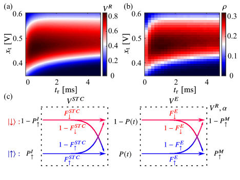
Figure 3: (a)(b) $V^{R}$ and the amplitude ($\rho$) as a function of $t_{\rm r}$ and $x_{\rm t}$, showing the consistency in scaled color image. (c) The qubits are prepared in $\ket{\uparrow}$ with probability $P^{I}_{\uparrow}$. Throughout the STC conversion ($F_{\uparrow}^{STC}$, $F_{\downarrow}^{STC}$), the electron tunnels out from QD with probability $P(t)$. Similarly, the electrons are measured as $\ket{\uparrow}$ with $P_{\uparrow}^{M}$ throughout the electrical detection process ($F_{\uparrow}^{E}$, $F_{\downarrow}^{E}$).

2.3 Relation between $P^{M}_{\uparrow}$, $P^{I}_{\uparrow}$ and $V^{R}$

Now, we focus on the details of readout visibility $V^{R}$. First, we exhibit the relationship between $V^{R}$ and readout time $t_{\rm r}$ along with threshold voltage $x_{\rm t}$ via the Monte-Carlo method in Fig. 3(a). As mentioned in Sec.2.2, $x_{\rm t}$ corresponding to the maximum electrical detection visibility $V^{E}$ increases as $t_{\rm r}$ increases. The state-to-charge visibility $V^{STC}$ is a uni-modal function of $t_{\rm r}$. Therefore, $V^{R}$ increases first and then decreases along the $t_{\rm r}$ axis, and $x_{\rm t}$ of the maximum $V^{R}$ increases along the $x_{\rm t}$ axis as $t_{\rm r}$ increases.

Then, we drew the spin up probability $\rho$ in the same range in Fig. 3(b) for comparison. The expression $\rho=P^{M}_{\uparrow}|_{t_{\rm wait}\to 0}-\alpha$ is obtained by fitting the experimental data of the spin relaxation process with an exponential function $P^{M}_{\uparrow}=\rho\cdot e^{-t/T_{1}}+\alpha$. Here, $\alpha=P^{M}_{\uparrow}|_{t_{\rm wait}\to+\infty}$ is the dark count of the spin relaxation process. Fig. 3(a) and (b) shows that the readout visibility $V^{R}$ and probability $\rho$ are consistent in the scaled color images.

To analyze this consistency, we focus on the details of Eq.1. As shown in Fig. 3(c), we note the spin-up probability at the beginning of the readout phase as the prepared probability $P^{I}_{\uparrow}$. Throughout the STC conversion, the probability of the tunneling events detected within readout time $t_{\rm r}$ ($P(t)$) depends on the condition probability that electrons in $\ket{\uparrow}$ ($F_{\uparrow}^{STC}$) or $\ket{\downarrow}$ ($1-F_{\downarrow}^{STC}$) tunnel out:

$$P(t)=F_{\uparrow}^{STC}P^{I}_{\uparrow}+(1-F_{\downarrow}^{STC})(1-P^{I}_{\uparrow}).$$ (3)

Similarly, by comparing the maximum of each readout traces $x_{\rm max}$ with threshold voltage $x_{\rm t}$, the electron is measured with $P^{M}_{\uparrow}$ throughout the electrical detection ($F_{\uparrow}^{E}$, $F_{\downarrow}^{E}$):

$$P^{M}_{\uparrow} =P(t)F_{\uparrow}^{E}+(1-P(t))(1-F_{\downarrow}^{E}).$$ (4)

We factorized Eq. 4 into sectors with and without $P^{I}_{\uparrow}$ and substituted Eq. 2 into Eq. 4 to obtain the expression of $\alpha$: $\alpha=1-F_{\downarrow}^{R}$. Then, the relation between the measured probability $P^{M}_{\uparrow}$, prepared probability $P^{I}_{\uparrow}$ and readout visibility $V^{R}$ can be extracted by substituting Eq. 1 into Eq. 4:

$$P^{M}_{\uparrow}=P^{I}_{\uparrow}\times V^{R}+\alpha.$$ (5)

The details of derivation are discussed in Sec. 6 of the Supplementary Materials.

Eq. 5 reveals that the measured probability $P^{M}_{\uparrow}$ linearly depends on the readout visibility $V^{R}$ and dark count $\alpha$. Here, the slope is the prepared probability $P^{I}_{\uparrow}$ and the intercept is the dark count. By substituting Eq. 5 into the definition of the probability $\rho=P^{M}_{\uparrow}|_{t_{\rm wait}\to 0}-\alpha$, we got $\rho=P^{I}_{\uparrow}|_{t_{\rm wait}\to 0}\times V^{R}$. Since $P^{I}_{\uparrow}$ only depends on the ”Wait” process, the probability $\rho$ is proportional to the readout visibility $V^{R}$ in the readout process, and this proportional relation between $\rho$ and $V^{R}$ explains their consistency in the scaled color images shown in Fig. 3(a) and (b). Since $P^{I}_{\uparrow}$ only depends on the ”Wait” process, we try to apply the threshold-independent data process methods in Sec.2.4.

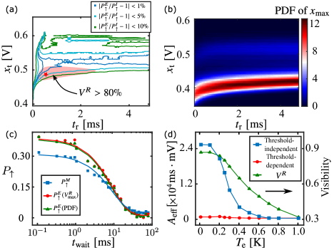
Figure 4: (a) The bias of the expected probability ($P_{\uparrow}^{E}$) relative to $P^{I}_{\uparrow}$ ($P_{\uparrow}^{E}/P^{I}_{\uparrow}-1$) as a function of readout time $t_{\rm r}$ and threshold voltage $x_{\rm t}$. The regions between the blue, cyan and green curves represent $A_{\rm eff}$ where $|P_{\uparrow}^{E}/P^{I}_{\uparrow}-1|<1\%$, $5\%$ and $10\%$, respectively. For comparison, the red star represents the position of the maximum readout visibility $V^{R}_{\rm max}$, and the points in the pink shadow region satisfy $V^{R}>80\%$. (b)The map of PDF of $x_{\rm max}$ (maximum of the readout trace). The monotonically non-decreasing feature of the maximum function causes the positions of the two peaks to increase as $t_{\rm r}$ increases. The outline of the valley between two peaks is similar to that of (a). (c) The extrapolated probability $P_{\uparrow}^{E}$ figured out from the threshold-independent methods at $V^{R}_{\rm max}$ (red circles) and minimum between two peaks in PDF of $x_{\rm max}$ (green triangles). The measured probabilities $P_{\uparrow}^{M}$ (blue rectangles) are obtained from the exponential decay process at $V^{R}_{\rm max}$ directly. The solid curves with the same color illustrate the corresponding exponential fitting results. $t_{\rm wait}$ is logarithmic, showing that the threshold-independent method suppresses dark count $\alpha$ and improves probability $\rho$. (d) The left y-axis shows that $A_{\rm eff}$ is a function of the electron temperature $T_{\rm e}$ in both threshold-independent method and threshold-dependent readout. The right y-axis shows the corresponding readout visibility $V^{R}$. When $T_{\rm e}$ exceeds 100 mK, $V^{R}$ and $A_{\rm eff}$ of the threshold-independent methods will decrease as $T_{\rm e}$ increases. The $A_{\rm eff}$ of the threshold-independent method is higher than that of the threshold-dependent method until $T_{\rm e}=0.7$ K as $V^{R}$ fixed at 0.5.

2.4 Threshold-independent data process

We calculate the extrapolated probability ($P^{E}_{\uparrow}$) for each $t_{\rm r}$ and $x_{\rm t}$ by applying Eq. 5 directly:

$$P^{E}_{\uparrow}=(P^{M}_{\uparrow}-\alpha)/V^{R}.$$ (6)

Here, $P^{E}_{\uparrow}$ is the extrapolated probability and can be calculated from by $V^{R}$ and $\alpha$. Since $P^{I}_{\uparrow}$ is independent of the threshold voltage $x_{\rm t}$ and readout time $t_{\rm r}$, we speculated that the extrapolated probability $P^{E}_{\uparrow}$ is threshold independent as well with no constraints on $x_{\rm t}$ and $t_{\rm r}$. We calculate the contour map of $|P^{E}_{\uparrow}/P^{I}_{\uparrow}-1|$, as shown in Fig. 4(a). The region inside the blue, cyan and green curves represent the area where $|P_{\uparrow}^{E}/P^{I}_{\uparrow}-1|<1\%$, $5\%$ and $10\%$, respectively. We compared the regions with the visibility $V^{R}$ map in Fig. 4(a). The pink shadow represents where $V^{R}>80\%$, and the red star represents the position of $V^{R}_{\rm max}$. There is a discrepancy between $|P^{E}_{\uparrow}/P^{I}_{\uparrow}-1|$ and the $V^{R}$ map, revealing that the optimal $x_{\rm t}$ and $t_{\rm r}$ for the readout visibility $V^{R}$ are not optimal for $P^{E}_{\uparrow}$.

In Sec.5 of the Supplementary Materials, we will use the simulated traces to illustrate that the region $|P_{\uparrow}^{E}/P^{I}_{\uparrow}-1|<1\%$ almost covers the whole considered region under ideal circumstances. We calculated the cumulative error (CE) and absolute value of error between the distribution of experimental and simulated traces as a function of threshold voltage $x_{\rm t}$. The shape of the CE curve demonstrates that the error in the fitting process comes from the bin edges. The features of the bin edge error are shown in the contour map of $|P^{E}_{\uparrow}/P^{I}_{\uparrow}-1|$ in Fig. 2(b) and (c) in the Supplementary Materials.

In the valley region between the two peaks, errors from bin edges are minimal, as shown in the map of the distribution of $x_{\rm max}$ in Fig. 4(a). The outline of the valley region in Fig. 4(b) resembles that of $|P^{E}_{\uparrow}/P^{I}_{\uparrow}-1|<1\%$ and 5$\%$ in Fig. 4(a). As a compromise method, we can choose $x_{\rm t}$ around the minimum between two peaks of the distribution of $x_{\rm max}$ instead of $x_{\rm t}$ at $V^{R}_{\rm max}$.

By using the threshold-independent method to processing the experimental data, we calculated the extrapolated probability $P^{E}_{\uparrow}$ $t_{\rm r}$ and threshold voltage $x_{\rm t}$ at $V^{R}_{\rm max}$ ($P^{E}_{\uparrow}(V^{R}_{\rm max})$), along with the minimum between two peaks in PDF of the maximum of each readout trace $x_{\rm max}$ with the same $t_{\rm r}$ ($P^{E}_{\uparrow}({\rm PDF})$). Fig. 4(c) shows $P^{E}_{\uparrow}$ as a function of waiting time of the spin decaying process $t_{\rm wait}$, and we plot measured probability $P^{M}_{\uparrow}$ for comparison. The results demonstrate that the threshold-independent method suppresses dark count $\alpha$ and increases probability $\rho=P^{M}_{\uparrow}|_{t_{\rm wait}\to 0}-\alpha$, and $P^{E}_{\uparrow}({\rm PDF})$ calculated via the compromise method is slightly different from $P^{E}_{\uparrow}(V^{R}_{\rm max})$. $x_{\rm t}$ and readout time $t_{\rm r}$ in a wider range with only a $1\%$ loss of accuracy.

Finally, we tried to use the area where $|P^{E}_{\uparrow}/P^{I}_{\uparrow}-1|<1\%$ as $A_{\rm eff}$ to quantify the accuracy and efficiency of different data processing methods. For comparison, we use the area of where $|P^{M}_{\uparrow}/P^{I}_{\uparrow}-1|<1\%$ as $A_{\rm eff}$ for the commonly used threshold-dependent method. The $A_{\rm eff}$ of the threshold-independent method is 60 times larger than that of the threshold-dependent method, meaning that we can choose threshold voltage $x_{\rm t}$ and readout time $t_{\rm r}$ in a 60 times larger range and maintain 99$\%$ accuracy. In addition, the threshold-independent method is more robust and can calibrate the measured result from the interference of the experimental hardware limitation.

2.5 Influence of the Electron Temperature

Furthermore, we try to characterize the influence of $T_{\rm e}$. Ref. [30] assumes that the tunneling rate follows a Fermi distribution:

$$\Gamma^{\rm out}_{\uparrow,\ \downarrow}= [1-f(\epsilon\pm E_{z}/2,\ T_{\rm e})]\Gamma^{\rm out},$$

$$\Gamma^{\rm in}_{\uparrow,\ \downarrow}= f(\epsilon\pm E_{z}/2,\ T_{\rm e})\Gamma^{\rm in},$$ (7)

where $f(\epsilon\pm E_{z}/2,\ T_{\rm e})$ is the Fermi-Dirac function with $-$ for $\ket{\downarrow}$ and $+$ for $\ket{\uparrow}$, $\Gamma^{\rm out}(\Gamma^{\rm in})$ is the maximum tunnel out(in) rate, $\Gamma^{\rm out}_{\uparrow,\ \downarrow}(\Gamma^{\rm in}_{\uparrow,\ \downarrow})$ are tunneling rates of corresponding spin state, and $\epsilon$ is the energy splitting between the Fermi energy of the electron reservoir and the average energy of $\ket{\uparrow}$ and $\ket{\downarrow}$ electrons in QD. Therefore, $\epsilon+E_{z}/2$($\epsilon-E_{z}/2$) represents the energy splitting between the Fermi energy of the electron reservoir and the energy state of $\ket{\uparrow}$($\ket{\downarrow}$) electron in QD.

By defining $R_{G}=\Gamma_{\uparrow}^{\rm out}/\Gamma_{\downarrow}^{\rm out}$, $\epsilon$ can be obtained as follows:

$$\epsilon=-k_{B}T_{\rm e}{\rm ln}\left(\frac{1-R_{G}}{R_{G}}\frac{1}{e^{\frac{-E_{z}}{2k_{B}T_{\rm e}}}-e^{\frac{E_{z}}{2k_{B}T_{\rm e}}}}\right).$$ (8)

We [extracted] the maximum tunneling rates $\Gamma^{\rm out}$ and $\Gamma^{\rm in}$ by substituting $\epsilon$ into Eq. 7.

Then, we tried to simulate the single-shot readout process at different electron temperature $T_{\rm e}$. Assuming that tunneling rates $\Gamma^{\rm out}$ and $\Gamma^{\rm in}$ are not associated with $T_{\rm e}$, we directly substituted $T_{\rm e}$ into Eq. 7 to calculate the tunneling rates. We used the Monte-Carlo method to generate the simulated traces with a fixed external magnetic field $B_{\rm ext}=1.5$ T at different $T_{\rm e}$. The left y-axis in Fig. 4(d) shows the $A_{\rm eff}$ of [both] the threshold-independent method and the threshold-dependent method at different $T_{\rm e}$. The right y-axis shows the corresponding readout visibility $V^{R}$. The simulation results exhibit that the $A_{\rm eff}$ of the threshold-independent methods is 60 times greater than that of the threshold-dependent method when $T_{\rm e}<0.1$ K. As $T_{\rm e}$ increases, $A_{\rm eff}$ of the threshold-independent methods decreases. It is larger than that of the threshold-dependent method until $T_{\rm e}=0.7$ K. When $T_{\rm e}>0.7$ K, the corresponding $V^{R}<0.5$. Here, we [can] give the boundary condition of the threshold-independent method as $T_{\rm e}=0.7$ K when $B_{\rm ext}=1.5$ T.

3 Summary

We described a threshold-independent method of the single-shot readout data process based on the linear dependence of measured probability $P_{\uparrow}^{M}$ with the corresponding readout visibility $V^{R}$ and dark count $\alpha$. Due to the error during the fitting process from bin edges, the extrapolated probability deviates from the prepared probability. For compromise, the region of readout time $t_{\rm r}$ and threshold voltage $x_{\rm t}$ are reduced to the minimum of the distribution of the maximum of each readout trace $x_{\rm max}$ to ensure that the accuracy loss of extrapolated probability $P_{\uparrow}^{E}$ is less than $1\%$. Then, we used $A_{\rm eff}$ to quantify the efficiency of the threshold-independent method and the threshold-dependent readout. The result shows that the $A_{\rm eff}$ of the threshold-independent method is more than 60 times larger that of the threshold-dependent method. Moreover, we simulated the single-shot readout process at different electron temperature $T_{\rm e}$. We broaden the boundary condition of the single-shot readout to 0.7 K with $B_{\rm ext}=1.5$ T, where $V^{R}=0.5$. The significance of employing the threshold-independent method will progressively increase as the experiment advances towards the fault tolerance threshold of the logic qubit, particularly when operating under high electron temperature conditions [36, 37, 38].

References

- [1] Juha T. Muhonen, Juan P. Dehollain, Arne Laucht, et al. Storing quantum information for 30 seconds in a nanoelectronic device. Nature Nanotechnology, 9:986, 2014.
- [2] Xin Zhang, Hai-Ou Li, Gang Cao, et al. Semiconductor quantum computation. National Science Review, 6:32, 2019.
- [3] J. P. Dodson, Nathan Holman, Brandur Thorgrimsson, et al. Fabrication process and failure analysis for robust quantum dots in silicon. Nanotechnology, 31:505001, 2020.
- [4] Ruoyu Li, Luca Petit, David P. Franke, et al. A crossbar network for silicon quantum dot qubits. Science Advances, 4:eaar3960, 2018.
- [5] Leon C Camenzind, Simon Geyer, Andreas Fuhrer, et al. A spin qubit in a fin field-effect transistor. arXiv preprint, 2103:07369, 2021.
- [6] A. M. J. Zwerver, T. Krähenmann, T. F. Watson, et al. Qubits made by advanced semiconductor manufacturing. Nature Electronics, 5:184, 2022.
- [7] J. Yoneda, K. Takeda, T. Otsuka, et al. A quantum-dot spin qubit with coherence limited by charge noise and fidelity higher than 99.9%. Nature Nanotechnology, 13:102, 2018.
- [8] K. W. Chan, W. Huang, C. H. Yang, et al. Assessment of a silicon quantum dot spin qubit environment via noise spectroscopy. Phys. Rev. Applied, 10:044017, 2018.
- [9] Xiao Xue, Maximilian Russ, Nodar Samkharadze, et al. Quantum logic with spin qubits crossing the surface code threshold. Nature, 601:343, 2022.
- [10] Akito Noiri, Kenta Takeda, Takashi Nakajima, et al. Fast universal quantum gate above the fault-tolerance threshold in silicon. Nature, 601:338, 2022.
- [11] Adam R. Mills, Charles R. Guinn, Michael J. Gullans, et al. Two-qubit silicon quantum processor with operation fidelity exceeding 99%. Science Advances, 8:eabn5130, 2022.
- [12] JM Elzerman, R Hanson, LH Willems van Beveren, et al. Single-shot read-out of an individual electron spin in a quantum dot. Nature, 430:431, 2004.
- [13] D. M Zajac, T. M Hazard, X. Mi, E. Nielsen, and J. R Petta. Scalable gate architecture for a one-dimensional array of semiconductor spin qubits. Physical Review Applied, 6(5), 2016.
- [14] P. Pakkiam, A. V. Timofeev, M. G. House, et al. Single-shot single-gate rf spin readout in silicon. Phys. Rev. X, 8:041032, 2018.
- [15] Anderson West, Bas Hensen, Alexis Jouan, et al. Gate-based single-shot readout of spins in silicon. Nature Nanotechnology, 14:437, 2019.
- [16] Guoji Zheng, Nodar Samkharadze, Marc L. Noordam, et al. Rapid gate-based spin read-out in silicon using an on-chip resonator. Nature Nanotechnology, 14:742, 2019.
- [17] J. R. Prance, B. J. Van Bael, C. B. Simmons, et al. Identifying single electron charge sensor events using wavelet edge detection. Nanotechnology, 26:215201, 2015.
- [18] K. C. Nowack, M. Shafiei, M. Laforest, et al. Single-shot correlations and two-qubit gate of solid-state spins. Science, 333:1269, 2011.
- [19] B. D’Anjou and W. A. Coish. Optimal post-processing for a generic single-shot qubit readout. Phys. Rev. A, 89:012313, 2014.
- [20] Tom Struck, Javed Lindner, Arne Hollmann, et al. Robust and fast post-processing of single-shot spin qubit detection events with a neural network. Scientific Reports, 11(1):16203, 2021.
- [21] S. K. Gorman, Y. He, M. G. House, et al. Tunneling statistics for analysis of spin-readout fidelity. Phys. Rev. Applied, 8:034019, 2017.
- [22] Raisei Mizokuchi, Masahiro Tadokoro, and Tetsuo Kodera. Detection of tunneling events in physically defined silicon quantum dot using single-shot measurements improved by numerical treatments. Applied Physics Express, 13(12):121004, nov 2020.
- [23] Andrea Morello, Jarryd J. Pla, Floris A. Zwanenburg, et al. Single-shot readout of an electron spin in silicon. Nature, 467:687, 2010.
- [24] M. Veldhorst, J. C. C. Hwang, C. H. Yang, et al. An addressable quantum dot qubit with fault-tolerant control-fidelity. Nature Nanotechnology, 9:981, 2014.
- [25] E. Kawakami, P. Scarlino, D. R. Ward, et al. Electrical control of a long-lived spin qubit in a Si/SiGe quantum dot. Nature Nanotechnology, 9:666, 2014.
- [26] Lada Vukušić, Josip Kukučka, Hannes Watzinger, et al. Single-shot readout of hole spins in Ge. Nano Letters, 18:7141, 2018.
- [27] H. Büch, S. Mahapatra, R. Rahman, et al. Spin readout and addressability of phosphorus-donor clusters in silicon. Nature Communications, 4:2017, 2013.
- [28] Lucio Robledo, Lilian Childress, Hannes Bernien, et al. High-fidelity projective read-out of a solid-state spin quantum register. Nature, 477:574, 2011.
- [29] A. R. Mills, C. R. Guinn, M. M. Feldman, et al. High fidelity state preparation, quantum control, and readout of an isotopicallyenriched silicon spin qubit. arXiv preprint, 2204:09551, 2022.
- [30] D Keith, SK Gorman, L Kranz, et al. Benchmarking high fidelity single-shot readout of semiconductor qubits. New Journal of Physics, 21:063011, 2019.
- [31] Ming Xiao, MG House, and Hong Wen Jiang. Measurement of the spin relaxation time of single electrons in a silicon metal-oxide-semiconductor-based quantum dot. Phys. Rev. Lett., 104:096801, 2010.
- [32] L. A. Tracy, T. M. Lu, N. C. Bishop, et al. Electron spin lifetime of a single antimony donor in silicon. Applied Physics Letters, 103:143115, 2013.
- [33] M. G. House, Ming Xiao, GuoPing Guo, et al. Detection and measurement of spin-dependent dynamics in random telegraph signals. Phys. Rev. Lett., 111:126803, 2013.
- [34] Xin Zhang, Rui-Zi Hu, Hai-Ou Li, et al. Giant anisotropy of spin relaxation and spin-valley mixing in a silicon quantum dot. Phys. Rev. Lett., 124:257701, 2020.
- [35] Rui-Zi Hu, Rong-Long Ma, Ming Ni, et al. An operation guide of Si-MOS quantum dots for spin qubits. Nanomaterials, 11:2486, 2021.
- [36] W. Huang, C. H. Yang, K. W. Chan, et al. Fidelity benchmarks for two-qubit gates in silicon. Nature, 569:532, 2019.
- [37] L. Petit, H. G. J. Eenink, M. Russ, et al. Universal quantum logic in hot silicon qubits. Nature, 580:355, 2020.
- [38] Kenta Takeda, Akito Noiri, Takashi Nakajima, et al. Quantum tomography of an entangled three-qubit state in silicon. Nature Nanotechnology, 16:965, 2021.