Alternately Optimized Graph Neural Networks

Abstract

Graph Neural Networks (GNNs) have greatly advanced the semi-supervised node classification task on graphs. The majority of existing GNNs are trained in an end-to-end manner that can be viewed as tackling a bi-level optimization problem. This process is often inefficient in computation and memory usage. In this work, we propose a new optimization framework for semi-supervised learning on graphs from a multi-view learning perspective. The proposed framework can be conveniently solved by the alternating optimization algorithms, resulting in significantly improved efficiency. Extensive experiments demonstrate that the proposed method can achieve comparable or better performance with state-of-the-art baselines while it has significantly better computation and memory efficiency.

1 Introduction

Graph is a fundamental data structure that denotes pairwise relationships between entities in a wide variety of domains (Wu et al., 2019b; Ma & Tang, 2021). Semi-supervised node classification is one of the most crucial tasks on graphs. Given graph structure, node features, and a part of labels, the task aims to predict labels of the unlabeled nodes. In recent years, Graph Neural Networks (GNNs) have been proven to be powerful in semi-supervised node classification (Gilmer et al., 2017; Kipf & Welling, 2016; Veličković et al., 2017). A typical GNN model mainly contains two operators, i.e., feature transformation and feature propagation. The feature transformation operator encodes input features into a low dimensional space, which is typically a learnable function. The feature propagation operator exploits graph structure to propagate information to its neighbors, which usually follows the message passing scheme  (Gilmer et al., 2017).

While the message passing scheme (Gilmer et al., 2017) empowers GNNs with the superior capability of capturing both node features and graph structure information, they suffer from the scalability limitation when training the GNNs in an end-to-end way (Hamilton et al., 2017). The end-to-end training of GNNs are in fact inefficient in computation cost and memory usage. In the forward computation, features will be propagated through all propagation layers in every epoch. In the backward computation, the gradients need be back-propagated through all propagation layers. In addition, every propagation layer needs to maintain all the hidden states for back-propagation, leading to a high memory cost.

There are extensive efforts trying to improve the scalability and efficiency of GNNs, including pre-computing methods (Wu et al., 2019a; Rossi et al., 2020), post-computing methods(Huang et al., 2020), sampling methods (Hamilton et al., 2017; Chen et al., 2018), and distributed methods (Chiang et al., 2019; Shao et al., 2022). In particular, pre-computing and post-computing methods are the most efficient ones in dealing with large-scale graphs. SGC (Wu et al., 2019a) and SIGN (Rossi et al., 2020) first propagate features as a pre-processing and then an MLP is trained based on the propagated features. C&S (Huang et al., 2020) first trains an encoder on node features and then applies correction and smoothing steps. These methods only need to propagate information once during the whole training process so they are highly scalable and efficient. However, the performance of these GNNs is often worse than the end-to-end GNNs that propagate features in every epoch, such as APPNP, especially when the labeling rate is small (Duan et al., 2022; Palowitch et al., 2022).

In this paper, we first demonstrate that the majority of aforementioned GNNs for node classification can be considered as solving a bi-level optimization problem. Instead of following the above perspective as previous GNNs, we propose a single-level optimization problem to couple the node features and graph structure information through a multi-view semi-supervised learning framework. This new optimization problem can be conveniently optimized in an alternating way, leading to the proposed algorithm ALT-OPT. Extensive experiments demonstrate that ALT-OPT not only remarkably alleviates the computational and memory inefficiency issues of end-to-end trainable GNNs but also achieves comparable or even better performance than the state-of-the-art GNNs.

2 GNNs as Bi-level Optimization

Notations. We use bold upper-case letters such as $\mathbf{X}$ to denote matrices. $\mathbf{X}_{i}$ denotes its $i$-th row and ${\mathbf{X}}_{ij}$ indicates the $i$-th row and $j$-th column element. We use bold lower-case letters such as $\mathbf{x}$ to denote vectors. The Frobenius norm and trace of a matrix $\mathbf{X}$ are defined as $\|\mathbf{X}\|_{F}=\sqrt{\sum_{ij}\mathbf{X}_{ij}^{2}}$ and $tr(\mathbf{X})=\sum_{i}\mathbf{X}_{ii}$. Let $\mathcal{G}=(\mathcal{V},\mathcal{E})$ be a graph, where $\mathcal{V}$ is the node set and $\mathcal{E}$ is the edge set. $\mathcal{N}_{i}$ denotes the neighborhood node set for node $v_{i}$. The graph can be represented by an adjacency matrix $\mathbf{A}\in\mathbb{R}^{n\times n}$, where $\mathbf{A}_{ij}>0$ indices that there exists an edge between nodes $v_{i}$ and $v_{j}$ in $\mathcal{G}$, or otherwise $\mathbf{A}_{ij}=0$. Let ${\mathbf{D}}=diag(d_{1},d_{2},\dots,d_{n})$ be the degree matrix, where $d_{i}=\sum_{j}\mathbf{A}_{ij}$ is the degree of node $v_{i}$. The graph Laplacian matrix is defined as $\mathbf{L}=\mathbf{D}-\mathbf{A}$. We define the normalized adjacency matrix as ${\tilde{{\mathbf{A}}}}={\mathbf{D}}^{-\frac{1}{2}}{\mathbf{A}}{\mathbf{D}}^{-\frac{1}{2}}$ and the normalized Laplacian matrix as ${\tilde{{\mathbf{L}}}}={\mathbf{I}}-{\tilde{{\mathbf{A}}}}$. Furthermore, suppose that each node is associated with a $d$-dimensional feature $\mathbf{x}$ and we use $\mathbf{X}=[\mathbf{x}_{1},\dots,\mathbf{x}_{n}]^{\top}\in\mathrm{R}^{n\times d}$ to denote the feature matrix. In this work, we focus on the node classification task on graphs. Given a graph $\mathcal{G}=\{\mathbf{A},\mathbf{X}\}$ and a partial set of labels $\mathcal{Y}_{L}=\{\mathbf{y}_{1},\dots,\mathbf{y}_{l}\}$ for node set ${\mathcal{V}}_{L}=\{v_{1},\dots,v_{l}\}$, where $\mathbf{y}_{i}\in\mathbb{R}^{c}$ is a one-hot vector with $c$ classes, our goal is to predict labels of unlabeled nodes. Labels of graph $\mathcal{G}$ can be represented as a label matrix $\mathbf{Y}\in\mathbb{R}^{n\times c}$, where $\mathbf{Y}_{i}=\mathbf{y}_{i}$ if $v_{i}\in{\mathcal{V}}_{L}$ and $\mathbf{Y}_{i}=\mathbf{0}$ if $v_{i}\in{\mathcal{V}}_{U}$ where ${\mathcal{V}}_{U}={\mathcal{V}}\setminus{\mathcal{V}}_{L}$.

There are some recent works  (Zhu et al., 2021; Ma et al., 2021; Yang et al., 2021) that have unified GNNs into an optimization framework. For example, it has been proven that the message passing of GNNs, such as GCN, GAT, PPNP, and APPNP, can be considered as optimizing graph signal denoising problems (Ma et al., 2021). Considering the GNNs for node classification tasks, there are mainly two steps: (1) Forward process that fuses both features and structure information into a low-dimensional representation; and (2) Backward process that trains the whole model through gradient backpropagation. Aforementioned optimization perspectives (Zhu et al., 2021; Ma et al., 2021; Yang et al., 2021) only consider the forward computation of GNNs. In this work, we highlight that many existing works can be understood and unified as a bi-level optimization problem when considering both forward and backward processes:

$$\begin{aligned} &~{}~{}~{}~{}~{}~{}~{}~{}\min_{\Theta,\Phi}\|f_{\Theta}({\mathbf{F}}_{L})-{\mathbf{Y}}_{L}\|_{F}^{2},\\ \text{s.t.}\quad{\mathbf{F}}=&\operatorname*{arg\,min}_{{\mathbf{F}}\in\mathbb{R}^{n\times h}}\|g_{\Phi}({\mathbf{X}})-{\mathbf{F}}\|_{F}^{2}+\lambda~{}{\mathrm{tr}}({\mathbf{F}}^{\top}{\mathbf{L}}{\mathbf{F}})\end{aligned}$$ (1)

where ${\mathbf{F}}$ is the node representations, $\Theta$ and $\Phi$ are learnable parameters, and $\lambda$ is a hyperparameter controlling the smoothness of node features. The inner problem in the constraint is the forward process that has been unified by aforementioned frameworks (Zhu et al., 2021; Ma et al., 2021; Yang et al., 2021), and the outer problem in the objective is the backward process that trains the whole model.

For the bi-level optimization problem Eq. (1), GNNs usually solve the inner problem first, and then solve the outer problem. Some GNNs, such as GCN, GAT, and APPNP, solve the inner problem every epoch with $f_{\Theta}({\mathbf{F}})={\mathbf{F}}$, which are inefficient. We refer to GNNs that need to propagate features in every epoch as Persistent GNNs. Others, such as SGC, and SIGN, actually only solve the inner problem once with $g_{\Phi}({\mathbf{X}})={\mathbf{X}}$, without any learnable parameters. Thus, it is hard for them to get optimal results, which could partially help us understand their sacrificed performance in practice. We refer to GNNs that only need to propagate once as One-time GNNs.

3 The Proposed Framework

In this section, we introduce a new single-level multi-view optimization problem instead of the bi-level optimization that paves us a way to advance the efficiency of GNNs.

3.1 A General Framework

In this work, we consider the node features, graph structure, and node labels in the node classification task as three different views of graphs. We propose a general single-level optimization framework for multi-view learning by using a latent variable ${\mathbf{F}}$ to capture these three types of information:

$$\underset{\mathbf{F},\Theta}{\min}\ \lambda_{1}{\mathcal{D}}_{X}({\mathbf{X}},{\mathbf{F}})+{\mathcal{D}}_{A}({\mathbf{A}},{\mathbf{F}})+\lambda_{2}{\mathcal{D}}_{Y}({\mathbf{Y}}_{L},{\mathbf{F}}_{L}),$$ (2)

where $\Theta$ contains all learnable parameters, ${\mathbf{F}}$ is the introduced latent variable shared by three views, ${\mathcal{D}}_{X}(\cdot,\cdot)$, ${\mathcal{D}}_{A}(\cdot,\cdot)$ and ${\mathcal{D}}_{Y}(\cdot,\cdot)$ are functions to model node features, graph structure, and labels, respectively. Hyper-parameters $\lambda_{1}$ and $\lambda_{2}$ are introduced to balance these three terms. Base on this framework, we can have numerous designs:

• ${\mathcal{D}}_{X}$ is to map node features ${\mathbf{X}}$ to ${\mathbf{F}}$. In reality, we can first transform ${\mathbf{X}}$ before mapping. Thus, feature transformation methods can be applied including traditional methods such as PCA (Collins et al., 2001; Shen, 2009) and SVD (Godunov et al., 2021), and deep methods such as, MLP and self-attention (Vaswani et al., 2017). We also have various choices of the mapping functions such as Multi-Dimensional Scaling (MDS) (Hout et al., 2013) which preserves the pairwise distance between ${\mathbf{X}}$ and ${\mathbf{F}}$ and any distance measurements.

• ${\mathcal{D}}_{A}$ aims to impose constraints on the latent variable ${\mathbf{F}}$ with the graph structure. Traditional graph regularization techniques can be employed. For instance, the Laplacian regularization (Yin et al., 2016) is to guide a node $i$’s feature ${\mathbf{F}}_{i}$ to be similar to its neighbors; Locally Linear Embedding (LLE) (Roweis & Saul, 2000) is to force the ${\mathbf{F}}_{i}$ be reconstructed from its neighbors. Different graph signal filters (Shuman et al., 2013) can also be utilized. Moreover, modern deep graph learning methods can be applied, such as graph embedding methods (Perozzi et al., 2014; Grover & Leskovec, 2016) and Graph Contrastive Learning (Zhu et al., 2020b; Hu et al., 2021), which implicitly encodes node similarity.

• ${\mathcal{D}}_{Y}$ establishes the connection between the latent variable ${\mathbf{F}}_{L}$ and the ground truth node label ${\mathbf{Y}}_{L}$ for labeled nodes. It can be any classification loss function, such as the Mean Square Error and Cross Entropy Loss.

In this work, we set the dimensions of the latent variable ${\mathbf{F}}$ as $\mathbb{R}^{n\times c}$, which can be considered as a soft pseudo-label matrix. As an example for this framework, the following designs are chosen for these functions: (i) for ${\mathcal{D}}_{X}$, we use an MLP with parameter $\Theta$ to encode the features of node $i$ as ${\text{MLP}}({\mathbf{X}}_{i};\Theta)$, and then adopt the Euclidean norm to measure the distance between ${\mathbf{F}}_{i}$ and ${\mathbf{X}}_{i}$ as $\|{\text{MLP}}({\mathbf{X}}_{i};\Theta)-{\mathbf{F}}_{i}\|_{2}^{2}$; (ii) for ${\mathcal{D}}_{A}$, Laplacian smoothness is imposed to constrain the distance between neighboring nodes’ pseudo labels $\sum_{\left(v_{i},v_{j}\right)\in\mathcal{E}}\|{\mathbf{F}}_{i}/\sqrt{d_{i}}-{\mathbf{F}}_{j}/\sqrt{d_{j}}\|_{2}^{2}$; and (iii) for ${\mathcal{D}}_{Y}$, we adopt Mean Square Loss $\|{\mathbf{F}}_{i}-{\mathbf{Y}}_{i}\|_{2}^{2}$ to constraint the distance between pseudo label of a labeled node to the ground truth label.

This design leads to our ALT-OPT method, and its optimization objective $\mathcal{L}$ can be written in the matrix form as:

$${\mathcal{L}}=\lambda_{1}\underbrace{\|{\text{MLP}}({\mathbf{X}})-{\mathbf{F}}\|_{F}^{2}}_{{\mathcal{D}}_{X}}+\underbrace{{\mathrm{tr}}({\mathbf{F}}^{\top}{\tilde{{\mathbf{L}}}}{\mathbf{F}})}_{{\mathcal{D}}_{A}}+\lambda_{2}\underbrace{\|{\mathbf{F}}_{L}-{\mathbf{Y}}_{L}\|_{F}^{2}}_{{\mathcal{D}}_{Y}}.$$ (3)

Compared with the bi-level optimization problem in Eq. (1), Eq. (3) introduces a single-level optimization problem. In the following sections, we will demonstrate that optimizing Eq. (3) alternatingly leads to substantially better efficiency.

3.2 An Alternating Optimization Method

Due to the coupling between the latent variable ${\mathbf{F}}$ and model parameters $\Theta$ in Eq. (3), it can be difficult to optimize both ${\mathbf{F}}$ and $\Theta$ simultaneously. The alternating optimization (Bezdek & Hathaway, 2002) based iterative algorithm can be a natural solution for this challenge. Specifically, for each iteration, we first fix the model parameters $\Theta$ and update the shared latent variable ${\mathbf{F}}$ on all three views. Then, we fix ${\mathbf{F}}$ and update the parameters $\Theta$, which is effective in exploring the complementary characteristics of the three views. These two steps alternate until convergence. Next, we show the alternating optimization algorithm in detail.

Update F. Fixing MLP, we minimize ${\mathcal{L}}$ with respect to the latent variable ${\mathbf{F}}$ using the gradient descent method with step sizes $\eta_{L}$ and $\eta_{U}$ for labeled and unlabeled nodes, respecitvely.

$$\begin{aligned} {\mathbf{F}}^{k+1}_{L}&=2\eta_{L}\Big{(}({\tilde{{\mathbf{A}}}}{\mathbf{F}}^{k})_{L}+\lambda_{1}{\text{MLP}}({\mathbf{X}}_{L})+\lambda_{2}{\mathbf{Y}}_{L}\Big{)}\\ &~{}~{}~{}~{}~{}+\Big{(}1-2\eta_{L}(\lambda_{1}+\lambda_{2}+1)\Big{)}{\mathbf{F}}^{k}_{L}\\ \end{aligned}$$

$$\begin{aligned} {\mathbf{F}}^{k+1}_{U}&=2\eta_{U}\Big{(}({\tilde{{\mathbf{A}}}}{\mathbf{F}}^{k})_{U}+\lambda_{1}{\text{MLP}}({\mathbf{X}}_{U})\Big{)}\\ &~{}~{}~{}~{}~{}+\Big{(}1-2\eta_{U}(\lambda_{1}+1)\Big{)}{\mathbf{F}}^{k}_{U}.\end{aligned}$$

According to the smoothness and strong convexity of the problem with respect to ${\mathbf{F}}$, we set $\eta_{L}=\eta_{U}=\frac{1}{2(\lambda_{1}+\lambda_{2}+1)}$ to ensure the decrease of loss value ${\mathcal{L}}$ (Nesterov et al., 2018), and the update becomes:

$$\begin{aligned} {\mathbf{F}}^{k+1}_{L}&=\frac{1}{\lambda_{1}+\lambda_{2}+1}({\tilde{{\mathbf{A}}}}{\mathbf{F}}^{k})_{L}+\frac{\lambda_{1}}{\lambda_{1}+\lambda_{2}+1}{\text{MLP}}({\mathbf{X}}_{L})\\ &\qquad+\frac{\lambda_{2}}{\lambda_{1}+\lambda_{2}+1}{\mathbf{Y}}_{L},\end{aligned}$$ (4)

$$\begin{aligned} {\mathbf{F}}^{k+1}_{U}&=\frac{1}{\lambda_{1}+\lambda_{2}+1}({\tilde{{\mathbf{A}}}}{\mathbf{F}}^{k})_{U}+\frac{\lambda_{1}}{\lambda_{1}+\lambda_{2}+1}{\text{MLP}}({\mathbf{X}}_{U})\\ &\qquad+\frac{\lambda_{2}}{\lambda_{1}+\lambda_{2}+1}{\mathbf{F}}^{k}_{U}.\end{aligned}$$ (5)

Update $\Theta$. Fixing ${\mathbf{F}}^{k+1}$, we minimize the loss function ${\mathcal{L}}$ with respect to MLP parameters $\Theta$:

$$\operatorname*{arg\,min}_{\Theta}\|{\text{MLP}}({\mathbf{X}};\Theta)-{\mathbf{F}}^{k+1}\|_{F}^{2},$$ (6)

which is equivalent to training the MLP with soft pseudo labels ${\mathbf{F}}^{k+1}$ via the mean square loss. We also explore the cross-entropy loss, and Details are in Appendix A. In summary, ALT-OPT first updates ${\mathbf{F}}$ according to Eq. (4) and (5), and then trains MLP with updated ${\mathbf{F}}$ being the labels. The alternating update will be repeated until convergence.

3.3 Efficiency of ALT-OPT

We derive an alternating optimization algorithm from the single-level optimization perspective, which provides significantly improved computation and memory efficiency compared to existing end-to-end GNNs as discussed below.

Efficiency on updating ${\mathbf{F}}$. Updating ${\mathbf{F}}$ is the propagation process, which can be time-consuming. Existing GNNs usually perform both propagation and model parameters update during each iteration. For ALT-OPT, variable ${\mathbf{F}}$ and model parameters $\Theta$ are optimized separately, which is more flexible. We can update ${\mathbf{F}}$ once while training MLP multiple times, and then alternate these two steps until convergence. During the whole training process, variable ${\mathbf{F}}$ only needs to be updated a few times, which is highly efficient.

Efficiency on updating $\Theta$. For end-to-end GNNs training, both forward and backward process need to pass through all propagation layers. For ALT-OPT, it only needs to train an MLP using the generated pseudo labels ${\mathbf{F}}$. There is no gradient backpropagation through the feature propagation process (update ${\mathbf{F}}$), so these propagation layers do not need to store the activation and gradient values, which saves a significant amount of memory and computation. Moreover, our ALT-OPT is well suited for the training on large-scale graphs. because it is easy to apply stochastic optimization to train MLP using the pseudo label due to our flexible training strategy. This can further improve the memory and computation efficiency as proved theoretically and empirically in extensive literature of stochastic optimization (Lan, 2020).

Figure 1: An overview of the proposed ALT-OPT method. ALT-OPT will alternately (1) generate pseudo labels without gradient; (2) train the MLP on pseudo labels.

3.4 Understandings of ALT-OPT

Another important advantage of alternating optimization is that it provides helpful insights to understand ALT-OPT based on the updating rules of ${\mathbf{F}}$ and $\Theta$.

Understanding 1: Updating ${\mathbf{F}}$ is a feature-enhanced label propagation. Label Propagation (LP) (Zhou et al., 2003) is a well-known graph semi-supervised learning method, which has shown great efficiency and even can work well under the low labeling rate (Wang & Zhang, 2006; Karasuyama & Mamitsuka, 2013). However, LP cannot directly leverage feature information, resulting in unsatisfied performance when features are essential for downstream tasks. We provide the following proposition to compare LP and the proposed ALT-OPT.

Proposition 3.1.

The label propagation can be written as $\text{LP}({\mathbf{Y}},\alpha)=\bar{{\mathbf{A}}}{\mathbf{Y}}$, and the propagation in ALT-OPT can be represented as ${\mathbf{F}}=\bar{{\mathbf{A}}}\left((\alpha-\beta){\text{MLP}}({\mathbf{X}})+\beta{\mathbf{Y}}\right)$, where $\alpha,\beta$ are hyperparamters, $K$ is the number of propagation layers, and $\bar{{\mathbf{A}}}=(1-\alpha)^{K}{\tilde{{\mathbf{A}}}}^{K}+\alpha\sum_{k=0}^{K-1}(1-\alpha)^{k}{\tilde{{\mathbf{A}}}}^{k}.$

Details can be found in Appendix B.1. Proposition 3.1 suggests that ALT-OPT propagates not only the ground truth labels, but also “feature labels” ${\text{MLP}}({\mathbf{X}})$ generated by features. Thus, updating ${\mathbf{F}}$ takes advantage of information from all three views including node features, graph structure, and labels while LP only leverages graph structure and ground-truth label information.

Understanding 2: Updating $\Theta$ is a pseudo-labeling approach. Pseudo-labeling (Lee et al., 2013; Arazo et al., 2020) is a popular method in semi-supervised learning that uses a small set of labeled data along with a large amount of unlabeled data to improve model performance. It usually generates pseudo labels for the unlabeled data and trains the deep models using both the ground truth and pseudo labels. From this perspective, ALT-OPT uses the pseudo labels ${\mathbf{F}}$ to train MLP such that it can achieve better performance and efficiency. We also provide the following proposition:

Proposition 3.2.

If we choose to train the MLP in the proposed ALT-OPT using the cross-entropy loss, the loss can be rewritten as $(\alpha-\beta)\sum_{i,j\in{\mathcal{V}}}\bar{{\mathbf{A}}}_{ij}CE({\mathbf{f}}_{i},{\mathbf{f}}_{j}^{\prime})+\beta\sum_{i\in{\mathcal{V}},j\in{\mathcal{V}}_{L}}\bar{{\mathbf{A}}}_{ij}CE({\mathbf{f}}_{i},{\mathbf{y}}_{j})$, where ${\mathbf{f}}_{i}$ and ${\mathbf{f}}_{i}^{\prime}$ are the MLP predictions of node $i$ from the current and previous iterations, respectively.

More details are in Appendix B.2. Proposition 3.2 suggests that ALT-OPT uses both ground truth label ${\mathbf{y}}_{i}$ and pseudo label ${\mathbf{f}}_{j}^{\prime}$ to train the MLP. A recent paper (Dong et al., 2021) points out that the loss for training decouple GNNs, such as APPNP, can be represented as $\sum_{i\in\mathcal{V},j\in\mathcal{V}_{L}}\frac{\bar{a}_{ji}{\mathbf{f}}_{i,h(j)}}{\sum_{q\in\mathcal{V}}\bar{a}_{jq}{\mathbf{f}}_{q,h(j)}}\operatorname{CE}\left({{\mathbf{f}}}_{i},{{\mathbf{y}}}_{j}\right)$, where $h(j)$ is the label of node $j$, and ${\mathbf{f}}_{i,h(j)}$ is the $h(j)$-th entry of ${\mathbf{f}}_{i}$. Compared with this loss, ALT-OPT utilizes history predictions as pseudo labels, and is easier to compute as it need not to compute the denominator.

3.5 Implementation Details of ALT-OPT

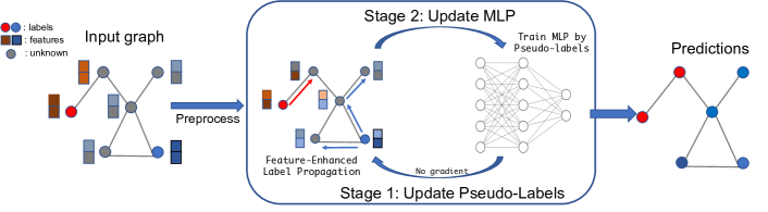
In this subsection, we detail the implementation of ALT-OPT. As shown in Figure 1, we first preprocess the node feature through a diffusion, then alternatively update pseudo label ${\mathbf{F}}$ and MLP while taking into account the weight of pseudo labels and the class balancing problem, and finally get the predictions. Next, we describe each step in detail.

Preprocessing. From Understanding 1 and 2, we use the pseudo labels generated by MLP to enhance the label propagation, so a good initialized MLP is needed. In real graphs, labeled data are usually scarce so it is challenging to get a good initialization of MLP with a small number of labels. Therefore, we first diffuse the original node features with its neighbors to get smoothing and enhanced features. The new features are obtained from ${\mathbf{X}}^{\prime}=\text{LP}({\mathbf{X}},\alpha)$. Then, we train MLP only using the labeled data for a few epochs to get an initialization, similar to pseudo-labeling methods (Iscen et al., 2019; Lee et al., 2013).

Update F. We initial ${\mathbf{F}}^{0}={\mathbf{Y}}$. Then we update ${\mathbf{F}}$ for labeled nodes and unlabeled nodes by Eq. (4) and Eq. (5), respectively. Since ${\mathbf{F}}$ acts as pseudo labels when training the MLP, we normalize ${\mathbf{F}}$ to be the distribution of classes by the softmax function with temperature after the update: ${\mathbf{F}}_{ij}=\frac{\exp\left({\mathbf{F}}_{ij}/\tau\right)}{\sum_{k=1}^{c}\exp\left({\mathbf{F}}_{ik}/\tau\right)}$, where $\tau$ is a hyperparameter to control the smoothness of pseudo labels.

Pseudo-labels Generation. Directly using all pseudo labels to train MLP is not appropriate due to the following reasons. First, not all pseudo labels have the same certainty. Second, pseudo-labels may not be balanced over classes, which will impede learning. To address the first issue, we assign a confidence weight to each pseudo-label (Rizve et al., 2021; Iscen et al., 2019). According to information theory, entropy can be used to quantify a distribution’s uncertainty, so we define the weight for unlabeled nodes as $w_{i}=1-\frac{H({\mathbf{F}}_{i})}{log(c)}$, where $w_{i}\in[0,1]$ and $H({\mathbf{F}}_{i})=-\sum_{j=1}^{c}{\mathbf{F}}_{ij}\log{\mathbf{F}}_{ij}$ is the entropy of the pseudo label ${\mathbf{F}}_{i}$. To deal with the class imbalance problem, we train the MLP using the same number of unlabeled nodes for each class with the highest weights.

Update MLP. We train MLP using both labeled nodes ${\mathcal{V}}_{L}$ and high confidence unlabeled nodes ${\mathcal{V}}_{U_{t}}$ with the loss:

$$\sum_{i\in{\mathcal{V}}_{L}}\ell({\text{MLP}}({\mathbf{X}}^{\prime}_{i};\Theta),{\mathbf{F}}_{i})+\sum_{j\in{\mathcal{V}}_{Ut}}w_{j}\cdot\ell({\text{MLP}}({\mathbf{X}}^{\prime}_{j};\Theta),{\mathbf{F}}_{j}),$$

where $\ell({\text{MLP}}({\mathbf{X}}^{\prime}_{i};\Theta),{\mathbf{F}}_{i})=\|{\text{MLP}}({\mathbf{X}}^{\prime}_{i};\Theta)-{\mathbf{F}}_{i}\|_{2}^{2}$ is a MSE loss and $\Theta$ is the parameters of MLP.

Prediction. The inference of the proposed method is based on the pseudo labels ${\mathbf{F}}$, and the predicted class for the unlabeled node $i$ can be obtained as $c_{i}=\arg\max_{j}{\mathbf{F}}_{ij}$.

It is important to note that the normalization of ${\mathbf{F}}$ and pseudo-label reweighting can be incorporated into the unified framework. Please refer to Appendix C for more details. The overall algorithm and implementation details  of ALT-OPT are shown in Appendix D.

3.6 Complexity Analysis

We provide time and memory complexity analyses for ALT-OPT and the following representative GNNs: GCN (Kipf & Welling, 2016), SGC (Wu et al., 2019a), and APPNP (Klicpera et al., 2018).

Suppose that $p$ is the number of propagation layers, $n$ is the number of nodes, $m$ is the number of edges, and $c$ is the number of classes. For simplicity, we assume that the hidden feature dimension is a fixed $d$ for all transformation layers, and we have $c\ll d$ in most cases; all feature transformations are updated $t$ epochs. The adjacent matrix ${\mathbf{A}}$ is a sparse matrix, and forward and backward propagation have the same cost. Following (Li et al., 2021), we only analyze the inherent differences across models by assuming that they have the same transformation layers (MLP), allowing us to disregard the time and memory footprint of MLP. The time and memory complexities are summarized in Table 1.

Time complexity. We first analyze the time complexity of feature aggregation. The feature aggregation can be implemented as a sparse-dense matrix multiplication with cost $O(md)$ if the feature has $d$ dimensions. Therefore, the time complexity of training a $p$-layer GCN for $t$ epochs is $O(2tpmd)$ with the gradient backpropagation. For SGC, we only need $p$ steps of feature propagation, so the time complexity is $O(pmd)$. For APPNP, the gradient also needs to backpropagate through $p$ layers, but the feature dimension is $c$, resulting in the time complexity of $O(2tpmc)$. Regarding ALT-OPT, as the model are optimized in an alternating way, there is no need to do both feature transformation and aggregation in each epoch. Rather, we can propagate the pseudo labels only for $k$ times during the whole training process. As a result, the time complexity of ALT-OPT is $O(kpmc)$. In practice, choosing $k$ from $\{2,3,4,5\}$ can achieve very promising performance, while $t$ needs to be 500 or 1,000 for other models to converge.

Table 1: Comparison of time and memory complexities.

Method	Time	Memory
GCN	$O(2tpmd)$	$O(nd+pnd)$
SGC	$O(pmd)$	$O(nd)$
APPNP	$O(2tpmc)$	$O(nd+pnc)$
ALT-OPT	$O(kpmc)$	$O(nd+nc)$

Memory complexity. All models require $O(nd)$ memory for storing node features. For the end-to-end training models, we need to store the intermediate state at each layer for gradient calculation. Specifically, for GCN, we need to store the hidden state for $p$ layers, so the memory complexity is $O((p+1)nd)$. SGC only needs to store the propagated feature $O(nd)$ as we omit the memory of network parameters. Similarly, APPNP has the memory complexity of $O(nd+pnc)$. As for ALT-OPT, it does not need to store the gradients at each propagation layer. Instead, ALT-OPT needs to hold the pseudo label ${\mathbf{F}}$. So the memory complexity of ALT-OPT is $O(nd+nc)$.

If we omit the difference in the dimension of the propagation features (d = c), the time and memory of GCN and APPNP are the same, as they are both Pesistent GNNs that require feature propagation in each epoch. Similarly, the One-time GNNs that only need to propagate once, such as SGC, SIGN, and C&S have the same time and memory complexity. ALT-OPT is a Lazy Propagation method since the features are propagated $k$ times during training with $k$ being a small number. Thus, ALT-OPT can be seen as a balance between these two groups of methods.

4 Experiment

In this section, we verify the effectiveness of the proposed ALT-OPT by comprehensive experiments. In particular, we try to answer the following questions:

• RQ1: How does ALT-OPT perform when compared to other baseline models?

• RQ2: Is ALT-OPT more time and memory efficient than state-of-the-art GNNs?

• RQ3: How do different components affect ALT-OPT?

4.1 Experimental settings

Datasets. For the transductive semi-supervised node classification task, we choose nine commonly used datasets including three citation datasets, i.e., Cora, Citeseer and Pubmed (Sen et al., 2008), two coauthors datasets, i.e., CS and Physics, two Amazon datasets, i.e., Computers and Photo (Shchur et al., 2018), and two OGB datasets, i.e., ogbn-arxiv and ogbn-products (Hu et al., 2020). For the inductive node classification task, we use Reddit and Flikcr datasets (Zeng et al., 2019). We also test the proposed method on two heterophily graphs, i.e., Chameleon and Squirrel (Pei et al., 2020). More details about these datasets are shown in Appendix E.

We use 10 random data splits for all the datasets except the OGB datasets. For the OGB datasets, we use the fixed data split. We run the experiments 3 times for each split and report the average performance and standard deviation. Besides, we also test multiple labeling rates, i.e., low label rates with 5, 10, 20, and 60 labeled nodes per class and high label rates with 30% and 60 % labeled nodes per class, to get a comprehensive comparison.

Baselines. We compare the proposed ALT-OPT with three groups of methods: (i) Persistent GNNs, i.e., GCN (Kipf & Welling, 2016), GAT (Veličković et al., 2017) and APPNP (Klicpera et al., 2018); (ii) One-time GNNs, i.e., SGC (Wu et al., 2019a), SIGN (Rossi et al., 2020), and C&S (Huang et al., 2020); and (iii) Non-GNN methods including MLP and Label Propagation (Zhou et al., 2003). We report the test accuracy selected by the the best validation accuracy. Parameter settings are summarized in Appendix F.

4.2 Performance Comparison on Benchmark Datasets

4.2.1 Transductive Node Classification.

The transductive node classification results are partially shown in Table 2. We leave results on more datasets and methods with more learning rate setting in Appendix G due to the space limitation. From these results, we can make the following observations:

• ALT-OPT consistently outperforms other models at low label rates on all datasets. For example, in Cora and CiteSeer with label rate 5, our method can gain $1.2\%$ and $5.6\%$ relative improvement compared to the best baselines. This is because the pseudo labels generated by our framework are helpful for training models when there are few labels available. When the label rate is high, our method is also comparable to the best results. In addition, ALT-OPT is alternately optimized, which suggests that end-to-end training could not be necessary for node semi-supervised classification.

• ALT-OPT performs the best on two OGB datasets. For example, in the large ogbn-products dataset, it obtains 7.86% and 2.63% relative improvement compared to APPNP and SIGN, respectively.

• Compared with the One-time GNNs, Persistent GNNs usually perform better when the labeling rate is low. In addition, the label propagation outperforms MLP in most cases, indicating the rationality of our proposed feature-enhanced label propagation.

• The standard deviation of all models is not small across different data splits, especially when the label rate is very low. It demonstrates that splits can significantly affect a model’s performance. A similar finding is also observed in the PyTorch-Geometric paper (Fey & Lenssen, 2019).

Table 2: Transductive node classification accuracy (%) on benchmark datasets.

Method		Persistent GNNs			One-time GNNs			Ours
Dataset	Label	GCN	GAT	APPNP	SGC	SIGN	C&S	ALT-OPT
Cora	5	70.68 $\pm$ 2.17	72.97 $\pm$ 2.23	75.86 $\pm$ 2.34	70.06 $\pm$ 1.95	69.81 $\pm$ 3.13	56.52 $\pm$ 5.53	76.78 $\pm$ 2.56
	10	76.50 $\pm$ 1.42	78.03 $\pm$ 1.17	80.29 $\pm$ 1.00	76.28 $\pm$ 1.22	76.25 $\pm$ 1.26	71.04 $\pm$ 3.30	80.66 $\pm$ 1.92
	20	79.41 $\pm$ 1.30	81.39 $\pm$ 1.41	82.34 $\pm$ 0.67	80.30 $\pm$ 1.72	79.71 $\pm$ 1.11	77.96 $\pm$ 2.13	82.66 $\pm$ 0.98
	60	84.30 $\pm$ 1.44	85.11 $\pm$ 1.10	85.49 $\pm$ 1.25	84.17 $\pm$ 1.39	84.16 $\pm$ 1.18	82.21 $\pm$ 1.45	85.60 $\pm$ 1.12
	30%	86.87 $\pm$ 1.35	87.24 $\pm$ 1.19	87.77 $\pm$ 1.13	86.97 $\pm$ 0.90	87.17 $\pm$ 1.28	87.60 $\pm$ 1.12	87.70 $\pm$ 1.19
CiteSeer	5	61.27 $\pm$ 3.85	62.60 $\pm$ 3.34	63.92 $\pm$ 3.39	60.21 $\pm$ 3.48	57.44 $\pm$ 3.71	50.39 $\pm$ 4.70	67.48 $\pm$ 2.90
	10	66.28 $\pm$ 2.14	66.81 $\pm$ 2.10	67.57 $\pm$ 2.05	65.23 $\pm$ 2.36	63.87 $\pm$ 3.09	58.96 $\pm$ 2.75	69.39 $\pm$ 2.59
	20	69.60 $\pm$ 1.67	69.66 $\pm$ 1.47	70.85 $\pm$ 1.45	68.82 $\pm$ 2.11	68.60 $\pm$ 1.94	65.85 $\pm$ 2.74	71.26 $\pm$ 1.69
	60	72.52 $\pm$ 1.74	73.10 $\pm$ 1.20	73.50 $\pm$ 1.54	71.43 $\pm$ 1.26	72.63 $\pm$ 1.39	71.21 $\pm$ 1.79	72.84 $\pm$ 1.65
	30%	75.20 $\pm$ 0.85	75.01 $\pm$ 0.99	75.71 $\pm$ 0.71	75.09 $\pm$ 1.01	74.44 $\pm$ 0.83	74.65 $\pm$ 0.95	75.09 $\pm$ 0.79
Pubmed	5	69.76 $\pm$ 6.46	70.42 $\pm$ 5.36	72.68 $\pm$ 5.68	68.55 $\pm$ 6.88	66.52 $\pm$ 6.15	65.3 $\pm$ 6.02	73.51 $\pm$ 4.80
	10	72.79 $\pm$ 3.58	73.35 $\pm$ 3.83	75.53 $\pm$ 3.85	72.80 $\pm$ 3.55	71.32 $\pm$ 3.70	72.51 $\pm$ 3.75	75.55 $\pm$ 5.09
	20	77.43 $\pm$ 1.93	77.43 $\pm$ 2.66	78.93 $\pm$ 2.11	76.48 $\pm$ 2.84	76.39 $\pm$ 2.65	75.34 $\pm$ 2.49	79.16 $\pm$ 2.26
	60	82.00 $\pm$ 1.62	81.40 $\pm$ 1.40	82.55 $\pm$ 1.47	80.34 $\pm$ 1.61	81.75 $\pm$ 1.55	80.63 $\pm$ 1.49	82.53 $\pm$ 1.76
	30%	88.07 $\pm$ 0.29	86.51 $\pm$ 0.41	87.56 $\pm$ 0.39	86.23 $\pm$ 0.43	89.09 $\pm$ 0.33	88.44 $\pm$ 0.40	88.24 $\pm$ 0.36
CS	20	91.73 $\pm$ 0.49	90.96 $\pm$ 0.46	92.38 $\pm$ 0.38	90.32 $\pm$ 0.99	92.02 $\pm$ 0.41	92.41 $\pm$ 0.44	92.77 $\pm$ 0.50
Physics	20	93.29 $\pm$ 0.80	92.81 $\pm$ 1.03	93.49 $\pm$ 0.67	93.23 $\pm$ 0.59	93.03 $\pm$ 1.15	93.23 $\pm$ 0.55	94.63 $\pm$ 0.31
Computers	20	79.17 $\pm$ 1.92	78.38 $\pm$ 2.27	79.07 $\pm$ 2.34	73.00 $\pm$ 2.0	73.04 $\pm$1.15	73.25$\pm$ 2.09	79.12 $\pm$ 2.50
Photo	20	89.94 $\pm$ 1.22	89.24 $\pm$ 1.42	90.87 $\pm$ 1.14	83.50 $\pm$ 2.9	86.11 $\pm$ 0.66	84.87 $\pm$ 1.04	91.23 $\pm$ 1.26
ogbn-arxiv	54%	71.91 $\pm$ 0.15	71.92 $\pm$ 0.17	71.61 $\pm$ 0.30	68.74 $\pm$ 0.12	71.95 $\pm$ 0.11	71.03 $\pm$ 0.15	72.76 $\pm$ 0.17
ogbn-products	8%	75.70 $\pm$ 0.19	OOM	76.62 $\pm$ 0.13	74.29 $\pm$ 0.12	80.52$\pm$0.16	77.11 $\pm$ 0.06	82.64$\pm$ 0.21

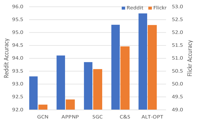
4.2.2 Inductive Node Classification.

For inductive node classification, only training nodes can be observed in the graph during training, and all nodes can be used during the inference (Zeng et al., 2019). For ALT-OPT, we first train an MLP with the original features and then do inference for the unlabeled node using the feature-enhanced label propagation in Eq (4) and Eq (5).

As shown in Figure 2 and Appendix H, our ALT-OPT outperforms other baselines on the inductive node classification task. The only difference between ALT-OPT and MLP is the feature-enhanced label propagation, but our method can achieve 52.3% and 38.1 % relative improvement compared to MLP. The performance improvement can demonstrate the superiority of our feature-enhanced label propagation.

Figure 2: Inductive node classification accuracy (%).

4.2.3 Performance on Heterophily Graphs.

ALT-OPT is a specific instance of the proposed single-level optimization framework. It utilizes graph Laplacian regularization, expressed as ${\mathrm{tr}}({\mathbf{F}}^{\top}{\tilde{{\mathbf{L}}}}{\mathbf{F}})$, to constrain node features with the graph structure. The Laplacian regularization is a low-pass filter, potentially limiting its performance with heterophily graphs, where high-frequency signals are helpful.

Nonetheless, the proposed Eq. (2) serves as a general framework, permitting the incorporation of different filters to seize the high-frequency signals prevalent in heterophily graphs. To illustrate this, we introduce a novel regularization term, denoted as ${\mathcal{D}}_{A}={\mathrm{tr}}({\mathbf{F}}^{\top}{\tilde{{\mathbf{L}}}}^{2}{\mathbf{F}})$, which is capable of capturing both low-pass and high-pass graph signals. Consequently, this results in a new method, which we term ALT-OPT-H for brevity. The specifics of this method are as follows:

$${\mathcal{L}}=\lambda_{1}\underbrace{\|{\text{MLP}}({\mathbf{X}})-{\mathbf{F}}\|_{F}^{2}}_{{\mathcal{D}}_{X}}+\underbrace{{\mathrm{tr}}({\mathbf{F}}^{\top}{\tilde{{\mathbf{L}}}}^{2}{\mathbf{F}})}_{{\mathcal{D}}_{A}}+\lambda_{2}\underbrace{\|{\mathbf{F}}_{L}-{\mathbf{Y}}_{L}\|_{F}^{2}}_{{\mathcal{D}}_{Y}},$$

which can be solved using the same alternating optimization method as in Equation (3). We carry out experiments on two of the most widely utilized heterophily datasets, namely Chameleon and Squirrel. We maintain the same settings as in the study by Lim et al. (2021), and compare several renowned heterophily GNNs, such as Geom-GCN (Pei et al., 2020), H₂GCN (Zhu et al., 2020a), MixHop (Abu-El-Haija et al., 2019), GCNII (Chen et al., 2020), GPR-GNN (Chien et al., 2020), and LINKX (Lim et al., 2021). The results in Table 3 show that our ALT-OPT-H method displays competitive performance on heterophily datasets, necessitating only a slight adjustment to the graph filter. This attests to the flexibility of the proposed framework (Eq. (2)), which can perform well on both homophily and heterophily graphs.

Table 3: Performance on the heterophily graphs.

Dataset	Chameleon	Squirrel
Geom-GCN	60.90	38.14
H2GCN	59.39 ± 1.98	37.90 ± 2.02
MixHop	60.50 ± 2.53	43.80 ± 1.48
GCNII	62.48	56.63 ± 1.17
GPR-GNN	62.85 ± 2.90	54.35 ± 0.87
LINKX	68.42 ± 1.38	61.81 ± 1.80
ALT-OPT-H	70.62 ± 1.93	61.56 ± 1.81

4.3 Efficiency Comparison

In this subsection, we compare the efficiency of our ALT-OPT with other baselines, based on two large datasets, i.e., ogbn-arxiv and ogbn-products. To make a fair comparison, we choose the same feature transformation layers for each method. Besides, we update model parameters with the same iterations in each method, i.e., 500 epochs for ogbn-arxiv and 1,000 epochs for ogbn-products. All the experiments are conducted on the same machine with a NVIDIA RTX A6000 GPU (48 GB memory). For ALT-OPT, we can update ${\mathbf{F}}$ with different frequencies in training, i.e., 1, 2, 3, 4, 5, and “Full”. “Full” means we update both ${\mathbf{F}}$ and MLP in each epoch. For ALT-OPT-$k$, we only update the ${\mathbf{F}}$ for $k$ times during the training procedure. The overall results are shown in Table 4.

Training Time. For the Persistent GNNs including GCN, APPNP and ALT-OPT-Full, the training time is longer than other methods that do not need to propagate every epoch. Both APPNP and ALT-OPT-Full need to propagate ten layers every epoch and GCN needs to propagate three layers. However, the training time of ALT-OPT-Full is nearly half of APPNP and still less than GCN, which matches our time complexity analysis in Section 3.6, as there is no gradient backpropagate through propagation layers. Compared with the One-time GNNs like SGC, ALT-OPT with only a few update steps, such as ALT-OPT-5, can achieve better accuracy with a minor increase in training time. For example, the whole training time of ALT-OPT-5 is only 0.92s and 7s longer than SGC, but it has 8.63% and 11.24 % relative performance improvements in ogbn-arxiv and ogbn-products datasets, respectively. Meanwhile, we observe that ALT-OPT-5 has very similar performance with ALT-OPT-Full, which suggests that there is no need to do propagation and train the model simultaneously for each epoch. This also suggests that end-to-end training with propagation might not be necessary.

Memory Cost. Compared with the Persistent GNNs, ALT-OPT requires less memory with no requirement to store the hidden states in the propagation layers. Thus, ALT-OPT can keep a constant memory even with more propagation layers. Compared with MLP and SGC, ALT-OPT shows comparable memory. Slightly memory increasing is from the pseudo label matrix as analyzed in Section 3.6. ALT-OPT can be even more efficient with sampling strategies.

Table 4: Efficiency comparison of different methods.

Dataset	ogbn-arxiv			ogbn-products
Method	ACC(%)	Time (s)	Memory (GB)	ACC (%)	Time (s)	Memory (GB)
MLP	55.68	12.01	2.68	61.17	214	21.18
SGC	66.92	12.06	2.71	74.29	215	21.85
SIGN	71.95	24.89	4.67	80.52	492	43.17
GCN	71.91	24.71	3.33	75.70	1,284	38.36
APPNP	71.61	33.70	3.20	76.62	1,913	29.15
ALT-OPT-Full	72.76	22.28	2.81	81.83	901	24.49
ALT-OPT-1	70.09	12.86	2.81	80.03	218	24.49
ALT-OPT-2	72.32	12.89	2.81	80.34	219	24.49
ALT-OPT-3	72.60	12.92	2.81	81.00	220	24.49
ALT-OPT-4	72.71	12.95	2.81	81.89	221	24.49
ALT-OPT-5	72.70	12.98	2.81	82.64	222	24.49

In Appendix I, we also provide additional experiments to show the efficiency of our ALT-OPT, i.e. ALT-OPT can converge faster, need fewer propagation layer, and the memory cost does not increase with more propagation layers.

4.4 Ablation Study

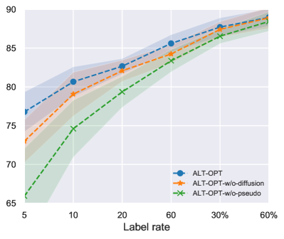
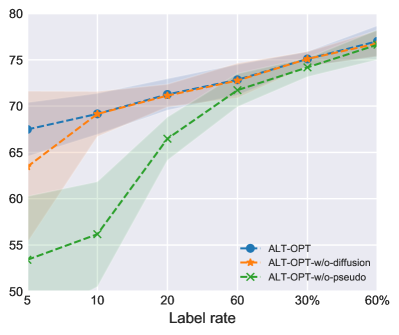
Feature Diffusion. It is expected that feature diffusion can improve the accuracy of the MLP in the pretraining procedure and thus improve the initialization quality of pseudo labels ${\mathbf{F}}$. To validate this, we remove the feature diffusion and also use the pseudo labels to train our method, which is called ALT-OPT-w/o-diffusion. Experiments are conducted on Cora and CiteSeer datasets. From Figure 3, we can see that at low label rates, ALT-OPT is better than ALT-OPT-w/o-diffusion which means that feature diffusion can boost the model’s performance at low labeling rate. As the labeling rate increases, the performance gap becomes small. This shows that feature diffusion is not the key component in our method when the label rate is not very low.

Pseudo Labels. One of the most important advantages of ALT-OPT is that we leverage pseudo labels to better train MLP. To study the contribution of pseudo labels in ALT-OPT, we test the model variant ALT-OPT-w/o-pseudo which only uses labeled data on Cora and CiteSeer datasets. Compared with ALT-OPT, Figure 3 shows that pseudo labels have a large impact on model performance on both datasets, especially when the label rate is low.

(a) Cora

(b) CiteSeer

Figure 3: Performance of ALT-OPT variants.

Moreover, we choose the top $K$ confidence pseudo labels per class after the first update of ${\mathbf{F}}$ to verify their accuracy. We adopt the same way to evaluate Label Propagation on Cora dataset with the label rate 20. As shown in Figure 4, after the first update of ${\mathbf{F}}$, the accuracy of the top 180 nodes from each class can be $90\%$. So it is reasonable to use these pseudo labels to train MLP. Besides, the accuracy of our method at each K is much better than Label propagation, which suggests the effectiveness of the feature-enhanced label propagation update for ${\mathbf{F}}$.

Hyperparameters Sensitivity. We test the parameter sensitivity of $\lambda_{1}$ and $\lambda_{2}$ in Eq (3) on Physics and Photo datasets by fixing one with the best parameters and tuning the other. From Figure 5, ALT-OPT is not very sensitive to these two hyperparameters at the chosen regions.

Figure 4: Top K Accuracy.

Figure 5: Parameter Sensitivity.

5 Related Works

Graph Neural Networks (GNNs) is an effective architecture to represent the graph-structure data, and there are mainly two operators, i.e. feature transformation and propagation. Based on the order of these two operators, most GNNs can be classified into: Coupled and Decoupled GNNs. Coupled GNNs, such as GCN (Kipf & Welling, 2016), GraphSAGE (Hamilton et al., 2017), and GAT (Velickovic et al., 2017), couple feature transformation and propagation in each layer. More recently, decoupled GNNs, such as APPNP (Klicpera et al., 2018), that decouple the transformation and propagation, are proposed to alleviate the over-smoothness problem (Li et al., 2018; Oono & Suzuki, 2019). Similar architectures are also utilized in (Liu et al., 2021, 2020; Zhou et al., 2021).

In this paper, we categorize GNNs into Persistent GNNs and One-time GNNs. One-time GNNs, such as SGC (Wu et al., 2019a), SIGN (Rossi et al., 2020) and C&S (Huang et al., 2020), are more efficient than the Persistent GNNs because they only propagate once. PTA (Dong et al., 2021) first propagate labels once and then train an MLP, which can be viewed as a One-time GNNs. PPRGo (Bojchevski et al., 2020) precomputes the PageRank matrix to avoid multiple steps of propagation, but it still need to do propagation in each epoch, which is also a Persistent GNN. However, our ALT-OPT does not belong to Coupled/Decoupled or Persistent/One-time GNNs. We propose a new learning paradigm for graph node classification task, which is both efficient and effective.

There are also many sampling methods (Hamilton et al., 2017; Chen et al., 2018; Zeng et al., 2019; Zou et al., 2019) that adopt mini-batch training strategies to reduce computation and memory cost by sampling some nodes and edges. Distributed methods (Chiang et al., 2019; Shao et al., 2022) distribute the large graph across multiple servers for parallel training. These works are orthogonal to the contributions in this work and they can be also applied to this work.

ALT-OPT can be understood as a pseudo-labeling method as discussed in Section 3.4. Recent work (Iscen et al., 2019) utilizes the label propagation to generate the pseudo labels, which shares some similarity with the proposed ALT-OPT. However, they use the features to generate graph at each iteration, and only the ground truth labels are leveraged for label propagation. For ALT-OPT, the propagation is a feature enhanced label propagation. We propagate both ground truth labels and features through the given graph. Besides, ALT-OPT is derived from our proposed framework by an alternating optimization algorithm, which has a different starting point than that of Iscen et al. (2019).

6 Conclusion

In this work, we demonstrate that most existing end-to-end GNNs for node classification are solving a bi-level optimization problem. We introduce a new optimization framework for node classification, which can efficiently be optimized with the alternating optimization algorithm. Experimental results validate that ALT-OPT is both computationally and memory efficient with promising performance on node classification, especially when the labeling rate is low.

Appendix A ALT-OPT with Cross Entropy Loss

In section 3.2, we instance ALT-OPT with a Mean Square Error Loss. In this section, we show it can be replaced by a Cross Entropy Loss. By replacing the first part of Eq (3) to be a cross entropy between MLP and ${\mathbf{F}}$, the formulation becomes:

$$\mathcal{L}=\lambda_{1}CE\Big{(}{\text{MLP}}({\mathbf{X}}),{\mathbf{F}}\Big{)}+{\mathrm{tr}}({\mathbf{F}}^{\top}{\tilde{{\mathbf{L}}}}{\mathbf{F}})+\lambda_{2}\|{\mathbf{F}}_{L}-{\mathbf{Y}}_{L}\|_{F}^{2}$$ (7)

where $CE(\cdot,\cdot)$ is the cross entropy function. Adopting the same gradient decent method, the update rule for ${\mathbf{F}}$ becomes:

$${\mathbf{F}}^{k+1}_{L} ={\mathbf{F}}^{k}_{L}-\eta_{L}\left(-\lambda_{1}\log{\text{MLP}}({\mathbf{X}}_{L})+2({\tilde{{\mathbf{L}}}}{\mathbf{F}}^{k})_{L}+2\lambda_{2}({\mathbf{F}}^{k}_{L}-{\mathbf{Y}}_{L})\right)$$

$$=\left(1-2\eta_{L}\left(1+\lambda_{2}\right)\right){\mathbf{F}}^{k}_{L}+\eta_{L}\lambda_{1}\log{\text{MLP}}(X)_{L}+2\eta_{L}{\tilde{{\mathbf{A}}}}{\mathbf{F}}^{k}_{L}+2\eta_{L}\lambda_{2}{\mathbf{Y}}_{L},$$ (8)

$${\mathbf{F}}^{k+1}_{U} ={\mathbf{F}}^{k}_{U}-\eta_{U}\left(-\lambda_{1}\log{\text{MLP}}({\mathbf{X}}_{U})+2({\tilde{{\mathbf{L}}}}{\mathbf{F}}^{k})_{U}\right)$$

$$=\left(1-2\eta_{U}\right){\mathbf{F}}^{k}_{U}+\eta_{U}\lambda_{1}\log{\text{MLP}}({\mathbf{X}}_{U})+2\eta_{U}({\tilde{{\mathbf{A}}}}{\mathbf{F}}^{k})_{U}$$ (9)

where the MLP is the output after the Softmax function and the step size can be set as $\eta_{L}=\eta_{U}=\frac{1}{2(1+\lambda_{2})}$. Therefore, the update rule of ${\mathbf{F}}$ is:

$${\mathbf{F}}^{k+1}_{L} =\frac{\lambda_{1}}{2\left(1+\lambda_{2}\right)}\log{\text{MLP}}({\mathbf{X}}_{L})+\frac{1}{1+\lambda_{2}}({\tilde{{\mathbf{A}}}}{\mathbf{F}}^{k})_{L}+\frac{\lambda_{2}}{1+\lambda_{2}}{\mathbf{Y}}_{L},$$ (10)

$${\mathbf{F}}^{k+1}_{U} =\frac{\lambda_{1}}{2(1+\lambda 2)}\log{\text{MLP}}({\mathbf{X}}_{U})+\frac{1}{1+\lambda_{2}}({\tilde{{\mathbf{A}}}}{\mathbf{F}}^{k})_{U}+\frac{\lambda_{2}}{1+\lambda_{2}}{\mathbf{F}}^{k}_{U}$$ (11)

Then we can consider the hidden variable ${\mathbf{F}}$ as pseudo label and update the parameters of MLP based on the cross entropy loss $CE({\text{MLP}},{\mathbf{F}})$. In practice, there are some situations that the cross entropy have a better performance than the original mean square error loss. Using two different losses would give similar results in most cases, and we report the best one.

Appendix B Understandings of ALT-OPT

B.1 Comparison between updating F and Label Propagation

Label Propagation (LP) (Zhou et al., 2003) is a well-known graph semi-supervised learning method based on the label smoothing assumption that connected nodes are likely to have the same label. The label propagation can be written as solving an the following optimization problem:

$$\begin{aligned} \mathcal{Q}({\mathbf{P}})&=\frac{1}{2}\sum_{i,j=1}^{n}A_{ij}\left\|\frac{1}{\sqrt{D_{ii}}}{\mathbf{P}}_{i}-\frac{1}{\sqrt{D_{jj}}}{\mathbf{P}}_{j}\right\|^{2}+\mu\sum_{i=1}^{n}\left\|{\mathbf{P}}_{i}-{\mathbf{Y}}_{i}\right\|^{2}\\ &=tr({\mathbf{P}}^{\top}{\tilde{{\mathbf{L}}}}{\mathbf{P}})+\mu\|{\mathbf{P}}-{\mathbf{Y}}\|_{F}^{2}\end{aligned}$$ (12)

We can use an iteration algorithm to solve Eq. 12. The $k$-th iteration process of LP is as follows:

$${\mathbf{P}}(k)=(1-\alpha){\tilde{{\mathbf{A}}}}{\mathbf{P}}(k-1)+\alpha{\mathbf{Y}},$$ (13)

where ${\tilde{{\mathbf{A}}}}$ is the normalized graph Laplacian matrix, ${\mathbf{Y}}$ is the label matrix, ${\mathbf{P}}(0)={\mathbf{Y}}$, and $\alpha\in(0,1)$ is a hyperparamter.

If we iterate Eq. 13 for one time, the ${\mathbf{P}}(k)$ becomes:

$$\begin{aligned} {\mathbf{P}}(k)&=(1-\alpha){\tilde{{\mathbf{A}}}}\left((1-\alpha){\tilde{{\mathbf{A}}}}{\mathbf{P}}(k-2)+\alpha{\mathbf{Y}}\right)+\alpha{\mathbf{Y}},\\ &=(1-\alpha)^{2}{\tilde{{\mathbf{A}}}}^{2}{\mathbf{P}}(k-2)+\alpha(1-\alpha){\tilde{{\mathbf{A}}}}{\mathbf{Y}}+\alpha{\mathbf{Y}}\end{aligned}$$ (14)

By iterating $K$ times, we can get:

$$\begin{aligned} {\mathbf{P}}(K)&=(1-\alpha)^{K}{{\tilde{{\mathbf{A}}}}}^{K}{\mathbf{Y}}+\alpha\sum_{k=0}^{K-1}(1-\alpha)^{k}{\tilde{{\mathbf{A}}}}^{k}{\mathbf{Y}}\\ &=\left((1-\alpha)^{K}{{\tilde{{\mathbf{A}}}}}^{K}+\alpha\sum_{k=0}^{K-1}(1-\alpha)^{k}{\tilde{{\mathbf{A}}}}^{k}\right){\mathbf{Y}}\\ &=\bar{{\mathbf{A}}}{\mathbf{Y}}\end{aligned}$$ (15)

Let $\bar{{\mathbf{A}}}=(1-\alpha)^{K}{{\tilde{{\mathbf{A}}}}}^{K}+\alpha\sum_{k=0}^{K-1}(1-\alpha)^{k}{\tilde{{\mathbf{A}}}}^{k}$, then the $K$ step LP can be represented as $LP({\mathbf{Y}},\alpha)=\bar{{\mathbf{A}}}{\mathbf{Y}}$. For our ALT-OPT, our optimization problem is:

$$\mathcal{L}=\lambda_{1}\|{\text{MLP}}({\mathbf{X}})-{\mathbf{F}}\|_{F}^{2}+{\mathrm{tr}}({\mathbf{F}}^{\top}{\tilde{{\mathbf{L}}}}{\mathbf{F}})+\lambda_{2}\|{\mathbf{F}}-{\mathbf{Y}}\|_{F}^{2},$$

which can also be written as

$${\mathbf{F}}(k) =\frac{1}{\lambda_{1}+\lambda_{2}+1}{\tilde{{\mathbf{A}}}}{\mathbf{F}}(k-1)+\frac{\lambda_{1}}{\lambda_{1}+\lambda_{2}+1}{\text{MLP}}({\mathbf{X}})+\frac{\lambda_{2}}{\lambda_{1}+\lambda_{2}+1}{\mathbf{Y}}.$$ (16)

By iterating Eq. 16, it becomes:

$$\begin{aligned} {\mathbf{F}}(k)=\left((\frac{1}{\lambda_{1}+\lambda_{2}+1})^{K}{{\tilde{{\mathbf{A}}}}}^{K}+\frac{\lambda_{1}+\lambda_{2}}{\lambda_{1}+\lambda_{2}+1}\sum_{k=0}^{K-1}(\frac{1}{\lambda_{1}+\lambda_{2}+1})^{k}{\tilde{{\mathbf{A}}}}^{k}\right)\left(\frac{\lambda_{1}}{\lambda_{1}+\lambda_{2}+1}{\text{MLP}}({\mathbf{X}})+\frac{\lambda_{2}}{\lambda_{1}+\lambda_{2}+1}{\mathbf{Y}}\right)\end{aligned}$$ (17)

Let $\alpha=\frac{\lambda_{1}+\lambda_{2}}{\lambda_{1}+\lambda_{2}+1},\beta=\frac{\lambda_{2}}{\lambda_{1}+\lambda_{2}+1}$, Eq. 17 can be written as:

$${\mathbf{F}}(K)=\bar{{\mathbf{A}}}\left((\alpha-\beta){\text{MLP}}({\mathbf{X}})+\beta{\mathbf{Y}}\right).$$ (18)

Compared Eq. 12 with Eq. 18, ALT-OPT not only propagates the ground truth labels, but “feature” labels ${\text{MLP}}({\mathbf{X}})$ generated by features. Thus, updating ${\mathbf{F}}$ takes advantage of all node features, graph structure and labels, while LP only leverages graph structure and labels. Thus, updating ${\mathbf{F}}$ of ALT-OPT can be seen as a feature-enhanced label propagation.

B.2 Comparison between updating $\Theta$ and pseudo-labeling methods

Pseudo-labeling (Lee et al., 2013; Arazo et al., 2020) is a popular method in semi-supervised learning that uses a small set of labeled data along with a large amount of unlabeled data to improve model performance. It usually generates pseudo labels for the unlabeled data and trains the deep models using both the true labels and pseudo labels with different weights. From this perspective, ALT-OPT uses the pseudo labels ${\mathbf{F}}$ to train MLP.

Let $\boldsymbol{f}_{\theta}(\boldsymbol{X})={\text{MLP}}(X)$, the loss function for training ALT-OPT can be written as the following based on Eq. 18:

$$L_{\textsc{ALT-OPT}} =\ell\left(\boldsymbol{f}_{\theta}(\boldsymbol{X}),\overline{\boldsymbol{A}}((\alpha-\beta)\boldsymbol{f}_{\theta}(\boldsymbol{X})^{\prime}+\beta\boldsymbol{Y})\right),$$ (19)

where $\boldsymbol{f}_{\theta}(\boldsymbol{X})^{\prime}$ is the output from previous layer, and there is no gradient information.

If we choose Cross Entropy loss, then Eq. 19 becomes:

$$\begin{aligned} L_{\textsc{ALT-OPT}}&=-\sum_{i,j\in{\mathcal{V}}}\sum_{k\in{\mathcal{C}}}\bar{a}_{ij}((\alpha-\beta)f_{\theta}({\mathbf{X}})_{j,k}^{\prime}+\beta{\mathbf{Y}}_{jk})logf_{\theta}({\mathbf{X}})_{i,k}\\ &=-(\alpha-\beta)\sum_{i,j\in{\mathcal{V}}}\sum_{k\in{\mathcal{C}}}\bar{a}_{ij}f_{\theta}({\mathbf{X}})_{j,k}^{\prime}logf_{\theta}({\mathbf{X}})_{i,k}-\beta\sum_{i,j\in{\mathcal{V}}}\sum_{k\in{\mathcal{C}}}{\mathbf{Y}}_{jk})logf_{\theta}({\mathbf{X}})_{i,k}\\ &=-(\alpha-\beta)\sum_{i,j\in{\mathcal{V}}}\sum_{k\in{\mathcal{C}}}\bar{a}_{ij}f_{\theta}({\mathbf{X}})_{j,k}^{\prime}logf_{\theta}({\mathbf{X}})_{i,k}-\beta\sum_{i,j\in{\mathcal{V}}}\sum_{k\in{\mathcal{C}}}\bar{a}_{ij}{\mathbf{Y}}_{jk}logf_{\theta}({\mathbf{X}})_{i,k}\\ &=-(\alpha-\beta)\sum_{i,j\in{\mathcal{V}}}\sum_{k\in{\mathcal{C}}}\bar{a}_{ij}f_{\theta}({\mathbf{X}})_{j,k}^{\prime}logf_{\theta}({\mathbf{X}})_{i,k}-\beta\sum_{i\in{\mathcal{V}},j\in{\mathcal{V}}_{L}}{\mathbf{Y}}_{jh(j)}logf_{\theta}({\mathbf{X}})_{i,h(j)}\\ &=(\alpha-\beta)\sum_{i,j\in{\mathcal{V}}}\bar{a}_{ij}CE(f_{i},f_{j}^{\prime})+\beta\sum_{i\in{\mathcal{V}},j\in{\mathcal{V}}_{L}}\bar{a}_{ij}CE(f_{i},y_{j}),\end{aligned}$$ (20)

where $h(j)$ is the label of labeled node $j$, thus ${\mathbf{Y}}_{j,k}=1$ if $k=h(j)$ else ${\mathbf{Y}}_{j,k}=0$. From Eq. 20, we can find that ALT-OPT use both truth label $y_{i}$ and pseudo label $f_{j}^{\prime}$ to train the MLP.

Appendix C Incorporating Normalization and Pseudo-label Reweighting into a Unified Framework

In our ALT-OPT implementation, we utilize normalization to map the feature into a label space and a pseudo-label reweighting operator to select high-confidence nodes for training MLP. These operations cannot be directly derived from Eq. 3. However, by slightly modifying our approach, we can integrate these two operators into a unified framework. Specifically, we use the softmax function to map $\mathbf{F}$ into the label space and a diagonal weight matrix to reweight pseudo-labels. Let $softmax(\mathbf{F})=S(\mathbf{F})$. We can then modify the optimization target as follows:

$$L=\lambda_{1}\mathbf{W}CE(MLP(\mathbf{X}),S(\mathbf{F}))+\operatorname{tr}\left(\mathbf{F}^{\top}\tilde{\mathbf{L}}\mathbf{F}\right)+\lambda_{2}CE(Y,S(\mathbf{F})),$$ (21)

where CE is the Cross-Entropy function, the weight matrix $\mathbf{W}$ is a diagonal matrix, $w_{q}=w_{q}^{\prime}\mathbbm{1}\left(w^{\prime}_{q}>\tau\right)$, $w^{\prime}_{q}=Entropy(softmax(\mathbf{F}_{q})))$, $\mathbbm{1}$ is the indicator function, and $\tau$ is a threshold. The reason we adopt the Cross-Entropy function is that it has a neat derivative with the Softmax operator, i.e. $\frac{\partial{CE(\mathbf{Y},S(\mathbf{F}))}}{\partial{\mathbf{F}}}=S(\mathbf{F})-\mathbf{Y}$.

Therefore, the gradient of $\mathcal{L}$ with respect to $\mathbf{F}$ is:

$$\frac{\partial{L}}{\partial{F}}=\lambda_{1}\mathbf{W}(S(\mathbf{F})-MLP(\mathbf{X}))+2\mathbf{L}\mathbf{F}+\lambda_{2}(S(\mathbf{F})-Y).$$ (22)

This gradient closely resembles the original one with the MSE loss, making the optimization target quite tidy and similar to the original one. This problem can be resolved using the same alternating optimization method as before. We term the new method as ALT-OPT-N. To evaluate our proposed method, we chose three representative datasets, namely, PubMed, Coauthor CS, and ogbn-arxiv. The results are as follows:

Table 5: Different implementations of ALT-OPT

Dataset	PubMed	CS	ogbn-arxiv
ALT-OPT	79.16 ± 2.26	92.77 ± 0.50	72.60
ALT-OPT-N	78.66 ± 2.00	92.69 ± 0.28	72.58

The results show that ALT-OPT-N achieves performance similar to ALT-OPT, with all operators being derivable from ALT-OPT-N. This underlines the efficacy of our proposed unified framework for incorporating normalization and pseudo-label reweighting.

Appendix D Algorithm of ALT-OPT

In this section, we provide the algorithm 1 of ALT-OPT.

We first initialize the pseudo label ${\mathbf{F}}$ as label matrix ${\mathbf{Y}}$, and then preprocess data by feature diffusion. Afterward, we pre-train the MLP on the labeled data for a few epochs. Then, we update ${\mathbf{F}}$ and MLP alternatively and iteratively.

Algorithm 1 Algorithm of ALT-OPT

  Input: Adjacent matrix ${\mathbf{A}}$, Features ${\mathbf{X}}$, Labels ${\mathbf{Y}}$, Hyperparamters $\lambda_{1},\lambda_{2},\alpha$, pseudo label number $m$, pretraining steps $s$, MLP update times $t$

  Output: Pseudo Label ${\mathbf{F}}$, MLP parameter $\Theta$

  Initialize ${\mathbf{F}}={\mathbf{Y}}$

  ${\mathbf{X}}^{\prime}=LP({\mathbf{X}},\alpha)$

  for $i=1$ to $s$ do

     Pretrain MLP by $\mathcal{L}=\sum_{i\in L}\ell({\text{MLP}}(x^{\prime}_{i};\Theta),{\mathbf{Y}}_{i})$

  end for

  repeat

     Update ${\mathbf{F}}$ based on Eq. (4) and Eq. (5)

     Normalize ${\mathbf{F}}$ based on ${\mathbf{F}}_{ij}=\frac{\exp\left({\mathbf{F}}_{ij}/\tau\right)}{\sum_{k=1}^{C}\exp\left({\mathbf{F}}_{ik}/\tau\right)}$

     Select $m$ top unlabeled nodes $U_{t}$ per class by $w_{i}=1-\frac{H({\mathbf{F}}_{i})}{log(C)}$

     for $i=1$ to $t$ do

        Update $\Theta$ by minimizing $\mathcal{L}_{MLP}(X^{\prime},F;\Theta)=\sum_{i\in L\cup U_{t}}w_{i}\ell({\text{MLP}}(x^{\prime}_{i};\Theta),{\mathbf{F}}_{i})$

     end for

  until Model Converge

Appendix E Datasets Statistics

In the experiments, the data statistics used in Section 4 are summarized in Table 6. For Cora, CiteSeer and PubMed dataset, we adopt different label rates, i.e., 5, 10, 20, 60, 30% and 60% labeled nodes per class, to get a more comprehensive comparison. For label rates 5, 10, 20, and 60, we use 500 nodes for validation and 1000 nodes for test. For label rates 30% and 60%, we use half of the rest nodes for validation and the remaining half for test. For each labeling rate, we adopt 10 random splits for each dataset. For other datasets, we follow the original data split.

Table 6: Dataset Statistics.

Dataset	Nodes	Edges	Features	Classes
Cora	2,708	5,278	1,433	7
CiteSeer	3,327	4,552	3,703	6
PubMed	19,717	44,324	500	3
Coauthor CS	18,333	81,894	6,805	15
Coauthor Physics	34,493	247,962	8,415	5
Amazon Computer	13,381	245,778	767	10
Amazon Photo	7,487	119,043	745	8
Flickr	89,250	899,756	500	7
Reddit	232,965	11,606,919	602	41
Ogbn-Arxiv	169,343	1,166,243	128	40
Ogbn-Products	2,449,029	61,859,140	100	47

Appendix F Parameters Setting

In this section, we describe in detail the search space for parameters of different experiments.

F.1 Transductive Setting

For all deep models, we use 3 transformation layers with 256 hidden units for OGB datasets, and 2 transformation layers with 64 hidden units for other datasets. For all methods, the following hyperparameters are tuned based on the loss and validation accuracy from the following search space:

• Learning Rate: {0.01, 0.05}

• Dropout Rate: {0, 0.5, 0.8}

• Weight Decay: { 5e-4, 5e-5, 0}

• Hyperparamters between 0 and 1: step size 0.1

The propagation layers for APPNP and C&S is tuned from {5, 10} and {10, 20, 50}, respectively.

For ALT-OPT, the $\lambda_{1}$ and $\lambda_{2}$ are tuned from {0.1, 0.3, 0.5, 0.7, 1} and {1, 3, 5, 7, 10}, respectively; 10 propagation layers; pretraining steps $s=100$; $\tau=0.1$; pseudo label numbers per class $m$ are choose from {100, 200, 500, 5000} based on the size of graphs; The training epochs e is set to 1,000 for ogbn-products dataset and 500 for all other datasets same as other models. Then, a propagation times k is chosen (for example 5). Afterwards, we evenly split the training epochs $e$ to $k$ parts. For the first $e/k$ epochs, we train the MLP, and then do propagation once. For the next $e/k$ epochs we train the $MLP$ and then propagate once, and so on.

The Adam optimizer(Kingma & Ba, 2014) is used in all experiments.

F.2 Inductive Setting

For the inductive node classification task, we follow the data process as previous work (Zeng et al., 2019). Specifically, we first filter the training graph that only contains labeled node for training, and the entire graph are used for inference. For all models, we use 3 transformation layers with 256 hidden units for Reddit dataset, and 2 layers with 64 hidden units for Flickr dataset. Besides, we adopt the most hyper-parameters search space for all baselines. The propagation step K for APPNP and C& is tuned from {2, 3, 5, 10} and {10, 20, 50}, respectively. For C&S, both correct and smooth hyper-parameters are choose from [0,1] with granularity of 0.1. The $\lambda_{1}$ and $\lambda_{2}$ in ALT-OPT are tuned with granularity of 0.1 in range [0, 1], and 1 in [1, 10], respectively.

Appendix G Transductive Node Classification Results

For the transductive semi-supervised node classification task, we choose nine common used datasets including three citation datasets, i.e., Cora, Citeseer and Pubmed (Sen et al., 2008), two coauthors datasets, i.e., CS and Physics, two Amazon datasets, i.e., Computers and Photo (Shchur et al., 2018), and two OGB datasets, i.e., ogbn-arxiv and ogbn-products (Hu et al., 2020).

We compare the proposed ALT-OPT with three groups of methods: (i) Persistent GNNs, i.e., GCN (Kipf & Welling, 2016), GAT (Veličković et al., 2017) and APPNP (Klicpera et al., 2018); (ii) One-time GNNs, i.e., SGC (Wu et al., 2019a), SIGN (Rossi et al., 2020), and C&S (Huang et al., 2020); and (iii) Non-GNN methods including MLP and Label Propagation(Zhou et al., 2003). The overall performance are shown in Table 7.

Table 7: The overall results of the transductive node classification task.

Method		Non-GNN		Persistent GNNs			One-time GNNs			Ours
Dataset	Label Rate	LP	MLP	GCN	GAT	APPNP	SGC	SIGN	C&S	ALT-OPT
Cora	5	57.60 $\pm$ 5.71	42.34 $\pm$ 3.31	70.68 $\pm$ 2.17	72.97 $\pm$ 2.23	75.86 $\pm$ 2.34	70.06 $\pm$ 1.95	69.81 $\pm$ 3.13	56.52 $\pm$ 5.53	76.78 $\pm$ 2.56
	10	63.76 $\pm$ 3.60	51.34 $\pm$ 3.37	76.50 $\pm$ 1.42	78.03 $\pm$ 1.17	80.29 $\pm$ 1.00	76.28 $\pm$ 1.22	76.25 $\pm$ 1.26	71.04 $\pm$ 3.30	80.66 $\pm$ 1.92
	20	67.87 $\pm$ 1.43	59.23 $\pm$ 2.52	79.41 $\pm$ 1.30	81.39 $\pm$ 1.41	82.34 $\pm$ 0.67	80.30 $\pm$ 1.72	79.71 $\pm$ 1.11	77.96 $\pm$ 2.13	82.66 $\pm$ 0.98
	60	73.92 $\pm$ 1.25	68.35 $\pm$ 2.08	84.30 $\pm$ 1.44	85.11 $\pm$ 1.10	85.49 $\pm$ 1.25	84.17 $\pm$ 1.39	84.16 $\pm$ 1.18	82.21 $\pm$ 1.45	85.60 $\pm$ 1.12
	30%	82.26 $\pm$ 1.89	73.26 $\pm$ 1.38	86.87 $\pm$ 1.35	87.24 $\pm$ 1.19	87.77 $\pm$ 1.13	86.97 $\pm$ 0.90	87.17 $\pm$ 1.28	87.60 $\pm$ 1.12	87.70 $\pm$ 1.19
	60%	86.05 $\pm$ 1.35	76.49 $\pm$ 1.13	88.60 $\pm$ 1.19	88.68 $\pm$ 1.13	88.49 $\pm$ 1.28	88.60 $\pm$ 1.38	88.21 $\pm$ 1.11	88.68 $\pm$ 1.39	88.96 $\pm$ 1.10
CiteSeer	5	39.06 $\pm$ 3.53	41.05 $\pm$ 2.84	61.27 $\pm$ 3.85	62.60 $\pm$ 3.34	63.92 $\pm$ 3.39	60.21 $\pm$ 3.48	57.44 $\pm$ 3.71	50.39 $\pm$ 4.70	67.48 $\pm$ 2.90
	10	42.29 $\pm$ 3.26	47.99 $\pm$ 2.71	66.28 $\pm$ 2.14	66.81 $\pm$ 2.10	67.57 $\pm$ 2.05	65.23 $\pm$ 2.36	63.87 $\pm$ 3.09	58.96 $\pm$ 2.75	69.39 $\pm$ 2.59
	20	46.15 $\pm$ 2.31	56.96 $\pm$ 1.80	69.60 $\pm$ 1.67	69.66 $\pm$ 1.47	70.85 $\pm$ 1.45	68.82 $\pm$ 2.11	68.60 $\pm$ 1.94	65.85 $\pm$ 2.74	71.26 $\pm$ 1.69
	60	52.76 $\pm$ 1.14	66.37 $\pm$ 1.56	72.52 $\pm$ 1.74	73.10 $\pm$ 1.20	73.50 $\pm$ 1.54	71.43 $\pm$ 1.26	72.63 $\pm$ 1.39	71.21 $\pm$ 1.79	72.84 $\pm$ 1.65
	30%	62.75 $\pm$ 1.30	70.37 $\pm$ 1.00	75.20 $\pm$ 0.85	75.01 $\pm$ 0.99	75.71 $\pm$ 0.71	75.09 $\pm$ 1.01	74.44 $\pm$ 0.83	74.65 $\pm$ 0.95	75.09 $\pm$ 0.79
	60%	69.39 $\pm$ 2.01	73.15 $\pm$ 1.36	76.88 $\pm$ 1.78	76.70 $\pm$ 1.81	77.42 $\pm$ 1.47	76.66 $\pm$ 1.59	76.41 $\pm$ 1.96	76.34 $\pm$ 1.37	77.00 $\pm$ 1.67
Pubmed	5	65.52 $\pm$ 6.42	58.48 $\pm$ 4.06	69.76 $\pm$ 6.46	70.42 $\pm$ 5.36	72.68 $\pm$ 5.68	68.55 $\pm$ 6.88	66.52 $\pm$ 6.15	65.3 $\pm$ 6.02	73.51 $\pm$ 4.80
	10	68.39 $\pm$ 4.88	65.36 $\pm$ 2.08	72.79 $\pm$ 3.58	73.35 $\pm$ 3.83	75.53 $\pm$ 3.85	72.80 $\pm$ 3.55	71.32 $\pm$ 3.70	72.51 $\pm$ 3.75	75.55 $\pm$ 5.09
	20	71.88 $\pm$ 1.72	69.07 $\pm$ 2.10	77.43 $\pm$ 1.93	77.43 $\pm$ 2.66	78.93 $\pm$ 2.11	76.48 $\pm$ 2.84	76.39 $\pm$ 2.65	75.34 $\pm$ 2.49	79.16 $\pm$ 2.26
	60	75.79 $\pm$ 1.54	76.20 $\pm$ 1.48	82.00 $\pm$ 1.62	81.40 $\pm$ 1.40	82.55 $\pm$ 1.47	80.34 $\pm$ 1.61	81.75 $\pm$ 1.55	80.63 $\pm$ 1.49	82.53 $\pm$ 1.76
	30%	82.51 $\pm$ 0.34	85.92 $\pm$ 0.25	88.07 $\pm$ 0.29	86.51 $\pm$ 0.41	87.56 $\pm$ 0.39	86.23 $\pm$ 0.43	89.09 $\pm$ 0.33	88.44 $\pm$ 0.40	88.24 $\pm$ 0.36
	60%	83.38 $\pm$ 0.64	86.14 $\pm$ 0.64	88.48 $\pm$ 0.46	86.52 $\pm$ 0.56	87.56 $\pm$ 0.52	86.63 $\pm$ 0.38	89.55 $\pm$ 0.56	88.53 $\pm$ 0.56	88.83 $\pm$ 0.55
CS	20	77.45 $\pm$ 1.80	88.12 $\pm$ 0.78	91.73 $\pm$ 0.49	90.96 $\pm$ 0.46	92.38 $\pm$ 0.38	90.32 $\pm$ 0.99	92.02 $\pm$ 0.41	92.41 $\pm$ 0.44	92.77 $\pm$ 0.50
Physics	20	86.70 $\pm$ 1.03	88.30 $\pm$ 1.59	93.29 $\pm$ 0.80	92.81 $\pm$ 1.03	93.49 $\pm$ 0.67	93.23 $\pm$ 0.59	93.03 $\pm$ 1.15	93.23 $\pm$ 0.55	94.63 $\pm$ 0.31
Computers	20	72.44 $\pm$ 2.87	60.66 $\pm$ 2.98	79.17 $\pm$ 1.92	78.38 $\pm$ 2.27	79.07 $\pm$ 2.34	73.00 $\pm$ 2.0	73.04 $\pm$1.15	73.25$\pm$ 2.09	79.12 $\pm$ 2.50
Photo	20	81.58 $\pm$ 4.69	75.33 $\pm$ 1.91	89.94 $\pm$ 1.22	89.24 $\pm$ 1.42	90.87 $\pm$ 1.14	83.50 $\pm$ 2.9	86.11 $\pm$ 0.66	84.87 $\pm$ 1.04	91.23 $\pm$ 1.26
ogbn-arxiv	54%	68.14 $\pm$ 0.00	55.68 $\pm$ 0.11	71.91 $\pm$ 0.15	71.92 $\pm$ 0.17	71.61 $\pm$ 0.30	68.74 $\pm$ 0.12	71.95 $\pm$ 0.11	71.03 $\pm$ 0.15	72.76 $\pm$ 0.17
ogbn-products	8%	74.08 $\pm$ 0.00	61.17 $\pm$ 0.20	75.70 $\pm$ 0.19	OOM	76.62 $\pm$ 0.13	73.15 $\pm$ 0.12	80.52$\pm$0.16	77.11 $\pm$ 0.06	82.64$\pm$ 0.21

Appendix H Inductive Node Classification Results

For the transductive semi-supervised node classification task, we choose two common used datasets including Reddit and Flikcr (Zeng et al., 2019). We choose MLP, GCN, APPNP, and C&S as baselines. The results are shown in Table 8.

Table 8: Inductive node classification accuracy (%).

Method	MLP	GCN	APPNP	SGC	C&S	ALT-OPT
Reddit	62.84	93.30	94.11	93.85	95.30	95.74
Flickr	37.87	49.20	49.40	50.58	51.46	52.29

Appendix I More Efficiency Results

In this section, we show more efficiency results of our proposed ALT-OPT. We choose the state-of-the-art model APPNP as a base model, and then compare the training time, convergence speed and propagation layers between them.

I.1 Training Time and Convergence Speed Comparison between ALT-OPT-Full and APPNP

Traning Time per epoch. We assume ALT-OPT-Full has the same number of feature propagation layers with APPNP and find that under different labeling rate the training time is very close. We train each model 5000 epochs on different datasets and report the average training time per epoch that does not include inference and test. As shown in Table 9, our training time per epoch is consistently less than APPNP. It is 1.74 times faster on the ogbn-arxiv dataset. For the small datasets, the input feature dimension is high and feature transformation consumes most of the time, so the improvement is not as large as ogbn-arxiv . Besides, the comparison is based on only one epoch and the assumption that these two models have the same propagation layers. Next, we will show that compared to APPNP, our method has a faster converge speed and needs less feature propagation layers to achieve similar performance.

Table 9: Training time (ms) per epoch.

TIME(ms)	Cora	CiteSeer	Pumbed	ogbn-arxiv
APPNP	4.02	3.67	4.19	61.48
ALT-OPT	3.29	2.98	3.05	35.33
MLP	1.97	1.94	1.99	13.5

Total training time and Convergence epoch. We measure the convergence speed using the number of epochs at which the model achieves the highest validation accuracy. For our model, the pretraining 100 epochs are also included. This comparison is reasonable because APPNP has the same training parameters with our model and the learning rate is the same. We adopt the same transductive setting as Section 4. The results on Cora and ogbn-arxiv dataset are shown in Table 10. Our method can converge much faster than APPNP. After 100 epochs fast fully-supervised pretraining, our method only needs tens of iterations to get the best validation accuracy while APPNP needs a few hundreds. Besides, the training epochs of APPNP tend to increase when the label rate increases, while our method tends to decrease. The reason could be that when the label rate increases, the accuracy of label propagation in ALT-OPT also increases, which leads to a faster convergence rate. The total training time is also shown in Table 10, which shows that ALT-OPT is on average $3.9$ times faster than APPNP.

Table 10: The best validation epochs and total training time.

Dataset	Cora						Ogbn-arxiv
Label rate	5	10	20	60	30%	60%	54%
APPNP best epochs	283	187	211	283	411	385	342
ALT-OPT-Full best epochs	144	151	157	145	121	129	192
APPNP training time (s)	1.14	0.75	0.85	1.14	1.65	1.55	21.0
ALT-OPT-Full training time (s)	0.34	0.36	0.38	0.34	0.26	0.29	4.60

I.2 Number of Feature Propagation Layers.

Our ALT-OPT accumulates the pseudo-label ${\mathbf{F}}$ during its updating process, it may not require as many propagation layers as APPNP, which would further reduce the training time. To verify this, we conduct experiments to show how the performance changes across different numbers of propagation layers $K$ on Cora dataset with different label rates. The mean accuracy is reported in Table 11. At the label rate 5 and 10, ALT-OPT only needs 1 feature propagation layer to have a comparable result with 10 layer APPNP. For label rate 20, 5 propagation layers can achieve better performance than APPNP. Fewer propagation layers suggest that our ALT-OPT is more efficient.

Table 11: Accuracy(%) under different feature propagation layer K and different label rates on Cora dataset.

Label Rate	5					10					20
K	1	2	3	5	10	1	2	3	5	10	1	2	3	5	10
APPNP	65.49	72.52	74.71	75.64	75.86	71.96	77.21	78.53	79.54	80.29	77.31	80.81	81.58	82.24	82.34
ALT-OPT	76.26	76.34	76.42	76.49	76.78	79.59	79.59	79.69	80.01	80.66	80.76	81.66	81.95	82.48	82.66

I.3 Memory Cost of Different Propagation Layers

Our ALT-OPT does not need to store hidden states during propagation. The memory cost of ALT-OPT can be constant with more propagation layers. However, APPNP need to store the hidden states in each propagation layers for backpropagation, and the memory cost grows with more propagation layers. We choose the large ogbn-products dataset for experiment. Both APPNP and ALT-OPT use 3 transformation layers. We choose different propagation layers, i.e., 10, 20, and 30. The results are shown in Table 12. The memory cost of ALT-OPT keep the same with the increase of propagation layers, while the memory of APPNP increase with the increase of propagation layers.

Table 12: Memory Cost (GB) with different propagation layers.

Propagation Layer	10	20	30
APPNP	29.15	31.31	34.43
ALT-OPT	24.49	24.49	24.49

References

- Abu-El-Haija et al. (2019) Abu-El-Haija, S., Perozzi, B., Kapoor, A., Alipourfard, N., Lerman, K., Harutyunyan, H., Ver Steeg, G., and Galstyan, A. Mixhop: Higher-order graph convolutional architectures via sparsified neighborhood mixing. In international conference on machine learning, pp. 21–29. PMLR, 2019.
- Arazo et al. (2020) Arazo, E., Ortego, D., Albert, P., O’Connor, N. E., and McGuinness, K. Pseudo-labeling and confirmation bias in deep semi-supervised learning. In 2020 International Joint Conference on Neural Networks (IJCNN), pp. 1–8. IEEE, 2020.
- Bezdek & Hathaway (2002) Bezdek, J. C. and Hathaway, R. J. Some notes on alternating optimization. In AFSS international conference on fuzzy systems, pp. 288–300. Springer, 2002.
- Bojchevski et al. (2020) Bojchevski, A., Klicpera, J., Perozzi, B., Kapoor, A., Blais, M., Rózemberczki, B., Lukasik, M., and Günnemann, S. Scaling graph neural networks with approximate pagerank. In Proceedings of the 26th ACM SIGKDD International Conference on Knowledge Discovery & Data Mining, pp. 2464–2473, 2020.
- Chen et al. (2018) Chen, J., Ma, T., and Xiao, C. Fastgcn: fast learning with graph convolutional networks via importance sampling. arXiv preprint arXiv:1801.10247, 2018.
- Chen et al. (2020) Chen, M., Wei, Z., Huang, Z., Ding, B., and Li, Y. Simple and deep graph convolutional networks. In International conference on machine learning, pp. 1725–1735. PMLR, 2020.
- Chiang et al. (2019) Chiang, W.-L., Liu, X., Si, S., Li, Y., Bengio, S., and Hsieh, C.-J. Cluster-gcn: An efficient algorithm for training deep and large graph convolutional networks. In Proceedings of the 25th ACM SIGKDD International Conference on Knowledge Discovery & Data Mining, pp. 257–266, 2019.
- Chien et al. (2020) Chien, E., Peng, J., Li, P., and Milenkovic, O. Adaptive universal generalized pagerank graph neural network. arXiv preprint arXiv:2006.07988, 2020.
- Collins et al. (2001) Collins, M., Dasgupta, S., and Schapire, R. E. A generalization of principal components analysis to the exponential family. In NIPS, 2001.
- Dong et al. (2021) Dong, H., Chen, J., Feng, F., He, X., Bi, S., Ding, Z., and Cui, P. On the equivalence of decoupled graph convolution network and label propagation. In Proceedings of the Web Conference 2021, pp. 3651–3662, 2021.
- Duan et al. (2022) Duan, K., Liu, Z., Wang, P., Zheng, W., Zhou, K., Chen, T., Hu, X., and Wang, Z. A comprehensive study on large-scale graph training: Benchmarking and rethinking. arXiv preprint arXiv:2210.07494, 2022.
- Fey & Lenssen (2019) Fey, M. and Lenssen, J. E. Fast graph representation learning with pytorch geometric. arXiv preprint arXiv:1903.02428, 2019.
- Gilmer et al. (2017) Gilmer, J., Schoenholz, S. S., Riley, P. F., Vinyals, O., and Dahl, G. E. Neural message passing for quantum chemistry. In International conference on machine learning, pp. 1263–1272. PMLR, 2017.
- Godunov et al. (2021) Godunov, S. K., Antonov, A. G., Kiriljuk, O. P., and Kostin, V. I. Singular value decomposition. Practical Numerical Mathematics with MATLAB, 2021.
- Grover & Leskovec (2016) Grover, A. and Leskovec, J. node2vec: Scalable feature learning for networks. Proceedings of the 22nd ACM SIGKDD International Conference on Knowledge Discovery and Data Mining, 2016.
- Hamilton et al. (2017) Hamilton, W., Ying, Z., and Leskovec, J. Inductive representation learning on large graphs. Advances in neural information processing systems, 30, 2017.
- Hout et al. (2013) Hout, M. C., Papesh, M. H., and Goldinger, S. D. Multidimensional scaling. Wiley interdisciplinary reviews. Cognitive science, 4 1:93–103, 2013.
- Hu et al. (2020) Hu, W., Fey, M., Zitnik, M., Dong, Y., Ren, H., Liu, B., Catasta, M., and Leskovec, J. Open graph benchmark: Datasets for machine learning on graphs. Advances in neural information processing systems, 33:22118–22133, 2020.
- Hu et al. (2021) Hu, Y., You, H., Wang, Z., Wang, Z., Zhou, E., and Gao, Y. Graph-mlp: node classification without message passing in graph. arXiv preprint arXiv:2106.04051, 2021.
- Huang et al. (2020) Huang, Q., He, H., Singh, A., Lim, S.-N., and Benson, A. R. Combining label propagation and simple models out-performs graph neural networks. arXiv preprint arXiv:2010.13993, 2020.
- Iscen et al. (2019) Iscen, A., Tolias, G., Avrithis, Y., and Chum, O. Label propagation for deep semi-supervised learning. In Proceedings of the IEEE/CVF Conference on Computer Vision and Pattern Recognition, pp. 5070–5079, 2019.
- Karasuyama & Mamitsuka (2013) Karasuyama, M. and Mamitsuka, H. Manifold-based similarity adaptation for label propagation. Advances in neural information processing systems, 26, 2013.
- Kingma & Ba (2014) Kingma, D. P. and Ba, J. Adam: A method for stochastic optimization. arXiv preprint arXiv:1412.6980, 2014.
- Kipf & Welling (2016) Kipf, T. N. and Welling, M. Semi-supervised classification with graph convolutional networks. arXiv preprint arXiv:1609.02907, 2016.
- Klicpera et al. (2018) Klicpera, J., Bojchevski, A., and Günnemann, S. Predict then propagate: Graph neural networks meet personalized pagerank. arXiv preprint arXiv:1810.05997, 2018.
- Lan (2020) Lan, G. First-order and stochastic optimization methods for machine learning. Springer, 2020.
- Lee et al. (2013) Lee, D.-H. et al. Pseudo-label: The simple and efficient semi-supervised learning method for deep neural networks. In Workshop on challenges in representation learning, ICML, volume 3, pp. 896, 2013.
- Li et al. (2021) Li, G., Müller, M., Ghanem, B., and Koltun, V. Training graph neural networks with 1000 layers. In International conference on machine learning, pp. 6437–6449. PMLR, 2021.
- Li et al. (2018) Li, Q., Han, Z., and Wu, X.-M. Deeper insights into graph convolutional networks for semi-supervised learning. In Thirty-Second AAAI conference on artificial intelligence, 2018.
- Lim et al. (2021) Lim, D., Hohne, F., Li, X., Huang, S. L., Gupta, V., Bhalerao, O., and Lim, S. N. Large scale learning on non-homophilous graphs: New benchmarks and strong simple methods. Advances in Neural Information Processing Systems, 34:20887–20902, 2021.
- Liu et al. (2020) Liu, M., Gao, H., and Ji, S. Towards deeper graph neural networks. In Proceedings of the 26th ACM SIGKDD international conference on knowledge discovery & data mining, pp. 338–348, 2020.
- Liu et al. (2021) Liu, X., Jin, W., Ma, Y., Li, Y., Liu, H., Wang, Y., Yan, M., and Tang, J. Elastic graph neural networks. In International Conference on Machine Learning, pp. 6837–6849. PMLR, 2021.
- Ma & Tang (2021) Ma, Y. and Tang, J. Deep learning on graphs. Cambridge University Press, 2021.
- Ma et al. (2021) Ma, Y., Liu, X., Zhao, T., Liu, Y., Tang, J., and Shah, N. A unified view on graph neural networks as graph signal denoising. In Proceedings of the 30th ACM International Conference on Information & Knowledge Management, pp. 1202–1211, 2021.
- Nesterov et al. (2018) Nesterov, Y. et al. Lectures on convex optimization, volume 137. Springer, 2018.
- Oono & Suzuki (2019) Oono, K. and Suzuki, T. Graph neural networks exponentially lose expressive power for node classification. arXiv preprint arXiv:1905.10947, 2019.
- Palowitch et al. (2022) Palowitch, J., Tsitsulin, A., Mayer, B., and Perozzi, B. Graphworld: Fake graphs bring real insights for gnns. arXiv preprint arXiv:2203.00112, 2022.
- Pei et al. (2020) Pei, H., Wei, B., Chang, K. C.-C., Lei, Y., and Yang, B. Geom-gcn: Geometric graph convolutional networks. arXiv preprint arXiv:2002.05287, 2020.
- Perozzi et al. (2014) Perozzi, B., Al-Rfou, R., and Skiena, S. Deepwalk: online learning of social representations. Proceedings of the 20th ACM SIGKDD international conference on Knowledge discovery and data mining, 2014.
- Rizve et al. (2021) Rizve, M. N., Duarte, K., Rawat, Y. S., and Shah, M. In defense of pseudo-labeling: An uncertainty-aware pseudo-label selection framework for semi-supervised learning. arXiv preprint arXiv:2101.06329, 2021.
- Rossi et al. (2020) Rossi, E., Frasca, F., Chamberlain, B., Eynard, D., Bronstein, M., and Monti, F. Sign: Scalable inception graph neural networks. arXiv preprint arXiv:2004.11198, 2020.
- Roweis & Saul (2000) Roweis, S. T. and Saul, L. K. Nonlinear dimensionality reduction by locally linear embedding. Science, 290 5500:2323–6, 2000.
- Sen et al. (2008) Sen, P., Namata, G., Bilgic, M., Getoor, L., Galligher, B., and Eliassi-Rad, T. Collective classification in network data. AI magazine, 29(3):93–93, 2008.
- Shao et al. (2022) Shao, Y., Li, H., Gu, X., Yin, H., Li, Y., Miao, X., Zhang, W., Cui, B., and Chen, L. Distributed graph neural network training: A survey. arXiv preprint arXiv:2211.00216, 2022.
- Shchur et al. (2018) Shchur, O., Mumme, M., Bojchevski, A., and Günnemann, S. Pitfalls of graph neural network evaluation. arXiv preprint arXiv:1811.05868, 2018.
- Shen (2009) Shen, H. T. Principal component analysis. In Encyclopedia of Database Systems, 2009.
- Shuman et al. (2013) Shuman, D. I., Narang, S. K., Frossard, P., Ortega, A., and Vandergheynst, P. The emerging field of signal processing on graphs: Extending high-dimensional data analysis to networks and other irregular domains. IEEE signal processing magazine, 30(3):83–98, 2013.
- Vaswani et al. (2017) Vaswani, A., Shazeer, N. M., Parmar, N., Uszkoreit, J., Jones, L., Gomez, A. N., Kaiser, L., and Polosukhin, I. Attention is all you need. In NIPS, 2017.
- Velickovic et al. (2017) Velickovic, P., Cucurull, G., Casanova, A., Romero, A., Lio, P., and Bengio, Y. Graph attention networks. stat, 1050:20, 2017.
- Veličković et al. (2017) Veličković, P., Cucurull, G., Casanova, A., Romero, A., Lio, P., and Bengio, Y. Graph attention networks. arXiv preprint arXiv:1710.10903, 2017.
- Wang & Zhang (2006) Wang, F. and Zhang, C. Label propagation through linear neighborhoods. In Proceedings of the 23rd international conference on Machine learning, pp. 985–992, 2006.
- Wu et al. (2019a) Wu, F., Souza, A., Zhang, T., Fifty, C., Yu, T., and Weinberger, K. Simplifying graph convolutional networks. In International conference on machine learning, pp. 6861–6871. PMLR, 2019a.
- Wu et al. (2019b) Wu, Z., Pan, S., Chen, F., Long, G., Zhang, C., and Yu, P. S. A comprehensive survey on graph neural networks. arXiv preprint arXiv:1901.00596, 2019b.
- Yang et al. (2021) Yang, L., Wang, C., Gu, J., Cao, X., and Niu, B. Why do attributes propagate in graph convolutional neural networks? In Proceedings of the AAAI Conference on Artificial Intelligence, volume 35, pp. 4590–4598, 2021.
- Yin et al. (2016) Yin, M., Gao, J., and Lin, Z. Laplacian regularized low-rank representation and its applications. IEEE Transactions on Pattern Analysis and Machine Intelligence, 38:504–517, 2016.
- Zeng et al. (2019) Zeng, H., Zhou, H., Srivastava, A., Kannan, R., and Prasanna, V. Graphsaint: Graph sampling based inductive learning method. arXiv preprint arXiv:1907.04931, 2019.
- Zhou et al. (2003) Zhou, D., Bousquet, O., Lal, T., Weston, J., and Schölkopf, B. Learning with local and global consistency. Advances in neural information processing systems, 16, 2003.
- Zhou et al. (2021) Zhou, K., Huang, X., Zha, D., Chen, R., Li, L., Choi, S.-H., and Hu, X. Dirichlet energy constrained learning for deep graph neural networks. Advances in Neural Information Processing Systems, 34, 2021.
- Zhu et al. (2020a) Zhu, J., Yan, Y., Zhao, L., Heimann, M., Akoglu, L., and Koutra, D. Beyond homophily in graph neural networks: Current limitations and effective designs. Advances in Neural Information Processing Systems, 33, 2020a.
- Zhu et al. (2021) Zhu, M., Wang, X., Shi, C., Ji, H., and Cui, P. Interpreting and unifying graph neural networks with an optimization framework. In Proceedings of the Web Conference 2021, pp. 1215–1226, 2021.
- Zhu et al. (2020b) Zhu, Y., Xu, Y., Yu, F., Liu, Q., Wu, S., and Wang, L. Deep graph contrastive representation learning. ArXiv, abs/2006.04131, 2020b.
- Zou et al. (2019) Zou, D., Hu, Z., Wang, Y., Jiang, S., Sun, Y., and Gu, Q. Layer-dependent importance sampling for training deep and large graph convolutional networks. Advances in neural information processing systems, 32, 2019.