Subject Granular Differential Privacy in Federated Learning

Abstract.

This paper considers subject level privacy in the FL setting, where a subject is an individual whose private information is embodied by several data items either confined within a single federation user or distributed across multiple federation users. We propose two new algorithms that enforce subject level DP at each federation user locally. Our first algorithm, called , is a straightforward application of group differential privacy in the popular DP-SGD algorithm. Our second algorithm is based on a novel idea of hierarchical gradient averaging () for subjects participating in a training mini-batch. We also show that user level Local Differential Privacy (LDP) naturally guarantees subject level DP. We observe the problem of horizontal composition of subject level privacy loss in FL – subject level privacy loss incurred at individual users composes across the federation. We formally prove the subject level DP guarantee for our algorithms, and also show their effect on model utility loss. Our empirical evaluation on FEMNIST and Shakespeare datasets shows that  delivers the best performance among our algorithms. However, its model utility lags behind that of models trained using a DP-SGD based algorithm that provides a weaker item level privacy guarantee. Privacy loss amplification due to subject sampling fractions and horizontal composition remain key challenges for model utility.

1. Introduction

Data privacy enforcement, using Differential Privacy (DP) (Dwork et al.,, 2006; Dwork & Roth,, 2014), in the Federated Learning (FL) setting (Konecný et al.,, 2015) has been explored at two granularities: (i) item level privacy, where use of each data item in model training is obfuscated (Abadi et al.,, 2016); and (ii) user level privacy, where participation of each federation user is hidden (McMahan et al.,, 2018).

Another dimension of DP in FL relates to the locale (physical location) of DP enforcement. The most common alternatives are (i) locally at federation users (Abadi et al.,, 2016; Differential Privacy Team,, 2017; Truex et al.,, 2020), and (ii) centrally at the federation server (McMahan et al.,, 2018). The privacy enforcement locale is dictated by assumptions made about the trust model between federation users and the server. A trusted server enables central enforcement of DP at the server, whereas the users may prefer to locally enforce DP with an untrusted server.

In this paper, we assume that the federation users and the server behave as honest-but-curious participants in the federation: They do not interfere with or manipulate the distributed training protocol, but may be interested in analyzing received model updates. Federation users do not trust each other or the federation server, and must locally enforce privacy guarantees for their private data.

User level privacy is perhaps the right privacy granularity in the original cross-device FL setting consisting millions of hand held devices (Bonawitz et al.,, 2019; Konecný et al.,, 2015). Furthermore, central enforcement of user level privacy (McMahan et al.,, 2018) appears to be the most viable approach in that setting. However, the cross-silo FL setting (Kairouz et al.,, 2019), where federation users are organizations that are themselves gatekeepers of data items of numerous individuals (which we call “subjects” henceforth), offer much richer mappings between subjects and their personal data.

In the simplest of use cases, a subject is embodied by a single data item across the entire federation. Thus item level privacy is sufficient to guarantee subject level privacy. However, many real world use cases exhibit more complex subject to data mappings. Consider a patient $P$ visiting different hospitals for treatment of different ailments. Each hospital contains multiple data records forming $P$’s health history. These hospitals may decide to participate in a federation that uses their respective patients’ health history records in their training datasets. Thus distinct health history records of the same data subject (e.g. $P$) can appear in the datasets of multiple hospitals. In the end, it is the privacy of these subjects that we want to preserve in a FL federation.

Item level privacy, irrespective of its enforcement locale, does not suffice to protect privacy of $P$’s data. That is because item level privacy simply obfuscates participation of individual data items in the training process (Abadi et al.,, 2016; Dwork et al.,, 2006; Dwork & Roth,, 2014). Since a subject may have multiple data items in the dataset, item level private training may still leak a subject’s data distribution (Liu et al.,, 2020; McMahan et al.,, 2018). User level privacy enforced centrally (McMahan et al.,, 2018) does not protect the privacy of $P$’s data either. User level privacy obfuscates each user’s participation in training (McMahan et al.,, 2018). However, a subject’s data can be distributed among several users, and it can be leaked when aggregated through FL. In the worst case, multiple federation users may host only the data of a single subject. Thus $P$’s data distribution can be leaked even if individual users’ participation is obfuscated centrally.

In this paper, we consider a third granularity of privacy – subject level privacy (Wang et al.,, 2021), where a subject is an individual whose private data is spread across multiple data items, which can themselves be distributed across multiple federation users. The notion of subject level privacy is not new, and in fact appears in some of the original work on DP (Dwork et al.,, 2006; Dwork & Roth,, 2014). However, most existing work has either assumed a $1$-to-$1$ mapping between subjects and data items (Abadi et al.,, 2016), or has treated subjects as individual silos of data (a.k.a. users) in a collaborative learning setting such as FL (McMahan et al.,, 2018). Recent work has addressed subject level privacy in a centralized setting (Levy et al.,, 2021), but no prior work has addressed the problem in a distributed collaborative learning setting such as FL. To the best of our knowledge, our work is the first study of subject level privacy in FL.

We formulate subject level privacy in terms of the classic definition of differential privacy (Dwork et al.,, 2006). We present two novel algorithms –  and – that achieve subject level DP in the FL setting. We formally prove our algorithms’ subject level DP guarantee. We also show that user level Local Differential Privacy (LDP), called UserLDP, provides the subject level DP guarantee.

We observe that subject level privacy loss at individual federation users composes across users in the federation. We call this horizontal composition. We show that, in the worst case, horizontal composition is equivalent to composition of privacy loss in iterative computations such as ML model training over mini-batches. Consequently, the recent advances in adaptive composition results (Abadi et al.,, 2016; Dong et al.,, 2019; Dwork et al.,, 2010; Mironov,, 2017) apply to horizontal composition. This adds additional constraints on model training either in terms of additional noise injection or in terms of the amount of training permitted – reduction in training rounds by a factor of $\frac{1}{\sqrt{s}}$, where $s$ is the number of users sampled in a training round. These constraints adversely affect model utility.

We formally analyze utility loss of models trained with our algorithms in terms of excess population loss (Bassily et al.,, 2019, 2014), assuming $L$-Lipschitz convex loss functions. We show that, compared to the utility loss incurred by the item level DP enforcement algorithm by Abadi et al. (Abadi et al.,, 2016) (LocalItemDP), utility loss of models trained using , UserLDP, and  is affected significantly by different factors. In case of  and UserLDP, the utility degradation is amplified by a quadractic factor of the group size per mini-batch (the group size for UserLDP is the size of the mini-batch). For , the utility degradation is amplified by a quadratic factor of the cardinality of the most frequently occuring subject in a federation user’s dataset.

Our empirical evaluation results, using the FEMNIST and Shakespeare datasets (Caldas et al.,, 2018), reflect our formal analysis of utility loss:  and UserLDP incur significant model utility overheads (degradation over LocalItemDP of $15\%$ on FEMNIST and $18\%$ on Shakespeare with , and far worse with UserLDP).  leads to model degradation over LocalItemDP of $22\%$ on FEMNIST, and much worse utility than even UserLDP on Shakespeare. This leaves us with the open problem of building high utility algorithms that guarantee subject level DP in FL.

The rest of the paper is organized as follows: Relevant definitions appear in Section 2. Our algorithms and horizontal composition are described in Section 3; we also prove their subject level DP guarantee. Section 4 formally shows the utility loss incurred more generally by subject level DP enforcement, and specifically by our algorithms. Our empirical evaluation appears in Section 5, followed by conclusion in Section 6.

2. Subject Level Differential Privacy

We begin with the definition of Differential Privacy (Dwork et al.,, 2006). Informally, DP bounds the maximum impact a single data item can have on the output of a randomized algorithm $\mathcal{A}$. Formally,

Definition 2.1.

A randomized algorithm $\mathcal{A}:\mathcal{D}\rightarrow\mathcal{R}$ is said to be ($\varepsilon$,$\delta$)-differentially private if for any two adjacent datasets $D$, $D^{\prime}\in\mathcal{D}$, and set $S\subseteq\mathcal{R}$,

(1) $$\mathrm{Pr}[\mathcal{A}(D)\in S]\leq e^{\varepsilon}\mathrm{Pr}[\mathcal{A}(D^{\prime})\in S]+\delta$$

where $D$, $D^{\prime}$ are adjacent to each other if they differ from each other by a single data item. $\delta$ is the probability of failure to enforce the $\varepsilon$ privacy loss bound.

The above definition provides item level privacy. McMahan et al. (McMahan et al.,, 2018) present an alternate definition for user level DP in the FL setting. Let $U$ be the set of $n$ users participating in a federation, and $\mathcal{D}_{i}$ be the dataset of user $u_{i}\in U$. Let $\mathcal{D}_{U}=\bigcup_{i=1}^{n}\mathcal{D}_{i}$. Let $\mathcal{R}$ be the range of models resulting from the FL training process.

Definition 2.2.

Given a FL training algorithm $\mathcal{A}:\mathcal{D_{U}}\rightarrow\mathcal{R}$, we say that $\mathcal{A}$ is user level ($\varepsilon,\delta$)-differentially private if for any two adjacent user sets $U$, $U^{\prime}\subseteq\mathcal{U}$, and $S\subseteq\mathcal{R}$,

(2) $$\mathrm{Pr}[\mathcal{A}(\mathcal{D}_{U})\in S]\leq e^{\varepsilon}\mathrm{Pr}[\mathcal{A}(\mathcal{D}_{U^{\prime}})\in S]+\delta$$

where $U$, $U^{\prime}$ are adjacent user sets differing by a single user.

Let $\mathcal{Q}$ be the set of subjects whose data is hosted by the federation’s users $U$. Our definition of subject level DP is based on the observation that, even though the data of individual subjects $s\in\mathcal{Q}$ may be physically scattered across multiple users in $U$, the aggregate data across $U$ can be logically divided into its subjects in $\mathcal{Q}$ (i.e. $\mathcal{D}_{U}=\bigcup_{s\in\mathcal{Q}}\mathcal{D}_{s}$).

Definition 2.3.

Given a FL training algorithm $\mathcal{A}:\mathcal{D_{U}}\rightarrow\mathcal{R}$, we say that $\mathcal{A}$ is subject level ($\varepsilon,\delta$)-differentially private if for any two adjacent subject sets $Q$, $Q^{\prime}\subseteq\mathcal{Q}$, and $S\subseteq\mathcal{R}$,

(3) $$\mathrm{Pr}[\mathcal{A}(\mathcal{D}_{Q})\in S]\leq e^{\varepsilon}\mathrm{Pr}[\mathcal{A}(\mathcal{D}_{Q^{\prime}})\in S]+\delta$$

where $Q$ and $Q^{\prime}$ are adjacent subject sets if they differ from each other by at most a single subject.

Note that the above definition completely ignores the notion of users in a federation. This user obliviousness is crucial to make the definition work for both cases: (i) where a subject’s data items are confined to a single user (e.g. for cross-device FL settings), and (ii) where a subject’s data items are spread across multiple users (e.g. for cross-silo FL settings) (Wang et al.,, 2021).

3. Enforcing Subject Level Differential Privacy

We assume a federation that contains a federation server that is responsible for (i) initialization and distribution of the model architecture to the federation users, (ii) coordination of training rounds, (iii) aggregation and application of model updates coming from different users in each training round, and (iv) redistribution of the updated model back to the users. Each federation user (i) receives updated models from the federation server, (ii) retrains the received models using its private training data, and (iii) returns updated model parameters to the federation server.

Our algorithms enforce subject level DP locally at each user. But to prove the privacy guarantee for any subject, across the entire federation, we must ensure that the local subject level DP guarantee composes correctly through the global aggregation, at the federation server, of parameter updates received from these users. To that end we break down the federated training round into two functions: (i) $\mathcal{F}_{l}$, the user’s training algorithm that enforces subject level DP locally, and (ii) $\mathcal{F}_{g}$, the server’s operation that aggregates parameter updates received from all the users. We first present our algorithms for $\mathcal{F}_{l}$ and show that they locally enforce subject level DP. Thereafter we show how an instance of $\mathcal{F}_{g}$ that simply averages parameter updates (at the federation server) composes the subject level DP guarantee across multiple users in the federation.

Our algorithms are based on a federated version of the DP-SGD algorithm by Abadi et al. (Abadi et al.,, 2016). DP-SGD was originially not designed for FL, but can be easily extended to enforce item level DP in FL: The federation server samples a random set of users for each training round and sends them a request to perform local training. Each user trains the model locally using DP-SGD. Formally, the parameter update at step $t$ in DP-SGD using a mini-batch of size $b$ can be summarized in the following equation:

(4) $$\Theta_{t}=\Theta_{t-1}+\frac{\eta}{b}(\sum_{i=1}^{b}\mathcal{\triangledown L}_{i}^{C}(\Theta_{t-1})+\mathcal{N}(0,C^{2}\sigma^{2}))$$

where, $\mathcal{\triangledown L}_{i}^{C}$ is the loss function’s gradient, for data item $i$ in the mini-batch, clipped by the norm threshold of $C$, $\sigma$ is the noise scale calculated using the moments accountant method, $\mathcal{N}$ is the Gaussian distribution used to calculate noise, and $\eta$ is the learning rate. Note that the gradient for each data item is clipped separately to limit the influence (sensitivity) of each data item in the mini-batch. The $\sigma$ is derived from Theorem 1 in (Abadi et al.,, 2016)

Theorem 3.1.

There exist constants $c_{1}$ and $c_{2}$ such that given the sampling probability $q=\frac{B}{|D|}$, where $B$ is the mini-batch size, $D$ the training dataset, and $T$ is the number of steps, for any $\varepsilon<c_{1}q^{2}T$, DP-SGD enforces item level ($\varepsilon$,$\delta$)-differential privacy for any $\delta>0$ if we choose

$$\sigma\geq c_{2}\frac{q\sqrt{Tlog(1/\delta)}}{\varepsilon}$$

The users ship back updated model parameters to the federation server, which averages the updates received from all the sampled users. The server redistributes the updated model and triggers another training round if needed. The original paper (Abadi et al.,, 2016) also proposed the moments accountant method for tighter composition of privacy loss bounds compared to prior work on strong composition (Dwork et al.,, 2010). We call this described algorithm LocalItemDP.

3.1. Locally Enforced Group Level Differential Privacy

Intuitively, LocalItemDP enforces item level DP by injecting noise proportional to any sampled data item’s influence in each mini-batch. In order to extend this approach to enforce subject level DP, we need to precisely calibrate noise proportional to a data subject’s influence on a mini-batch’s gradients. A direct method to attain that is by obfuscating the effects of the group of data items belonging to the same subject. We can apply the formalism of group differential privacy to achieve this group level obfuscation. The following theorem is a restatement, in our notation, of Theorem $2.2$ and the associated footnote $1$ from Dwork and Roth (Dwork & Roth,, 2014), §2.3:

Theorem 3.2.

Any ($\varepsilon,\delta$)-differentially private randomized algorithm $\mathcal{A}:\mathcal{D}\rightarrow\mathcal{R}$ is ($k\varepsilon,ke^{(k-1)\varepsilon}\delta$)-differentially private for groups of size $k\geq 2$. That is, for all $D,D^{\prime}\in\mathcal{D}$ such that $D$ and $D^{\prime}$ differ in at most $k$ data items, and for all $S\subseteq\mathcal{R}$,

$$\mathrm{Pr}[\mathcal{A}(D)\in S] \leq e^{k\varepsilon}\mathrm{Pr}[\mathcal{A}(D^{\prime})\in S]+ke^{(k-1)\varepsilon}\delta$$

The proof of Theorem 3.2 appears in the appendix. The following definition is a direct consequence.

Definition 3.3.

We say that a randomized algorithm $\mathcal{A}$ is ($\mathcal{E},\Delta$)-group differentially private for a group size of $g$, if $\mathcal{A}$ is ($\epsilon$,$\delta$)-differentially private, where $\mathcal{E}=g\epsilon$, and $\Delta=ge^{(g-1)\epsilon}$.

Clearly, group DP incurs a big linear penalty on the privacy loss $\varepsilon$, and an even bigger penalty in the failure probability ($ge^{(g-1)\varepsilon}\delta$). Nevertheless, if $g$ is restricted to a small value (e.g. $2$) the group DP penalty may be acceptable.

In the FL setting, subject level DP immediately follows from group DP for every sampled mini-batch of data items at every federation user. Let $\mathcal{B}$ be a sampled mini-batch of data items at a user $u_{i}$, and $\mathcal{R}$ be the domain space of the ML model being trained in the FL setting.

Theorem 3.4.

Let training algorithm $\mathcal{A}_{g}:\mathcal{B}\rightarrow\mathcal{R}$ be group differentially private for groups of size $g$, and $l$ be the largest number of data items belonging to any single subject in $\mathcal{B}$. If $l\leq g$, then $\mathcal{A}_{g}$ is subject level differentially private.

Composition of group DP guarantees over multiple mini-batches and training rounds also follows established DP composition results (Abadi et al.,, 2016; Dwork et al.,, 2010; Mironov,, 2017). For instance, the moments accountant method by Abadi et al. (Abadi et al.,, 2016) shows that given an ($\varepsilon$,$\delta$)-DP gradient computation for a single mini-batch, the full training algorithm, which consists of $T$ mini-batches and a mini-batch sampling fraction of $q$, is $(O(q\varepsilon\sqrt{T}),\delta)$-differentially private. Theorem 3.2 implies that the same algorithm is $(O(gq\varepsilon\sqrt{T},ge^{(g-1)\varepsilon}\delta)$-differentially private for a group of size $g$.

We now present our new FL training algorithm, , that guarantees group DP. We make a critical assumption in : Each user can determine the subject for any of its data items. Absent this assumption, the user may need to make the worst case assumption that all data items used to train the model belong to the same subject. On the other hand, these algorithms are strictly local, and do not require that the identity of the subjects be resolved across users.

1

Parameters: Set of $n$ users $\mathcal{U}={u_{i},u_{2},...,u_{n}}$; $\mathcal{D}_{i}$, the dataset of user $u_{i}$; $M$, the model to be trained; $\theta$, the parameters of model $M$ ; gradient norm bound $C$; sample of users $U_{s}$; mini-batch size $B$; $Z$, largest group size in a mini-batch, $\sigma_{Z}$, precomputed noise scale for group of size $Z$; $R$ training rounds; $T$ batches per round; the learning rate $\eta$.

2

3

4 LocalGroupDP($u_{i}$):

5       for $t=1$ to $T$ do

6             $\mathcal{B}$ = random sample of $B$ data items from $\mathcal{D}_{i}$

7             for $s_{i}\in\mathcal{B}$ do

8                   Compute gradients:

9                   $g(s_{i})=\triangledown\mathcal{L}(\theta,s_{i})$

10                   Clip gradients:

11                   $\bar{g}(s_{i})=Clip(g(s_{i}),C)$

12                  

13            $Z=LrgGrpCnt(\mathcal{B})$

14             $\tilde{g}_{s}=\frac{1}{B}(\sum_{i}\bar{g}(s_{i})+\mathcal{N}(0,\sigma_{Z}^{2}C^{2}{\bf I}))$

15             $\theta=\theta-\eta\tilde{g}_{s}$

16            

17      return $M$

18      

19 Server Loop:

20       for $r=1$ to $R$ do

21             $U_{s}$ = sample $s$ users from $\mathcal{U}$

22             for $u_{i}\in U_{s}$ do

23                   $\theta_{i}=\emph{LocalGroupDP}(u_{i}$)

24                  

25            $\theta=\frac{1}{s}\sum_{i}\theta_{i}$

26             Send $M$ to all users in $\mathcal{U}$

27            

28      

29

Algorithm 1 Pseudo code for  that guarantees subject level DP via group DP enforcement.

( Algorithm 1) enforces subject level privacy locally at each user. Like prior work (Abadi et al.,, 2016; McMahan et al.,, 2018; Song et al.,, 2013), we enforce DP in  by adding carefully calibrated Gaussian noise in each mini-batch’s gradients. Each user clips gradients for each data item in a mini-batch to a clipping threshold $C$ prescribed by the federation server. The clipped gradients are subsequently averaged over the mini-batch. The clipping step bounds the sensitivity of each mini-batch’s gradients to $C$.

To enforce group DP,  also locally tracks the item count of the subject with the largest number of items in the sampled mini-batch (LrgGrpCnt($\mathcal{B}$) in Algorithm 1). This count determines the group size needed to enforce group DP for that mini-batch. This group size, $Z$ in Algorithm 1, helps determine the noise scale $\sigma_{Z}$, given the target privacy parameters $(\mathcal{E},\Delta)$ over the entire training round. More specifically, we use the moments accountant method and Definition 3.3 to calculate $\sigma_{Z}$ for $\varepsilon=\mathcal{E}/Z$, and $\delta=\Delta/(Ze^{(Z-1)\frac{\mathcal{E}}{Z}})$. $\sigma_{Z}$ is computed using the moments accountant method. The rest of the parameters to calculate $\sigma_{Z}$ – $\mathcal{E}$, $\Delta$, total number of mini-batches ($T.R$), and sampling fraction ($B/total\ dataset\ size$) – remain the same throughout the training process.  enforces ($\mathcal{E}/Z,\Delta/(Ze^{(Z-1)\frac{\mathcal{E}}{Z}})$-differential privacy, which by Definition 3.3 implies ($\mathcal{E}$,$\Delta$)-group differential privacy, hence subject level DP by Theorem 3.4.

3.2. Hierarchical Gradient Averaging

While  may seem like a reasonable approach to enforce subject level DP, its utility penalty due to group DP can be significant. For instance, even a group of size $2$ effectively halves the available privacy budget $\mathcal{E}$ for training. The key challenge to enforce subject level DP is that the following constraint seems fundamental: To guarantee subject level DP, any training algorithm must obfuscate the entire contribution made by any subject in the model’s parameter updates.  complies with this constraint by enforcing group DP.

Our new algorithm, called  (Algorithm 2), takes a diametrically opposite view to comply with the same constraint: Instead of scaling the noise to a subject’s group size (as is done in ),  scales down each subject’s mini-batch gradient contribution to the clipping threshold $C$. This is done in three steps: (i) collect data items belonging to a common subject in the sampled mini-batch, (ii) compute and clip gradients using the threshold $C$ for each individual data item of the subject, and (iii) average those clipped gradients for the subject, denoted by $g_{a}$. Clipping and then averaging gradients ensures that the entire subject’s gradient norm is bounded by $C$.

Subsequently,  sums all the per-subject averaged gradients along with the Gaussian noise, which are then averaged over the number of distinct subjects $|subjects(S)|$ sampled in the mini-batch $S$.  gets its name from this average-of-averages step. These two averaging steps have the result of mapping each subject $a$’s data items’ gradients to a single representative averaged gradient for $a$ in the mini-batch $S$.

1

Parameters: Set of $n$ users $\mathcal{U}={u_{i},u_{2},...,u_{n}}$; $\mathcal{D}_{i}$, the dataset of user $u_{i}$; $M$, the model to be trained; $\theta$, the parameters of model $M$ ; gradient norm bound $C$; noise scale $\sigma$; sample of users $U_{s}$; mini-batch size $B$; $R$ training rounds; $T$ batches per round; $\eta$ the learning rate; $\mathcal{S}^{\mathcal{B}}_{a}$ the subset of data items from set $\mathcal{B}$ that have $a$ as their subject.

2

3

4 HiGradAvgDP($u_{i}$):

5       for $t=1$ to $T$ do

6             $\mathcal{B}$ = random sample of $B$ data items from $\mathcal{D}_{i}$

7             for $a\in subjects(\mathcal{B})$ do

8                   for $s_{i}\in\mathcal{S}^{\mathcal{B}}_{a}$ do

9                         Compute gradients:

10                         $g(s_{i})=\triangledown\mathcal{L}(\theta,s_{i})$

11                         Clip gradients:

12                         $\bar{g}(s_{i})=Clip(g(s_{i}),C)$

13                        

14                  Average subject $a$’s gradients:

15                   $g_{a}=\frac{1}{|\mathcal{S}^{\mathcal{B}}_{a}|}(\sum_{i}\bar{g}(s_{i}))$

16                  

17            $\tilde{g}_{\mathcal{B}}=\frac{(\sum_{a\in subjects(\mathcal{B})}g_{a}+\mathcal{N}(0,\sigma^{2}C^{2}{\bf I}))}{|subjects(\mathcal{B})|}$

18             $\theta=\theta-\eta\tilde{g}_{\mathcal{B}}$

19            

20      return $M$

21      

22 Server Loop:

23       for $r=1$ to $R$ do

24             $U_{s}$ = sample $s$ users from $\mathcal{U}$

25             for $u_{i}\in U_{s}$ do

26                   $\theta_{i}=\emph{HiGradAvgDP}(u_{i}$)

27                  

28            $\theta=\frac{1}{s}\sum_{i}\theta_{i}$

29             Send $M$ to all users in $\mathcal{U}$

30            

31      

Algorithm 2 Pseudo code for  that guarantees subject level DP via hierarchical gradient averaging.

The Gaussian noise scale $\sigma$ is calculated independently at each user $u_{i}$ using standard parameters – the privacy budget $\varepsilon$, the failure probability $\delta$ and total number of mini-batches $T.R$ over the entire multi-round training process. For the sampling fraction, we must consider sampling probability of individual subjects instead of data items. As a result, the subject sampling fraction becomes $q=\frac{kB}{|D_{i}|}$, where $k$ is the maximum number of data items belonging to any subject $a\in subjects(\mathcal{B})$ in the dataset $D_{i}$. Composition of the privacy loss is done using the moments accountant method (Abadi et al.,, 2016).

To formally prove that  enforces subject level DP, we first provide a formal definition of subject sensitivity in a sampled mini-batch.

Definition 3.5 (Subject Sensitivity).

Given a model $\mathcal{M}$, and a sampled mini-batch $\mathcal{B}$ of training data, we define subject sensitivity $\mathbb{S}^{\mathcal{B}}$ of $\mathcal{B}$ as the upper bound on the gradient norm of any single subject $a\in subjects(\mathcal{B})$.

The per-subject averaging of clipped gradients $g_{a}$ results in the following lemma

Lemma 3.6.

For every sampled mini-batch $\mathcal{B}$ in a sampled user $u_{i}$’s training round in , the subject sensitivity $\mathbb{S}^{\mathcal{B}}$ for $\mathcal{B}$ is bounded by $C$; i.e. $\mathbb{S}^{\mathcal{B}}\leq|C|$.

Scaling the Gaussian noise parameter $\sigma$ by a factor of $|C|$ ensures that the noise matches any subject’s signal in each mini-batch. Furthermore, $\sigma$ itself is derived, based on Theorem 3.1, from

Theorem 3.7.

There exist constants $c_{1}$ and $c_{2}$ such that given the subject sampling probability $q=\frac{kB}{|D_{i}|}$, where $k$ is the expected number of data items per subject in dataset $D_{i}$, and number of steps $T$, for any $\varepsilon<c_{1}k^{2}q^{2}T$,  enforces subject level ($\varepsilon$,$\delta$)-differential privacy for any $\delta>0$ if we choose

$$\sigma\geq c_{2}\frac{kq\sqrt{Tlog(1/\delta)}}{\varepsilon}$$

The proof for Theorem 3.7 follows the proof for Theorem 1 in (Abadi et al.,, 2016) albeit by changing the sampling probability from $q=\frac{B}{|D_{i}|}$ to $q=\frac{kB}{|D_{i}|}$. The sampling probability’s scaling factor $p$ captures sampling of data subjects instead of data items. As a result, the noise parameter $\sigma$ scales up by a factor of $p$ for subject level DP as compared to item level DP in (Abadi et al.,, 2016).

3.3. User Level Local Differential Privacy

While centrally enforced user level privacy (McMahan et al.,, 2018) is not sufficient to guarantee subject level privacy, we observe that Local Differential Privacy (LDP) (Duchi et al.,, 2013; Kasiviswanathan et al.,, 2008; Warner,, 1965) is sufficient to guarantee subject level privacy. There are strong parallels between the traditional LDP setting, where a data analyst can get access to the data only after it has been perturbed, and privacy in the FL setting, where the federation server gets access to parameter updates from users after they have been locally perturbed by the users. In fact, LDP obfuscates the entire signal from a user to the extent that an adversary, even the federation server, cannot tell the difference between the signals coming from any two different users.

Definition 3.8.

We say that FL algorithm $\mathcal{A}:\mathcal{D_{U}}\rightarrow\mathcal{R}$ is user level ($\varepsilon$,$\delta$)-locally differentially private, where $\mathcal{D_{U}}$ is the dataset domain of users in set $\mathcal{U}$, and $\mathcal{R}$ is the model parameter domain, if for any two users $u_{1},u_{2}\in\mathcal{U}$, and $S\subseteq\mathcal{R}$,

(5) $$\mathrm{Pr}[\mathcal{A}(D_{u_{1}})\in S]\leq e^{\varepsilon}\mathrm{Pr}[\mathcal{A}(D_{u_{2}})\in S]+\delta$$

where $D_{u_{1}}$ and $D_{u_{2}}$ are the datasets of users $u_{1}$ and $u_{2}$ respectively.

We now present a new user level ($\varepsilon$,$\delta$)-LDP algorithm called UserLDP. The underlying intuition behind this algorithm is to let the user locally inject enough noise to make its entire signal indistinguishable from any other user’s signal. In every training round, each federation user enforces user level LDP independently of the federation and any other users in the federation. The federation server simply averages parameter updates received from users and broadcasts the new averaged parameters back to the users.

1

Parameters: Set of $n$ users $\mathcal{U}={u_{i},u_{2},...,u_{n}}$; $\mathcal{D}_{i}$, the dataset of user $u_{i}$; $M$, the model to be trained; $\theta$, the parameters of model $M$ ; noise scale $\sigma$; gradient norm bound $C$; mini-batch size $B$; $R$ training rounds; the learning rate $\eta$.

2

3 UserLDP($u_{i}$):

4 for $t=1$ to $T$ do

5       $\mathcal{B}$ = random sample of $B$ data items from $\mathcal{D}_{i}$

6       Compute gradients:

7       $g(\mathcal{B})=\triangledown\mathcal{L}(\theta,\mathcal{B})$

8       Clip gradients:

9       $\bar{g}(\mathcal{B})=g(\mathcal{B})/max(1,\frac{\|g(\mathcal{B})\|_{2}}{C})$

10       Add Gaussian noise:

11       $\tilde{g}(\mathcal{B})=\bar{g}(\mathcal{B})+\mathcal{N}(0,\sigma^{2}C^{2}{\bf I})$

12       $\theta=\theta-\eta\tilde{g}(\mathcal{B})$

13      

14return $\theta$

15Server Loop:

16 for $r=1$ to $R$ do

17       $U_{s}$ = sample $s$ users from $\mathcal{U}$

18       for $u_{i}\in U_{s}$ do

19             $\theta_{i}=\emph{UserDPSGD}(u_{i})$

20            

21      $\theta=\frac{1}{s}\sum_{i=1}^{s}\theta_{i}$

22       Send $M$ to all users

23                 in $\mathcal{U}$

24      

25

Algorithm 3 Pseudo code for UserLDP.

UserLDP’s pseudo code appears in Algorithm 3. Note that UserLDP appears very similar to DP-SGD (Abadi et al.,, 2016). However, there are two significant differences between the two algorithms: First, while DP-SGD scales the noise proportional to the gradient contribution of any single data item in a mini-batch, UserLDP computes noise proportional to the gradient contribution of the entire mini-batch (line $9$). To guarantee DP, we need to first cap the sensitivity of each user $u_{i}$’s contribution to parameter updates. To that end, we focus on change affected by any mini-batch $\mathcal{B}$ trained at $u_{i}$. Line $7$ in Algorithm 3 ensures the following lemma.

Lemma 3.9.

For every mini-batch $\mathcal{B}$ of a sampled user $u_{i}$’s training round in UserLDP, the sensitivity $\mathbb{S}_{\mathcal{B}}$ of the computed parameter gradient is bounded by $C$; i.e. $\mathbb{S}_{\mathcal{B}}\leq|C|$.

Second, since we are interested in enforcing user level LDP, the sampling probability of the user $u_{i}$ for each of its mini-batches is $q=1$. Thus the Gaussian noise parameter $\sigma$ is derived, again based on Theorem 3.1, from

Theorem 3.10.

There exist constants $c_{1}$ and $c_{2}$ such that given the number of steps $T$, for any $\varepsilon<c_{1}T$, UserLDP enforces user level ($\varepsilon$,$\delta$)-differential privacy for any $\delta>0$ if we choose

$$\sigma\geq c_{2}\frac{\sqrt{Tlog(1/\delta)}}{\varepsilon}$$

Sampling probability of $q=1$ precludes privacy amplification by sampling (Abadi et al.,, 2016; Bassily et al.,, 2014; Kasiviswanathan et al.,, 2008; Wang et al.,, 2019), which significantly degrades the trained model’s utility.

For any sampled user $u_{i}$, assume w.l.o.g. that $u_{i}$ trains for $T$ mini-batches in a single training round. Thus the aggregate sensitivity of parameter updates over a training round ($T$ mini-batches) for $u_{i}$ is bounded by $\eta TC$, where $\eta$ is the mini-batch learning rate. Thus the parameter update from $u_{i}$, as observed by the federation server, is norm bounded by $\eta TC$, and the cumulative noise from the distribution $\mathcal{N}(0,\eta T\sigma^{2}C^{2}{\bf I}$) (by linear composition of Gaussian distributions). More precisely, let $\mathcal{C}$ be the change in parameters affected by any user $u_{i}$. Then

(6) $$||\mathcal{C}(u_{i})||_{2}\leq\eta(|TC|+|\mathcal{N}(0,T\sigma^{2}C^{2}{\bf I}|)$$

Lemma 3.9 and Theorem 3.10 ensure that the parameter update signal for the entire training round at $u_{i}$ is matched with correctly calibrated Gaussian noise forming a locally randomized response (Kasiviswanathan et al.,, 2008; Warner,, 1965) that is shared with the federation server.

Theorem 3.11.

UserLDP with parameter updates satisfying Equation 6 as observed by the federation server in a training round, enforces user level ($\varepsilon$,$\delta$)-local differential privacy provided the noise parameter $\sigma$ satisfies the inequality from Theorem 3.10, and the following inequality

$$\sigma>\frac{1}{\sqrt{2\pi}\varepsilon\delta e^{\varepsilon}}$$

Proof for Theorem 3.11 appears in the appendix.

3.4. Composition Over Multiple Training Rounds

Composition of privacy loss across multiple training rounds can be done by straightforward application of DP composition results, such as the moments accountant method that we use in our work. Thus the privacy loss $\varepsilon_{r}$ incurred in any single training round $r$ amplifies by a factor of $\sqrt{R}$ when federated training runs for $R$ rounds. We note that privacy losses are incurred by federation users independently of other federation users. Foreknowledge of the number of training rounds $R$ lets us calculate the Gaussian noise distribution’s standard deviation $\sigma$ for a privacy loss budget of ($\varepsilon$,$\delta$) for the aggregate training over $R$ rounds. Given an aggregate privacy loss budget of $\varepsilon$, since all users train for an identical number of rounds $R$, they incur a privacy loss of $\varepsilon_{r}=\frac{\varepsilon}{\sqrt{R}}$ in each training round $r$. Notably, this privacy loss per training round is the the same for all users even if their dataset cardinalities are dramatically different.

3.5. Composing Subject Level DP Across Federation Users

At the beginning of a training round $r$, each sampled user receives a copy of the global model, with parameters $\Theta_{r-1}$, which it then retrains using its private data. Since all sampled users start retraining from the same model $\mathcal{M}_{\Theta_{r-1}}$, and independently retrain the model using their respective private data, parallel composition of privacy loss across these sampled users may seem to apply naturally (McSherry,, 2009). In that case, the aggregate privacy loss incurred across multiple federation users, via an aggregation such as federated averaging, remains identical to the privacy loss $\varepsilon_{r}$ incurred individually at each user. However, parallel composition was proposed for item level privacy, where an item belongs to at most one participant. With subject level privacy, a subject’s data items can span across multiple users, which limits application of parallel privacy loss composition to only those federations where each subject’s data is restricted to at most one federation user. In the more general case, we show that subject level privacy loss composes adaptively via the federated averaging aggregation algorithm used in our FL training algorithms.

Formally, consider a FL training algorithm $\mathcal{F}=(\mathcal{F}_{l},\mathcal{F}_{g})$, where $\mathcal{F}_{l}$ is the user local component, and $\mathcal{F}_{g}$ the global aggregation component of $\mathcal{F}$. Given a federation user $u_{i}$, let $\mathcal{F}_{l}:(\mathcal{M},D_{u_{i}})\rightarrow\theta_{u_{i}}$, where $\mathcal{M}$ is a model, $D_{u_{i}}$ is the private dataset of user $u_{i}$, and $\theta_{u_{i}}$ is the updated parameters produced by $\mathcal{F}_{l}$. Let $\mathcal{F}_{g}$ be $\frac{1}{n}\sum_{i}\theta_{u_{i}}$, a parameter update averaging algorithm over a set of $n$ federation users $u_{i}$.

Theorem 3.12.

Given a FL training algorithm $\mathcal{F}=(\mathcal{F}_{l},\mathcal{F}_{g})$, in the most general case where a subject’s data resides in the private datasets of multiple federation users $u_{i}$, the aggregation algorithm $\mathcal{F}_{g}$ adaptively composes subject level privacy losses incurred by $\mathcal{F}_{l}$ at each federation user.

We term this composition of privacy loss across federation users as horizontal composition. Horizontal composition has a significant effect on the number of federated training rounds permitted under a given privacy loss budget.

Theorem 3.13.

Consider a FL training algorithm $\mathcal{F}=(\mathcal{F}_{l},\mathcal{F}_{g})$ that samples $s$ users per training round, and trains the model $\mathcal{M}$ for $R$ rounds. Let $\mathcal{F}_{l}$ at each participating user, over the aggregate of $R$ training rounds, locally enforce subject level ($\varepsilon$,$\delta$)-DP. Then $\mathcal{F}$ globally enforces the same subject level ($\varepsilon$,$\delta$)-DP guarantee by training for $\frac{R}{\sqrt{s}}$ rounds.

The main intuition behind Theorem 3.13 is that the $s$-way horizontal composition via $\mathcal{F}_{g}$ results in an increase in training mini-batches by a factor of $s$. As a result, the privacy loss calculated by the moments accountant method amplifies by a factor of $\sqrt{s}$, thereby forcing a reduction in number of training rounds by a factor of $\sqrt{s}$ to counteract the privacy loss amplification. This reduction in training rounds can have a significant impact on the resulting model’s performance, as we demonstrate in section 5. Proofs for Theorem 3.12 and Theorem 3.13 appear in the appendix.

An alternate approach to account for horizontal composition of privacy loss is to simply scale the number of training minibatches (called lots by Abadi et al. (Abadi et al.,, 2016)) by the number of federation users sampled in each training round. The scaled minibatch (lot) count can be used by each user to privately calculate the noise scale $\sigma$ at the beginning of the entire federated training process. An increase in the number of total minibatches does lead to a significant increase in the noise introduced in each minibatch’s gradients, resulting in model performance degradation.

4. Utility Loss

Our utility loss formalism leverages a long line of former work on differentially private empirical risk minimization (ERM) (Bassily et al.,, 2019, 2014; Chaudhuri et al.,, 2011; Duchi et al.,, 2013; Iyengar et al.,, 2019; Kifer et al.,, 2012; Song et al.,, 2013; Talwar et al.,, 2015; Thakurta & Smith,, 2013; Wang et al.,, 2018). In particular, we extend the notation of, and heavily base our formal analysis on work by Bassily et al. (Bassily et al.,, 2019), applying it to subject level DP in general, with specializations for our individual algorithms.

Let $\mathcal{Z}$ denote the data domain, and $\mathcal{D}$ denote a data distribution over $\mathcal{Z}$. We assume a $L$-Lipschitz convex loss function $\ell:\mathbb{R}^{d}\times\mathcal{Z}\rightarrow\mathbb{R}$ that maps a parameter vector ${\bf w}\in W$, where $W\subset\mathbb{R}^{d}$ is a convex parameter space, and a data point $z\in\mathcal{Z}$, to a real value.

Definition 4.1 ($\alpha$-Uniform Stability (Bassily et al.,, 2019; Bousquet & Elisseeff,, 2002)).

Let $\alpha>0$. A randomized algorithm $\mathcal{A}:\mathcal{Z}^{n}\rightarrow W$ is $\alpha$-uniformly stable (w.r.t. loss $\ell:W\times\mathcal{Z}\rightarrow\mathbb{R}$) if for any pair $S,S^{\prime}\in\mathcal{Z}^{n}$ differing in at most one data point, we have

$$\sup_{z\in\mathcal{Z}}\underset{\mathcal{A}}{\mathbb{E}}[\ell(\mathcal{A}(S),z)-\ell(\mathcal{A}(S^{\prime}),z)]\leq\alpha$$

Definition 4.2 ($(k,\alpha)$-Uniform Stability).

Let $\alpha>0$. A randomized algorithm $\mathcal{A}:\mathcal{Z}^{n}\rightarrow W$ is said to be $(k,\alpha)$-uniformly stable (w.r.t loss $\ell:W\times\mathcal{Z}\rightarrow\mathbb{R}$) if for any pair $S,S^{\prime}\in\mathcal{Z}^{n}$ differing in at most $k$ data points, we have

$$\sup_{z\in\mathcal{Z}}\underset{\mathcal{A}}{\mathbb{E}}[\ell(\mathcal{A}(S),z)-\ell(\mathcal{A}(S^{\prime}),z)]\leq k\alpha$$

We use $(k,\alpha)$-uniform stability to represent the effect of a data subject with cardinality $k$ in the dataset. Thus algorithm $\mathcal{A}$ is $(k,\frac{\beta}{k})$-uniformly stable if

$$\underset{\mathcal{A}}{\mathbb{E}}[\ell(\mathcal{A}(S_{k}),z)-\ell(\mathcal{A}(S_{0}),z)]\leq\beta$$

Lemma 4.3.

A (randomized) algorithm $\mathcal{A}:\mathcal{Z}^{n}\rightarrow W$ is $(k,\frac{\beta}{k})$-uniformly stable iff it is $\frac{\beta}{k}$-uniformly stable.

Proof.

Consider sets $S_{0},S_{1},S_{2},...,S_{k}\subset\mathcal{Z}$ such that $S_{i}=S_{i-1}\cup\{x_{i}\}$, for all $1\leq i\leq k$, where $x_{i}\in\mathcal{Z}$. In other words, $S_{i}$ contains a single additional data point than $S_{i-1}$.

Assume that $\mathcal{A}:\mathcal{Z}^{n}\rightarrow W$ is $(k,\frac{\beta}{k})$-uniformly stable. Then we have

$$\underset{\mathcal{A}}{\mathbb{E}}[\ell(\mathcal{A}(S_{k}),z)-\ell(\mathcal{A}(S_{0}),z)]$$

$$=\underset{\mathcal{A}}{\mathbb{E}}[\sum_{i=1}^{k}(\ell(\mathcal{A}(S_{i}),z)-\ell(\mathcal{A}(S_{i-1}),z))]$$

$$=\sum_{i=1}^{k}\underset{\mathcal{A}}{\mathbb{E}}[\ell(\mathcal{A}(S_{i}),z)-\ell(\mathcal{A}(S_{i-1}),z)]$$

$$\leq\beta$$

By i.i.d. and symmetry assumptions, we get $\forall i\in{1,2,...,k}$

$$\underset{\mathcal{A}}{\mathbb{E}}[\ell(\mathcal{A}(S_{i}),z)-\ell(\mathcal{A}(S_{i-1}),z)]\leq\frac{\beta}{k}$$

For the other direction of the iff we use the same sets $S_{0},S_{1},S_{2},...,S_{k}$, and assume $\forall i\in{1,2,...,k}$

$$\underset{\mathcal{A}}{\mathbb{E}}[\ell(\mathcal{A}(S_{i}),z)-\ell(\mathcal{A}(S_{i-1}),z)]\leq\frac{\beta}{k}$$

Hence,

$$\underset{\mathcal{A}}{\mathbb{E}}[\ell(\mathcal{A}(S_{k}),z)-\ell(\mathcal{A}(S_{0}),z)]$$

$$=\underset{\mathcal{A}}{\mathbb{E}}[\sum_{i=1}^{k}(\ell(\mathcal{A}(S_{i}),z)-\ell(\mathcal{A}(S_{i-1}),z))]$$

$$=\sum_{i=1}^{k}\underset{\mathcal{A}}{\mathbb{E}}[\ell(\mathcal{A}(S_{i}),z)-\ell(\mathcal{A}(S_{i-1}),z)]$$

$$\leq\beta$$

∎

4.1. General Utility Loss for Subject Level Privacy

Given the parameter vector ${\bf w}\in W$, dataset $S={s_{1},s_{2},...,s_{n}}$, and loss function $\ell$, we define the empirical loss of ${\bf w}$ as $\hat{\mathcal{L}}({\bf w};S)\triangleq\frac{1}{n}\sum_{i=1}^{n}\ell({\bf w},s_{i})$, and the excess empirical loss of ${\bf w}$ as $\Delta\hat{\mathcal{L}}({\bf w};S)\triangleq\hat{\mathcal{L}}({\bf w};S)-\underset{\tilde{\bf w}\in W}{min}\hat{\mathcal{L}}(\tilde{\bf w};S)$. Similarly we define the population loss of ${\bf w}\in W$ w.r.t. loss $\ell$ and a distribution $\mathcal{D}$ over $\mathcal{Z}$ as $\mathcal{L}({\bf w};\mathcal{D})\triangleq\underset{z\sim\mathcal{D}}{\mathbb{E}}[\ell({\bf w},z)]$. The excess population loss of ${\bf w}$ is defined as $\Delta\mathcal{L}({\bf w};\mathcal{D})\triangleq\mathcal{L}({\bf w};\mathcal{D})-\underset{\tilde{\bf w}\in W}{min}\mathcal{L}(\tilde{\bf w};\mathcal{D})$.

Lemma 4.4 (from (Bassily et al.,, 2019)).

Let $\mathcal{A}:\mathcal{Z}^{n}\rightarrow W$ be a $\frac{\beta}{k}$-uniformly stable algorithm w.r.t. loss $\ell:W\times\mathcal{Z}\rightarrow\mathbb{R}$. Let $\mathcal{D}$ be any distribution over $\mathcal{Z}$, and let $S\sim\mathcal{D}^{n}$. Then,

(7) $$\underset{S\sim\mathcal{D}^{n},\mathcal{A}}{\mathbb{E}}[\mathcal{L}(\mathcal{A}(S);\mathcal{D})-\hat{\mathcal{L}}(\mathcal{A}(S);S)]\leq\frac{\beta}{k}$$

Let $\mathcal{A}$ be a $L$-Lipschitz convex function that uses dataset $S$ to generate an approximate minimizer $\hat{\bf w}_{S}\in W$ for $\mathcal{L}(.;\mathcal{D})$. Thus the accuracy of $\mathcal{A}$ is measured in terms of expected excess population loss

(8) $$\Delta\mathcal{L}(\mathcal{A};\mathcal{D})\triangleq\mathbb{E}[\mathcal{L}(\hat{\bf w}_{S};\mathcal{D})-\underset{{\bf w}\in W}{min}\mathcal{L}({\bf w};\mathcal{D})]$$

Lemma 4.5.

Let $\mathcal{A}_{SDP}$ be a $L$-Lipschitz randomized algorithm that guarantees subject level $(\varepsilon,\delta)$-DP. Let $T$ be the number of training iterations, $m$ the minibatch size per training step, and $\eta$ the learning rate. Then, $\mathcal{A}_{SDP}$ is $(\kappa,\alpha)$-uniformly stable, where $\kappa$ is the expected number of data items for any subject $s_{p}$ appearing in $\mathcal{A}_{SDP}$’s training dataset, and $\alpha=L^{2}\frac{(T+1)\eta}{n}$.

Proof.

Consider dataset $S$ comprising data items of $n_{s}$ subjects $s_{1},...,s_{p-1},s_{p},s_{p+1},...,s_{n_{s}}$, and dataset $S^{\prime}$ comprising data items of $n_{s}-1$ subjects $s_{1},...,s_{p-1},s_{p+1},...,s_{n_{s}}$; i.e. $S$ and $S^{\prime}$ differ from each other by a single data subject $s_{p}$. Let number of data items per subject $|s_{i}|>0$.

Let ${\bf w}_{0},{\bf w}_{1},...{\bf w}_{T}$ and ${\bf w}^{\prime}_{0},{\bf w}^{\prime}_{1},...,{\bf w}^{\prime}_{T}$ be the parameter values of $\mathcal{A}_{SDP}$ corresponding to $T$ training steps taken over input datasets $S$ and $S^{\prime}$ respectively. Let $\xi_{t}\triangleq{\bf w}_{t}-{\bf w}^{\prime}_{t}$ for any $t\in[T]$.

Assume random sampling with replacement for a minibatch of data items. Let $r$ be the number of data items in a sampled minibatch of size $m$ that belong to subject $s_{p}$. Then, by the non-expansiveness property of the gradient update step, we have

$$\|\xi_{\tau+1}\|\leq\|\xi_{\tau}\|+2L\eta\frac{r}{m}$$

Note that $r$ is a binomial random variable. Thus the expected value of $r$, i.e. $\mathbb{E}[r]=m\frac{\kappa}{n}$, where $\kappa=\mathbb{E}[|s_{p}|]$. Thus $\kappa$ depends on the underlying data distribution $\mathcal{D}$. For instance, if $\mathcal{D}$ is a uniform distribution, $\kappa=\frac{n}{n_{s}}$, where $n_{s}$ is the number subjects in $S$. Assuming $\|\xi_{0}\|=0$, taking expectation and using the induction hypothesis, we get

$$\mathbb{E}[\|\xi_{\tau+1}\|] \leq 2L\frac{\eta(\tau+1)\kappa}{n}$$

$$=2L\frac{\eta(\tau+1)\kappa}{n}$$

Now let $\bar{\bf w}_{T}=\sum_{t=1}^{T}{\bf w}_{t}$ and $\bar{\bf w}^{\prime}_{T}=\sum_{t=1}^{T}{\bf w}^{\prime}_{t}$. Since $\ell$ is $L$-Lipschitz, for every $z\in\mathcal{Z}$ we get

$$\mathbb{E}[\ell(\bar{\bf w}_{T},z)-\ell(\bar{\bf w}^{\prime}_{T},z)] =\mathbb{E}[\ell(\mathcal{A}_{SDP}(S),z)-\ell(\mathcal{A}_{SDP}(S^{\prime}),z)]$$

$$\leq L.\mathbb{E}[\|\bar{\bf w}_{T}-\bar{\bf w}^{\prime}_{T}\|]$$

$$\leq L\frac{1}{T}\sum_{t=1}^{T}\mathbb{E}[\|\xi_{t}\|]$$

$$\leq L\frac{1}{T}\frac{2L\eta\kappa}{n}\sum_{t=1}^{T}t$$

$$=L^{2}\frac{(T+1)\eta\kappa}{n}$$

∎

Note that the above bound is a scaled version (by $\kappa$) of the recently shown bound for item level DP (Bassily et al.,, 2019). Thus, intuitively in our case, the smaller the number of data items per subject in a dataset, the closer our bound is to that of item level DP. Our bound is identical to the item level DP bound in the extreme case where each subject has just one data item in the dataset.

From Lemma 4.5,  Equation 7 and Equation 8, and substituting $k=\kappa$ and $\beta=L^{2}\frac{(T+1)\eta\kappa}{n}$ in Equation 7, we get

Theorem 4.6.

Let $\mathcal{A}_{SDP}$ be a $L$-Lipschitz randomized algorithm that guarantees subject level $(\varepsilon,\delta)$-DP. Then its excess population loss is bounded by

$$\Delta\mathcal{L}(\mathcal{A}_{SDP};\mathcal{D})\leq$$

$$\underset{S\sim\mathcal{D}^{n},\mathcal{A}_{SDP}}{\mathbb{E}}[\hat{\mathcal{L}}(\bar{\bf w}_{T};S)-\underset{{\bf w}\in W}{min}\hat{\mathcal{L}}({\bf w};S)]+L^{2}\frac{\eta(T+1)}{n}$$

Interestingly, the above inequality appears to be identical to the excess population loss bound of work by Bassily et al. on item level DP (Bassily et al.,, 2019). However, only the third RHS term is identical, and the first two RHS terms evaluate to different quantities for all of our algorithms as we show below.

4.2. Utility Loss for  and UserLDP

We now formally show how  amplifies the Gaussian noise that factors directly into excess population loss $\Delta\mathcal{L}$.

Lemma 4.7.

Let $W$ be the $M$-bounded convex parameter space for , and $S\in\mathcal{Z}^{n}$ be the input (training) dataset. Let $(\varepsilon,\delta)$ be the subject level DP parameters for , $q$ be the minibatch sampling ratio, and $d$ the model dimensionality. Then, for any $\eta>0$, the excess empirical loss of  is bounded by

$$\mathbb{E}[\hat{\mathcal{L}}(\bar{\bf w}_{T};S)]-\underset{{\bf w}\in W}{min}\hat{\mathcal{L}}({\bf w};S)\leq$$

$$\frac{M^{2}}{2\eta T}+\frac{\eta L^{2}}{2}+\eta d\frac{c_{2}^{2}k^{2}q^{2}}{\varepsilon^{2}}\left(Tlog\frac{ke^{(k-1)\varepsilon/k}}{\delta}\right)$$

Proof.

From the classic analysis of gradient descent on convex-Lipschitz functions (Bassily et al.,, 2019; Shalev-Shwartz & Ben-David,, 2014), we get

$$\mathbb{E}[\hat{\mathcal{L}}(\bar{\bf w}_{T};S)]-\underset{{\bf w}\in W}{min}\hat{\mathcal{L}}({\bf w};S)\leq\frac{M^{2}}{2\eta T}+\frac{\eta L^{2}}{2}+\eta\sigma^{2}d$$

where the last term on the RHS of the inequality is the additional empirical error due to that privacy enforcing noise.

By Theorem $1$ from (Abadi et al.,, 2016), the term $\sigma$ is lower bounded by

(9) $$\sigma\geq c_{2}\frac{q\sqrt{Tlog(1/\delta)}}{\varepsilon}$$

for item level DP. Extending the bound to group level DP, for groups of size $k$, by substituting $(\varepsilon,\delta)$ with $(k\varepsilon,ke^{(k-1)\varepsilon}\delta)$ gives us

$$\sigma\geq c_{2}\frac{kq\sqrt{Tlog(\frac{ke^{(k-1)\varepsilon/k}}{\delta})}}{\varepsilon}$$

We get the theorem’s inequality by substituting $\sigma$ as above.

∎

Combining Lemma 4.7 with Theorem 4.6 gives us

Theorem 4.8.

The excess population loss of $\mathcal{A}_{\localgroupdp}$ is satisfied by

$$\Delta\mathcal{L}(\mathcal{A}_{\localgroupdp};\mathcal{D})\leq$$

$$\frac{M^{2}}{2\eta T}+\frac{\eta L^{2}}{2}+\eta d\frac{c_{2}^{2}k^{2}q^{2}}{\varepsilon^{2}}\left(Tlog\frac{ke^{(k-1)\varepsilon/k}}{\delta}\right)$$

$$+L^{2}\frac{\eta(T+1)}{n}$$

Note that the noise term amplifies quadratically with group size $k$, which leads to rapid utility degradation with increasing group size. The excess population loss measure for UserLDP can be obtained by simply replacing the group size term $k$ to the size of the minibatch $m$, which clearly leads to significantly greater noise amplification. Furthermore, by Theorem 3.10, the noise parameter $\sigma$ is lower bounded by

$$\sigma\geq c_{2}\frac{\sqrt{Tlog(1/\delta)}}{\varepsilon}$$

Recall the sampling probability escalates to $q=1$ for UserLDP. This leads to the following theorem

Theorem 4.9.

The excess population loss of $\mathcal{A}_{\emph{UserLDP}}$ is satisfied by

$$\Delta\mathcal{L}(\mathcal{A}_{\emph{UserLDP}};\mathcal{D})\leq$$

$$\frac{M^{2}}{2\eta T}+\frac{\eta L^{2}}{2}+\eta d\frac{c_{2}^{2}m^{2}}{\varepsilon^{2}}\left(Tlog\frac{me^{(m-1)\varepsilon/m}}{\delta}\right)$$

$$+L^{2}\frac{\eta(T+1)}{n}$$

4.3. Utility Loss for

Recall that unlike ,  does not scale up the noise to the group size of a subject in a minibatch. It instead scales down the gradients of all data items of the subject to a single data item’s gradient bounds (established by the clipping threshold). As a result, the noise amplification we showed for  does not exist for . However, scaling down the gradient signal of a subject does indeed affect ’s utility. To show the effect formally we go back to the classic analysis of gradient descent for convex-Lipschitz functions, Lemma $14.1$ in (Shalev-Shwartz & Ben-David,, 2014).

Let ${\bf w}^{*}=\underset{{\bf w}\in W}{argmin}~{}\hat{\mathcal{L}}({\bf w},S)$. Given that $\hat{\mathcal{L}}$ is a convex $L$-Lipschitz function, from (Shalev-Shwartz & Ben-David,, 2014) we have

(10) $$\mathbb{E}[\hat{\mathcal{L}}(\bar{\bf w}_{T};S)]-\hat{\mathcal{L}}({\bf w}^{*};S)\leq\frac{1}{T}\sum_{t=1}^{T}\langle{\bf w}_{t}-{\bf w}^{*},\bigtriangledown\hat{\mathcal{L}}({\bf w}_{t})\rangle$$

Consider ${\bf w}_{t+1}={\bf w}_{t}+\eta{\bf v}_{t}$, where ${\bf v}_{t}=\bigtriangledown\hat{\mathcal{L}}({\bf w}_{t})$, and $\eta$ is the learning rate.

Lemma 4.10.

Consider algorithm $\mathcal{A}_{\higradavg}^{-}$ that performs the same steps as  except for the noise injection step (at line $12$ of Algorithm $3$). Let $\hat{\mathcal{L}}_{\higradavg}^{-}({\bf w};S)$ be the $L$-Lipschitz continuous empirical loss function, and $W$ be the $M$-bounded convex parameter space for $\mathcal{A}_{\higradavg}^{-}$. If $k$ is the expected number of data items per subject in a sampled minibatch, then

$$\mathbb{E}[\hat{\mathcal{L}}_{\higradavg}^{-}(\bar{\bf w}_{T};S)]-\hat{\mathcal{L}}_{\higradavg}^{-}({\bf w}^{*};S)\leq\frac{kM^{2}}{2\eta T}+\frac{\eta L^{2}}{2k}$$

Proof.

Consider

$$\langle{\bf w}_{t}-{\bf w}^{*},{\bf v}_{t}\rangle=\frac{k}{\eta}\langle{\bf w}_{t}-{\bf w}^{*},\frac{\eta}{k}{\bf v}_{t}\rangle$$

$$=\frac{k}{2\eta}(-\|{\bf w}_{t}-{\bf w}^{*}-\frac{\eta}{k}{\bf v}_{t}\|^{2}+\|{\bf w}_{t}-{\bf w}^{*}\|^{2}+\frac{\eta^{2}}{k^{2}}\|{\bf v}_{t}\|^{2})$$

$$=\frac{k}{2\eta}(-\|{\bf w}_{t+1}-{\bf w}^{*}\|^{2}+\|{\bf w}_{t}-{\bf w}^{*}\|^{2})+\frac{\eta}{2k}\|{\bf v}_{t}\|^{2}$$

Summing the equality over $t$ and collapsing the first term on the RHS gives us

$$\sum_{t=1}^{T}\langle{\bf w}_{t}-{\bf w}^{*},{\bf v}_{t}\rangle$$

$$=\frac{k}{2\eta}(\|{\bf w}_{1}-{\bf w}^{*}\|^{2}-\|{\bf w}_{T+1}-{\bf w}^{*}\|^{2})+\frac{\eta}{2k}\sum_{t=1}^{T}\|{\bf v}_{t}\|^{2}$$

$$\leq\frac{k}{2\eta}(\|{\bf w}_{1}-{\bf w}^{*}\|^{2})+\frac{\eta}{2k}\sum_{t=1}^{T}\|{\bf v}_{t}\|^{2}$$

$$=\frac{k}{2\eta}(\|{\bf w}^{*}\|^{2})+\frac{\eta}{2k}\sum_{t=1}^{T}\|{\bf v}_{t}\|^{2},$$

assuming ${\bf w}_{1}=0$. Since $W$ is $M$ bounded and $\hat{\mathcal{L}}_{\higradavg}^{-}$ is $L$-Lipschitz, combining the above with Equation 10, we get

$$\mathbb{E}[\hat{\mathcal{L}}_{\higradavg}^{-}(\bar{\bf w}_{T};S)]-\hat{\mathcal{L}}_{\higradavg}^{-}({\bf w}^{*};S)\leq\frac{kM^{2}}{2\eta T}+\frac{\eta L^{2}}{2k}$$

∎

Now reintroducing the noise in  (at line 12 in Algorithm $3$), with $\hat{\mathcal{L}}_{\higradavg}({\bf w};S)$ as the $L$-Lipschitz continuous loss function of , we get

$$\mathbb{E}[\hat{\mathcal{L}}_{\higradavg}(\bar{\bf w}_{T};S)]-\hat{\mathcal{L}}_{\higradavg}({\bf w}^{*};S)\leq$$

$$\frac{kM^{2}}{2\eta T}+\frac{\eta L^{2}}{2k}+\eta\sigma^{2}d,$$

where the last term of the RHS is the additional empirical error due to the privacy enforcing noise (Bassily et al.,, 2019). Combining the above inequality with Theorem 3.7, we get

$$\mathbb{E}[\hat{\mathcal{L}}_{\higradavg}(\bar{\bf w}_{T};S)]-\hat{\mathcal{L}}_{\higradavg}({\bf w}^{*};S)\leq$$

$$\frac{k^{2}M^{2}+\eta^{2}TL^{2}}{2k\eta T}+\eta d\frac{c_{2}^{2}k^{2}q^{2}}{\varepsilon^{2}}Tlog(1/\delta)$$

Combining the above inequality with Theorem 4.6 we get

Theorem 4.11.

The excess population loss of $\mathcal{A}_{\higradavg}$ is satisfied by

$$\Delta\mathcal{L}(\mathcal{A}_{\higradavg};\mathcal{D})\leq \frac{k^{2}M^{2}+\eta^{2}TL^{2}}{2k\eta T}+\eta d\frac{c_{2}^{2}k^{2}q^{2}}{\varepsilon^{2}}Tlog(1/\delta)$$

$$+L^{2}\frac{\eta(T+1)}{n}$$

The first term on the RHS of the inequality scales linearly with $k$, the expected number of data items per subject. Thus we should expect some utility loss compared to DP-SGD for $k>1$. However, the second noise term, scales quadratically with $k$, somewhat similar to that in  and UserLDP.

5. Empirical Evaluation

We implemented all our algorithms UserLDP, , and , and a version of the DP-SGD algorithm by Abadi et al. (Abadi et al.,, 2016) that enforces item level DP in the FL setting (LocalItemDP). We also compare these algorithms with a FL training algorithm, FedAvg (Konecný et al.,, 2015), that does not enforce any privacy guarantees. All our algorithms are implemented in our distributed FL framework built on distributed PyTorch.

We focus our evaluation on Cross-Silo FL (Kairouz et al.,, 2019), which we believe is the most appropriate setting for the subject level privacy problem. We use the FEMNIST and Shakespeare datasets (Caldas et al.,, 2018) for our evaluation. In FEMNIST, the hand-written numbers and letters can be divided based on authors, which ordinarily serve as federation users in FL experiments by most researchers. In Shakespeare, each character in the Shakespeare plays serves as a federation user. In our experiments however, the FEMNIST authors and Shakespeare play characters are treated as data subjects. To emulate the cross-silo FL setting, we report evaluation on a 16-user federation.

We use the CNN model on FEMNIST appearing in the LEAF benchmark suite (Caldas et al.,, 2018) as our target model to train. More specifically, the model consists of two convolution layers interleaved with ReLU activations and maxpooling, followed by two fully connected layers before a final log softmax layer. For the Shakespeare dataset we use a stacked LSTM model with two linear layers at the end.

We use $80\%$ of the training data for training, and $20\%$ for validation. Test data comes separately in FEMNIST and Shakespeare. Training and testing was done on a local GPU cluster comprising $2$ nodes, each containing $8$ Nvidia Tesla V100 GPUs.

We extensively tuned the hyperparameters of mini-batch size $B$, number of training rounds $T$, gradient clipping threshold $C$, and learning rate $\eta$. The final hyperparameters for FEMNIST were: $B=512$, $T=100$, $C=0.001$, and learning rates $\eta$ of $0.001$ and $0.01$ for the non-private and private FL algorithms respectively. Shakespeare hyperparameters were: $B=100$, $T=200$, $C=0.00001$, and learning rates $\eta$ of $0.0002$ and $0.01$ for the non-private and private FL algorithms.

In our implementations of all our algorithms UserLDP, , and , we used the privacy loss horizontal composition accounting technique that reduces the number of training rounds by $\sqrt{s}$, where $s$ is the number of sampled users per training round. We experimented with the alternative approach that scales up the number of minibatches by $s$ to calculate a larger noise scale $\sigma$, but this approach consistently yielded worse model utility than our first approach. Hence here we report only the performance of our first approach.

5.1. FEMNIST and Shakespeare Performance

We first conduct an experiment that reports average test accuracy and loss at the end of each training round, over a total of $100$ and $200$ training rounds for FEMNIST and Shakespeare respectively. The FEMNIST dataset contains $3500$ subjects, and the Shakespeare dataset contains $660$ subjects. In FEMNIST, the average number of data items per subject is $145$, whereas in case of Shakespeare it is $4,484$. As we shall see later in this section, these subject cardinalities significantly contribute to performance of our algorithms’ models. Each subject’s data items are uniformly distributed among the $16$ federation users.

FEMNIST

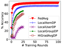
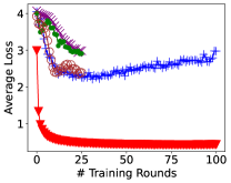
Shakespeare

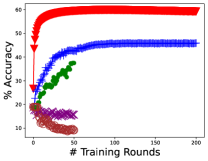
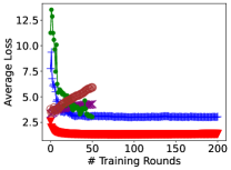
(a)                                                     

(b)

(c)                                                     

(d)

Figure 1. Average test accuracy and loss on the FEMNIST (a),(b) and Shakespeare (c),(d) datasets over training rounds for various algorithms. For DP guarantees: $\epsilon=4.0$ and $\delta=10^{-5}$ budgeted over all $100$ and $200$ training rounds for FEMNIST and Shakespeare respectively. Model performance for the subject level privacy algorithms is constrained by the limited number of training rounds ($25$ for FEMNIST, and $50$ for Shakespeare) permitted under the prescribed privacy budget.

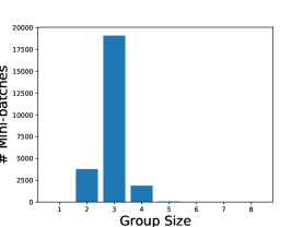
(a) FEMNIST

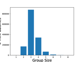
(b) Shakespeare

Figure 2. Number of mini-batches with subject group sizes over the entire training run for FEMNIST (a) and Shakespeare (b).

Figure 1 shows performance of the models trained using our algorithms. FedAvg performs the best since it does not incur any DP enforcement penalties. Item level privacy enforcement in LocalItemDP results in performance degradation of $8\%$ for FEMNIST and $22\%$ for Shakespeare. The utility cost of user level LDP in UserLDP is quite clear from the figure. This cost is also reflected in the relatively high observed loss for the respective model.  performs significantly better than UserLDP, but worse than LocalItemDP, by $15\%$ on FEMNIST, and $18\%$ on Shakespeare. The reason for ’s worse performance is clear from Figure 2(a) and (c): the group size for a mini-batch tends to be dominated by $3$ on both FEMNIST and Shakespeare, which cuts the privacy budget for these mini-batches by a factor of $3$, leading to greater Gaussian noise, which in turn leads to model performance degradation.

performs worse than  because we need to use the sampling fraction of largest cardinality subjects at federation users when calculating mini-batch noise scale (Theorem 3.7). This amounts to noise scale amplification by approximately an order of magnitude. This amplification is much higher for Shakespeare (with an average of $4,484$ data items per subject) by another order of magnitude, because of which ’s model’s utility is the worst. Moreover, privacy loss amplification due to horizontal composition limits the amount of training thereby further limiting model utility (in all our algorithms).

5.2. Effect of Subject Data Distribution

While evaluation of our algorithms using a uniform distribution of subject data among federation users is a good starting point, often times the data distribution is non-uniform in real world settings. To emulate varying subject data distributions, we conduct experiments on the FEMNIST dataset where subject data is distributed among federation users according to the power distribution

$$P(x;\alpha)=\alpha x^{\alpha-1},0\leq x\leq 1,\alpha>0$$

Figure 3 shows performance of the models trained using our algorithms over varying subject data distributions of FEMNIST. As expected, different data distributions clearly do not significantly affect FedAvg, LocalItemDP, and User-Local-SGD. However, performance of the model trained using  degrades noticeably as the unevenness of data distribution increases, resulting in test accuracy under $50\%$ for $\alpha=16$. This degradation is singularly attributable to growth in subject group size per mini-batch – the average group size per mini-batch ranges from $3$ when $\alpha=2$ to $6$ when $\alpha=16$. This increase in group size significantly reduces the privacy budget leading to increase in Gaussian noise that restricts test accuracy. On the other hand, though ’s model utility is much lower than that of ’s, it appears to be much more resilient to non-uniform subject data distributions among federation users up to $\alpha=8$, and therafter drops noticeably at $\alpha=16$.

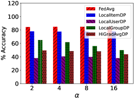
Figure 3. Model performance over FEMNIST dataset of our algorithms over different subject data distributions dictated by the parameter $\alpha$ of the power distribution.

6. Conclusion

While various prior works on privacy in FL have explored DP guarantees at the user and item levels (Liu et al.,, 2020; McMahan et al.,, 2018), to the best of our knowledge, no prior work has studied subject level granularity for privacy in the FL setting. In this paper, we presented a formal definition of subject level DP. We also presented three novel FL training algorithms that guarantee subject level DP by either enforcing user level LDP (UserLDP), local group DP (), or by applying hierarchical gradient averaging to obfuscate a subject’s contribution to mini-batch gradients (). Our formal analysis over convex loss functions shows that all our algorithms affect utility loss in interesting ways, with  incurring lower utility loss than UserLDP and . Our empirical evaluation on the FEMNIST and Shakespeare datasets aligns with our formal analysis showing that while both UserLDP and  can significantly degrade model performance,  tends to incur much less loss in model performance compared to LocalItemDP, an algorithm that provides a weaker item level privacy guarantee. We also observe an interesting new aspect of horizontal composition of privacy loss for subject level privacy in FL that results in model performance degradation. Both our formal and empirical analysis demonstrate that there remains significant room for model utility improvements in algorithms that guarantee subject level DP in FL.

Appendix A Additional Proofs

The following theorem is a restatement of Theorem 3.2 and, in our notation, of Theorem $2.2$ and the associated footnote $1$ from Dwork and Roth (Dwork & Roth,, 2014, §2.3):

Theorem A.1.

Any ($\varepsilon,\delta$)-differentially private randomized algorithm $\mathcal{A}:\mathcal{D}\rightarrow\mathcal{R}$ is ($k\varepsilon,ke^{(k-1)\varepsilon}\delta$)-differentially private for groups of size $k\geq 2$. That is, for all $D,D^{\prime}\in\mathcal{D}$ such that $D$ and $D^{\prime}$ differ in at most $k$ data items, and for all $S\subseteq\mathcal{R}$,

$$\mathrm{Pr}[\mathcal{A}(D)\in S] \leq e^{k\varepsilon}\mathrm{Pr}[\mathcal{A}(D^{\prime})\in S]+{\displaystyle{e^{k\varepsilon}-1\over e^{\varepsilon}-1}}\delta$$

$$\leq e^{k\varepsilon}\mathrm{Pr}[\mathcal{A}(D^{\prime})\in S]+ke^{(k-1)\varepsilon}\delta$$

$$< e^{k\varepsilon}\mathrm{Pr}[\mathcal{A}(D^{\prime})\in S]+ke^{k\varepsilon}\delta$$

Proof.

Suppose that $D$ and $D^{\prime}$ differ in exactly $k$ data items. Choose any order for these items and call them $d_{1},d_{2},\ldots,d_{k}$. Let $D_{0},D_{1},\ldots,D_{k}$ be $k+1$ datasets such that $D_{0}=D$, and $D_{k}=D^{\prime}$, and for all $1\leq i\leq k$ it holds that $D_{i-1}$ and $D_{i}$ differ by exactly one data item, namely $d_{i}$. It follows that:

$$\begin{array}[]{lll}\hbox to0.0pt{$\mathrm{Pr}[\mathcal{A}(D_{0})\in S]$\hss\hss}\\ &\leq&e^{\varepsilon}\mathrm{Pr}[\mathcal{A}(D_{1})\in S]+\delta\\ &\leq&e^{\varepsilon}(e^{\varepsilon}\mathrm{Pr}[\mathcal{A}(D_{2})\in S]+\delta)+\delta\\ &\leq&e^{\varepsilon}(e^{\varepsilon}(e^{\varepsilon}\mathrm{Pr}[\mathcal{A}(D_{3})\in S]+\delta)+\delta)+\delta\\ &\leq&\cdots\\ &\leq&e^{\varepsilon}(e^{\varepsilon}(e^{\varepsilon}\cdots(e^{\varepsilon}\mathrm{Pr}[\mathcal{A}(D_{k})\in S]+\delta)\cdots+\delta)+\delta)+\delta\\ &\leq&e^{k\varepsilon}\mathrm{Pr}[\mathcal{A}(D^{\prime})\in S]+{\displaystyle\left(\sum_{0\leq i\leq k-1}e^{i\varepsilon}\right)}\delta\\ &=&e^{k\varepsilon}\mathrm{Pr}[\mathcal{A}(D^{\prime})\in S]+{\displaystyle{e^{k\varepsilon}-1\over e^{\varepsilon}-1}}\delta\end{array}$$

This is the tightest possible bound using this proof technique (also presented as Lemma $1$ in (Jagielski et al.,, 2020)). However, the expression ${e^{k\varepsilon}-1\over e^{\varepsilon}-1}\delta$ can be unwieldy for some purposes. Other authors (Dwork & Roth,, 2014; Vadhan,, 2017) state this theorem with a slightly larger value than necessary, perhaps for the sake of conciseness: because $e^{i\varepsilon}\leq e^{(k-1)\varepsilon}$ for any $i\leq k-1$, $\left(\sum_{0\leq i\leq k-1}e^{i\varepsilon}\right)\delta\leq\left(\sum_{0\leq i\leq k-1}e^{(k-1)\varepsilon}\right)\delta=ke^{(k-1)\varepsilon}\delta$ (Dwork & Roth,, 2014) (equality with ${e^{k\varepsilon}-1\over e^{\varepsilon}-1}\delta$ holds only when $k=1$). Sometimes $ke^{(k-1)\varepsilon}\delta$ is further simplified to $ke^{k\varepsilon}\delta$ (Vadhan,, 2017), which is strictly larger for all $k\geq 1$.

Because all four of the expressions $e^{k\varepsilon}$, ${e^{k\varepsilon}-1\over e^{\varepsilon}-1}\delta$, $ke^{(k-1)\varepsilon}\delta$, and $ke^{k\varepsilon}\delta$ decrease (strictly) monotonically as $k$ decreases, the same statements apply even if $D$ and $D^{\prime}$ differ in fewer than $k$ data items. Thus one can say that $\mathcal{A}$ is either ($k\varepsilon,{e^{k\varepsilon}-1\over e^{\varepsilon}-1}\delta$)-differentially private, ($k\varepsilon,ke^{(k-1)\varepsilon}\delta$)-differentially private, or even ($k\varepsilon,ke^{k\varepsilon}\delta$)-differentially private for groups of size $k$; the first of these three statements is the tightest bound on the failure probability. ∎

Theorem A.2 (Same as Theorem 3.11).

UserLDP with parameter updates satisfying Equation 6 as observed by the federation server in a training round, enforces user level ($\varepsilon$,$\delta$)-local differential privacy provided the noise parameter $\sigma$ satisfies the inequality from Theorem 3.10, and the following inequality

$$\sigma>\frac{1}{\sqrt{2\pi}\varepsilon\delta e^{\varepsilon}}$$

Proof.

Let $O(u_{1})$ and $O(u_{2})$ be the norms of the unperturbed outputs of a training round for users $u_{1}$ and $u_{2}$ respectively.

Assuming w.l.o.g. training for $T$ mini-batches per training round at $u_{1}$ and $u_{2}$, from Lemma 3.9 we get

$$O(u_{1})\leq\eta TC$$

$$O(u_{2})\leq\eta TC$$

Now the privacy loss random variable of interest is

$$\bigg{|}log\frac{\mathcal{P}[F_{l}(D_{u_{1}}]=s}{\mathcal{P}[F_{l}(D_{u_{2}})]=s}\bigg{|}=\bigg{\rvert}log\frac{exp(\frac{-1}{2\sigma^{2}}O(u_{1})^{2})}{exp(\frac{-1}{2\sigma^{2}}O(u_{2})^{2})}\bigg{\rvert}$$

$$=\bigg{\rvert}log\ exp(\frac{-1}{2\sigma^{2}}(O(u_{2})^{2}-O(u_{1})^{2}))\bigg{\rvert}$$

$$=\frac{1}{2\sigma^{2}}|O(u_{2})^{2}-O(u_{1})^{2}|$$

This quantity is upper bounded by $\varepsilon$ if

$$|O(u_{2})^{2}-O(u_{1})^{2}|\leq 2\varepsilon\sigma^{2}$$

For the failure probability bound $\delta$ we need

$$\mathcal{P}[|O(u_{2})^{2}-O(u_{1})^{2}|\geq 2\varepsilon\sigma^{2}]<\delta$$

We use the tail bound for Gaussian distributions

$$\mathcal{P}[x>t]\leq\frac{\sigma}{\sqrt{2\pi}}\frac{1}{t}exp(\frac{-t^{2}}{2\sigma^{2}})$$

Because we are concerned with just $|O(u_{2})^{2}-O(u_{1})^{2}|$ we will find $\sigma$ such that

$$\frac{\sigma}{\sqrt{2\pi}}\frac{1}{t}exp(\frac{-t^{2}}{2\sigma^{2}})<\frac{\delta}{2}$$

Substituting $t=2\varepsilon\sigma^{2}$ we get

$$\frac{\sigma}{\sqrt{2\pi}}\frac{1}{2\varepsilon\sigma^{2}}exp(\frac{-2\varepsilon\sigma^{2}}{2\sigma^{2}})<\frac{\delta}{2}$$

which resolves to

$$\sigma>\frac{1}{\sqrt{2\pi}\varepsilon\delta e^{\varepsilon}}$$

∎

Theorem A.3 (Same as Theorem 3.12).

Given a FL training algorithm $\mathcal{F}=(\mathcal{F}_{l},\mathcal{F}_{g})$, in the most general case where a subject’s data resides in the private datasets of multiple federation users $u_{i}$, the aggregation algorithm $\mathcal{F}_{g}$ adaptively composes subject level privacy losses incurred by $\mathcal{F}_{l}$ at each federation user.

Proof.

Assume two distinct users $u_{1}$ and $u_{2}$ in a federation that host private data items of subject $s$. Let $\varepsilon_{1}$ and $\varepsilon_{2}$ be the respective subject privacy losses incurred by the two users during a training round.

It is straightforward to see that, in the worst case, data items of $s$ at users $u_{1}$ and $u_{2}$ can affect disjoint parameters in $\mathcal{M}$. Thus parameter averaging done by $\mathcal{F}_{g}$ simply results in summation and scaling of these disjoint parameter updates. As a result, the privacy losses, $\varepsilon_{1}$ and $\varepsilon_{2}$ incurred by $u_{1}$ and $u_{2}$ respectively are retained to their entirety by $\mathcal{F}_{g}$. In other words, privacy losses incurred for subject $s$ at users $u_{1}$ and $u_{2}$ compose adaptively. ∎

Theorem A.4 (Same as Theorem 3.13).

Consider a FL training algorithm $\mathcal{F}=(\mathcal{F}_{l},\mathcal{F}_{g})$ that samples $s$ users per training round, and trains the model $\mathcal{M}$ for $R$ rounds. Let $\mathcal{F}_{l}$ at each participating user, over the aggregate of $R$ training rounds, locally enforce subject level ($\varepsilon$,$\delta$)-DP. Then $\mathcal{F}$ globally enforces the same subject level ($\varepsilon$,$\delta$)-DP guarantee by training for $\frac{R}{\sqrt{s}}$ rounds.

Proof.

The proof of training round constraints on horizontal composition can be broken down into two cases: First, each user in the federation locally trains for exactly $T$ mini-batches per training round, with exactly the same mini-batch sampling probability $q$. Since horizontal composition is equivalent to adaptive composition in the worst case, the moments accountant method shows us that the resulting algorithm will be $(O(q\varepsilon\sqrt{TRs}),\delta)$-differentially private. To compensate for the $\sqrt{s}$ factor scaling of the privacy loss, $\mathcal{F}$ can be executed for $\frac{R}{\sqrt{s}}$ training rounds, yielding a $(O(q\varepsilon\sqrt{TR}),\delta)$-differentially private algorithm.

In the second case, each user $u_{i}$ may train for a unique number of mini-batches per training round, with a unique mini-batch sampling probability dictated by $u_{i}$’s private dataset. Let $T_{1},T_{2},...,T_{s}$, and $q_{1},q_{2},...,q_{s}$ be the number of mini-batches per training round and mini-batch sampling fraction for the sampled users $u_{1},u_{2},...,u_{s}$ respectively.

All our algorithms 3, 1, and 2 locally enforce subject level ($O(q_{i}\varepsilon\sqrt{T_{i}R})$,$\delta$)-DP at each user $u_{i}$. Privacy enforcement is done independently at each federation user $u_{i}$. Furthermore, note that the privacy loss is uniformly apportioned among training rounds. Let $\mathcal{E}=O(q_{i}\varepsilon\sqrt{T_{i}R})$. Note that $\mathcal{E}$ is identical for each user $u_{i}$ in the federation. Thus if $\mathcal{E}$ is the total privacy loss budget over $R$ training rounds, a sampled user incurs $\varepsilon_{r}=\mathcal{E}/R$ privacy loss in a single training round $r$. Similarly, each of the $s$ sampled users in round $r$ incurs identical privacy loss $\varepsilon_{r}$ despite having different mini-batches per training round $T_{i}$ and mini-batch sampling probabilities $q_{i}$s. As noted earlier, these privacy losses compose horizontally (adaptively) via $\mathcal{F}_{g}$ over $s$ users, leading to privacy loss amplification by a factor of $\sqrt{s}$ as per the moments accountant method. Given a fixed privacy loss budget $\mathcal{E}$, to compensate for this privacy loss amplification, $\mathcal{F}$ can be executed for $\frac{R}{\sqrt{s}}$ training rounds. ∎

References

- Abadi et al., (2016) Abadi, Martin, Chu, Andy, Goodfellow, Ian, McMahan, H. Brendan, Mironov, Ilya, Talwar, Kunal, & Zhang, Li. 2016. Deep Learning with Differential Privacy. Pages 308–318 of: Proceedings of the 2016 ACM SIGSAC Conference on Computer and Communications Security.
- Bassily et al., (2014) Bassily, Raef, Smith, Adam D., & Thakurta, Abhradeep. 2014. Private Empirical Risk Minimization: Efficient Algorithms and Tight Error Bounds. Pages 464–473 of: 55th IEEE Annual Symposium on Foundations of Computer Science. IEEE Computer Society.
- Bassily et al., (2019) Bassily, Raef, Feldman, Vitaly, Talwar, Kunal, & Thakurta, Abhradeep. 2019. Private Stochastic Convex Optimization with Optimal Rates. CoRR, abs/1908.09970.
- Bonawitz et al., (2019) Bonawitz, Keith, Eichner, Hubert, Grieskamp, Wolfgang, Huba, Dzmitry, Ingerman, Alex, Ivanov, Vladimir, Kiddon, Chloé, Konecný, Jakub, Mazzocchi, Stefano, McMahan, H. Brendan, Overveldt, Timon Van, Petrou, David, Ramage, Daniel, & Roselander, Jason. 2019. Towards Federated Learning at Scale: System Design. CoRR, abs/1902.01046.
- Bousquet & Elisseeff, (2002) Bousquet, Olivier, & Elisseeff, André. 2002. Stability and Generalization. Journal of Machine Learning Research, 2, 499–526.
- Caldas et al., (2018) Caldas, Sebastian, Wu, Peter, Li, Tian, Konečný, Jakub, McMahan, H. Brendan, Smith, Virginia, & Talwalkar, Ameet. 2018. LEAF: A Benchmark for Federated Settings. CoRR, abs/1812.01097.
- Chaudhuri et al., (2011) Chaudhuri, Kamalika, Monteleoni, Claire, & Sarwate, Anand D. 2011. Differentially Private Empirical Risk Minimization. The Journal of Machine Learning Research, 12(July), 1069–1109.
- Differential Privacy Team, (2017) Differential Privacy Team, Apple. 2017. Learning with Privacy at Scale. Machine Learning, Journal, 1(8), 1–25.
- Dong et al., (2019) Dong, Jinshuo, Roth, Aaron, & Su, Weijie J. 2019. Gaussian Differential Privacy. CoRR, abs/1905.02383.
- Duchi et al., (2013) Duchi, John C., Jordan, Michael I., & Wainwright, Martin J. 2013. Local Privacy and Statistical Minimax Rates. CoRR, abs/1302.3203.
- Dwork & Roth, (2014) Dwork, Cynthia, & Roth, Aaron. 2014. The Algorithmic Foundations of Differential Privacy. Foundations and Trends in Theoretical Computer Science, 9(3–4), 211–407.
- Dwork et al., (2006) Dwork, Cynthia, McSherry, Frank, Nissim, Kobbi, & Smith, Adam. 2006. Calibrating Noise to Sensitivity in Private Data Analysis. Pages 265–284 of: Proceedings of the Third Conference on Theory of Cryptography. TCC’06.
- Dwork et al., (2010) Dwork, Cynthia, Rothblum, Guy N., & Vadhan, Salil P. 2010. Boosting and Differential Privacy. Pages 51–60 of: 51th Annual IEEE Symposium on Foundations of Computer Science, FOCS.
- Iyengar et al., (2019) Iyengar, Roger, Near, Joseph P., Song, Dawn, Thakkar, Om, Thakurta, Abhradeep, & Wang, Lun. 2019. Towards Practical Differentially Private Convex Optimization. Pages 299–316 of: 2019 IEEE Symposium on Security and Privacy. IEEE.
- Jagielski et al., (2020) Jagielski, Matthew, Ullman, Jonathan R., & Oprea, Alina. 2020. Auditing Differentially Private Machine Learning: How Private is Private SGD? In: Advances in Neural Information Processing Systems 33: Annual Conference on Neural Information Processing Systems 2020.
- Kairouz et al., (2019) Kairouz, Peter, McMahan, H. Brendan, Avent, Brendan, Bellet, Aurélien, Bennis, Mehdi, Bhagoji, Arjun Nitin, Bonawitz, Keith, Charles, Zachary, Cormode, Graham, Cummings, Rachel, D’Oliveira, Rafael G. L., Rouayheb, Salim El, Evans, David, Gardner, Josh, Garrett, Zachary, Gascón, Adrià, Ghazi, Badih, Gibbons, Phillip B., Gruteser, Marco, Harchaoui, Zaïd, He, Chaoyang, He, Lie, Huo, Zhouyuan, Hutchinson, Ben, Hsu, Justin, Jaggi, Martin, Javidi, Tara, Joshi, Gauri, Khodak, Mikhail, Konecný, Jakub, Korolova, Aleksandra, Koushanfar, Farinaz, Koyejo, Sanmi, Lepoint, Tancrède, Liu, Yang, Mittal, Prateek, Mohri, Mehryar, Nock, Richard, Özgür, Ayfer, Pagh, Rasmus, Raykova, Mariana, Qi, Hang, Ramage, Daniel, Raskar, Ramesh, Song, Dawn, Song, Weikang, Stich, Sebastian U., Sun, Ziteng, Suresh, Ananda Theertha, Tramèr, Florian, Vepakomma, Praneeth, Wang, Jianyu, Xiong, Li, Xu, Zheng, Yang, Qiang, Yu, Felix X., Yu, Han, & Zhao, Sen. 2019. Advances and Open Problems in Federated Learning. CoRR, abs/1912.04977.
- Kasiviswanathan et al., (2008) Kasiviswanathan, Shiva Prasad, Lee, Homin K., Nissim, Kobbi, Raskhodnikova, Sofya, & Smith, Adam D. 2008. What Can We Learn Privately? CoRR, abs/0803.0924.
- Kifer et al., (2012) Kifer, Daniel, Smith, Adam D., & Thakurta, Abhradeep. 2012. Private Convex Optimization for Empirical Risk Minimization with Applications to High-dimensional Regression. Pages 25.1–25.40 of: The 25th Annual Conference on Learning Theory, vol. 23.
- Konecný et al., (2015) Konecný, Jakub, McMahan, Brendan, & Ramage, Daniel. 2015. Federated Optimization: Distributed Optimization Beyond the Datacenter. CoRR, abs/1511.03575.
- Levy et al., (2021) Levy, Daniel, Sun, Ziteng, Amin, Kareem, Kale, Satyen, Kulesza, Alex, Mohri, Mehryar, & Suresh, Ananda Theertha. 2021. Learning with User-Level Privacy. CoRR, abs/2102.11845.
- Liu et al., (2020) Liu, Yuhan, Suresh, Ananda Theertha, Yu, Felix X., Kumar, Sanjiv, & Riley, Michael. 2020. Learning discrete distributions: user vs item-level privacy. CoRR, abs/2007.13660.
- McMahan et al., (2018) McMahan, H. Brendan, Ramage, Daniel, Talwar, Kunal, & Zhang, Li. 2018. Learning Differentially Private Recurrent Language Models. In: 6th International Conference on Learning Representations, ICLR 2018.
- McSherry, (2009) McSherry, Frank. 2009. Privacy integrated queries: an extensible platform for privacy-preserving data analysis. Pages 19–30 of: Proceedings of the ACM SIGMOD International Conference on Management of Data.
- Mironov, (2017) Mironov, Ilya. 2017. Renyi Differential Privacy. CoRR, abs/1702.07476.
- Shalev-Shwartz & Ben-David, (2014) Shalev-Shwartz, Shai, & Ben-David, Shai. 2014. Understanding machine learning: From theory to algorithms. Cambridge University Press.
- Song et al., (2013) Song, Shuang, Chaudhuri, Kamalika, & Sarwate, Anand D. 2013. Stochastic gradient descent with differentially private updates. Pages 245–248 of: IEEE Global Conference on Signal and Information Processing.
- Talwar et al., (2015) Talwar, Kunal, Thakurta, Abhradeep, & Zhang, Li. 2015. Nearly Optimal Private LASSO. Pages 3025–3033 of: Annual Conference on Neural Information Processing Systems.
- Thakurta & Smith, (2013) Thakurta, Abhradeep, & Smith, Adam D. 2013. Differentially Private Feature Selection via Stability Arguments, and the Robustness of the Lasso. Pages 819–850 of: COLT 2013 - The 26th Annual Conference on Learning Theory, vol. 30.
- Truex et al., (2020) Truex, Stacey, Liu, Ling, Chow, Ka Ho, Gursoy, Mehmet Emre, & Wei, Wenqi. 2020. LDP-Fed: Federated Learning with Local Differential Privacy. Pages 61–66 of: Proceedings of the 3rd International Workshop on Edge Systems, Analytics and Networking, EdgeSys@EuroSys 2020, Heraklion, Greece, April 27, 2020. ACM.
- Vadhan, (2017) Vadhan, Salil P. 2017. The Complexity of Differential Privacy. Pages 347–450 of: Tutorials on the Foundations of Cryptography. Springer International Publishing.
- Wang et al., (2018) Wang, Di, Ye, Minwei, & Xu, Jinhui. 2018. Differentially Private Empirical Risk Minimization Revisited: Faster and More General. CoRR, abs/1802.05251.
- Wang et al., (2021) Wang, Jianyu, Charles, Zachary, Xu, Zheng, Joshi, Gauri, McMahan, H. Brendan, y Arcas, Blaise Aguera, Al-Shedivat, Maruan, Andrew, Galen, Avestimehr, Salman, Daly, Katharine, Data, Deepesh, Diggavi, Suhas, Eichner, Hubert, Gadhikar, Advait, Garrett, Zachary, Girgis, Antonious M., Hanzely, Filip, Hard, Andrew, He, Chaoyang, Horvath, Samuel, Huo, Zhouyuan, Ingerman, Alex, Jaggi, Martin, Javidi, Tara, Kairouz, Peter, Kale, Satyen, Karimireddy, Sai Praneeth, Konecny, Jakub, Koyejo, Sanmi, Li, Tian, Liu, Luyang, Mohri, Mehryar, Qi, Hang, Reddi, Sashank J., Richtarik, Peter, Singhal, Karan, Smith, Virginia, Soltanolkotabi, Mahdi, Song, Weikang, Suresh, Ananda Theertha, Stich, Sebastian U., Talwalkar, Ameet, Wang, Hongyi, Woodworth, Blake, Wu, Shanshan, Yu, Felix X., Yuan, Honglin, Zaheer, Manzil, Zhang, Mi, Zhang, Tong, Zheng, Chunxiang, Zhu, Chen, & Zhu, Wennan. 2021. A Field Guide to Federated Optimization.
- Wang et al., (2019) Wang, Yu-Xiang, Balle, Borja, & Kasiviswanathan, Shiva Prasad. 2019. Subsampled Renyi Differential Privacy and Analytical Moments Accountant. Pages 1226–1235 of: The 22nd International Conference on Artificial Intelligence and Statistics. Proceedings of Machine Learning Research, vol. 89.
- Warner, (1965) Warner, Stanley L. 1965. Randomized response: A survey tech-nique for eliminating evasive answer bias. Journal ofthe American Statistical Association, 60(309), 63–69.