FedPop: A Bayesian Approach for Personalised Federated Learning

Abstract

Personalised federated learning (FL) aims at collaboratively learning a machine learning model tailored for each client. Albeit promising advances have been made in this direction, most of existing approaches do not allow for uncertainty quantification which is crucial in many applications. In addition, personalisation in the cross-silo and cross-device setting still involves important issues, especially for new clients or those having small number of observations. This paper aims at filling these gaps. To this end, we propose a novel methodology coined FedPop by recasting personalised FL into the population modeling paradigm where clients’ models involve fixed common population parameters and random effects, aiming at explaining data heterogeneity. To derive convergence guarantees for our scheme, we introduce a new class of federated stochastic optimisation algorithms which relies on Markov chain Monte Carlo methods. Compared to existing personalised FL methods, the proposed methodology has important benefits: it is robust to client drift, practical for inference on new clients, and above all, enables uncertainty quantification under mild computational and memory overheads. We provide non-asymptotic convergence guarantees for the proposed algorithms and illustrate their performances on various personalised federated learning tasks.

1 Introduction

Federated learning (FL) is a recent machine learning paradigm in which distributed clients holding siloed data collaborate in solving a learning problem, usually under the coordination of a central server (Wang et al., 2021; Kairouz et al., 2021). One of the main focus of FL is on so-called cross-device applications where a large number of personal electronic devices such as mobile phones, wearable devices or home assistants collect and store data at the edges of a decentralised network (McMahan et al., 2017).

While standard FL methods (McMahan et al., 2017; Alistarh et al., 2017; Karimireddy et al., 2020; Horváth et al., 2019; Li et al., 2020) have focused on training a global model that can be applied to individual agents, the relevance of such inferences has recently been questioned due to statistical heterogeneity between clients. Indeed, the considered common model may not generalise well on a client with a local data distribution that differs significantly from the global data distribution, especially if that client has not participated in the training process. In fact, it might even be better for such clients to derive a local model from their own data set. To circumvent these issues, a number of personalised federated learning approaches have recently been proposed, that use local models to fit client-specific data distribution while capturing some shared knowledge via a federated scheme (Tan et al., 2022). Personalisation has previously been approached using multi-task learning (Smith et al., 2017), meta-learning (Jiang et al., 2019; Khodak et al., 2019), client clustering (Briggs et al., 2020), data interpolation (Mansour et al., 2020), model interpolation (Hanzely and Richtárik, 2020; Hanzely et al., 2020) or partially local models (Singhal et al., 2021; Collins et al., 2021). While these methodologies are promising, they only partially solve the personalisation problem in highly heterogeneous federated settings and have no means of quantifying uncertainty. In addition, cross-device FL also faces other important challenges such as (extreme) partial device participation, small local data sets, limited upload bandwidth and device capabilities (Kairouz et al., 2021). Addressing these problems for personalised FL requires new paradigms regarding how model knowledge is shared and personalisation is performed locally.

Proposed Approach. In this paper, we adopt a novel perspective to model the problem of personalised FL. This paradigm, called mixed-effects modeling (also known as multi-level or population approach) is widely used to analyse data that have a clustered or nested structure, as in medical or biological research where multiple observations per patient are available (Gelman and Hill, 2007; Long, 2011; Lavielle, 2014). Although the hierarchical structure of FL has already been noted (Plassier et al., 2021; Grant et al., 2018; Hong et al., 2022), the mixed-effects paradigm has interestingly never been considered. Leveraging this framework, we develop a new model for personalised FL called FedPop and propose an efficient computational solution to perform inference under this model. More precisely, we introduce a novel class of federated stochastic approximation algorithms based on parallel Markov Chain Monte Carlo (MCMC) methods. In the proposed framework, we also pay special attention to the cross-device setting by taking into account partial client participation, and by addressing the communication bottleneck with both multiple local updates and the use of lossy compression operators.

Benefits. Up to the authors’ knowledge, FedPop is the first personalised FL approach that allows cheap uncertainty quantification with a theoretically-grounded methodology. The proposed framework also comes with other interesting properties. First, in contrast to most of personalised FL methods that only consider “fixed-effects” models (Collins et al., 2021; Hanzely et al., 2021; Smith et al., 2017), FedPop provides credibility information (via credibility regions) and allows more accurate inference for clients with small and heterogeneous local data via partial pooling (Gelman and Hill, 2007). In addition, inference for new clients which did not participate in the training phase can be easily performed by sampling from the prior over the local random effects. Second, contrary to existing Bayesian FL approaches that aim to provide credibility information by sampling from a target posterior distribution (Hong et al., 2022; Yoon et al., 2018; Vono et al., 2022; El Mekkaoui et al., 2021), FedPop allows to perform personalisation and cheaper on-device uncertainty quantification taking an empirical Bayes prediction approach. Finally, an important benefit of FedPop is its ability to allow for multiple local updates without suffering from the client-drift phenomenon (Karimireddy et al., 2020).

Outline and Contributions. Our contributions are fourfold. First, in Section 2, we propose a novel probabilistic methodology, which we call FedPop, to address personalisation under the cross-device FL paradigm. To perform efficient inference under this model, we introduce a general class of stochastic approximation algorithms based on MCMC. Second, we provide in Section 3 non-asymptotic convergence guarantees for the proposed methodology. Then, we perform in Section 4 a comparison between the proposed approach and exisiting works. Finally, we illustrate in Section 5 the benefits of our methodology on several federated learning benchmarks involving both synthetic and real data.

2 Proposed Approach

In this section, we present the statistical estimation problem we are considering and the proposed methodology called FedPop to address it.

Problem Formulation. We are interested in the cross-device FL setting involving a large number $b\in\mathbb{N}^{*}$ of clients, potentially unreliable i.e. not necessarily available at each communication round. These clients are assumed to own sensitive local data sets $\{\mathrm{D}_{i}\}_{i\in[b]}$. In this framework, we aim to make both uncertainty quantification and personalised statistical inference by learning a local model tailored to each client. To this end, and inspired by the population approach used in the biological and physical sciences (Lavielle, 2014), we consider mixed-effects modeling for each client leading to the local marginal likelihood function defined, for any $i\in[b]$, by

$$p({\textstyle{\mathrm{D}_{i}\mid\phi,\beta}})=\int_{\mathbb{R}^{d}}p({\textstyle{\mathrm{D}_{i}\mid\phi\,,z^{(i)}}})p({\textstyle{z^{(i)}\mid\beta}})\mathrm{d}z^{(i)}\,,$$ (1)

where $\phi\in\Phi\subseteq\mathbb{R}^{d_{\Phi}}$ stands for a fixed effect and $\{z^{(i)}\}_{i\in[b]}\in\mathsf{Z}$, $\mathsf{Z}=\prod_{i=1}^{b}\mathbb{R}^{d}$, represent random effects aimed at explaining statistical heterogeneity between local data sets $\{\mathrm{D}_{i}\}_{i\in[b]}$.

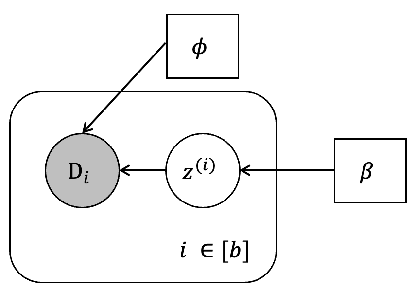
Figure 1: DAG for FedPop.

The objective of the fixed (i.e. constant across all clients) part is to capture a common representation (e.g. same features across different classes of images) while the random part, which is typically low-dimensional, performs personalisation and is assumed to be drawn from a population prior whose variance aims at modeling data heterogeneity.

Figure 1 illustrates this statistical framework, referred to as FedPop, by showing its directed acyclic graph (DAG) where grey-filled shapes indicate observed variables, white-filled shapes unknown variables and squared shapes variables to be estimated.

When the size of the local data set $\mathrm{D}_{i}$ is small, this common prior leverages information from other clients to limit the risk of overfitting and is often called partial pooling in the multi-level statistical literature (Gelman and Hill, 2007, Section 12). Examples of model architectures involving $\phi$ and $\{z^{(i)}\}_{i\in[b]}$ include for instance composition-based architectures $p({\textstyle{\mathrm{D}_{i}\mid\phi,z^{(i)}}})=p({\textstyle{\mathrm{D}_{i}\mid h_{\phi}\circ h_{z^{(i)}}}})$ where $h_{\phi}$ and $h_{z^{(i)}}$ are two neural networks (Collins et al., 2021; Arivazhagan et al., 2019). For the sake of generality, we propose to adopt a flexible energy-based prior distribution of the form for each $i\in[b]$,

$$p({\textstyle{z^{(i)}\mid\beta}})=\frac{1}{Z(\beta)}\exp\left\{{-E(z^{(i)};\beta)}\right\}\,,\text{ where $Z(\beta)=\int_{\mathbb{R}^{d}}\exp\left\{{-E(z^{(i)};\beta)}\right\}\mathrm{d}z^{(i)}$ }\,.$$ (2)

Here, $Z(\beta)$ is a normalising constant and $E(\cdot;\beta)$ represents an energy function, typically a neural network, parameterised by a set of parameters $\beta\in\mathsf{B}\subseteq\mathbb{R}^{d_{\mathsf{B}}}$ (LeCun et al., 2006). This framework is particularly interesting in the cross-device setting where the number of clients $b$ is large as it allows for efficient enrichment of the model. However, in the case where $b$ is small, the inference of the parameter $\beta$ is difficult. In this situation, a more pragmatic solution is to consider a common prior for the local random effects $\{z^{(i)}\}_{i\in[b]}$ which is held fixed, i.e. $p({\textstyle{z^{(i)}\mid\beta}})\propto\exp\{-E(z^{(i)})\}$ for any $\beta\in\mathsf{B}$. Finally, for completeness, we allow the use of a prior model $p(\phi,\beta)$ for the hyperparameters $\{\phi,\beta\}$. Using Bayes’ rule (Robert, 2001) and by denoting $\mathrm{D}=\sqcup_{i=1}^{b}\mathrm{D}_{i}$ the global data set, the posterior distribution associated with these hyperparameters admits a probability density function which can be written as

$$p\left({\phi,\beta\mid\mathrm{D}}\right)\propto p(\phi,\beta)\prod_{i=1}^{b}\left[{\int_{\mathbb{R}^{d}}p({\textstyle{\mathrm{D}_{i}\mid\phi,z^{(i)}}})p({\textstyle{z^{(i)}\mid\beta}})\mathrm{d}z^{(i)}}\right]\,.$$ (3)

Set $\theta=\{\phi,\beta\}\in\Theta$ with $\Theta=\Phi\times\mathsf{B}$. In the sequel, we will be interested in solving the maximum a posteriori problem given by

$$\theta^{\star} \in\operatorname*{arg\,max}_{\theta\in\Theta}\ \log p({\textstyle{\phi,\beta\mid\mathrm{D}}})\,,$$ (4)

$$\log p({\textstyle{\phi,\beta\mid\mathrm{D}}}) =\log p(\phi,\beta)+\sum_{i=1}^{b}\left[{\log\int_{\mathbb{R}^{d}}p({\textstyle{\mathrm{D}_{i}\mid\phi,z^{(i)}}})p({\textstyle{z^{(i)}\mid\beta}})\mathrm{d}z^{(i)}}\right]+C\,,$$ (5)

where $C\in\mathbb{R}$ is a constant independent of $\theta$. Once we have estimated $\theta^{\star}$, using an empirical Bayesian approach, we can perform “for free” on-device uncertainty quantification for each client $i\in[b]$ by sampling from the local posterior distribution $p(z^{(i)}\mid\mathrm{D}_{i},\phi^{\star},\beta^{\star})$, which is typically designed to be low-dimensional.

Algorithm. To solve the optimisation problem (4), we can either use an alternating maximisation algorithm or perform global maximisation over $\Theta$. Since the former approach requires more upload bandwidth, in this work we consider the second alternative which is more suitable for FL. The gradient of the objective function (5) being intractable, we propose to resort to the stochastic approximation framework (Robbins and Monro, 1951) which iteratively defines $(\phi_{k},\beta_{k})_{k\in\mathbb{N}}$, starting from any $(\phi_{0},\beta_{0})\in\Theta$, via the recursions for any $k\in\mathbb{N}$,

$$\beta_{k+1} =\Pi_{\mathsf{B}}\left({\beta_{k}+\eta_{k+1}^{(1)}\left[{\nabla_{\beta}\log p(\phi_{k},\beta_{k})+\sum_{i=1}^{b}\textsl{g}^{(i)}_{k}(\phi_{k},\beta_{k})}\right]}\right)\,,$$ (6)

$$\phi_{k+1} =\Pi_{\Phi}\left({\phi_{k}+\eta_{k+1}^{(2)}\left[{\nabla_{\phi}\log p(\phi_{k},\beta_{k})+\sum_{i=1}^{b}\textsl{h}^{(i)}_{k}(\phi_{k},\beta_{k})}\right]}\right)\,,$$ (7)

where $\Pi_{\mathsf{C}}$ denotes the projection onto $\mathsf{C}\in\{\Phi,\mathsf{B}\}$, $(\eta_{k}^{(1)},\eta_{k}^{(2)})_{k\in\mathbb{N}^{*}}$ are sequences of step-sizes, and $\{\textsl{g}^{(i)}_{k}\,:\,i\in[b]\,,k\in\mathbb{N}^{*}\}$ and $\{\textsl{h}^{(i)}_{k}\,:\,i\in[b]\,,k\in\mathbb{N}^{*}\}$ are estimators of the intractable gradients $(\phi,\beta)\mapsto\nabla_{\beta}\log p(\mathrm{D}_{i}\mid\phi,\beta)$ and $(\phi,\beta)\mapsto\nabla_{\phi}\log p(\mathrm{D}_{i}\mid\phi,\beta)$ at $(\phi_{k},\beta_{k})$, where $p(\mathrm{D}_{i}\mid\phi,\beta)$ is defined in (1) for any $i\in[b]$.

The choices of the estimators $\{\textsl{g}^{(i)}_{k}\,:\,i\in[b]\,,k\in\mathbb{N}^{*}\}$ and $\{\textsl{h}^{(i)}_{k}\,:\,i\in[b]\,,k\in\mathbb{N}^{*}\}$ are motivated by the Fisher identity. More precisely, under mild regularity assumptions, and using the Lebesgue dominated convergence theorem, we have for any, $(\phi,\beta)\in\Theta$, $i\in[b]$

$$\nabla_{\beta}\log p(\mathrm{D}_{i}\mid\phi,\beta) =\int_{\mathbb{R}^{d}}\left[{\nabla_{\beta}\log p({\textstyle{\mathrm{D}_{i},z^{(i)}\mid\phi,\beta}})}\right]p({\textstyle{z^{(i)}\mid\mathrm{D}_{i},\phi,\beta}})\mathrm{d}z^{(i)}\,,$$ (8)

$$\nabla_{\phi}\log p(\mathrm{D}_{i}\mid\phi,\beta) =\int_{\mathbb{R}^{d}}\left[{\nabla_{\phi}\log p({\textstyle{\mathrm{D}_{i},z^{(i)}\mid\phi,\beta}})}\right]p({\textstyle{z^{(i)}\mid\mathrm{D}_{i},\phi,\beta}})\mathrm{d}z^{(i)}\,,$$ (9)

which suggests to consider

$$\textsl{g}_{k}^{(i)}(\phi,\beta) =\frac{1}{M}\sum_{m=1}^{M}\nabla_{\beta}\log p({\textstyle{Z_{k}^{(i,m)}\mid\beta}})\,,$$ (10)

$$\textsl{h}_{k}^{(i)}(\phi,\beta) =\frac{1}{M}\sum_{m=1}^{M}\nabla_{\phi}\log p({\textstyle{\mathrm{D}_{i}\mid Z_{k}^{(i,m)},\phi}})\,,$$ (11)

where $M\in\mathbb{N}^{*}$ and $Z_{k}^{(i,1:M)}=(Z_{k}^{(i,m)})_{m\in[M]}$ are approximate samples from $p(z^{(i)}\mid\mathrm{D}_{i},\phi,\beta)$. More precisely, we consider a family $\{Q^{(i)}_{\gamma,\theta}:\gamma\in(0,\bar{\gamma}],\theta\in\Theta\}$ where for any step-size $\gamma$, $Q^{(i)}_{\gamma,\theta}$ is a Markov kernel which targets a close approximation of $p(z^{(i)}\mid\mathrm{D}_{i},\theta)$ with $\theta=\{\phi,\beta\}$. As an example, we can use overdamped Langevin dynamics (Roberts and Tweedie, 1996; Welling and Teh, 2011) to generate these samples. In this case, $Q^{(i)}_{\gamma,\theta}$ is associated with a Gaussian probability density function $q^{(i)}_{\gamma,\theta}(z^{(i)},\cdot)$ with mean $z^{(i)}-\gamma\nabla_{z}\log p(z^{(i)}\mid\mathrm{D}_{i},\theta)$ and variance $2\gamma\mathrm{I}_{d}$. Note that the number of Monte Carlo draws per iteration $k$ is considered constant here but we can easily generalise our scheme to the non-constant setting. In addition, our scheme can also be generalised by taking into account stochastic gradient estimators of (10) and (11). For the sake of simplicity, we present our approach with standard gradients.

In this framework, we present the main steps of the corresponding stochastic approximation algorithm, called FedSOUK, in Algorithm 1. Since we consider the cross-device federated setting, note that only a random subset $\mathsf{A}_{k+1}$ of active (i.e. available) clients communicates with the central server at each iteration $k\in\mathbb{N}$. In addition, due to limited upload bandwidth, the potentially high-dimensional gradient estimator (11) is compressed locally via an unbiased stochastic compression operator $\mathscr{C}_{k+1}$ before being sent to the central server (Alistarh et al., 2017; Philippenko and Dieuleveut, 2020).

Stateful and Stateless Versions. Depending on local memory constraints and the participation rate, we allow for a possible warm-start strategy across communication rounds to improve the convergence properties of the proposed algorithm so that the proposed algorithm becomes stateful, see steps $4-7$ in Algorithm 1. In cases the participation rate is very low (e.g. each client might only participates once to the training process), we replace this warm-start strategy by the initialisation $Z_{k}^{(i,0)}\sim p(\cdot\mid\beta_{k})$ for any $i\in[b]$ and $k\in\{0,\ldots,K-1\}$. This yields a stateless version of our algorithm more suitable to the cross-device setting. Obviously, compared to the previously proposed warm-start strategy, the performances of Algorithm 1 will be affected negatively if we are using the same number of local iterations $M$. We end up with an interesting trade-off between local computations and communication: if client-server communication is a bottleneck, the stateless version of the algorithm allows to reduce the communication overhead at the price of longer sampling procedures on each client. Such analyses will be illustrated empirically in Section 5.

Computation Complexity. Compared to standard FL methods, our approach has an additional computational cost on the client side associated with Monte Carlo approximations $\{I_{k}^{(i)}\}$ and $\{J_{k}^{(i)}\}$. In practice, this cost is negligible. Indeed, in our experiments, we found that using a small value of $M\in[1,10]$ was sufficient to obtain state-of-the-art results in terms of accuracy on the test dataset. We would like to emphasize that this additional computational cost has also two side advantages compared to existing FL approaches: (1) it allows us to communicate less frequently with the central server and (2) it allows us to converge faster when the number of local iterations increases since Monte Carlo approximation becomes better.

Communication Overhead. As pointed out in Table 1, our methodology FedPop improves upon existing FL approaches regarding the communication overhead. Indeed, FedPop offers the flexibility to use both compression for sending updates to the server, and multiple local steps to reduce the communication frequency. As such, depending on the bandwidth and local computational power, the practitioner can adapt the number of local iterations and the parameter of the compression operator. Up to our knowledge, this work is the first one combining compression and multiple local steps for personalised FL.

Robustness to client drift. For simplicity, we will take the example of FedSOUL (see Algorithm 1) which uses the Markov kernel associated with Langevin Monte Carlo to compute gradient estimates of the local marginal likelihood. However, our answer holds for general Markov kernels (adjusted or unadjusted). In this scenario, $M$ steps of Langevin Monte Carlo are performed on each device to draw samples $\{Z_{k}^{(i,m)}\}$ used to compute Monte Carlo estimates $\{I_{k}^{(i)}\}$ and $\{J_{k}^{(i)}\}$. Increasing the number of local steps $M$ does not slow down convergence but instead allows for more accurate Monte Carlo integration and hence better convergence properties. In contrast, the client drift phenomenon for classical FL approaches (e.g. FedAvg proposed in McMahan et al. (2017)) slows down convergence as the number of local iterations $M$ increases.

Simple inference on new clients. Typical personalized FL approaches such as DITTO or FedRep require additional local training for inference on new clients. In contrast, the proposed methodology FedPop allows for a cheaper two-step approach once we have estimated $\theta^{\star}=(\phi^{\star},\beta^{\star})$, as detailed below for a new client $b+1$ with feature vector $x$:

1. Sample $\{Z_{b+1}^{(l)}\}_{l\in[L]}$ in a i.i.d. manner.

2. Estimate the posterior predictive function by $p(\cdot\mid x)\approx L^{-1}\sum_{l=1}^{L}p(\cdot\mid\phi^{\star},Z_{b+1}^{(l)},x)$.

The prior $p(z_{b+1}\mid\beta^{\star})$ is typically chosen so that sampling is computationally cheap, e.g. a Gaussian with diagonal covariance matrix as in our experiments, see Section 5.

Algorithm 1 FL via Stochastic Optimisation using Unadjusted Kernel (FedSOUK)

1:Input: nb. outer iterations $K$, nb. local iterations $M$, Markov kernels $\{Q^{(i)}_{\gamma,\theta}\}_{\gamma,\theta,i}$, step-sizes $\{\eta_{k}^{(1)},\eta_{k}^{(2)}\}_{k\in[K],i\in[b]}$ and initial points $Z_{0}^{(0)}\in\mathbb{R}^{d}$, $\beta_{0}\in\mathsf{B}$ and $\phi_{0}\in\Phi$.

2:for $k=0$ to $K-1$ do

3:     Server sends $\{\beta_{k+1},\phi_{k+1}\}$ to clients belonging to $\mathsf{A}_{k+1}$.

4:     for $i\in\mathsf{A}_{k+1}$ // On active clients $\mathsf{A}_{k+1}$ do

5:          // Warm-start of the SA scheme if possible

6:         if $k\geq 1$ then

7:              Set $Z_{k}^{(i,0)}=Z_{k-1}^{(i,M)}$.

8:         end if

9:          // Computation of key quantities using MCMC

10:         for $m=0$ to $M-1$ do

11:              Draw $Z_{k}^{(i,m+1)}\sim Q^{(i)}_{\gamma,\theta_{k}}\left({Z_{k}^{(i,m)},\cdot}\right)$.

12:               // For Langevin dynamics

13:               // Draw $\xi_{k}^{(i,m+1)}\sim\mathrm{N}(0_{d},\mathrm{I}_{d})$.

14:               // Set $Z_{k}^{(i,m+1)}=Z_{k}^{(i,m)}+\gamma\nabla_{z}\log p(Z_{k}^{(i,m)}\mid\mathrm{D}_{i},\phi_{k},\beta_{k})+\sqrt{2\gamma}\xi_{k}^{(i,m+1)}$.

15:         end for

16:          // Communication with the server

17:         Set $I_{k}^{(i)}=\frac{1}{M}\sum_{m=1}^{M}\nabla_{\beta}\log p\left({Z_{k}^{(i,m)}\mid\beta_{k}}\right)$.

18:         Set $J_{k}^{(i)}=\frac{1}{M}\sum_{m=1}^{M}\nabla_{\phi}\log p\left({\mathrm{D}_{i}\mid Z_{k}^{(i,m)},\phi_{k}}\right)$.

19:         Send $I_{k}^{(i)}$ and $\mathscr{C}_{k+1}\left({J_{k}^{(i)}}\right)$ to the central server.

20:     end for

21:     Set $\beta_{k+1}=\Pi_{\mathsf{B}}\left({\beta_{k}+\eta_{k+1}^{(1)}\left[{\nabla_{\beta}\log p(\phi_{k},\beta_{k})+\frac{b}{|\mathsf{A}_{k+1}|}\sum_{i\in\mathsf{A}_{k+1}}I_{k}^{(i)}}\right]}\right)$.

22:     Set $\phi_{k+1}=\Pi_{\Phi}\left({\phi_{k}+\eta_{k+1}^{(2)}\left[{\nabla_{\phi}\log p(\phi_{k},\beta_{k})+\frac{b}{|\mathsf{A}_{k+1}|}\sum_{i\in\mathsf{A}_{k+1}}\mathscr{C}_{k+1}\left({J_{k}^{(i)}}\right)}\right]}\right)$.

23:end for

24:Output: $\{\phi_{K},\beta_{K}\}$ and samples $\{Z_{K-1}^{(1:b,m)}\}_{m=1}^{M}$.

3 Theoretical Guarantees

In this section, we present non-asymptotic convergence guarantees for Algorithm 1 when the family of Markov kernels $\{Q^{(i)}_{\gamma,\theta}:\gamma\in(0,\bar{\gamma}],\theta\in\Theta,i\in[b]\}$ is associated to unadjusted, i.e. without Metropolis acceptance step, overdamped Langevin dynamics (Durmus and Moulines, 2017; Dalalyan, 2017). The bounds we derive allow to showcase explicitly the impact of FL constraints, namely partial participation and compression. Results for general unadjusted Markov kernels are postponed to the supplement.

To show our theoretical results and resort to standard assumptions made in the stochastic approximation literature, we consider a minimisation problem and rewrite the opposite of the objective function (5) for any $\theta\in\Theta$ as

$$f(\theta)=b^{-1}\sum_{i=1}^{b}f_{i}(\theta)\,,\quad\text{where}\ f_{i}\left({\theta}\right)=-\log p(\phi,\beta)-b\log p\left({\mathrm{D}_{i}\mid\phi,\beta}\right)\,.$$ (12)

Non-Asymptotic Convergence Bounds. For the sake of better readability, we only detail in the main paper assumptions regarding the objective function, compression operators and the partial participation scenario. Technical assumptions related to the Markov kernels $\{Q^{(i)}_{\gamma,\theta}\}$ are postponed to the supplement. In spirit, we require, for any $i\in[b],\theta\in\Theta$ and $\gamma$, that $Q^{(i)}_{\gamma,\theta}$ satisfies some ergodic condition and can provide samples sufficiently close to the local posterior distribution $p(z^{(i)}\mid\mathrm{D}_{i},\theta)$. For the sake of simplicity, we also assume that for any $k\in\mathbb{N}^{*},\eta_{k}^{(1)}=\eta^{(2)}_{k}=\eta_{k}$, see Algorithm 1.

We make the following assumptions on $\Theta$ and the family of functions $\{f_{i}:i\in[b]\}$.

H 1.

$\Theta$ is convex, closed subset of $\mathbb{R}^{d_{\Theta}}$ and $\Theta\subset\mathrm{B}(0,R_{\Theta})$ for $R_{\Theta}>0$.

H 2.

For any $i\in[b]$, the following conditions hold.

1. The function $f_{i}$ defined in (S3) is convex.

2. There exist an open set $\mathsf{U}\in\mathbb{R}^{d_{\Theta}}$ and $L_{f}>0$ such that $\Theta\subset\mathsf{U}$, $f_{i}\in\mathrm{C}^{1}(\mathsf{U},\mathbb{R})$ and for any $\theta_{1},\theta_{2}\in\Theta$,

   $$\left\|{\nabla f_{i}(\theta_{2})-\nabla f_{i}(\theta_{1})}\right\|\leq L_{f}\left\|{\theta_{2}-\theta_{1}}\right\|\,.$$

The assumption below requires compression operators $\{\mathscr{C}_{k}\}_{k\in\mathbb{N}^{*}}$ to be unbiased and to have a bounded variance. Such an assumption is for instance verified by stochastic quantisation operators, see Alistarh et al. (2017).

H 3.

The compression operators $\{\mathscr{C}_{k}\}_{k\in\mathbb{N}^{*}}$ are independent and satisfy the following conditions.

1. For any $k\in\mathbb{N}^{*}$, $v\in\mathbb{R}^{d}$, $\mathbb{E}[\mathscr{C}_{k}({\textstyle{v}})]=v$.

2. There exists $\omega\geq 1$, such that for any $k\in\mathbb{N}^{*}$, $v\in\mathbb{R}^{d}$, $\mathbb{E}[\left\|{\mathscr{C}_{k}({\textstyle{v}})-v}\right\|^{2}]\leq\omega\left\|{v}\right\|^{2}$.

We finally assume that each client has probability $p\in\left(0,1\right]$ to be active at each communication round. We would like to point out that this partial participation assumption can be associated to a specific compression operator satisfying 3.

H 4.

For any $k\in\mathbb{N}^{*}$, $\mathsf{A}_{k}=\{i\in[b]\,:\,B_{i,k}=1\}$ where for any $i\in[b]$, $\{B_{i,k}\,:\,k\in\mathbb{N}^{*}\}$ is a family of i.i.d. Bernouilli random variables with success probability $p\in\left(0,1\right]$.

Under these assumptions, the next result establishes that $(\bar{\theta}_{k})_{k\in\mathbb{N}}$ defined by $\bar{\theta}_{k}=\sum_{j=1}^{k}\eta_{j}\theta_{j}/(\sum_{j=1}^{k}\eta_{j})$ converges towards an element of $\operatornamewithlimits{\arg\min}_{\Theta}f$.

Theorem 1.

Assume 1-4 along with 8 detailed in the supplement and let for any $k\in[K]$, $\eta_{k}\in(0,1/L_{f}]$. Then, for any $K\in\mathbb{N}^{*}$, we have

$$\mathbb{E}\left[{f(\bar{\theta}_{k})-f(\theta_{\star})}\right]\leq\mathbb{E}\left[{\frac{\sum_{k=1}^{K}\eta_{k}\{f(\theta_{k})-f(\theta_{\star})\}}{\sum_{k=1}^{K}\eta_{k}}}\right] \leq A(\gamma)+\frac{E_{K}}{\sum_{k=1}^{K}\eta_{k}}\,,$$ (13)

where $E_{K}$ depends linearly on $(\omega/p)\sum_{k=1}^{K}\eta^{2}_{k}$; and $A(\gamma)=C\gamma^{\alpha}$ with $\alpha>0$ and $C$ is independent of $\omega,p$ and $(\eta_{k})$. Closed-form formulas for these constants are provided in the supplement.

An interesting feature of Algorithm 1 is that convergence towards a minimum of $f$ is possible and the impact of partial participation and compression vanishes when $\lim_{k\rightarrow\infty}\eta_{k}=0$. More precisely, $\limsup_{k\rightarrow\infty}E_{K}/(\sum_{k=1}^{K}\eta_{k})=0$ and $\lim_{\gamma\rightarrow 0^{+}}A(\gamma)=0$ which shows that we can tend towards a minimum of $f$ with arbitrary precision $\epsilon>0$ by setting the step-size $\gamma$ to a small enough value.

4 Related Works

As pointed out in Section 1, many different approaches have been proposed to address personalisation and uncertainty quantification under the federated learning paradigm. This section reviews the main related existing lines of research and shows that the proposed methodology provides many benefits; see Table 1. Interestingly, we also show that FedPop encompasses some of the existing FL models.

Bayesian FL. One of our main motivations is the possibility to perform grounded uncertainty quantification in FL by resorting to the Bayesian paradigm. In the recent years, many works have suggested to adapt serial workhorses stochastic simulation approaches such as MCMC or variational inference to the FL setting (Chen and Chao, 2020; Liu and Simeone, 2021b, a; Vono et al., 2022; El Mekkaoui et al., 2021; Corinzia et al., 2019; Bui et al., 2018; Plassier et al., 2021; Deng et al., 2021a). Although some of these approaches address important FL challenges such as the communication bottleneck, partial participation or limited computational device resources, they are not suitable for uncertainty quantification in the cross-device FL scenario. Indeed, all these approaches assume that the posterior distribution targeted by each client is parametrised by a single potentially high-dimensional parameter of size $d_{\Phi}+d$, see (1). This prevents a sufficient number of samples from being stored locally to perform uncertainty quantification and Bayesian model averaging, especially when the model is a large neural network. In contrast, our approach decouples this unique high-dimensional parameter into a fixed part $\phi$ and a low-dimensional random part $z^{(i)}$, significantly reducing the memory footprint of local sample storage.

In addition, Bayesian FL methods aim at sampling a random parameter from a target probability distribution where $\pi(\theta)\propto e^{-f(\theta)}$ where $f=(1/b)\sum_{i=1}^{b}f_{i}$ denotes the negative log-likelihood associated to the $i$-th client. On the other hand the proposed methodology considers a mixed-effects modeling approach where parameters are divided into two categories: a fixed component and a random one for each client. As such, the mixed-effects approach is in essence an empirical Bayesian/marginal likelihood approach (Casella, 1985; Robbins, 1992). It corresponds to a hierarchical model that aims to combine the modeling flexibility and uncertainty assessment of Bayesian inference with computational pragmatism. More precisely, a part of the parameters (fixed-effects ) are estimated via marginal likelihood maximisation and the rest (random effects) using common Bayesian techniques, which are in most cases low dimensional. As a result, up to our knowledge, the model and approach that we propose is novel in FL and comes with many benefits as shown in Table 1.

Table 1: Overview of the main existing personalised FL (top rows) and Bayesian FL (bottom rows) approaches related to the proposed framework. Column “PP” refers to partial participation, “perso.” to personalised approaches, “bounds” to available convergence guarantees, “UQ” to available uncertainty quantification, “com.” to the scheme (multiple local steps and/or compression) used to address the communication bottleneck and “memory” to the client memory footprint where $M$ stands for the number of samples.

method	PP	perso.	bounds	UQ	com.	memory	FedPop instance
Per-FedAvg	✓	✓	✓	✗	local steps	$d+d_{\Phi}$	✗
pFedMe	✗	✓	✓	✗	local steps	$d+d_{\Phi}$	✗
FedRep	✓	✓	✓	✗	local steps	$d+d_{\Phi}$	✓
DITTO	✓	✓	✓	✗	local steps	$d+d_{\Phi}$	✗
LG-FedAvg	✓	✓	✓	✗	local steps	$d+d_{\Phi}$	✗
QLSD	✓	✗	✓	✓	compression	$M(d+d_{\Phi})$	✗
FSGLD	✗	✗	✓	✓	local steps	$M(d+d_{\Phi})$	✗
FedBe	✓	✗	✗	✓	local steps	$M(d+d_{\Phi})$	✗
DG-LMC	✗	✗	✓	✓	local steps	$M(d+d_{\Phi})$	✓
FedPop	✓	✓	✓	✓	both	$Md+d_{\Phi}$	–

Personalised FL. Beside uncertainty quantification, we also aim at providing each client with a dedicated personalised model. Among the numerous existing personalised FL approaches, those related to FedPop can be broadly classified into two groups: meta-learning and partially local methods. Meta-learning based FL methods aim at training a global model conducive to fast training of personalised models. Such a goal can be achieved, for example, by local fine-tuning (Fallah et al., 2020), regularisation of local models towards their average (Hanzely and Richtárik, 2020; Hanzely et al., 2021) – or the opposite (Li et al., 2021), and model interpolation (Liang et al., 2019). On the other hand, FL methods based on partial decoupling take an approach similar to ours by splitting the initial model into a backbone component and a local one aimed at personalisation (Collins et al., 2021; Arivazhagan et al., 2019; Pillutla et al., 2022). This partial decoupling could also enhance privacy as discussed in Singhal et al. (2021). The main difference with FedPop is that such approaches based on empirical risk minimisation cannot provide credibility information.

FedPop: A Compromise between Standard and Personalised FL. Interestingly, we show here that the FedPop framework allows existing FL approaches to be retrieved in certain regimes. To this end, we assume that the prior $p(z^{(i)}\mid\beta)$ is Gaussian with mean $\mu$ and covariance matrix $\sigma^{2}\mathrm{I}_{d}$ so that $\beta=\{\mu,\sigma\}$. If $\sigma\rightarrow 0^{+}$, then this Gaussian prior tends towards the Dirac distribution centered at $\mu$ and the local likelihood becomes $p(\mathrm{D}_{i}\mid\phi,\mu)$, which corresponds to the local objective of standard FL approaches such as FedAvg (McMahan et al., 2017). On the other hand, when $\sigma\rightarrow\infty$, no common information $\beta$ is used to locally regress $z^{(i)}$ and we end up with the FedRep algorithm (Collins et al., 2021). This shows that FedPop stands for a subtle compromise between standard and personalised FL which should benefit clients with small data sets by pooling information via a common prior. Finally, in the extreme scenario where $\phi$ is the null vector, our approach amounts to the Bayesian FL approach DG-LMC proposed in Plassier et al. (2021).

5 Numerical Experiments

In this section, we illustrate the benefits of our methodology on several FL benchmarks associated to both synthetic and real data. Since existing Bayesian FL approaches are not suited for personalisation (see Table 1), we only compare the performances of Algorithm 1 with personalised FL methods. In all our experiments, we use overdamped Langevin dynamics to sample locally and call this specific instance of Algorithm 1, FedSOUL. In addition, we set $p(z^{(i)}\mid\beta)=\mathrm{N}(\mu,\sigma^{2}\mathrm{I}_{d})$ with $\beta=\{\mu,\sigma\}$ for simplicity. To be comparable with existing personalised FL approaches that only consider periodic communication via multiple local steps, we do not resort to the proposed compression mechanism although the latter could be of interest for real-world applications. Additional experiments and details about experimental design are provided in the supplement.

Synthetic Data. We start by showcasing the benefits of FedSOUL for clients having small and highly heterogeneous data sets as pointed out in Section 1 and Section 2. To this end, we consider a similar experimental setting as in Collins et al. (2021) where synthetic observations $\{y^{(i)}_{j}\}_{j\in[N_{i}]}\in\mathrm{D}_{i}$ are generated via the following procedure: $x^{(i)}_{j}\sim\mathrm{N}(0_{k},\mathrm{I}_{k})$ and $y^{(i)}_{j}\sim\mathrm{N}(z^{(i)}_{\mathrm{true}}\phi_{\mathrm{true}}^{\top}x^{(i)}_{j},0.1)$. The ground-truth parameters $z^{(i)}_{\mathrm{true}}\in\mathbb{R}^{d}$ and $\phi_{\mathrm{true}}\in\mathbb{R}^{k\times d}$ have been randomly generated beforehand with $(d,k)=(2,20)$. Compared to Collins et al. (2021), we use heterogeneous data partitions across clients so that 90% of the $b=100$ clients have small data sets of size 5 and the remaining 10% have data sets of size 10. We compare our results with FedRep (Collins et al., 2021) and FedAvg (McMahan et al., 2017) since they stand for two limiting instances of the proposed methodology, see Section 4 and Gelman and Hill (2007, Section 12).

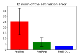
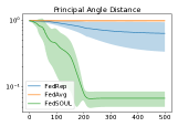
Figure 2: Small data sets - synthetic data.

Figure 2 compares the different approaches by computing the principle angle distance (respectively the $\ell_{2}$ norm) between $\phi_{\mathrm{true}}$ (respectively $z^{(i)}_{\mathrm{true}}$) and its estimated value; the lesser the better. In contrast to its main competitors and based on both metrics, FedSOUL provides an impressive improvement. This illustrates the benefits of the introduction of a common prior $p(z^{(i)}\mid\beta)$ which allows to prevent from overfitting on clients with small data sets while performing personalisation. Additional results with other choices for $(b,d,k)$ and data partitioning strategies are available in the supplement.

Moreover, to compare our algorithm with a non-FL setting, we perform a non-distributed and non-federated stochastic approximation algorithm to find $\theta^{\ast}$ using a large number of iterations to get an accurate approximation of the optimal parameter $\theta^{\ast}$. Then, we use FedPop to obtain an estimate $\tilde{\theta^{\ast}}$ and measure the relative error in $l_{2}$- distance between $\theta^{\ast}$ and $\tilde{\theta^{\ast}}$. For some outer iterations $T=100$, the relative error was less than $10^{-3}$, which illustrates the relevance of our theoretical results. We also test the performances of the proposed approach when the warm-start strategy is not used. In this case, we have to set $M=50$ to achieve the same performances as in the stateful variant of FedSOUL.

Real Data. We consider now real image data sets, namely CIFAR-10 and CIFAR-100 (Krizhevsky, 2009). For our likelihood model defined by $p(\mathrm{D}_{i}\mid\phi,z^{(i)})$, we use 5-layer convolutional neural networks and perform personalisation for the last layer. We set $b=100$ for convenience and control data heterogeneity by assigning to each client $N_{i}$ images belonging to only $S$ different classes.

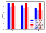
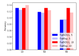
Figure 3: (right) CIFAR-10 with $S=5$ and (left) CIFAR-100 with $S=20$. The $x$-axis refers to the percentage of clients having $N_{i}\in\{5,10\}$ images.

Small data sets. Under this setting, we first consider (10%, 50%, 90%) of clients having small data sets of size either $N_{i}=5$ or $N_{i}=10$; while remaining clients have larger data sets of size $N_{i}=25$. We compare our approach with FedRep since it stands for the state-of-the-art personalised FL approach. The algorithms are trained fulfilling the same computational budget. Figure 3 shows the average accuracy across clients for the two approaches on both CIFAR-10 and CIFAR-100. We can see that FedSOUL is consistently better than FedRep over different configurations.

Full data sets. In addition to show that the proposed approach achieves state-of-the-art performances on small data sets (which is common in the cross-device scenario), we now illustrate that FedSOUL is also competitive on larger data sets. To this end, we use all training images in CIFAR-10 and CIFAR-100 image data sets and consider the same data partitioning as in Collins et al. (2021). More precisely, in this case the number of observations and the number of classes per client are uniformly shared over the clients. Table 2 shows our results in comparison with state-of-the-art personalised FL approaches. We can see that that our model outperforms other methods on both CIFAR-10 and CIFAR-100 by a large margin. Additional results with other personalised FL algorithms are postponed to the supplement.

Uncertainty Quantification on Real Data. As highlighted in Table 1, one advantage of the proposed approach compared to existing personalised FL methods is the ability to perform uncertainty quantification by sampling locally from the posterior $p(z^{(i)}\mid\mathrm{D}_{i},\phi_{K},\beta_{K})$, see Algorithm 1. We illustrate this feature by computing on CIFAR-10 calibration curves and scores (e.g. expected calibration error aka ECE) on a specific client; and by performing an out-of-distribution analysis on MNIST/FashionMNIST data sets. Figure 4 shows that the proposed approach provides relevant uncertainty diagnosis. Additional results on uncertainty quantification can be found in the supplement.

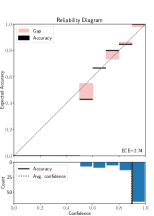
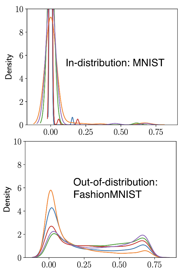
Figure 4: (right) Calibration on CIFAR-10 for a specific client and (left) OOD analysis with MNIST training & FashionMNIST inference – one curve corresponds to one client.

Table 2: Real data - Full data sets. Accuracy (in %) on test samples. FedAvg and SCAFFOLD are not personalised FL approaches but stand for well-known FL benchmarks.

	CIFAR-10		CIFAR-100
(# clients $b$, # classes per client $S$)	(100, 2)	(100, 5)	(100, 5)	(100, 20)
Local learning only	89.79	70.68	75.29	41.29
FedAvg (McMahan et al., 2017)	42.65	51.78	23.94	31.97
SCAFFOLD (Karimireddy et al., 2020)	37.72	47.33	20.32	22.52
LG-FedAvg (Liang et al., 2019)	84.14	63.02	72.44	38.76
Per-FedAvg (Fallah et al., 2020)	82.27	67.20	72.05	52.49
L2GD (Hanzely and Richtárik, 2020)	81.04	59.98	72.13	42.84
APFL (Deng et al., 2021b)	83.77	72.29	78.20	55.44
DITTO (Li et al., 2021)	85.39	70.34	78.91	56.34
FedRep (Collins et al., 2021)	87.70	75.68	79.15	56.10
FedAvg + fine-tuning (FT)	85.63	71.32	79.03	56.19
FedSOUL (this paper)	91.12	79.48	79.56	59.73

6 Conclusion

In this paper, we proposed a general Bayesian methodology based on a natural mixed-effects modeling approach to model personalisation in federated learning. Our FL method is the first that allows for both personalisation and cheap uncertainty quantification for (cross-device) federated learning. By introducing a common prior on the local parameters, we tackle the local overfitting problem in the scenario where clients have highly heterogeneous and small data sets. In addition, we have shown that the proposed approach has favorable convergence properties. Some limitations of FedPop pave the way for more advanced personalised FL approaches. As an example, our model does not allow for training heterogeneous architectures across clients because of the introduced common prior, and only satisfy first-order privacy guarantees. Regarding the latter, further works include for instance deriving differentially private versions of our framework.

Checklist

The checklist follows the references. Please read the checklist guidelines carefully for information on how to answer these questions. For each question, change the default [TODO] to [Yes] , [No] , or [N/A] . You are strongly encouraged to include a justification to your answer, either by referencing the appropriate section of your paper or providing a brief inline description. For example:

• Did you include the license to the code and datasets? [Yes] See Section LABEL:gen_inst.

• Did you include the license to the code and datasets? [No] The code and the data are proprietary.

• Did you include the license to the code and datasets? [N/A]

Please do not modify the questions and only use the provided macros for your answers. Note that the Checklist section does not count towards the page limit. In your paper, please delete this instructions block and only keep the Checklist section heading above along with the questions/answers below.

1. For all authors…

   1. Do the main claims made in the abstract and introduction accurately reflect the paper’s contributions and scope? [Yes]

   2. Did you describe the limitations of your work? [Yes] We describe these limitations in the conclusion.

   3. Did you discuss any potential negative societal impacts of your work? [N/A]

   4. Have you read the ethics review guidelines and ensured that your paper conforms to them? [Yes]

2. If you are including theoretical results…

   1. Did you state the full set of assumptions of all theoretical results? [Yes] Some assumptions are explicitly stated in Section 3. For the sake of readability and due to the space limit, we postponed other technical assumptions in the supplement.

   2. Did you include complete proofs of all theoretical results? [Yes] All our proofs are postponed to the supplement.

3. If you ran experiments…

   1. Did you include the code, data, and instructions needed to reproduce the main experimental results (either in the supplemental material or as a URL)? [Yes] See the supplement.

   2. Did you specify all the training details (e.g., data splits, hyperparameters, how they were chosen)? [Yes] Some details have been stated in Section 5 in the main paper. Because of the limited number of pages, others have been postponed to the supplement.

   3. Did you report error bars (e.g., with respect to the random seed after running experiments multiple times)? [Yes] We did it for some experiments we conducted, see e.g. Figure 2.

   4. Did you include the total amount of compute and the type of resources used (e.g., type of GPUs, internal cluster, or cloud provider)? [Yes] This is postponed to the supplement.

4. If you are using existing assets (e.g., code, data, models) or curating/releasing new assets…

   1. If your work uses existing assets, did you cite the creators? [Yes] See for example the citation for CIFAR image data sets.

   2. Did you mention the license of the assets? [N/A]

   3. Did you include any new assets either in the supplemental material or as a URL? [N/A]

   4. Did you discuss whether and how consent was obtained from people whose data you’re using/curating? [N/A]

   5. Did you discuss whether the data you are using/curating contains personally identifiable information or offensive content? [N/A]

5. If you used crowdsourcing or conducted research with human subjects…

   1. Did you include the full text of instructions given to participants and screenshots, if applicable? [N/A]

   2. Did you describe any potential participant risks, with links to Institutional Review Board (IRB) approvals, if applicable? [N/A]

   3. Did you include the estimated hourly wage paid to participants and the total amount spent on participant compensation? [N/A]

SUPPLEMENTARY MATERIAL

Notations and conventions.

For the sake of simplicity, with little abuse, we shall use the same notations for a probability distribution and its associated probability density function. For $n\geq 1$, we refer to the set of integers between $1$ and $n$ with the notation $[n]$. The $d$-multidimensional Gaussian probability distribution with mean $\mu\in\mathbb{R}^{d}$ and covariance matrix $\Sigma\in\mathbb{R}^{d\times d}$ is denoted by $\mathrm{N}(\mu,\Sigma)$. Equations of the form (1) (resp. (S1)) refer to equations in the main paper (resp. in the supplement).

Denote by $\mathcal{B}(\mathbb{R}^{d})$ the Borel $\sigma$-field of $\mathbb{R}^{d}$, and for $f:\mathbb{R}^{d}\to\mathbb{R}$ measurable, $\left\|{f}\right\|_{\infty}=\sup_{x\in\mathbb{R}^{d}}\left\lvert{f(x)}\right\rvert$. For $\mu$ a probability measure on $(\mathbb{R}^{d},\mathcal{B}(\mathbb{R}^{d}))$ and $f$ a $\mu$-integrable function, denote by $\mu(f)$ the integral of $f$ w.r.t. $\mu$. For $f:\ \mathbb{R}^{d}\to\mathbb{R}$ measurable, the $V$-norm of $f$ is given by $\|f\|_{V}=\sup_{x\in\mathbb{R}^{d}}|f(x)|/V(x)$. Let $\xi$ be a finite signed measure on $(\mathbb{R}^{d},\mathcal{B}(\mathbb{R}^{d}))$. The $V$-total variation distance of $\xi$ is defined as

$$\textstyle{\|\xi\|_{V}=\sup_{\|f\|_{V}\leq 1}\left\lvert{\int_{\mathbb{R}^{d}}f(x)\mathrm{d}\xi(x)}\right\rvert\,.}$$ (S1)

If $V=1$, then $\|\cdot\|_{V}$ is the total variation denoted by $\|\cdot\|_{\mathrm{TV}}$. Let $\mathsf{U}$ be an open set of $\mathbb{R}^{d}$. We denote by $\mathrm{C}^{k}(\mathsf{U},\mathbb{R}^{p})$ the set of $\mathbb{R}^{p}$-valued $k$-differentiable functions, respectively the set of compactly supported $\mathbb{R}^{p}$-valued and $k$-differentiable functions. Let $f:\mathsf{U}\to\mathbb{R}$, we denote by $\nabla f$, the gradient of $f$ if it exists. $f$ is said to me $\mathtt{m}$-convex with $m\geq 0$ if for all $x,y\in\mathbb{R}^{d}$ and $t\in\left[0,1\right]$,

$$f(tx+(1-t)y)\leq tf(x)+(1-t)f(y)-\mathtt{m}t(1-t)\left\|{x-y}\right\|^{2}/2\,.$$ (S2)

For any $a\in\mathbb{R}^{d}$ and $R>0$, denote $\operatorname{B}(a,R)$ the open ball centered at $a$ with radius $R$. Let $(\mathsf{X},\mathcal{X})$ and $(\mathsf{Y},\mathcal{Y})$ be two measurable spaces. A Markov kernel $\mathrm{P}$ is a mapping $\mathrm{K}:\ \mathsf{X}\times\mathcal{Y}\to\left[0,1\right]$ such that for any $x\in\mathsf{X}$, $\mathrm{P}(x,\cdot)$ is a probability measure and for any $\mathsf{A}\in\mathcal{Y}$, $\mathrm{P}(\cdot,\mathsf{A})$ is measurable. For any probability measure $\mu$ on $(\mathsf{X},\mathcal{X})$ and measurable function $f:\mathsf{Y}\to\mathbb{R}_{+}$ we denote $\mu\mathrm{P}=\int_{\mathsf{X}}\mathrm{P}(x,\cdot)\mathrm{d}\mu(x)$ and $\mathrm{P}f=\int_{\mathsf{Y}}f(y)\mathrm{P}(\cdot,\mathrm{d}y)$. In what follows the Dirac mass at $x\in\mathbb{R}^{d}$ by $\updelta_{x}$.

Contents

1. 1 Introduction
2. 2 Proposed Approach
3. 3 Theoretical Guarantees
4. 4 Related Works
5. 5 Numerical Experiments
6. 6 Conclusion
7. S1 Theoretical analysis of FedSOUK
   1. S1.1 Preliminaries
   2. S1.2 Main Assumptions
   3. S1.3 Stochastic Approximation Framework
   4. S1.4 Main Result
   5. S1.5 Supporting Lemmata
8. S2 Application to FedSOUL
   1. S2.1 Assumptions
   2. S2.2 Verification of 6 and 7
9. S3 Additional Experiments
   1. S3.1 Synthetic datasets
   2. S3.2 Image datasets classification
   3. S3.3 Image datasets uncertainty quantification

Appendix S1 Theoretical analysis of FedSOUK

This section aims at recasting the proposed methodology into a stochastic approximation framework and at stating the main assumptions required to show our theoretical results regarding FedSOUK, which uses a general unadjusted Markov kernel. Then, we will use these general results to show non-asymptotic convergence guarantees for FedSOUL, which considers an unadjusted Markov kernel associated to overdamped Langevin dynamics.

S1.1 Preliminaries

We first show that FedSOUK (see Algorithm 1 in the main paper) can be cast into a general stochastic approximation (SA) framework which corresponds to a federated variant of the stochastic optimization via unadjusted kernel (SOUK) approach proposed in De Bortoli et al. (2021). Then, the convergence guarantees for FedSOUK will follow by generalizing the proof techniques used to analyze SOUK.

Recall that $\theta=(\phi,\beta)\in\Theta$ corresponds to the parameter we are seeking to optimize where $\Theta=\Phi\times\mathsf{B}\subset\mathbb{R}^{d_{\Theta}}$. Define $f:\Theta\to\mathbb{R}$ of the form

$$f(\theta)=b^{-1}\sum_{i=1}^{b}f_{i}(\theta)\,,$$ (S3)

where for any $i\in[b]$ and $\theta\in\Theta$,

$$f_{i}\left({\theta}\right)=-\log p(\theta)-b\log p\left({\mathrm{D}_{i}\mid\phi,\beta}\right)\,,$$ (S4)

where $p(\theta)=p(\phi,\beta)=p(\phi)p(\beta)$ and for any $i\in[b]$, $p(\mathrm{D}_{i}\mid\phi,\beta)$ is defined in (1). Then, under these notations, (4) can be written as

$$\theta^{\star}=\operatornamewithlimits{\arg\min}_{\theta\in\Theta}f(\theta)\,.$$ (S5)

In addition, based on (10) and (11), the gradient of $f_{i}$ defined in (S4) admits the form for $i\in[b]$,

$$\nabla f_{i}:\begin{cases}\mathbb{R}^{d_{\Phi}+d_{\mathsf{B}}}\to\mathbb{R}^{d_{\Theta}}\\ \theta\mapsto\int_{\mathbb{R}^{d}}H^{(i)}_{\theta}\left({z^{(i)}}\right)\pi_{\theta}^{(i)}\left({\mathrm{d}z^{(i)}}\right)\,,\end{cases}$$ (S6)

where, for any $i\in[b]$ and $\theta\in\Theta$, $\pi_{\theta}^{(i)}:z^{(i)}\mapsto p(z^{(i)}\mid\mathrm{D}_{i},\theta)$ and for any $\theta\in\Theta$, $H_{\theta}^{(i)}:z^{(i)}\mapsto-\nabla_{\theta}\log p(\theta)-b\nabla_{\theta}\log p(\mathrm{D}_{i},z^{(i)}\mid\theta)$.

S1.2 Main Assumptions

We make the following assumption on $\Theta$ and the family of functions $\{f_{i}:i\in[b]\}$.

A 1.

$\Theta$ is a convex, closed subset of $\mathbb{R}^{d_{\Theta}}$ and $\Theta\subset\mathrm{B}(0,R_{\Theta})$ for $R_{\Theta}>0$.

A 2.

For any $i\in[b]$, the following conditions hold.

1. The function $f_{i}$ defined in (S3) is convex.

2. There exist an open set $\mathsf{U}\in\mathbb{R}^{d_{\Theta}}$ and $L_{f}>0$ such that $\Theta\subset\mathsf{U}$, $f_{i}\in\mathrm{C}^{1}(\mathsf{U},\mathbb{R})$ and for any $\theta_{1},\theta_{2}\in\Theta$,

   $$\left\|{\nabla f_{i}(\theta_{2})-\nabla f_{i}(\theta_{1})}\right\|\leq L_{f}\left\|{\theta_{2}-\theta_{1}}\right\|\,.$$

Note that 2-(ii) implies that the objective function $f$ defined in (S3) is gradient-Lipschitz with Lipschitz constant $L_{f}$.

We now consider assumptions on the family of compression and partial participation operators $\{\mathscr{C}_{i},\mathscr{S}_{i}\}_{i\in[b]}$.

A 3.

There exists a probability measure $\nu_{1}$ on a measurable space $(\mathsf{X}_{1},\mathcal{X}_{1})$ and a family of measurable functions $\{\mathscr{C}_{i}:\mathbb{R}^{d_{\Phi}}\times\mathsf{X}_{1}\to\mathbb{R}^{d_{\Phi}}\}_{i\in[b]}$ such that the following conditions hold.

1. For any $v\in\mathbb{R}^{d_{\Phi}}$ and any $i\in[b]$, $\int_{\mathsf{X}_{1}}\mathscr{C}_{i}(v,x^{(1)})\,\nu_{1}(\mathrm{d}x^{(1)})=v$.

2. There exist $\{\omega_{i}\in\mathbb{R}_{+}\}_{i\in[b]}$, such that for any $v\in\mathbb{R}^{d_{\Phi}}$ and any $i\in[b]$,

   $$\int_{\mathsf{X}_{1}}\left\|{\mathscr{C}_{i}(v,x^{(1)})-v}\right\|^{2}\,\nu_{1}(\mathrm{d}x^{(1)})\leq\omega_{i}\left\|{v}\right\|^{2}\,.$$ (S7)

In addition, recall that we consider the partial device participation context where at each communication round $k\geq 1$, each client has a probability $p_{i}\in(0,1]$ of participating, independently from other clients.

A 4.

For any $i\in[b]$, the unbiased partial participation operator $\mathscr{S}_{i}:\mathbb{R}^{d_{\Theta}}\times\mathsf{X}_{2}\to\mathbb{R}^{d_{\Theta}}$ is defined, for any $\theta\in\mathbb{R}^{d_{\Theta}}$ and $x^{(2)}=\{x^{(2)}_{i}\}_{i\in[b]}\in\mathsf{X}_{2}$ with $\mathsf{X}_{2}=[0,1]^{b}$ by

$$\mathscr{S}_{i}(\theta,x^{(2)})=\mathbf{1}\{x^{(2)}_{i}\leq p_{i}\}\theta/p_{i}\,,$$ (S8)

where $p_{i}\in(0,1]$.

Note that the assumption 4 is equivalent to 4 in the main paper.

Let $V:\mathbb{R}^{d}\rightarrow[1,\infty)$ a measurable function. We consider the following assumption on the family $\{(H_{\theta}^{(i)},\pi_{\theta}^{(i)})\,:\,\theta\in\Theta,i\in[b]\}$.

A 5.

For any $i\in[b]$, the following conditions hold.

1. For any $\theta\in\Theta$, $\pi_{\theta}^{(i)}(\|H_{\theta}^{(i)}\|)<\infty$ and $(\theta,z^{(i)})\mapsto H_{\theta}^{(i)}(z^{(i)})$ is measurable.

2. There exists $L_{H}\geq 0$ such that for any $z\in\mathbb{R}^{d}$ and $\theta_{1},\theta_{2}\in\Theta$,

   $$\left\|{H_{\theta_{2}}^{(i)}(z)-H_{\theta_{1}}^{(i)}(z)}\right\|\leq L_{H}\left\|{\theta_{2}-\theta_{1}}\right\|V^{1/2}(z)\,.$$

S1.3 Stochastic Approximation Framework

Let $(X_{k}^{(i,1)})_{k\in\mathbb{N},i\in[b]}$ a sequence of independent an identically distributed (i.i.d.) random variables with distribution $\nu_{1}$ independent of the sequence $(X_{k}^{(i,2)})_{k\in\mathbb{N},i\in[b]}$ which is i.i.d. and with uniform distribution on $[0,1]$. We consider a family of unadjusted Markov kernels $\{Q^{(i)}_{\gamma,\theta}:\gamma\in(0,\bar{\gamma}],\theta\in\Theta,i\in[b]\}$. Let $(\gamma_{k})_{k\in\mathbb{N}^{*}}\in(\mathbb{R}^{*}_{+})^{\mathbb{N}^{*}}$ a sequence of step-sizes which will be used to obtain approximate samples from $\pi_{\theta}^{(i)}$ using $Q^{(i)}_{\gamma,\theta}$.

We now recast the proposed approach detailed in Algorithm 1 into a stochastic approximation framework.

Starting from some initialization $(Z_{0}^{(1,0)},\ldots,Z_{0}^{(b,0)},\theta_{0})\in\mathbb{R}^{bd}\times\Theta$, we define on a probability space $(\Omega,\mathcal{F},\mathbb{P})$, the sequence $((Z_{k}^{(1,m)},\ldots,Z_{k}^{(b,m)})_{m\in[M]},\theta_{k})_{k\in\mathbb{N}}$ via the recursion for $k\in\mathbb{N}$,

$$\text{ for any $i\in[b]$, given $\mathcal{F}_{k-1}$},(Z_{k}^{(i,m)})_{m\in\{0,\ldots,M\}}\text{ is a Markov chain with Markov kernel $Q^{(i)}_{\gamma_{k},\theta_{k}}$}$$ (S9)

with $$Z_{k}^{(i,0)}=Z_{k-1}^{(i,M)}$$  , (S10)

$$\theta_{k+1}=\Pi_{\Theta}\left[{\theta_{k}-\bm{\eta}_{k+1}\odot\bm{\Delta}_{\theta_{k}}\left({Z_{k+1}^{(1:M)},X_{k+1}^{(1)},X_{k+1}^{(2)}}\right)}\right]\,,$$ (S11)

where $\odot$ denotes the Hadamard product and for any $k\in\mathbb{N}$, $\mathcal{F}_{k}=\sigma(\theta_{0},\{\{Z^{(i,m)}_{l}\}_{m\in[M]}\,:\,l\in\{0,\ldots,k\}\,,\,i\in[b]\})$ and $\mathcal{F}_{-1}=\sigma(\theta_{0},\{Z_{0}^{(i,0)}\,:\,i\in[b]\})$. In addition, for any $k\in\mathbb{N}$, $\bm{\eta}_{k+1}=(\eta_{k+1}^{(1)},\eta_{k+1}^{(2)})^{\top}$, $Z_{k+1}^{(1:M)}=([Z_{k+1}^{(1,1:M)}]^{\top},\ldots,[Z_{k}^{(b,1:M)}]^{\top})^{\top}$ and for any $\theta\in\Theta$, $z^{(1:M)}\in\mathbb{R}^{Md}$, $x^{(1)}\in\mathsf{X}_{1}$, $x^{(2)}\in\mathsf{X}_{2}$ ,

$$\bm{\Delta}_{\theta}\left({z^{(1:M)},x^{(1)},x^{(2)}}\right) =\begin{pmatrix}\Delta_{\phi}\left({z^{(1:M)},x^{(1)},x^{(2)}}\right)\\ \Delta_{\beta}\left({z^{(1:M)},x^{(2)}}\right)\end{pmatrix}\,,$$ (S12)

$$=\begin{pmatrix}\sum_{i=1}^{b}\mathscr{S}_{i}\left[{\mathscr{C}_{i}\left({\Delta_{\phi}^{(i)}(z^{(i,1:M)}),x^{(i,1)}}\right),x^{(i,2)}}\right]\\ \sum_{i=1}^{b}\mathscr{S}_{i}\left[{\Delta_{\beta}^{(i)}(z^{(i,1:M)}),x^{(i,2)}}\right]\end{pmatrix}\,,$$ (S13)

where $\{\Delta_{\beta}^{(i)},\Delta_{\phi}^{(i)}\}_{i\in[b]}$ defined by

$$\Delta_{\beta}^{(i)}(z^{(i,1:M)}) =-\frac{1}{M}\sum_{m=1}^{M}\left\{{(1/b)\nabla_{\beta}p(\beta)+\nabla_{\beta}\log p({\textstyle{z^{(i,m)}\mid\beta}})}\right\}$$ (S14)

$$\Delta_{\phi}^{(i)}(z^{(i,1:M)}) =-\frac{1}{M}\sum_{m=1}^{M}\left\{{(1/b)\nabla_{\phi}p(\phi)+\nabla_{\phi}\log p({\textstyle{\mathrm{D}_{i}\mid z^{(i,m)},\phi}})}\right\}\,.$$ (S15)

S1.4 Main Result

In order to show non-asymptotic convergence guarantees for FedSOUK detailed in Algorithm 1, we need additional assumptions ensuring some stability of the sequence $(Z_{k}^{(i,m)}\,:\,m\in\{0,\ldots,M\},i\in[b])_{k\in\mathbb{N}}$. These conditions are stated hereafter.

A 6.

For any $i\in[b]$, the following conditions hold.

1. There exists $A_{1}\geq 1$ such that for any $p,k\in\mathbb{N}$ and $m\in\{0,\ldots,M\}$,

   $$\mathbb{E}\left[{[Q^{(i)}_{\gamma_{k},\theta_{k}}]^{p}V(Z^{(i,m)}_{k})\mid Z^{(i,0)}_{0}}\right]\leq A_{1}V(Z^{(i,0)}_{0})\,,\ \mathbb{E}\left[{V(Z^{(i,0)}_{0})}\right]<\infty\,,$$

   where $(Z_{k}^{(i,m)}\,:\,m\in\{0,\ldots,M\},i\in[b])_{k\in\mathbb{N}}$ is defined in (S10).

2. There exists $A_{2},A_{3}\geq 1$, $\rho\in[0,1)$ such that for any $\gamma\in(0,\bar{\gamma}]$, $\theta\in\Theta$, $z\in\mathbb{R}^{d}$ and $k\in\mathbb{N}$, $Q^{(i)}_{\gamma,\theta}$ admits $\pi_{\gamma,\theta}^{(i)}$ as stationary distribution and

   $$\left\|{\updelta_{z}[Q^{(i)}_{\gamma,\theta}]^{k}-\pi_{\gamma,\theta}^{(i)}}\right\|_{V} \leq A_{2}\rho^{k\gamma}V(z)$$ (S16)

   $$\pi_{\gamma,\theta}^{(i)}(V) \leq A_{3}\,.$$ (S17)

3. There exists $\bm{\Psi}:\mathbb{R}_{+}^{*}\rightarrow\mathbb{R}_{+}$ such that for any $\gamma\in(0,\bar{\gamma}]$ and $\theta\in\Theta$,

   $$\left\|{\pi_{\gamma,\theta}^{(i)}-\pi_{\theta}^{(i)}}\right\|_{V^{1/2}}\leq\bm{\Psi}(\gamma)\,.$$ (S18)

A 7.

There exists a measurable function $V:\mathbb{R}^{d}\rightarrow[1,\infty)$, $\bm{\Gamma}_{1}:(\mathbb{R}^{*}_{+})^{2}\rightarrow\mathbb{R}_{+}$ and $\bm{\Gamma}_{2}:(\mathbb{R}^{*}_{+})^{2}\rightarrow\mathbb{R}_{+}$ such that for any $\gamma_{1},\gamma_{2}\in(0,\bar{\gamma}]$ with $\gamma_{2}<\gamma_{1}$, $\theta_{1},\theta_{2}\in\Theta$, $z\in\mathbb{R}^{d}$, $a\in[1/4,1/2]$, we have for any $i\in[b]$,

$$\left\|{\updelta_{z}Q_{\gamma_{2},\theta_{2}}^{(i)}-\updelta_{z}Q_{\gamma_{1},\theta_{1}}^{(i)}}\right\|_{V^{a}}\leq[\bm{\Gamma}_{1}(\gamma_{1},\gamma_{2})+\bm{\Gamma}_{2}(\gamma_{1},\gamma_{2})\left\|{\theta_{2}-\theta_{1}}\right\|]V^{2a}(z)\,.$$

We are now ready to show our main result. To ease the presentation, assume for any $k\in\mathbb{N}$ that $\eta^{(1)}_{k+1}=\eta^{(2)}_{k+1}=\eta_{k+1}$ and, for any $i\in[b],\gamma_{k+1}^{(i)}=\gamma_{k+1}$.

Theorem S2.

Assume 1, 2, 3, 4, 5, 6 and 7 and let for any $k\in[K]$, $\eta_{k}\in(0,1/L_{f}]$. In addition, for any $\theta\in\Theta$, $z\in\mathbb{R}^{d}$ and $i\in[b]$, assume that $\|H^{(i)}_{\theta}(z)\|\leq V^{1/4}(z)$. Then, for any $K\in\mathbb{N}^{*}$, we have

$$\mathbb{E}\left[{\frac{\sum_{k=1}^{K}\eta_{k}\{f(\theta_{k})-f(\theta^{\star})\}}{\sum_{k=1}^{K}\eta_{k}}}\right] \leq\frac{E_{K}}{\sum_{k=1}^{K}\eta_{k}}\,,$$ (S19)

where, for any $K\in\mathbb{N}^{*}$,

$$E_{K} =2R_{\Theta}^{2}+2A_{1}\sup_{i\in[b],m\in[M]}\left\{{\mathbb{E}\left[{V^{1/2}(Z_{0}^{(i,m)})}\right]}\right\}\sum_{k=1}^{K}\eta_{k}^{2}\left({8bL_{f}^{2}R_{\Theta}^{2}+\sum_{i=1}^{b}\frac{(\omega_{i}+1+p_{i})}{p_{i}}}\right)$$ (S20)

$$+b\sup_{i\in[b],m\in[M]}\left\{{C_{3}^{(i,m)}}\right\}\left[{\sum_{k=1}^{K}|\eta_{k}-\eta_{k-1}|\gamma_{k-1}^{-1}+\sum_{k=1}^{K}\eta_{k}^{2}\gamma_{k-1}^{-1}+\eta_{K}/\gamma_{K}-\eta_{1}/\gamma_{1}}\right]$$ (S21)

$$+b.A_{1}C_{c,2}\sup_{i\in[b],m\in[M]}\left\{{\mathbb{E}\left[{V(Z_{0}^{(i,m)})}\right]}\right\}\sum_{k=1}^{K}\eta_{k}\gamma_{k}^{-1}\left[{\gamma_{k}^{-1}\left\{{\bm{\Lambda}_{1}(\gamma_{k-1},\gamma_{k})+\bm{\Lambda}_{2}(\gamma_{k-1},\gamma_{k})\eta_{k}}\right\}+\eta_{k}}\right]$$ (S22)

$$+b\sum_{k=1}^{K}\eta_{k}\bm{\Psi}(\gamma_{k-1})\,,$$ (S23)

with $\{C_{3}^{(i,m)}\}_{i\in[b],m\in[M]}$ defined in Lemma S5 and $C_{c,2}$ defined in Lemma S6.

Proof.

The proof follows by using the fact that (S96) is a $(\mathcal{F}_{k-1})_{k\in\mathbb{N}^{*}}$-martingale increment and by combining Lemma S1-S7. ∎

S1.5 Supporting Lemmata

For convenience, we define the following quantities that will naturally appear in our derivations. For any $k\in\mathbb{N}^{*}$, let

$$\bm{\epsilon}_{k}=\bm{\Delta}_{\theta_{k-1}}\left({Z_{k}^{(1:M)},X_{k}^{(1)},X_{k}^{(2)}}\right)-\nabla f(\theta_{k-1})\,,$$ (S24)

where $\bm{\Delta}_{\theta}$ is defined in (S13).

The following lemma first provides a non-asymptotic upper bound on $\sum_{k=1}^{K}\eta_{k}\{f(\theta_{k})-f(\theta^{\star})\}$ involving key quantities to control such as the Monte Carlo approximation error term (S24).

Lemma S1.

Assume 1 and 2, and let for any $k\in[K]$, $\eta_{k}\in(0,1/L_{f}]$. Then, for any $K\in\mathbb{N}^{*}$, we have

$$\sum_{k=1}^{K}\eta_{k}\{f(\theta_{k})-f(\theta^{\star})\} \leq 2R_{\Theta}^{2}+\sum_{k=1}^{K}\eta_{k}^{2}\left\|{\bm{\epsilon}_{k}}\right\|^{2}-\sum_{k=1}^{K}\eta_{k}\left\langle\Pi_{\Theta}\left({\theta_{k-1}-\eta_{k}\nabla f(\theta_{k-1})}\right)-\theta^{\star},\bm{\epsilon}_{k}\right\rangle\,,$$ (S25)

where $\{\bm{\epsilon}_{k}\}_{k=1}^{K}$ is defined in (S24).

Proof.

Let $k\in\mathbb{N}$. Since $\Theta$ is closed and convex by 1, the indicator function $\iota_{\Theta}$, defined for any $u\in\mathbb{R}^{d_{\Phi}+d_{\mathsf{B}}}$ by $\iota_{\Theta}(u)=0$ if $u\in\Theta$ and $\iota_{\Theta}(u)=\infty$ otherwise, is lower semi-continuous and convex. Therefore by Atchadé et al. (2017, Lemma 7) we have

$$\iota_{\mathsf{B}}(\beta_{k+1})-\iota_{\mathsf{B}}(\beta_{\star}) \leq-\frac{1}{\eta_{k+1}}\left\langle\beta_{k+1}-\beta_{\star},\beta_{k+1}-\beta_{k}+\eta_{k+1}\Delta_{\beta_{k}}\left({Z_{k+1}^{(1:M)},X_{k+1}^{(2)}}\right)\right\rangle\,,$$ (S26)

$$\iota_{\Phi}(\phi_{k+1})-\iota_{\Phi}(\phi_{\star}) \leq-\frac{1}{\eta_{k+1}}\left\langle\phi_{k+1}-\phi_{\star},\phi_{k+1}-\phi_{k}+\eta_{k+1}\Delta_{\phi_{k}}\left({Z_{k+1}^{(1:M)},X_{k+1}^{(1)},X_{k+1}^{(2)}}\right)\right\rangle\,,$$ (S27)

where $\theta^{\star}=(\phi_{\star},\beta_{\star})$ is defined in (S5). In addition by 2-(ii), we have for any $i\in[b]$,

$$f_{i}(\theta_{k+1})-f_{i}(\theta_{k})\leq\langle\nabla f_{i}(\theta_{k}),\theta_{k+1}-\theta_{k}\rangle+\frac{L_{f}}{2}\left\|{\theta_{k+1}-\theta_{k}}\right\|^{2}\,.$$ (S28)

Using (S28) and the fact that for any $k\in\mathbb{N}$, $\eta_{k+1}\leq 1/L_{f}$, we have

$$f(\theta_{k+1})-f(\theta_{k}) \leq\langle\nabla_{\beta}f(\theta_{k}),\beta_{k+1}-\beta_{k}\rangle+\frac{L_{f}}{2}\left\|{\beta_{k+1}-\beta_{k}}\right\|^{2}$$ (S29)

$$+\langle\nabla_{\phi}f(\theta_{k}),\phi_{k+1}-\phi_{k}\rangle+\frac{L_{f}}{2}\left\|{\phi_{k+1}-\phi_{k}}\right\|^{2}$$ (S30)

$$\leq\langle\nabla_{\beta}f(\theta_{k}),\beta_{k+1}-\beta_{k}\rangle+\frac{1}{2\eta_{k+1}}\left\|{\beta_{k+1}-\beta_{k}}\right\|^{2}$$ (S31)

$$+\langle\nabla_{\phi}f(\theta_{k}),\phi_{k+1}-\phi_{k}\rangle+\frac{1}{2\eta_{k+1}}\left\|{\phi_{k+1}-\phi_{k}}\right\|^{2}\,.$$ (S32)

Finally, 2-(i) implies for any $i\in[b]$,

$$f_{i}(\theta_{k})-f_{i}(\theta^{\star})\leq-\langle\nabla f_{i}(\theta_{k}),\theta_{\star}-\theta_{k}\rangle\,.$$ (S33)

For any $i\in[b]$, let $F_{i}=f_{i}+\iota_{\Theta}$ and let $F=(1/b)\sum_{i=1}^{b}F_{i}$. Using this notation and combining (S26), (S27), (S32) and (S33), we have

$$F(\theta_{k+1})-F(\theta^{\star})$$ (S34)

$$= \ f(\theta_{k+1})-f(\theta_{k})+f(\theta_{k})-f(\theta^{\star})+\iota_{\Phi}(\phi_{k+1})-\iota_{\Phi}(\phi_{\star})+\iota_{\mathsf{B}}(\beta_{k+1})-\iota_{\mathsf{B}}(\beta_{\star})$$ (S35)

$$\leq -\left\langle\beta_{k+1}-\beta_{\star},\Delta_{\beta_{k}}\left({Z_{k+1}^{(i,1:M)},X_{k+1}^{(2)}}\right)-\nabla_{\beta}f(\theta_{k})\right\rangle-\left\langle\beta_{k+1}-\beta_{\star},\beta_{k+1}-\beta_{k}\right\rangle$$ (S36)

$$-\left\langle\phi_{k+1}-\phi_{\star},\Delta_{\phi_{k}}\left({Z_{k+1}^{(1:M)},X_{k+1}^{(1)},X_{k+1}^{(2)}}\right)-\nabla_{\phi}f(\theta_{k})\right\rangle-\left\langle\phi_{k+1}-\phi_{\star},\phi_{k+1}-\phi_{k}\right\rangle$$ (S37)

$$+\frac{1}{2\eta_{k+1}}\left\|{\beta_{k+1}-\beta_{k}}\right\|^{2}+\frac{1}{2\eta_{k+1}}\left\|{\phi_{k+1}-\phi_{k}}\right\|^{2}$$ (S38)

$$= -\left\langle\theta_{k+1}-\theta_{\star},\bm{\Delta}_{\theta_{k}}\left({Z_{k+1}^{(1:M)},X_{k+1}^{(1)},X_{k+1}^{(2)}}\right)-\nabla f(\theta_{k})\right\rangle$$ (S39)

$$+\frac{1}{2\eta_{k+1}}\left[{\left\|{\phi_{k}-\phi_{\star}}\right\|^{2}-\left\|{\phi_{k+1}-\phi_{\star}}\right\|^{2}}\right]+\frac{1}{2\eta_{k+1}}\left[{\left\|{\beta_{k}-\beta_{\star}}\right\|^{2}-\left\|{\beta_{k+1}-\beta_{\star}}\right\|^{2}}\right]\,.$$ (S40)

From (S40), it follows for any $K\in\mathbb{N}^{*}$ that

$$\sum_{k=1}^{K}\eta_{k}\{F(\theta_{k})-F(\theta^{\star})\}$$ (S41)

$$\leq-\sum_{k=1}^{K}\eta_{k}\left\langle\theta_{k}-\theta_{\star},\bm{\Delta}_{\theta_{k-1}}\left({Z_{k}^{(1:M)},X_{k}^{(1)},X_{k}^{(2)}}\right)-\nabla f(\theta_{k-1})\right\rangle$$ (S42)

$$+\frac{1}{2}\left\|{\phi_{0}-\phi_{\star}}\right\|^{2}-\frac{1}{2}\left\|{\phi_{K}-\phi_{\star}}\right\|^{2}+\frac{1}{2}\left\|{\beta_{0}-\beta_{\star}}\right\|^{2}-\frac{1}{2}\left\|{\beta_{K}-\beta_{\star}}\right\|^{2}$$ (S43)

$$\leq-\sum_{k=1}^{K}\eta_{k}\left\langle\theta_{k}-\theta_{\star},\bm{\Delta}_{\theta_{k-1}}\left({Z_{k}^{(1:M)},X_{k}^{(1)},X_{k}^{(2)}}\right)-\nabla f(\theta_{k-1})\right\rangle+\frac{1}{2}\left\|{\theta_{0}-\theta^{\star}}\right\|^{2}$$ (S44)

$$=-\sum_{k=1}^{K}\eta_{k}\left\langle\theta_{k}-\Pi_{\Theta}\left({\theta_{k-1}-\eta_{k}\nabla f(\theta_{k-1})}\right),\bm{\Delta}_{\theta_{k-1}}\left({Z_{k}^{(1:M)},X_{k}^{(1)},X_{k}^{(2)}}\right)-\nabla f(\theta_{k-1})\right\rangle$$ (S45)

$$-\sum_{k=1}^{K}\eta_{k}\left\langle\Pi_{\Theta}\left({\theta_{k-1}-\eta_{k}\nabla f(\theta_{k-1})}\right)-\theta^{\star},\bm{\Delta}_{\theta_{k-1}}\left({Z_{k}^{(1:M)},X_{k}^{(1)},X_{k}^{(2)}}\right)-\nabla f(\theta_{k-1})\right\rangle$$ (S46)

$$+\frac{1}{2}\left\|{\theta_{0}-\theta^{\star}}\right\|^{2}$$ (S47)

$$\leq\sum_{k=1}^{K}\eta_{k}^{2}\left\|{\bm{\Delta}_{\theta_{k-1}}\left({Z_{k}^{(1:M)},X_{k}^{(1)},X_{k}^{(2)}}\right)-\nabla f(\theta_{k-1})}\right\|^{2}+\frac{1}{2}\left\|{\theta_{0}-\theta^{\star}}\right\|^{2}$$ (S48)

$$-\sum_{k=1}^{K}\eta_{k}\left\langle\Pi_{\Theta}\left({\theta_{k-1}-\eta_{k}\nabla f(\theta_{k-1})}\right)-\theta^{\star},\bm{\Delta}_{\theta_{k-1}}\left({Z_{k}^{(1:M)},X_{k}^{(1)},X_{k}^{(2)}}\right)-\nabla f(\theta_{k-1})\right\rangle\,,$$ (S49)

where we used Atchadé et al. (2017, Lemma 7) and the Cauchy-Schwarz inequality in the last inequality. The proof is concluded using $f\leq F$, $f(\theta^{\star})=F(\theta^{\star})$ since $\theta^{\star}\in\Theta$, and by noting that under 1 we have $\left\|{\theta_{0}-\theta^{\star}}\right\|\leq 2R_{\Theta}$. ∎

Lemma S1 involves two key quantities to upper bound namely $\left\|{\bm{\epsilon}_{k}}\right\|$ and $\left\langle\Pi_{\Theta}\left({\theta_{k-1}-\eta_{k}\nabla f(\theta_{k-1})}\right)-\theta^{\star},\bm{\epsilon}_{k}\right\rangle$ for any $k\in\mathbb{N}^{*}$. Our next lemmata aim at controlling the expectations of these two terms. In particular, Lemma S2 and Lemma S3 show that the impacts of Monte Carlo approximation, partial participation and compression can be decoupled.

To this end, define for any $k\in\mathbb{N}^{*}$ and $i\in[b]$

$$\varepsilon_{\beta,k}^{(i)} =\frac{1}{M}\sum_{m=1}^{M}H_{\beta_{k-1}}^{(i)}\left({Z_{k}^{(i,m)}}\right)-\nabla_{\beta}f_{i}(\theta_{k-1})\,,$$ (S50)

$$\varepsilon_{\phi,k}^{(i)} =\frac{1}{M}\sum_{m=1}^{M}H^{(i)}_{\phi_{k-1}}\left({Z_{k}^{(i,m)}}\right)-\nabla_{\phi}f_{i}(\theta_{k-1})\,,$$ (S51)

$$\varepsilon_{\theta,k}^{(i)} =\left[{\varepsilon_{\beta,k}^{(i)},\varepsilon_{\phi,k}^{(i)}}\right]\,,$$ (S52)

where, for any $k\in\mathbb{N}^{*}$ and $i\in[b]$, $H^{(i)}_{\theta_{k-1}}(Z_{k}^{(i,m)})=[H^{(i)}_{\phi_{k-1}}(Z_{k}^{(i,m)}),H^{(i)}_{\beta_{k-1}}(Z_{k}^{(i,m))}]$ is defined in (S6).

Lemma S2 shows that $\left\|{\bm{\epsilon}_{k}}\right\|$ can be upper bounded by a quantity involving the norm of $\{H_{\theta}^{(i)}\}_{i\in[b]}$.

Lemma S2.

Assume 1, 2, 3 and 4. Then, for any $k\in\mathbb{N}^{*}$, we have

$$\mathbb{E}\left[{\left\|{\bm{\epsilon}_{k}}\right\|^{2}}\right]\leq\frac{1}{M}\sum_{i=1}^{b}\frac{(\omega_{i}+1+p_{i})}{p_{i}}\left\{{\sum_{m=1}^{M}\mathbb{E}\left[{\left\|{H_{\theta_{k-1}}^{(i)}(Z_{k}^{(i,m)})}\right\|^{2}}\right]}\right\}+8bL_{f}^{2}R_{\Theta}^{2}\,,$$ (S53)

where $\{\bm{\epsilon}_{k}\}_{k=1}^{K}$ is defined in (S24).

Proof.

Let $k\in\mathbb{N}^{*}$. Then by using (S13), we have

$$\mathbb{E}\left[{\left\|{\bm{\epsilon}_{k}}\right\|^{2}}\right] =\mathbb{E}\left[{\left\|{\sum_{i=1}^{b}\mathscr{S}_{i}\left[{\mathscr{C}_{i}\left({\frac{1}{M}\sum_{m=1}^{M}H_{\phi_{k-1}}^{(i)}(Z_{k}^{(i,m)}),X_{k}^{(i,1)}}\right),X_{k}^{(i,2)}}\right]-\nabla_{\phi}f(\theta_{k-1})}\right\|^{2}}\right]$$ (S54)

$$+\mathbb{E}\left[{\left\|{\sum_{i=1}^{b}\mathscr{S}_{i}\left[{\frac{1}{M}\sum_{m=1}^{M}H_{\beta_{k-1}}^{(i)}(Z_{k}^{(i,m)}),X_{k}^{(i,2)}}\right]-\nabla_{\beta}f(\theta_{k-1})}\right\|^{2}}\right]\,.$$ (S55)

Using 3 and 4, it follows that

$$\mathbb{E}\left[{\left\|{\sum_{i=1}^{b}\mathscr{S}_{i}\left[{\mathscr{C}_{i}\left({\frac{1}{M}\sum_{m=1}^{M}H_{\phi_{k-1}}^{(i)}(Z_{k}^{(i,m)}),X_{k}^{(i,1)}}\right),X_{k}^{(i,2)}}\right]-\nabla_{\phi}f(\theta_{k-1})}\right\|^{2}}\right]\\ =\mathbb{E}\Bigg{[}\Big{\|}\sum_{i=1}^{b}\Big{\{}\mathscr{S}_{i}\left[{\mathscr{C}_{i}\left({\frac{1}{M}\sum_{m=1}^{M}H_{\phi_{k-1}}^{(i)}(Z_{k}^{(i,m)}),X_{k}^{(i,1)}}\right),X_{k}^{(i,2)}}\right]\\ -\mathscr{C}_{i}\left({\frac{1}{M}\sum_{m=1}^{M}H_{\phi_{k-1}}^{(i)}(Z_{k}^{(i,m)}),X_{k}^{(i,1)}}\right)\Big{\}}\Big{\|}^{2}\Bigg{]}\\ +\mathbb{E}\left[{\left\|{\sum_{i=1}^{b}\mathscr{C}_{i}\left({\frac{1}{M}\sum_{m=1}^{M}H_{\phi_{k-1}}^{(i)}(Z_{k}^{(i,m)}),X_{k}^{(i,1)}}\right)-\nabla_{\phi}f(\theta_{k-1})}\right\|^{2}}\right]\,.$$ (S56)

In addition, by 3-(i) and 3-(ii), we obtain

$$\mathbb{E}\Bigg{[}\Big{\|}\sum_{i=1}^{b}\Big{\{}\mathscr{S}_{i}\left[{\mathscr{C}_{i}\left({\frac{1}{M}\sum_{m=1}^{M}H_{\phi_{k-1}}^{(i)}(Z_{k}^{(i,m)}),X_{k}^{(i,1)}}\right),X_{k}^{(i,2)}}\right]$$ (S57)

$$-\mathscr{C}_{i}\left({\frac{1}{M}\sum_{m=1}^{M}H_{\phi_{k-1}}^{(i)}(Z_{k}^{(i,m)}),X_{k}^{(i,1)}}\right)\Big{\}}\Big{\|}^{2}\Bigg{]}$$ (S58)

$$=\sum_{i=1}^{b}\mathbb{E}\Bigg{[}\Big{\|}\mathscr{S}_{i}\left[{\mathscr{C}_{i}\left({\frac{1}{M}\sum_{m=1}^{M}H_{\phi_{k-1}}^{(i)}(Z_{k}^{(i,m)}),X_{k}^{(i,1)}}\right),X_{k}^{(i,2)}}\right]$$ (S59)

$$-\mathscr{C}_{i}\left({\frac{1}{M}\sum_{m=1}^{M}H_{\phi_{k-1}}^{(i)}(Z_{k}^{(i,m)}),X_{k}^{(i,1)}}\right)\Big{\|}^{2}\Bigg{]}$$ (S60)

$$\leq\sum_{i=1}^{b}\left({\frac{1-p_{i}}{p_{i}}}\right)\mathbb{E}\left[{\left\|{\mathscr{C}_{i}\left({\frac{1}{M}\sum_{m=1}^{M}H_{\phi_{k-1}}^{(i)}(Z_{k}^{(i,m)}),X_{k}^{(i,1)}}\right)^{2}}\right\|}\right]$$ (S61)

$$=\sum_{i=1}^{b}\left({\frac{1-p_{i}}{p_{i}}}\right)\mathbb{E}\left[{\left\|{\mathscr{C}_{i}\left({\frac{1}{M}\sum_{m=1}^{M}H_{\phi_{k-1}}^{(i)}(Z_{k}^{(i,m)}),X_{k}^{(1,i)}}\right)-\frac{1}{M}\sum_{m=1}^{M}H_{\phi_{k-1}}^{(i)}(Z_{k}^{(i,m)})}\right\|^{2}}\right]$$ (S62)

$$+\sum_{i=1}^{b}\left({\frac{1-p_{i}}{p_{i}}}\right)\mathbb{E}\left[{\left\|{\frac{1}{M}\sum_{m=1}^{M}H_{\phi_{k-1}}^{(i)}(Z_{k}^{(i,m)})}\right\|}\right]^{2}$$ (S63)

$$\leq\sum_{i=1}^{b}\left[{\left({\frac{1-p_{i}}{p_{i}}}\right)(\omega_{i}+1)}\right]\mathbb{E}\left[{\left\|{\frac{1}{M}\sum_{m=1}^{M}H_{\phi_{k-1}}^{(i)}(Z_{k}^{(i,m)})}\right\|^{2}}\right]$$ (S64)

$$=\frac{1}{M^{2}}\sum_{i=1}^{b}\left[{\left({\frac{1-p_{i}}{p_{i}}}\right)(\omega_{i}+1)}\right]\mathbb{E}\left[{\left\|{\sum_{m=1}^{M}H_{\phi_{k-1}}^{(i)}(Z_{k}^{(i,m)})}\right\|^{2}}\right]\,.$$ (S65)

Similarly, by 3-(i) and 3-(ii), we have

$$\mathbb{E}\left[{\left\|{\sum_{i=1}^{b}\mathscr{C}_{i}\left({\frac{1}{M}\sum_{m=1}^{M}H_{\phi_{k-1}}^{(i)}(Z_{k}^{(i,m)}),X_{k}^{(i,1)}}\right)-\nabla_{\phi}f(\theta_{k-1})}\right\|^{2}}\right]$$ (S66)

$$=\mathbb{E}\Bigg{[}\Big{\|}\sum_{i=1}^{b}\left[{\mathscr{C}_{i}\left({\frac{1}{M}\sum_{m=1}^{M}H_{\phi_{k-1}}^{(i)}(Z_{k}^{(i,m)}),X_{k}^{(i,1)}}\right)-\frac{1}{M}\sum_{m=1}^{M}H_{\phi_{k-1}}^{(i)}(Z_{k}^{(i,m)})}\right]$$ (S67)

$$+\sum_{i=1}^{b}\frac{1}{M}\sum_{m=1}^{M}H_{\phi_{k-1}}^{(i)}(Z_{k}^{(i,m)})-\nabla_{\phi}f(\theta_{k-1})\Big{\|}^{2}\Bigg{]}$$ (S68)

$$=\sum_{i=1}^{b}\mathbb{E}\left[{\left\|{\mathscr{C}_{i}\left({\frac{1}{M}\sum_{m=1}^{M}H_{\phi_{k-1}}^{(i)}(Z_{k}^{(i,m)}),X_{k}^{(i,1)}}\right)-\frac{1}{M}\sum_{m=1}^{M}H_{\phi_{k-1}}^{(i)}(Z_{k}^{(i,m)})}\right\|^{2}}\right]$$ (S69)

$$+\mathbb{E}\left[{\left\|{\sum_{i=1}^{b}\frac{1}{M}\sum_{m=1}^{M}H_{\phi_{k-1}}^{(i)}(Z_{k}^{(i,m)})-\nabla_{\phi}f(\theta_{k-1})}\right\|^{2}}\right]$$ (S70)

$$\leq\sum_{i=1}^{b}\omega_{i}\mathbb{E}\left[{\left\|{\frac{1}{M}\sum_{m=1}^{M}H_{\phi_{k-1}}^{(i)}(Z_{k}^{(i,m)})}\right\|^{2}}\right]$$ (S71)

$$+\mathbb{E}\left[{\left\|{\sum_{i=1}^{b}\frac{1}{M}\sum_{m=1}^{M}H_{\phi_{k-1}}^{(i)}(Z_{k}^{(i,m)})-\nabla_{\phi}f(\theta_{k-1})}\right\|^{2}}\right]$$ (S72)

$$=\frac{1}{M^{2}}\sum_{i=1}^{b}\omega_{i}\mathbb{E}\left[{\left\|{\sum_{m=1}^{M}H_{\phi_{k-1}}^{(i)}(Z_{k}^{(i,m)})}\right\|^{2}}\right]$$ (S73)

$$+\mathbb{E}\left[{\left\|{\sum_{i=1}^{b}\frac{1}{M}\sum_{m=1}^{M}H_{\phi_{k-1}}^{(i)}(Z_{k}^{(i,m)})-\nabla_{\phi}f(\theta_{k-1})}\right\|^{2}}\right]\,.$$ (S74)

By plugging (S65) and (S74) into (S56), we finally obtain

$$\mathbb{E}\left[{\left\|{\sum_{i=1}^{b}\mathscr{S}_{i}\left[{\mathscr{C}_{i}\left({\frac{1}{M}\sum_{m=1}^{M}H_{\phi_{k-1}}^{(i)}(Z_{k}^{(i,m)}),X_{k}^{(i,1)}}\right),X_{k}^{(i,2)}}\right]-\nabla_{\phi}f(\theta_{k-1})}\right\|^{2}}\right]$$ (S75)

$$\leq\frac{1}{M^{2}}\sum_{i=1}^{b}\frac{(\omega_{i}+1-p_{i})}{p_{i}}\mathbb{E}\left[{\left\|{\sum_{m=1}^{M}H_{\theta_{k-1}}^{(i)}(Z_{k}^{(i,m)})}\right\|^{2}}\right]+\sum_{i=1}^{b}\mathbb{E}\left[{\left\|{\varepsilon_{\phi,k}^{(i)}}\right\|^{2}}\right]\,.$$ (S76)

Finally, using the same arguments, we have under 4,

$$\mathbb{E}\left[{\left\|{\sum_{i=1}^{b}\mathscr{S}_{i}\left[{\frac{1}{M}\sum_{m=1}^{M}H_{\beta_{k-1}}^{(i)}(Z_{k}^{(i,m)}),X_{k}^{(i,2)}}\right]-\nabla_{\beta}f(\theta_{k-1})}\right\|^{2}}\right]$$ (S77)

$$\leq\frac{1}{M^{2}}\sum_{i=1}^{b}\left({\frac{1-p_{i}}{p_{i}}}\right)\mathbb{E}\left[{\left\|{\sum_{m=1}^{M}H_{\beta_{k-1}}^{(i)}(Z_{k}^{(i,m)})}\right\|^{2}}\right]$$ (S78)

$$+\mathbb{E}\left[{\left\|{\sum_{i=1}^{b}\frac{1}{M}\sum_{m=1}^{M}H_{\beta_{k-1}}^{(i)}(Z_{k}^{(i,m)})-\nabla_{\beta}f(\theta_{k-1})}\right\|^{2}}\right]$$ (S79)

$$\leq\frac{1}{M^{2}}\sum_{i=1}^{b}\left({\frac{1-p_{i}}{p_{i}}}\right)\mathbb{E}\left[{\left\|{\sum_{m=1}^{M}H_{\beta_{k-1}}^{(i)}(Z_{k}^{(i,m)})}\right\|^{2}}\right]$$ (S80)

$$+\sum_{i=1}^{b}\mathbb{E}\left[{\left\|{\varepsilon_{\beta,k}^{(i)}}\right\|^{2}}\right]\,.$$ (S81)

Combining (S55) and (S76) and using (S52), lead to

$$\mathbb{E}\left[{\left\|{\bm{\epsilon}_{k}}\right\|^{2}}\right] \leq\frac{1}{M^{2}}\sum_{i=1}^{b}\frac{(\omega_{i}+1-p_{i})}{p_{i}}\mathbb{E}\left[{\left\|{\sum_{m=1}^{M}H_{\theta_{k-1}}^{(i)}(Z_{k}^{(i,m)})}\right\|^{2}}\right]+\sum_{i=1}^{b}\mathbb{E}\left[{\left\|{\varepsilon_{\theta,k}^{(i)}}\right\|^{2}}\right]$$ (S82)

$$\leq\frac{1}{M}\sum_{i=1}^{b}\frac{(\omega_{i}+1+p_{i})}{p_{i}}\left\{{\sum_{m=1}^{M}\mathbb{E}\left[{\left\|{H_{\theta_{k-1}}^{(i)}(Z_{k}^{(i,m)})}\right\|^{2}}\right]}\right\}+2\sum_{i=1}^{b}\sup_{\theta\in\Theta}\left\|{\nabla f_{i}(\theta)}\right\|^{2}$$ (S83)

$$\leq\frac{1}{M}\sum_{i=1}^{b}\frac{(\omega_{i}+1+p_{i})}{p_{i}}\left\{{\sum_{m=1}^{M}\mathbb{E}\left[{\left\|{H_{\theta_{k-1}}^{(i)}(Z_{k}^{(i,m)})}\right\|^{2}}\right]}\right\}+2L_{f}^{2}\sum_{i=1}^{b}\sup_{\theta\in\Theta}\left\|{\theta-\theta^{\star,(i)}}\right\|^{2}\,,$$ (S84)

where we used 2 for the last inequality and $\theta^{\star,(i)}$ is a minimizer of $f_{i}$. The proof is concluded using for any $i\in[b]$ that $\left\|{\theta-\theta^{\star,(i)}}\right\|\leq 2R_{\Theta}$ by 1. ∎

We now control the quantity $\left\langle\Pi_{\Theta}\left({\theta_{k-1}-\eta_{k}\nabla f(\theta_{k-1})}\right)-\theta^{\star},\bm{\epsilon}_{k}\right\rangle$ which appears in Lemma S1.

Lemma S3.

Assume 1, 3 and 4. Then, for any $k\in\mathbb{N}^{*}$, we have

$$\mathbb{E}\left[{\left\langle\Pi_{\Theta}\left({\theta_{k-1}-\eta_{k}\nabla f(\theta_{k-1})}\right)-\theta^{\star},\bm{\epsilon}_{k}\right\rangle}\right]\leq\sum_{i=1}^{b}\mathbb{E}\left[{\left\langle\Pi_{\Theta}\left({\theta_{k-1}-\eta_{k}\nabla f(\theta_{k-1})}\right)-\theta^{\star},\varepsilon_{\theta,k}^{(i)}\right\rangle}\right]\,,$$ (S85)

where $\{\bm{\epsilon}_{k}\}_{k=1}^{K}$ is defined in (S24).

Proof.

Let $a_{k}=\Pi_{\Theta}\left({\theta_{k-1}-\eta_{k}\nabla f(\theta_{k-1})}\right)-\theta^{\star}$, $a_{k}^{(\phi)}=\Pi_{\Phi}\left({\phi_{k-1}-\eta_{k}\nabla_{\phi}f(\theta_{k-1})}\right)-\phi_{\star}$ and $a_{k}^{(\beta)}=\Pi_{\mathsf{B}}\left({\beta_{k-1}-\eta_{k}\nabla_{\beta}f(\theta_{k-1})}\right)-\beta_{\star}$. We have

$$\left\langle a_{k},\bm{\epsilon}_{k}\right\rangle =\left\langle a_{k}^{(\phi)},\sum_{i=1}^{b}\left\{{\mathscr{S}_{i}\left[{\mathscr{C}_{i}\left({\frac{1}{M}\sum_{m=1}^{M}H_{\phi_{k-1}}^{(i)}(Z_{k}^{(i,m)}),X_{k}^{(i,1)}}\right),X_{k}^{(i,2)}}\right]-\frac{1}{M}\sum_{m=1}^{M}H_{\phi_{k-1}}^{(i)}(Z_{k}^{(i,m)})}\right\}\right\rangle$$ (S86)

$$+\sum_{i=1}^{b}\left\langle a_{k}^{(\phi)},\frac{1}{M}\sum_{m=1}^{M}H_{\phi_{k-1}}^{(i)}(Z_{k}^{(i,m)})-\nabla_{\phi}f_{i}(\theta_{k-1})\right\rangle$$ (S87)

$$+\sum_{i=1}^{b}\left\langle a_{k}^{(\beta)},\frac{1}{M}\sum_{m=1}^{M}H_{\beta_{k-1}}^{(i)}(Z_{k}^{(i,m)})-\nabla_{\beta}f_{i}(\theta_{k-1})\right\rangle$$ (S88)

$$=\left\langle a_{k}^{(\phi)},\sum_{i=1}^{b}\mathscr{S}_{i}\left[{\mathscr{C}_{i}\left({\frac{1}{M}\sum_{m=1}^{M}H_{\phi_{k-1}}^{(i)}(Z_{k}^{(i,m)}),X_{k}^{(i,1)}}\right),X_{k}^{(i,2)}}\right]-\frac{1}{M}\sum_{m=1}^{M}H_{\phi_{k-1}}^{(i)}(Z_{k}^{(i,m)})\right\rangle$$ (S89)

$$+\sum_{i=1}^{b}\left\langle a_{k},\varepsilon_{\theta,k}^{(i)}\right\rangle\,,$$ (S90)

where the last line follows from (S52). Using 3 and 4, we have

$$\mathbb{E}\left[{\left\langle a_{k}^{(\phi)},\sum_{i=1}^{b}\mathscr{S}_{i}\left[{\mathscr{C}_{i}\left({\frac{1}{M}\sum_{m=1}^{M}H_{\phi_{k-1}}^{(i)}(Z_{k}^{(i,m)}),X_{k}^{(i,1)}}\right),X_{k}^{(i,2)}}\right]-\frac{1}{M}\sum_{m=1}^{M}H_{\phi_{k-1}}^{(i)}(Z_{k}^{(i,m)})\right\rangle}\right]$$ (S91)

$$=\mathbb{E}\left[{\left\langle a_{k}^{(\phi)},\sum_{i=1}^{b}\mathbb{E}^{\mathcal{F}_{k-1}}\left[{\mathscr{S}_{i}\left\{{\mathscr{C}_{i}\left({\frac{1}{M}\sum_{m=1}^{M}H_{\phi_{k-1}}^{(i)}(Z_{k}^{(i,m)}),X_{k}^{(i,1)}}\right),X_{k}^{(i,2)}}\right\}-\frac{1}{M}\sum_{m=1}^{M}H_{\phi_{k-1}}^{(i)}(Z_{k}^{(i,m)})}\right]\right\rangle}\right]$$ (S92)

$$=0\,.$$ (S93)

The proof is concluded by taking the expectation in (S90) and using the previous result. ∎

Similar to De Bortoli et al. (2021, Appendix C.3), we now decompose the Monte Carlo error terms $\{\varepsilon_{\theta,k}^{(i)}\}_{i\in[b],k\in[K]}$ in order to end up with an upper bound on $\sum_{k=1}^{K}\eta_{k}\{f(\theta_{k})-f(\theta^{\star})\}/(\sum_{k=1}^{K}\eta_{k})$ which vanishes when $\lim_{k\rightarrow\infty}\eta_{k}=0_{+}$ and $\lim_{k\rightarrow\infty}\gamma_{k}=0_{+}$.

For any $\theta\in\Theta$ and $\gamma\in(0,\bar{\gamma}]$, let for any $i\in[b]$, a function $\hat{H}^{(i)}_{\gamma,\theta}:\mathbb{R}^{d}\rightarrow\mathbb{R}^{d_{\Theta}}$ defined for any $z\in\mathbb{R}^{d}$ by

$$\hat{H}^{(i)}_{\gamma,\theta}(z)=\sum_{j\in\mathbb{N}}\left\{{\left[{R^{(i)}_{\gamma,\theta}}\right]^{j}H^{(i)}_{\theta}(z)-\pi^{(i)}_{\gamma,\theta}(H^{(i)}_{\theta})}\right\}\,,$$

where $R^{(i)}_{\gamma,\theta}$ is the Markov kernel associated with the discretized overdamped Langevin dynamics targetting $\pi^{(i)}_{\theta}$, and where $\pi^{(i)}_{\gamma,\theta}$ denotes the invariant distribution of $R^{(i)}_{\gamma,\theta}$. By 5 and 6-(i)-(ii), for any $\theta\in\Theta$, $\gamma\in(0,\bar{\gamma}]$ and $i\in[b]$, $\hat{H}^{(i)}_{\gamma,\theta}$ is solution of the Poisson equation defined by

$$(\mathrm{Id}-R^{(i)}_{\gamma,\theta})\hat{H}^{(i)}_{\gamma,\theta}=H_{\theta}-\pi^{(i)}_{\gamma,\theta}(H_{\theta})\,.$$ (S94)

In addition, note that using 6-(i) and De Bortoli et al. (2021, Lemma 10), it follows for any $\theta\in\Theta$, $i\in[b]$ and $z\in\mathbb{R}^{d}$ that

$$\left\|{\hat{H}^{(i)}_{\gamma,\theta}(z)}\right\|\leq C_{\hat{H}}\gamma^{-1}V^{1/4}(z)\,,$$ (S95)

where $C_{\hat{H}}=8A_{2}\log^{-1}(1/\rho)\rho^{-\bar{\gamma}/4}$.

Using (S94), we can decompose the Monte Carlo error terms, for any $i\in[b],k\in[K]$ as $\varepsilon_{\theta,k}^{(i)}=(1/M)\sum_{m=1}^{M}\{\varepsilon_{\theta,k,m}^{(i,a)}+\varepsilon_{\theta,k,m}^{(i,b)}+\varepsilon_{\theta,k,m}^{(i,c)}+\varepsilon_{\theta,k,m}^{(i,d)}\}$ with, for any $m\in[M]$,

$$\varepsilon_{\theta,k,m}^{(i,a)} =\hat{H}^{(i)}_{\gamma_{k-1},\theta_{k-1}}(Z_{k}^{(i,m)})-R^{(i)}_{\gamma_{k-1},\theta_{k-1}}\hat{H}^{(i)}_{\gamma_{k-1},\theta_{k-1}}(Z_{k-1}^{(i,m)})$$ (S96)

$$\varepsilon_{\theta,k,m}^{(i,b)} =R^{(i)}_{\gamma_{k-1},\theta_{k-1}}\hat{H}^{(i)}_{\gamma_{k-1},\theta_{k-1}}(Z_{k-1}^{(i,m)})-R^{(i)}_{\gamma_{k},\theta_{k}}\hat{H}^{(i)}_{\gamma_{k},\theta_{k}}(Z_{k}^{(i,m)})$$ (S97)

$$\varepsilon_{\theta,k,m}^{(i,c)} =R^{(i)}_{\gamma_{k},\theta_{k}}\hat{H}^{(i)}_{\gamma_{k},\theta_{k}}(Z_{k}^{(i,m)})-R^{(i)}_{\gamma_{k-1},\theta_{k-1}}\hat{H}^{(i)}_{\gamma_{k-1},\theta_{k-1}}(Z_{k}^{(i,m)})$$ (S98)

$$\varepsilon_{\theta,k,m}^{(i,d)} =\pi^{(i)}_{\gamma_{k-1},\theta_{k-1}}(H^{(i)}_{\theta_{k-1}})-\pi^{(i)}_{\theta_{k-1}}(H^{(i)}_{\theta_{k-1}})\,.$$ (S99)

The following lemmata aim at upper bounding these four error terms.

Lemma S4.

Assume 1, 2, 5 and 6, and for any $\theta\in\Theta$, $z\in\mathbb{R}^{d}$ and $i\in[b]$, assume that $\|H^{(i)}_{\theta}(z)\|\leq V^{1/4}(z)$. Then, for any $i\in[b]$, $m\in[M]$, $k\in\mathbb{N}^{*}$, we have

$$\mathbb{E}\left[{\left\|{\varepsilon_{\theta,k,m}^{(i,a)}}\right\|^{2}}\right]\leq A_{1}C_{\hat{H}}^{2}\gamma_{k-1}^{-2}\mathbb{E}\left[{V^{1/2}\left({Z_{0}^{(i,m)})}\right)}\right]\,,$$ (S100)

where $C_{\hat{H}}$ is defined in (S95).

Proof.

The proof follows from De Bortoli et al. (2021, Lemma 14). ∎

Lemma S5.

Assume 1, 2, 6 and for any $\theta\in\Theta$, $z\in\mathbb{R}^{d}$ and $i\in[b]$, assume that $\|H^{(i)}_{\theta}(z)\|\leq V^{1/4}(z)$. Then, for any $i\in[b]$, $m\in[M]$, $k\in\mathbb{N}^{*}$, we have

$$\mathbb{E}\left[{\left\|{\sum_{k=1}^{K}\eta_{k}\langle\Pi_{\Theta}\left({\theta_{k-1}-\eta_{k}\nabla f(\theta_{k-1})}\right)-\theta^{\star},\varepsilon_{\theta,k,m}^{(i,b)}\rangle}\right\|}\right]$$ (S101)

$$\leq C_{3}^{(i,m)}\left[{\sum_{k=1}^{K}|\eta_{k}-\eta_{k-1}|\gamma_{k-1}^{-1}+\sum_{k=1}^{K}\eta_{k}^{2}\gamma_{k-1}^{-1}+\eta_{K}/\gamma_{K}-\eta_{1}/\gamma_{1}}\right]\,,$$ (S102)

where, for any $i\in[b]$ and $m\in[M]$,

$$C_{3}^{(i,m)}=A_{1}C_{\hat{H}}(2R_{\Theta}(2+L_{f})+1+\eta_{1}L_{f})\mathbb{E}\left[{V^{1/4}(Z_{0}^{(i,m)})}\right]\,.$$ (S103)

Proof.

The proof follows from De Bortoli et al. (2021, Lemma 15). ∎

Lemma S6.

Assume 1, 2, 5, 6 and 7. In addition, for any $\theta\in\Theta$, $z\in\mathbb{R}^{d}$ and $i\in[b]$, assume that $\|H^{(i)}_{\theta}(z)\|\leq V^{1/4}(z)$. Then, for any $i\in[b]$, $m\in[M]$, $k\in\mathbb{N}^{*}$, we have

$$\mathbb{E}\left[{\left\|{\varepsilon_{\theta,k,m}^{(i,c)}}\right\|}\right]\leq A_{1}\mathbb{E}\left[{V(Z_{0}^{(i,m)})}\right]C_{c,2}\gamma_{k}^{-1}\left[{\gamma_{k}^{-1}\left\{{\bm{\Gamma}_{1}(\gamma_{k-1},\gamma_{k})+\bm{\Gamma}_{2}(\gamma_{k-1},\gamma_{k})\eta_{k}}\right\}+\eta_{k}}\right]\,,$$ (S104)

where

$$C_{c,2} =4A_{2}\log^{-1}(1/\rho)\rho^{-\bar{\gamma}/2}\max\{L_{H}C_{c,1}+2A_{2}\log^{-1}(1/\rho)\rho^{-\bar{\gamma}/2}\}\,,$$ (S105)

$$C_{c,1} =4A_{1}A_{2}\log^{-1}(1/\rho)\rho^{-\bar{\gamma}/2}\mathbb{E}\left[{V(Z_{0}^{(i,m)})}\right]\,.$$ (S106)

Proof.

The proof follows from De Bortoli et al. (2021, Lemma 16). ∎

Lemma S7.

Assume 1, 2, 6 and for any $\theta\in\Theta$, $z\in\mathbb{R}^{d}$ and $i\in[b]$, assume that $\|H^{(i)}_{\theta}(z)\|\leq V^{1/4}(z)$. Then, for any $i\in[b]$, $m\in[M]$, $k\in\mathbb{N}^{*}$, we have

$$\mathbb{E}\left[{\left\|{\varepsilon_{\theta,k,m}^{(i,d)}}\right\|}\right]\leq\bm{\Psi}(\gamma_{k-1})\,.$$ (S107)

Proof.

The proof follows from De Bortoli et al. (2021, Lemma 17).

∎

Appendix S2 Application to FedSOUL

We now apply Theorem S2 to FedSOUL where for any $i\in[b]$, $\gamma\in(0,\bar{\gamma}]$ and $\theta\in\Theta$, the Markov kernel $Q^{(i)}_{\gamma,\theta}$ is associated with a Gaussian probability density function $q^{(i)}_{\gamma,\theta}(z^{(i)},\cdot)$ with mean $z^{(i)}-\gamma\nabla_{z}\log p(z^{(i)}\mid\mathrm{D}_{i},\theta)$ and variance $2\gamma\mathrm{I}_{d}$. To this end, we show explicit conditions on the family of posterior distributions $\{\pi_{\theta}^{(i)}\}_{i\in[b]}$ such that 6 and 7 are satisfied.

S2.1 Assumptions

For any $i\in[b]$, let $U_{\theta}^{(i)}:\mathbb{R}^{d}\to\mathbb{R}$ such that for any $z^{(i)}\in\mathbb{R}^{d}$, $\pi_{\theta}^{(i)}(z^{(i)})\propto\exp\{-U_{\theta}^{(i)}(z^{(i)})\}$. In our case, this boils down to set $U_{\theta}^{(i)}(z^{(i)})=-\log p(z^{(i)}\mid\mathrm{D}_{i},\phi,\beta)$ for any $z^{(i)}\in\mathbb{R}^{d}$.

A 8.

For any $i\in[b]$, the following conditions hold.

1. Assume that $(\theta,z^{(i)})\mapsto U_{\theta}(z^{(i)})$ is continuous, $z^{(i)}\mapsto U_{\theta}^{(i)}(z^{(i)})$ is differentiable for any $\theta_{1},\theta_{2}\in\Theta$ and there exists $\texttt{L}\geq 0$ such that for any $z_{1},z_{2}\in\mathbb{R}^{d}$,

   $$\sup_{\theta\in\Theta}\left\|{\nabla_{z}U_{\theta}^{(i)}(z_{2})-\nabla_{z}U_{\theta}^{(i)}(z_{1})}\right\|\leq\texttt{L}\left\|{\theta_{2}-\theta_{1}}\right\|\,,$$

   and $\{\nabla_{z}U_{\theta}^{(i)}(0)\,:\,\theta\in\Theta\}$ is bounded.

2. There exist $\texttt{m}_{1},\texttt{m}_{2}>0$ and $\texttt{c},R\geq 0$ such that for any $\theta\in\Theta$ and $z\in\mathbb{R}^{d}$,

   $$\langle\nabla_{z}U_{\theta}^{(i)}(z),z\rangle\geq\texttt{m}_{1}\left\|{z}\right\|\mathbf{1}_{\mathrm{B}(0,R)^{c}}(z)+\texttt{m}_{2}\left\|{\nabla_{z}U_{\theta}^{(i)}(z)}\right\|^{2}-\texttt{c}\,.$$

3. There exists $L_{U}\geq 0$ such that $z\in\mathbb{R}^{d}$ and $\theta_{1},\theta_{2}\in\Theta$,

   $$\left\|{\nabla_{z}U_{\theta_{2}}^{(i)}(z)-\nabla_{z}U_{\theta_{1}}^{(i)}(z)}\right\|\leq L_{U}\left\|{\theta_{2}-\theta_{1}}\right\|V(z)^{1/2}\,,$$

   where $V:\mathbb{R}^{d}\to\mathbb{R}$ is defined under 8-(ii), for any $z\in\mathbb{R}^{d}$, as

   $$V(z)=\exp\left\{{\texttt{m}_{1}\sqrt{1+\left\|{z}\right\|^{2}}/4}\right\}\,.$$ (S108)

S2.2 Verification of 6 and 7

Lemma S8.

Assume 8. Then, 6 and 7 are satisfied with $V$ defined in (S108) and

$$\bar{\gamma}<\min\{1,2\mathtt{m}_{2}\}\,,$$ (S109)

$$\tilde{\mathtt{m}}_{1}=\mathtt{m}_{1}/4\,,$$ (S110)

$$b=\tilde{\mathtt{m}}_{1}(d+\mathtt{c}+\sqrt{2}\tilde{\mathtt{m}}_{1})\exp(\tilde{\mathtt{m}}_{1}^{2}\{(d+\mathtt{c}+\tilde{\mathtt{m}}_{1}\bar{\gamma}+\sqrt{1+\mathtt{r}^{2}}\})\,,$$ (S111)

$$\lambda=\exp(-\tilde{\mathtt{m}}_{1}^{2}[\sqrt{2}-1])\,,$$ (S112)

$$\mathtt{r}=\max\{1,2(d+\mathtt{c})/\mathtt{m}_{1},R\}\,,$$ (S113)

$$\bm{\Gamma}_{1}:(\gamma_{1},\gamma_{2})\mapsto\gamma_{1}/\gamma_{2}-1\,,$$ (S114)

$$\bm{\Gamma}_{2}:(\gamma_{1},\gamma_{2})\mapsto\gamma_{2}^{1/2}\,,$$ (S115)

$$\bm{\Psi}:\gamma\mapsto 2C(1-\xi)^{-1}\gamma^{1/2}\tilde{D}_{1}^{1/2}(1+\bar{\gamma})^{1/2}\left\{{d+2\bar{\gamma}\left({\mathtt{L}^{2}M_{V}+\sup_{\theta\in\Theta,i\in[b]}\left\|{\nabla_{z}U^{(i)}_{\theta}(0)}\right\|^{2}}\right)\tilde{D}_{1}}\right\}^{1/2}\mathtt{L}\,,$$ (S116)

$$\tilde{D}_{1}=\frac{\sqrt{2}\mathtt{\tilde{m}}_{1}\exp(\mathtt{\tilde{m}}_{1}\sqrt{1+\max\{1,R\}^{2}})(1+\mathtt{\tilde{m}}_{1}+\mathtt{c}+d)}{3\mathtt{\tilde{m}}_{1}^{2}}+b\lambda^{-\bar{\gamma}}\log^{-1}(1/\lambda)\,,$$ (S117)

with $M_{V}=\sup_{z\in\mathbb{R}^{d}}\{(1+\|z\|)^{2}/V(z)\}$, $C\geq 0$, $\xi\in(0,1)$.

Proof.

The proof follows from De Bortoli et al. (2021, Theorem 5). ∎

Appendix S3 Additional Experiments

In this section, we provide additional experiments. All the experimental details can be found in the “code” folder in the supplement.

S3.1 Synthetic datasets

In this section, following the experiments from the main paper, we will show additional configurations of the toy example. We still use the same model (see Section 5 and  Singhal et al. (2021); Collins et al. (2021)), but we choose different values of $(d,k,b)$. First, let us test, how the total number of clients $b$ impacts the performances of the different approaches. Figure S2 and Figure S2 depict our results for $b\in\{50,200\}$, with the size of minimal dataset being 5 and the share of clients with the minimal dataset 90%. We can see that in both cases, FedSOUL outperforms its competitors.

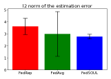
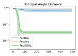
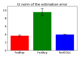
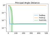
Figure S1: Small data sets - synthetic data. $b=50$ clients.

Figure S2: Small data sets - synthetic data. $b=200$ clients.

Second, we test, how the dimensionality of raw data impacts on the result. Figure S4 and Figure S4 show our results with $k\in\{5,50\}$. All others parameters are the same as before.

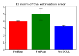
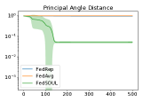
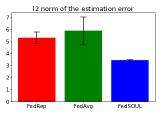
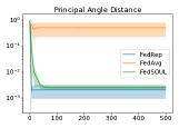
Figure S3: Small data sets - synthetic data. Raw data dimensionality is $k=50$.

Figure S4: Small data sets - synthetic data. Raw data dimensionality is $k=5$.

One more experiment we conducted is the dependence on latent dimensionality $d$. We test two options $d=2$ (as in original experiments) and $d=5$ in Figure S6 and Figure S6. Again, the more parameters we have to learn (given the same small data budget), the better Bayesian methods (i.e. FedSOUL) are better.

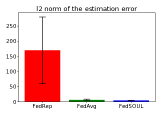
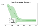
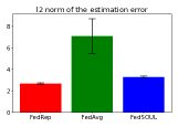
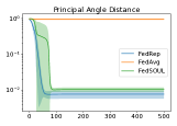
Figure S5: Small data sets - synthetic data. Latent space dimensionality is $d=5$.

Figure S6: Small data sets - synthetic data. Latent space dimensionality is $d=2$.

S3.2 Image datasets classification

In this section we provide an additional baseline for the experiments with personalization, in case we have only a few heterogeneous data. Specifically, we consider APFL (Deng et al., 2021b) which is another personalized federated learning approach. We consider CIFAR-10 dataset with 100 clients. Among these clients, there are 10, 50 or 90 which have local dataset of either 5 (one setup) or 10 (another setup). Else of size 25.

We see in Figure S7 that FedSOUL typically performs better than FedRep, but on par with APFL. It is surprizing, that APFL is a very good baseline in these type of problem, which it was not specially designed for.

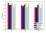
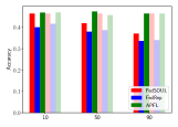
Figure S7: Small image datasets. Minimal local dataset size is 2 (top) or 5 (bottom).

S3.3 Image datasets uncertainty quantification

In this section, we provide additional experiments on image uncertainty with CIFAR-10 (in distribution) and SVHN (out of distribution) datasets. As a measure of uncertainty, we will use predictive entropy. On Figure S8, we present 4 different models among 100. In the left part of the figure we see the distribution of entropy, assigned to the in-distribution objects (validational split, but same domain as training data). In the right part we see the distribution for out-of-distribution (SVHN in our case). Contraty to MNIST vs Fashion-MNIST example, here it is not that clear that FedSOUL captures uncertainty well.

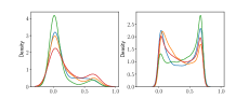
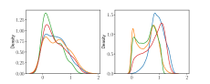
Figure S8: Out-of-distribution detection. CIFAR 10 vs SVHN. 2 classes for model (top) and 5 (bottom).

We also provide additional plots for calibration on CIFAR-10 again for two cases, when each client had 2 classes to predict or 5.

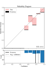
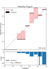
Figure S9: Reliability diagram for CIFAR10. 2 classes for model (top) and 5 (bottom).

References

- Alistarh et al. (2017) Dan Alistarh, Demjan Grubic, Jerry Li, Ryota Tomioka, and Milan Vojnovic. QSGD: Communication-efficient SGD via gradient quantization and encoding. Advances in Neural Information Processing Systems, 2017.
- Arivazhagan et al. (2019) Manoj Ghuhan Arivazhagan, Vinay Aggarwal, Aaditya Kumar Singh, and Sunav Choudhary. Federated Learning with Personalization Layers. arXiv preprint arXiv:1912.00818, 2019.
- Atchadé et al. (2017) Yves F. Atchadé, Gersende Fort, and Eric Moulines. On perturbed proximal gradient algorithms. Journal of Machine Learning Research, 18(10):1–33, 2017.
- Briggs et al. (2020) Christopher Briggs, Zhong Fan, and Peter Andras. Federated learning with hierarchical clustering of local updates to improve training on non-iid data. In 2020 International Joint Conference on Neural Networks (IJCNN), pages 1–9. IEEE, 2020.
- Bui et al. (2018) Thang D. Bui, Cuong V. Nguyen, Siddharth Swaroop, and Richard E. Turner. Partitioned Variational Inference: A unified framework encompassing federated and continual learning. arXiv preprint arXiv:1811.11206, 2018.
- Casella (1985) George Casella. An Introduction to Empirical Bayes Data Analysis. The American Statistician, 39(2):83–87, 1985.
- Chen and Chao (2020) Hong-You Chen and Wei-Lun Chao. Fedbe: Making bayesian model ensemble applicable to federated learning. arXiv preprint arXiv:2009.01974, 2020.
- Collins et al. (2021) Liam Collins, Hamed Hassani, Aryan Mokhtari, and Sanjay Shakkottai. Exploiting Shared Representations for Personalized Federated Learning. In International Conference on Machine Learning, pages 2089–2099, 2021.
- Corinzia et al. (2019) Luca Corinzia, Ami Beuret, and Joachim M. Buhmann. Variational Federated Multi-Task Learning. arXiv preprint arXiv:1906.06268, 2019.
- Dalalyan (2017) Arnak S. Dalalyan. Theoretical guarantees for approximate sampling from smooth and log-concave densities. Journal of the Royal Statistical Society, Series B, 79(3):651–676, 2017.
- De Bortoli et al. (2021) Valentin De Bortoli, Alain Durmus, Marcelo Pereyra, and Ana F. Vidal. Efficient stochastic optimisation by unadjusted Langevin Monte Carlo: Application to maximum marginal likelihood and empirical Bayesian estimation. Statistics and Computing, 31(3), 2021.
- Deng et al. (2021a) Wei Deng, Yi-An Ma, Zhao Song, Qian Zhang, and Guang Lin. On Convergence of Federated Averaging Langevin Dynamics. arXiv preprint arXiv:2112.05120, 2021a.
- Deng et al. (2021b) Yuyang Deng, Mohammad Mahdi Kamani, and Mehrdad Mahdavi. Adaptive Personalized Federated Learning, 2021b.
- Durmus and Moulines (2017) Alain Durmus and Eric Moulines. Nonasymptotic convergence analysis for the unadjusted Langevin algorithm. The Annals of Applied Probability, 27(3):1551–1587, 06 2017. doi: 10.1214/16-AAP1238.
- El Mekkaoui et al. (2021) Khaoula El Mekkaoui, Diego Mesquita, Paul Blomstedt, and Samuel Kaski. Distributed stochastic gradient MCMC for federated learning. In Conference on Uncertainty in Artificial Intelligence, 2021.
- Fallah et al. (2020) Alireza Fallah, Aryan Mokhtari, and Asuman Ozdaglar. Personalized Federated Learning with Theoretical Guarantees: A Model-Agnostic Meta-Learning Approach. In Advances in Neural Information Processing Systems, 2020.
- Gelman and Hill (2007) Andrew Gelman and Jennifer Hill. Data Analysis Using Regression and Multilevel/Hierarchical Models. Cambridge University Press, New York, 2007.
- Grant et al. (2018) Erin Grant, Chelsea Finn, Sergey Levine, Trevor Darrell, and Thomas Griffiths. Recasting Gradient-Based Meta-Learning as Hierarchical Bayes. In International Conference on Learning Representations, 2018.
- Hanzely and Richtárik (2020) Filip Hanzely and Peter Richtárik. Federated learning of a mixture of global and local models. arXiv preprint arXiv:2002.05516, 2020.
- Hanzely et al. (2020) Filip Hanzely, Slavomír Hanzely, Samuel Horváth, and Peter Richtárik. Lower bounds and optimal algorithms for personalized federated learning. arXiv preprint arXiv:2010.02372, 2020.
- Hanzely et al. (2021) Filip Hanzely, Boxin Zhao, and Mladen Kolar. Personalized federated learning: A unified framework and universal optimization techniques. arXiv: 2102.09743, February 2021.
- Hong et al. (2022) Joey Hong, Branislav Kveton, Manzil Zaheer, and Mohammad Ghavamzadeh. Hierarchical Bayesian Bandits. In Proceedings of the 25th International Conference on Artificial Intelligence and Statistics, 2022.
- Horváth et al. (2019) Samuel Horváth, Dmitry Kovalev, Konstantin Mishchenko, Sebastian Stich, and Peter Richtárik. Stochastic Distributed Learning with Gradient Quantization and Variance Reduction . arXiv preprint arXiv:1904.05115, 2019.
- Jiang et al. (2019) Yihan Jiang, Jakub Konevcnỳ, Keith Rush, and Sreeram Kannan. Improving federated learning personalization via model agnostic meta learning. arXiv preprint arXiv:1909.12488, 2019.
- Kairouz et al. (2021) Peter Kairouz, H. Brendan McMahan, Brendan Avent, Aurélien Bellet, Mehdi Bennis, Arjun Nitin Bhagoji, Kallista Bonawitz, Zachary Charles, Graham Cormode, Rachel Cummings, Rafael G. L. D’Oliveira, Hubert Eichner, Salim El Rouayheb, David Evans, Josh Gardner, Zachary Garrett, Adrià Gascón, Badih Ghazi, Phillip B. Gibbons, Marco Gruteser, Zaid Harchaoui, Chaoyang He, Lie He, Zhouyuan Huo, Ben Hutchinson, Justin Hsu, Martin Jaggi, Tara Javidi, Gauri Joshi, Mikhail Khodak, Jakub Konecný, Aleksandra Korolova, Farinaz Koushanfar, Sanmi Koyejo, Tancrède Lepoint, Yang Liu, Prateek Mittal, Mehryar Mohri, Richard Nock, Ayfer Özgür, Rasmus Pagh, Hang Qi, Daniel Ramage, Ramesh Raskar, Mariana Raykova, Dawn Song, Weikang Song, Sebastian U. Stich, Ziteng Sun, Ananda Theertha Suresh, Florian Tramèr, Praneeth Vepakomma, Jianyu Wang, Li Xiong, Zheng Xu, Qiang Yang, Felix X. Yu, Han Yu, and Sen Zhao. Advances and open problems in federated learning. Foundations and Trends in Machine Learning, 14(1–2):1–210, 2021. ISSN 1935-8237. doi: 10.1561/2200000083.
- Karimireddy et al. (2020) Sai Praneeth Karimireddy, Satyen Kale, Mehryar Mohri, Sashank Reddi, Sebastian Stich, and Ananda Theertha Suresh. SCAFFOLD: Stochastic controlled averaging for federated learning. In International Conference on Machine Learning, pages 5132–5143, 2020.
- Khodak et al. (2019) Mikhail Khodak, Maria-Florina F Balcan, and Ameet S Talwalkar. Adaptive gradient-based meta-learning methods. Advances in Neural Information Processing Systems, 32:5917–5928, 2019.
- Krizhevsky (2009) Alex Krizhevsky. Learning multiple layers of features from tiny images. Available at http://www.cs.toronto.edu/~kriz/cifar.html, 2009.
- Lavielle (2014) Marc Lavielle. Mixed Effects Models for the Population Approach: Models, Tasks, Methods and Tools. Chapman and Hall/CRC, 2014.
- LeCun et al. (2006) Yann LeCun, Sumit Chopra, Raia Hadsell, Fu Jie Huang, and et al. A tutorial on energy-based learning. In Predicting Structured Data. MIT Press, 2006.
- Li et al. (2020) Tian Li, Anit Kumar Sahu, Manzil Zaheer, Maziar Sanjabi, Ameet Talwalkar, and Virginia Smith. Federated optimization in heterogeneous networks. In I. Dhillon, D. Papailiopoulos, and V. Sze, editors, Proceedings of Machine Learning and Systems, volume 2, pages 429–450, 2020. URL https://proceedings.mlsys.org/paper/2020/file/38af86134b65d0f10fe33d30dd76442e-Paper.pdf.
- Li et al. (2021) Tian Li, Shengyuan Hu, Ahmad Beirami, and Virginia Smith. Ditto: Fair and robust federated learning through personalization. In ICML, pages 6357–6368, 2021. URL http://proceedings.mlr.press/v139/li21h.html.
- Liang et al. (2019) Paul Pu Liang, Terrance Liu, Liu Ziyin, Ruslan Salakhutdinov, and Louis-Philippe Morency. Think locally, act globally: Federated learning with local and global representations. In NeurIPS 2019 Workshop on Federated Learning, 2019.
- Liu and Simeone (2021a) Dongzhu Liu and Osvaldo Simeone. Channel-Driven Monte Carlo Sampling for Bayesian Distributed Learning in Wireless Data Centers. IEEE Journal on Selected Areas in Communications, 2021a.
- Liu and Simeone (2021b) Dongzhu Liu and Osvaldo Simeone. Wireless Federated Langevin Monte Carlo: Repurposing Channel Noise for Bayesian Sampling and Privacy. arXiv preprint arXiv:2108.07644, 2021b.
- Long (2011) Jeffrey Long. Longitudinal Data Analysis for the Behavioral Sciences Using R. Sage Publications, Inc, 2011.
- Mansour et al. (2020) Yishay Mansour, Mehryar Mohri, Jae Ro, and Ananda Theertha Suresh. Three approaches for personalization with applications to federated learning. 2020.
- McMahan et al. (2017) Brendan McMahan, Eider Moore, Daniel Ramage, Seth Hampson, and Blaise Aguera y Arcas. Communication-Efficient Learning of Deep Networks from Decentralized Data. In Aarti Singh and Jerry Zhu, editors, Proceedings of the 20th International Conference on Artificial Intelligence and Statistics, volume 54 of Proceedings of Machine Learning Research, pages 1273–1282, Fort Lauderdale, FL, USA, 20–22 Apr 2017. PMLR.
- Philippenko and Dieuleveut (2020) Constantin Philippenko and Aymeric Dieuleveut. Bidirectional compression in heterogeneous settings for distributed or federated learning with partial participation: tight convergence guarantees . arXiv preprint arXiv:2006.14591, 2020.
- Pillutla et al. (2022) Krishna Pillutla, Kshitiz Malik, Abdelrahman Mohamed, Michael Rabbat, Maziar Sanjabi, and Lin Xiao. Federated Learning with Partial Model Personalization, 2022. URL https://openreview.net/forum?id=iFf26yMjRdN.
- Plassier et al. (2021) Vincent Plassier, Maxime Vono, Alain Durmus, and Eric Moulines. DG-LMC: a turn-key and scalable synchronous distributed MCMC algorithm via Langevin Monte Carlo within Gibbs. In International Conference on Machine Learning (ICML), 2021.
- Robbins and Monro (1951) Herbert Robbins and Sutton Monro. A stochastic approximation method. Annals of Mathematical Statistics, 22(3):400–407, 09 1951. doi: 10.1214/aoms/1177729586.
- Robbins (1992) Herbert E Robbins. An empirical bayes approach to statistics. In Breakthroughs in statistics, pages 388–394. Springer, 1992.
- Robert (2001) C. P. Robert. The Bayesian Choice: from decision-theoretic foundations to computational implementation. Springer, New York, 2 edition, 2001.
- Roberts and Tweedie (1996) Gareth O. Roberts and Richard L. Tweedie. Exponential convergence of Langevin distributions and their discrete approximations. Bernoulli, 2(4):341–363, 1996.
- Singhal et al. (2021) Karan Singhal, Hakim Sidahmed, Zachary Garrett, Shanshan Wu, John Rush, and Sushant Prakash. Federated reconstruction: Partially local federated learning. In M. Ranzato, A. Beygelzimer, Y. Dauphin, P. S. Liang, and J. W. Vaughan, editors, Advances in Neural Information Processing Systems, volume 34, pages 11220–11232. Curran Associates, Inc., 2021. URL https://proceedings.neurips.cc/paper/2021/file/5d44a2b0d85aa1a4dd3f218be6422c66-Paper.pdf.
- Smith et al. (2017) Virginia Smith, Chao-Kai Chiang, Maziar Sanjabi, and Ameet Talwalkar. Federated multi-task learning. arXiv preprint arXiv:1705.10467, 2017.
- Tan et al. (2022) Alysa Ziying Tan, Han Yu, Lizhen Cui, and Qiang Yang. Towards personalized federated learning. IEEE Transactions on Neural Networks and Learning Systems, pages 1–17, 2022. doi: 10.1109/TNNLS.2022.3160699.
- Vono et al. (2022) Maxime Vono, Vincent Plassier, Alain Durmus, Aymeric Dieuleveut, and Eric Moulines. QLSD: Quantised Langevin stochastic dynamics for Bayesian federated learning. In AISTATS, 2022.
- Wang et al. (2021) Jianyu Wang, Zachary Charles, Zheng Xu, Gauri Joshi, H. Brendan McMahan, Blaise Aguera y Arcas, Maruan Al-Shedivat, Galen Andrew, Salman Avestimehr, Katharine Daly, Deepesh Data, Suhas Diggavi, Hubert Eichner, Advait Gadhikar, Zachary Garrett, Antonious M. Girgis, Filip Hanzely, Andrew Hard, Chaoyang He, Samuel Horvath, Zhouyuan Huo, Alex Ingerman, Martin Jaggi, Tara Javidi, Peter Kairouz, Satyen Kale, Sai Praneeth Karimireddy, Jakub Konecny, Sanmi Koyejo, Tian Li, Luyang Liu, Mehryar Mohri, Hang Qi, Sashank J. Reddi, Peter Richtarik, Karan Singhal, Virginia Smith, Mahdi Soltanolkotabi, Weikang Song, Ananda Theertha Suresh, Sebastian U. Stich, Ameet Talwalkar, Hongyi Wang, Blake Woodworth, Shanshan Wu, Felix X. Yu, Honglin Yuan, Manzil Zaheer, Mi Zhang, Tong Zhang, Chunxiang Zheng, Chen Zhu, and Wennan Zhu. A Field Guide to Federated Optimization. arXiv preprint arXiv:2107.06917, 2021.
- Welling and Teh (2011) Max Welling and Yee Whye Teh. Bayesian Learning via Stochastic Gradient Langevin Dynamics. In International Conference on Machine Learning, 2011.
- Yoon et al. (2018) Jaesik Yoon, Taesup Kim, Ousmane Dia, Sungwoong Kim, Yoshua Bengio, and Sungjin Ahn. Bayesian model-agnostic meta-learning. In S. Bengio, H. Wallach, H. Larochelle, K. Grauman, N. Cesa-Bianchi, and R. Garnett, editors, Advances in Neural Information Processing Systems, volume 31. Curran Associates, Inc., 2018. URL https://proceedings.neurips.cc/paper/2018/file/e1021d43911ca2c1845910d84f40aeae-Paper.pdf.