On Maximum Enstrophy Dissipation in $2$D Navier-Stokes Flows in the Limit of Vanishing Viscosity

Abstract

We consider enstrophy dissipation in two-dimensional (2D) Navier-Stokes flows and focus on how this quantity behaves in the limit of vanishing viscosity. After recalling a number of a priori estimates providing lower and upper bounds on this quantity, we state an optimization problem aimed at probing the sharpness of these estimates as functions of viscosity. More precisely, solutions of this problem are the initial conditions with fixed palinstrophy and possessing the property that the resulting 2D Navier-Stokes flows locally maximize the enstrophy dissipation over a given time window. This problem is solved numerically with an adjoint-based gradient ascent method and solutions obtained for a broad range of viscosities and lengths of the time window reveal the presence of multiple branches of local maximizers, each associated with a distinct mechanism for the amplification of palinstrophy. The dependence of the maximum enstrophy dissipation on viscosity is shown to be in quantitative agreement with the estimate due to Ciampa, Crippa & Spirito (2021), demonstrating the sharpness of this bound.

Keywords: 2D Navier-Stokes equation; enstrophy dissipation; inviscid limit; PDE-constrained optimization

1 Introduction

The physical phenomenon of “anomalous dissipation”, also referred to as the “zeroth law of turbulence”, is one of the oldest problems in turbulence [1]. This empirical law states that the energy dissipation in either forced or decaying three-dimensional (3D) turbulent flows approaches a nonzero limit as the fluid viscosity $\nu>0$ vanishes, all other flow parameters remaining fixed. There is a lot of evidence coming from both experiments and numerical simulations supporting this anomalous behavior of the energy dissipation [2, 3], but we are still far from being able to understand this problem from the mathematical point of view. The main consequence of the dissipation anomaly is an unbounded increase of velocity gradients which would in turn imply finite-time singularities in solutions of the inviscid Euler equations [4]. Similar dissipation anomalies are also known to occur in the behavior of passive scalars [5, 6].

Dissipation anomaly arises in solutions of the one-dimensional (1D) Burgers equation [7]. As regards 2D flows, the relevant question is about the behavior of the enstrophy dissipation in the limit of vanishing viscosity. The assumption that enstrophy dissipation tends to a finite (nonzero) limit as $\nu\rightarrow 0$ underlaid Batchelor’s theory of 2D turbulence [8]. However, in [9] it was argued that this quantity in fact vanishes in the inviscid limit such that Navier-Stokes flows in 2D are not subject to dissipation anomaly. This result was confirmed by rigorous analysis of the inviscid limit of 2D Navier-Stokes flows [10].

While there is no dissipation anomaly in 2D flows, it is interesting to know the worst-case (slowest) rate at which the enstrophy dissipation vanishes in the limit $\nu\rightarrow 0$. A number of theoretical results, in the form of both lower and upper bounds on the dependence of the enstrophy dissipation on $\nu$, have been established and are reviewed below. The goal of the present study is to address this question computationally by finding flows with the largest possible enstrophy dissipation as the viscosity vanishes. Such “extreme” flows will be found by solving suitably defined optimization problems with constraints in the form of partial differential equations (PDEs). This will provide insights about the sharpness of various rigorous bounds on the enstrophy dissipation in the inviscid limit. While methods of PDE optimization have had a long history in various applied areas [11], they have recently been employed to study certain fundamental problems concerning extreme behavior in fluid mechanics [12]. In particular, problems somewhat related to the subject of the present study were investigated using such techniques in [13, 14, 15].

We consider the incompressible Navier-Stokes system on a 2D periodic domain $\Omega:={\mathbb{T}}^{2}=[0,1]^{2}$ (“$:=$” means “equal to by definition”) which can be written in the vorticity form as

$$\frac{\partial\omega_{\nu}}{\partial t}+\boldsymbol{\nabla}^{\perp}\psi_{\nu}\cdot\boldsymbol{\nabla}\omega_{\nu} =\nu\boldsymbol{\Delta}\omega_{\nu} \text{in}\ \Omega\times(0,T],$$ (1a)

$$-\boldsymbol{\Delta}\psi_{\nu} =\omega_{\nu} \text{in}\ \Omega\times(0,T],$$ (1b)

$$\omega_{\nu}(t=0) =\varphi \text{in}\ \Omega,$$ (1c)

where $\omega_{\nu}$ and $\psi_{\nu}$ are the vorticity component perpendicular to the plane of motion and the corresponding streamfunction, both assumed to satisfy the periodic boundary conditions in the space variable ${\mathbf{x}}$, whereas $T>0$ is the length of the time window considered. The symbol $\varphi$ denotes the initial condition which without loss of generality is assumed to have zero mean, i.e.,

$$\int_{\Omega}\varphi({\mathbf{x}})\,d{\mathbf{x}}=0.$$ (2)

Problem (1) is known to be globally well-posed in the classical sense [16]. Its solutions are characterized by the enstrophy and palinstrophy defined, respectively, as

$$\mathcal{E}(\omega_{\nu}(\cdot,t)) :=\frac{1}{2}\,\int_{\Omega}\left|\omega_{\nu}({\mathbf{x}},t)\right|^{2}\,d{\mathbf{x}},$$ (3)

$$\mathcal{P}(\omega_{\nu}(\cdot,t)) :=\frac{1}{2}\,\int_{\Omega}\left|\boldsymbol{\nabla}\omega_{\nu}({\mathbf{x}},t)\right|^{2}\,d{\mathbf{x}},$$ (4)

which satisfy the relation

$$\frac{d\mathcal{E}(t)}{dt}=-2\nu\mathcal{P}(t).$$ (5)

We then define our main quantity of interest as

$$\chi_{\nu}(\varphi):=\frac{2\nu}{T}\int_{0}^{T}\mathcal{P}(t)\,dt={\frac{\nu}{T}}\,\int_{0}^{T}\int_{\Omega}\left|\boldsymbol{\nabla}\omega_{\nu}({\mathbf{x}},t;\varphi)\right|^{2}\,d{\mathbf{x}}dt=\frac{\mathcal{E}(0)-\mathcal{E}(T)}{T},$$ (6)

which represents the enstrophy dissipation per unit of time and will be viewed here as a function of the initial data $\varphi$.

The enstrophy dissipation (6) has been the subject of numerous estimates. We refer to the following result as a “conjecture” since it relies on some assumptions, albeit well justified, about the form of the spectrum of the solutions of (1).

Conjecture 1 (Tran & Dritschel [9])

The enstrophy dissipation in solutions of system eq. 1 is bounded above by

$$\chi_{\nu}\leq C\,\left[-\ln(\nu)\right]^{-\frac{1}{2}},$$ (7)

for some constant $C>0$ depending on the initial condition $\varphi$ and the length $T$ of the time window.

Hereafter $C=C(T)$ will denote a generic positive constant depending on the length $T$ of the considered time window with numerical values differing from one instant to another.

Bounds on enstrophy dissipation are closely related to another problem which has recently received considerable attention, namely, the question of the convergence as $\nu\rightarrow 0$ of Navier-Stokes flows to solutions of the inviscid Euler equations obtained by setting $\nu=0$ in (1a) and corresponding to the same initial condition $\varphi$. More specifically, noting (5), the fact that solutions of the inviscid Euler system conserve the enstrophy and using the reverse triangle inequality, we have

$$\chi_{\nu}(\varphi) ={\frac{\nu}{T}}\,\int_{0}^{T}\left\|\boldsymbol{\nabla}\omega_{\nu}({\mathbf{x}},t;\varphi)\right\|^{2}_{L^{2}(\Omega)}\,dt=\frac{2\nu}{T}\,\int_{0}^{T}\mathcal{P}(t)\,dt$$

$$=\frac{1}{T}\,\left[\mathcal{E}(0)-\mathcal{E}(T)\right]=\frac{1}{T}\,\left[\left\|\varphi\right\|^{2}_{L^{2}(\Omega)}-\left\|\omega_{\nu}({\mathbf{x}},T;\varphi)\right\|^{2}_{L^{2}(\Omega)}\right]$$

$$=\frac{1}{T}\,\left[\left\|\omega({\mathbf{x}},T;\varphi)\right\|^{2}_{L^{2}(\Omega)}-\left\|\omega_{\nu}({\mathbf{x}},T;\varphi)\right\|^{2}_{L^{2}(\Omega)}\right]$$

$$\leq\frac{1}{T}\,\left[\left\|\omega({\mathbf{x}},T;\varphi)\right\|_{L^{2}(\Omega)}+\left\|\omega_{\nu}({\mathbf{x}},T;\varphi)\right\|_{L^{2}(\Omega)}\right]\,\left\|\omega({\mathbf{x}},T;\varphi)-\omega_{\nu}({\mathbf{x}},T;\varphi)\right\|_{L^{2}(\Omega)}$$

$$\leq\frac{2}{T}\,\left\|\varphi\right\|_{L^{2}(\Omega)}\,\left\|\omega({\mathbf{x}},T;\varphi)-\omega_{\nu}({\mathbf{x}},T;\varphi)\right\|_{L^{2}(\Omega)},$$ (8)

where $\omega({\mathbf{x}},t):=\omega_{0}({\mathbf{x}},t)$ denotes the vorticity in the inviscid Euler flow. The above relation shows that the enstrophy dissipation over the time window $[0,T]$ can be bounded from above in terms of the difference of the vorticity fields in the viscous and inviscid flows obtained with the same initial data $\varphi$ at time $t=T$. Quantifying this difference in terms of viscosity as $\nu\rightarrow 0$ has been the subject of some recent studies. In [17] the authors showed the strong convergence of $\omega_{\nu}$ to $\omega$ as $\nu\rightarrow 0$ when $\varphi\in L^{\infty}(\Omega)$, implying the vanishing of the right-hand side (RHS) in (8). Moreover, the following estimate was established in the case when $\varphi\in L^{\infty}(\Omega)\cap B_{2,\infty}^{s}(\Omega)$ for some $s>0$, where $L^{p}$ and $B^{s}_{p,q}$ are the usual Lebesgue and Besov spaces,

$$\sup_{t\in[0,T]}\left\|\omega(\cdot,t)-\omega_{\nu}(\cdot,t)\right\|_{L^{p}(\Omega)}\leq{C}(\nu T)^{\frac{s\,e^{-2CTM}}{p(1+s\,e^{-CTM})}},$$ (9)

where $M:=\|\varphi\|_{L^{\infty}(\Omega)}$. This problem was revisited in [18] where it was proved that

$$\sup_{t\in[0,T]}\left\|\omega(\cdot,t)-\omega_{\nu}(\cdot,t)\right\|_{L^{p}(\Omega)}\leq C\,M^{1-\frac{1}{p}}\max\left\{\phi_{\varphi,p,M}(C\,\nu^{\frac{e^{-CT}}{2}}),\left(C\,\nu^{\frac{e^{-CT}}{2}}\right)^{\frac{e^{-CT}}{2p}}\right\},$$ (10)

where now $C=C(T,M)$ and $\phi_{\varphi,p,M}\>:\>{\mathbb{R}}^{+}\to{\mathbb{R}}^{+}$ is a continuous function such that $\phi_{\varphi,p,M}(0)=0$. Additional results were also obtained recently in [19, 20]. In particular, the following bound was produced in [20], which improves the rate of the weak convergence of $\omega_{\nu}$ to $\omega$ as $\nu\rightarrow 0$,

$$\sup_{t\in[0,T]}\left\|\omega(\cdot,t)-\omega_{\nu}(\cdot,t)\right\|_{\dot{H}^{-1}(\Omega)}\leq C\,\left[\frac{\nu}{|\ln(\nu)|}\right]^{\frac{e^{-CT}}{2}}.$$ (11)

We reiterate that, in the light of relation (8), inequalities (9)–(10) imply viscosity-dependent upper bounds on the enstrophy dissipation (6). This is not the case for estimate (11) as it involves a weaker norm than in (8). We will nonetheless refer to this estimate when we discuss our results in Section 4 with the hope that our findings may inspire further work on refining this estimate. On the other hand, as is evident from the following theorem, a lower bound on the maximum enstrophy dissipation is also available.

Theorem 1 (Jeong & Yoneda [21])

Let $\omega_{\nu}$ be the unique solution to eq. 1. Then, there exists initial data $\varphi$ such that the enstrophy dissipation is bounded below by

$$\chi_{\nu}\geq{C}\nu\,\left[-\ln(\nu)\right]^{\frac{1}{2}}.$$ (12)

Upper bounds on the energy and enstrophy dissipation in 2D Navier-Stokes flows in the presence of external forcing were obtained in [22].

In the present study we construct families of 2D Navier-Stokes flows which at fixed values of the viscosity $\nu$ locally maximize the enstrophy dissipation $\chi_{\nu}$ over the prescribed time window $[0,T]$. These flows are found using methods of numerical optimization to solve PDE-constrained optimization problems in which the enstrophy dissipation (6) is maximized with respect to the initial condition $\varphi$ in (1) subject to certain constraints. This is a nonconvex optimization problem and we demonstrate that for every pair $\nu$ and $T$ it admits several branches of locally maximizing solutions, each corresponding to a distinct dynamic mechanism for amplification of palinstrophy (which, as is evident from (5), drives the dissipation of enstrophy). Finally, by assessing the dependence of the maximum enstrophy dissipation determined in this way for fixed $T$ on the viscosity for decreasing values of $\nu$, we arrive at interesting new insights about the sharpness of the different a priori estimates discussed above.

The structure of the paper is as follows: in the next section we introduce the optimization problem formulated to maximize the enstrophy dissipation whereas in Section 3 we outline our gradient-based approach to finding families of local maximizers of that problem; computational results are presented in Section 4 whereas discussion and final conclusions are deferred to the last section.

2 Optimization Problem

Given a fixed viscosity $\nu$ and length $T$ of the time window, we aim to construct flows maximizing the enstrophy dissipation $\chi_{\nu}$ which will be accomplished by finding suitable optimal initial conditions ${\widecheck{\varphi}_{\nu}^{T}}$ in system (1). Since the enstrophy dissipation is given in terms of a time integral of the palinstrophy, cf. (6), we will restrict our attention to initial data with bounded palinstrophy $\mathcal{P}_{0}:=\mathcal{P}(\varphi)$, even though system (1) admits classical solutions for a much broader class of initial data [16]. We thus have the following optimization problem.

Problem 1

Given $\mathcal{P}_{0},\nu,T>0$ in system eq. 1 and the objective functional (6), find

$${\widecheck{\varphi}_{\nu}^{T}}=\underset{\varphi\in\mathcal{S}}{\operatorname*{arg\,max}}\,\chi_{\nu}(\varphi),\quad\textrm{where}\quad\mathcal{S}:=\left\{\varphi\in H^{1}(\Omega)\>:\>\int_{\Omega}\varphi({\mathbf{x}})\,d{\mathbf{x}}=0,\ \mathcal{P}(\varphi)=\mathcal{P}_{0}\right\}.$$

The Sobolev space $H^{1}(\Omega)$ is endowed with the inner product

$$\forall_{p_{1},p_{2}\in H^{1}(\Omega)}\qquad\left\langle p_{1},p_{2}\right\rangle_{H^{1}(\Omega)}=\int_{\Omega}p_{1}p_{2}+\ell^{2}\,\boldsymbol{\nabla}p_{1}\cdot\boldsymbol{\nabla}p_{2}\,d{\mathbf{x}},$$ (13)

where $\ell\in{\mathbb{R}}^{+}$ is a parameter. We note that the inner products in (13) corresponding to different values of $\ell$ are equivalent as long as $0<\ell<\infty$. However, as will be shown in the next section, the choice of the parameter $\ell$ plays an important role in the numerical solution of Problem 1. With the initial palinstrophy $\mathcal{P}_{0}$ fixed, we will find families of locally maximizing solutions of Problem 1 parameterized by $T$ for a range of viscosities $\nu$. Our approach to finding such local maximizers is described next.

3 Solution Approach

3.1 Gradient-Based Optimization

Since Problem 1 is designed to test certain subtle mathematical properties of system (1), we choose to formulate the solution approach in the continuous (“optimize-then-discretize”) setting, where the optimality conditions, constraints and gradient expressions are derived based on the original PDE before being discretized for the purpose of numerical evaluation, instead of the alternative “discretize-then-optimize” approach often used in applications [11]. We first describe the discrete gradient flow focusing on computation of the gradient of the objective functional $\chi_{\nu}(\varphi)$ with respect to the initial condition $\varphi$ and then provide some details about numerical approximations.

For given values of $\mathcal{P}_{0}$, $\nu$ and $T$, a local maximizer ${\widecheck{\varphi}_{\nu}^{T}}$ of Problem 1 can be found as ${\widecheck{\varphi}_{\nu}^{T}}=\lim_{n\rightarrow\infty}\varphi^{(n)}$ using the following iterative procedure representing a discretization of a gradient flow projected on $\mathcal{S}$

$$\varphi^{(n+1)} ={\mathbb{P}}_{\mathcal{S}}\left(\;\varphi^{(n)}+\tau_{n}\nabla\chi_{\nu}\left(\varphi^{(n)}\right)\;\right),$$ (14)

$$\varphi^{(1)} =\varphi_{0},$$

where $\varphi^{(n)}$ is an approximation of the maximizer obtained at the $n$-th iteration, $\varphi_{0}$ is the initial guess assumed to have zero mean and $\tau_{n}$ is the length of the step in the direction of the gradient $\nabla\chi_{\nu}(\varphi^{(n)})$. The palinstrophy constraint is enforced by application of a projection operator ${\mathbb{P}}_{\mathcal{S}}\;:\;H^{1}(\Omega)\rightarrow\mathcal{S}$ to be defined below.

A key step in procedure (14) is evaluation of the gradient $\nabla\chi_{\nu}(\varphi)$ of the objective functional $\chi_{\nu}(\varphi)$, cf. (6), representing its (infinite-dimensional) sensitivity to perturbations of the initial condition $\varphi$, and it is essential that the gradient be characterized by the required regularity, namely, $\nabla\chi_{\nu}(\varphi)\in H^{1}(\Omega)$. This is, in fact, guaranteed by the Riesz representation theorem [23] applicable because the Gâteaux (directional) differential $\chi_{\nu}^{\prime}(\varphi;\cdot):H^{1}(\Omega)\rightarrow{\mathbb{R}}$, defined as $\chi_{\nu}^{\prime}(\varphi;\varphi^{\prime}):=\lim_{\epsilon\rightarrow 0}\epsilon^{-1}\left[\chi_{\nu}(\varphi+\epsilon\varphi^{\prime})-\chi_{\nu}(\varphi)\right]$ for some perturbation $\varphi^{\prime}\in H^{1}(\Omega)$, is a bounded linear functional on $H^{1}(\Omega)$. The Gâteaux differential can be computed directly to give

$$\chi_{\nu}^{\prime}(\varphi;\varphi^{\prime})= {\frac{2\nu}{T}}\,\int_{0}^{T}\int_{\Omega}\boldsymbol{\nabla}\omega_{\nu}({\mathbf{x}},t;\varphi)\cdot\boldsymbol{\nabla}\omega_{\nu}^{\prime}({\mathbf{x}},t;\varphi,\varphi^{\prime})\,d{\mathbf{x}}dt$$

$$= -{\frac{2\nu}{T}}\,\int_{0}^{T}\int_{\Omega}\boldsymbol{\Delta}\omega_{\nu}({\mathbf{x}},t;\varphi)\,\omega_{\nu}^{\prime}({\mathbf{x}},t;\varphi,\varphi^{\prime})\,d{\mathbf{x}}dt,$$ (15)

where the last equality follows from integration by parts and the perturbation field $\omega_{\nu}^{\prime}=\omega_{\nu}^{\prime}({\mathbf{x}},t;\varphi,\varphi^{\prime})$ is a solution of the Navier-Stokes (1) system linearized around the trajectory corresponding to the initial data $\varphi$ [11], i.e.,

$$\mathcal{K}\begin{bmatrix}\omega_{\nu}^{\prime}\\ \psi_{\nu}^{\prime}\end{bmatrix} :=\begin{bmatrix}\frac{\partial\omega_{\nu}^{\prime}}{\partial t}+\boldsymbol{\nabla}^{\perp}\psi_{\nu}^{\prime}\cdot\boldsymbol{\nabla}\omega_{\nu}+\boldsymbol{\nabla}^{\perp}\psi_{\nu}\cdot\boldsymbol{\nabla}\omega_{\nu}^{\prime}-\nu\boldsymbol{\Delta}\omega_{\nu}^{\prime}\\ \boldsymbol{\Delta}\psi_{\nu}^{\prime}+\omega_{\nu}^{\prime}\end{bmatrix}=\begin{bmatrix}0\\ 0\end{bmatrix},$$ (16a)

$$\omega_{\nu}^{\prime}(t=0) =\varphi^{\prime},$$ (16b)

which is subject to the periodic boundary conditions and where $\psi_{\nu}^{\prime}$ is the perturbation of the stream function $\psi_{\nu}$. The Riesz representation theorem then allows us to write

$$\chi_{\nu}^{\prime}(\varphi;\varphi^{\prime})=\Big{\langle}\nabla\chi_{\nu}(\varphi),\varphi^{\prime}\Big{\rangle}_{H^{1}(\Omega)}=\Big{\langle}\nabla^{L^{2}}\chi_{\nu}(\varphi),\varphi^{\prime}\Big{\rangle}_{L^{2}(\Omega)},$$ (17)

where the $L^{2}$ inner product is obtained by setting $\ell=0$ in (13) and the Riesz representers $\nabla\chi_{\nu}(\varphi)$ and $\nabla^{L^{2}}\chi_{\nu}(\varphi)$ are the gradients of the objective functional computed with respect to the $H^{1}$ and $L^{2}$ topology, respectively. We remark that, while the $H^{1}$ gradient is used exclusively in the actual computations, cf. (14), the $L^{2}$ gradient is computed first as an intermediate step.

However, we note that expression (15) for the Gâteaux differential is not yet consistent with the Riesz form (17), because the perturbation $\varphi^{\prime}$ of the initial data (1c) does not appear in it explicitly as a factor, but is instead hidden as the initial condition in the linearized problem, cf. (16b). In order to transform (15) to the Riesz form, we introduce the adjoint states $\omega_{\nu}^{*},\psi_{\nu}^{*}\;:\;\Omega\times[0,T]\rightarrow{\mathbb{R}}$ and the following duality-pairing relation

$$\left(\mathcal{K}\begin{bmatrix}\omega_{\nu}^{\prime}\\ \psi_{\nu}^{\prime}\end{bmatrix},\begin{bmatrix}\omega_{\nu}^{*}\\ \psi_{\nu}^{*}\end{bmatrix}\right):= \int_{0}^{T}\int_{\Omega}\mathcal{K}\begin{bmatrix}\omega_{\nu}^{\prime}\\ \psi_{\nu}^{\prime}\end{bmatrix}\cdot\begin{bmatrix}\omega_{\nu}^{*}\\ \psi_{\nu}^{*}\end{bmatrix}\,d{\mathbf{x}}\,dt=0.$$ (18)

Performing integration by parts with respect to both space and time in (18) and judiciously defining the adjoint system as (also subject to the period boundary conditions)

$$\mathcal{K}^{*}\begin{bmatrix}\omega_{\nu}^{*}\\ \psi_{\nu}^{*}\end{bmatrix} :=\begin{bmatrix}-\frac{\partial\omega_{\nu}^{*}}{\partial t}-\boldsymbol{\nabla}^{\perp}\psi_{\nu}\cdot\boldsymbol{\nabla}\omega_{\nu}^{*}+\psi_{\nu}^{*}-\nu\boldsymbol{\Delta}\omega_{\nu}^{*}\\ \boldsymbol{\Delta}\psi_{\nu}^{*}-\boldsymbol{\nabla}^{\perp}\cdot(\omega_{\nu}^{*}\,\boldsymbol{\nabla}\omega_{\nu})\end{bmatrix}=\begin{bmatrix}-{\frac{2\nu}{T}}\boldsymbol{\Delta}\omega_{\nu}\\ 0\end{bmatrix},$$ (19a)

$$\omega_{\nu}^{*}(t=T) =0,$$ (19b)

we arrive at

$$\left(\mathcal{K}\begin{bmatrix}\omega_{\nu}^{\prime}\\ \psi_{\nu}^{\prime}\end{bmatrix},\begin{bmatrix}\omega_{\nu}^{*}\\ \psi_{\nu}^{*}\end{bmatrix}\right) =\left(\begin{bmatrix}\omega_{\nu}^{\prime}\\ \psi_{\nu}^{\prime}\end{bmatrix},\mathcal{K}^{*}\begin{bmatrix}\omega_{\nu}^{*}\\ \psi_{\nu}^{*}\end{bmatrix}\right)-\int_{\Omega}\varphi^{\prime}({\mathbf{x}})\,\omega_{\nu}^{*}({\mathbf{x}},0)\,d{\mathbf{x}}$$ (20)

$$=\underbrace{-{\frac{2\nu}{T}}\,\int_{0}^{T}\int_{\Omega}\omega_{\nu}^{\prime}\boldsymbol{\Delta}\omega_{\nu}\,d{\mathbf{x}}dt}_{\chi_{\nu}^{\prime}({\varphi};\varphi^{\prime})}-\int_{\Omega}\varphi^{\prime}({\mathbf{x}})\,\omega_{\nu}^{*}({\mathbf{x}},0)\,d{\mathbf{x}}=0,$$

where all boundary terms resulting from integration by parts with respect to the space variable vanish due to periodicity and one of the terms resulting from integration by parts with respect to time vanishes as well due to the terminal condition eq. 19b. Identity (20) then implies $\chi_{\nu}^{\prime}({\varphi};\varphi^{\prime})=\int_{\Omega}\,\varphi^{\prime}({\mathbf{x}})\,\omega_{\nu}^{*}({\mathbf{x}},0)\,d{\mathbf{x}}$, from which we deduce the following expression for the $L^{2}$ gradient, cf. (17),

$$\nabla^{L^{2}}\chi_{\nu}({\mathbf{x}})=\omega_{\nu}^{*}({\mathbf{x}},0).$$ (21)

We note that the $L^{2}$ gradient does not possess the regularity required to solve Problem 1. Identifying the Gâteaux differential (15) with the $H^{1}$ inner product, cf. (13), integrating by parts and using (21), we obtain the required $H^{1}$ gradient $\nabla\chi$ as a solution of the elliptic boundary-value problem

$$\left[\operatorname{Id}\,-\,\ell^{2}\,\Delta\right]\nabla\chi_{\nu}=\nabla^{L^{2}}\chi_{\nu}\qquad\text{in}\ \Omega$$ (22)

subject to the periodic boundary conditions. As shown in [24], extraction of gradients in spaces of smoother functions such as $H^{1}(\Omega)$ can be interpreted as low-pass filtering of the $L^{2}$ gradients with parameter $\ell$ acting as the cut-off length-scale. The value of $\ell$ can significantly affect the rate of convergence of the iterative procedure (14).

We define the inverse Laplacian on $\Omega$ such that it returns a zero-mean function. This ensures that the solution $\omega_{\nu}^{*}$ of the adjoint system (19) preserves the zero-mean property which is then also inherited by the $L^{2}$ and $H^{1}$ gradients, cf. (21)–(22). The projection operator in (14) is then defined in terms of the normalization (retraction)

$${\mathbb{P}}_{\mathcal{S}}(\varphi)=\sqrt{\frac{\mathcal{P}_{0}}{\mathcal{P}\left(\varphi\right)}}\,\varphi.$$ (23)

An optimal step size $\tau_{n}$ can be determined by solving the minimization problem

$$\tau_{n}=\underset{\tau>0}{\operatorname*{arg\,max}}\left\{\chi_{\nu}\left(\mathbb{P}_{\mathcal{S}}\left(\varphi^{(n)}+\tau\,\nabla\chi_{\nu}(\varphi^{(n)})\right)\right)\right\},$$ (24)

which can be interpreted as a modification of a standard line search problem with optimization performed following an arc (a geodesic) lying on the constraint manifold $\mathcal{S}$, rather than a straight line.

To summarize, a single iteration of the gradient algorithm (14) requires solution of the Navier-Stokes system (1) followed by the solution of the adjoint system (19), which is a terminal-value problem and hence needs to be integrated backward in time whereas its coefficients are determined by the solution of the Navier-Stokes system obtained before. These two solves allow one to evaluate the $L^{2}$ gradient via (21) which is then “lifted” to the space $H^{1}$ by solving (22). Finally, the approximation of the optimal initial condition ${\widecheck{\varphi}_{\nu}^{T}}$ is updated using (14) with the step size $\tau_{n}$ determined in (24). As a first initial guess $\varphi_{0}$ in eq. 14 we use the initial condition constructed in [21] and then, to ensure the maximizers ${\widecheck{\varphi}_{\nu}^{T}}$ obtained for the same viscosity $\nu$ but different lengths $T$ of the time window lie on the same maximizing branch, we use a continuation approach where the maximizer ${\widecheck{\varphi}_{\nu}^{T}}$ is employed as the initial guess $\varphi_{0}$ to compute $\widecheck{{\varphi}}_{\nu}^{T+\Delta T}$ for some sufficiently small $\Delta T$. We refer the reader to [25] for further details of the continuation approach.

3.2 Computational Approach

Both the Navier-Stokes eq. 1 and the corresponding adjoint system eq. 19 are discretized in space using a standard Fourier pseudo-spectral method. Evaluation of nonlinear products and terms with nonconstant coefficients is performed using the $2/3$ rule combined with a Gaussian filter defined by $\rho(\boldsymbol{k})=e^{-36\big{(}\frac{|\boldsymbol{k}|}{K}\big{)}^{36}}$, where $\boldsymbol{k}$ is the wavenumber, $K=\frac{2N}{3}$ and $N$ is the number of Fourier modes used in each direction [26]. Time integration is carried out using a four-step, globally third-order accurate mixed implicit/explicit Runge-Kutta scheme with low truncation error [27]. The results presented in the next section were obtained using the spatial resolutions $N=512,1024$ and the time-steps $\Delta t\approx 4.4721\times 10^{-5},2.2361\times 10^{-5},8.9443\times 10^{-6}$, with finer resolutions employed for problems with smaller values of the viscosity $\nu$. In system (22) defining the Sobolev gradients we set $\ell=1$ and a spectral method is used to solve this system. The line-search problem (24) is solved with Brent’s derivative-free algorithm [28]. Due to its large computational cost, a massively parallel implementation of the approach presented has been developed in FORTRAN 90 using the Message Passing Interface (MPI).

4 Results

In this section we present the results obtained by solving Problem 1 with $\mathcal{P}_{0}=1$ fixed and both $\nu$ and $T$ varying over a broad range of values. In addition to understanding the structure of the flows maximizing the enstrophy dissipation and how it changes when the parameters are varied, our goal is also to provide insights which of the estimates (7)–(11) best describe the behavior of the maximum enstrophy dissipation $\chi_{\nu}(\widecheck{\varphi}_{\nu}^{T})$ in the limit of vanishing viscosity.

Problem 1 is nonconvex and as such admits multiple local maximizers at least for some values of $\nu$ and $T$. Information about the six distinct local maximizers found for $\nu=2.2361\times 10^{-6}$ and $T=0.1789$ is collected in Table 1 where we show the corresponding palinstrophy evolutions $\mathcal{P}(t)$, optimal initial conditions $\widecheck{\varphi}_{\nu}^{T}({\mathbf{x}})$ and the vorticity fields realizing the maximum palinstrophy $\omega_{\nu}({\mathbf{x}},\operatorname*{arg\,max}_{0<t\leq T}\mathcal{P}(t))$. The time evolution of the vorticity fields corresponding to all six branches is visualized in Movie 1. This movie offers insights about the different physical mechanisms involving the stretching of thin vorticity filaments which are responsible for the growth of palinstrophy and hence also increased enstrophy dissipation. It is noteworthy that all these flow evolutions feature very thin filaments which however do not undergo the Kelvin-Helmholtz instability as they are stabilized by vortices also present in the flow field. Flows on branches 3 and 4, which feature multiple palinstrophy maxima, employ a mechanism similar to the continuous baker’s map to amplify the palinstrophy. Moreover, we see that, interestingly, in some cases seemingly very similar optimal initial conditions $\widecheck{\varphi}_{\nu}^{T}$ give rise to quite different flow evolutions featuring different numbers of local palinstrophy maxima (one or two) in the considered time window $[0,T]$, see, e.g., the maximizers from Branches 2 and 3 in Table 1. This makes classifying local optimizers into branches a rather difficult task and the classification presented in Table 1 is tentative only, which will however not affect the main findings of our study. Movie 2 and Movie 3 show the flow evolutions and representative palinstrophy histories corresponding to the locally optimal initial conditions $\widecheck{\varphi}_{\nu}^{T}$ obtained, respectively, on Branch 1 with $T=0.1207$ and on Branch 5 with $T=0.2683$ for five different values of the viscosity $\nu$. In both cases we see that even though the optimal initial conditions $\widecheck{\varphi}_{\nu}^{T}$ obtained for different values of $\nu$ are quite similar, qualitative changes occur in the flows evolutions as the viscosity is reduced. We attribute these changes to either possible bifurcations of the branches (understood as functions of $\nu$) or to the possibility that the flow evolutions corresponding to smaller viscosity values belong to some unclassified branch, underpinning the difficulty mentioned above.

Branch	1	2	3	4	5	6
Palinstrophy
Initial Condition
Palinstrophy Peak
Palinstrophy Peak 2	N/A	N/A			N/A	N/A

Table 1: Summary information about the local maximizers obtained by solving Problem 1 with $\nu=2.2361\times 10^{-6}$ and $T=0.1789$. The time evolution of the vorticity fields is visualized in Movie 1.

Next, in Figure 1a we show the dependence of the maximum enstrophy dissipation $\chi_{\nu}(\widecheck{\varphi}_{\nu}^{T})$ on the length $T$ of the time window for five values of viscosity spanning more than one order of magnitude. We carefully distinguish branches of distinct local maximizers, where by a “branch” we mean a family of optimal initial data $\widecheck{\varphi}_{\nu}^{T}$ parametrized by $T$ and such that the enstrophy dissipation $\chi_{\nu}(\widecheck{\varphi}_{\nu}^{T})$ changes smoothly as $T$ is varied while $\nu$ remains fixed. We remark that for certain combinations of $\nu$ and $T$ only a subset of the local maximizers described in Table 1 could be found. In Figure 1a we observe that along each branch the maximum enstrophy dissipation $\chi_{\nu}(\widecheck{\varphi}_{\nu}^{T})$ admits a well-defined maximum with respect to $T$. We add that the values of $\chi_{\nu}(\widecheck{\varphi}_{\nu}^{T})$ shown in Figure 1a are for each value of $\nu$ at least an order of magnitude larger than the enstrophy dissipation corresponding to the initial conditions constructed in [21], which realize the behavior given in (12).

As these are the quantities needed to make quantitative comparisons with estimates (7)–(11), in Figure 1b we plot the “envelopes”, defined as $\widecheck{\chi}^{T}_{\nu}:=\max_{\textrm{branches}}\chi_{\nu}(\widecheck{\varphi}_{\nu}^{T})$, of the branches obtained at fixed values of $\nu$. “Singularities” evident in these curves correspond to values of $T$ where different branches become dominant as $T$ varies.

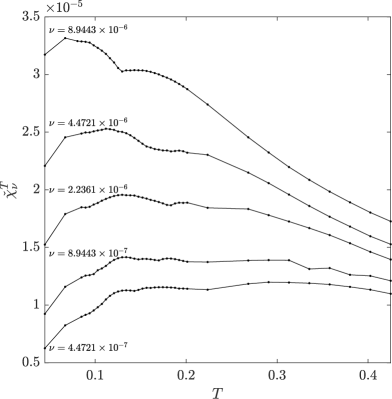
Figure 1: Dependence of (a) the maximum enstrophy dissipation $\chi_{\nu}(\widecheck{\varphi}_{\nu}^{T})$ for maximizers on the different branches, cf. Table 1, and (b) its envelope $\widecheck{\chi}^{T}_{\nu}$ on the length $T$ of the time window for different viscosities $\nu$. In panel (a) the local maximizers illustrated in Table 1 are marked with larger symbols.

Next, we move on to identify quantitative connections between the data presented in Figure 1b and estimates (7)–(11) describing the vanishing of the enstrophy dissipation in the inviscid limit $\nu\rightarrow 0$. These estimates also depend on the length $T$ of the time window, but this dependence is in some cases less explicit and we will therefore consider $T$ as a fixed parameter. We thus introduce the following ansätze

$$f_{1}(\nu) =C\,\left[-\ln(\nu)\right]^{-\frac{1}{2}},$$ (25a)

$$f_{2}(\nu) =C\,\nu^{\alpha},$$ (25b)

$$f_{3}(\nu) =C\,\left[\frac{\nu}{|\ln(\nu)|}\right]^{\alpha},$$ (25c)

$$f_{4}(\nu) =C\,\nu\,\left[-\ln(\nu)\right]^{\frac{1}{2}}$$ (25d)

motivated by the structure of the different estimates. More specifically, (25a) is the expression from Conjecture 1, cf. (7), (25b) has the general form of the upper bounds in (9)–(10), where in the latter case we only consider the second argument of the function $\max(\cdot)$ since the function $\phi_{\varphi,p,M}$ appearing in the first argument is not given explicitly enough to allow for quantitative comparisons, (25c) is motivated by the form of estimate (11) whereas (25d) is the bound from Theorem 1, cf. (12).

We want to find out which of the functions (25a)–(25d) best describes the dependence of the data shown in Figure 1b on $\nu$ for different fixed values of $T$. For each discrete value of $T$ (marked with solid symbols in Figure 1b) we determine the constant $C=C(T)$ in each of the ansatz functions (25a)–(25d) by solving the problem

$${\widetilde{C}(T)=\operatorname*{arg\,min}_{C\in{\mathbb{R}}^{+}}\mu_{i}^{T}(C),}\qquad i=1,2,3,4,$$ (26)

where the least-square error is defined as

$$\mu_{i}^{T}(C):=\frac{1}{5}\sum_{j=1}^{5}\left[\widecheck{\chi}^{T}_{\nu_{j}}-f_{i}(\nu_{j})\right]^{2}$$ (27)

with $\nu_{j}\in\{8.9443\times 10^{-6},4.4721\times 10^{-6},2.2361\times 10^{-6},8.9443\times 10^{-7},4.4721\times 10^{-7}\}$ representing the considered values of the viscosity. In addition, we note that ansatz functions (25b)–(25c) also involve a priori undefined exponents $\alpha\in(0,1)$ and to account for this fact in each of these cases solution of problem (26) is embedded in bracketing procedure which allows us to determine the exponent $\widetilde{\alpha}=\widetilde{\alpha}(T)$ producing the smallest error (27) for a given value of $T$. The bracketing procedure is performed by first determining $\mu_{i}^{T}(\widetilde{C}(T))$ for a range of discrete values of $\alpha\in[0,1]$ and then using bisection to iteratively improve the approximation of $\widetilde{\alpha}=\widetilde{\alpha}(T)$ which produces the smallest error (27). We emphasize that even though the ansätze (25a)–(25d) involve different numbers of parameters (one or two), they are all fitted to the data in Figure 1b in the same way (i.e., by adjusting $C=C(T)$), which is done independently for different discrete exponents $\alpha$ in the case of relations (25b)–(25c).

In order to assess now well the different ansatz functions (25a)–(25d) capture the dependence of the maximum enstrophy dissipation $\widecheck{\chi}^{T}_{\nu}$ on $\nu$, cf. Figure 1b, we define the ratios $\widecheck{\chi}^{T}_{\nu}/f_{i}(\nu)$, $i=1,2,3,4$, and plot them as functions of $\nu$ for different $T$ in Figures 2a–d using the values of $\widetilde{C}=\widetilde{C}(T)$ and $\widetilde{\alpha}=\widetilde{\alpha}(T)$ determined as above. Thus, if $\widecheck{\chi}^{T}_{\nu}/f_{i}(\nu)$ is close to unity over the entire range of $\nu$, this signals that the ansatz function $f_{i}(\nu)$ accurately captures the dependence of $\widecheck{\chi}^{T}_{\nu}$ on $\nu$ for the given value of $T$. We see that this is what indeed happens for $f_{2}(\nu)$ and $f_{3}(\nu)$ for most values of $T$, cf. Figures 2b,c. On the other hand, we note that relations $f_{1}(\nu)$ and $f_{4}(\nu)$, respectively, overestimate and underestimate the actual dependence of $\widecheck{\chi}^{T}_{\nu}$ on $\nu$, cf. Figures 2a,d. This observation is consistent with the fact that (25a) represents estimate (7), which is more conservative than bounds (9)–(11), and (25d) has the form of the lower bound (12).

     

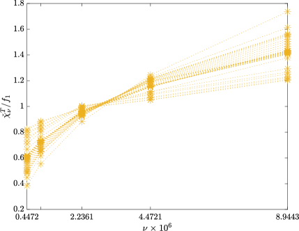
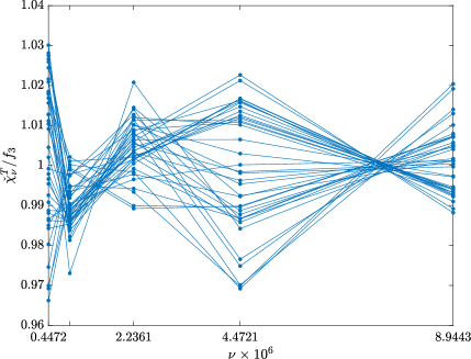
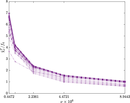
Figure 2: Dependence of (a) $\widecheck{\chi}^{T}_{\nu}/f_{1}(\nu)$, (b) $\widecheck{\chi}^{T}_{\nu}/f_{2}(\nu)$, (c) $\widecheck{\chi}^{T}_{\nu}/f_{3}(\nu)$ and (d) $\widecheck{\chi}^{T}_{\nu}/f_{4}(\nu)$, with optimal constants $\widetilde{C}=\widetilde{C}(T)$ and exponents $\widetilde{\alpha}=\widetilde{\alpha}(T)$, on the viscosity $\nu$ for different $T$.

Hereafter we will focus on the fits given in terms of ansatz functions (25b)–(25c). In order to decide which of these relations more accurately represents the dependence of $\widecheck{\chi}^{T}_{\nu}$ on $\nu$, in Figure 3 we show the corresponding mean-square errors (27) as functions of $T$. What this figure reveals is that relation $f_{2}(\nu)$ generally leads to smallers errors for shorter time windows (with $T\lessapprox 0.147$), whereas relation $f_{3}(\nu)$ tends to better predict the dependence of $\widecheck{\chi}^{T}_{\nu}$ on $\nu$ for longer time windows. Finally, the optimal exponents $\widetilde{\alpha}=\widetilde{\alpha}(T)$ determined for ansatz functions (25b)–(25c) are shown in Figure 4 where an overall decreasing trend with $T$ is evident. As regards the “dip” occurring for $0.0894\lessapprox T\lessapprox 0.1342$, we speculate that it may be the result of some branches not being captured in Figure 1a. We note that, remarkably, the dependence of the exponent $\widetilde{\alpha}$ on $T$ reveals an approximately exponential form consistent with the structure of the upper bounds in (25b)–(25c). Moreover, the limit $\lim_{T\rightarrow 0}\widetilde{\alpha}(T)$ is also quantitatively consistent with predictions of estimare (25c).

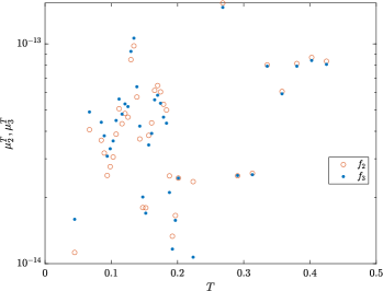
Figure 3: Dependence of the mean-square errors $\mu_{i}^{T}(\widetilde{C}(T))$, $i=2,3$, cf. eq. 27, corresponding to the fits of ansatz functions (red circles) $f_{2}(\nu)$ and (blue dots) $f_{3}(\nu)$ to $\widecheck{\chi}^{T}_{\nu}$ for different $T$.

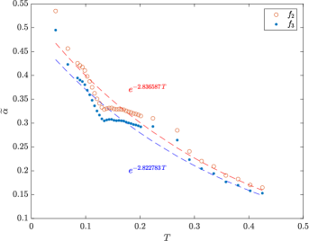
Figure 4: Dependence of the optimal exponents $\widetilde{\alpha}=\widetilde{\alpha}(T)$ in the ansatz functions (red circles) $f_{2}(\nu)$ and (blue dots) $f_{3}(\nu)$ on the length $T$ of the time window. The dashed lines represent exponential fits, in the forms indicated, to the values of $\widetilde{\alpha}=\widetilde{\alpha}(T)$ for the ansatz function (red) $f_{2}(\nu)$ and (blue) $f_{3}(\nu)$.

5 Summary and Conclusions

In this study we provide a quantitative characterization of the behaviour of the enstrophy dissipation in 2D Navier-Stokes flows in the limit of vanishing viscosity. Unlike the case of Burgers flows in 1D and Navier-Stokes flows in 3D where the energy anomaly is well documented, 2D Navier-Stokes flows are known not to exhibit anomalous behavior of enstrophy dissipation. As discussed in Introduction, the vanishing of enstrophy dissipation in the inviscid limit is subject to various estimates, some ad-hoc and some rigorous, providing lower and upper bounds on this quantity as viscosity vanishes. In our investigation we have probed the sharpness of these estimates by constructing families of Navier-Stokes flows designed to locally maximize the enstrophy dissipation subject to certain constraints. This was done by solving Problem 1 where locally optimal initial data $\widecheck{\varphi}_{\nu}^{T}$ with fixed palinstrophy $\mathcal{P}_{0}$ was found such that the corresponding flow with the given viscosity $\nu$ maximizes the enstrophy dissipation $\chi_{\nu}$ over the time window $[0,T]$. Problem 1 was solved numerically using a state-of-the-art adjoint-based gradient ascent method described in Section 3. This optimization problem is nonconvex and we have found six distinct branches of local maximizers, each associated with a different mechanism for palinstrophy amplification, cf. Table 1. As is evident from Movie 1, while in all cases palinstrophy amplification involves stretching of thin vorticity filaments, there are multiple ways to design flows maximizing this process on a periodic domain $\Omega$ and which of these different mechanisms produces the largest enstrophy dissipation depends on the value of viscosity $\nu$ and the length $T$ of the time window, cf. Figure 1a.

Branches of local maximiers found by solving Problem 1 for different values of $\nu$ and $T$ reveal how the extreme behaviour of the enstrophy dissipation they realize compares with the available estimates on this process discussed in Introduction. We conclude that the dependence of the maximum enstrophy dissipation $\widecheck{\chi}^{T}_{\nu}$ in the extreme flows we found on $\nu$ with fixed $T$ is quantitatively consistent with the upper bound in estimate (10), cf. Figure 2b, which is the sharpest estimate available to date. Remarkably, the exponential dependence of the exponent in this upper bound on $T$ is also quantitatively consistent with our results, cf. Figure 4 (we attribute the deviation from the exponential decrease evident around $T\approx 0.1342$ in this figure to the likely possibility that, despite our efforts, not all branches of maximizing solutions have been found).

As regards estimate (10), we note that it depends on the quantity $\|\widecheck{\varphi}_{\nu}^{T}\|_{L^{\infty}(\Omega)}$ (via the constant $M$). Since our optimal initial conditions are sought in the space $H^{1}(\Omega)$, we do not have an a priori control over this quantity, however, in our computations we did not find any evidence for $\|\widecheck{\varphi}_{\nu}^{T}\|_{L^{\infty}(\Omega)}$ to attain large values. Thus, these caveats notwithstanding, we conclude that estimate (10) is sharp and does not offer any room for improvement, other than perhaps a logarithmic correction analogous to the one appearing in (11). Relation (11) was found to describe the dependence of the maximum enstrophy dissipation $\widecheck{\chi}^{T}_{\nu}$ on viscosity in the limit $\nu\rightarrow 0$ with similar accuracy to estimate (10). However, we reiterate that, as discussed in Introduction, (11) does not represent a rigorous upper bound on the enstrophy dissipation. Improving this estimate, so that the $\dot{H}^{-1}(\Omega)$ norm on the left-hand side in (11) is strengthened to $L^{2}(\Omega)$, appears to be an open question in mathematical analysis.

Among other open problems, it would be interesting to better understand the bifurcation structure of the different optimal solution branches shown in Figure 1a. Another open question is what new insights about the problem considered here could be deduced based on the kinetic theory, i.e., by considering an optimization problem analogous to Problem 1 in the context of the Boltzmann equation or some of its variants. Some efforts in this direction are already underway. Finally, there is the question about what can be said about the energy dissipation anomaly in 3D Navier-Stokes flows using the approach developed in the present study.

References

- [1] U. Frisch. Turbulence. Cambridge University Press, Cambridge, 1995. The legacy of A. N. Kolmogorov.
- [2] Katepalli R. Sreenivasan. An update on the energy dissipation rate in isotropic turbulence. Physics of Fluids, 10(2):528–529, 1998.
- [3] P. K. Yeung, X. M. Zhai, and Katepalli R. Sreenivasan. Extreme events in computational turbulence. Proceedings of the National Academy of Sciences, 112(41):12633–12638, 2015.
- [4] Radu Dascaliuc and Zoran Grujić. Anomalous dissipation and energy cascade in 3D inviscid flows. Communications in Mathematical Physics, 309(3):757–770, 2012.
- [5] Katepalli R. Sreenivasan. Turbulent mixing: A perspective. Proceedings of the National Academy of Sciences, 116(37):18175–18183, 2019.
- [6] Anna L. Mazzucato. Remarks on anomalous dissipation for passive scalars. Philosophical Transactions of the Royal Society A: Mathematical, Physical and Engineering Sciences, 380(2218):20210099, 2022.
- [7] Gregory L. Eyink and Theodore D. Drivas. Spontaneous Stochasticity and Anomalous Dissipation for Burgers Equation. Journal of Statistical Physics, 158(2):386–432, Jan 2015.
- [8] G. K. Batchelor. Computation of the energy spectrum in homogeneous two‐dimensional turbulence. Phys. Fluids, 12(12):II–233–239, 1969.
- [9] CHUONG V. Tran and DAVID G. Dritschel. Vanishing enstrophy dissipation in two-dimensional Navier-Stokes turbulence in the inviscid limit. Journal of Fluid Mechanics, 559:107–116, 2006.
- [10] Milton C.Lopes Filho, Anna L. Mazzucato, and Helena J. Nussenzveig Lopes. Weak Solutions, Renormalized Solutions and Enstrophy Defects in 2D Turbulence. Archive for Rational Mechanics and Analysis, 179(3):353–387, mar 2006.
- [11] M. D. Gunzburger. Perspectives in Flow Control and Optimization. SIAM, 2003.
- [12] Bartosz Protas. Systematic search for extreme and singular behaviour in some fundamental models of fluid mechanics. Philosophical Transactions of the Royal Society A: Mathematical, Physical and Engineering Sciences, 380(2225):20210035, 2022.
- [13] D. Ayala and B. Protas. Maximum palinstrophy growth in 2D incompressible flows. Journal of Fluid Mechanics, 742:340–367, 2014.
- [14] D. Ayala and B. Protas. Vortices, maximum growth and the problem of finite-time singularity formation. Fluid Dynamics Research, 46(3):031404, 2014.
- [15] Diego Ayala, Charles R. Doering, and Thilo M. Simon. Maximum palinstrophy amplification in the two-dimensional Navier-Stokes equations. Journal of Fluid Mechanics, 837:839–857, 2018.
- [16] H. Kreiss and J. Lorenz. Initial-Boundary Value Problems and the Navier-Stokes Equations, volume 47 of Classics in Applied Mathematics. SIAM, 2004.
- [17] Peter Constantin, Theodore D. Drivas, and Tarek M. Elgindi. Inviscid Limit of Vorticity Distributions in the Yudovich Class. Communications on Pure and Applied Mathematics, 75(1):60–82, 2022.
- [18] Gennaro Ciampa, Gianluca Crippa, and Stefano Spirito. Strong convergence of the vorticity for the 2D Euler equations in the inviscid limit. Arch. Ration. Mech. Anal., 240(1):295–326, 2021.
- [19] Helena J Nussenzveig Lopes, Christian Seis, and Emil Wiedemann. On the vanishing viscosity limit for 2D incompressible flows with unbounded vorticity. Nonlinearity, 34(5):3112–3121, may 2021.
- [20] Christian Seis. A note on the vanishing viscosity limit in the Yudovich class. Canad. Math. Bull., 64(1):112–122, 2021.
- [21] In-Jee Jeong and Tsuyoshi Yoneda. Enstrophy dissipation and vortex thinning for the incompressible 2D Navier–Stokes equations. Nonlinearity, 34(4):1837–1853, feb 2021.
- [22] Alexandros Alexakis and Charles R. Doering. Energy and enstrophy dissipation in steady state 2d turbulence. Physics Letters A, 359(6):652–657, 2006.
- [23] D. Luenberger. Optimization by Vector Space Methods. John Wiley and Sons, 1969.
- [24] B. Protas, T. R. Bewley, and G. Hagen. A computational framework for the regularization of adjoint analysis in multiscale PDE systems. J. Comp. Physs., 195(1):49 – 89, 2004.
- [25] D. Ayala and B. Protas. Extreme vortex states and the growth of enstrophy in 3D incompressible flows. Journal of Fluid Mechanics, 818:772–806, 2017.
- [26] Thomas Y. Hou. Blow-up or no blow-up? A unified computational and analytic approach to 3D incompressible Euler and Navier–Stokes equations. Acta Numerica, 18:277–346, 2009.
- [27] Ryan Alimo, Daniele Cavaglieri, Pooriya Beyhaghi, and Thomas R. Bewley. Design of IMEXRK time integration schemes via Delaunay-based derivative-free optimization with nonconvex constraints and grid-based acceleration. J. Glob. Optim., 79(3):567–591, March 2021.
- [28] W. H. Press, S. A. Teukolsky, W. T. Vetterling, and B. P. Flannery. Numerical recipes. Cambridge University Press, third edition, 2007. The art of scientific computing.