Piecewise Linear Strain Cosserat Model for Soft Slender Manipulator

Haihong Li, Lingxiao Xun, Gang Zheng Haihong Li, Lingxiao Xun, Gang Zheng are in Defrost team, Inria, university of Lille, Centrale Lille, CRIStAL - Centre de Recherche en Informatique Signal et Automatique de Lille - UMR 9189, France (e-mail: haihong.li@inria.fr; lingxiao.xun@inria.fr; gang.zheng@inria.fr).
Abstract

Recently soft robotics has rapidly become a novel and promising area of research with many designs and applications due to their flexible and compliant structure. However, it is more difficult to derive the nonlinear dynamic model of such soft robots. The differential kinematics and dynamics of the soft manipulator can be formulated as a set of highly nonlinear partial differential equations (PDEs) via the classic Cosserat rod theory. In this work, we propose a discrete modeling technique named piecewise linear strain (PLS) to solve the PDEs of Cosserat-based models, based on which the associated analytic models are deduced. To validate the accuracy of the proposed Cosserat model, the static model of the conical cantilever rod under gravity as a simple example is simulated by using different discretization methods. Results indicate that PLS Cosserat model is comparable to the mechanical deformation behavior of real-world soft manipulator. Finally, a parameters identification scheme for this model is established, and the simulation as well as experimental validation demonstrate that using this method can identify the model physical parameters with high accuracy.

Index Terms:
Soft manipulator, dynamics, piecewise linear strain (PLS), Cosserat model, parameters identification

I Introduction

I-A Review of relevant literature

The soft robots, originally inspired by the structure and behavior of animal species such as octopus tentacles, elephant trunks, snakes and caterpillars [1], [2], are an emerging type of robots usually made of continuous deformable elastic elements and idealized as one-dimensional slender objects. Slender elastic rods demonstrating large deflections are increasingly prevalent not only in continuum robots, but also for the applications of the soft robots [3], [4]. Despite their potential strengths, the deformability of soft robots produces an infinite degree-of-freedom and highly coupled nonlinear system that is much tougher to model. The difficulty in modeling soft robots obviously results from falling short of tools in the field of continuum mechanics.

The beam/rod theory as a subclass of continuum mechanics provides a theoretical guidance to model numerous problems in engineering due to its generality and simplicity. The classical Euler-Bernoulli beam theory has been a widely used approach for the model analysis in the past years, but it depends on the assumption of small deflections. [5] developed a quasi-static bending model from a geometrically exact Euler–Bernoulli formulation that generalizes a sequence of soft arm designs to predict the result of design changes. Nevertheless, there exists the drawback that the model ignores bending stiffness and shearing deformation. Timoshenko beam model considering rotational and shear effects has been investigated and applied in soft robots modeling [6], [7]. In applications with large deflections, classical rod theories in nonlinear elasticity are required. The Kirchhoff rod as a geometrically nonlinear extension of the Euler-Bernoulli beam, can only describe bending and torsion deformations and be conveniently adopted to derive general models of soft continuum robots. In other words, it is a promising approach originated from the unshearable and unstretchable Cosserat rod [8], [9]. By contrast, the Cosserat rod theory is the geometrically nonlinear generalization of the Timoshenko-Reissner beam, which can model not only bending and torsion, but as well shearing and extension [10], [11], [12]. The Cosserat rod theory has been widely applied to static and dynamic modeling of soft continuum robots. The dissertation about the problems of statics, dynamics, and stability for continuum robots with slender elastic rod on the basis of Cosserat was exhaustively presented in [13]. Based on the work of [13], the authors put forward a new implicit dynamics framework for solving Cosserat partial differential equation (PDE) models applied to soft continuum robots, aiming at addressing the issue of computational difficulties [14]. [15] proposed a novel variable-strain parameterization by discretizing the continuous Cosserat rod model onto a finite set of strain basis functions for soft manipulators. Besides, a dynamic Cosserat modeling approach via the strain nonlinear parameterization has been proposed, which is numerically simple with a good accuracy and less degrees of freedom (DoFs). However, this technique leads to computational complexities owing to higher order of basis functions required when simulating significantly complicated deformation such as global buckling behaviors [16]. The pseudo-rigid body (PRB) 3R model was first established to account for the large deformation of the flexible beam subject to the tip load, and utilized to analyze the compliant mechanisms with high computational efficiency [17]. On the basis of the PRB 3R model, [18] presented a three-dimensional (3D) static modeling method with high model precision for cable-driven continuum robot for the purpose of the extension from the PRB 3R model to 3D applications.

The rod modeling frameworks to describe soft continuum robots have been laid down in light of the above reviewed beam theories. Continuous rod models have infinite-dimension states, and as such, they are significantly difficult to model and control than the discrete systems with finite DoFs. Modeling and control of soft robots for some practical applications calls for accurate and efficient models that will enable simulation of mechanical behavior, improve structural design and development of control systems. The existing alternative to yield to a finite-dimensional model of the robot can be useful for control design purposes. The mathematical foundations from the rod theories facilitate an assortment of discrete computational models. In practice, these discrete approaches allow to significantly reduce the number of DoFs of the calculated mechanical model, and simultaneously ensure the model precision. There are several typically discrete modeling techniques for soft continuum robots, which mainly contains the piecewise constant curvature (PCC) models [19], finite element models/methods (FEM) [20], [21], [22] and the piecewise constant strain (PCS) Cosserat models [23].

PCC modeling approach describes soft robots with a finite number of arcs parameterized by three quantities (i.e., (curvature, arc length, and bending plane) [19], leading to reduced-order and relatively simple mathematical models. This method has proven to be an excellent technique with a wide range of applications [24], [25], [26]. However, when considering external loads, the PCC may not be accurate owing to ignoring the presence of torsion, shear and extension. Besides, the PCC parameterization of the soft robot is independent on intrinsic variables, which results in kinematic discontinuities and singularities although they can be avoided with alternative parameterization [27], [28]. These flaws can potentially produce critical behaviors in the real-world applications.

FEM-based method which is formulated as ways of approximate solutions of PDEs was used to model physical behavior of soft robots [29], [30]. Nevertheless, to obtain exact modeling precision, this method demands that the number of nodes should tend to infinity, which negatively increases the dimension of the system and leads to a higher computation complexity. Moreover, FEM models for large-deformation 3D nonlinear elasticity always involve unnecessary computational expense when modeling long, slender arms like rod-based soft robots because general deformations of the cross sections of the model are included.

PCS Cosserat modeling technique, a discrete version of the continuous Cosserat approach [31], [32], [33], [34], was presented in [23]. It employed a finite set of piecewise constant strains with discontinuities happening at fixed points along the rod to model the deformation of the soft robots. This modeling method provides advantages to use with not only a few state variables, but also a relatively high modeling precision. As a potential and powerful alternative to the 3D FEM, the PCS Cosserat dynamic models have been increasingly applied to robots [35], [36], [37]. However, from practical point of view, with regards to the soft robots modeled through the PCS approximation, the number of sections to be divided depends on the designer of the model as a result of application-specific considerations. Remarkably, the deformation field of any certain section under external forces is not necessarily constant along the soft arm in a real scenario. The PCS is able to exactly approximate to the continuum formulation when the arm is divided into more sections, but the dimension of state variables and computational cost will highly increase, which is difficult to be used for control purposes. Consequently, a trade-off between model order reduction and accuracy should be established when soft robots modeled by the PCS approach are used for simulation and controller design.

In the past three decades, numerous model parameters identification techniques have been proposed by researchers. Several major contributions for dynamic model identification and its applications in the robotics control have been reported in [38], [39]. These studies assumed that the kinematic models were accurate, however, some typical investigations presented uncertainties of kinematic models [40], [41]. The parameters identification of static model is more obtainable than the dynamic model in practical applications since it just needs information of joint position rather than joint velocity and acceleration. The contributors of [42] derived the gravity torque by employing a Lagrangian method for a specific robot and acquired fine experimental results. [43] developed a new methodology for the joint stiffness identification of six-revolute industrial serial robots, and proposed a fast and robust procedure that can be used for the stiffness identification of the robot. In [44], the authors introduced a procedure of the static model identification towards general serial articulated manipulator and presented an application of the identified static model to validate the proposed methods. More recently, to the best of our knowledge, there remains short of the systematic approach for physical parameters identification of the static model for soft robots.

The Cosserat rod model is the closest to the mechanics of deformation of the soft robots because it can produce an exact nonlinearity in the deformations due to bending, torsion, extension, and shearing. In this paper, we first put forward a piecewise linear parameterization of the rod shape by its strain fields, namely piecewise linear strain (PLS) Cosserat model. This discrete Cosserat technique, striking a balance between accuracy, robustness and computational complexity, aims to address the lack of rigorous modeling techniques in soft robotics and develop a general framework between soft and rigid robots. Apart from the proposed modeling method, a systematic parameters identification framework based on the PLS Cosserat model for soft manipulators with arbitrary actuation manner is constructed, which is necessary and promising towards the development of model-based controller design.

I-B Contributions

The soft manipulator is modeled as a continuous assembling of cross sections moving on the midline in the 3D space via infinite rigid transformations dependent on the internal deformations. The geometrical assumption of considering no cross-section deformation allows to describe the soft arm by using ideas from the Lie group structure of rigid body motions and the other concepts from the techniques of differential geometry. In conclusion, the distinct contributions of this paper are summarized as follows:

  • *

    Propose a discrete modeling approach named PLS for large elastic deformations via the Cosserat rod theory with application to soft manipulators. The analytically integrable models involving geometric, differential kinematic and dynamic models are obtained. Simultaneously, derivation of a novel strain mode selection scheme via PLS Cosserat is provided to model different simplified beam models.

  • *

    Present a physical parameter identification strategy for the discrete Cosserat model with arbitrary actuation manner by solving a nonlinear programming (NLP) problem. Experimental setup using a cable-driven soft manipulator made of silicone indicates that the proposed method can effectively get more accurate model physical parameters. The PLS Cosserat model with the identified material parameters is capable of predicting the position of end-effector of the arm with a small relative error.

  • *

    Implement the static simulation of proposed method for soft manipulator actuated by cables, validate the precision of PLS Cosserat model, and compare the systems with different modes.

I-C Outline

The remainder of the paper is structured as follows. In Section II, the continuum models of the soft arm via the Cosserat rod on Lie group are recalled. Section III presents the detailed mathematical derivation of the novel discrete Cosserat model approach and strain mode choice scheme via Cosserat. In Section IV, a model parameters identification method based on the discrete Cosserat model is proposed. In Section V, the comparison of accuracy and computational efficiency for the discrete Cosserat models with FEM is performed through a cantilever rod simulation. In Section VI, a conical soft manipulator is designed and used to implement the model validation. Finally, the conclusion and future work are made.

II Derivation of Cosserat rod PDEs

TABLE I: Nomenclature and definitions
Symbol
Unit
Definition
X𝑋X m Arc length.
t𝑡t s Time.
𝑹(X,t)𝑹𝑋𝑡\boldsymbol{R}(X,t) Rotation matrix.
𝒖(X,t)𝒖𝑋𝑡\boldsymbol{u}(X,t) m Position vector.
𝒈(X,t)𝒈𝑋𝑡\boldsymbol{g}(X,t)
The configuration matrix 𝒈(X,t)=(𝑹𝒖𝟎T1).𝒈𝑋𝑡matrix𝑹𝒖superscript0T1\scriptsize\boldsymbol{g}(X,t)=\left(\begin{matrix}\boldsymbol{R}&\boldsymbol{u}\\ \boldsymbol{0}^{\rm T}&1\end{matrix}\right).
𝑲(X,t)𝑲𝑋𝑡\boldsymbol{K}(X,t)
1/m
Angular strain in the body frame.
𝑸(X,t)𝑸𝑋𝑡\boldsymbol{Q}(X,t)
Linear strain in the body frame.
𝛀(X,t)𝛀𝑋𝑡\boldsymbol{\Omega}(X,t)
1/s
Angular velocity in the body frame.
𝑽(X,t)𝑽𝑋𝑡\boldsymbol{V}(X,t)
m/s
Linear velocity in the body frame.
()~~\widetilde{(\cdot)}
Mapping from 3superscript3\mathbb{R}^{3} to so(3)𝑠𝑜3so(3),
e.g. 𝒂~=[0a3a2a30a1a2a10]~𝒂delimited-[]matrix0subscript𝑎3subscript𝑎2subscript𝑎30subscript𝑎1subscript𝑎2subscript𝑎10\scriptsize\widetilde{\boldsymbol{a}}=\left[\begin{matrix}0&-a_{3}&a_{2}\\ a_{3}&0&-a_{1}\\ -a_{2}&a_{1}&0\end{matrix}\right].
()^^\widehat{(\cdot)}
Mapping from 6superscript6\mathbb{R}^{6} to se(3)𝑠𝑒3se(3),
e.g. 𝝃^=(𝑲~𝑸𝟎0),𝜼^=(𝛀~𝑽𝟎0)se(3)formulae-sequence^𝝃matrix~𝑲𝑸00^𝜼matrix~𝛀𝑽00𝑠𝑒3\scriptsize\widehat{\boldsymbol{\xi}}=\left(\begin{matrix}\widetilde{\boldsymbol{K}}&\boldsymbol{Q}\\ \boldsymbol{0}&0\end{matrix}\right),\ \widehat{\boldsymbol{\eta}}=\left(\begin{matrix}\widetilde{\boldsymbol{\Omega}}&\boldsymbol{V}\\ \boldsymbol{0}&0\end{matrix}\right)\in se(3)
dXd𝑋{{\rm{d}}X} m Infinitesimal material element.
ρ𝜌\rho kg/m3 Density of material.
R(X)𝑅𝑋R(X) m Cross-sectional radius.
A(X)𝐴𝑋A(X) m2 Cross-sectional area.
E𝐸E Pa Young modulus.
ν𝜈\nu Poisson ratio.
G𝐺G
Pa
Shear modulus (For the isotropic material,
G=E/(2(1+ν))𝐺𝐸21𝜈G=E/(2(1+\nu))).
μ𝜇\mu Pa\cdots Viscosity modulus.
𝐈3subscript𝐈3\mathbf{I}_{3} 3 ×\times 3 identity matrix.
𝓙(X)𝓙𝑋\boldsymbol{\mathcal{J}}(X)
m4
Second moment of area tensor in the body
frame, 𝓙=[Jx000Jy000Jz]𝓙delimited-[]matrixsubscript𝐽𝑥000subscript𝐽𝑦000subscript𝐽𝑧\scriptsize\boldsymbol{\mathcal{J}}=\left[\begin{matrix}J_{x}&0&0\\ 0&J_{y}&0\\ 0&0&J_{z}\end{matrix}\right] (For a circular
rod, Jx=Jy+Jzsubscript𝐽𝑥subscript𝐽𝑦subscript𝐽𝑧\scriptsize J_{x}=J_{y}+J_{z}, and Jy=Jz=πR4/4subscript𝐽𝑦subscript𝐽𝑧𝜋superscript𝑅44\scriptsize J_{y}=J_{z}=\pi R^{4}/4,
Jy,Jzsubscript𝐽𝑦subscript𝐽𝑧\scriptsize J_{y},\ J_{z} are separately the second moments
of the area w.r.t. axis Y𝑌Y and Z𝑍Z, Jxsubscript𝐽𝑥J_{x} is the
polar moment of the area around the axis X𝑋X).
ad()subscriptad\rm{ad}_{(\cdot)}
The adjoint map of the Lie algebra, e.g.
ad𝝃=(𝐊~𝟎3×3𝐐~𝐊~)subscriptad𝝃matrix~𝐊subscript033~𝐐~𝐊\scriptsize\rm{ad}_{\boldsymbol{\xi}}=\left(\begin{matrix}\widetilde{\boldsymbol{K}}&\boldsymbol{0}_{3\times 3}\\ \widetilde{\boldsymbol{Q}}&\widetilde{\boldsymbol{K}}\end{matrix}\right), ad𝜼=(𝛀~𝟎3×3𝐕~𝛀~).subscriptad𝜼matrix~𝛀subscript033~𝐕~𝛀\scriptsize\ \rm{ad}_{\boldsymbol{\eta}}=\left(\begin{matrix}\widetilde{\boldsymbol{\Omega}}&\boldsymbol{0}_{3\times 3}\\ \widetilde{\boldsymbol{V}}&\widetilde{\boldsymbol{\Omega}}\end{matrix}\right).
𝓜(X)𝓜𝑋\boldsymbol{\mathcal{M}}(X)
Cross-sectional mass matrix.
𝑲tbsubscript𝑲𝑡𝑏\boldsymbol{K}_{tb}
N\cdotm
Stiffness matrix for torsion and bending,
𝑲tb=[G000E000E]𝓙(X).subscript𝑲𝑡𝑏delimited-[]matrix𝐺000𝐸000𝐸𝓙𝑋\scriptsize\boldsymbol{K}_{tb}=\left[\begin{matrix}G&0&0\\ 0&E&0\\ 0&0&E\end{matrix}\right]\boldsymbol{\mathcal{J}}(X).
𝑲essubscript𝑲𝑒𝑠\boldsymbol{K}_{es}
N
Stiffness matrix for elongation and shearing,
𝑲es=[E000G000G]A(X).subscript𝑲𝑒𝑠delimited-[]matrix𝐸000𝐺000𝐺𝐴𝑋\scriptsize\boldsymbol{K}_{es}=\left[\begin{matrix}E&0&0\\ 0&G&0\\ 0&0&G\end{matrix}\right]A(X).
𝑫tbsubscript𝑫𝑡𝑏\boldsymbol{D}_{tb}
N\cdotm2\cdots
Damping matrix for torsion and bending,
𝑫tb=[μ0003μ0003μ]𝓙(X).subscript𝑫𝑡𝑏delimited-[]matrix𝜇0003𝜇0003𝜇𝓙𝑋\scriptsize\boldsymbol{D}_{tb}=\left[\begin{matrix}\mu&0&0\\ 0&3\mu&0\\ 0&0&3\mu\end{matrix}\right]\boldsymbol{\mathcal{J}}(X).
𝑫essubscript𝑫𝑒𝑠\boldsymbol{D}_{es}
N\cdots
Damping matrix for elongation and
shearing, 𝑫es=[3μ000μ000μ]A(X).subscript𝑫𝑒𝑠delimited-[]matrix3𝜇000𝜇000𝜇𝐴𝑋\scriptsize\boldsymbol{D}_{es}=\left[\begin{matrix}3\mu&0&0\\ 0&\mu&0\\ 0&0&\mu\end{matrix}\right]A(X).
𝓟𝓟\boldsymbol{\mathcal{P}} Generalized selection matrix.
()superscript(\cdot)^{\vee} Mapping from a matrix to a vector.
Ad𝒈(X)subscriptAd𝒈𝑋{\rm{Ad}}_{\boldsymbol{g}(X)}
The matrix transforming the velocity or
acceleration twist from body frame to
inertial frame,
i.e., Ad𝒈(X)=(𝑹𝟎3×3𝒖~𝑹𝑹)6×6.subscriptAd𝒈𝑋matrix𝑹subscript033~𝒖𝑹𝑹superscript66\scriptsize{\rm{Ad}}_{\boldsymbol{g}(X)}=\left(\begin{matrix}\boldsymbol{R}&\boldsymbol{0}_{3\times 3}\\ \widetilde{\boldsymbol{u}}\boldsymbol{R}&\boldsymbol{R}\end{matrix}\right)\in\mathbb{R}^{6\times 6}.
𝒈rsubscript𝒈𝑟\boldsymbol{g}_{r}
The transformation matrix between the
inertial frame and the manipulator base
frame.
2\|\cdot\|_{2} Euclidean norm of a vector or matrix.
N𝑁N Total number of sections divided.
N¯¯𝑁\overline{N} Number of experiments.
\mathcal{L} Lagrangian function.
𝒅i(X)subscript𝒅𝑖𝑋\boldsymbol{d}_{i}(X)
mm\rm m
Local distance between the midline of soft rod
and the cable.
𝐭ci(X,t)subscript𝐭𝑐𝑖𝑋𝑡\boldsymbol{{\rm t}}_{ci}(X,t) Unit vector tangent to the cable path.

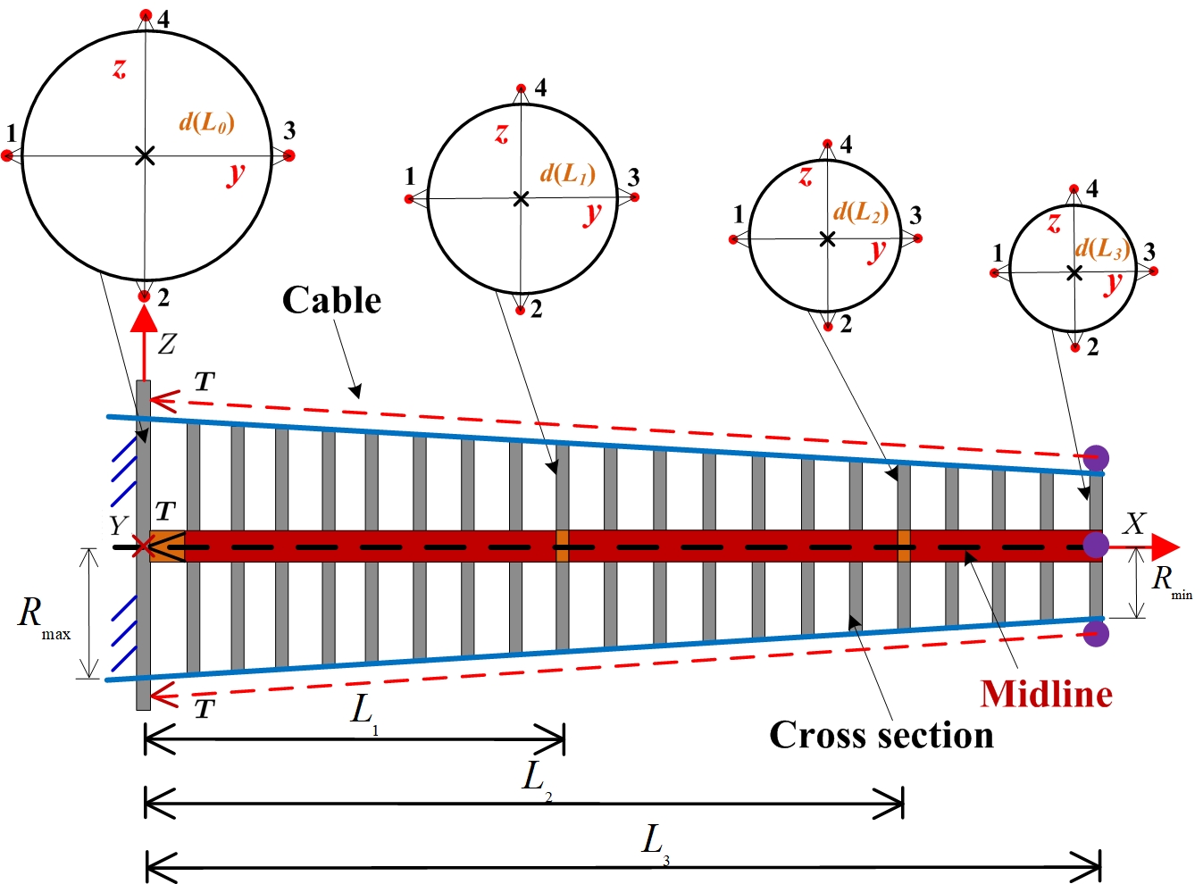
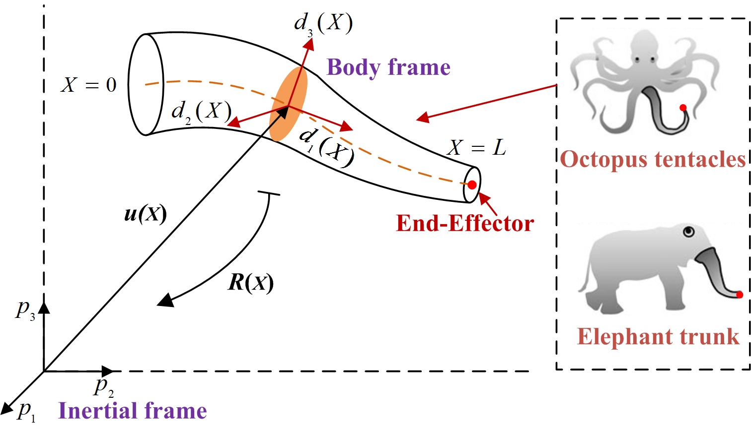
A Cosserat rod is a one-dimensional slender continuum deformable body, and each cross section of the rod is considered as an infinitesimal material element whose size and shape cannot change under external forces, as illustrated in orange part in Fig. 1. Thus, all variables of the rod can be parameterized by the reference arc length X[0,L]𝑋0𝐿X\in[0,L]\subset\mathbb{R} along the undeformed rod and by the time t𝑡t\in\mathbb{R}. For the purpose of model derivation, some variables are expressed in the inertial frame with bold small letters, but defined in the body frame attached to the cross sections as denoted by the bold capital letters. For ease of reference, the nomenclature we selected is summarized in Table I. With the aim to make the discussion of the discretization more concrete, we start by presenting the PDE system describing the Cosserat rod.
Refer to caption
Figure 1: Geometric description of a Cosserat rod and its applications.

As depicted in Fig. 1, the position field of any cross section can be represented by a centerline vector 𝒖(X,t)3𝒖𝑋𝑡superscript3\small\boldsymbol{u}(X,t)\in\mathbb{R}^{3} and an orthonormal rotation matrix 𝑹(X,t)SO(3)𝑹𝑋𝑡𝑆𝑂3\small\boldsymbol{R}(X,t)\in SO(3) with respect to the inertial frame at time t𝑡t. Hence, the homogeneous transformation matrix can be then defined as 𝒈(X,t)=(𝑹𝒖𝟎T1)SE(3)𝒈𝑋𝑡matrix𝑹𝒖superscript0T1𝑆𝐸3\small\boldsymbol{g}(X,t)=\left(\begin{matrix}\boldsymbol{R}&\boldsymbol{u}\\ \boldsymbol{0}^{\rm T}&1\end{matrix}\right)\in SE(3). For the cross section at X[0,L]𝑋0𝐿X\in[0,L], denote its strain by 𝝃(X,t)=(𝑲T,𝑸T)T6𝝃𝑋𝑡superscriptsuperscript𝑲Tsuperscript𝑸TTsuperscript6\small\boldsymbol{\xi}(X,t)=\left(\boldsymbol{K}^{\rm T},\boldsymbol{Q}^{\rm T}\right)^{\rm T}\in\mathbb{R}^{6} where 𝑲(X,t)3𝑲𝑋𝑡superscript3\small\boldsymbol{K}(X,t)\in\mathbb{R}^{3} and 𝑸(X,t)3𝑸𝑋𝑡superscript3\small\boldsymbol{Q}(X,t)\in\mathbb{R}^{3} represent respectively the angular strain (bending and torsion) and linear strain (shearing and extension), and denote its velocity by 𝜼(X,t)=(𝛀T,𝑽T)T6𝜼𝑋𝑡superscriptsuperscript𝛀Tsuperscript𝑽TTsuperscript6\small\boldsymbol{\eta}(X,t)=\left(\boldsymbol{\Omega}^{\rm T},\boldsymbol{V}^{\rm T}\right)^{\rm T}\in\mathbb{R}^{6} where 𝛀(X,t)3𝛀𝑋𝑡superscript3\small\boldsymbol{\Omega}(X,t)\in\mathbb{R}^{3} and 𝑽(X,t)3𝑽𝑋𝑡superscript3\small\boldsymbol{V}(X,t)\in\mathbb{R}^{3} respectively stand for the angular and linear velocity.

Based on the above notations, the corresponding kinematic model was derived in [36]:

𝒈=𝒈𝝃^,𝒈˙=𝒈𝜼^formulae-sequencesuperscript𝒈𝒈^𝝃˙𝒈𝒈^𝜼\small\boldsymbol{g}^{\prime}=\boldsymbol{g}\widehat{\boldsymbol{\xi}},\ \dot{\boldsymbol{g}}=\boldsymbol{g}\widehat{\boldsymbol{\eta}} (1)
𝜼=𝝃˙(X)ad𝝃(X)𝜼(X)superscript𝜼˙𝝃𝑋subscriptad𝝃𝑋𝜼𝑋\small\boldsymbol{\eta}^{\prime}=\dot{\boldsymbol{\xi}}(X)-{\rm{ad}}_{\boldsymbol{\xi}(X)}\boldsymbol{\eta}(X) (2)
𝜼˙=𝝃¨(X)ad𝝃˙(X)𝜼(X)ad𝝃(X)𝜼˙(X)superscript˙𝜼¨𝝃𝑋subscriptad˙𝝃𝑋𝜼𝑋subscriptad𝝃𝑋˙𝜼𝑋\small\dot{\boldsymbol{\eta}}^{\prime}=\ddot{\boldsymbol{\xi}}(X)-{\rm{ad}}_{\dot{\boldsymbol{\xi}}(X)}\boldsymbol{\eta}(X)-{\rm{ad}}_{\boldsymbol{\xi}(X)}\dot{{\boldsymbol{\eta}}}(X) (3)

as well as the dynamical model defined below:

𝓜𝜼˙ad𝜼T𝓜𝜼=𝓕iad𝝃T𝓕i+𝓕¯e𝓕i=𝓕ie+𝓕ia𝓜˙𝜼subscriptsuperscriptadT𝜼𝓜𝜼subscriptsuperscript𝓕𝑖subscriptsuperscriptadT𝝃subscript𝓕𝑖subscript¯𝓕𝑒subscript𝓕𝑖subscript𝓕𝑖𝑒subscript𝓕𝑖𝑎\small\begin{split}\boldsymbol{\mathcal{M}}\dot{{\boldsymbol{\eta}}}-{\rm{ad}}^{\rm{T}}_{\boldsymbol{{\eta}}}\boldsymbol{\mathcal{M}}\boldsymbol{{\eta}}&=\boldsymbol{\mathcal{F}}^{\prime}_{i}-{\rm{ad}}^{\rm{T}}_{\boldsymbol{{\xi}}}\boldsymbol{\mathcal{F}}_{i}+\overline{\boldsymbol{\mathcal{F}}}_{e}\\ \boldsymbol{\mathcal{F}}_{i}&=\boldsymbol{\mathcal{F}}_{ie}+\boldsymbol{\mathcal{F}}_{ia}\end{split} (4)

where 𝓜=ρ[diag(Jx,Jy,Jz,A,A,A)]6×6𝓜𝜌delimited-[]diagsubscript𝐽𝑥subscript𝐽𝑦subscript𝐽𝑧𝐴𝐴𝐴superscript66\small\boldsymbol{\mathcal{M}}=\rho\left[{\rm{diag}}\left(J_{x},J_{y},J_{z},A,A,A\right)\right]\in\mathbb{R}^{6\times 6}, 𝓕isubscript𝓕𝑖\small\boldsymbol{\mathcal{F}}_{i} represents the internal wrench, 𝓕¯esubscript¯𝓕𝑒\small\overline{\boldsymbol{\mathcal{F}}}_{e} is distributed external wrench, 𝓕iesubscript𝓕𝑖𝑒\small\boldsymbol{\mathcal{F}}_{ie} denotes internally elastic wrench, and 𝓕iasubscript𝓕𝑖𝑎\small\boldsymbol{\mathcal{F}}_{ia} stands for the internal wrench produced by the actuation. The above PDE (4) is defined with the boundary conditions (BCs) of the internal wrench and configurations of the tip at X=0𝑋0X=0 and X=L𝑋𝐿X=L

𝓕i(0)=𝓕e0,or𝒈(0)=𝒈0𝓕i(L)=𝓕eL,or𝒈(L)=𝒈Lformulae-sequenceformulae-sequencesubscript𝓕𝑖0subscript𝓕𝑒0or𝒈0subscript𝒈0subscript𝓕𝑖𝐿subscript𝓕𝑒𝐿or𝒈𝐿subscript𝒈𝐿\small\begin{split}\boldsymbol{\mathcal{F}}_{i}(0)&=-\boldsymbol{\mathcal{F}}_{e0},\ {\rm{or}}\ \boldsymbol{g}(0)=\boldsymbol{g}_{0}\\ \boldsymbol{\mathcal{F}}_{i}(L)&=\boldsymbol{\mathcal{F}}_{eL},\ {\rm{or}}\ \boldsymbol{g}(L)=\boldsymbol{g}_{L}\end{split} (5)

where 𝓕e0subscript𝓕𝑒0\small\boldsymbol{\mathcal{F}}_{e0} and 𝓕eLsubscript𝓕𝑒𝐿\small\boldsymbol{\mathcal{F}}_{eL} are tip external wrenches at X=0𝑋0X=0 and X=L𝑋𝐿X=L, respectively.

As for the internal elastic wrench, the Kelvin-Voigt model [45] can be adopted both for the elastic and viscous members because of the constitutive material behavior of the soft manipulator, i.e.,

𝓕ie(X)=𝚺(X)(𝝃(X)𝝃0)+𝜸(X)𝝃˙subscript𝓕𝑖𝑒𝑋𝚺𝑋𝝃𝑋subscript𝝃0𝜸𝑋˙𝝃\small\boldsymbol{\mathcal{F}}_{ie}(X)=\boldsymbol{\Sigma}(X)(\boldsymbol{{\xi}}(X)-\boldsymbol{{\xi}}_{0})+\boldsymbol{\gamma}(X)\dot{{\boldsymbol{\xi}}} (6)

with

𝚺(X)=[𝑲tb𝑲es],𝜸(X)=[𝑫tb𝑫es]formulae-sequence𝚺𝑋delimited-[]matrixsubscript𝑲𝑡𝑏missing-subexpressionmissing-subexpressionsubscript𝑲𝑒𝑠𝜸𝑋delimited-[]matrixsubscript𝑫𝑡𝑏missing-subexpressionmissing-subexpressionsubscript𝑫𝑒𝑠\small\boldsymbol{\Sigma}(X)=\left[\begin{matrix}\boldsymbol{K}_{tb}&\\ &\boldsymbol{K}_{es}\end{matrix}\right],\ \boldsymbol{\gamma}(X)=\left[\begin{matrix}\boldsymbol{D}_{tb}&\\ &\boldsymbol{D}_{es}\end{matrix}\right]

where 𝑲tb=diag(GJx(X),EJy(X),EJz(X))3×3subscript𝑲𝑡𝑏diag𝐺subscript𝐽𝑥𝑋𝐸subscript𝐽𝑦𝑋𝐸subscript𝐽𝑧𝑋superscript33\small\boldsymbol{K}_{tb}={\rm{diag}}\left(GJ_{x}(X),EJ_{y}(X),EJ_{z}(X)\right)\in\mathbb{R}^{3\times 3} and 𝑲es=diag(EA(X),GA(X),GA(X))3×3subscript𝑲𝑒𝑠diag𝐸𝐴𝑋𝐺𝐴𝑋𝐺𝐴𝑋superscript33\small\boldsymbol{K}_{es}={\rm{diag}}\left(EA(X),GA(X),GA(X)\right)\in\mathbb{R}^{3\times 3} are stiffness matrices determined by the material properties and cross-sectional geometry, 𝑫tb=diag(μJx(X),3μJy(X),3μJz(X))3×3subscript𝑫𝑡𝑏diag𝜇subscript𝐽𝑥𝑋3𝜇subscript𝐽𝑦𝑋3𝜇subscript𝐽𝑧𝑋superscript33\small\boldsymbol{D}_{tb}={\rm{diag}}\left(\mu J_{x}(X),3\mu J_{y}(X),3\mu J_{z}(X)\right)\in\mathbb{R}^{3\times 3} and 𝑫es=diag(3μA(X),μA(X),μA(X))3×3subscript𝑫𝑒𝑠diag3𝜇𝐴𝑋𝜇𝐴𝑋𝜇𝐴𝑋superscript33\small\boldsymbol{D}_{es}={\rm{diag}}\left(3\mu A(X),\mu A(X),\mu A(X)\right)\in\mathbb{R}^{3\times 3} are separately viscosity matrices for Kelvin–Voigt-type viscous damping, 𝝃0subscript𝝃0\small\boldsymbol{\xi}_{0} represents the strain related to initial configuration of the manipulator. Note that a rod cross-section does not require to be circular, and it is only needed to be slender.

The actuation wrench 𝓕iasubscript𝓕𝑖𝑎\small\boldsymbol{\mathcal{F}}_{ia} in (4) depends on the type of actuators used, and the most common actuation manners for soft manipulators are tendon and fluidic actuators. In terms of the external wrench 𝓕¯esubscript¯𝓕𝑒\small\overline{\boldsymbol{\mathcal{F}}}_{e} in (4), we can consider distributed load produced by gravity, or point load exerted by external disturbance in accordance with the actual situation.

Generally, the solution of the strong form (4) can be approximated by using many different approaches, such as implicit finite difference method [46], the shooting method [14], assumed mode method [47] and so on. In [23], by introducing the virtual displacement δϕ(X)6𝛿bold-italic-ϕ𝑋superscript6\small\delta\boldsymbol{\phi}(X)\in\mathbb{R}^{6}, the D’Alembert’s principle is used to obtain the weak form of (4), then the length space [0,L]0𝐿[0,L] was discretized into N𝑁N sections, and the strain is assumed to be constant for each section (i.e., PCS: piecewise constant strain) in order to deduce analytic formula. Clearly, such an assumption requires finely spatial discretization which yields relatively high dimensional system. Such a method can provide enough precision and work well for numerical simulation which might take time. However, PCS will be a big issue when designing model-based controllers.

To reduce the dimension of the deduced system, [16] proposed to globally approximate the strain field as 𝝃(X,t)=𝚽(X)𝒒(t)𝝃𝑋𝑡𝚽𝑋𝒒𝑡\boldsymbol{\xi}(X,t)=\boldsymbol{\Phi}(X)\boldsymbol{q}(t) where 𝚽(X)=(Φ1,Φ2,,Φn)𝚽𝑋subscriptΦ1subscriptΦ2subscriptΦ𝑛\boldsymbol{\Phi}(X)=(\Phi_{1},\Phi_{2},\cdots,\Phi_{n}) defines n𝑛n basis functions to parameterize the strain space (i.e., VS: variable strain). The advantage of VS is that the dimension of the resulted dynamical model is quite low with respect to PCS, but can provide comparable precision if the number of basis function is high enough. However, the choice of the number of basis function is highly dependent of external disturbance. For example, the external disturbance such as concentrated loads will lead to local strain mutation, and a global VS approximation method will be difficult to guarantee the local fitting precision. Moreover, all the kinematics are no more analytically integrable in contrast to PCS, but numerically reconstructed with a quaternion-based integrator. In other words, the deduced model is not anymore analytic, and will be not very friendly for control design.

In this paper, we will combine the advantages of each method, i.e., two ideas: small discretization to keep the local approximation precision (PCS), and interpolation to decrease the dimension (VS), so as to propose a piecewise linear strain (PLS) approach which is capable of obtaining the analytic formula of the model and facilitating the control design.

III Piecewise linear strain Cosserat model

In this section, the geometric (or kinematic), differential kinematic and dynamic model of the PLS Cosserat rod will be developed. Afterwards, the rod kinematics is reduced by neglecting any component of the six internal degrees of freedom (DoFs) via the PLS Cosserat model, which can effectively model Euler-Bernoulli (E-B) beam, extensible Kirchhoff (E-K) rod and Timoshenko beam, etc.

III-A Idea of PLS

Firstly, we would like to give a global picture to illustrate the difference between PCS, VS and PLS Cosserat modeling methods, and highlight the advantage of the PLS method.
Refer to caption
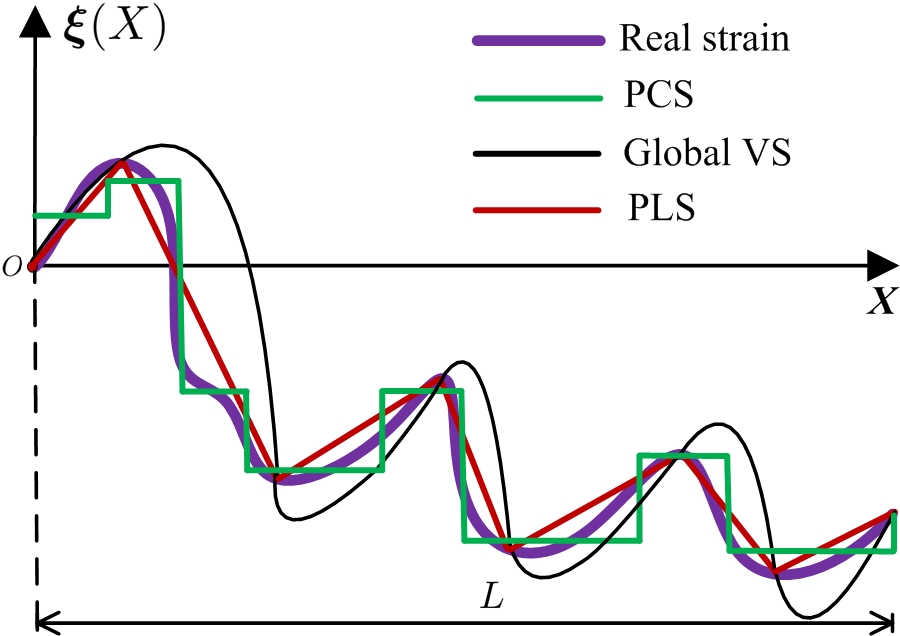
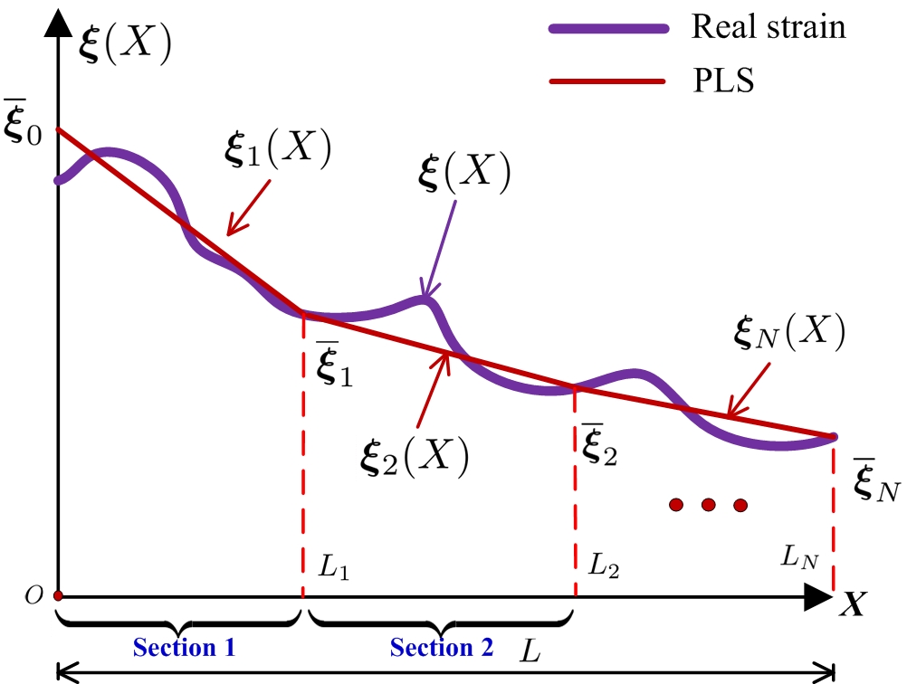
Figure 2: Sketch of comparison among VS, PCS and PLS Cosserat models with real strain.

Given an arbitrary strain field of soft body subject to external forces, as described in Fig. 2, the PCS, VS and PLS share the common objective: to approximate the real strain field as precise as possible. PCS (proposed in [23]) adopts a local approximation scheme with local constant strain assumption, while VS (proposed in [16]) uses a global approximation manner via the chosen basis functions (polynomials for example). Clearly, PCS will result in high-dimensional system in order to reach a certain precision while VS will suffer from lower precision near the local mutation region even the number of basis function is increased. Nevertheless, PLS combines both advantages of PCS and VS, and proposes to locally use a linear strain to approximate the real one. Such a scheme is able to locally approximate to the strain field of soft body compared to VS, and get much less DoFs than PCS. The sketch described in Fig. 2 intuitively demonstrates that PLS has advantages over those proposed approaches in some engineering applications, and thus provides significance for authors to carry out this work.

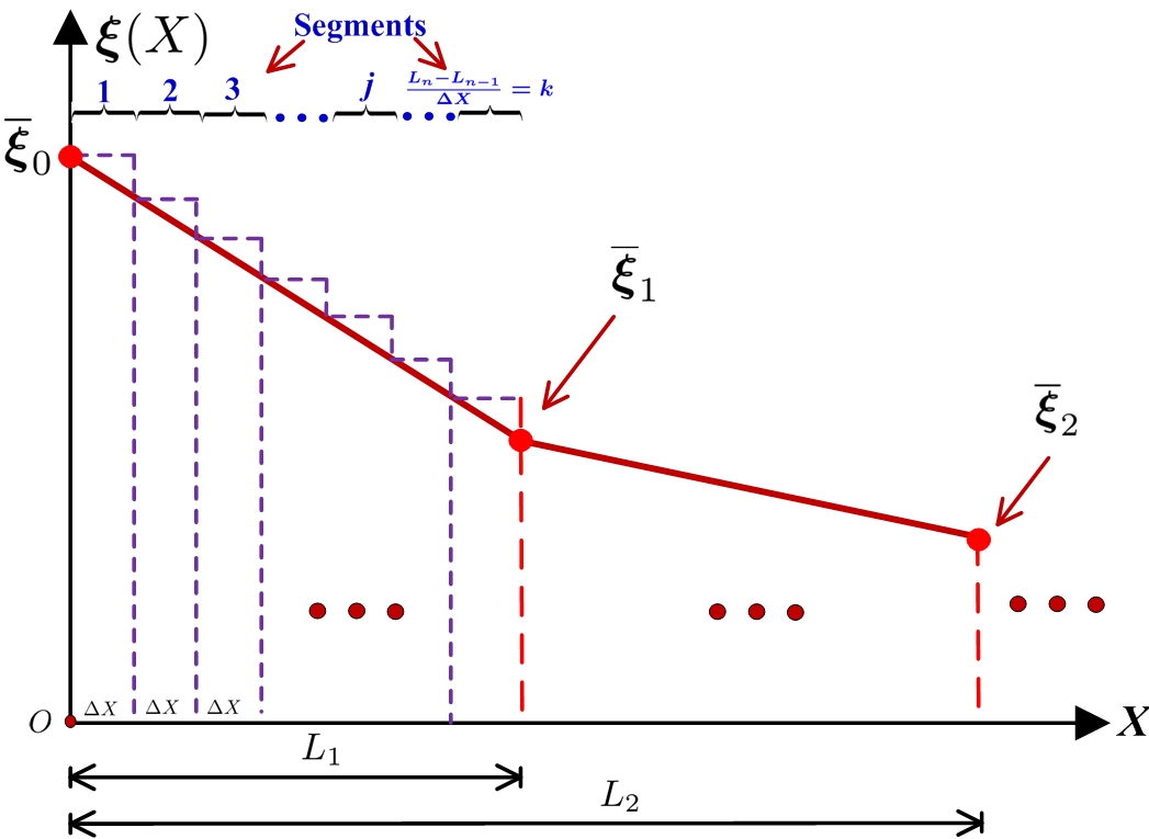
In what follows, we will focus on the PLS Cosserat modeling principle. First of all, it is noted that a “section” is defined as a unit block which is able to produce independent mechanical deformation while “segments” are a subset of one section. To put it differently, one section is made up of quite a few segments, as illustrated in Fig. 3. In view of the strain field 𝝃(X)𝝃𝑋\boldsymbol{\xi}(X) along the soft manipulator varying with the arc length X𝑋X at any moment t𝑡t, we divide the whole soft arm into N𝑁N variable length continuum sections in the form of [0,L1]0subscript𝐿1\small[0,L_{1}], [L1,L2]subscript𝐿1subscript𝐿2[L_{1},L_{2}] \cdots [LN1,LN]subscript𝐿𝑁1subscript𝐿𝑁[L_{N-1},L_{N}] (with LN=Lsubscript𝐿𝑁𝐿L_{N}=L). Generally speaking, the continuous strain field 𝝃(X)𝝃𝑋\boldsymbol{\xi}(X) is substituted for a finite set of N𝑁N continuous strain fields of the form {𝝃1(X),𝝃2(X),,𝝃N(X)}subscript𝝃1𝑋subscript𝝃2𝑋subscript𝝃𝑁𝑋\left\{\small\boldsymbol{\xi}_{1}(X),\boldsymbol{\xi}_{2}(X),\cdots,\boldsymbol{\xi}_{N}(X)\right\}. To develop this discrete Cosserat model, for any continuum section n𝑛n, we make the following two assumptions.

  • \bullet

    The strain twists 𝝃¯n1subscript¯𝝃𝑛1\small\overline{\boldsymbol{\xi}}_{n-1} and 𝝃¯nsubscript¯𝝃𝑛\small\overline{\boldsymbol{\xi}}_{n} respectively corresponds to those at the proximal and distal ends of any section n𝑛n, and other strain twists along the section n𝑛n linearly vary with X𝑋X, as shown in Fig. 3LABEL:sub@section. Based on this linear assumption, the principle of the piecewise linear strain (PLS) can be then formulated as

    𝝃n(X)=𝝃¯n1LnXLnLn1+𝝃¯nXLn1LnLn1subscript𝝃𝑛𝑋subscript¯𝝃𝑛1subscript𝐿𝑛𝑋subscript𝐿𝑛subscript𝐿𝑛1subscript¯𝝃𝑛𝑋subscript𝐿𝑛1subscript𝐿𝑛subscript𝐿𝑛1\small\boldsymbol{\xi}_{n}(X)=\overline{\boldsymbol{\xi}}_{n-1}\frac{L_{n}-X}{L_{n}-L_{n-1}}+\overline{\boldsymbol{\xi}}_{n}\frac{X-L_{n-1}}{L_{n}-L_{n-1}}

    for X[Ln1,Ln]𝑋subscript𝐿𝑛1subscript𝐿𝑛X\in[L_{n-1},L_{n}].

  • \bullet

    Since the geometric and differential kinematic models are still linear time-varying systems under the PLS assumption, the section n𝑛n is subdivided into k𝑘k (k𝑘k\in\mathbb{R}) infinitesimal segments of the form [Ln1,Ln1+ΔX],[Ln1+ΔX,Ln1+2ΔX],,[Ln1+(k1)ΔX,Ln1+kΔX]subscript𝐿𝑛1subscript𝐿𝑛1Δ𝑋subscript𝐿𝑛1Δ𝑋subscript𝐿𝑛12Δ𝑋subscript𝐿𝑛1𝑘1Δ𝑋subscript𝐿𝑛1𝑘Δ𝑋\small[L_{n-1},L_{n-1}+\Delta X],[L_{n-1}+\Delta X,L_{n-1}+2\Delta X],\cdots,[L_{n-1}+(k-1)\Delta X,L_{n-1}+k\Delta X]. In this way, the strain twists 𝝃n(X)subscript𝝃𝑛𝑋\small\boldsymbol{\xi}_{n}(X) along the segment j𝑗j remain constant, i.e., 𝝃n(X)𝝃n(Ln1+(j1)ΔX)subscript𝝃𝑛𝑋subscript𝝃𝑛subscript𝐿𝑛1𝑗1Δ𝑋\small\boldsymbol{\xi}_{n}(X)\equiv\boldsymbol{\xi}_{n}(L_{n-1}+(j-1)\Delta X), X[Ln1+(j1)ΔX,Ln1+jΔX]𝑋subscript𝐿𝑛1𝑗1Δ𝑋subscript𝐿𝑛1𝑗Δ𝑋\small{X\in[L_{n-1}+(j-1)\Delta X,L_{n-1}+j\Delta X]}. ΔXΔ𝑋\small\Delta X called one segment represents the infinitesimal distance between any adjacent cross sections, as displayed in Fig. 3LABEL:sub@segment.
Refer to caption
(a)
Refer to caption
(b)
Figure 3: Schematic illustration of the PLS Cosserat model. (a) Soft arm divided into several sections. (b) Any section subdivided into quite a few segments.

III-B PLS Cosserat: Geometric Model

Based on the PLS assumptions, for any segment j𝑗j at time t𝑡t, the system (1), (2) and (3) can be seen as liner time-invariant systems, thus they can be analytically solved. In consequence, the initial configuration, velocity or acceleration of any segment j𝑗j depend on the rightmost values of the previous segment (j1𝑗1j-1) along the section n𝑛n.

To guarantee the continuity, specifying the rightmost configuration 𝒈(Ln1)𝒈subscript𝐿𝑛1\small\boldsymbol{g}(L_{n-1}) of the section (n1)𝑛1(n-1) as the initial value of the system (1) for section n𝑛n, the rightmost configuration of any segment j𝑗j along the section n𝑛n at time t𝑡t can be recursively derived. Taking the rightmost configuration 𝒈(Ln1+jΔX)𝒈subscript𝐿𝑛1𝑗Δ𝑋\small\boldsymbol{g}(L_{n-1}+j\Delta X) of the segment j𝑗j as the initial value of system (1) for segment (j+1)𝑗1(j+1), and considering piecewise linear strain along one section, the position and orientation of any cross section at X𝑋X along the section n𝑛n at time t𝑡t analytically yields

𝒈(X)=𝒈(Ln1)(i=0j1eΔXΘni)e(XLn1jΔX)Θnj𝒈(Ln1)𝒈n(X)𝒈𝑋𝒈subscript𝐿𝑛1superscriptsubscriptproduct𝑖0𝑗1superscript𝑒Δ𝑋subscriptΘ𝑛𝑖superscript𝑒𝑋subscript𝐿𝑛1𝑗Δ𝑋subscriptΘ𝑛𝑗𝒈subscript𝐿𝑛1subscript𝒈𝑛𝑋\small\begin{split}\boldsymbol{g}(X)&=\boldsymbol{g}(L_{n-1})\left(\prod_{i=0}^{j-1}e^{\Delta X\Theta_{ni}}\right)e^{(X-L_{n-1}-j\Delta X)\Theta_{nj}}\\ &\triangleq\boldsymbol{g}(L_{n-1})\boldsymbol{g}_{n}(X)\end{split} (7)

with Θni=αni𝝃¯^n1+βni𝝃¯^nsubscriptΘ𝑛𝑖subscript𝛼𝑛𝑖subscript^¯𝝃𝑛1subscript𝛽𝑛𝑖subscript^¯𝝃𝑛\small\Theta_{ni}=\alpha_{ni}\widehat{\overline{\boldsymbol{\xi}}}_{n-1}+\beta_{ni}\widehat{\overline{\boldsymbol{\xi}}}_{n}, Θnj=αnj𝝃¯^n1+βnj𝝃¯^nsubscriptΘ𝑛𝑗subscript𝛼𝑛𝑗subscript^¯𝝃𝑛1subscript𝛽𝑛𝑗subscript^¯𝝃𝑛\small\Theta_{nj}=\alpha_{nj}\widehat{\overline{\boldsymbol{\xi}}}_{n-1}+\beta_{nj}\widehat{\overline{\boldsymbol{\xi}}}_{n}, where αni=1iΔXLnLn1subscript𝛼𝑛𝑖1𝑖Δ𝑋subscript𝐿𝑛subscript𝐿𝑛1\alpha_{ni}=1-\frac{i\Delta X}{L_{n}-L_{n-1}}, βni=iΔXLnLn1subscript𝛽𝑛𝑖𝑖Δ𝑋subscript𝐿𝑛subscript𝐿𝑛1\beta_{ni}=\frac{i\Delta X}{L_{n}-L_{n-1}}, αnj=1jΔXLnLn1subscript𝛼𝑛𝑗1𝑗Δ𝑋subscript𝐿𝑛subscript𝐿𝑛1\alpha_{nj}=1-\frac{j\Delta X}{L_{n}-L_{n-1}}, βnj=jΔXLnLn1subscript𝛽𝑛𝑗𝑗Δ𝑋subscript𝐿𝑛subscript𝐿𝑛1\beta_{nj}=\frac{j\Delta X}{L_{n}-L_{n-1}}, 𝒈n(X)subscript𝒈𝑛𝑋\small\boldsymbol{g}_{n}(X) stands for the position and orientation of any cross section at X𝑋X along the section n𝑛n w.r.t. the rightmost counterpart of the section (n1𝑛1n-1).

Intuitively, compared to PCS modeling method where 𝒈(X)𝒈𝑋\boldsymbol{g}(X) is only a function of one strain field, the model deduced from PLS in (7) depends on both 𝝃¯n1subscript¯𝝃𝑛1\small\overline{\boldsymbol{\xi}}_{n-1} and 𝝃¯nsubscript¯𝝃𝑛\small\overline{\boldsymbol{\xi}}_{n} of a certain section n𝑛n, and this is due to linear interpolation used for PLS.

III-C PLS Cosserat: Differential Kinematic Model

The differential kinematics aims to find the mapping between the velocity twist along the manipulator and the time derivatives of the system state representing deformation twist of the soft arm. Under PLS assumption, by integrating the system (2), we can then analytically obtain the velocity of each cross section at time t𝑡t (the detailed calculation of 𝜼(X)𝜼𝑋\small\boldsymbol{\eta}(X) is given in Appendix -A).

According to the Proposition 2.25 in [48] that ead𝚯superscript𝑒subscriptadsuperscript𝚯e^{{\rm{ad}}_{\boldsymbol{\Theta^{\vee}}}} is equivalent to Ade𝚯subscriptAdsuperscript𝑒𝚯{\rm{Ad}}_{e^{\boldsymbol{\Theta}}}, we know that the coefficient matrix of the velocity 𝜼(Ln1)𝜼subscript𝐿𝑛1\small\boldsymbol{\eta}(L_{n-1}) of tip at X=Ln1𝑋subscript𝐿𝑛1X=L_{n-1} of the section n𝑛n is the exponential in the adjoint representation of the Lie group transformation 𝒈n(X)subscript𝒈𝑛𝑋\small\boldsymbol{g}_{n}(X), i.e.,

e(XLn1jΔX)adΘnj(i=0j1eadΔXΘni)=Ad𝒈n(X)1superscript𝑒𝑋subscript𝐿𝑛1𝑗Δ𝑋subscriptadsuperscriptsubscriptΘ𝑛𝑗superscriptsubscriptproduct𝑖0𝑗1superscript𝑒subscriptadΔ𝑋superscriptsubscriptΘ𝑛𝑖subscriptsuperscriptAd1subscript𝒈𝑛𝑋\small e^{-(X-L_{n-1}-j\Delta X){\rm{ad}}_{\Theta_{nj}^{\vee}}}(\prod_{i=0}^{j-1}e^{-{\rm ad}_{\Delta X\Theta_{ni}^{\vee}}})={\rm{Ad}}^{-1}_{\boldsymbol{g}_{n}(X)}

Defining the coefficient matrices of 𝝃¯˙n1subscript˙¯𝝃𝑛1\small\dot{\overline{\boldsymbol{\xi}}}_{n-1} and 𝝃¯˙nsubscript˙¯𝝃𝑛\small\dot{\overline{\boldsymbol{\xi}}}_{n} separately as T𝒈n1(X)subscriptTsubscript𝒈𝑛1𝑋\small{\rm T}_{\boldsymbol{g}_{n1}(X)} and T𝒈n2(X)subscriptTsubscript𝒈𝑛2𝑋\small{\rm T}_{\boldsymbol{g}_{n2}(X)}, the analytical solution of the velocity in Appendix -A is then given by

𝜼(X)=Ad𝒈n(X)1𝜼(Ln1)+T𝒈n1(X)𝝃¯˙n1+T𝒈n2(X)𝝃¯˙n.𝜼𝑋subscriptsuperscriptAd1subscript𝒈𝑛𝑋𝜼subscript𝐿𝑛1subscriptTsubscript𝒈𝑛1𝑋subscript˙¯𝝃𝑛1subscriptTsubscript𝒈𝑛2𝑋subscript˙¯𝝃𝑛\small\boldsymbol{\eta}(X)={\rm{Ad}}^{-1}_{\boldsymbol{g}_{n}(X)}\boldsymbol{\eta}(L_{n-1})+{\rm T}_{\boldsymbol{g}_{n1}(X)}\dot{\overline{\boldsymbol{\xi}}}_{n-1}+{\rm T}_{\boldsymbol{g}_{n2}(X)}\dot{\overline{\boldsymbol{\xi}}}_{n}. (8)

with

T𝒈n1(X)=e(XLn1jΔX)adΘnji=1j[(τ=ij1eadΔXΘnτ)Ln1+(i1)ΔXLn1+iΔXe(sLn1iΔX)adΘn(i1)αn(i1)ds]+Ln1+jΔXXe(Xs)adΘnjαnjds,subscriptTsubscript𝒈𝑛1𝑋superscript𝑒𝑋subscript𝐿𝑛1𝑗Δ𝑋subscriptadsuperscriptsubscriptΘ𝑛𝑗superscriptsubscript𝑖1𝑗delimited-[]superscriptsubscriptproduct𝜏𝑖𝑗1superscript𝑒subscriptadΔ𝑋superscriptsubscriptΘ𝑛𝜏superscriptsubscriptsubscript𝐿𝑛1𝑖1Δ𝑋subscript𝐿𝑛1𝑖Δ𝑋superscript𝑒𝑠subscript𝐿𝑛1𝑖Δ𝑋subscriptadsuperscriptsubscriptΘ𝑛𝑖1subscript𝛼𝑛𝑖1d𝑠superscriptsubscriptsubscript𝐿𝑛1𝑗Δ𝑋𝑋superscript𝑒𝑋𝑠subscriptadsuperscriptsubscriptΘ𝑛𝑗subscript𝛼𝑛𝑗differential-d𝑠\small\begin{split}{\rm{T}}_{\boldsymbol{g}_{n1}(X)}&=e^{-(X-L_{n-1}-j\Delta X){\rm{ad}}_{\Theta_{nj}^{\vee}}}\sum_{i=1}^{j}\Big{[}\Big{(}\prod_{\tau=i}^{j-1}e^{-{\rm ad}_{\Delta X\Theta_{n\tau}^{\vee}}}\Big{)}\\ &\quad\int_{L_{n-1}+(i-1)\Delta X}^{L_{n-1}+i\Delta X}e^{(s-L_{n-1}-i\Delta X){\rm ad}_{\Theta_{n(i-1)}^{\vee}}}\alpha_{n(i-1)}{\rm d}s\Big{]}\\ &\quad+\int_{L_{n-1}+j\Delta X}^{X}e^{-(X-s){\rm{ad}}_{\Theta_{nj}^{\vee}}}\alpha_{nj}{\rm d}s,\end{split}
T𝒈n2(X)=e(XLn1jΔX)adΘnji=1j[(τ=ij1eadΔXΘnτ)Ln1+(i1)ΔXLn1+iΔXe(sLn1iΔX)adΘn(i1)βn(i1)ds]+Ln1+jΔXXe(Xs)adΘnjβnjds,subscriptTsubscript𝒈𝑛2𝑋superscript𝑒𝑋subscript𝐿𝑛1𝑗Δ𝑋subscriptadsuperscriptsubscriptΘ𝑛𝑗superscriptsubscript𝑖1𝑗delimited-[]superscriptsubscriptproduct𝜏𝑖𝑗1superscript𝑒subscriptadΔ𝑋superscriptsubscriptΘ𝑛𝜏superscriptsubscriptsubscript𝐿𝑛1𝑖1Δ𝑋subscript𝐿𝑛1𝑖Δ𝑋superscript𝑒𝑠subscript𝐿𝑛1𝑖Δ𝑋subscriptadsuperscriptsubscriptΘ𝑛𝑖1subscript𝛽𝑛𝑖1d𝑠superscriptsubscriptsubscript𝐿𝑛1𝑗Δ𝑋𝑋superscript𝑒𝑋𝑠subscriptadsuperscriptsubscriptΘ𝑛𝑗subscript𝛽𝑛𝑗differential-d𝑠\small\begin{split}{\rm{T}}_{\boldsymbol{g}_{n2}(X)}&=e^{-(X-L_{n-1}-j\Delta X){\rm{ad}}_{\Theta_{nj}^{\vee}}}\sum_{i=1}^{j}\Big{[}\Big{(}\prod_{\tau=i}^{j-1}e^{-{\rm ad}_{\Delta X\Theta_{n\tau}^{\vee}}}\Big{)}\\ &\quad\int_{L_{n-1}+(i-1)\Delta X}^{L_{n-1}+i\Delta X}e^{(s-L_{n-1}-i\Delta X){\rm ad}_{\Theta_{n(i-1)}^{\vee}}}\beta_{n(i-1)}{\rm d}s\Big{]}\\ &\quad+\int_{L_{n-1}+j\Delta X}^{X}e^{-(X-s){\rm{ad}}_{\Theta_{nj}^{\vee}}}\beta_{nj}{\rm d}s,\end{split}

where the symbol \vee is an operator about mapping a matrix into a vector.

From (8), if we know the strain twists (𝝃¯n1subscript¯𝝃𝑛1\small\overline{\boldsymbol{\xi}}_{n-1} and 𝝃¯nsubscript¯𝝃𝑛\small\overline{\boldsymbol{\xi}}_{n}) and strain twists rates (𝝃¯˙n1subscript˙¯𝝃𝑛1\small\dot{\overline{\boldsymbol{\xi}}}_{n-1} and 𝝃¯˙nsubscript˙¯𝝃𝑛\small\dot{\overline{\boldsymbol{\xi}}}_{n}) of tips at X=Ln1𝑋subscript𝐿𝑛1X=L_{n-1} and X=Ln𝑋subscript𝐿𝑛X=L_{n}, the velocity of any cross section at X𝑋X and time t𝑡t along the section n𝑛n can be recursively derived.

Due to the same reason, the acceleration 𝜼˙(X)˙𝜼𝑋\dot{\boldsymbol{\eta}}(X) of any cross section at X𝑋X of the section n𝑛n along the soft manipulator at time t𝑡t can be analytically computed. Considering linearly variable strain twists along a certain section n𝑛n and using the property of Lie algebra that admn=adnmsubscriptad𝑚𝑛subscriptad𝑛𝑚{\rm{ad}}_{m}n=-{\rm{ad}}_{n}m holds for any m𝑚m and n𝑛n, the system (3) can be analytically solved, and the detailed derivation is given in Appendix -A. For the sake of simplicity, this analytical solution is re-formulated below in the compact way as

𝜼˙(X)=Ad𝒈n(X)1𝜼˙(Ln1)+AD𝒈n1(X)𝝃¯˙n1+AD𝒈n2(X)𝝃¯˙n+T𝒈n1(X)𝝃¯¨n1+T𝒈n2(X)𝝃¯¨n.˙𝜼𝑋subscriptsuperscriptAd1subscript𝒈𝑛𝑋˙𝜼subscript𝐿𝑛1subscriptADsubscript𝒈𝑛1𝑋subscript˙¯𝝃𝑛1subscriptADsubscript𝒈𝑛2𝑋subscript˙¯𝝃𝑛subscriptTsubscript𝒈𝑛1𝑋subscript¨¯𝝃𝑛1subscriptTsubscript𝒈𝑛2𝑋subscript¨¯𝝃𝑛\small\begin{split}\dot{\boldsymbol{\eta}}(X)&={\rm{Ad}}^{-1}_{\boldsymbol{g}_{n}(X)}\dot{\boldsymbol{\eta}}(L_{n-1})+{\rm AD}_{\boldsymbol{g}_{n1}(X)}\dot{\overline{\boldsymbol{\xi}}}_{n-1}\\ &\quad+{\rm AD}_{\boldsymbol{g}_{n2}(X)}\dot{\overline{\boldsymbol{\xi}}}_{n}+{\rm T}_{\boldsymbol{g}_{n1}(X)}\ddot{\overline{\boldsymbol{\xi}}}_{n-1}+{\rm T}_{\boldsymbol{g}_{n2}(X)}\ddot{\overline{\boldsymbol{\xi}}}_{n}.\end{split} (9)

with

AD=𝒈n1(X)e(XLn1jΔX)adΘnji=1j[(τ=ij1eadΔXΘnτ)Ln1+(i1)ΔXLn1+iΔXe(sLn1iΔX)adΘn(i1)ad𝜼(s)αn(i1)ds]+Ln1+jΔXXe(Xs)adΘnjad𝜼(s)αnjds,\small\begin{split}{\rm{AD}}&{}_{\boldsymbol{g}_{n1}(X)}=e^{-(X-L_{n-1}-j\Delta X){\rm{ad}}_{\Theta_{nj}^{\vee}}}\sum_{i=1}^{j}\Big{[}\Big{(}\prod_{\tau=i}^{j-1}e^{-{\rm ad}_{\Delta X\Theta_{n\tau}^{\vee}}}\Big{)}\\ &\int_{L_{n-1}+(i-1)\Delta X}^{L_{n-1}+i\Delta X}e^{(s-L_{n-1}-i\Delta X){\rm ad}_{\Theta_{n(i-1)}^{\vee}}}{\rm{ad}}_{\boldsymbol{\eta}(s)}\alpha_{n(i-1)}{\rm d}s\Big{]}\\ &+\int_{L_{n-1}+j\Delta X}^{X}e^{-(X-s){\rm{ad}}_{\Theta_{nj}^{\vee}}}{\rm{ad}}_{\boldsymbol{\eta}(s)}\alpha_{nj}{\rm d}s,\end{split}

and

AD=𝒈n2(X)e(XLn1jΔX)adΘnji=1j[(τ=ij1eadΔXΘnτ)Ln1+(i1)ΔXLn1+iΔXe(sLn1iΔX)adΘn(i1)ad𝜼(s)βn(i1)ds]+Ln1+jΔXXe(Xs)adΘnjad𝜼(s)βnjds.\small\begin{split}{\rm{AD}}&{}_{\boldsymbol{g}_{n2}(X)}=e^{-(X-L_{n-1}-j\Delta X){\rm{ad}}_{\Theta_{nj}^{\vee}}}\sum_{i=1}^{j}\Big{[}\Big{(}\prod_{\tau=i}^{j-1}e^{-{\rm ad}_{\Delta X\Theta_{n\tau}^{\vee}}}\Big{)}\\ &\int_{L_{n-1}+(i-1)\Delta X}^{L_{n-1}+i\Delta X}e^{(s-L_{n-1}-i\Delta X){\rm ad}_{\Theta_{n(i-1)}^{\vee}}}{\rm{ad}}_{\boldsymbol{\eta}(s)}\beta_{n(i-1)}{\rm d}s\Big{]}\\ &+\int_{L_{n-1}+j\Delta X}^{X}e^{-(X-s){\rm{ad}}_{\Theta_{nj}^{\vee}}}{\rm{ad}}_{\boldsymbol{\eta}(s)}\beta_{nj}{\rm d}s.\end{split}

Thus, we can use (9) to calculate the acceleration of all cross sections along the section n𝑛n if knowing strain twists (𝝃¯n1subscript¯𝝃𝑛1\small\overline{\boldsymbol{\xi}}_{n-1} and 𝝃¯nsubscript¯𝝃𝑛\small\overline{\boldsymbol{\xi}}_{n}), strain twist rates (𝝃¯˙n1subscript˙¯𝝃𝑛1\small\dot{\overline{\boldsymbol{\xi}}}_{n-1} and 𝝃¯˙nsubscript˙¯𝝃𝑛\small\dot{\overline{\boldsymbol{\xi}}}_{n}) and rates of strain twist rate (𝝃¯¨n1subscript¨¯𝝃𝑛1\small\ddot{\overline{\boldsymbol{\xi}}}_{n-1} and 𝝃¯¨nsubscript¨¯𝝃𝑛\small\ddot{\overline{\boldsymbol{\xi}}}_{n}) of tips at X=Ln1𝑋subscript𝐿𝑛1X=L_{n-1} and X=Ln𝑋subscript𝐿𝑛X=L_{n}.

The relation between the velocity twist 𝜼(X)𝜼𝑋\small\boldsymbol{\eta}(X) along the robot and the strain twists (𝝃¯n1subscript¯𝝃𝑛1\small\overline{\boldsymbol{\xi}}_{n-1} and 𝝃¯nsubscript¯𝝃𝑛\small\overline{\boldsymbol{\xi}}_{n}), and another relation between the acceleration twist 𝜼˙(X)˙𝜼𝑋\small\dot{\boldsymbol{\eta}}(X) and the strain twists (𝝃¯n1subscript¯𝝃𝑛1\small\overline{\boldsymbol{\xi}}_{n-1} and 𝝃¯nsubscript¯𝝃𝑛\small\overline{\boldsymbol{\xi}}_{n}) as well as the rate of strain twists (𝝃¯˙n1subscript˙¯𝝃𝑛1\small\dot{\overline{\boldsymbol{\xi}}}_{n-1} and 𝝃¯˙nsubscript˙¯𝝃𝑛\small\dot{\overline{\boldsymbol{\xi}}}_{n}) of the tips for the section n𝑛n ought to be illustrated in order to derive the subsequent PLS Cosserat dynamic model. Applying (8) from base to tip for all cross sections along the soft manipulator in the chain, we can obtain the mapping as the geometric Jacobian which is an essential tool to describe the differential kinematics and dynamics of the PLS Cosserat model. Defining 𝑺()6×6subscript𝑺superscript66\small\boldsymbol{S}_{(\cdot)}\in\mathbb{R}^{6\times 6} and 𝑺˙()6×6subscript˙𝑺superscript66\small\dot{\boldsymbol{S}}_{(\cdot)}\in\mathbb{R}^{6\times 6} as the components of the Jacobian matrix and its partial derivative in time t𝑡t, the structural form of Jacobian and its derivative over the length of the soft arm can be separately expressed as 𝑱(𝝃¯0,𝝃¯1,,𝝃¯N1,𝝃¯N,X)=[𝑺0𝑺1𝑺2𝑺3𝑺N]6×6(N+1)𝑱subscript¯𝝃0subscript¯𝝃1subscript¯𝝃𝑁1subscript¯𝝃𝑁𝑋delimited-[]subscript𝑺0subscript𝑺1subscript𝑺2subscript𝑺3subscript𝑺𝑁superscript66𝑁1\small\boldsymbol{J}(\overline{\boldsymbol{\xi}}_{0},\overline{\boldsymbol{\xi}}_{1},\cdots,\overline{\boldsymbol{\xi}}_{N-1},\overline{\boldsymbol{\xi}}_{N},X)=[\boldsymbol{S}_{0}\quad\boldsymbol{S}_{1}\quad\boldsymbol{S}_{2}\quad\boldsymbol{S}_{3}\cdots\boldsymbol{S}_{N}]\in\mathbb{R}^{6\times 6(N+1)}, and 𝑱˙(𝝃¯0,𝝃¯1,,𝝃¯N,𝝃¯˙0,𝝃¯˙1,,𝝃¯˙N1,𝝃¯˙N,X)=[𝑺˙0𝑺˙1𝑺˙2𝑺˙3𝑺˙N]6×6(N+1)˙𝑱subscript¯𝝃0subscript¯𝝃1subscript¯𝝃𝑁subscript˙¯𝝃0subscript˙¯𝝃1subscript˙¯𝝃𝑁1subscript˙¯𝝃𝑁𝑋delimited-[]subscript˙𝑺0subscript˙𝑺1subscript˙𝑺2subscript˙𝑺3subscript˙𝑺𝑁superscript66𝑁1\small\dot{\boldsymbol{J}}(\overline{\boldsymbol{\xi}}_{0},\overline{\boldsymbol{\xi}}_{1},\cdots,\overline{\boldsymbol{\xi}}_{N},\dot{\overline{\boldsymbol{\xi}}}_{0},\dot{\overline{\boldsymbol{\xi}}}_{1},\cdots,\dot{\overline{\boldsymbol{\xi}}}_{N-1},\dot{\overline{\boldsymbol{\xi}}}_{N},X)=[\dot{\boldsymbol{S}}_{0}\quad\dot{\boldsymbol{S}}_{1}\quad\dot{\boldsymbol{S}}_{2}\quad\dot{\boldsymbol{S}}_{3}\cdots\dot{\boldsymbol{S}}_{N}]\in\mathbb{R}^{6\times 6(N+1)}.

The geometric Jacobian represents the relationship between the velocity twists of the soft manipulator and the time derivative of the deformations. The joint position vector 𝒒=[𝝃¯0T𝝃¯1T𝝃¯2T𝝃¯NT]T6(N+1)𝒒superscriptdelimited-[]matrixsubscriptsuperscript¯𝝃T0subscriptsuperscript¯𝝃T1subscriptsuperscript¯𝝃T2subscriptsuperscript¯𝝃T𝑁Tsuperscript6𝑁1\small\boldsymbol{q}=[\begin{matrix}\overline{\boldsymbol{\xi}}^{\rm T}_{0}&\overline{\boldsymbol{\xi}}^{\rm T}_{1}&\overline{\boldsymbol{\xi}}^{\rm T}_{2}&\cdots&\overline{\boldsymbol{\xi}}^{\rm T}_{N}\end{matrix}]^{\rm T}\in\mathbb{R}^{6(N+1)} composed of strain twists of all linear interpolation nodes is introduced, and the manipulator like a cantilever rod selected as an objective is fixed to a mobile base (the velocity twist of the fixed end 𝜼(0)=𝟎𝜼00\boldsymbol{\eta}(0)=\boldsymbol{0}). As a result, the discrete model of velocity (8) is globally equivalent to

𝜼(X)=𝑱(𝒒,X)𝒒˙.𝜼𝑋𝑱𝒒𝑋˙𝒒\small\boldsymbol{\eta}(X)=\boldsymbol{J}(\boldsymbol{q},X)\dot{\boldsymbol{q}}. (10)

where the analytical formula of 𝑱(𝒒,X)𝑱𝒒𝑋\boldsymbol{J}(\boldsymbol{q},X) can be found in (34) of Appendix -B. Finally, by taking the derivative of (10) with respect to time t𝑡t, the acceleration twist 𝜼˙(X)˙𝜼𝑋\dot{\boldsymbol{\eta}}(X) arrives at

𝜼˙(X)=𝑱(𝒒,X)𝒒¨+𝑱˙(𝒒,𝒒˙,X)𝒒˙.˙𝜼𝑋𝑱𝒒𝑋¨𝒒˙𝑱𝒒˙𝒒𝑋˙𝒒\small\dot{\boldsymbol{\eta}}(X)=\boldsymbol{J}(\boldsymbol{q},X)\ddot{\boldsymbol{q}}+\dot{\boldsymbol{J}}(\boldsymbol{q},\dot{\boldsymbol{q}},X)\dot{\boldsymbol{q}}. (11)

and the analytical formula of 𝑱˙(𝒒,𝒒˙,X)˙𝑱𝒒˙𝒒𝑋\dot{\boldsymbol{J}}(\boldsymbol{q},\dot{\boldsymbol{q}},X) is detailed in (35) of Appendix -B.

We would like to emphasize that, compared to PCS method, the deduced Jacobian matrix and its derivative in time are significantly different, and this is due to the linear interpolation scheme used in PLS method.

III-D PLS Cosserat: Dynamic model

In order to deduce PLS Cosserat rod dynamics model corresponding to the PDE (4), we introduce the relation between virtual displacement and the state vector δϕ(X)=𝑱(𝒒,X)𝓟δ𝒒a𝛿bold-italic-ϕ𝑋𝑱𝒒𝑋𝓟𝛿subscript𝒒𝑎\small\delta\boldsymbol{\phi}(X)=\boldsymbol{J}(\boldsymbol{q},X)\boldsymbol{\mathcal{P}}\delta\boldsymbol{q}_{a} based on the fact that the strain twist 𝝃¯Nsubscript¯𝝃𝑁\small\overline{\boldsymbol{\xi}}_{N} of the free end of the soft arm is constrained by the boundary condition. Substituting differential kinematics models (10) and (11) into the weak form of (4), a nonlinear ODE can be then obtained. Considering that the resulted ODE holds for δ𝒒aT𝟎for-all𝛿subscriptsuperscript𝒒T𝑎0\small\forall\delta\boldsymbol{q}^{\rm T}_{a}\neq\boldsymbol{0}, the generalized dynamics for the PLS Cosserat model yields

(𝓟T0LN𝑱T𝓜𝑱dX)𝒒¨[𝓟T0LN𝑱T(ad𝑱𝒒˙T𝓜𝑱𝓜𝑱˙)dX]𝒒˙=𝓟T0LN𝑱T(𝓕iead𝝃T𝓕ie)dX+𝓟T0LN𝑱T𝓕¯edX+𝓟T0LN𝑱T(𝓕iaad𝝃T𝓕ia)dXsuperscript𝓟Tsuperscriptsubscript0subscript𝐿𝑁superscript𝑱T𝓜𝑱differential-d𝑋¨𝒒delimited-[]superscript𝓟Tsuperscriptsubscript0subscript𝐿𝑁superscript𝑱TsubscriptsuperscriptadT𝑱˙𝒒𝓜𝑱𝓜˙𝑱differential-d𝑋˙𝒒superscript𝓟Tsuperscriptsubscript0subscript𝐿𝑁superscript𝑱Tsubscriptsuperscript𝓕𝑖𝑒subscriptsuperscriptadT𝝃subscript𝓕𝑖𝑒differential-d𝑋superscript𝓟Tsuperscriptsubscript0subscript𝐿𝑁superscript𝑱Tsubscript¯𝓕𝑒differential-d𝑋superscript𝓟Tsuperscriptsubscript0subscript𝐿𝑁superscript𝑱Tsubscriptsuperscript𝓕𝑖𝑎subscriptsuperscriptadT𝝃subscript𝓕𝑖𝑎differential-d𝑋\scriptsize\begin{split}&\left(\boldsymbol{\mathcal{P}}^{\rm T}\int_{0}^{L_{N}}\boldsymbol{J}^{\rm T}\boldsymbol{\mathcal{M}}\boldsymbol{J}{\rm d}X\right)\ddot{\boldsymbol{q}}-\left[\boldsymbol{\mathcal{P}}^{\rm T}\int_{0}^{L_{N}}\boldsymbol{J}^{\rm T}\left({\rm ad}^{\rm{T}}_{\boldsymbol{J}\dot{\boldsymbol{q}}}\boldsymbol{\mathcal{M}}\boldsymbol{J}-\boldsymbol{\mathcal{M}}\dot{{\boldsymbol{J}}}\right){\rm d}X\right]\dot{\boldsymbol{q}}\\ &=\boldsymbol{\mathcal{P}}^{\rm T}\int_{0}^{L_{N}}\boldsymbol{J}^{\rm T}\left(\boldsymbol{\mathcal{F}}^{\prime}_{ie}-{\rm{ad}}^{\rm{T}}_{\boldsymbol{{\xi}}}\boldsymbol{\mathcal{F}}_{ie}\right){\rm d}X+\boldsymbol{\mathcal{P}}^{\rm T}\int_{0}^{L_{N}}\boldsymbol{J}^{\rm T}\overline{\boldsymbol{\mathcal{F}}}_{e}{\rm d}X\\ &\quad+\boldsymbol{\mathcal{P}}^{\rm T}\int_{0}^{L_{N}}\boldsymbol{J}^{\rm T}\left(\boldsymbol{\mathcal{F}}^{\prime}_{ia}-{\rm{ad}}^{\rm{T}}_{\boldsymbol{{\xi}}}\boldsymbol{\mathcal{F}}_{ia}\right){\rm d}X\end{split} (16)

with 𝓟=[𝐈6N×6N𝟎6×6N]𝓟delimited-[]matrixsubscript𝐈6𝑁6𝑁subscript066𝑁\small\boldsymbol{\mathcal{P}}=\left[\begin{matrix}\mathbf{I}_{6N\times 6N}\\ \mathbf{0}_{6\times 6N}\end{matrix}\right], and δ𝒒a=[δ𝝃¯0Tδ𝝃¯1Tδ𝝃¯N1T]T6N𝛿subscript𝒒𝑎superscriptdelimited-[]matrix𝛿subscriptsuperscript¯𝝃T0𝛿subscriptsuperscript¯𝝃T1𝛿subscriptsuperscript¯𝝃T𝑁1Tsuperscript6𝑁\small\delta\boldsymbol{q}_{a}=\left[\begin{matrix}\delta\overline{\boldsymbol{\xi}}^{\rm T}_{0}&\delta\overline{\boldsymbol{\xi}}^{\rm T}_{1}&\cdots&\delta\overline{\boldsymbol{\xi}}^{\rm T}_{N-1}\end{matrix}\right]^{\rm T}\in\mathbb{R}^{6N}.

Let us define the following generalized coefficient matrices and wrenches from (16):

  • \bullet

    𝓟T0LN𝑱T𝓜𝑱dX=𝑴(𝒒)superscript𝓟Tsuperscriptsubscript0subscript𝐿𝑁superscript𝑱T𝓜𝑱differential-d𝑋𝑴𝒒\small\boldsymbol{\mathcal{P}}^{\rm T}\int_{0}^{L_{N}}\boldsymbol{J}^{\rm T}\boldsymbol{\mathcal{M}}\boldsymbol{J}{\rm d}X=\boldsymbol{M}(\boldsymbol{q}), the 6N×6(N+1)6𝑁6𝑁16N\times 6(N+1) mass matrix.

  • \bullet

    𝓟T0LN𝑱T(ad𝑱𝒒˙T𝓜𝑱𝓜𝑱˙)dX=𝑪(𝒒,𝒒˙)superscript𝓟Tsuperscriptsubscript0subscript𝐿𝑁superscript𝑱TsubscriptsuperscriptadT𝑱˙𝒒𝓜𝑱𝓜˙𝑱differential-d𝑋𝑪𝒒˙𝒒\small-\boldsymbol{\mathcal{P}}^{\rm T}\int_{0}^{L_{N}}\boldsymbol{J}^{\rm T}\left({\rm ad}^{\rm{T}}_{\boldsymbol{J}\dot{\boldsymbol{q}}}\boldsymbol{\mathcal{M}}\boldsymbol{J}-\boldsymbol{\mathcal{M}}\dot{{\boldsymbol{J}}}\right){\rm d}X=\small\boldsymbol{C}(\boldsymbol{q},\dot{{\boldsymbol{q}}}), the 6N×6(N+1)6𝑁6𝑁16N\times 6(N+1) Coriolis matrix.

  • \bullet

    𝓟T0LN𝑱T(𝓕iead𝝃T𝓕ie)dX=𝑭i(𝒒,𝒒˙)superscript𝓟Tsuperscriptsubscript0subscript𝐿𝑁superscript𝑱Tsubscriptsuperscript𝓕𝑖𝑒subscriptsuperscriptadT𝝃subscript𝓕𝑖𝑒differential-d𝑋subscript𝑭i𝒒˙𝒒\small\boldsymbol{\mathcal{P}}^{\rm T}\int_{0}^{L_{N}}\boldsymbol{J}^{\rm T}\left(\boldsymbol{\mathcal{F}}^{\prime}_{ie}-{\rm{ad}}^{\rm{T}}_{\boldsymbol{{\xi}}}\boldsymbol{\mathcal{F}}_{ie}\right){\rm d}X=\boldsymbol{F}_{\rm i}(\boldsymbol{q},\dot{\boldsymbol{q}}), the 6N×16𝑁16N\times 1 internal wrench.

  • \bullet

    𝓟T0LN𝑱T𝓕¯edX=𝑭e(𝒒)superscript𝓟Tsuperscriptsubscript0subscript𝐿𝑁superscript𝑱Tsubscript¯𝓕𝑒differential-d𝑋subscript𝑭𝑒𝒒\small\boldsymbol{\mathcal{P}}^{\rm T}\int_{0}^{L_{N}}\boldsymbol{J}^{\rm T}\overline{\boldsymbol{\mathcal{F}}}_{e}{\rm d}X=\boldsymbol{F}_{e}(\boldsymbol{q}), the 6N×16𝑁16N\times 1 external wrench.

  • \bullet

    𝓟T0LN𝑱T(𝓕iaad𝝃T𝓕ia)dX=𝑭a(𝒒)superscript𝓟Tsuperscriptsubscript0subscript𝐿𝑁superscript𝑱Tsubscriptsuperscript𝓕𝑖𝑎subscriptsuperscriptadT𝝃subscript𝓕𝑖𝑎differential-d𝑋subscript𝑭𝑎𝒒\small\boldsymbol{\mathcal{P}}^{\rm T}\int_{0}^{L_{N}}\boldsymbol{J}^{\rm T}\left(\boldsymbol{\mathcal{F}}^{\prime}_{ia}-{\rm{ad}}^{\rm{T}}_{\boldsymbol{{\xi}}}\boldsymbol{\mathcal{F}}_{ia}\right){\rm d}X=\boldsymbol{F}_{a}(\boldsymbol{q}), the 6N×16𝑁16N\times 1 actuation wrench.

Thanks to the definition of the generalized internal wrench and PLS assumption, the generalized stiffness and viscosity matrices can be decoupled from 𝑭i(𝒒,𝒒˙)subscript𝑭i𝒒˙𝒒\small\boldsymbol{F}_{\rm{i}}(\boldsymbol{q},\dot{{\boldsymbol{q}}}) (see simplification detailed in Appendix -C). The concise formulation can be then written as

𝑭i(𝒒,𝒒˙)=𝑲(𝒒)(𝒒𝒒0)+𝑫(𝒒)𝒒˙subscript𝑭i𝒒˙𝒒𝑲𝒒𝒒subscript𝒒0𝑫𝒒˙𝒒\small\begin{split}\boldsymbol{F}_{\rm{i}}(\boldsymbol{q},\dot{{\boldsymbol{q}}})=\boldsymbol{K}(\boldsymbol{q})(\boldsymbol{q}-\boldsymbol{q}_{0})+\boldsymbol{D}(\boldsymbol{q})\dot{\boldsymbol{q}}\end{split} (17)

where 𝑲(𝒒)6N×6(N+1)𝑲𝒒superscript6𝑁6𝑁1\small\boldsymbol{K}(\boldsymbol{q})\in\mathbb{R}^{6N\times 6(N+1)} is generalized stiffness matrix, 𝑫(𝒒)6N×6(N+1)𝑫𝒒superscript6𝑁6𝑁1\small\boldsymbol{D}(\boldsymbol{q})\in\mathbb{R}^{6N\times 6(N+1)} is generalized viscosity matrix, and 𝒒0=[𝝃00T,𝝃10T,𝝃20T,,𝝃N0T]T6(N+1)subscript𝒒0superscriptsubscriptsuperscript𝝃T00subscriptsuperscript𝝃T10subscriptsuperscript𝝃T20subscriptsuperscript𝝃T𝑁0Tsuperscript6𝑁1\small\boldsymbol{q}_{0}=[\boldsymbol{\xi}^{\rm T}_{00},\boldsymbol{\xi}^{\rm T}_{10},\boldsymbol{\xi}^{\rm T}_{20},\cdots,\boldsymbol{\xi}^{\rm T}_{N0}]^{\rm T}\in\mathbb{R}^{6(N+1)} represents the initial configuration of the robot.

Aside from (16), the boundary condition in (5) must be considered. Therefore, the PLS Cosserat dynamic system can be given by

𝑴(𝒒)𝒒¨+𝑪(𝒒,𝒒˙)𝒒˙𝑲(𝒒)(𝒒𝒒0)𝑫(𝒒)𝒒˙𝑭e(𝒒)=𝑭a(𝒒)𝚪𝒒˙+𝝈(𝒒𝒒0)𝓕e(LN)=𝓕ia(LN)𝑴𝒒¨𝒒𝑪𝒒˙𝒒˙𝒒𝑲𝒒𝒒subscript𝒒0𝑫𝒒˙𝒒subscript𝑭𝑒𝒒subscript𝑭𝑎𝒒𝚪˙𝒒𝝈𝒒subscript𝒒0subscript𝓕𝑒subscript𝐿𝑁subscript𝓕𝑖𝑎subscript𝐿𝑁\small\begin{split}\boldsymbol{M}(\boldsymbol{q})\ddot{\boldsymbol{q}}+&\boldsymbol{C}(\boldsymbol{q},\dot{{\boldsymbol{q}}})\dot{{\boldsymbol{q}}}-\boldsymbol{K}(\boldsymbol{q})(\boldsymbol{q}-\boldsymbol{q}_{0})-\boldsymbol{D}(\boldsymbol{q})\dot{\boldsymbol{q}}-\boldsymbol{F}_{e}(\boldsymbol{q})=\boldsymbol{F}_{a}(\boldsymbol{q})\\ &\boldsymbol{\Gamma}\dot{\boldsymbol{q}}+\boldsymbol{\sigma}(\boldsymbol{q}-\boldsymbol{q}_{0})-\boldsymbol{\mathcal{F}}_{e}(L_{N})=-\boldsymbol{\mathcal{F}}_{ia}(L_{N})\end{split} (18)

where the second equation in (18) is derived from the boundary condition (5) and the constitutive law (6), with 𝚪=[𝟎6×6N,𝜸(LN)]𝚪subscript066𝑁𝜸subscript𝐿𝑁\small\boldsymbol{\Gamma}=[\boldsymbol{0}_{6\times 6N},\boldsymbol{\gamma}(L_{N})], and 𝝈=[𝟎6×6N,𝚺(LN)]𝝈subscript066𝑁𝚺subscript𝐿𝑁\small\boldsymbol{\sigma}=[\boldsymbol{0}_{6\times 6N},\boldsymbol{\Sigma}(L_{N})].

Compared to PCS dynamic model where the mass matrix 𝑴(𝒒)𝑴𝒒\small\boldsymbol{M}(\boldsymbol{q}) is square, the deduced PLS dynamic model has a non-square 𝑴(𝒒)𝑴𝒒\small\boldsymbol{M}(\boldsymbol{q}). However, by complementing with the boundary condition (5) and the constitutive law (6), a similar Lagrangian model can be obtained. If the viscosity is not considered in (6), i.e., 𝜸=0𝜸0\boldsymbol{\gamma}=0, then it leads to an algebraic equation in (18), which in fact is a differential-algebraic system. This characteristic, distinguish with PCS and VS, is exactly due to the PLS assumption.

III-E Strain Mode Choice Scheme via the PLS Cosserat

According to the Cosserat rod theory, the strain twist of any interpolation node 𝝃¯isubscript¯𝝃𝑖\small\overline{\boldsymbol{\xi}}_{i} could take any value in the six dimensional components. However, the internal rod kinematics describing the motions between the cross sections can be constrained by some restrictions in the usual application of soft robots. To tackle this restriction, by following the similar idea of [16], we decompose the strain twist of any interpolation node i𝑖i as

𝝃¯i=𝐁a𝝃ia+𝐁c𝝃icsubscript¯𝝃𝑖subscript𝐁𝑎subscriptsuperscript𝝃𝑖𝑎subscript𝐁𝑐subscriptsuperscript𝝃𝑖𝑐\small\overline{\boldsymbol{\xi}}_{i}=\mathbf{B}_{a}\boldsymbol{\xi}^{*}_{ia}+\mathbf{B}_{c}\boldsymbol{\xi}^{*}_{ic} (19)

where 𝝃ianisubscriptsuperscript𝝃𝑖𝑎superscriptsubscript𝑛𝑖\small\boldsymbol{\xi}^{*}_{ia}\in\boldsymbol{\mathbb{R}}^{n_{i}} determines the vector field of the free strains (i.e., the number of DoFs nisubscript𝑛𝑖n_{i}) of the interpolation nodes allowed by the rod kinematics, 𝝃ic6nisubscriptsuperscript𝝃𝑖𝑐superscript6subscript𝑛𝑖\small\boldsymbol{\xi}^{*}_{ic}\in\boldsymbol{\mathbb{R}}^{6-n_{i}} represents the vector field of constrained strains, 𝐁asubscript𝐁𝑎\small\boldsymbol{\rm B}_{a} and 𝐁csubscript𝐁𝑐\small\boldsymbol{\rm B}_{c} stand for the complementary selection matrix of 111 and 00 such that 𝐁aT𝐁a=𝐈(ni)×(ni)superscriptsubscript𝐁𝑎Tsubscript𝐁𝑎subscript𝐈subscript𝑛𝑖subscript𝑛𝑖\small\boldsymbol{\rm B}_{a}^{\rm T}{\mathbf{B}}_{a}={\mathbf{I}}_{(n_{i})\times(n_{i})}, 𝐁cT𝐁c=𝐈(6ni)×(6ni)superscriptsubscript𝐁𝑐Tsubscript𝐁𝑐subscript𝐈6subscript𝑛𝑖6subscript𝑛𝑖\small\boldsymbol{\rm B}_{c}^{\rm T}{\mathbf{B}}_{c}={\mathbf{I}}_{(6-n_{i})\times(6-n_{i})}, and 𝐁aT𝐁c=𝟎superscriptsubscript𝐁𝑎Tsubscript𝐁𝑐0\small\boldsymbol{\rm B}_{a}^{\rm T}{\mathbf{B}}_{c}=\boldsymbol{0}.

Substituting (19) into (7), the reduced geometric model can be obtained. For the constrained soft manipulator, it is necessary to consider the strain states of all interpolation nodes. Hence, the generalized joint position vector can be expressed as

𝒒=𝐁¯a𝒒¯+𝐁¯c𝒒¯𝒒subscript¯𝐁𝑎¯𝒒subscript¯𝐁𝑐¯𝒒\small\boldsymbol{q}=\overline{\mathbf{B}}_{a}\overline{\boldsymbol{q}}+\overline{\mathbf{B}}_{c}\underline{\boldsymbol{q}} (20)

with 𝐁¯a=𝐈(N+1)×(N+1)𝐁asubscript¯𝐁𝑎tensor-productsubscript𝐈𝑁1𝑁1subscript𝐁𝑎\small\overline{\boldsymbol{\rm B}}_{a}=\mathbf{I}_{(N+1)\times(N+1)}\otimes\mathbf{B}_{a}, 𝐁¯c=𝐈(N+1)×(N+1)𝐁csubscript¯𝐁𝑐tensor-productsubscript𝐈𝑁1𝑁1subscript𝐁𝑐\small\overline{\boldsymbol{\rm B}}_{c}=\mathbf{I}_{(N+1)\times(N+1)}\otimes\mathbf{B}_{c}, where tensor-product\otimes represents the Kronecker product. In such a way, 𝐁¯a6(N+1)×[ni(N+1)]subscript¯𝐁𝑎superscript6𝑁1delimited-[]subscript𝑛𝑖𝑁1\small\overline{\boldsymbol{\rm B}}_{a}\in\boldsymbol{\mathbb{R}}^{6(N+1)\times[n_{i}(N+1)]} is the generalized selection matrix for the allowed states, 𝒒¯=[𝝃0a𝝃1a𝝃2a𝝃Na]ni(N+1)¯𝒒delimited-[]matrixsubscriptsuperscript𝝃0𝑎subscriptsuperscript𝝃1𝑎subscriptsuperscript𝝃2𝑎subscriptsuperscript𝝃𝑁𝑎superscriptsubscript𝑛𝑖𝑁1\small\overline{\boldsymbol{q}}=\left[\begin{matrix}\boldsymbol{\xi}^{*}_{0a}&\boldsymbol{\xi}^{*}_{1a}&\boldsymbol{\xi}^{*}_{2a}&\cdots&\boldsymbol{\xi}^{*}_{Na}\end{matrix}\right]\in\boldsymbol{\mathbb{R}}^{n_{i}(N+1)} includes the allowed DoFs of the arm.

For the PLS Cosserat model reduction, the internal elastic wrench should be divided into two parts: one is constrained wrench in charge of imposing the internal constraints for prohibited strains, another is the elastic wrench related to the allowed DoFs. Thus, the reduced internal wrench is given by

𝓕ie=𝚺(X)𝐁a(𝝃a(X)𝝃i0)+𝜸(X)𝐁a𝝃˙a(X)𝓕ie+𝐁c𝝀(X)subscript𝓕𝑖𝑒subscript𝚺𝑋subscript𝐁𝑎subscriptsuperscript𝝃𝑎𝑋subscriptsuperscript𝝃𝑖0𝜸𝑋subscript𝐁𝑎subscriptsuperscript˙𝝃𝑎𝑋subscriptsuperscript𝓕𝑖𝑒subscript𝐁𝑐𝝀𝑋\scriptsize{\color[rgb]{0,0,1}\boldsymbol{\mathcal{F}}_{ie}=\underbrace{\boldsymbol{\Sigma}(X)\mathbf{B}_{a}(\boldsymbol{\xi}^{*}_{a}(X)-\boldsymbol{\xi}^{*}_{i0})+\boldsymbol{\gamma}(X)\mathbf{B}_{a}\dot{\boldsymbol{\xi}}^{*}_{a}(X)}_{\boldsymbol{\mathcal{F}}^{*}_{ie}}+\mathbf{B}_{c}\boldsymbol{\lambda}(X)} (21)

where 𝝃a(X)subscriptsuperscript𝝃𝑎𝑋\small\boldsymbol{\xi}^{*}_{a}(X) for X[Ln1,Ln]𝑋subscript𝐿𝑛1subscript𝐿𝑛\small X\in[L_{n-1},L_{n}] can be obtained by the linear interpolation of allowed strains of the adjacent nodes, 𝝃i0subscriptsuperscript𝝃𝑖0\small\boldsymbol{\xi}^{*}_{i0} is the initial states of allowed strains, 𝝀(X)(6ni)𝝀𝑋superscript6subscript𝑛𝑖\small\boldsymbol{\lambda}(X)\in\mathbb{R}^{(6-n_{i})} is the constrained wrench.

Inserting (20) into (10) and (11), the reduced PLS Cosserat differential kinematics models yields

𝜼(X)=𝑱¯(𝒒¯,X)𝒒¯˙𝜼˙(X)=𝑱¯(𝒒¯,X)𝒒¯¨+𝑱¯˙(𝒒¯,𝒒¯˙,X)𝒒¯˙𝜼𝑋¯𝑱¯𝒒𝑋˙¯𝒒˙𝜼𝑋¯𝑱¯𝒒𝑋¨¯𝒒˙¯𝑱¯𝒒˙¯𝒒𝑋˙¯𝒒\small\begin{split}\boldsymbol{\eta}(X)&=\overline{\boldsymbol{J}}(\overline{\boldsymbol{q}},X)\dot{\overline{\boldsymbol{q}}}\\ \dot{\boldsymbol{\eta}}(X)&=\overline{\boldsymbol{J}}(\overline{\boldsymbol{q}},X)\ddot{\overline{\boldsymbol{q}}}+\dot{\overline{\boldsymbol{J}}}(\overline{\boldsymbol{q}},\dot{\overline{\boldsymbol{q}}},X)\dot{\overline{\boldsymbol{q}}}\end{split}

where 𝑱¯(𝒒¯,X)=𝑱(𝒒,X)𝐁¯a6×[ni(N+1)]¯𝑱¯𝒒𝑋𝑱𝒒𝑋subscript¯𝐁𝑎superscript6delimited-[]subscript𝑛𝑖𝑁1\small\overline{\boldsymbol{J}}(\overline{\boldsymbol{q}},X)=\boldsymbol{J}(\boldsymbol{q},X)\overline{\boldsymbol{\rm B}}_{a}\in\boldsymbol{\mathbb{R}}^{6\times[n_{i}(N+1)]} is the reduced body Jacobian matrix. Using the relation δϕ(X)=𝑱¯(𝒒¯,X)𝓟¯δ𝒒¯a𝛿bold-italic-ϕ𝑋¯𝑱¯𝒒𝑋¯𝓟𝛿subscript¯𝒒𝑎\small\delta\boldsymbol{\phi}(X)=\overline{\boldsymbol{J}}(\overline{\boldsymbol{q}},X)\overline{\boldsymbol{\mathcal{P}}}\delta\overline{\boldsymbol{q}}_{a}, and substituting the reduced kinematics relations as well as (21) into the weak form of (4) lead to

(𝓟¯T0LN𝑱¯T𝓜𝑱¯dX)𝑴¯(𝒒¯)𝒒¯¨[𝓟¯T0LN𝑱¯T(ad𝑱¯𝒒¯˙T𝓜𝑱¯𝓜𝑱¯˙)dX]𝑪¯(𝒒¯,𝒒¯˙)𝒒¯˙=𝓟¯T0LN𝑱¯T(𝓕iead𝝃T𝓕ie)dX𝑭¯i(𝒒¯,𝒒¯˙)+𝓟¯T0LN𝑱¯T𝓕¯edX𝑭¯e(𝒒¯)+𝓟¯T0LN𝑱¯T(𝓕iaad𝝃T𝓕ia)dX𝑭¯a(𝒒¯)+𝓟¯T0LN𝑱¯T(𝐁c𝝀ad𝝃T𝐁c𝝀)dX𝑭¯λ(𝒒¯)subscriptsuperscript¯𝓟Tsuperscriptsubscript0subscript𝐿𝑁superscript¯𝑱T𝓜¯𝑱differential-d𝑋¯𝑴¯𝒒¨¯𝒒subscriptdelimited-[]superscript¯𝓟Tsuperscriptsubscript0subscript𝐿𝑁superscript¯𝑱TsubscriptsuperscriptadT¯𝑱˙¯𝒒𝓜¯𝑱𝓜˙¯𝑱differential-d𝑋¯𝑪¯𝒒˙¯𝒒˙¯𝒒subscriptsuperscript¯𝓟Tsuperscriptsubscript0subscript𝐿𝑁superscript¯𝑱Tsubscriptsuperscript𝓕superscript𝑖𝑒subscriptsuperscriptadT𝝃subscriptsuperscript𝓕𝑖𝑒differential-d𝑋subscript¯𝑭i¯𝒒˙¯𝒒subscriptsuperscript¯𝓟Tsuperscriptsubscript0subscript𝐿𝑁superscript¯𝑱Tsubscript¯𝓕𝑒differential-d𝑋subscript¯𝑭𝑒¯𝒒subscriptsuperscript¯𝓟Tsuperscriptsubscript0subscript𝐿𝑁superscript¯𝑱Tsubscriptsuperscript𝓕𝑖𝑎subscriptsuperscriptadT𝝃subscript𝓕𝑖𝑎differential-d𝑋subscript¯𝑭𝑎¯𝒒subscriptsuperscript¯𝓟Tsuperscriptsubscript0subscript𝐿𝑁superscript¯𝑱Tsubscript𝐁𝑐superscript𝝀subscriptsuperscriptadT𝝃subscript𝐁𝑐𝝀differential-d𝑋subscript¯𝑭𝜆¯𝒒\scriptsize\begin{split}&\underbrace{\left(\overline{\boldsymbol{\mathcal{P}}}^{\rm T}\int_{0}^{L_{N}}\overline{\boldsymbol{J}}^{\rm T}\boldsymbol{\mathcal{M}}\overline{\boldsymbol{J}}{\rm d}X\right)}_{\overline{\boldsymbol{M}}(\overline{\boldsymbol{q}})}\ddot{\overline{\boldsymbol{q}}}-\underbrace{\left[\overline{\boldsymbol{\mathcal{P}}}^{\rm T}\int_{0}^{L_{N}}\overline{\boldsymbol{J}}^{\rm T}\left({\rm ad}^{\rm{T}}_{\overline{\boldsymbol{J}}\dot{\overline{\boldsymbol{q}}}}\boldsymbol{\mathcal{M}}\overline{\boldsymbol{J}}-\boldsymbol{\mathcal{M}}\dot{\overline{{\boldsymbol{J}}}}\right){\rm d}X\right]}_{\overline{\boldsymbol{C}}(\overline{\boldsymbol{q}},\dot{\overline{\boldsymbol{q}}})}\dot{\overline{\boldsymbol{q}}}\\ &=\underbrace{\overline{\boldsymbol{\mathcal{P}}}^{\rm T}\int_{0}^{L_{N}}\overline{\boldsymbol{J}}^{\rm T}\left(\boldsymbol{\mathcal{F}}^{*^{\prime}}_{ie}-{\rm{ad}}^{\rm{T}}_{\boldsymbol{{\xi}}}\boldsymbol{\mathcal{F}}^{*}_{ie}\right){\rm d}X}_{\overline{\boldsymbol{F}}_{\rm i}(\overline{\boldsymbol{q}},\dot{\overline{\boldsymbol{q}}})}+\underbrace{\overline{\boldsymbol{\mathcal{P}}}^{\rm T}\int_{0}^{L_{N}}\overline{\boldsymbol{J}}^{\rm T}\overline{\boldsymbol{\mathcal{F}}}_{e}{\rm d}X}_{\overline{\boldsymbol{F}}_{e}(\overline{\boldsymbol{q}})}\\ &\quad+\underbrace{\overline{\boldsymbol{\mathcal{P}}}^{\rm T}\int_{0}^{L_{N}}\overline{\boldsymbol{J}}^{\rm T}\left(\boldsymbol{\mathcal{F}}^{\prime}_{ia}-{\rm{ad}}^{\rm{T}}_{\boldsymbol{{\xi}}}\boldsymbol{\mathcal{F}}_{ia}\right){\rm d}X}_{\overline{\boldsymbol{F}}_{a}(\overline{\boldsymbol{q}})}\\ &\quad+\underbrace{\overline{\boldsymbol{\mathcal{P}}}^{\rm T}\int_{0}^{L_{N}}\overline{\boldsymbol{J}}^{\rm T}\left(\mathbf{B}_{c}\boldsymbol{\lambda}^{\prime}-{\rm{ad}}^{\rm{T}}_{\boldsymbol{{\xi}}}\mathbf{B}_{c}\boldsymbol{\lambda}\right){\rm d}X}_{\overline{\boldsymbol{F}}_{\lambda}(\overline{\boldsymbol{q}})}\end{split} (22)

where 𝓟¯ni(N+1)×niN¯𝓟superscriptsubscript𝑛𝑖𝑁1subscript𝑛𝑖𝑁\small\overline{\boldsymbol{\mathcal{P}}}\in\mathbb{R}^{n_{i}(N+1)\times n_{i}N} represents a selection matrix, 𝒒¯a=[𝝃0a𝝃1a𝝃2a𝝃(N1)a]niNsubscript¯𝒒𝑎delimited-[]matrixsubscriptsuperscript𝝃0𝑎subscriptsuperscript𝝃1𝑎subscriptsuperscript𝝃2𝑎subscriptsuperscript𝝃𝑁1𝑎superscriptsubscript𝑛𝑖𝑁\small\overline{\boldsymbol{q}}_{a}=\left[\begin{matrix}\boldsymbol{\xi}^{*}_{0a}&\boldsymbol{\xi}^{*}_{1a}&\boldsymbol{\xi}^{*}_{2a}&\cdots&\boldsymbol{\xi}^{*}_{(N-1)a}\end{matrix}\right]\in\boldsymbol{\mathbb{R}}^{n_{i}N} is composed of allowed DoFs of all strain nodes except those of the free end.

In addition, it is worth noting that the reduced boundary condition should be formulated as

𝐁aT𝚺(LN)𝐁a(𝝃Na𝝃N0)+𝐁Ta𝜸(LN)𝐁a𝝃˙Na=𝐁aT(𝓕ia(LN)+𝓕e(LN))subscriptsuperscript𝐁T𝑎𝚺subscript𝐿𝑁subscript𝐁𝑎subscriptsuperscript𝝃𝑁𝑎subscriptsuperscript𝝃𝑁0subscriptsuperscript𝐁T𝑎𝜸subscript𝐿𝑁subscript𝐁𝑎superscriptsubscript˙𝝃𝑁𝑎subscriptsuperscript𝐁T𝑎subscript𝓕𝑖𝑎subscript𝐿𝑁subscript𝓕𝑒subscript𝐿𝑁\begin{split}\mathbf{B}^{\rm T}_{a}\boldsymbol{\Sigma}(L_{N})\mathbf{B}_{a}(\boldsymbol{\xi}^{*}_{Na}&-\boldsymbol{\xi}^{*}_{N0})+\mathbf{B}^{\rm T}_{a}\boldsymbol{\gamma}(L_{N})\mathbf{B}_{a}\dot{\boldsymbol{\xi}}_{Na}^{*}\\ &=\mathbf{B}^{\rm T}_{a}\big{(}-\boldsymbol{\mathcal{F}}_{ia}(L_{N})+\boldsymbol{\mathcal{F}}_{e}(L_{N})\big{)}\end{split} (23a)
𝝀(LN)=𝐁cT(𝓕ia(LN)+𝓕e(LN))𝝀subscript𝐿𝑁superscriptsubscript𝐁𝑐Tsubscript𝓕𝑖𝑎subscript𝐿𝑁subscript𝓕𝑒subscript𝐿𝑁\boldsymbol{\lambda}(L_{N})=\boldsymbol{\rm B}_{c}^{\rm T}\big{(}-\boldsymbol{\mathcal{F}}_{ia}(L_{N})+\boldsymbol{\mathcal{F}}_{e}(L_{N})\big{)} (23b)

It must be also pointed out that all the items except the last one in (22) can be obtained by replacing the Jacobian matrix 𝑱𝑱\small\boldsymbol{J} in (16) with 𝑱𝐁¯a𝑱subscript¯𝐁𝑎\small\boldsymbol{J}\overline{\boldsymbol{\rm B}}_{a}. The following part concerns the calculation of the item with the constrained wrench.

Theorem 1

For the PLS Cosserat model with full modes, if the strain field is re-formulated as 𝛏(X)=𝚽(X)𝐪(t)𝛏𝑋𝚽𝑋𝐪𝑡\small\boldsymbol{\xi}(X)=\boldsymbol{\Phi}(X)\boldsymbol{q}(t), where 𝚽(X)6×6(N+1)𝚽𝑋superscript66𝑁1\small\boldsymbol{\Phi}(X)\in\mathbb{R}^{6\times 6(N+1)} is a matrix comprised of coefficient of strain interpolation nodes via the PLS assumption, then there exists a relationship among three quantities (i.e., 𝐁¯a,𝚽,and𝐁csubscript¯𝐁𝑎𝚽andsubscript𝐁𝑐\small\overline{\mathbf{B}}_{a},\ \boldsymbol{\Phi},\ {\rm{and}}\ \mathbf{B}_{c}) satisfying the following equality

𝐁¯aT𝚽T𝐁c=[a1(X)𝐁a𝐓(b1(X)+a2(X))𝐁a𝐓(bn1(X)+an(X))𝐁a𝐓bN(X)𝐁a𝐓]𝐁c=𝟎subscriptsuperscript¯𝐁T𝑎superscript𝚽Tsubscript𝐁𝑐delimited-[]matrixsubscript𝑎1𝑋subscriptsuperscript𝐁𝐓𝑎subscript𝑏1𝑋subscript𝑎2𝑋subscriptsuperscript𝐁𝐓𝑎subscript𝑏𝑛1𝑋subscript𝑎𝑛𝑋subscriptsuperscript𝐁𝐓𝑎subscript𝑏𝑁𝑋subscriptsuperscript𝐁𝐓𝑎subscript𝐁𝑐0\scriptsize\overline{\mathbf{B}}^{\rm T}_{a}\boldsymbol{\Phi}^{\mathrm{T}}\mathbf{B}_{c}=\left[\begin{matrix}a_{1}(X)\mathbf{B}^{\mathbf{T}}_{a}\\ \big{(}b_{1}(X)+a_{2}(X)\big{)}\mathbf{B}^{\mathbf{T}}_{a}\\ \big{(}b_{n-1}(X)+a_{n}(X)\big{)}\mathbf{B}^{\mathbf{T}}_{a}\\ \vdots\\ b_{N}(X)\mathbf{B}^{\mathbf{T}}_{a}\end{matrix}\right]\mathbf{B}_{c}=\boldsymbol{0} (24)

with an(X)=LnXLnLn1subscript𝑎𝑛𝑋subscript𝐿𝑛𝑋subscript𝐿𝑛subscript𝐿𝑛1\scriptsize a_{n}(X)=\frac{L_{n}-X}{L_{n}-L_{n-1}}, and bn(X)=XLn1LnLn1subscript𝑏𝑛𝑋𝑋subscript𝐿𝑛1subscript𝐿𝑛subscript𝐿𝑛1\small b_{n}(X)=\frac{X-L_{n-1}}{L_{n}-L_{n-1}}, then the generalized constrained wrench 𝑭¯λsubscript¯𝑭𝜆\small\overline{\boldsymbol{F}}_{\lambda} for the reduced PLS Cosserat relates to the constrained wrench of end cross section.

Proof 1

Note that we want to prove that 𝐅¯λsubscript¯𝐅𝜆\small\overline{\boldsymbol{F}}_{\lambda} is only dependent of the constrained wrench at X=LN𝑋subscript𝐿𝑁X=L_{N}. At this aim, let us insert (10) into (2), and it yields

𝑱𝒒˙=ad𝝃𝑱𝒒˙+𝝃˙(X)=ad𝝃𝑱𝒒˙+𝚽(X)𝒒˙superscript𝑱˙𝒒subscriptad𝝃𝑱˙𝒒˙𝝃𝑋subscriptad𝝃𝑱˙𝒒𝚽𝑋˙𝒒\small\boldsymbol{J}^{\prime}\dot{\boldsymbol{q}}=-\operatorname{ad}_{\boldsymbol{\xi}}\boldsymbol{J}\dot{\boldsymbol{q}}+\dot{\boldsymbol{\xi}}(X)=-\operatorname{ad}_{\boldsymbol{\xi}}\boldsymbol{J}\dot{\boldsymbol{q}}+\boldsymbol{\Phi}(X)\dot{\boldsymbol{q}}

which holds for 𝐪˙𝟎for-all˙𝐪0\small\forall\dot{\boldsymbol{q}}\neq\boldsymbol{0}, and thus

𝑱¯=ad𝝃𝑱¯+𝚽(X)𝐁¯asuperscript¯𝑱subscriptad𝝃¯𝑱𝚽𝑋subscript¯𝐁𝑎\small\overline{\boldsymbol{J}}^{\prime}=-{\rm{ad}}_{\boldsymbol{\xi}}\overline{\boldsymbol{J}}+\boldsymbol{\Phi}(X)\overline{\boldsymbol{\rm B}}_{a} (25)

Substituting (25) into 𝐅¯λsubscript¯𝐅𝜆\small\overline{\boldsymbol{F}}_{\lambda} with unknown constrained wrench 𝛌(X)𝛌𝑋\small\boldsymbol{\lambda}(X) in (22) then arrives at

𝑭¯λ=𝓟¯T0LN[(𝑱¯T𝐁c𝝀)𝑱¯T𝐁c𝝀𝑱¯Tad𝝃T𝐁c𝝀]dX=𝓟¯T0LN[(𝑱¯T𝐁c𝝀)+𝑱¯Tad𝝃T𝐁c𝝀𝐁¯aT𝚽T𝐁c𝝀𝑱¯Tad𝝃T𝐁c𝝀]dX=𝓟¯T0LN(𝑱¯T𝐁c𝝀)dX𝓟¯T0LN𝐁¯aT𝚽T𝐁c𝝀dXsubscript¯𝑭𝜆superscript¯𝓟Tsuperscriptsubscript0subscript𝐿𝑁delimited-[]superscriptsuperscript¯𝑱Tsubscript𝐁𝑐𝝀superscript¯𝑱Tsubscript𝐁𝑐𝝀superscript¯𝑱Tsuperscriptsubscriptad𝝃Tsubscript𝐁𝑐𝝀differential-d𝑋superscript¯𝓟Tsuperscriptsubscript0subscript𝐿𝑁delimited-[]superscriptsuperscript¯𝑱Tsubscript𝐁𝑐𝝀superscript¯𝑱Tsuperscriptsubscriptad𝝃Tsubscript𝐁𝑐𝝀superscriptsubscript¯𝐁𝑎Tsuperscript𝚽Tsubscript𝐁𝑐𝝀superscript¯𝑱Tsuperscriptsubscriptad𝝃Tsubscript𝐁𝑐𝝀differential-d𝑋superscript¯𝓟Tsuperscriptsubscript0subscript𝐿𝑁superscriptsuperscript¯𝑱Tsubscript𝐁𝑐𝝀differential-d𝑋superscript¯𝓟Tsuperscriptsubscript0subscript𝐿𝑁subscriptsuperscript¯𝐁T𝑎superscript𝚽Tsubscript𝐁𝑐𝝀differential-d𝑋\scriptsize\begin{split}&\overline{\boldsymbol{F}}_{\lambda}=\overline{\boldsymbol{\mathcal{P}}}^{\rm T}\int_{0}^{L_{N}}\left[(\overline{\boldsymbol{J}}^{\mathrm{T}}\mathbf{B}_{c}\boldsymbol{\lambda})^{\prime}-\overline{\boldsymbol{J}}^{\prime\rm{T}}\mathbf{B}_{c}\boldsymbol{\lambda}-\overline{\boldsymbol{J}}^{\mathrm{T}}{\rm{ad}}_{\boldsymbol{\xi}}^{\rm T}\mathbf{B}_{c}\boldsymbol{\lambda}\right]{\rm d}X\\ &=\overline{\boldsymbol{\mathcal{P}}}^{\rm T}\int_{0}^{L_{N}}\left[(\overline{\boldsymbol{J}}^{\mathrm{T}}\mathbf{B}_{c}\boldsymbol{\lambda})^{\prime}+\overline{\boldsymbol{J}}^{\rm{T}}{\rm{ad}}_{\boldsymbol{\xi}}^{\mathrm{T}}\mathbf{B}_{c}\boldsymbol{\lambda}-\overline{\mathbf{B}}_{a}^{\rm T}\boldsymbol{\Phi}^{\mathrm{T}}\mathbf{B}_{c}\boldsymbol{\lambda}-\overline{\boldsymbol{J}}^{\mathrm{T}}{\rm{ad}}_{\boldsymbol{\xi}}^{\rm T}\mathbf{B}_{c}\boldsymbol{\lambda}\right]{\rm d}X\\ &=\overline{\boldsymbol{\mathcal{P}}}^{\rm T}\int_{0}^{L_{N}}(\overline{\boldsymbol{J}}^{\mathrm{T}}\mathbf{B}_{c}\boldsymbol{\lambda})^{\prime}{\rm d}X-\overline{\boldsymbol{\mathcal{P}}}^{\rm T}\int_{0}^{L_{N}}\overline{\mathbf{B}}^{\rm T}_{a}\boldsymbol{\Phi}^{\mathrm{T}}\mathbf{B}_{c}\boldsymbol{\lambda}{\rm d}X\end{split}

Clearly, the second item in above equation can be removed in accordance with (24). Consequently, by using (23b), we obtain

𝑭¯λ=𝓟¯T(𝑱¯T𝐁c𝝀)|0LN=𝓟¯T𝑱¯T(LN)𝐁c𝐁cT(𝓕ia(LN)+𝓕e(LN)).formulae-sequencesubscript¯𝑭𝜆evaluated-atsuperscript¯𝓟Tsuperscript¯𝑱Tsubscript𝐁𝑐𝝀0subscript𝐿𝑁superscript¯𝓟Tsuperscript¯𝑱Tsubscript𝐿𝑁subscript𝐁𝑐superscriptsubscript𝐁𝑐Tsubscript𝓕𝑖𝑎subscript𝐿𝑁subscript𝓕𝑒subscript𝐿𝑁\scriptsize\begin{split}\overline{\boldsymbol{F}}_{\lambda}=\overline{\boldsymbol{\mathcal{P}}}^{\rm T}(\overline{\boldsymbol{J}}^{\mathrm{T}}\mathbf{B}_{c}\boldsymbol{\lambda})|_{0}^{L_{N}}=\overline{\boldsymbol{\mathcal{P}}}^{\rm T}\overline{\boldsymbol{J}}^{\mathrm{T}}(L_{N})\mathbf{B}_{c}\boldsymbol{\rm B}_{c}^{\rm T}\big{(}-\boldsymbol{\mathcal{F}}_{ia}(L_{N})+\boldsymbol{\mathcal{F}}_{e}(L_{N})\big{)}.\blacksquare\end{split}

By combining (22) and (23), one can easily obtain the reduced model based on PLS Cosserat to model several simplified systems (ni6subscript𝑛𝑖6n_{i}\leq 6). An exhaustive reference of the reduced systems with the complementary selection matrices 𝐁asubscript𝐁𝑎\small\boldsymbol{\rm B}_{a} and 𝐁csubscript𝐁𝑐\small\boldsymbol{\rm B}_{c} for describing different systems is shown in Appendix -D.

IV Model Parameters Identification

In practice, the exact values of the physical parameters are typically unknown or difficult to derive even for the soft robot manufacturers. Besides, even though there is full knowledge of the model and sufficient data available, an accurate description is most often not desirable. Therefore, it is necessary and important to identify the physical parameters for a soft robot conveniently and accurately. To reach this goal, we present an efficient algorithm framework to identify the parameters involved in the deduced PLS dynamic model.

Technologically speaking, the joint vector 𝒒𝒒\small\boldsymbol{q} is actually difficult to measure in the experiment. However, we can easily determine the position of the end-effector by using the position sensor. Therefore, the proposed identification scheme is based on the measurement of end-effector’s position. To this aim, it is assumed that N¯¯𝑁\overline{N} sets of different experiments are effectuated and the objective is to seek optimal parameters to minimize the difference between the real measured end-effector position and that obtained from simulation, by satisfying of course the PLS Cosserat static model. Consequently, the parameter identification algorithm can be formulated by the following nonlinear programming (NLP) problem:

argmin𝜹=(𝜽,𝒒1,𝒒2,,𝒒N¯)f(𝜹)=i=1N¯𝒖i𝒖ei2s.t.{𝕂(𝜽,𝒒1)𝔽a(𝒒1)=𝟎𝕂(𝜽,𝒒2)𝔽a(𝒒2)=𝟎𝕂(𝜽,𝒒N¯)𝔽a(𝒒N¯)=𝟎formulae-sequencesubscript𝜹𝜽subscript𝒒1subscript𝒒2subscript𝒒¯𝑁𝑓𝜹superscriptsubscript𝑖1¯𝑁subscriptdelimited-∥∥subscript𝒖𝑖subscript𝒖𝑒𝑖2𝑠𝑡cases𝕂𝜽subscript𝒒1subscript𝔽𝑎subscript𝒒10otherwise𝕂𝜽subscript𝒒2subscript𝔽𝑎subscript𝒒20otherwiseotherwise𝕂𝜽subscript𝒒¯𝑁subscript𝔽𝑎subscript𝒒¯𝑁0otherwise\small\begin{split}&\mathop{\arg\min}\limits_{\boldsymbol{\delta}=(\boldsymbol{\theta},\boldsymbol{q}_{1},\boldsymbol{q}_{2},\cdots,\boldsymbol{q}_{\overline{N}})}f(\boldsymbol{\delta})=\sum_{i=1}^{\overline{N}}\|\boldsymbol{u}_{i}-\boldsymbol{u}_{ei}\|_{2}\\ &s.t.\quad\begin{cases}\mathbb{K}(\boldsymbol{\theta},\boldsymbol{q}_{1})-\mathbb{F}_{a}(\boldsymbol{q}_{1})=\boldsymbol{0}\\ \mathbb{K}(\boldsymbol{\theta},\boldsymbol{q}_{2})-\mathbb{F}_{a}(\boldsymbol{q}_{2})=\boldsymbol{0}\\ \qquad\qquad\qquad\vdots\\ \mathbb{K}(\boldsymbol{\theta},\boldsymbol{q}_{\overline{N}})-\mathbb{F}_{a}(\boldsymbol{q}_{\overline{N}})=\boldsymbol{0}\end{cases}\end{split} (26)

with

𝕂(𝜽,𝒒i)=[𝑲(𝒒i)𝝈](𝒒i𝒒0i)[𝑭e(𝒒i)𝓕e(LN)],𝕂𝜽subscript𝒒𝑖delimited-[]matrix𝑲subscript𝒒𝑖𝝈subscript𝒒𝑖subscript𝒒0𝑖delimited-[]matrixsubscript𝑭𝑒subscript𝒒𝑖subscript𝓕𝑒subscript𝐿𝑁\small\mathbb{K}(\boldsymbol{\theta},\boldsymbol{q}_{i})=\left[\begin{matrix}-\boldsymbol{K}(\boldsymbol{q}_{i})\\ \boldsymbol{\sigma}\end{matrix}\right](\boldsymbol{q}_{i}-\boldsymbol{q}_{0i})-\left[\begin{matrix}\boldsymbol{F}_{e}(\boldsymbol{q}_{i})\\ \boldsymbol{\mathcal{F}}_{e}(L_{N})\end{matrix}\right],
𝔽a(𝒒i)=[𝑭a(𝒒i)𝓕ia(LN)]subscript𝔽𝑎subscript𝒒𝑖delimited-[]matrixsubscript𝑭𝑎subscript𝒒𝑖subscript𝓕𝑖𝑎subscript𝐿𝑁\small\mathbb{F}_{a}(\boldsymbol{q}_{i})=\left[\begin{matrix}\boldsymbol{F}_{a}(\boldsymbol{q}_{i})\\ -\boldsymbol{\mathcal{F}}_{ia}(L_{N})\end{matrix}\right]

where 𝒖i=𝑾𝒈(𝒒i,L)𝚼subscript𝒖𝑖𝑾𝒈subscript𝒒𝑖𝐿𝚼\small\boldsymbol{u}_{i}=\boldsymbol{W}\boldsymbol{g}(\boldsymbol{q}_{i},L)\boldsymbol{\Upsilon} implies the end-effector position provided by the PLS static model, with 𝑾=[𝐈3𝟎]𝑾delimited-[]matrixsubscript𝐈30\small\boldsymbol{W}=\left[\begin{matrix}\mathbf{I}_{3}&\boldsymbol{0}\end{matrix}\right] and 𝚼=[𝟎31]T𝚼matrixsuperscriptmatrixsubscript031T\small\boldsymbol{\Upsilon}=\begin{matrix}\begin{bmatrix}\boldsymbol{0}_{3}&1\end{bmatrix}^{\rm T}\end{matrix} in the ithsuperscript𝑖thi^{\rm{th}} experiment, 𝒈(𝒒i,L)𝒈subscript𝒒𝑖𝐿\small\boldsymbol{g}(\boldsymbol{q}_{i},L) stands for the position and orientation of the end-effector in the ithsuperscript𝑖thi^{\rm{th}} experiment, with 𝒒isubscript𝒒𝑖\boldsymbol{q}_{i} being the strain vector, 𝜽=[EGρ]𝜽delimited-[]matrix𝐸𝐺𝜌\small\boldsymbol{\theta}=\left[\begin{matrix}E&G&\rho\end{matrix}\right] represents those parameters to be identified, including the Young’s modulus E𝐸E, shear modulus G𝐺G and density of material ρ𝜌\rho, 𝒖eisubscript𝒖𝑒𝑖\small\boldsymbol{u}_{ei} is the ithsuperscript𝑖thi^{\rm{th}} experimental measurement of the end-effector position by using the sensor.

To solve the above NLP problem, the Newton-type method is used by attempting to find the optimal solution 𝜹superscript𝜹\small\boldsymbol{\delta}^{*} which can generally satisfy the Karush-Kuhn-Tucker (KKT) conditions that there exist multiplier vectors 𝝀¯6N¯(N+1)superscript¯𝝀superscript6¯𝑁𝑁1\small\overline{\boldsymbol{\lambda}}^{*}\in\boldsymbol{\mathbb{R}}^{6\overline{N}(N+1)} such that the following equations hold:

𝜹(𝜹,𝝀¯)subscript𝜹superscript𝜹superscript¯𝝀\displaystyle\small\bigtriangledown_{\boldsymbol{\delta}}\mathcal{L}(\boldsymbol{\delta}^{*},\overline{\boldsymbol{\lambda}}^{*}) =0absent0\displaystyle=0
𝝀¯superscript¯𝝀\displaystyle\overline{\boldsymbol{\lambda}}^{*} 𝟎absent0\displaystyle\neq\boldsymbol{0}
𝓗(𝜹)𝓗superscript𝜹\displaystyle\boldsymbol{\mathcal{H}}(\boldsymbol{\delta}^{*}) =𝟎absent0\displaystyle=\boldsymbol{0}

with

=f(𝜹)+𝓗(𝜹)T𝝀¯,𝑓𝜹𝓗superscript𝜹T¯𝝀\small\mathcal{L}=f(\boldsymbol{\delta})+\boldsymbol{\mathcal{H}}(\boldsymbol{\delta})^{\rm T}\overline{\boldsymbol{\lambda}},

and

𝓗(𝜹)=[𝓗1(𝜽,𝒒1)T𝓗2(𝜽,𝒒2)T𝓗N¯(𝜽,𝒒N¯)T]T𝓗𝜹superscriptdelimited-[]matrixsubscript𝓗1superscript𝜽subscript𝒒1Tsubscript𝓗2superscript𝜽subscript𝒒2Tsubscript𝓗¯𝑁superscript𝜽subscript𝒒¯𝑁TT\small\boldsymbol{\mathcal{H}}(\boldsymbol{\delta})=\left[\begin{matrix}\boldsymbol{\mathcal{H}}_{1}(\boldsymbol{\theta},\boldsymbol{q}_{1})^{\rm T}&\boldsymbol{\mathcal{H}}_{2}(\boldsymbol{\theta},\boldsymbol{q}_{2})^{\rm T}&\cdots&\boldsymbol{\mathcal{H}}_{\overline{N}}(\boldsymbol{\theta},\boldsymbol{q}_{\overline{N}})^{\rm T}\end{matrix}\right]^{\rm T}

where 𝓗i(𝜽,𝒒i)=𝕂(𝜽,𝒒i)𝔽a(𝒒i)subscript𝓗𝑖𝜽subscript𝒒𝑖𝕂𝜽subscript𝒒𝑖subscript𝔽𝑎subscript𝒒𝑖\small\boldsymbol{\mathcal{H}}_{i}(\boldsymbol{\theta},\boldsymbol{q}_{i})=\mathbb{K}(\boldsymbol{\theta},\boldsymbol{q}_{i})-\mathbb{F}_{a}(\boldsymbol{q}_{i}) is the static model in the ithsuperscript𝑖thi^{\rm{th}} experiment, \small\mathcal{L} represents the Lagrange function, and 𝝀¯¯𝝀\small\overline{\boldsymbol{\lambda}} is the Lagrangian multiplier vector.

Remark 1

The Newton-type algorithm is sensitive to the choice of initial guess. Note that if a minimum exists, it is not necessarily unique. In other words, there may be an infinite number of feasible points that meet the KKT conditions and are thus minima. However, regardless of the number of local minima, there is always a unique optimal solution (if it exists). To obtain the material parameters of soft manipulator accurately and efficiently, the determination of the initial variable 𝛅0subscript𝛅0\small\boldsymbol{\delta}_{0} composed of material parameters and configuration of the manipulator should be mentioned. In general, it is important to start the iteration with estimates that are close to the true parameter values. Conversely, when the initial point selected is far from the minimum, the scheme may be inefficient or even divergent. Here we refer to the initial guesses of material parameters (i.e., Young’s modulus E𝐸E, shear modulus G𝐺G and density ρ𝜌\rho) of the soft manipulator provided by manufacturers, and choose the undeformed reference straight shape of the arm as initial configuration. When the material parameters are not available from robot manufacturers, we can guess an initial value in accordance with the properties of the material, and allow the algorithm to run multiple times in order to determine the optimality of the solution for this NLP problem.

V Simulation comparison of discrete Cosserat models

This section is devoted to validating the precision of the proposed PLS Cosserat models, by comparing it with the result obtained via finite-element method (FEM). In addition, since PLS Cosserat shares the same local approximation scheme with PCS Cosserat, we will compare as well the precision of PLS model and PCS model.

V-A Simulation Setup

The comparison is effectuated by simulating a cantilever rod under external forces (for example, under gravity). The simulated rod is of conical shape and actuated by cables (see Fig. 4), with total length L=0.20m𝐿0.20mL=0.20\ {\rm m}, base radius Rmax=1×10²msubscript𝑅max1superscript102mR_{\rm{max}}=1\times 10^{-2}\ {\rm m}, tip radius Rmin=5×10³msubscript𝑅min5superscript103mR_{\rm{min}}=5\times 10^{-3}\ {\rm m}, Young modulus E=1.1×10⁵Pa𝐸1.1superscript105PaE=1.1\times 10^{5}\ {\rm{Pa}}, shear modulus G=3.793×10⁴Pa𝐺3.793superscript104PaG=3.793\times 10^{4}\ {\rm{Pa}}, and density of material ρ=2000𝜌2000\rho=2000 kg/m3kgsuperscriptm3{\rm kg}/\rm m^{3}. 𝝃0=[0,0,0,1,0,0]Tsubscript𝝃0superscript000100T\small\boldsymbol{\xi}_{0}=\left[0,0,0,1,0,0\right]^{\rm T} represents the undeformed straight configuration when the rod is stress-free. In addition, the rod is divided into three sections, and the length of each section is separately 9×10²m9superscript102m9\times 10^{-2}\ {\rm m}, 7×10²m7superscript102m7\times 10^{-2}\ {\rm m} and 4×10²m4superscript102m4\times 10^{-2}\ {\rm m} from the base to tip. Besides, the rod shares the X𝑋X-axis, Y𝑌Y-axis and Z𝑍Z-axis with the inertial frame, and thus the map 𝒈rsubscript𝒈𝑟\small\boldsymbol{g}_{r} between the base frame of the rod and the inertial frame is a 4×4444\times 4 identity matrix.

Refer to caption
Figure 4: The side view of the PLS Cosserat model with three continuum sections actuated by four cables.

Several cables are attached at the free end of the rod, and parallel to the surface of soft rod to produce the maximum torque and simultaneously to reduce the cables’ friction, as shown in Fig. 4. Thus, the friction of the cables can be neglected. Additionally, the local distance between the midline of soft rod and the cable i[1,4]𝑖14i\in[1,4] at the cross section X𝑋X is defined as 𝒅i(X)3subscript𝒅𝑖𝑋superscript3\small\boldsymbol{d}_{i}(X)\in\mathbb{R}^{3}, we can then obtain the cable position vector in the inertial frame 𝒖ci=𝒖+𝑹𝒅isubscript𝒖𝑐𝑖𝒖𝑹subscript𝒅𝑖\small\boldsymbol{u}_{ci}=\boldsymbol{u}+\boldsymbol{R}\boldsymbol{d}_{i}. By taking the derivative of cable position vector w.r.t. arc length and normalizing, the unit vector 𝐭ci(X,t)3subscript𝐭𝑐𝑖𝑋𝑡superscript3\boldsymbol{{\rm t}}_{ci}(X,t)\in\mathbb{R}^{3} tangent to cable path yields [32]:

𝐭ci(X,t)=𝑹1𝒖ci𝑹1𝒖ci=𝑹1(𝒖+𝑹𝒅i+𝑹𝒅i)𝑹1(𝒖+𝑹𝒅i+𝑹𝒅i)=𝑸+𝑲×𝒅i+𝒅i𝑸+𝑲×𝒅i+𝒅i2.subscript𝐭𝑐𝑖𝑋𝑡superscript𝑹1subscriptsuperscript𝒖𝑐𝑖normsuperscript𝑹1subscriptsuperscript𝒖𝑐𝑖superscript𝑹1superscript𝒖superscript𝑹subscript𝒅𝑖𝑹subscriptsuperscript𝒅𝑖normsuperscript𝑹1superscript𝒖superscript𝑹subscript𝒅𝑖𝑹subscriptsuperscript𝒅𝑖𝑸𝑲subscript𝒅𝑖subscriptsuperscript𝒅𝑖subscriptnorm𝑸𝑲subscript𝒅𝑖subscriptsuperscript𝒅𝑖2\small\begin{split}\boldsymbol{{\rm t}}_{ci}(X,t)&=\frac{\boldsymbol{R}^{-1}\boldsymbol{u}^{\prime}_{ci}}{\|\boldsymbol{R}^{-1}\boldsymbol{u}^{\prime}_{ci}\|}=\frac{\boldsymbol{R}^{-1}(\boldsymbol{u}^{\prime}+\boldsymbol{R}^{\prime}\boldsymbol{d}_{i}+\boldsymbol{R}\boldsymbol{d}^{\prime}_{i})}{\|\boldsymbol{R}^{-1}(\boldsymbol{u}^{\prime}+\boldsymbol{R}^{\prime}\boldsymbol{d}_{i}+\boldsymbol{R}\boldsymbol{d}^{\prime}_{i})\|}\\ &=\frac{\boldsymbol{Q}+\boldsymbol{K}\times\boldsymbol{d}_{i}+\boldsymbol{d}^{\prime}_{i}}{\|\boldsymbol{Q}+\boldsymbol{K}\times\boldsymbol{d}_{i}+\boldsymbol{d}^{\prime}_{i}\|_{2}}.\end{split}

The distance 𝒅i(X)subscript𝒅𝑖𝑋\small\boldsymbol{d}_{i}(X) is fixed when the soft manipulator is designed. Accordingly, the unit tangent vector 𝐭cisubscript𝐭𝑐𝑖\boldsymbol{{\rm t}}_{ci} hinges on the angular strain 𝑲(X)𝑲𝑋\small\boldsymbol{K}(X) and linear strain 𝑸(X)𝑸𝑋\small\boldsymbol{Q}(X) of the soft manipulator. The actuation wrench 𝓕ia(X)subscript𝓕𝑖𝑎𝑋\small\boldsymbol{\mathcal{F}}_{ia}(X) for unit of X𝑋X can be obtained by calculating the torque and force exerted by the cables, and it is given by

𝓕ia(X)=[𝒅1×𝐭c1𝒅2×𝐭c2𝒅3×𝐭c3𝒅4×𝐭c4𝐭c1𝐭c2𝐭c3𝐭cs]𝑻=𝚲(X)𝑻subscript𝓕𝑖𝑎𝑋delimited-[]matrixsubscript𝒅1subscript𝐭𝑐1subscript𝒅2subscript𝐭𝑐2subscript𝒅3subscript𝐭𝑐3subscript𝒅4subscript𝐭𝑐4subscript𝐭𝑐1subscript𝐭𝑐2subscript𝐭𝑐3subscript𝐭𝑐𝑠𝑻𝚲𝑋𝑻\small\begin{split}\boldsymbol{\mathcal{F}}_{i{\tiny}a}(X)&=\left[\begin{matrix}\boldsymbol{d}_{1}\times\boldsymbol{{\rm t}}_{c1}&\boldsymbol{d}_{2}\times\boldsymbol{{\rm t}}_{c2}&\boldsymbol{d}_{3}\times\boldsymbol{{\rm t}}_{c3}&\boldsymbol{d}_{4}\times\boldsymbol{{\rm t}}_{c4}\\ \boldsymbol{{\rm t}}_{c1}&\boldsymbol{{\rm t}}_{c2}&\boldsymbol{{\rm t}}_{c3}&\boldsymbol{{\rm t}}_{cs}\end{matrix}\right]\boldsymbol{T}\\ &=\boldsymbol{\Lambda}(X)\boldsymbol{T}\end{split} (27)

where 𝚲(X)6×4𝚲𝑋superscript64\small\boldsymbol{\Lambda}(X)\in\mathbb{R}^{6\times 4} is a matrix function whose columns are composed of vector functions, and with 𝑻4𝑻superscript4\small\boldsymbol{T}\in\mathbb{R}^{4} is the system input vector consisted of magnitude of all cables’ tension.

With regards to the external wrenches, under gravity is considered in our test for the sake of simplicity, which can be then expressed as

𝓕¯e(X)=𝓜Ad𝒈(X)1Ad𝒈r1𝓖.subscript¯𝓕𝑒𝑋𝓜subscriptsuperscriptAd1𝒈𝑋subscriptsuperscriptAd1subscript𝒈𝑟𝓖\small\overline{\boldsymbol{\mathcal{F}}}_{e}(X)=\boldsymbol{\mathcal{M}}{\rm{Ad}}^{-1}_{\boldsymbol{g}{(X)}}{\rm{Ad}}^{-1}_{\boldsymbol{g}_{r}}\boldsymbol{\mathcal{G}}. (28)

where the inverse of adjoint representation of the Lie group is used to transform twists from the inertial to body frame, 𝓖=[0,0,0,0,0,9.81]T𝓖superscript000009.81T\small\boldsymbol{\mathcal{G}}=\left[0,0,0,0,0,9.81\right]^{\rm T} is the gravity acceleration twist w.r.t. the inertial frame.

By the selection of cable actuation manner, the strain twist at X=LN𝑋subscript𝐿𝑁X=L_{N} satisfies the following differential equation

𝚺(LN)(𝝃¯N𝝃0)+𝜸(LN)𝝃¯˙N=𝚲(LN)𝑻.𝚺subscript𝐿𝑁subscript¯𝝃𝑁subscript𝝃0𝜸subscript𝐿𝑁subscript˙¯𝝃𝑁𝚲subscript𝐿𝑁𝑻\small\boldsymbol{\Sigma}(L_{N})(\overline{\boldsymbol{\xi}}_{N}-\boldsymbol{\xi}_{0})+\boldsymbol{\gamma}(L_{N})\dot{\overline{\boldsymbol{\xi}}}_{N}=-\boldsymbol{\Lambda}(L_{N})\boldsymbol{T}. (29)

Substituting (28) together with (29) into (18), the PLS Cosserat dynamic system driven by cables can be given by

[𝑴(𝒒)𝚪]𝒒¨+[𝑪(𝒒,𝒒˙)𝝈]𝒒˙[𝑮(𝒒)Ad𝒈r1𝓖+𝑭i(𝒒,𝒒˙)𝟎6×1]=[𝑯(𝒒)𝟎6×4]𝑻+[𝟎6N×4𝚲(LN)]𝑻˙delimited-[]matrix𝑴𝒒𝚪¨𝒒delimited-[]matrix𝑪𝒒˙𝒒𝝈˙𝒒delimited-[]matrix𝑮𝒒subscriptsuperscriptAd1subscript𝒈𝑟𝓖subscript𝑭i𝒒˙𝒒subscript061delimited-[]matrix𝑯𝒒subscript064𝑻delimited-[]matrixsubscript06𝑁4𝚲subscript𝐿𝑁˙𝑻\small\begin{split}\left[\begin{matrix}\boldsymbol{M}(\boldsymbol{q})\\ \boldsymbol{\Gamma}\end{matrix}\right]\ddot{\boldsymbol{q}}+\left[\begin{matrix}\boldsymbol{C}(\boldsymbol{q},\dot{\boldsymbol{q}})\\ \boldsymbol{\sigma}\end{matrix}\right]\dot{\boldsymbol{q}}&-\left[\begin{matrix}\boldsymbol{G}(\boldsymbol{q}){\rm Ad}^{-1}_{\boldsymbol{g}_{r}}\boldsymbol{\mathcal{G}}+\boldsymbol{F}_{\rm i}(\boldsymbol{q},\dot{\boldsymbol{q}})\\ \boldsymbol{0}_{6\times 1}\end{matrix}\right]\\ =\left[\begin{matrix}\boldsymbol{H}(\boldsymbol{q})\\ \boldsymbol{0}_{6\times 4}\end{matrix}\right]\boldsymbol{T}&+\left[\begin{matrix}\boldsymbol{0}_{6N\times 4}\\ -\boldsymbol{\Lambda}(L_{N})\end{matrix}\right]\dot{\boldsymbol{T}}\end{split} (30)

with

𝑮(𝒒)=𝓟T0LN𝑱T𝓜Ad𝒈(X)1dX,𝑮𝒒superscript𝓟Tsuperscriptsubscript0subscript𝐿𝑁superscript𝑱T𝓜subscriptsuperscriptAd1𝒈𝑋differential-d𝑋\small\boldsymbol{G}(\boldsymbol{q})=\boldsymbol{\mathcal{P}}^{\rm T}\int_{0}^{L_{N}}\boldsymbol{J}^{\rm T}\boldsymbol{\mathcal{M}}{\rm Ad}^{-1}_{\boldsymbol{g}(X)}{\rm d}X,

and

𝑯(𝒒)=𝓟T0LN𝑱T(𝚲ad𝝃(X)T𝚲)dX.𝑯𝒒superscript𝓟Tsuperscriptsubscript0subscript𝐿𝑁superscript𝑱Tsuperscript𝚲subscriptsuperscriptadT𝝃𝑋𝚲differential-d𝑋\small\boldsymbol{H}(\boldsymbol{q})=\boldsymbol{\mathcal{P}}^{\rm T}\int_{0}^{L_{N}}\boldsymbol{J}^{\rm T}\left(\boldsymbol{\Lambda}^{\prime}-{\rm ad}^{\rm{T}}_{\boldsymbol{\xi}(X)}\boldsymbol{\Lambda}\right){\rm d}X.

Redefining each term and naming the coefficient matrices of (30), the PLS Cosserat dynamic model for numerical simulation can be formulated as the following general Lagrangian structural form

𝑴¯(𝒒)𝒒¨+𝑪¯(𝒒,𝒒˙)𝒒˙𝑲¯(𝒒,𝒒˙)=𝑯¯(𝒒)𝑻+𝑯¯𝑻˙¯𝑴𝒒¨𝒒¯𝑪𝒒˙𝒒˙𝒒¯𝑲𝒒˙𝒒¯𝑯𝒒𝑻¯𝑯˙𝑻\small\underline{\boldsymbol{M}}(\boldsymbol{q})\ddot{\boldsymbol{q}}+\underline{\boldsymbol{C}}(\boldsymbol{q},\dot{\boldsymbol{q}})\dot{\boldsymbol{q}}-\underline{\boldsymbol{K}}(\boldsymbol{q},\dot{\boldsymbol{q}})=\underline{\boldsymbol{H}}(\boldsymbol{q})\boldsymbol{T}+\overline{\boldsymbol{H}}\dot{\boldsymbol{T}} (31)

where 𝑴¯(𝒒)¯𝑴𝒒\small\underline{\boldsymbol{M}}(\boldsymbol{q}) is a symmetric positive-definite mass matrix, 𝑯¯(𝒒)¯𝑯𝒒\small\underline{\boldsymbol{H}}(\boldsymbol{q}) represents the actuation matrix. It is worth noting that continuous Cosserat rod dynamic formulation of soft robots leads to a PDE in the form of a boundary value problem (BVP), however, the PLS dynamic Cosserat model actuated by cables takes the form of a nonlinear ODE, which paves the way to design its model-based controller.

V-B Comparison of Accuracy for Static Models

The model deduced by using the geometrically exact FEM approach is chosen as an alternative of the real soft arm. In short, the main idea of FEM is to spatially discretize the geometric shape of the rod by using finite number of finer elements. The geometric model of the rod is established in the SolidWorks, we then use the FEM to obtain the equilibrium position of the cantilever rod. Specifically, in terms of spatial discretization of the studied cantilever rod, quadrilateral mesh elements are used, and the rod is spatially discretized into 650650650 elements along the X𝑋X-axis. The static information that the mesh average element quality is 0.80330.80330.8033 and minimum element quality is 0.61810.61810.6181 indicates the high discretization accuracy of the model.

For a more specific comparison and evaluation, the material and geometric parameters for the discrete Cosserat models with the same sections in MATLAB are in accordance with those of the FEM. From the simulation results, the equilibrium position of the end-effector of the cantilever rod via FEM under gravity is 𝒖e=[5.8479, 0,17.8395]Tsubscript𝒖𝑒superscript5.8479 017.8395T\small\boldsymbol{u}_{e}=[5.8479,\ 0,\ -17.8395]^{\rm T}, as shown in Fig. 5LABEL:sub@FEM-Comsol. It took around 141414 seconds to complete one simulation because the FEM for large deformation always require unnecessary computation. Similarly, we can derive the positions of the end-effector of the discrete Cosserat static models by using the Newton method. From the perspective of computation time of discrete Cosserat static models, we observe that the systems can converge in less than 222 seconds mainly due to the use of the basic idea of order-model reduction. Comprehensively considering the comparison results among them as illustrated in Table II and Fig. 5, we come to a conclusion that the model via the PLS Cosserat modeling approach fits much better with the FEM compared to the PCS, with the relative position coordinate error less than 5%percent55\%. In other words, the PLS Cosserat static model is essentially comparable to the FEM in terms of accuracy, which can be further verified by the purple PLS configuration tendency plotted in Fig. 5LABEL:sub@PCSandPLS_st, almost same to the FEM in Fig. 5LABEL:sub@FEM-Comsol. Logically, this can be explained by the fact that the piecewise linear interpolation technique applied to all cross sections of the proposed discrete Cosserat model makes the system locally approximate to the deformation behavior of the soft manipulator in the real scenario.
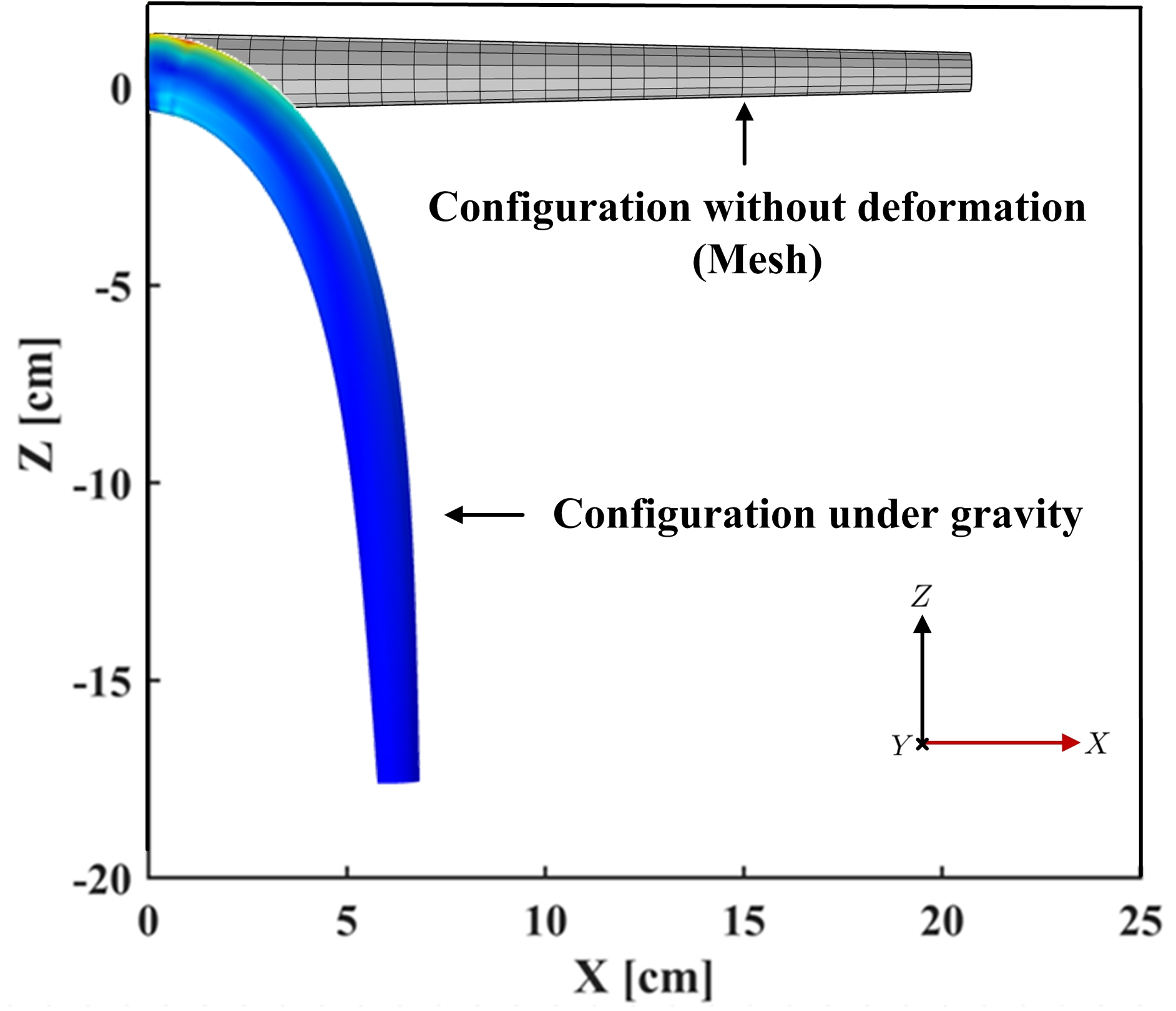
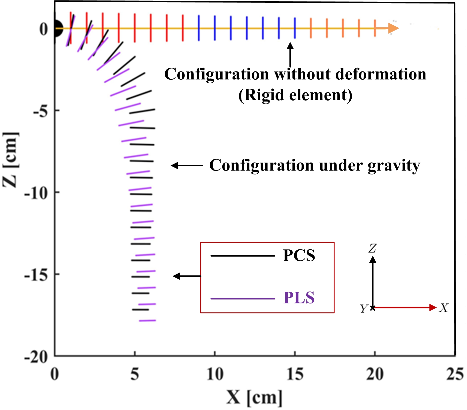
Refer to caption
(a)
Refer to caption
(b)
Figure 5: Simulation comparison of three different modeling methods for the cantilever rod before and after deformation. (a) FEM. (b) PCS and PLS Cosserat models in MATLAB.
TABLE II: Comparison results of PCS and PLS Cosserat static models w.r.t. FEM under gravity in terms of end-effector position and its relative error
Modeling method
Position of end-effector
(Unit:cmcm\rm{cm})
Relative error of end-
effector position w.r.t.
FEM (Unit: %percent\%)
uxsubscript𝑢𝑥u_{x} uysubscript𝑢𝑦u_{y} uzsubscript𝑢𝑧u_{z} exsubscript𝑒𝑥e_{x} eysubscript𝑒𝑦e_{y} ezsubscript𝑒𝑧e_{z}
FEM 5.8479 0.0000 -17.8395 ×\times ×\times ×\times
PCS [23] 5.3450 0.0000 -17.1693 -8.60 0.00 -16.88
PLS 5.7787 0.0000 -17.8394 -1.18 0.00 -0.01

V-C Accuracy Comparison of PLS Model with Different Modes

Based on the aforementioned manipulator parameters setting, different models via the PLS Cosserat involving Euler-Bernoulli (E-B), extensible Kirchhoff (E-K) and Timoshenko beams are established by strain mode selection. These beams are fixed at X=0𝑋0X=0, and subject to gravity as well as an external imposed concentrated load with 𝓕tip=[0,0,0,F,0,0]Tsubscript𝓕tipsuperscript000𝐹00T\small\boldsymbol{\mathcal{F}}_{\rm{tip}}=[0,0,0,F,0,0]^{\rm T} (i.e., tension along X𝑋X-axis) at X=L𝑋𝐿X=L. The three-dimensional static simulation is implemented by increasing load with increment of 0.05N0.05N0.05\ {\rm N} at a time. Fig. 6(LABEL:sub@E-C-LABEL:sub@C_E-K) displays a contrast of the evolution of the equilibrium configurations among these beams for several sets of the tip load, and Table III shows different beams’ end-effector positions versus that of FEM. The results indicate that it is feasible to remove negligible modes in some particular case with low-precision requirement, which contributes to the real-time simulation and control.

TABLE III: Comparison results of different beam models via PLS Cosserat w.r.t. FEM under gravity in terms of end-effector position and its relative error
Modeling method
Position of end-effector
(Unit:cmcm\rm{cm})
Relative error of end-
effector position w.r.t.
FEM (Unit: %percent\%)
uxsubscript𝑢𝑥u_{x} uysubscript𝑢𝑦u_{y} uzsubscript𝑢𝑧u_{z} exsubscript𝑒𝑥e_{x} eysubscript𝑒𝑦e_{y} ezsubscript𝑒𝑧e_{z}
FEM 5.8479 0.0000 -17.8395 - - -
Cosserat 5.7787 0.0000 -17.8394 -1.18 0.00 -0.01
E-B 5.4940 0.0000 -17.7527 -6.05 0.00 -0.49
E-K 5.6925 0.0000 -17.8523 -2.66 0.00 0.07
Timoshenko 5.3596 0.0000 -17.9002 -8.35 0.00 0.34
Refer to caption
(a)
Refer to caption
(b)
Refer to caption
(c)
Figure 6: Deformation comparison among beam models via PLS Cosserat under external loads. (a) Cosserat versus Euler-Bernoulli. (b) Cosserat versus Timoshenko. (c) Cosserat versus extensible Kirchhoff.

VI PLS Cosserat model validation

VI-A Studied Soft Manipulator

A prototype of soft manipulator, similar to that used in the simulation, was designed to carry out the material parameters identification of the PLS Cosserat model by the real input-output relationship obtained from the experimental setup. The exact geometric parameters of the manipulator are illustrated in Fig. 7. The investigated soft arm is controlled by 4 cables mounted through it from the base to the tip, and the cables are respectively driven by different weights, as shown in Fig. 8. Aiming at obtaining the position of the end-effector, a magnetic sensor is positioned on the tip of the arm, and for this purpose, a long and conical hole was made along the whole length of the arm. In addition, several 3D-printed rigid rings are mounted along the soft manipulator to minimize friction between the cables and a single conical piece of silicone. Finally, the casting material of the manipulator is an isotropic silicone rubber.
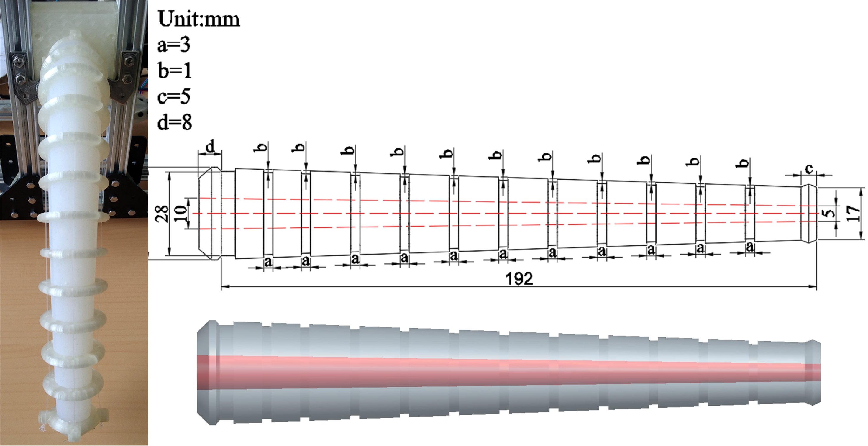
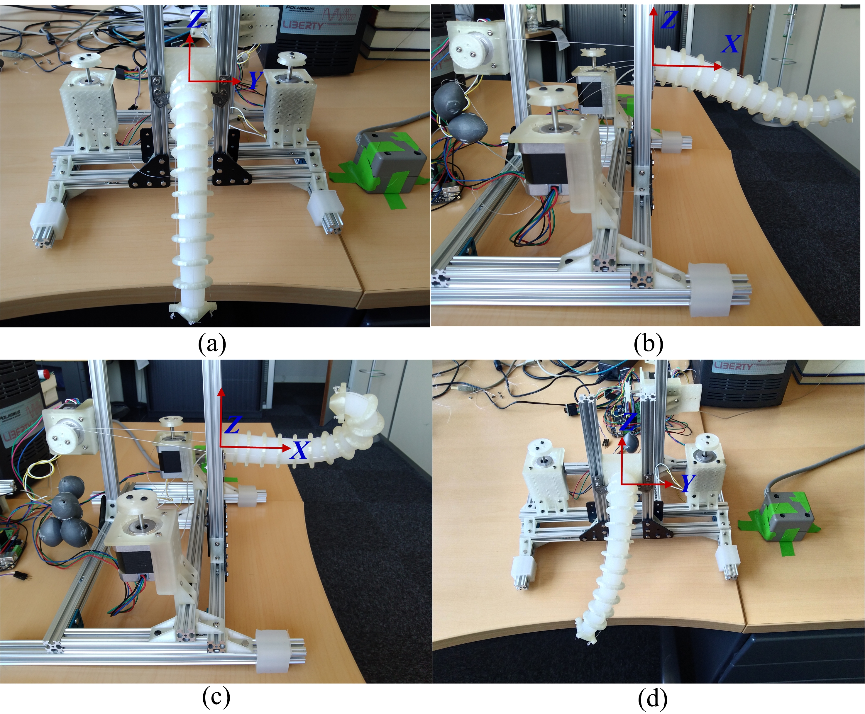
Refer to caption
Figure 7: Manipulator prototype design.
Refer to caption
Figure 8: Several snapshots of the different experiments for implementing parameters identification.
TABLE IV: Experimental samples for identification algorithm
Order of Cables’ tension 𝑻isubscript𝑻𝑖\boldsymbol{T}_{i} Position of the
experiment (Unit: N) end-effector 𝒖eisubscript𝒖𝑒𝑖\boldsymbol{u}_{ei} (Unit: cmcm\rm{cm})
1 [0000]delimited-[]matrix0000[\begin{matrix}0&0&0&0\end{matrix}] [15.770.0310.10]delimited-[]matrix15.770.0310.10[\begin{matrix}15.77&0.03&-10.10\end{matrix}]
2 [0000.98]delimited-[]matrix0000.98[\begin{matrix}0&0&0&0.98\end{matrix}] [17.730.026.44]delimited-[]matrix17.730.026.44[\begin{matrix}17.73&0.02&-6.44\end{matrix}]
3 [0.98004.90]delimited-[]matrix0.98004.90[\begin{matrix}0.98&0&0&4.90\end{matrix}] [6.854.777.20]delimited-[]matrix6.854.777.20[\begin{matrix}6.85&-4.77&7.20\end{matrix}]
4 [0001.96]delimited-[]matrix0001.96[\begin{matrix}0&0&0&1.96\end{matrix}] [18.310.011.90]delimited-[]matrix18.310.011.90[\begin{matrix}18.31&0.01&-1.90\end{matrix}]
5 [1.96001.96]delimited-[]matrix1.96001.96[\begin{matrix}1.96&0&0&1.96\end{matrix}] [13.099.242.46]delimited-[]matrix13.099.242.46[\begin{matrix}13.09&-9.24&-2.46\end{matrix}]
6 [0.98000]delimited-[]matrix0.98000[\begin{matrix}0.98&0&0&0\end{matrix}] [14.724.209.78]delimited-[]matrix14.724.209.78[\begin{matrix}14.72&-4.20&-9.78\end{matrix}]

VI-B Validation and Discussion

The model validation which determines whether the model is proper enough for its intended use is implemented. Six sets of experiments are performed to acquire the position information of end-effector under the effect of different loads exerted by weights equivalent to the cable’s tension. Table IV provides specific input and output values of the experiments, and the position as well as orientation of the manipulator in several cases are displayed in Fig. 8. Subsequently, the experimental outputs obtained by the position sensor are utilized to realize the proposed parameters identification algorithm, and thus the material parameters 𝜽𝜽\small\boldsymbol{\theta} can be calculated.

The material parameters obtained by solving the NLP problem are as follows: Young’s modulus E=2.563×10⁵Pa𝐸2.563superscript105PaE=2.563\times 10^{5}\ {\rm{Pa}}, shear modulus G=8.543×10⁴Pa𝐺8.543superscript104PaG=8.543\times 10^{4}\ {\rm{Pa}}, and density of material ρ=1.41×10³kg/m3𝜌1.41superscript103kgsuperscriptm3\rho=1.41\times 10^{3}\ {\rm{kg/m^{3}}}.

After that, model validation is performed to verify the accuracy of the PLS Cosserat model with the identified parameters. Considering uncertain factors of the experiment, we repeat 10 times for each input and then obtain the average of end-effector position to compare with simulation, five different groups of control inputs and average of outputs provided in Table V are selected to compare the position and orientation of the soft arm between the experiments and simulations. The comparison results indicate the outputs (position of the end-effector) from the PLS Cosserat model are almost identical to those of the experiments in three cases illustrated in Fig. 9. As for the remaining two sets of experiments, there are larger absolute errors of end-effector position between the model and manipulator than those from the other three cases, which may be due to tiny pleats on the silicone surface caused by relatively larger cables’ tension.
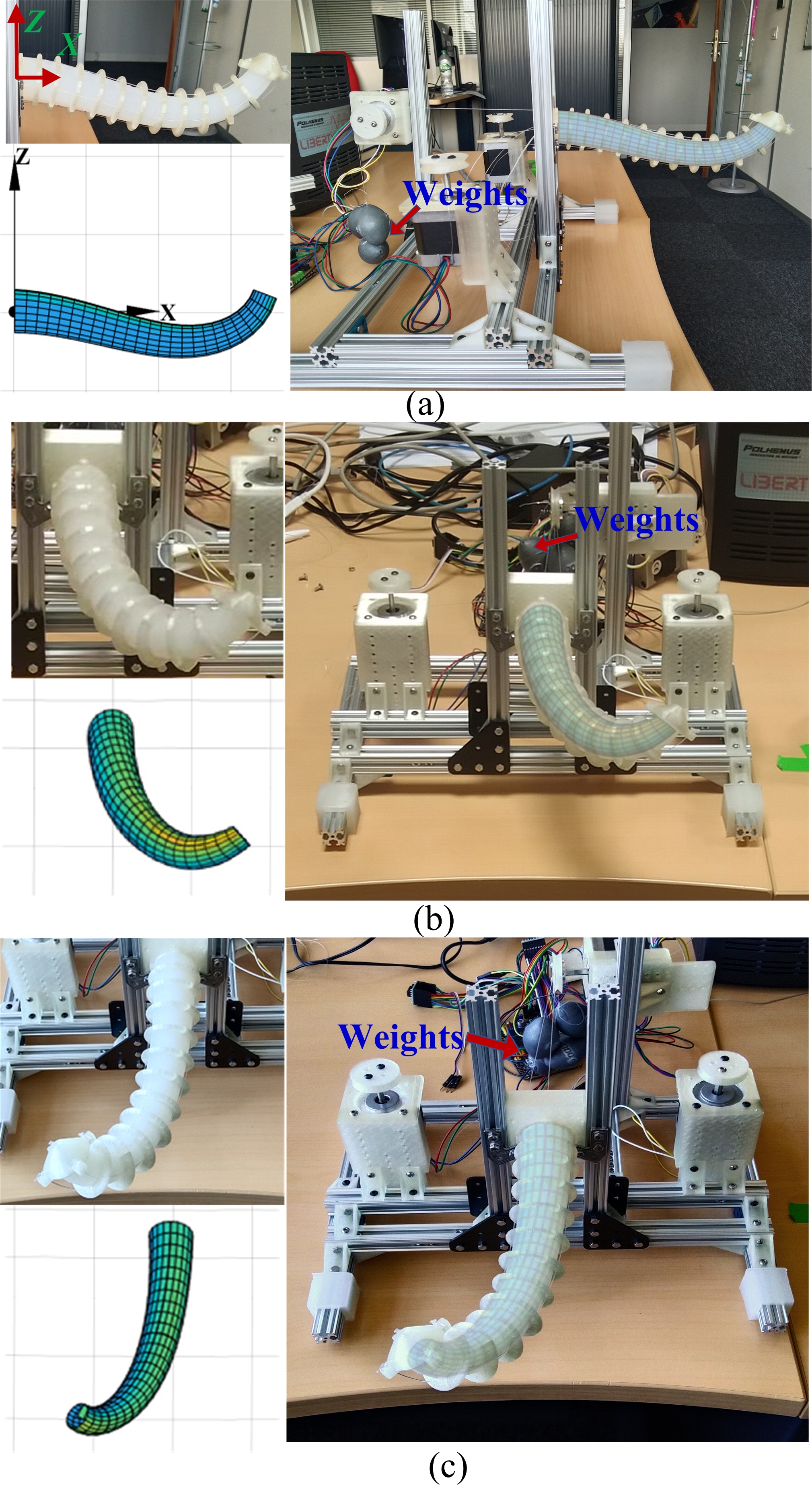
Refer to caption
Figure 9: Configuration comparison between simulation and experiment under gravity and different cables’ tension. (a) 𝑻=[0002.94]T𝑻superscriptdelimited-[]matrix0002.94T\boldsymbol{T}=\left[\begin{matrix}0&0&0&2.94\end{matrix}\right]^{\rm T}. (b) 𝑻=[001.961.96]T𝑻superscriptdelimited-[]matrix001.961.96T\boldsymbol{T}=\left[\begin{matrix}0&0&1.96&1.96\end{matrix}\right]^{\rm T}. (c) 𝑻=[0.98002.94]T𝑻superscriptdelimited-[]matrix0.98002.94T\boldsymbol{T}=\left[\begin{matrix}0.98&0&0&2.94\end{matrix}\right]^{\rm T}.
TABLE V: Different experiments for model validation
Order of Cables’ tension 𝑻isubscript𝑻𝑖\boldsymbol{T}_{i} Average of position of end-
control input (Unit: N) effector 𝒖eisubscript𝒖𝑒𝑖\small\boldsymbol{u}_{ei} (Unit: cmcm{\rm{cm}})
1 (10 times) [0002.94]delimited-[]matrix0002.94[\begin{matrix}0&0&0&2.94\end{matrix}] [16.810.032.87]delimited-[]matrix16.810.032.87[\begin{matrix}16.81&0.03&2.87\end{matrix}]
2 (10 times) [001.961.96]delimited-[]matrix001.961.96[\begin{matrix}0&0&1.96&1.96\end{matrix}] [13.229.422.37]delimited-[]matrix13.229.422.37[\begin{matrix}13.22&9.42&-2.37\end{matrix}]
3 (10 times) [0.98002.94]delimited-[]matrix0.98002.94[\begin{matrix}0.98&0&0&2.94\end{matrix}] [14.976.032.53]delimited-[]matrix14.976.032.53[\begin{matrix}14.97&-6.03&2.53\end{matrix}]
4 (10 times) [002.946.86]delimited-[]matrix002.946.86[\begin{matrix}0&0&2.94&6.86\end{matrix}] [1.503.692.26]delimited-[]matrix1.503.692.26[\begin{matrix}1.50&3.69&2.26\end{matrix}]
5 (10 times) [0005.88]delimited-[]matrix0005.88[\begin{matrix}0&0&0&5.88\end{matrix}] [4.280.027.55]delimited-[]matrix4.280.027.55[\begin{matrix}4.28&0.02&7.55\end{matrix}]
Refer to caption
Figure 10: The illustration of absolute errors of the end-effector position for the PLS Cosserat model and soft manipulator under different control inputs.

The absolute errors of the end-effector position of the model with respect to those of the experiments are all less than 5mm5mm5\ {\rm{mm}}, as shown in Fig. 10, further showing the effectiveness of this parameters identification method and the accuracy of the PLS Cosserat model.

VII Conclusion and future work

A piecewise linear strain Cosserat dynamics model for the soft manipulator has been developed for the first time, which combines the advantages of the PCS and VS Cosserat models. This method depends on a rigorous mathematical framework via the Lie group theory which facilitates a natural coupling of the position and the orientation variables, and exhibits an important advantage over avoiding the difficulty in the parameterization of rotation matrix. The PLS Cosserat model has been compared with the discrete models reported in the published literature, showing comparable to the FEM and even better results than the PCS Cosserat model in terms of accuracy. As proved in the section V, the PLS Cosserat model shows great potential to be universally applied to the modeling of slender rod-like soft arms in a real scenario.

The parameters identification based on the PLS Cosserat static model can be considered as a NLP problem with several nonlinear equality constraints. A general framework has been proposed for the material parameters estimation, which is applicable to identify the parameters of the soft manipulators with arbitrary actuation manner. To carry out the model validation, we designed a manipulator prototype made of silicone and established the experimental platform. Both simulation and experiment results indicate the proposed scheme is able to identify the material parameters of soft arm with higher precision, and provides the possibility for developing the model-based controller..

The standard Lagrangian formulation in (31) for PLS Cosserat dynamic model will be used to design static and dynamic model-based controllers due to the relative parameterization of the soft arm actuated by cables in the near future.

Acknowledgments

This work is partially supported by project COSSEROOTS. The author Haihong Li gratefully acknowledge the support from the China Scholarship Council (Grant no. 202008440356).

[]

-A Analytic solution of differential kinematics model

Based on the aforementioned two assumptions, the rightmost velocity of any segment j𝑗j along the section n𝑛n at time t𝑡t can be calculated by means of the integral of DE (2).

𝜼(Ln1+jΔX)=[i=0j1eΔXad𝝃n(Ln1+iΔX)]𝜼(Ln1)+i=1j{[τ=ij1eΔXad𝝃n(Ln1+τΔX)]Ln1+(i1)ΔXLn1+iΔXe(sLn1iΔX)ad𝝃n(Ln1+(i1)ΔX)𝝃˙n(Ln1+(i1)ΔX)ds}𝜼subscript𝐿𝑛1𝑗Δ𝑋delimited-[]superscriptsubscriptproduct𝑖0𝑗1superscript𝑒Δ𝑋subscriptadsubscript𝝃𝑛subscript𝐿𝑛1𝑖Δ𝑋𝜼subscript𝐿𝑛1superscriptsubscript𝑖1𝑗delimited-[]superscriptsubscriptproduct𝜏𝑖𝑗1superscript𝑒Δ𝑋subscriptadsubscript𝝃𝑛subscript𝐿𝑛1𝜏Δ𝑋superscriptsubscriptsubscript𝐿𝑛1𝑖1Δ𝑋subscript𝐿𝑛1𝑖Δ𝑋superscript𝑒𝑠subscript𝐿𝑛1𝑖Δ𝑋subscriptadsubscript𝝃𝑛subscript𝐿𝑛1𝑖1Δ𝑋subscript˙𝝃𝑛subscript𝐿𝑛1𝑖1Δ𝑋d𝑠\displaystyle\scriptsize\begin{split}&\boldsymbol{\eta}(L_{n-1}+j\Delta X)=\left[\prod_{i=0}^{j-1}e^{-\Delta X{\rm ad}_{\boldsymbol{\xi}_{n}(L_{n-1}+i\Delta X)}}\right]\boldsymbol{\eta}(L_{n-1})+\\ &\sum_{i=1}^{j}\Biggl{\{}\Bigg{[}\prod_{\tau=i}^{j-1}e^{-\Delta X{\rm ad}_{\boldsymbol{\xi}_{n}(L_{n-1}+\tau\Delta X)}}\Bigg{]}\int_{L_{n-1}+(i-1)\Delta X}^{L_{n-1}+i\Delta X}\\ &e^{(s-L_{n-1}-i\Delta X){\rm ad}_{\boldsymbol{\xi}_{n}(L_{n-1}+(i-1)\Delta X)}}\dot{\boldsymbol{\xi}}_{n}\Big{(}L_{n-1}+(i-1)\Delta X\Big{)}{\rm d}s\Biggr{\}}\end{split}

After that, the velocity of each cross section along the section n𝑛n at time t𝑡t can be analytically obtained

𝜼(X)=e(XLn1jΔX)ad𝝃n(Ln1+jΔX){[i=0j1eΔXad𝝃n(Ln1+iΔX)]𝜼(Ln1)+i=1j[(τ=ij1eΔXad𝝃n(Ln1+τΔX))Ln1+(i1)ΔXLn1+iΔXe(sLn1iΔX)ad𝝃n(Ln1+(i1)ΔX)𝝃˙n(Ln1+(i1)ΔX)ds]}+Ln1+jΔXXe(Xs)ad𝝃n(Ln1+jΔX)𝝃˙n(Ln1+jΔX)ds𝜼𝑋superscript𝑒𝑋subscript𝐿𝑛1𝑗Δ𝑋subscriptadsubscript𝝃𝑛subscript𝐿𝑛1𝑗Δ𝑋delimited-[]superscriptsubscriptproduct𝑖0𝑗1superscript𝑒Δ𝑋subscriptadsubscript𝝃𝑛subscript𝐿𝑛1𝑖Δ𝑋𝜼subscript𝐿𝑛1superscriptsubscript𝑖1𝑗delimited-[]superscriptsubscriptproduct𝜏𝑖𝑗1superscript𝑒Δ𝑋subscriptadsubscript𝝃𝑛subscript𝐿𝑛1𝜏Δ𝑋superscriptsubscriptsubscript𝐿𝑛1𝑖1Δ𝑋subscript𝐿𝑛1𝑖Δ𝑋superscript𝑒𝑠subscript𝐿𝑛1𝑖Δ𝑋subscriptadsubscript𝝃𝑛subscript𝐿𝑛1𝑖1Δ𝑋subscript˙𝝃𝑛subscript𝐿𝑛1𝑖1Δ𝑋d𝑠superscriptsubscriptsubscript𝐿𝑛1𝑗Δ𝑋𝑋superscript𝑒𝑋𝑠subscriptadsubscript𝝃𝑛subscript𝐿𝑛1𝑗Δ𝑋subscript˙𝝃𝑛subscript𝐿𝑛1𝑗Δ𝑋differential-d𝑠\scriptsize\begin{split}&\boldsymbol{\eta}(X)=e^{-(X-L_{n-1}-j\Delta X){\rm{ad}}_{\boldsymbol{\xi}_{n}(L_{n-1}+j\Delta X)}}\\ &\Biggl{\{}\Big{[}\prod_{i=0}^{j-1}e^{-\Delta X{\rm ad}_{\boldsymbol{\xi}_{n}(L_{n-1}+i\Delta X)}}\Big{]}\boldsymbol{\eta}(L_{n-1})\\ &\quad+\sum_{i=1}^{j}\Big{[}\Big{(}\prod_{\tau=i}^{j-1}e^{-\Delta X{\rm ad}_{\boldsymbol{\xi}_{n}(L_{n-1}+\tau\Delta X)}}\Big{)}\int_{L_{n-1}+(i-1)\Delta X}^{L_{n-1}+i\Delta X}\\ &\quad e^{(s-L_{n-1}-i\Delta X){\rm ad}_{\boldsymbol{\xi}_{n}(L_{n-1}+(i-1)\Delta X)}}\dot{\boldsymbol{\xi}}_{n}\Big{(}L_{n-1}+(i-1)\Delta X\Big{)}{\rm d}s\Big{]}\Biggr{\}}\\ &\quad+\int_{L_{n-1}+j\Delta X}^{X}e^{-(X-s){\rm{ad}}_{\boldsymbol{\xi}_{n}(L_{n-1}+j\Delta X)}}\dot{{\boldsymbol{\xi}}}_{n}\Big{(}L_{n-1}+j\Delta X\Big{)}{\rm d}s\end{split}

Under the PLS assumption, the velocity of any cross section at X𝑋X and along the section n𝑛n at time t𝑡t can be re-formulated as follows

𝜼(X)=e(XLn1jΔX)adΘnj{(i=0j1eadΔXΘni)𝜼(Ln1)+i=1j[(τ=ij1eadΔXΘnτ)Ln1+(i1)ΔXLn1+iΔXe(sLn1iΔX)adΘn(i1)αn(i1)ds]𝝃¯˙n1+i=1j[(τ=ij1eadΔXΘnτ)Ln1+(i1)ΔXLn1+iΔXe(sLn1iΔX)adΘn(i1)βn(i1)ds]𝝃¯˙n}+Ln1+jΔXXe(Xs)adΘnjαnjds𝝃¯˙n1+Ln1+jΔXXe(Xs)adΘnjβnjds𝝃¯˙n𝜼𝑋superscript𝑒𝑋subscript𝐿𝑛1𝑗Δ𝑋subscriptadsuperscriptsubscriptΘ𝑛𝑗superscriptsubscriptproduct𝑖0𝑗1superscript𝑒subscriptadΔ𝑋superscriptsubscriptΘ𝑛𝑖𝜼subscript𝐿𝑛1superscriptsubscript𝑖1𝑗delimited-[]superscriptsubscriptproduct𝜏𝑖𝑗1superscript𝑒subscriptadΔ𝑋superscriptsubscriptΘ𝑛𝜏superscriptsubscriptsubscript𝐿𝑛1𝑖1Δ𝑋subscript𝐿𝑛1𝑖Δ𝑋superscript𝑒𝑠subscript𝐿𝑛1𝑖Δ𝑋subscriptadsuperscriptsubscriptΘ𝑛𝑖1subscript𝛼𝑛𝑖1d𝑠subscript˙¯𝝃𝑛1superscriptsubscript𝑖1𝑗delimited-[]superscriptsubscriptproduct𝜏𝑖𝑗1superscript𝑒subscriptadΔ𝑋superscriptsubscriptΘ𝑛𝜏superscriptsubscriptsubscript𝐿𝑛1𝑖1Δ𝑋subscript𝐿𝑛1𝑖Δ𝑋superscript𝑒𝑠subscript𝐿𝑛1𝑖Δ𝑋subscriptadsuperscriptsubscriptΘ𝑛𝑖1subscript𝛽𝑛𝑖1d𝑠subscript˙¯𝝃𝑛superscriptsubscriptsubscript𝐿𝑛1𝑗Δ𝑋𝑋superscript𝑒𝑋𝑠subscriptadsuperscriptsubscriptΘ𝑛𝑗subscript𝛼𝑛𝑗differential-d𝑠subscript˙¯𝝃𝑛1superscriptsubscriptsubscript𝐿𝑛1𝑗Δ𝑋𝑋superscript𝑒𝑋𝑠subscriptadsuperscriptsubscriptΘ𝑛𝑗subscript𝛽𝑛𝑗differential-d𝑠subscript˙¯𝝃𝑛\scriptsize\begin{split}\boldsymbol{\eta}(X)&=e^{-(X-L_{n-1}-j\Delta X){\rm{ad}}_{\Theta_{nj}^{\vee}}}\Biggl{\{}\Big{(}\prod_{i=0}^{j-1}e^{-{\rm ad}_{\Delta X\Theta_{ni}^{\vee}}}\Big{)}\boldsymbol{\eta}(L_{n-1})\\ &\quad+\sum_{i=1}^{j}\Big{[}\Big{(}\prod_{\tau=i}^{j-1}e^{-{\rm ad}_{\Delta X\Theta_{n\tau}^{\vee}}}\Big{)}\int_{L_{n-1}+(i-1)\Delta X}^{L_{n-1}+i\Delta X}\\ &\qquad e^{(s-L_{n-1}-i\Delta X){\rm ad}_{\Theta_{n(i-1)}^{\vee}}}\alpha_{n(i-1)}{\rm d}s\Big{]}\dot{\overline{\boldsymbol{\xi}}}_{n-1}\\ &\quad+\sum_{i=1}^{j}\Big{[}\Big{(}\prod_{\tau=i}^{j-1}e^{-{\rm ad}_{\Delta X\Theta_{n\tau}^{\vee}}}\Big{)}\int_{L_{n-1}+(i-1)\Delta X}^{L_{n-1}+i\Delta X}\\ &\qquad e^{(s-L_{n-1}-i\Delta X){\rm ad}_{\Theta_{n(i-1)}^{\vee}}}\beta_{n(i-1)}{\rm d}s\Big{]}\dot{\overline{\boldsymbol{\xi}}}_{n}\Biggr{\}}\\ &\quad+\int_{L_{n-1}+j\Delta X}^{X}e^{-(X-s){\rm{ad}}_{\Theta_{nj}^{\vee}}}\alpha_{nj}{\rm d}s\dot{\overline{\boldsymbol{\xi}}}_{n-1}\\ &\quad+\int_{L_{n-1}+j\Delta X}^{X}e^{-(X-s){\rm{ad}}_{\Theta_{nj}^{\vee}}}\beta_{nj}{\rm d}s\dot{\overline{\boldsymbol{\xi}}}_{n}\end{split} (32)

with Θni=αni𝝃¯^n1+βni𝝃¯^nsubscriptΘ𝑛𝑖subscript𝛼𝑛𝑖subscript^¯𝝃𝑛1subscript𝛽𝑛𝑖subscript^¯𝝃𝑛\scriptsize\Theta_{ni}=\alpha_{ni}\widehat{\overline{\boldsymbol{\xi}}}_{n-1}+\beta_{ni}\widehat{\overline{\boldsymbol{\xi}}}_{n}, Θnj=αnj𝝃¯^n1+βnj𝝃¯^nsubscriptΘ𝑛𝑗subscript𝛼𝑛𝑗subscript^¯𝝃𝑛1subscript𝛽𝑛𝑗subscript^¯𝝃𝑛\scriptsize\Theta_{nj}=\alpha_{nj}\widehat{\overline{\boldsymbol{\xi}}}_{n-1}+\beta_{nj}\widehat{\overline{\boldsymbol{\xi}}}_{n}, where αni=1iΔXLnLn1subscript𝛼𝑛𝑖1𝑖Δ𝑋subscript𝐿𝑛subscript𝐿𝑛1\alpha_{ni}=1-\frac{i\Delta X}{L_{n}-L_{n-1}}, βni=iΔXLnLn1subscript𝛽𝑛𝑖𝑖Δ𝑋subscript𝐿𝑛subscript𝐿𝑛1\beta_{ni}=\frac{i\Delta X}{L_{n}-L_{n-1}}, αnj=1jΔXLnLn1subscript𝛼𝑛𝑗1𝑗Δ𝑋subscript𝐿𝑛subscript𝐿𝑛1\alpha_{nj}=1-\frac{j\Delta X}{L_{n}-L_{n-1}}, βnj=jΔXLnLn1subscript𝛽𝑛𝑗𝑗Δ𝑋subscript𝐿𝑛subscript𝐿𝑛1\beta_{nj}=\frac{j\Delta X}{L_{n}-L_{n-1}}.

By the same reasoning, the rightmost acceleration of any segment j𝑗j of the section n𝑛n along the soft manipulator can be computed at time t𝑡t by the use of the integral of (3).

𝜼˙(Ln1+jΔX)=[i=0j1eΔXad𝝃n(Ln1+iΔX)]𝜼˙(Ln1)+i=1j{[τ=ij1eΔXad𝝃n(Ln1+τΔX)]Ln1+(i1)ΔXLn1+iΔXe(sLn1iΔX)ad𝝃n(Ln1+(i1)ΔX)ds𝝃¨n(Ln1+(i1)ΔX)}+i=1j{[τ=ij1eΔXad𝝃n(Ln1+τΔX)]Ln1+(i1)ΔXLn1+iΔXe(sLn1iΔX)ad𝝃n(Ln1+(i1)ΔX)ad𝜼(s)ds𝝃˙n(Ln1+(i1)ΔX)}˙𝜼subscript𝐿𝑛1𝑗Δ𝑋delimited-[]superscriptsubscriptproduct𝑖0𝑗1superscript𝑒Δ𝑋subscriptadsubscript𝝃𝑛subscript𝐿𝑛1𝑖Δ𝑋˙𝜼subscript𝐿𝑛1superscriptsubscript𝑖1𝑗delimited-[]superscriptsubscriptproduct𝜏𝑖𝑗1superscript𝑒Δ𝑋subscriptadsubscript𝝃𝑛subscript𝐿𝑛1𝜏Δ𝑋superscriptsubscriptsubscript𝐿𝑛1𝑖1Δ𝑋subscript𝐿𝑛1𝑖Δ𝑋superscript𝑒𝑠subscript𝐿𝑛1𝑖Δ𝑋subscriptadsubscript𝝃𝑛subscript𝐿𝑛1𝑖1Δ𝑋d𝑠subscript¨𝝃𝑛subscript𝐿𝑛1𝑖1Δ𝑋superscriptsubscript𝑖1𝑗delimited-[]superscriptsubscriptproduct𝜏𝑖𝑗1superscript𝑒Δ𝑋subscriptadsubscript𝝃𝑛subscript𝐿𝑛1𝜏Δ𝑋superscriptsubscriptsubscript𝐿𝑛1𝑖1Δ𝑋subscript𝐿𝑛1𝑖Δ𝑋superscript𝑒𝑠subscript𝐿𝑛1𝑖Δ𝑋subscriptadsubscript𝝃𝑛subscript𝐿𝑛1𝑖1Δ𝑋subscriptad𝜼sd𝑠subscript˙𝝃𝑛subscript𝐿𝑛1𝑖1Δ𝑋\scriptsize\begin{split}&\dot{\boldsymbol{\eta}}(L_{n-1}+j\Delta X)=\left[\prod_{i=0}^{j-1}e^{-\Delta X{\rm ad}_{\boldsymbol{\xi}_{n}(L_{n-1}+i\Delta X)}}\right]\dot{\boldsymbol{\eta}}(L_{n-1})\\ &+\sum_{i=1}^{j}\Biggl{\{}\left[\prod_{\tau=i}^{j-1}e^{-\Delta X{\rm ad}_{\boldsymbol{\xi}_{n}(L_{n-1}+\tau\Delta X)}}\right]\int_{L_{n-1}+(i-1)\Delta X}^{L_{n-1}+i\Delta X}\\ &e^{(s-L_{n-1}-i\Delta X){\rm ad}_{\boldsymbol{\xi}_{n}(L_{n-1}+(i-1)\Delta X)}}{\rm d}s\ddot{\boldsymbol{\xi}}_{n}\Big{(}L_{n-1}+(i-1)\Delta X\Big{)}\Biggr{\}}\\ &+\sum_{i=1}^{j}\Biggl{\{}\left[\prod_{\tau=i}^{j-1}e^{-\Delta X{\rm ad}_{\boldsymbol{\xi}_{n}(L_{n-1}+\tau\Delta X)}}\right]\int_{L_{n-1}+(i-1)\Delta X}^{L_{n-1}+i\Delta X}\\ &e^{(s-L_{n-1}-i\Delta X){\rm ad}_{\boldsymbol{\xi}_{n}(L_{n-1}+(i-1)\Delta X)}}{\rm{ad}_{\boldsymbol{\eta}(s)}}{\rm d}s\dot{\boldsymbol{\xi}}_{n}\Big{(}L_{n-1}+(i-1)\Delta X\Big{)}\Biggr{\}}\end{split}

Considering the PLS hypothesis, the acceleration of any cross section at X𝑋X and along the section n𝑛n at time t𝑡t can be re-written as follows

𝜼˙(X)=e(XLn1jΔX)adΘnj{(i=0j1eadΔXΘni)𝜼˙(Ln1)+i=1j[(τ=ij1eadΔXΘnτ)Ln1+(i1)ΔXLn1+iΔXe(sLn1iΔX)adΘn(i1)αn(i1)ds]𝝃¯¨n1+i=1j[(τ=ij1eadΔXΘnτ)Ln1+(i1)ΔXLn1+iΔXe(sLn1iΔX)adΘn(i1)βn(i1)ds]𝝃¯¨n+i=1j[(τ=ij1eadΔXΘnτ)Ln1+(i1)ΔXLn1+iΔXe(sLn1iΔX)adΘn(i1)ad𝜼(s)αn(i1)ds]𝝃¯˙n1+i=1j[(τ=ij1eadΔXΘnτ)Ln1+(i1)ΔXLn1+iΔXe(sLn1iΔX)adΘn(i1)ad𝜼(s)βn(i1)ds]𝝃¯˙n}+Ln1+jΔXXe(Xs)adΘnjαnjds𝝃¯¨n1+Ln1+jΔXXe(Xs)adΘnjβnjds𝝃¯¨n+Ln1+jΔXXe(Xs)adΘnjad𝜼(s)αnjds𝝃¯˙n1+Ln1+jΔXXe(Xs)adΘnjad𝜼(s)βnjds𝝃¯˙n˙𝜼𝑋superscript𝑒𝑋subscript𝐿𝑛1𝑗Δ𝑋subscriptadsuperscriptsubscriptΘ𝑛𝑗superscriptsubscriptproduct𝑖0𝑗1superscript𝑒subscriptadΔ𝑋superscriptsubscriptΘ𝑛𝑖˙𝜼subscript𝐿𝑛1superscriptsubscript𝑖1𝑗delimited-[]superscriptsubscriptproduct𝜏𝑖𝑗1superscript𝑒subscriptadΔ𝑋superscriptsubscriptΘ𝑛𝜏superscriptsubscriptsubscript𝐿𝑛1𝑖1Δ𝑋subscript𝐿𝑛1𝑖Δ𝑋superscript𝑒𝑠subscript𝐿𝑛1𝑖Δ𝑋subscriptadsuperscriptsubscriptΘ𝑛𝑖1subscript𝛼𝑛𝑖1d𝑠subscript¨¯𝝃𝑛1superscriptsubscript𝑖1𝑗delimited-[]superscriptsubscriptproduct𝜏𝑖𝑗1superscript𝑒subscriptadΔ𝑋superscriptsubscriptΘ𝑛𝜏superscriptsubscriptsubscript𝐿𝑛1𝑖1Δ𝑋subscript𝐿𝑛1𝑖Δ𝑋superscript𝑒𝑠subscript𝐿𝑛1𝑖Δ𝑋subscriptadsuperscriptsubscriptΘ𝑛𝑖1subscript𝛽𝑛𝑖1d𝑠subscript¨¯𝝃𝑛superscriptsubscript𝑖1𝑗delimited-[]superscriptsubscriptproduct𝜏𝑖𝑗1superscript𝑒subscriptadΔ𝑋superscriptsubscriptΘ𝑛𝜏superscriptsubscriptsubscript𝐿𝑛1𝑖1Δ𝑋subscript𝐿𝑛1𝑖Δ𝑋superscript𝑒𝑠subscript𝐿𝑛1𝑖Δ𝑋subscriptadsuperscriptsubscriptΘ𝑛𝑖1subscriptad𝜼𝑠subscript𝛼𝑛𝑖1d𝑠subscript˙¯𝝃𝑛1superscriptsubscript𝑖1𝑗delimited-[]superscriptsubscriptproduct𝜏𝑖𝑗1superscript𝑒subscriptadΔ𝑋superscriptsubscriptΘ𝑛𝜏superscriptsubscriptsubscript𝐿𝑛1𝑖1Δ𝑋subscript𝐿𝑛1𝑖Δ𝑋superscript𝑒𝑠subscript𝐿𝑛1𝑖Δ𝑋subscriptadsuperscriptsubscriptΘ𝑛𝑖1subscriptad𝜼ssubscript𝛽𝑛𝑖1d𝑠subscript˙¯𝝃𝑛superscriptsubscriptsubscript𝐿𝑛1𝑗Δ𝑋𝑋superscript𝑒𝑋𝑠subscriptadsuperscriptsubscriptΘ𝑛𝑗subscript𝛼𝑛𝑗differential-d𝑠subscript¨¯𝝃𝑛1superscriptsubscriptsubscript𝐿𝑛1𝑗Δ𝑋𝑋superscript𝑒𝑋𝑠subscriptadsuperscriptsubscriptΘ𝑛𝑗subscript𝛽𝑛𝑗differential-d𝑠subscript¨¯𝝃𝑛superscriptsubscriptsubscript𝐿𝑛1𝑗Δ𝑋𝑋superscript𝑒𝑋𝑠subscriptadsuperscriptsubscriptΘ𝑛𝑗subscriptad𝜼𝑠subscript𝛼𝑛𝑗differential-d𝑠subscript˙¯𝝃𝑛1superscriptsubscriptsubscript𝐿𝑛1𝑗Δ𝑋𝑋superscript𝑒𝑋𝑠subscriptadsuperscriptsubscriptΘ𝑛𝑗subscriptad𝜼𝑠subscript𝛽𝑛𝑗differential-d𝑠subscript˙¯𝝃𝑛\scriptsize\begin{split}\dot{\boldsymbol{\eta}}(X)&=e^{-(X-L_{n-1}-j\Delta X){\rm{ad}}_{\Theta_{nj}^{\vee}}}\Biggl{\{}\Big{(}\prod_{i=0}^{j-1}e^{-{\rm ad}_{\Delta X\Theta_{ni}^{\vee}}}\Big{)}\dot{\boldsymbol{\eta}}(L_{n-1})\\ &+\sum_{i=1}^{j}\Big{[}\Big{(}\prod_{\tau=i}^{j-1}e^{-{\rm ad}_{\Delta X\Theta_{n\tau}^{\vee}}}\Big{)}\int_{L_{n-1}+(i-1)\Delta X}^{L_{n-1}+i\Delta X}\\ &\quad e^{(s-L_{n-1}-i\Delta X){\rm ad}_{\Theta_{n(i-1)}^{\vee}}}\alpha_{n(i-1)}{\rm d}s\Big{]}\ddot{\overline{\boldsymbol{\xi}}}_{n-1}\\ &+\sum_{i=1}^{j}\Big{[}\Big{(}\prod_{\tau=i}^{j-1}e^{-{\rm ad}_{\Delta X\Theta_{n\tau}^{\vee}}}\Big{)}\int_{L_{n-1}+(i-1)\Delta X}^{L_{n-1}+i\Delta X}\\ &\quad e^{(s-L_{n-1}-i\Delta X){\rm ad}_{\Theta_{n(i-1)}^{\vee}}}\beta_{n(i-1)}{\rm d}s\Big{]}\ddot{\overline{\boldsymbol{\xi}}}_{n}\\ &+\sum_{i=1}^{j}\Big{[}\Big{(}\prod_{\tau=i}^{j-1}e^{-{\rm ad}_{\Delta X\Theta_{n\tau}^{\vee}}}\Big{)}\int_{L_{n-1}+(i-1)\Delta X}^{L_{n-1}+i\Delta X}\\ &\quad e^{(s-L_{n-1}-i\Delta X){\rm ad}_{\Theta_{n(i-1)}^{\vee}}}{\rm{ad}}_{\boldsymbol{\eta}(s)}\alpha_{n(i-1)}{\rm d}s\Big{]}\dot{\overline{\boldsymbol{\xi}}}_{n-1}\\ &+\sum_{i=1}^{j}\Big{[}\Big{(}\prod_{\tau=i}^{j-1}e^{-{\rm ad}_{\Delta X\Theta_{n\tau}^{\vee}}}\Big{)}\int_{L_{n-1}+(i-1)\Delta X}^{L_{n-1}+i\Delta X}\\ &\quad e^{(s-L_{n-1}-i\Delta X){\rm ad}_{\Theta_{n(i-1)}^{\vee}}}{\rm{ad}_{\boldsymbol{\eta}(s)}}\beta_{n(i-1)}{\rm d}s\Big{]}\dot{\overline{\boldsymbol{\xi}}}_{n}\Biggr{\}}\\ &+\int_{L_{n-1}+j\Delta X}^{X}e^{-(X-s){\rm{ad}}_{\Theta_{nj}^{\vee}}}\alpha_{nj}{\rm d}s\ddot{\overline{{\boldsymbol{\xi}}}}_{n-1}\\ &+\int_{L_{n-1}+j\Delta X}^{X}e^{-(X-s){\rm{ad}}_{\Theta_{nj}^{\vee}}}\beta_{nj}{\rm d}s\ddot{\overline{{\boldsymbol{\xi}}}}_{n}\\ &+\int_{L_{n-1}+j\Delta X}^{X}e^{-(X-s){\rm{ad}}_{\Theta_{nj}^{\vee}}}{\rm{ad}}_{\boldsymbol{\eta}(s)}\alpha_{nj}{\rm d}s\dot{{\overline{\boldsymbol{\xi}}}}_{n-1}\\ &+\int_{L_{n-1}+j\Delta X}^{X}e^{-(X-s){\rm{ad}}_{\Theta_{nj}^{\vee}}}{\rm{ad}}_{\boldsymbol{\eta}(s)}\beta_{nj}{\rm d}s\dot{{\overline{\boldsymbol{\xi}}}}_{n}\end{split} (33)

-B Jacobian Matrix and Its Derivative in Time

From recursive use of (32) and (33) for the whole manipulator, the thorough calculations of the Jacobian matrix 𝑱(𝒒,X)𝑱𝒒𝑋\small\boldsymbol{J}(\boldsymbol{q},X) and its partial derivative in time 𝑱˙(𝒒,𝒒˙,X)˙𝑱𝒒˙𝒒𝑋\small\dot{\boldsymbol{J}}(\boldsymbol{q},\dot{\boldsymbol{q}},X) are respectively given by

𝑱(𝒒,X)𝑱𝒒𝑋\displaystyle\boldsymbol{J}(\boldsymbol{q},X) ={0\xlongrightarrownNT𝒈11(X)T𝒈12(X)[𝑺0𝑺1]𝟎6𝟎6X(0,L1]Ad𝒈2(X)1T𝒈11(L1)Ad𝒈2(X)1T𝒈12(L1)+T𝒈21(X)T𝒈22(X)[𝑺0𝑺1𝑺2]𝟎6 06X(L1,L2]Ad𝒈3(X)1Ad𝒈2(L2)1T𝒈11(L1)Ad𝒈3(X)1[Ad𝒈2(L2)1T𝒈12(L1)+T𝒈21(L2)]T𝒈32(X)[𝑺0𝑺1𝑺2𝑺3] 06 06X(L2,L3]i=2NAd𝒈imin(Li,X)1T𝒈11(L1)Ad𝒈N(X)1T𝒈(N1)2(X)+T𝒈N1(X)T𝒈N2(X)[𝑺0𝑺1𝑺2𝑺3𝑺N]X(LN1,LN]absentcases0\xlongrightarrow𝑛𝑁otherwisesubscriptsubscriptTsubscript𝒈11𝑋subscriptTsubscript𝒈12𝑋delimited-[]matrixsubscript𝑺0subscript𝑺1subscript06subscript06𝑋0subscript𝐿1otherwisesubscriptsubscriptsuperscriptAd1subscript𝒈2𝑋subscriptTsubscript𝒈11subscript𝐿1subscriptsuperscriptAd1subscript𝒈2𝑋subscriptTsubscript𝒈12subscript𝐿1subscriptTsubscript𝒈21𝑋subscriptTsubscript𝒈22𝑋delimited-[]matrixsubscript𝑺0subscript𝑺1subscript𝑺2subscript06subscript 06𝑋subscript𝐿1subscript𝐿2otherwisesubscriptsubscriptsuperscriptAd1subscript𝒈3𝑋subscriptsuperscriptAd1subscript𝒈2subscript𝐿2subscriptTsubscript𝒈11subscript𝐿1subscriptsuperscriptAd1subscript𝒈3𝑋delimited-[]subscriptsuperscriptAd1subscript𝒈2subscript𝐿2subscriptTsubscript𝒈12subscript𝐿1subscriptTsubscript𝒈21subscript𝐿2subscriptTsubscript𝒈32𝑋delimited-[]matrixsubscript𝑺0subscript𝑺1subscript𝑺2subscript𝑺3subscript 06subscript 06𝑋subscript𝐿2subscript𝐿3otherwiseotherwisesubscriptsuperscriptsubscriptproduct𝑖2𝑁subscriptsuperscriptAd1subscript𝒈𝑖minsubscript𝐿𝑖𝑋subscriptTsubscript𝒈11subscript𝐿1subscriptsuperscriptAd1subscript𝒈𝑁𝑋subscriptTsubscript𝒈𝑁12𝑋subscriptTsubscript𝒈𝑁1𝑋subscriptTsubscript𝒈𝑁2𝑋delimited-[]matrixsubscript𝑺0subscript𝑺1subscript𝑺2subscript𝑺3subscript𝑺𝑁𝑋subscript𝐿𝑁1subscript𝐿𝑁otherwise\displaystyle=\begin{cases}0\xlongrightarrow{\qquad\qquad\qquad\ n\qquad\qquad\qquad}N\\ \underbrace{{\rm T}_{\boldsymbol{g}_{11}(X)}\quad{\rm T}_{\boldsymbol{g}_{12}(X)}}_{\left[\begin{matrix}\boldsymbol{S}_{0}&\boldsymbol{S}_{1}\end{matrix}\right]}\qquad\boldsymbol{0}_{6}\quad\cdots\quad\boldsymbol{0}_{6}\quad\qquad\ X\in(0,L_{1}]\vspace{1ex}\vspace{1ex}\\ \underbrace{{\rm Ad}^{-1}_{\boldsymbol{g}_{2}(X)}{\rm T}_{\boldsymbol{g}_{11}(L_{1})}\quad{\rm Ad}^{-1}_{\boldsymbol{g}_{2}(X)}{\rm T}_{\boldsymbol{g}_{12}(L_{1})}+{\rm T}_{\boldsymbol{g}_{21}(X)}\quad{\rm T}_{\boldsymbol{g}_{22}(X)}}_{\left[\begin{matrix}\boldsymbol{S}_{0}&\boldsymbol{S}_{1}&\boldsymbol{S}_{2}\end{matrix}\right]}\quad\boldsymbol{0}_{6}\ \cdots\ \boldsymbol{0}_{6}\quad X\in(L_{1},L_{2}]\vspace{1ex}\vspace{1ex}\\ \underbrace{{\rm Ad}^{-1}_{\boldsymbol{g}_{3}(X)}{\rm Ad}^{-1}_{\boldsymbol{g}_{2}(L_{2})}{\rm T}_{\boldsymbol{g}_{11}(L_{1})}\quad{\rm Ad}^{-1}_{\boldsymbol{g}_{3}(X)}\left[{\rm Ad}^{-1}_{\boldsymbol{g}_{2}(L_{2})}{\rm T}_{\boldsymbol{g}_{12}(L_{1})}+{\rm T}_{\boldsymbol{g}_{21}(L_{2})}\right]\ \cdots\ {\rm T}_{\boldsymbol{g}_{32}(X)}}_{\left[\begin{matrix}\boldsymbol{S}_{0}&\boldsymbol{S}_{1}&\boldsymbol{S}_{2}&\boldsymbol{S}_{3}\end{matrix}\right]}\ \boldsymbol{0}_{6}\ \cdots\ \boldsymbol{0}_{6}\ X\in(L_{2},L_{3}]\\ \qquad\qquad\vdots\qquad\qquad\qquad\qquad\quad\qquad\vdots\qquad\qquad\qquad\qquad\qquad\qquad\qquad\qquad\qquad\qquad\qquad\qquad\qquad\qquad\vdots\\ \underbrace{\prod_{i=2}^{N}{\rm Ad}^{-1}_{\boldsymbol{g}_{i}{\rm min}(L_{i},X)}{\rm T}_{\boldsymbol{g}_{11}(L_{1})}\qquad\quad\cdots\qquad\quad{\rm Ad}^{-1}_{\boldsymbol{g}_{N}(X)}{\rm T}_{\boldsymbol{g}_{(N-1)2}(X)}+{\rm T}_{\boldsymbol{g}_{N1}(X)}\quad{\rm T}_{\boldsymbol{g}_{N2}(X)}}_{\left[\begin{matrix}\boldsymbol{S}_{0}&\boldsymbol{S}_{1}&\boldsymbol{S}_{2}&\boldsymbol{S}_{3}&\cdots&\boldsymbol{S}_{N}\end{matrix}\right]}\quad X\in(L_{N-1},L_{N}]\end{cases} (34)

𝑱˙(𝒒,𝒒˙,X)˙𝑱𝒒˙𝒒𝑋\displaystyle\dot{\boldsymbol{J}}(\boldsymbol{q},\dot{\boldsymbol{q}},X) ={AD𝒈11(X)AD𝒈12(X)𝟎6𝟎6Ad𝒈2(X)1AD𝒈11(L1)Ad𝒈2(X)1AD𝒈12(L1)+AD𝒈21(X)AD𝒈22(X)𝟎6𝟎6Ad𝒈3(X)1Ad𝒈2(L2)1AD𝒈11(L1)Ad𝒈3(X)1[Ad𝒈2(L2)1AD𝒈12(L1)+AD𝒈21(L2)]AD𝒈32(X)𝟎6 06i=2NAd𝒈imin(Li,X)1AD𝒈11(L1)Ad𝒈N(X)1AD𝒈(N1)2(X)+AD𝒈N1(X)AD𝒈N2(X)absentcasessubscriptADsubscript𝒈11𝑋subscriptADsubscript𝒈12𝑋subscript06subscript06otherwisesubscriptsuperscriptAd1subscript𝒈2𝑋subscriptADsubscript𝒈11subscript𝐿1subscriptsuperscriptAd1subscript𝒈2𝑋subscriptADsubscript𝒈12subscript𝐿1subscriptADsubscript𝒈21𝑋subscriptADsubscript𝒈22𝑋subscript06subscript06otherwisesubscriptsuperscriptAd1subscript𝒈3𝑋subscriptsuperscriptAd1subscript𝒈2subscript𝐿2subscriptADsubscript𝒈11subscript𝐿1subscriptsuperscriptAd1subscript𝒈3𝑋delimited-[]subscriptsuperscriptAd1subscript𝒈2subscript𝐿2subscriptADsubscript𝒈12subscript𝐿1subscriptADsubscript𝒈21subscript𝐿2subscriptADsubscript𝒈32𝑋subscript06subscript 06otherwiseotherwisesuperscriptsubscriptproduct𝑖2𝑁subscriptsuperscriptAd1subscript𝒈𝑖minsubscript𝐿𝑖𝑋subscriptADsubscript𝒈11subscript𝐿1subscriptsuperscriptAd1subscript𝒈𝑁𝑋subscriptADsubscript𝒈𝑁12𝑋subscriptADsubscript𝒈𝑁1𝑋subscriptADsubscript𝒈𝑁2𝑋otherwise\displaystyle=\begin{cases}{\rm AD}_{\boldsymbol{g}_{11}(X)}\quad{\rm AD}_{\boldsymbol{g}_{12}(X)}\qquad\boldsymbol{0}_{6}\quad\cdots\quad\boldsymbol{0}_{6}\vspace{1ex}\vspace{1ex}\\ {\rm Ad}^{-1}_{\boldsymbol{g}_{2}(X)}{\rm AD}_{\boldsymbol{g}_{11}(L_{1})}\quad{\rm Ad}^{-1}_{\boldsymbol{g}_{2}(X)}{\rm AD}_{\boldsymbol{g}_{12}(L_{1})}+{\rm AD}_{\boldsymbol{g}_{21}(X)}\quad{\rm AD}_{\boldsymbol{g}_{22}(X)}\quad\boldsymbol{0}_{6}\quad\cdots\quad\boldsymbol{0}_{6}\vspace{1ex}\vspace{1ex}\\ {\rm Ad}^{-1}_{\boldsymbol{g}_{3}(X)}{\rm Ad}^{-1}_{\boldsymbol{g}_{2}(L_{2})}{\rm AD}_{\boldsymbol{g}_{11}(L_{1})}\quad{\rm Ad}^{-1}_{\boldsymbol{g}_{3}(X)}\left[{\rm Ad}^{-1}_{\boldsymbol{g}_{2}(L_{2})}{\rm AD}_{\boldsymbol{g}_{12}(L_{1})}+{\rm AD}_{\boldsymbol{g}_{21}(L_{2})}\right]\ \cdots\ {\rm AD}_{\boldsymbol{g}_{32}(X)}\quad\boldsymbol{0}_{6}\ \cdots\ \boldsymbol{0}_{6}\vspace{1ex}\vspace{1ex}\\ \qquad\qquad\vdots\qquad\qquad\qquad\qquad\quad\qquad\vdots\qquad\qquad\qquad\qquad\qquad\vdots\vspace{1ex}\\ \prod_{i=2}^{N}{\rm Ad}^{-1}_{\boldsymbol{g}_{i}{\rm min}(L_{i},X)}{\rm AD}_{\boldsymbol{g}_{11}(L_{1})}\qquad\cdots\qquad\cdots\qquad\cdots\quad{\rm Ad}^{-1}_{\boldsymbol{g}_{N}(X)}{\rm AD}_{\boldsymbol{g}_{(N-1)2}(X)}+{\rm AD}_{\boldsymbol{g}_{N1}(X)}\quad{\rm AD}_{\boldsymbol{g}_{N2}(X)}\end{cases} (35)

-C Simplification of Generalized Internal Wrench

Based on linear constitutive relationship chosen for both the elastic and viscous members, the generalized internal wrench 𝑭i(𝒒,𝒒˙)subscript𝑭i𝒒˙𝒒\small\boldsymbol{F}_{\rm i}(\boldsymbol{q},\dot{\boldsymbol{q}}) which is a nonlinear function of the joint positions and velocities can be simplified as follows

𝑭i(𝒒,𝒒˙)=𝓟T0LN𝑱T(𝓕iead𝝃T𝓕ie)dX=𝓟T0LN𝑱T[(𝚺ad𝝃T𝚺)(𝝃(X)𝝃0)+𝚺(𝝃(X)𝝃0)+(𝜸ad𝝃T𝜸)𝝃˙(X)+𝜸𝝃˙(X)]dX=𝓟Tn=1NLn1Ln𝑱T[(𝚺ad𝝃nT𝚺)((𝝃¯n1𝝃(n1)0)an(X)+(𝝃¯n𝝃n0)bn(X))+𝚺(𝝃¯n1𝝃(n1)0)an(X)+(𝝃¯n𝝃n0)bn(X)]dX+𝓟Tn=1NLn1Ln𝑱T[(𝜸ad𝝃nT𝜸)(𝝃¯˙n1an(X)+𝝃¯˙nbn(X))+𝜸(𝝃¯˙n1an(X)+𝝃¯˙nbn(X))]dX=𝓟Tn=1NLn1Ln𝑱T{(𝚺ad𝝃nT𝚺)[an(X)𝐈6bn(X)𝐈6]dX𝓨n+𝚺[an(X)𝐈6bn(X)𝐈6]dX𝓨n}+𝓟Tn=1NLn1Ln𝑱T{(𝜸ad𝝃nT𝜸)[an(X)𝐈6bn(X)𝐈6]dX𝓨˙n+𝜸[an(X)𝐈6bn(X)𝐈6]dX𝓨˙n}=𝓟Tn=1NLn1Ln(𝑨n+𝑩n)dX𝓨n+𝓟Tn=1NLn1Ln(𝑪n+𝑫n)dX𝓨˙n=𝓠1𝓨¯+𝓠2𝓨¯˙=𝓠1𝓘(𝒒𝒒0)+𝓠2𝓘𝒒˙=𝑲(𝒒)(𝒒𝒒0)+𝑫(𝒒)𝒒˙subscript𝑭i𝒒˙𝒒superscript𝓟Tsuperscriptsubscript0subscript𝐿𝑁superscript𝑱Tsubscriptsuperscript𝓕𝑖𝑒subscriptsuperscriptadT𝝃subscript𝓕𝑖𝑒differential-d𝑋superscript𝓟Tsuperscriptsubscript0subscript𝐿𝑁superscript𝑱Tdelimited-[]superscript𝚺subscriptsuperscriptadT𝝃𝚺𝝃𝑋subscript𝝃0𝚺superscript𝝃𝑋subscript𝝃0superscript𝜸subscriptsuperscriptadT𝝃𝜸˙𝝃𝑋𝜸superscript˙𝝃𝑋d𝑋superscript𝓟Tsuperscriptsubscript𝑛1𝑁superscriptsubscriptsubscript𝐿𝑛1subscript𝐿𝑛superscript𝑱Tdelimited-[]superscript𝚺subscriptsuperscriptadTsubscript𝝃𝑛𝚺subscript¯𝝃𝑛1subscript𝝃𝑛10subscript𝑎𝑛𝑋subscript¯𝝃𝑛subscript𝝃𝑛0subscript𝑏𝑛𝑋𝚺subscript¯𝝃𝑛1subscript𝝃𝑛10subscript𝑎𝑛superscript𝑋subscript¯𝝃𝑛subscript𝝃𝑛0subscript𝑏𝑛superscript𝑋d𝑋superscript𝓟Tsuperscriptsubscript𝑛1𝑁superscriptsubscriptsubscript𝐿𝑛1subscript𝐿𝑛superscript𝑱Tdelimited-[]superscript𝜸subscriptsuperscriptadTsubscript𝝃𝑛𝜸subscript˙¯𝝃𝑛1subscript𝑎𝑛𝑋subscript˙¯𝝃𝑛subscript𝑏𝑛𝑋𝜸subscript˙¯𝝃𝑛1subscript𝑎𝑛superscript𝑋subscript˙¯𝝃𝑛subscript𝑏𝑛superscript𝑋d𝑋superscript𝓟Tsuperscriptsubscript𝑛1𝑁superscriptsubscriptsubscript𝐿𝑛1subscript𝐿𝑛superscript𝑱Tsuperscript𝚺subscriptsuperscriptadTsubscript𝝃𝑛𝚺delimited-[]matrixsubscript𝑎𝑛𝑋subscript𝐈6subscript𝑏𝑛𝑋subscript𝐈6d𝑋subscript𝓨𝑛𝚺delimited-[]matrixsubscript𝑎𝑛superscript𝑋subscript𝐈6subscript𝑏𝑛superscript𝑋subscript𝐈6d𝑋subscript𝓨𝑛superscript𝓟Tsuperscriptsubscript𝑛1𝑁superscriptsubscriptsubscript𝐿𝑛1subscript𝐿𝑛superscript𝑱Tsuperscript𝜸subscriptsuperscriptadTsubscript𝝃𝑛𝜸delimited-[]matrixsubscript𝑎𝑛𝑋subscript𝐈6subscript𝑏𝑛𝑋subscript𝐈6d𝑋subscript˙𝓨𝑛𝜸delimited-[]matrixsubscript𝑎𝑛superscript𝑋subscript𝐈6subscript𝑏𝑛superscript𝑋subscript𝐈6d𝑋subscript˙𝓨𝑛superscript𝓟Tsuperscriptsubscript𝑛1𝑁superscriptsubscriptsubscript𝐿𝑛1subscript𝐿𝑛subscript𝑨𝑛subscript𝑩𝑛differential-d𝑋subscript𝓨𝑛superscript𝓟Tsuperscriptsubscript𝑛1𝑁superscriptsubscriptsubscript𝐿𝑛1subscript𝐿𝑛subscript𝑪𝑛subscript𝑫𝑛differential-d𝑋subscript˙𝓨𝑛subscript𝓠1¯𝓨subscript𝓠2˙¯𝓨subscript𝓠1𝓘𝒒subscript𝒒0subscript𝓠2𝓘˙𝒒𝑲𝒒𝒒subscript𝒒0𝑫𝒒˙𝒒\scriptsize\begin{split}&\boldsymbol{F}_{{\rm i}}(\boldsymbol{q},\dot{\boldsymbol{q}})=\boldsymbol{\mathcal{P}}^{\rm T}\int_{0}^{L_{N}}\boldsymbol{J}^{\rm T}\left(\boldsymbol{\mathcal{F}}^{\prime}_{ie}-{\rm{ad}}^{\rm T}_{\boldsymbol{{\xi}}}\boldsymbol{\mathcal{F}}_{ie}\right){\rm d}X\\ &=\boldsymbol{\mathcal{P}}^{\rm T}\int_{0}^{L_{N}}\boldsymbol{J}^{\rm T}\Big{[}\Big{(}\boldsymbol{\Sigma}^{\prime}-{\rm ad}^{\rm T}_{\boldsymbol{\xi}}\boldsymbol{\Sigma}\Big{)}\Big{(}\boldsymbol{{\xi}}(X)-\boldsymbol{{\xi}}_{0}\Big{)}+\boldsymbol{\Sigma}\Big{(}\boldsymbol{{\xi}}(X)-\boldsymbol{\xi}_{0}\Big{)}^{\prime}\\ &\quad+\left(\boldsymbol{\gamma}^{\prime}-{\rm ad}^{\rm T}_{\boldsymbol{\xi}}\boldsymbol{\gamma}\right)\dot{{\boldsymbol{\xi}}}(X)+\boldsymbol{\gamma}\dot{{\boldsymbol{\xi}}}^{\prime}(X)\Big{]}{\rm d}X\\ &=\boldsymbol{\mathcal{P}}^{\rm T}\sum_{n=1}^{N}\int_{L_{n-1}}^{L_{n}}\boldsymbol{J}^{\rm T}\Big{[}\Big{(}\boldsymbol{\Sigma}^{\prime}-{\rm ad}^{\rm T}_{\boldsymbol{\xi}_{n}}\boldsymbol{\Sigma}\Big{)}\Big{(}(\overline{\boldsymbol{\xi}}_{n-1}-\boldsymbol{{\xi}}_{(n-1)0})a_{n}(X)+\\ &\quad(\overline{\boldsymbol{\xi}}_{n}-\boldsymbol{\xi}_{n0})b_{n}(X)\Big{)}\\ &\quad+\boldsymbol{\Sigma}(\overline{\boldsymbol{\xi}}_{n-1}-\boldsymbol{{\xi}}_{(n-1)0})a_{n}(X)^{\prime}+(\overline{\boldsymbol{\xi}}_{n}-\boldsymbol{\xi}_{n0})b_{n}(X)^{\prime}\Big{]}{\rm d}X\\ &\quad+\boldsymbol{\mathcal{P}}^{\rm T}\sum_{n=1}^{N}\int_{L_{n-1}}^{L_{n}}\boldsymbol{J}^{\rm T}\Big{[}\left(\boldsymbol{\gamma}^{\prime}-{\rm ad}^{\rm T}_{\boldsymbol{\xi}_{n}}\boldsymbol{\gamma}\right)\left(\dot{\overline{\boldsymbol{\xi}}}_{n-1}a_{n}(X)+\dot{\overline{\boldsymbol{\xi}}}_{n}b_{n}(X)\right)\\ &\quad+\boldsymbol{\gamma}\left(\dot{\overline{\boldsymbol{\xi}}}_{n-1}a_{n}(X)^{\prime}+\dot{\overline{\boldsymbol{\xi}}}_{n}b_{n}(X)^{\prime}\right)\Big{]}{\rm d}X\\ &=\boldsymbol{\mathcal{P}}^{\rm T}\sum_{n=1}^{N}\int_{L_{n-1}}^{L_{n}}\boldsymbol{J}^{\rm T}\Biggl{\{}\Big{(}\boldsymbol{\Sigma}^{\prime}-{\rm ad}^{\rm T}_{\boldsymbol{\xi}_{n}}\boldsymbol{\Sigma}\Big{)}\Big{[}\begin{matrix}a_{n}(X)\boldsymbol{\mathbf{I}}_{6}&b_{n}(X)\boldsymbol{\mathbf{I}}_{6}\end{matrix}\Big{]}{\rm d}X\boldsymbol{\mathcal{Y}}_{n}\\ &\quad+\boldsymbol{\Sigma}\Big{[}\begin{matrix}a_{n}(X)^{\prime}\boldsymbol{\mathbf{I}}_{6}&b_{n}(X)^{\prime}\boldsymbol{\mathbf{I}}_{6}\end{matrix}\Big{]}{\rm d}X\boldsymbol{\mathcal{Y}}_{n}\Biggr{\}}\\ &\quad+\boldsymbol{\mathcal{P}}^{\rm T}\sum_{n=1}^{N}\int_{L_{n-1}}^{L_{n}}\boldsymbol{J}^{\rm T}\Biggl{\{}\Big{(}\boldsymbol{\gamma}^{\prime}-{\rm ad}^{\rm T}_{\boldsymbol{\xi}_{n}}\boldsymbol{\gamma}\Big{)}\Big{[}\begin{matrix}a_{n}(X)\boldsymbol{\mathbf{I}}_{6}&b_{n}(X)\boldsymbol{\mathbf{I}}_{6}\end{matrix}\Big{]}{\rm d}X\dot{\boldsymbol{\mathcal{Y}}}_{n}\\ &\quad+\boldsymbol{\gamma}\Big{[}\begin{matrix}a_{n}(X)^{\prime}\boldsymbol{\mathbf{I}}_{6}&b_{n}(X)^{\prime}\boldsymbol{\mathbf{I}}_{6}\end{matrix}\Big{]}{\rm d}X\dot{\boldsymbol{\mathcal{Y}}}_{n}\Biggr{\}}\\ &=\boldsymbol{\mathcal{P}}^{\rm T}\sum_{n=1}^{N}\int_{L_{n-1}}^{L_{n}}\Big{(}\boldsymbol{A}_{n}+\boldsymbol{B}_{n}\Big{)}{\rm d}X\boldsymbol{\mathcal{Y}}_{n}\\ &\quad+\boldsymbol{\mathcal{P}}^{\rm T}\sum_{n=1}^{N}\int_{L_{n-1}}^{L_{n}}\Big{(}\boldsymbol{C}_{n}+\boldsymbol{D}_{n}\Big{)}{\rm d}X\dot{\boldsymbol{\mathcal{Y}}}_{n}\\ &=\boldsymbol{\mathcal{Q}}_{1}\overline{\boldsymbol{\mathcal{Y}}}+\boldsymbol{\mathcal{Q}}_{2}\dot{\overline{\boldsymbol{\mathcal{Y}}}}\\ &=\boldsymbol{\mathcal{Q}}_{1}\boldsymbol{\mathcal{I}}(\boldsymbol{q}-\boldsymbol{q}_{0})+\boldsymbol{\mathcal{Q}}_{2}\boldsymbol{\mathcal{I}}\dot{\boldsymbol{q}}\\ &=\boldsymbol{K}(\boldsymbol{q})\Big{(}\boldsymbol{q}-\boldsymbol{q}_{0}\Big{)}+\boldsymbol{D}(\boldsymbol{q})\dot{\boldsymbol{q}}\end{split}

with

𝓨n=[𝝃¯n1𝝃(n1)0𝝃¯n𝝃n0],𝓨¯=[𝝃¯0𝝃00𝝃¯1𝝃10𝝃¯1𝝃10𝝃¯2𝝃20𝝃¯N1𝝃(N1)0𝝃¯N𝝃N0],formulae-sequencesubscript𝓨𝑛delimited-[]matrixsubscript¯𝝃𝑛1subscript𝝃𝑛10subscript¯𝝃𝑛subscript𝝃𝑛0¯𝓨delimited-[]matrixsubscript¯𝝃0subscript𝝃00subscript¯𝝃1subscript𝝃10subscript¯𝝃1subscript𝝃10subscript¯𝝃2subscript𝝃20subscript¯𝝃𝑁1subscript𝝃𝑁10subscript¯𝝃𝑁subscript𝝃𝑁0\scriptsize\boldsymbol{\mathcal{Y}}_{n}=\left[\begin{matrix}\overline{\boldsymbol{\xi}}_{n-1}-\boldsymbol{\xi}_{(n-1)0}\\ \overline{\boldsymbol{\xi}}_{n}-\boldsymbol{\xi}_{n0}\end{matrix}\right],\ \overline{\boldsymbol{\mathcal{Y}}}=\left[\begin{matrix}\overline{\boldsymbol{\xi}}_{0}-\boldsymbol{\xi}_{00}\\ \overline{\boldsymbol{\xi}}_{1}-\boldsymbol{\xi}_{10}\\ \overline{\boldsymbol{\xi}}_{1}-\boldsymbol{\xi}_{10}\\ \overline{\boldsymbol{\xi}}_{2}-\boldsymbol{\xi}_{20}\\ \vdots\\ \overline{\boldsymbol{\xi}}_{N-1}-\boldsymbol{\xi}_{(N-1)0}\\ \overline{\boldsymbol{\xi}}_{N}-\boldsymbol{\xi}_{N0}\\ \end{matrix}\right],
𝑨n=𝑱T(𝚺ad𝝃nT𝚺)[an(X)𝐈6bn(X)𝐈6],𝑩n=𝑱T𝚺[an(X)𝐈6bn(X)𝐈6],𝑪n=𝑱T(𝜸ad𝝃nT𝜸)[an(X)𝐈6bn(X)𝐈6],𝑫n=𝑱T𝜸[an(X)𝐈6bn(X)𝐈6],formulae-sequencesubscript𝑨𝑛superscript𝑱Tsuperscript𝚺subscriptsuperscriptadTsubscript𝝃𝑛𝚺delimited-[]matrixsubscript𝑎𝑛𝑋subscript𝐈6subscript𝑏𝑛𝑋subscript𝐈6formulae-sequencesubscript𝑩𝑛superscript𝑱T𝚺delimited-[]matrixsubscript𝑎𝑛superscript𝑋subscript𝐈6subscript𝑏𝑛superscript𝑋subscript𝐈6formulae-sequencesubscript𝑪𝑛superscript𝑱Tsuperscript𝜸subscriptsuperscriptadTsubscript𝝃𝑛𝜸delimited-[]matrixsubscript𝑎𝑛𝑋subscript𝐈6subscript𝑏𝑛𝑋subscript𝐈6subscript𝑫𝑛superscript𝑱T𝜸delimited-[]matrixsubscript𝑎𝑛superscript𝑋subscript𝐈6subscript𝑏𝑛superscript𝑋subscript𝐈6\scriptsize\begin{split}\boldsymbol{A}_{n}&=\boldsymbol{J}^{\rm T}(\boldsymbol{\Sigma}^{\prime}-{\rm ad}^{\rm T}_{\boldsymbol{\xi}_{n}}\boldsymbol{\Sigma})\left[\begin{matrix}a_{n}(X)\boldsymbol{\mathbf{I}}_{6}&b_{n}(X)\boldsymbol{\mathbf{I}}_{6}\end{matrix}\right],\\ \boldsymbol{B}_{n}&=\boldsymbol{J}^{\rm T}\boldsymbol{\Sigma}\left[\begin{matrix}a_{n}(X)^{\prime}\boldsymbol{\mathbf{I}}_{6}&b_{n}(X)^{\prime}\boldsymbol{\mathbf{I}}_{6}\end{matrix}\right],\\ \boldsymbol{C}_{n}&=\boldsymbol{J}^{\rm T}(\boldsymbol{\gamma}^{\prime}-{\rm ad}^{\rm T}_{\boldsymbol{\xi}_{n}}\boldsymbol{\gamma})\left[\begin{matrix}a_{n}(X)\boldsymbol{\mathbf{I}}_{6}&b_{n}(X)\boldsymbol{\mathbf{I}}_{6}\end{matrix}\right],\\ \boldsymbol{D}_{n}&=\boldsymbol{J}^{\rm T}\boldsymbol{\gamma}\left[\begin{matrix}a_{n}(X)^{\prime}\boldsymbol{\mathbf{I}}_{6}&b_{n}(X)^{\prime}\boldsymbol{\mathbf{I}}_{6}\end{matrix}\right],\end{split}
𝓠1=𝓟T[L0L1(𝑨1+𝑩1)dXL1L2(𝑨2+𝑩2)dXLN1LN(𝑨N+𝑩N)dX],subscript𝓠1superscript𝓟Tdelimited-[]superscriptsubscriptsubscript𝐿0subscript𝐿1subscript𝑨1subscript𝑩1d𝑋superscriptsubscriptsubscript𝐿1subscript𝐿2subscript𝑨2subscript𝑩2d𝑋superscriptsubscriptsubscript𝐿𝑁1subscript𝐿𝑁subscript𝑨𝑁subscript𝑩𝑁d𝑋\begin{split}\small&\boldsymbol{\mathcal{Q}}_{1}=\boldsymbol{\mathcal{P}}^{\rm T}\Big{[}\int_{L_{0}}^{L_{1}}\Big{(}\boldsymbol{A}_{1}+\boldsymbol{B}_{1}\Big{)}{\rm d}X\quad\int_{L_{1}}^{L_{2}}\Big{(}\boldsymbol{A}_{2}+\boldsymbol{B}_{2}\Big{)}{\rm d}X\\ &\quad\cdots\quad\int_{L_{N-1}}^{L_{N}}\Big{(}\boldsymbol{A}_{N}+\boldsymbol{B}_{N}\Big{)}{\rm d}X\Big{]},\end{split}
𝓠2=𝓟T[L0L1(𝑪1+𝑫1)dXL1L2(𝑪2+𝑫2)dXLN1LN(𝑪N+𝑫N)dX],subscript𝓠2superscript𝓟Tdelimited-[]superscriptsubscriptsubscript𝐿0subscript𝐿1subscript𝑪1subscript𝑫1d𝑋superscriptsubscriptsubscript𝐿1subscript𝐿2subscript𝑪2subscript𝑫2d𝑋superscriptsubscriptsubscript𝐿𝑁1subscript𝐿𝑁subscript𝑪𝑁subscript𝑫𝑁d𝑋\scriptsize\begin{split}\boldsymbol{\mathcal{Q}}_{2}&=\boldsymbol{\mathcal{P}}^{\rm T}\Big{[}\int_{L_{0}}^{L_{1}}\Big{(}\boldsymbol{C}_{1}+\boldsymbol{D}_{1}\Big{)}{\rm d}X\quad\int_{L_{1}}^{L_{2}}\Big{(}\boldsymbol{C}_{2}+\boldsymbol{D}_{2}\Big{)}{\rm d}X\\ &\quad\cdots\quad\int_{L_{N-1}}^{L_{N}}\Big{(}\boldsymbol{C}_{N}+\boldsymbol{D}_{N}\Big{)}{\rm d}X\Big{]},\end{split}
𝓘=[𝐈6𝟎𝟎𝟎𝟎𝟎𝐈6𝟎𝟎𝟎𝟎𝐈6𝟎𝟎𝟎𝟎𝟎6𝐈6𝟎𝟎𝟎𝟎𝟎𝐈6𝟎𝟎𝟎𝟎𝐈6𝟎𝟎𝟎𝟎𝟎𝐈6]12N×6(N+1)𝓘delimited-[]matrixsubscript𝐈600000subscript𝐈60000subscript𝐈60000subscript06subscript𝐈600000subscript𝐈60000subscript𝐈600000subscript𝐈6superscript12𝑁6𝑁1\scriptsize\boldsymbol{\mathcal{I}}=\left[\begin{matrix}\mathbf{I}_{6}&\mathbf{0}&\mathbf{0}&\cdots&\mathbf{0}&\mathbf{0}\\ \mathbf{0}&\mathbf{I}_{6}&\mathbf{0}&\cdots&\mathbf{0}&\mathbf{0}\\ \mathbf{0}&\mathbf{I}_{6}&\mathbf{0}&\cdots&\mathbf{0}&\mathbf{0}\\ \mathbf{0}&\mathbf{0}_{6}&\mathbf{I}_{6}&\cdots&\mathbf{0}&\mathbf{0}\\ \vdots&\vdots&\vdots&\vdots&\vdots&\vdots\\ \mathbf{0}&\mathbf{0}&\cdots&\mathbf{0}&\mathbf{I}_{6}&\mathbf{0}\\ \mathbf{0}&\mathbf{0}&\cdots&\mathbf{0}&\mathbf{I}_{6}&\mathbf{0}\\ \mathbf{0}&\mathbf{0}&\mathbf{0}&\cdots&\mathbf{0}&\mathbf{I}_{6}\\ \end{matrix}\right]\in\mathbb{R}^{12N\times 6(N+1)}

where 𝓘𝓘\small\boldsymbol{\mathcal{I}} represents the matrix for reducing the dimension of the strain twists, an(X)=LnXLnLn1subscript𝑎𝑛𝑋subscript𝐿𝑛𝑋subscript𝐿𝑛subscript𝐿𝑛1\small a_{n}(X)=\frac{L_{n}-X}{L_{n}-L_{n-1}}, and bn(X)=XLn1LnLn1subscript𝑏𝑛𝑋𝑋subscript𝐿𝑛1subscript𝐿𝑛subscript𝐿𝑛1\small b_{n}(X)=\frac{X-L_{n-1}}{L_{n}-L_{n-1}}.

-D Selection schemes of 𝐁asubscript𝐁𝑎\small\boldsymbol{\rm B}_{a} and 𝐁csubscript𝐁𝑐\small\boldsymbol{\rm B}_{c}

  • \blacksquare

    All strain modes but two curvatures on the Ylimit-from𝑌Y-axis and Zlimit-from𝑍Z-axis are neglected for Euler-Bernoulli beam in 3-D space.

    𝐁a=[001001000000],𝐁c=[100000000000010000100001].formulae-sequencesubscript𝐁𝑎delimited-[]matrix001001000000subscript𝐁𝑐delimited-[]matrix100000000000010000100001\scriptsize\boldsymbol{\rm B}_{a}=\left[\begin{matrix}0&0\\ 1&0\\ 0&1\\ 0&0\\ 0&0\\ 0&0\end{matrix}\right],\ \boldsymbol{\rm B}_{c}=\left[\begin{matrix}1&0&0&0\\ 0&0&0&0\\ 0&0&0&0\\ 0&1&0&0\\ 0&0&1&0\\ 0&0&0&1\end{matrix}\right].
  • \blacksquare

    For extensible Kirchhoff rod, bending twist, and extension modes are considered.

    𝐁a=[100001000010000100000000],𝐁c=[000000001001].formulae-sequencesubscript𝐁𝑎delimited-[]matrix100001000010000100000000subscript𝐁𝑐delimited-[]matrix000000001001\scriptsize\boldsymbol{\rm B}_{a}=\left[\begin{matrix}1&0&0&0\\ 0&1&0&0\\ 0&0&1&0\\ 0&0&0&1\\ 0&0&0&0\\ 0&0&0&0\end{matrix}\right],\ \boldsymbol{\rm B}_{c}=\left[\begin{matrix}0&0\\ 0&0\\ 0&0\\ 0&0\\ 1&0\\ 0&1\end{matrix}\right].
  • \blacksquare

    As for Timoshenko beam, all modes except twist and extension about X𝑋X axis are included.

    𝐁a=[000001000010000000010001],𝐁c=[100000010000].formulae-sequencesubscript𝐁𝑎delimited-[]matrix000001000010000000010001subscript𝐁𝑐delimited-[]matrix100000010000\scriptsize\boldsymbol{\rm B}_{a}=\left[\begin{matrix}0&0&0&0\\ 0&1&0&0\\ 0&0&1&0\\ 0&0&0&0\\ 0&0&0&1\\ 0&0&0&1\end{matrix}\right],\ \boldsymbol{\rm B}_{c}=\left[\begin{matrix}1&0\\ 0&0\\ 0&0\\ 0&1\\ 0&0\\ 0&0\end{matrix}\right].

References

  • [1] D. Rus and M. T. Tolley, “Design, fabrication and control of soft robots,” Nature, vol. 521, no. 7553, pp. 467–475, 2015.
  • [2] S. Rozen-Levy, W. Messner, and B. A. Trimmer, “The design and development of branch bot: a branch-crawling, caterpillar-inspired, soft robot,” Int. J. Robot. Res., vol. 40, no. 1, pp. 24–36, 2021.
  • [3] J. Till and D. C. Rucker, “Elastic stability of cosserat rods and parallel continuum robots,” IEEE Trans. Robot., vol. 33, no. 3, pp. 718–733, Jun. 2017.
  • [4] F. Chen and M. Y. Wang, “Design optimization of soft robots: A review of the state of the art,” IEEE Robot.Autom.Mag., vol. 27, no. 4, pp. 27–43, 2020.
  • [5] G. Olson, R. L. Hatton, J. A. Adams, and Y. Mengüç, “An euler–bernoulli beam model for soft robot arms bent through self-stress and external loads,” Int. J. Solids Struct., vol. 207, pp. 113–131, 2020.
  • [6] L. Lindenroth, J. Back, A. Schoisengeier, Y. Noh, H. Würdemann, K. Althoefer, and H. Liu, “Stiffness-based modelling of a hydraulically-actuated soft robotics manipulator,” in Proc. IEEE/RSJ Int. Conf. Intell. Robots Syst., Oct. 2016, pp. 2458–2463.
  • [7] H. Godaba, F. Putzu, T. Abrar, J. Konstantinova, and K. Althoefer, “Payload capabilities and operational limits of eversion robots,” in Annu. Conf. Towards Auton. Robotic Syst., 2019, pp. 383–394.
  • [8] F. Boyer, G. De Nayer, A. Leroyer, and M. Visonneau, “Geometrically Exact Kirchhoff Beam Theory: Application to Cable Dynamics,” J. Comput. Nonlinear Dyn., vol. 6, no. 4, pp. 041 004–041 014, 2011.
  • [9] A. Novelia, Discrete Elastic Rods for Simulating Soft Robot Limbs.   University of California, Berkeley, 2018.
  • [10] F. Boyer and F. Renda, “Poincaré’s equations for cosserat media: Application to shells,” J. Nonlinear Sci., vol. 27, no. 1, pp. 1–44, 2016.
  • [11] C. B. Black, J. Till, and D. C. Rucker, “Parallel continuum robots: Modeling, analysis, and actuation-based force sensing,” IEEE Trans. Robot., vol. 34, no. 1, pp. 29–47, Feb. 2018.
  • [12] D. C. Rucker and R. J. Webster III, “Statics and dynamics of continuum robots with general tendon routing and external loading,” IEEE Trans. Robot., vol. 27, no. 6, pp. 1033–1044, Dec. 2011.
  • [13] J. D. Till, On the Statics, Dynamics, and Stability of Continuum Robots: Model Formulations and Efficient Computational Schemes.   University of Tennessee, Knoxville, 2019.
  • [14] J. Till, V. Aloi, and C. Rucker, “Real-time dynamics of soft and continuum robots based on cosserat rod models,” Int. J. Robot. Res., vol. 38, no. 6, pp. 723–746, Apr. 2019.
  • [15] F. Renda, C. Armanini, V. Lebastard, F. Candelier, and F. Boyer, “A geometric variable-strain approach for static modeling of soft manipulators with tendon and fluidic actuation,” IEEE Robot. Autom. Lett., vol. 5, no. 3, pp. 4006–4013, 2020.
  • [16] F. Boyer, V. Lebastard, F. Candelier, and F. Renda, “Dynamics of continuum and soft robots: A strain parameterization based approach,” IEEE Trans. Robot., vol. 37, no. 3, pp. 847–863, Jan. 2021.
  • [17] H.-J. Su, “A Pseudorigid-Body 3R Model for Determining Large Deflection of Cantilever Beams Subject to Tip Loads,” J. Mech. Robot., vol. 1, no. 2, Jan. 2009, 021008-1–021008-9.
  • [18] S. Huang, D. Meng, X. Wang, B. Liang, and W. Lu, “A 3d static modeling method and experimental verification of continuum robots based on pseudo-rigid body theory,” in Proc. IEEE/RSJ Int. Conf. Intell. Robots Syst., Nov. 2019, pp. 4672–4677.
  • [19] R. J. Webster III and B. A. Jones, “Design and kinematic modeling of constant curvature continuum robots: A review,” Int. J. Robot. Res., vol. 29, no. 13, pp. 1661–1683, 2010.
  • [20] V. Sonneville, A. Cardona, and O. Brüls, “Geometrically exact beam finite element formulated on the special euclidean group se (3),” Comput. Methods Appl. Mech. Engrg., vol. 268, pp. 451–474, 2014.
  • [21] F. Largilliere, V. Verona, E. Coevoet, M. Sanz-Lopez, J. Dequidt, and C. Duriez, “Real-time control of soft-robots using asynchronous finite element modeling,” in Proc. IEEE Int. Conf. Robot. Autom., May 2015, pp. 2550–2555.
  • [22] G. Zheng, O. Goury, M. Thieffry, A. Kruszewski, and C. Duriez, “Controllability pre-verification of silicone soft robots based on finite-element method,” in Proc. IEEE Robot. Automat., Int. Conf., May. 2019, pp. 7395–7400.
  • [23] F. Renda, F. Boyer, J. Dias, and L. Seneviratne, “Discrete cosserat approach for multisection soft manipulator dynamics,” IEEE Trans. Robot., vol. 34, no. 6, pp. 1518–1533, Dec. 2018.
  • [24] I. S. Godage, G. A. Medrano-Cerda, D. T. Branson, E. Guglielmino, and D. G. Caldwell, “Dynamics for variable length multisection continuum arms,” Int. J. Robot. Res., vol. 35, no. 6, pp. 695–722, 2016.
  • [25] B. A. Jones and I. D. Walker, “Kinematics for multisection continuum robots,” IEEE Trans. Robot., vol. 22, no. 1, pp. 43–55, 2006.
  • [26] V. Falkenhahn, A. Hildebrandt, R. Neumann, and O. Sawodny, “Dynamic control of the bionic handling assistant,” IEEE/ASME Trans. Mechatronics, vol. 22, no. 1, pp. 6–17, 2016.
  • [27] C. Della Santina, A. Bicchi, and D. Rus, “On an improved state parametrization for soft robots with piecewise constant curvature and its use in model based control,” IEEE Robot. Autom. Lett., vol. 5, no. 2, pp. 1001–1008, 2020.
  • [28] T. F. Allen, L. Rupert, T. R. Duggan, G. Hein, and K. Albert, “Closed-form non-singular constant-curvature continuum manipulator kinematics,” in Proc. IEEE Int. Conf. Soft Robot. (RoboSoft), 2020, pp. 410–416.
  • [29] K. M. De Payrebrune and O. M. O’Reilly, “On the development of rod-based models for pneumatically actuated soft robot arms: a five-parameter constitutive relation,” Int. J. Solids Struct., vol. 120, pp. 226–235, 2017.
  • [30] S. Grazioso, G. Di Gironimo, and B. Siciliano, “A geometrically exact model for soft continuum robots: The finite element deformation space formulation,” Soft robot., vol. 6, no. 6, pp. 790–811, 2019.
  • [31] D.-Q. Cao and R. W. Tucker, “Nonlinear dynamics of elastic rods using the cosserat theory: Modelling and simulation,” Int. J. Solids Struct., vol. 45, no. 2, pp. 460–477, 2008.
  • [32] F. Renda, M. Giorelli, M. Calisti, M. Cianchetti, and C. Laschi, “Dynamic model of a multibending soft robot arm driven by cables,” IEEE Trans. Robot., vol. 30, no. 5, pp. 1109–1122, Oct. 2014.
  • [33] Y. Haibin, K. Cheng, L. Junfeng, and Y. Guilin, “Modeling of grasping force for a soft robotic gripper with variable stiffness,” Mech. Mach. Theory., vol. 128, pp. 254–274, 2018.
  • [34] X. Zhang, F. K. Chan, T. Parthasarathy, and M. Gazzola, “Modeling and simulation of complex dynamic musculoskeletal architectures,” Nature Commun., vol. 10, no. 1, pp. 1–12, 2019.
  • [35] I. Hussain, M. Malvezzi, D. Gan, Z. Iqbal, L. Seneviratne, D. Prattichizzo, and F. Renda, “Compliant gripper design, prototyping, and modeling using screw theory formulation,” Int. J. Robot. Res., vol. 40, no. 1, pp. 55–71, 2021.
  • [36] C. Armanini, I. Hussain, M. Z. Iqbal, D. Gan, D. Prattichizzo, and F. Renda, “Discrete cosserat approach for closed-chain soft robots: Application to the fin-ray finger,” IEEE Trans. Robot., vol. 37, no. 6, pp. 2083–2098, Apr. 2021.
  • [37] T. G. Thuruthel, E. Falotico, F. Renda, and C. Laschi, “Model-based reinforcement learning for closed-loop dynamic control of soft robotic manipulators,” IEEE Trans. Robot., vol. 35, no. 1, pp. 124–134, Feb. 2019.
  • [38] J. Wu, J. Wang, and Z. You, “An overview of dynamic parameter identification of robots,” Robot. Comput-Integr. Manuf., vol. 26, no. 5, pp. 414–419, 2010.
  • [39] J. Jovic, A. Escande, K. Ayusawa, E. Yoshida, A. Kheddar, and G. Venture, “Humanoid and human inertia parameter identification using hierarchical optimization,” IEEE Trans. Robot., vol. 32, no. 3, pp. 726–735, Jun. 2016.
  • [40] Y. Zhang, S. Chen, S. Li, and Z. Zhang, “Adaptive projection neural network for kinematic control of redundant manipulators with unknown physical parameters,” IEEE Trans. Ind. Electron., vol. 65, no. 6, pp. 4909–4920, 2017.
  • [41] D. Chen, Y. Zhang, and S. Li, “Tracking control of robot manipulators with unknown models: A jacobian-matrix-adaption method,” IEEE Trans. Ind. Informat., vol. 14, no. 7, pp. 3044–3053, 2017.
  • [42] M. Palpacelli, G. Palmieri, L. Carbonari, and M. Callegari, “Experimental identification of the static model of the hpkm tricept industrial robot,” Adv. Robot., vol. 28, no. 19, pp. 1291–1304, 2014.
  • [43] C. Dumas, S. Caro, S. Garnier, and B. Furet, “Joint stiffness identification of six-revolute industrial serial robots,” Robot. Comput-Integr. Manuf., vol. 27, no. 4, pp. 881–888, 2011.
  • [44] Y. Han, J. Wu, C. Liu, and Z. Xiong, “Static model analysis and identification for serial articulated manipulators,” Robot. Comput. Integr. Manuf., vol. 57, pp. 155–165, 2019.
  • [45] J. Linn, H. Lang, and A. Tuganov, “Geometrically exact cosserat rods with kelvin–voigt type viscous damping,” Mech. Sci., vol. 4, no. 1, pp. 79–96, 2013.
  • [46] J. Till, V. Aloi, K. E. Riojas, P. L. Anderson, R. J. Webster III, and C. Rucker, “A dynamic model for concentric tube robots,” IEEE Trans. Robot., vol. 36, no. 6, pp. 1704–1718, Dec. 2020.
  • [47] C. Della Santina and D. Rus, “Control oriented modeling of soft robots: the polynomial curvature case,” IEEE Robot. Autom. Lett., vol. 5, no. 2, pp. 290–298, 2019.
  • [48] B. C. Hall et al., Lie groups, Lie algebras, and representations: an elementary introduction, 2nd ed.   New York: Springer, 2003.
[Uncaptioned image] Haihong Li received the B.E degree in mechanical engineering from Chongqing University of Arts and Sciences, Chongqing, China, in 2016 and a M.E degree in Traffic and transportation engineering from Central South University, China, in 2019. He is now a Ph.D. candidate in soft robotics at INRIA, Lille, France. His research interests include the modeling of soft robotics and its applications in design and control.
[Uncaptioned image] Lingxiao Xun received the B.E degree in mechanical engineering from Nanjing University of Aeronautics and Astronautics, Nanjing, China, in 2017 and a M.E degree in Mechatronics system from ENSAM, France, in 2019. He is now a Ph.D. candidate in robotics at INRIA, Lille, France. His research interests include mechatronics, automation and robotics.
[Uncaptioned image] Gang Zheng received the B.E. and M.E. degrees in Communication and systems from Wuhan University, China, in 2001 and 2004, respectively, and the Ph.D. degree in automatic control from ENSEA, Cergy-Pontoise, France, in 2006. Since 2007, he has held postdoctoral positions at INRIA Grenoble, at the Laboratoire Jean Kuntzmann, and at ENSEA. He joined INRIA Lille as a permanent researcher from September 2009. His research interests include control and observation of nonlinear systems, and its applications to rigid and soft robotics. Gang Zheng is a senior member of IEEE.