Self-consistent models of our Galaxy
Abstract
A new class of models of stellar discs is introduced and used to build a self-consistent model of our Galaxy. The model is defined by the parameters that specify the action-based distribution functions (DFs) of four stellar discs (three thin-disc age cohorts and a thick disc), spheroidal bulge and spheroidal stellar and dark haloes. From these DFs plus a specified distribution of gas, we solve for the densities of stars and dark matter and the potential they generate. The principal observational constraints are the kinematics of stars with Gaia RVS data and the density of stars in the column above the Sun. The model predicts the density and kinematics of stars and dark matter throughout the Galaxy. We determine the structure of the dark halo prior to the infall of baryons. A simple extension of the DFs of stellar components to include chemistry allows the model to reproduce the way the Galaxy’s chemistry is observed to vary in the plane. Surprisingly, the data indicate that high- stars are confined to orbits with . The code used to create the model is available on github.
keywords:
Galaxy: kinematics and dynamics – galaxies: kinematics and dynamics – methods: numerical1 Introduction
The volume and quality of the observational data that are available for our Galaxy have increased spectacularly over the last decade. The spectra of millions of stars have been taken from the ground, while ESA’s satellite Gaia has been tracking the motion across the sky of over a billion stars, deriving for them photometry of unprecedented precision, and measuring the line-of-sight velocities of millions of the brighter stars. The astrophysical community now faces the challenge of synthesising these data into a coherent physical picture of how our archetypal Galaxy is structured, how it functions as a machine, and how it arrived at this state.
While ideally one would exploit the data for all the stars that Gaia has been tracking, many studies have focused on the stars for which Gaia has measured line-of-sight velocities (Helmi et al., 2018; Antoja et al., 2018; Hunt et al., 2019; Sellwood et al., 2019; Trick et al., 2019; Gaia Collaboration et al., 2021). We shall see that this subsample of the Gaia data is large enough for Poisson noise to be insignificant, and it is relatively easy to model because when the line-of-sight velocities are missing, one has to marginalise over them, which is computationally expensive (e.g. Li & Binney, 2022a). The potential strengths of the much larger sample of all Gaia stars are (i) that it extends to much fainter magnitudes, and thus covers a more significant slice of our Galaxy, and (ii) that it should be possible to determine its selection function. Sadly, however, at the current time it is hard to determine the probability that the data for a star of given magnitude, and sky-coordinates will pass a given quality threshold (Boubert & Everall, 2020; Everall et al., 2021), and impossible to predict the apparent magnitudes of distant stars of given absolute magnitudes on account of the poorly known distribution of dust in the Galaxy (e.g. Li & Binney, 2022b). These problems can be to a large extent side-stepped by modelling the distribution of velocities at given locations because the probability of a star entering Gaia’s radial-velocity sample (RVS) is independent of its velocity. In this paper we fit to Gaia RVS data self-consistent, axisymmetric models of our Galaxy that are defined by distribution functions (DFs) that are analytic functions of the action integrals .
Most previous fits of kinematic data have adopted a simple functional form for the density of dark matter (DM) (Robin et al., 2003; Binney, 2010; Bovy & Rix, 2013; Piffl et al., 2014). This procedure is unsatisfactory both because DM will actually respond in a non-trivial way to the gravitational field of the stars, which is strongly flattened, and because it yields no information regarding the velocity distribution of local DM, which is important from the perspective of experiments to detect DM on Earth. Here our approach is basically that pioneered by Piffl et al. (2015) in which a distribution function (DF) that depends on the action integrals is assigned to both DM and various stellar populations, and then the gravitational field that stars and DM jointly generate is determined iteratively.
Whereas Piffl et al. (2015) simply computed one not very satisfactory model, Binney & Piffl (2015) and Cole & Binney (2017) searched the space of candidate DFs for ones that were consistent with data. The data they employed were rather heterogeneous: astrometry of some stellar masers (Reid & Brunthaler, 2004), terminal velocities of neutral hydrogen and carbon monoxide (Malhotra, 1995), star counts from the Sloan Digital Sky Survey (Abazajian et al., 2003) and the kinematics of giant stars measured by the RAdial Velocity Experiment (RAVE; Steinmetz & et al., 2006). The heterogeneity of the data combined with sub-optimal numerical methods made the search for an acceptable model computationally expensive.
Here we use the agama software library (Vasiliev, 2019) to show that the data for stars with Gaia line-of-sight velocities is so extensive that they strongly constrain DFs for stars and DM on their own. We do this by constructing fully self-consistent dynamical models of the Galaxy. These models are, for the first time, completely specified only by their DF: all other quantities – their density distributions, gravitational potential and kinematics – follow from the DF. In Section 2 we describe a new family of DFs for stellar discs, and in Section 3 we describe the DFs we use to represent the bulge and the dark and stellar haloes. In Section 4 we compare one of our models with Gaia kinematics and a variety of older data sources. This comparison confirms that the Galaxy’s circular speed declines outwards at the solar radius and yields values for the local densities of stars and dark matter. We infer the structure of the dark halo before the baryons fell in under both the assumption of adiabatic invariance and the assumption that the dark halo originally had a central density cusp that was eliminated by baryons upscattering dark-matter particles. In Section 4.6 we show that reasonable hypotheses regarding the chemical compositions of the model’s stellar components provides a good fit to the distribution of stars in the ([/Fe], [Fe/H]) plane at various locations that were reported by Hayden et al. (2015).
2 A new family of DFs for discs
Binney (2012), Bovy & Rix (2013), Piffl et al. (2014) and several others modelled the Galaxy’s discs with the quasi-isothermal DF that was introduced by Binney (2010) and modified to its current form by Binney & McMillan (2011). This DF was introduced in the context of solar-neighbourhood kinematics using an analytic model of the Galactic potential . Weaknesses in this DF emerged when Piffl et al. (2015), Binney & Piffl (2015) and Cole & Binney (2017) used it while computing the self-consistently generated potential. They employed ad-hoc work-arounds for these problems, but it is now time to address these problems clinically and resolve them in a satisfying way. Our discussion extends that in Section 4.4 of Vasiliev (2019).
The root problem with the quasi-isothermal DF is that it references the circular radius and the radial and vertical epicycle frequencies and . The way these quantities vary with depends on the potential, so when they appear in the DF, the latter is no longer a function of the actions alone. This dependence of the DF on endangers the convergence of the algorithm Binney (2014) introduced for finding the potential. The problem can be evaded by using the functions , etc., associated with a fixed but suitable potential instead of the real potential, but this fix is inelegant and means that a model is not uniquely specified by a set of DFs.
Another problem with the quasi-isothermal DF is that it ceases to make sense physically for orbits that are highly eccentric or strongly inclined to the plane. Therefore we now write down an extension of the Exponential DF defined by Vasiliev (2019) that does not reference , or and is physically reasonable throughout action space
Let , and be three fixed actions, the first much larger than the other two. Then we define
| (1) |
and take the DF of a disc component to be
| (2) |
where the functions and have the common form
| (3) |
Here the prefactor ensures that . The factor in the exponential controls the radial gradient in the velocity dispersion .
The function in equation (2) determines the radial structure of the disc. We adopt
| (4) |
The vanishing of for sets this DF apart from several earlier DFs for discs, including that of Vasiliev (2019), who proposed using for the same formula as for multiplied by an additional factor
| (5) |
When the DF at is taken to be a multiple of the DF at in this way, one is implicitly assuming that there is a retrograde disc like the prograde one but with reduced density. This is not the natural assumption: rather we suppose that any disc stars that are now on retrograde orbits have been scattered onto such orbits after being born on more-or-less eccentric co-rotating orbits. Thus most retrograde stars should be on highly inclined or eccentric orbits and an implicit assumption that the co-rotating disc is shadowed by a counter-rotating counterpart is unnatural. More natural is to deem any counter-rotating stars to belong to a hot component, such as the bulge or the stellar halo. Since the DF should be a continuous function on action space, we arrange for the DF to go to zero as by replacing in the first line of equation (21) in Vasiliev (2019) by .
| 18 | 6 | 700 | 0.5 | 0.5 | 200 | 150 |
Here we present some examples of how the characteristics of a disc component vary with the parameters that specify its DF through equations (1) to (4). Table 1 lists the default values taken by parameters that are not explicitly given in each example.
2.1 How the parameters affect the DF’s values
The scale actions and set the scale on which the DF declines as and increase: larger implies larger vertical velocity dispersion , while increasing increase both and . In the bottom panel of Fig. 1 we plot in black versus with for two values of . Corresponding values for are plotted in red. sets the scale over which the DF decreases as grows. The steeper the decline, the smaller will be the scale length of the resulting exponential disc, so is a surrogate for .
In the middle panel of Fig. 1, the black and red curves are again for and but the curves in each colour are now for and . We see that even a ten-fold increase in has only a small effect on the value of the DF, so is not an important parameter: its role is to prevent the velocity dispersions diverging (for ) or vanishing (if at the centre.
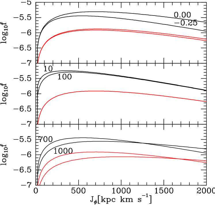
The top panel of Fig. 1 shows how the DF varies with for two pairs of values, and , of the power-law exponents and . Reducing the reduces the difference between the slopes of the black curves for circular orbits and the red curves for non-zero eccentricity and inclination. A large separation between the red and black curves implies a DF that falls rapidly with increasing eccentricity/inclination and thus small values of the velocity dispersions and . Hence reducing the increases the velocity dispersions at large radii relative to their values at small radii.
2.2 Observational significance of parameters
The real-space structure of a component depends on the gravitational potential in which it resides. In general that potential depends on all the model’s components, so it will change with any component’s parameters. Here in the interests of clarity we fix the potential, choosing the potential of a model that provides a good fit to observational data. Thus we adopt a very realistic potential and explore how the structure of a single component depends on the parameters in its DF.


2.2.1 Roles of the characteristic actions , and
The most important parameters are the three characteristic actions , where . While sets the component’s scale length, and set the in-plane and vertical dispersions, respectively. By setting these dispersions through and , we simultaneously determine a component’s vertical density profile and asymmetric drift through standard dynamics.
The upper panel of Fig. 2 shows the relationship between and and the velocity dispersions in the plane at . The lower panel shows that both dispersion satisfy quite accurately the relationship
| (6) |
where is the mean value of of the given disc’s stars sampled at . A relationship of this type is suggested by the fact that , where is some function on phase space: when we divide both sides by and average along an orbit , so when we further average over orbits we expect to find . This argument indicates that in the case , when the exponentials in the DF make the same throughout action space, velocity dispersions should fall in parallel with frequencies. In particular we expect to fall with increasing distance from the plane, and both ad to fall roughly as with distance from the Galactic centre.
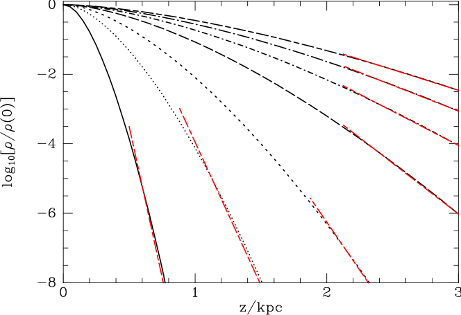
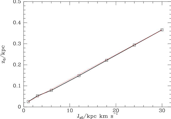
The upper panel of Fig. 3 shows the vertical density profiles of the components plotted in Fig. 2. The profiles steepen rapidly from zero in the plane to a nearly perfect exponentials once the density has fallen to less than a tenth of its central values. The lower panel of Fig. 3 plots the resulting asymptotic scale-height against . The relationship is almost exactly linear:
| (7) |


Fig. 4 shows how the vertical velocity dispersion in a disc component varies with height above the plane. The dispersion falls slowly as expected from the argument above relating to the mean frequency , while the density declines by orders of magnitude. The decline in is steepest near the mid-plane.
Fig. 5 shows the mean rotation speed (upper panel) and the radial velocity dispersion (lower panel) in a disc component at as functions of height. The radial velocity dispersions are to high precision independent of height. The thinnest components have, by construction, the smallest dispersions, so at they rotate fastest – they show the least asymmetric drift. In every component falls appreciably with height.
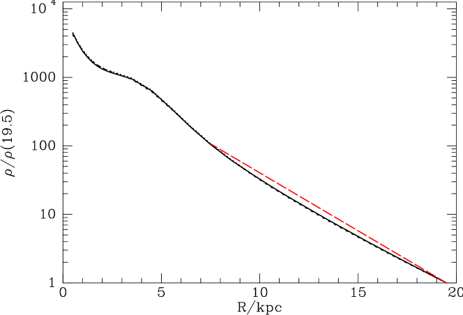
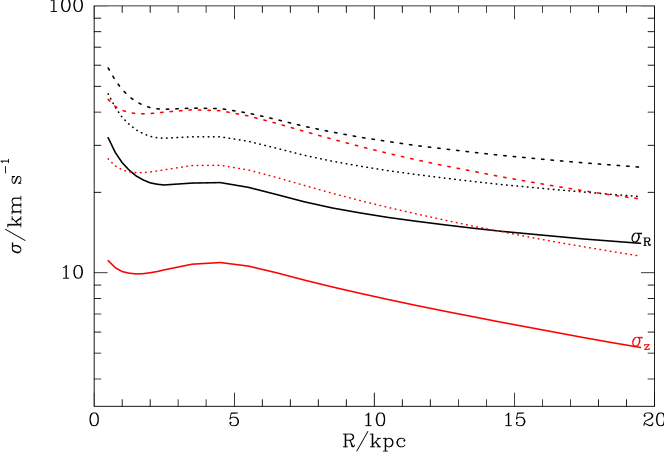
The upper panel of Fig. 6 shows the radial density profiles of the disc components with and . Beyond these profiles are quite accurately exponential with the common scale length that is indicated by the red dashed line. This scale-length is set by the value assigned to all components. Interior to the profiles acquire structure from the bulge via the self-consistently generated potential, as will be described below. Despite this structure, the profiles approximate exponentials at all .
The lower panel of Fig. 6 shows the dependence on radius of the velocity dispersions of these components in the radial (black) and vertical (red) directions. The ratio increases rapidly with disc thickness, approaching unity for the hottest disc plotted [which has ]. This result is a natural consequence of the decision to have span a smaller range () than (). In the thinnest disc (full curves) the vertical dispersion falls almost exponentially with , while the radial dispersion falls more slowly. This result reflects the fact that is much more sensitive than to the contribution of the disc to the overall gravitational field: around the density of the disc that generates the gravitational field used for these figures is declining nearly exponentially with .
2.2.2 Role of the exponents and
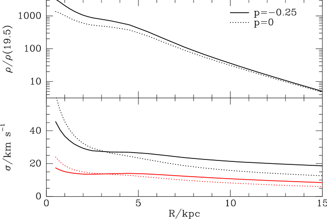
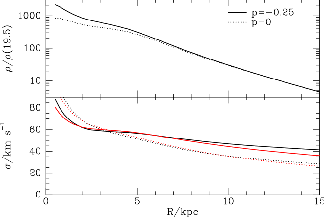
The exponents and that occur in equation (3) moderate the rates at which the and decrease outwards. The results plotted above are for . We will find that data for our Galaxy requires slightly negative values of , which cause and to decrease outwards more slowly.
In Fig. 7 we show the mid-plane density and velocity dispersions for (full curves) and in the case of a cold disc and a hot disc (lower pair of panels). Larger values of correspond to steeper outward gradients of the dispersions, as expected.
2.2.3 Role of the characteristic action
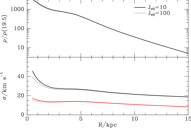
Fig. 8 shows the effect on a cold disc of increasing the characteristic action from to . This parameter is active only for non-zero , so Fig. 8 compares profiles for a disc with . As expected, has a perceptible effect only near the centre and in the sense that larger values lower the central velocity dispersions, and by hydrostatic balance, correspondingly increase the central mid-plane density. However, the effect on the plotted cold disc of even ten-fold decrease in is extremely small. The effect is no larger in the case of a hot disc.
3 Halo DFs
To build a self-consistent model Galaxy we require DFs for at least two hot components: the dark halo and the bulge / stellar halo. On account of the Galactic bar, a satisfactory model of the bulge would be non-axisymmetric so cannot be provided with our technology and we are obliged to model the bulge as an axisymmetric structure. Since few bulge stars reach the volume around the Sun in which the Gaia data are most precise, and the non-axisymmetric components of the bulge’s gravitational field decay strongly with increasing Galactocentric radius, we anticipate obtaining useful results even with a completely axisymmetric model.
For all three hot components of our Galaxy we employ a modified double power-law DF that is related to, but different from, those introduced by Posti et al. (2015) – hereafter P15. Our modifications of the P15 proposal are two-fold. First the phase-space density at the origin of action space is made finite by the mechanism introduced by Cole & Binney (2017). Second, the linear combination of actions that forms the basis of the P15 proposal is replaced by a more complex function of the actions. A full explanation of this replacement lies beyond the scope of this paper and will be presented elsewhere (Binney, 2022) but it addresses a weakness of the P15 proposal that was mentioned already by Binney & Piffl (2015), namely unphysical behaviour of velocity distributions at small .
The P15 halo DF is
| (8) |
Instead of the linear combinations and , we use
| (9) |
Here
| (10) |
with is a measure of an orbit’s circularity and
| (11) |
is a generalisation of the total angular momentum. The constants and in the definition of are chosen such that vanishes as . Specifically
| (12) |
where is a number grater or equal to unity. We allow to depend on energy by writing
| (13) |
where and are constants and is a dimensionless surrogate for energy that increases from zero at the origin of phase space to unity for marginally bound orbits through the formula
| (14) |
where and
| (15) |
where is a scale action.
When , and in a spherical potential the distributions of and are identical. If and are then set to the values suggested above, the velocity distribution becomes isotropic when and radially biased when . To flatten the component in a spherical potential, one sets and above unity. If the potential is flattened, setting , and and to the ratio of vertical to azimuthal epicycle frequencies at small and large radii, respectively causes the velocity distribution to be nearly isotropic.
4 Models of our Galaxy
In this section we use the DFs for disc components defined above to fit multi-component, self-consistent models to data for stars in the Gaia DR2 release (Gaia Collaboration & Brown, 2018) for which the Radial Velocity Spectrometer (RVS) measured line-of-sight velocities (Gaia Collaboration & Katz, 2018).
4.1 The data
We used the stellar locations and velocities computed by Schönrich et al. (2019) for the RVS stars. These authors adopted as the distance to the Galactic centre and as the Sun’s Galactocentric velocity. According to this assumption, the Sun is moving towards the Galactic centre, ahead of the local circular speed and up out of the plane. They determined a distance-dependent selection function of the RVS sample and used the kinematic method of Schönrich et al. (2012) to determine the offset of Gaia DR2 parallaxes. After determining this offset, they obtained moments for the probability distribution of the distance to each star using the Bayesian technique of Schönrich & Aumer (2017).
We restricted the sample to stars with quoted uncertainties smaller than a fifth of their parallax . The selection function of the RVS sample is complex (Everall et al., 2021) and a decision was taken not to engage with it in this preliminary work. From this decision it follows that we cannot attach significance to the number of stars listed in any spatial bin; only the distribution of these stars in velocity is significant.
| 0 | 0.1 | 0.2 | 0.35 | 0.5 | 1 | 1.75 | 3 |
We used the data given by Schönrich et al. (2019) to compute the histograms of Galactocentric velocity components , and for each of 35 spatial bins. These bins are defined by a rectangular grid in the plane that stretches from to and from the plane up to . Table 2 defines this grid.
4.2 Observational uncertainties
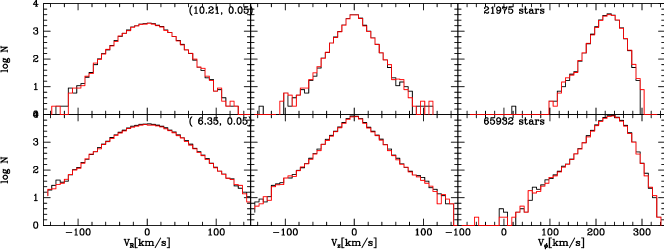
We investigated the impact of observational uncertainties on the histograms by drawing a sample from a realistic model using the approximation to the RVS selection function given by Schönrich et al. (2019) and comparing the histograms one obtains from the raw sample and from the sample after the stars have been scattered by the uncertainties in distance, proper motion and line-of-sight velocity. The uncertainties in each observable were averages of the DR2 uncertainties given for stars that lay at essentially the same distance from us – we used 50 equal-width bins in distance out to . We checked the correctness of the code by computing the differences between the observables before and after scattering and showing that the standard deviations of these differences agree with the uncertainties used to scatter the stars.
Errors in velocities will be most important for the most distant stars, so Fig. 9 shows their effect on the most distant bins, looking inward in the lower row of panels and outward in the upper row. The red histograms computed after scattering stars essentially obliterate the black histograms computed before scattering the raw sample. This perhaps surprising result allows us to neglect observational uncertainties even when using DR2 data, and in the following we compare histograms from Gaia with the model’s distribution of velocities at the barycentre of the Gaia stars in each bin. EDR3 data is superior to DR2 data in that its astrometric uncertainties are smaller, so if we upgraded to EDR3 data, more stars would pass our quality cuts so more stars would contribute to each histogram, and observational uncertainties would be even less significant. But given that our data/model comparisons are limited neither by Poisson noise nor by observational uncertainties, we continue to use the DR2 data.
4.3 The models
Our Galaxy models comprise eight components of which seven are defined by DFs and the eighth, the gas disc, is defined as a density distribution that contributes to the total potential. Following Dehnen & Binney (1998) the gas disc has density
| (16) |
with , , and . This gas disc has total mass , and at the solar radius has surface density and central density .
We include three spheroidal components – a dark halo, a bulge and a stellar halo – and four disc components – a thick disc and old (), middle-aged (), and young components () of the thin disc. Each of these discs has a DF of the type defined in Section 2, while the spheroidal components have DFs of the type defined in Section 3.
| Spheroids | Mass | |||||||||
| Dark halo | 98 | 100 | 10000 | 20000 | 1.6 | 2.7 | 2 | 1.4 | 1.2 | 100000 |
| Stellar halo | 0.1 | 5 | 600 | 100000 | 1 | 3.5 | 2 | 1.8 | 1.2 | 100000 |
| Bulge | 1.1 | 5 | 19.5 | 200 | 0.5 | 1.8 | 2 | 3 | 2 | 100000 |
| Discs | Mass | |||||||||
| Young disc | 0.175 | 650 | 10 | 0.65 | -0.7 | -0.3 | 10 | 100 | ||
| Middle disc | 0.75 | 600 | 17 | 2.8 | -0.35 | -0.1 | 10 | 700 | ||
| Old disc | 1.0 | 550 | 22 | 5 | -0.25 | -0.1 | 10 | 700 | ||
| Thick disc | 0.95 | 400 | 63 | 30 | 0.13 | 0.05 | 20 | 40 |

4.4 Fitting Gaia data
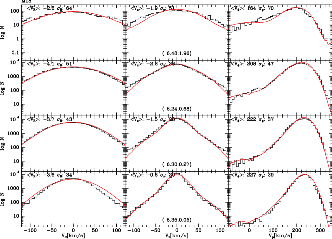
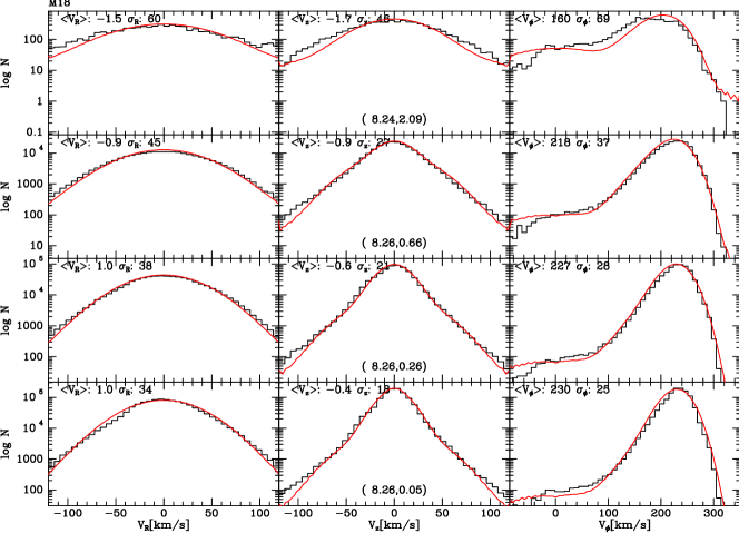
agama computes the density of each component on an appropriate grid (spherical for the dark halo and cylindrical for the stellar components) using an assumed potential, then it solves Poisson’s equation for the resulting potential and re-determines the density in this new potential. This sequence of potential determinations is quite rapidly convergent. An excellent first guess at the potential is generally available from the potential of the last model created, so on a good laptop a new model can be computed in only minutes. After computing the self-consistent potential, agama computes one-dimensional velocity distributions at 35 locations that are the barycentres of spatial bins into which the Gaia stars have been grouped. In Figs. 10 – 12 these locations are shown at the bottom of the panels – Table 2 gives the bin boundaries. The black histograms in Figs. 10 – 12 show the velocity distribution of RVS sample stars. We show histograms for only 12 of the 35 bins, being alternate bins in both and . The top left corner of each panel shows the mean and standard deviation of the histogram. The small, varying non-zero means of and must arise from a combination of the Galactic bar and non-equilibrium dynamics. The red curves in Figs. 10 – 12 show the velocity distributions computed by agama, normalised to the same number of stars as the corresponding black histogram.
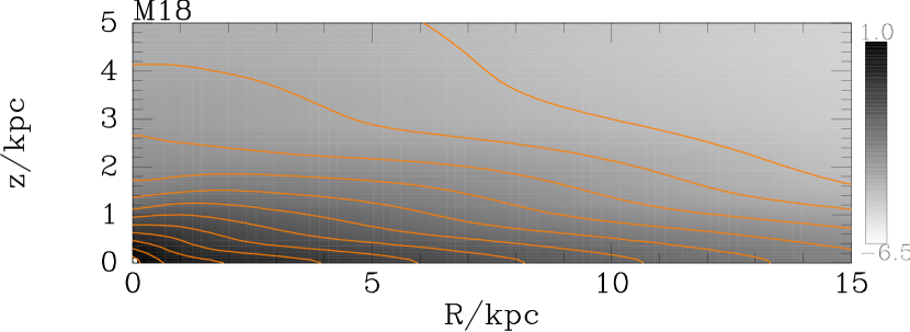
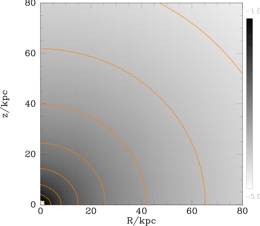
Experiments with automatic optimisation of the parameters by the Nelder-Mead downhill simplex algorithm (e.g. Press et al., 1986) were unsuccessful in that the machine proved unable to find a convincing DF in an acceptable number of iterations. It seems that the high dimension of the relevant parameter space combined with the cost of each model evaluation (which arises more from computation of diagnostics than from model construction) sets a requirement for a more sophisticated machine-learning algorithm than naive least-squares minimisation. Therefore we now present a model that has been fitted by hand to the Gaia data and the vertical stellar density profile of Gilmore & Reid (1983). Table 3 lists the values of the parameters that define the model. Fig. 13 shows the density of the stars and dark halo in the meridional plane.
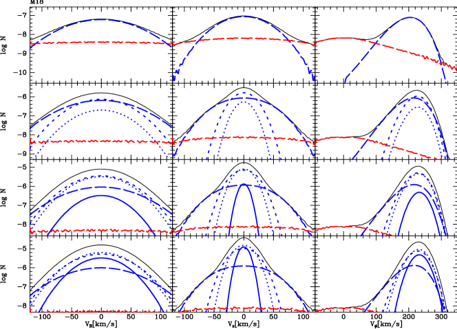
The lower block of panels in Fig. 11 breaks the model velocity histograms for the solar cylinder into the contributions of each stellar component. The full blue curve of the young disc only dominates at the core of the distribution, while the thick disc dominates in the wings and furthest from the plane everywhere except in the histogram, where at small the stellar halo dominates. The values of listed in Table 3 show a six-fold increase in between the thick disc and the old disc, whereas the characteristic actions that control the in-plane dispersions increase by a factor of six only between the young disc and the thick disc. Another noteworthy trend among the parameters are the steady increases in the values of and as one passes from the young disc to the thick disc. That is, the decrease outwards of the velocity dispersions is steeper in older components.
When fitting models by hand, velocity histograms like those shown in Figs. 10 to 12 yield numerous clues for parameter improvement. Most fundamentally, the location of the bumps in the histograms at bottom right indicate how good the model’s circular-speed profile is. This informs the choice of the normalisations of the principal components (dark halo, bulge, discs). The widths of the distributions shown in the left columns of Figs. 10 to 12 guide choices of the parameters of the disc DFs, with the youngest disc dominating the histograms for low (bottom left panels) and the thick disc dominating the histograms at top left. Any tendency for the model histograms to be less satisfactory at an inner radius than at an outer one is addressed by adjusting the relevant parameter. Similarly, the histograms guide choices of , and . Well above the plane, the model histograms have a flat section at low and a bump. The lower block of panels in Fig. 11 shows that the flat section is contributed by the stellar halo, while the bump is dominated by the thick disc. The balance between these two features guides choices of the normalisation of the stellar halo.
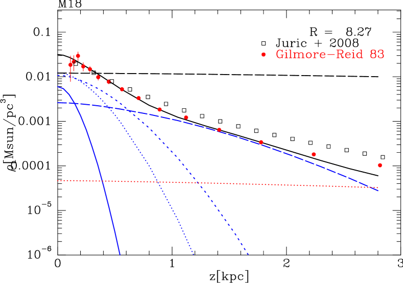
Further clues to parameter choice can be drawn from Fig. 14, which shows, in blue, the densities contributed at different distances from the plane by the disc components (full curve: young disc; dotted: middle-aged disc; short-dashed: old thin disc; long-dashed: thick disc). The dashed black and dotted red curves, show the contributions of the dark and stellar halos, respectively. The full black curve shows the sum of the stellar components, which may be compared with the data shown by red dots and black squares. The red points are from Gilmore & Reid (1983), while the black squares show the double-exponential fit of Jurić et al. (2008). Both sets of points can be shifted vertically at will. To make the full black curve pass through the red data points, one has to adjust the normalisations of the dark halo and the discs, and also the disc parameters , in the choice of which Fig. 11 provides additional guidance. Crucially, the middle panels of Figs. 10 to 12 effectively fix the parameters, so the only way to address the model density falling off too steeply with is to weaken the gravitational field near the plane by shifting mass from the disc to the dark halo. Hence, if the black squares from the SDSS survey were trusted more than the work of Gilmore & Reid (1983), one would make the dark halo more massive and the disc less massive.
Comparison of the red model predictions and the black Gaia histograms in Figs. 10 to 12 shows a considerable measure of agreement between the model and the data at each of the 12 locations shown; plots for the remaining 23 locations considered show a similar level of agreement.
4.4.1 Weaknesses of the fits
In the top-centre panels of Figs. 10 and 11, the red model curves are narrower than the black data curves. The only significant contributors to these curves are the thick disc, which dominates at , and the stellar halo. This problem might be addressed by reducing the thick disc’s value of .
In the bottom left panel of Fig. 10 the red model curve lies above the black data curve. The thick, middle and old discs all make significant contributions to the wings of these curves. The problem could be addressed by lowering for the middle disc at the risk of spoiling agreement in other panels.
In Figs. 10 to 12 the red curves for have a tendency to be too high at . It would be unwise to take the model’s predictions for stars of low too seriously because stars that approach the Galactic centre must be influenced by the Galactic bar, which is not included in the model. However, the model’s prediction of a surfeit of stars at is least apparent in Fig. 10 for the bins closest to the centre, where the bar should be most influential. The red curves for in the top-right panels of Figs. 10 to 12 are dominated by the stellar halo, which we have modelled as a non-rotating component because many studies (e.g. Schönrich et al., 2014, and references therein) have concluded that this is so. So perhaps one should revisit the issue of halo rotation in light of these Gaia data: the outer halo may be non-rotating (or even counter-rotating (Carollo et al., 2007)) but the inner halo may rotate detectably. In any event, ours is a very basic model of the stellar halo, that cannot address the empirical chemodynamical dichotomy into fairly isotropic, metal-poor and radially biased, metal-richer components (Helmi et al., 2018; Belokurov et al., 2018). Such a model must await resolution of the issue regarding choice of DFs discussed by Binney (2022).
4.4.2 Predictions of the models
| gas | stars | DM | Total | |
|---|---|---|---|---|
| 13.6 | 21.6 | 26.0 | 61.2 | |
| 0.057 | 0.0317 | 0.0121 | 0.0436 |
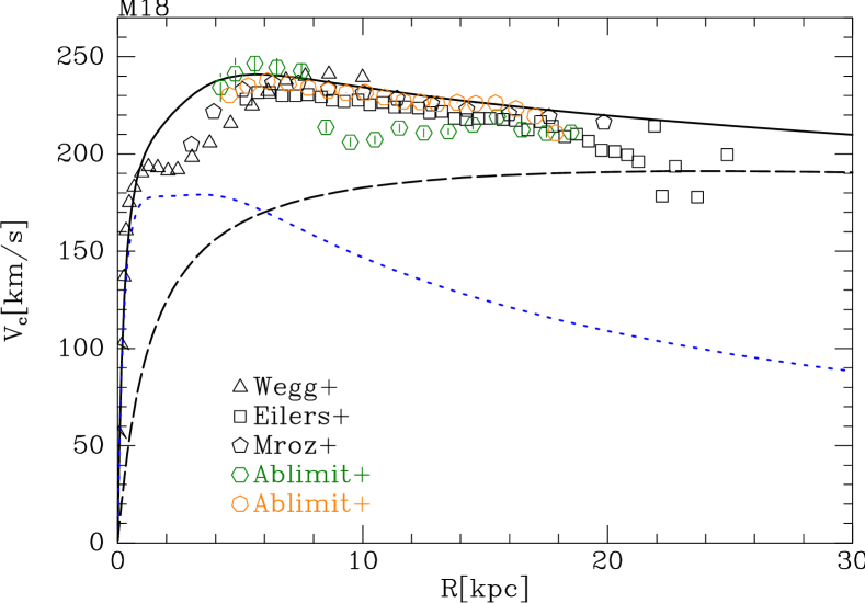
The full black curve in Fig. 15 shows the circular-speed curve of the gravitational potential that emerges from the choices made for the DF by the self-consistency condition. After optimising agreement between model and data in the earlier figures, the model does not have freedom to adjust this curve, so it is a significant result that it agrees remarkably well with the data points from other recent work, including the Wegg & Gerhard (2013) dynamical model of the bar/bulge, modelling of Cepheid variables by Mróz et al. (2019) and Ablimit et al. (2020) and a study of red giants by Eilers et al. (2019). In Fig. 15 the model curve is set by the kinematics of all stars in the restricted radial range rather than by objects presumed to be on near circular orbits over a wider range of radii. The curve extends in to the centre and out to large radii by virtue of the physical assumptions that underlie the functional forms of the DFs. It runs just above the majority of the data points, but this will to some extent reflect our adoption from Schönrich et al. (2019) of a faster value for the Sun’s component than others have used.
In Fig. 15 the dotted blue curve shows the contributions to from stars and gas. Baryons make the largest contribution to the circular-speed curve within and the bulge contributes more than the disc inside . In fact, in the inner kiloparsec the gravitational force from the disc is directed outwards, so it actually reduces – see below.
Table 4 gives the local densities of baryons and dark matter according to the model shown here, and also the surface density of mass that lies within of the plane at the solar radius. This comprises of gas, of stars and of dark matter. For comparison, Kuijken & Gilmore (1991), using a sample of K dwarfs, inferred , while Holmberg & Flynn (2004), using K giants as tracers, obtained . More recently, by counting stars in Gaia EDR3 Everall et al. (2022a) infer of stars, and by applying the Jeans equations to data from Gaia DR3 Nitschai et al. (2021) find .
Table 4 reports the model’s local density of stars to be , which lies below but is consistent with the value Everall et al. (2022a) inferred from Gaia EDR3. The local density of the stellar halo is . Table 4 reports the local density of dark matter to be . For comparison, from their study of red giants, Eilers et al. (2019) inferred the local density of dark matter to be , while Nitschai et al. (2021) obtained and Cautun et al. (2020) found . Thus our model is more dark-matter dominated than several recent studies prefer. Evidently we still have some way to go before a consistent picture emerges of the local structure of our Galaxy. A comprehensive review of estimates of the dark halo can be found in de Salas & Widmark (2021).
Given that the circular speed is falling at , there is scope for confusion in this area because the surface density within of the plane and the vertical acceleration satisfy
| (17) |
Often values of are quoted instead of . In the present model
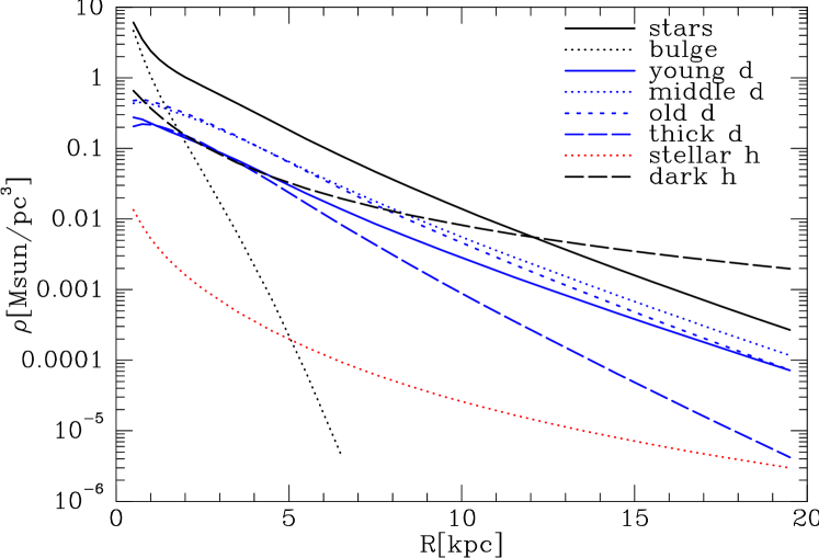


The full black curve in Fig. 16 shows the sum of the mid-plane densities of all the stellar components. It is very nearly exponential although comprised of contributions that have very different sale-lengths. The steep black, dotted line shows the nearly exponential density of the bulge. At the Sun the dark halo contributes a third of the density contributed by stars.
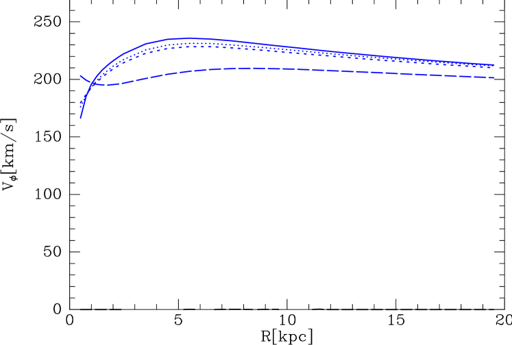
The lower panel of Fig 16 shows the mean-streaming speeds of the stellar discs at the mid-plane. For the thin-disc components is only slightly smaller than , while the value for the thick disc is generally reduced by an asymmetric drift in excess of .
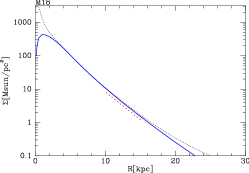
Fig. 17 shows what the Galaxy would look like when seen face-on. The solid blue curve in the left panel shows the contributions of the four disc components while the dotted black curve shows the density obtained on adding the contributions of the bulge and stellar halo. The profiles are not far from exponential.
The dashed red line shows the slope characteristic of a disc with a scale length , slightly larger than the value reported by Robin et al. (2003) from mid-IR photometry. There is a strong correlation between the disc’s scale length and degree of dark-matter domination in the sense that longer scale lengths imply less dark matter. This correlation is enforced by the radial variation of the circular speed, which is very tightly constrained by the histograms. If one assumes that the dark halo is not too dissimilar to the NFW model (see Section 4.5), then the gentle decline in at evident in Fig. 15 places an upper limit on the dark halo’s contribution that becomes tighter as grows, and, as explained at the end of Section 4.4, a massive disc is incompatible with the data for the vertical density profile shown in Fig. 14. Thus, ultimately the disc’s vertical density profile at sets .
The middle panel of Fig. 17 shows the rms thicknesses of the four disc components. All four components become thicker as one moves outwards. The right panel shows the projected line-of-sight velocity dispersions of the disc components, which all increase inwards. The steep central increases in the dispersions of the thin-disc components are associated with the central holes in their surface densities: the blue curves in left panel of Fig. 17 show that the surface density of the stellar discs rises in the inner kiloparsec before flattening, and starting to fall in earnest around . This structure causes the gravitational field of the stellar disc to be directed outwards near the centre. The gas disc, which has a central hole, amplifies this effect.
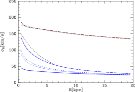
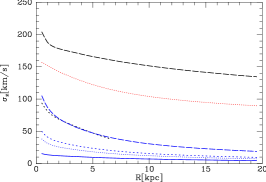
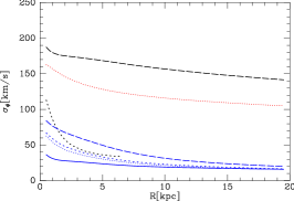
Fig. 18 shows the radial variation within the plane of the velocity dispersions. At small radii the dark halo has a weak tangential bias that is a consequence of its assumed adiabatic compression by the baryons, and the dispersions fall gently from at to at . The stellar halo (red dotted curves) is radially biased, with similar to the dispersions of the dark halo.
The black dotted curves in Fig. 18, which show the velocity dispersions of the bulge, show and tracking the dispersions of the thick disc, but falling much more steeply.
In all disc components . everywhere although invariably falls faster with increasing than does .
4.5 The halo without baryons
| Dark halo | 20.0 | 192 | 80.5 |
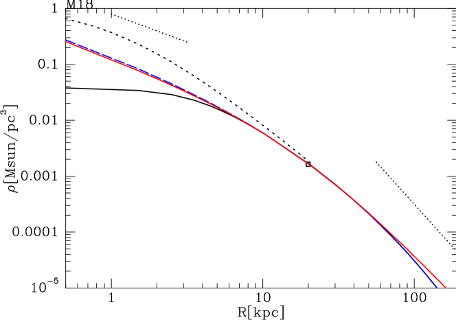
Our understanding of the statistical properties of dark haloes depend to a large extent on cosmological simulations that exclude baryons. Comparison of the Galaxy’s dark halo with expectations raised by such simulations requires knowledge of the structure of the dark halo before the baryons fell in. The classic assumption is that the accumulation of baryons was an adiabatic process (Blumenthal et al., 1986; Sellwood & McGaugh, 2005). In this case, the primordial structure of the dark halo can be recovered by constructing the self-consistent model defined by the dark halo’s DF alone. The full black curve in Fig. 19 shows the structure of this object.
There is now significant evidence that baryonic infall was significantly non-adiabatic (Chan et al., 2015; Pontzen & Governato, 2014; Pascale et al., 2018). Indeed it is natural that in the region in which baryons dominate the gravitational field, fluctuations in the gravitational field will have upscattered dark-matter particles, with the consequence that their phase-space density is now lower than it was before the baryons fell in. The Cole-Binney core of our halo is designed to model the consequences of this physics, so to obtain the best estimate of what the dark halo looked like before the baryons fell in, we should remove this core from the DF. The dashed blue curve in Fig. 19 shows the density profile of this primordial dark halo. It closely hugs the red curve, which plots the density of the NFW model that has the same scale radius (the radius at which ). This closeness of fit is no accident: the search for a dark halo DF was confined to ones that in isolation generate an NFW profile after removal of the Cole-Binney core. This curve yields for the radius at which the mean density is 200 times the mean cosmic density and for the mass interior to that radius. For comparison, Eilers et al. (2019) derive , while two estimates obtained by Ablimit et al. (2020) are and . When comparing these estimates one must bear in mind that the RVS data can constrain the density only at , so quoted values of even involve significant extrapolation and values of and are dangerously exposed to assumptions about the halo’s density profile – for example, the mass of our halo could be made larger either by increasing its truncation action or making its outer slope shallower. The globular cluster system provides some sensitivity to mass that lies beyond , and from a study of this system Wang et al. (2021) inferred . Using both globular clusters and dwarf spheroidal galaxies, and taking into account perturbation by the LMC, Correa Magnus & Vasiliev (2022) finds . Whereas ours estimates are based on a reconstruction of the dark halo prior to baryon infall, those of earlier work relate to models of the halo as it now is.
The dashed curve in the upper panel of Fig. 19 shows the dark halo’s current density profile; despite the upscattering of dark-matter particles, the gravitational pull of the baryons has more than tripled its density at from what it was even before the upscattering. The density enhancement remains significant out to . Comparing the current of the dashed and full black curves in the upper panel of Fig. 19 we see that the widespread assumption that the dark haloes of luminous galaxies have NFW profiles is indefensible. Dark haloes will have such profiles only if upscattering of dark-matter particles precisely cancels adiabatic compression, and there are no grounds for believing this to be true. For more on this topic, see Cautun et al. (2020).
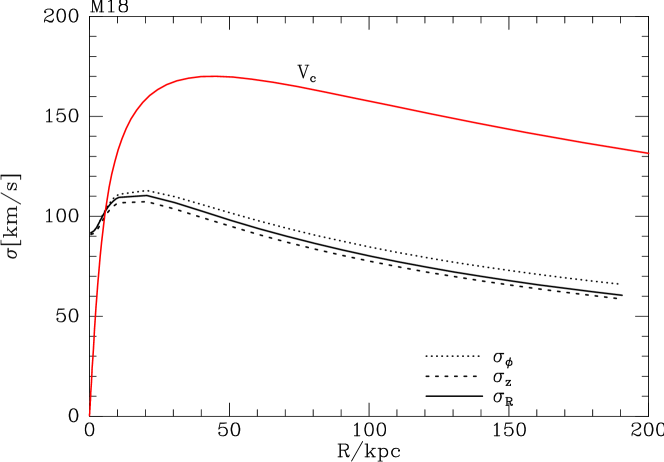
The lower panel of Fig. 19 plots velocities associated with this reconstruction of the primordial dark halo. Its circular speed, plotted in red, peaks at and its velocity distribution is nearly isotropic. Removal of the core changes the dispersions negligibly at .
4.6 Chemodynamics
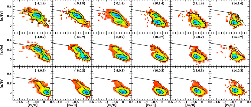
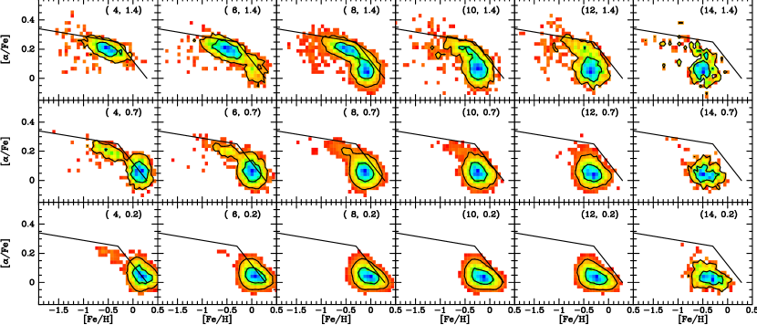
Fig. 4 of Hayden et al. (2015) is one of the most significant products of the APOGEE survey (Majewski et al., 2017). It shows the distribution of stars in the ([/Fe], [Fe/H]) plane in each of 18 bins in the plane. The robustness of this result was recently confirmed by Eilers et al. (2022). The upper block of panels in Fig. 20 is an analogous plot using the same data, kindly supplied by M. Hayden. Two stellar populations are clearly visible. There is a high- population that always occupies the same location in the chemical plane but is much more prominent at large and small : it has essentially disappeared at and is very faint at . The other, normal-, population dominates near the plane and at large . It moves to lower [Fe/H] with increasing .
If we conjecture how the stellar populations of our dynamical model are distributed in the chemical plane, we can create a analogous figure. The lower block of panels in Fig. 20 shows the result of doing this as follows.
| Component | ||||||||
|---|---|---|---|---|---|---|---|---|
| Young disc | - | - | ||||||
| Middle disc | - | - | ||||||
| Old disc | - | - | ||||||
| Thick disc | 0 | |||||||
| Stellar halo | 0 | - | - | |||||
| Bulge | 0 | - | - |
At the centre of each spatial bin we determined the fractional contribution to the stellar density by stars belonging to each of the six populations, young disc, middle disc, old disc, thick disc, stellar halo and bulge. Then mock stars were drawn from the velocity distributions of the components in the corresponding proportions, the total number of stars being the same as the number of real stars reported by Hayden et al. (2015) for that spatial bin. The mock stars were assigned values of [Fe/H] and [,Fe] by sampling its component’s chemical pdf. Each pdf was a two-dimensional Gaussian with principal axes
| (18) |
that are rotated with respect to the [Fe/H] and [/Fe] axes. The angle being small, is close to [Fe/H] while is close to [/Fe].
In the normal- components, the distribution in was independent of but the mean value of was taken to be
| (19) |
where is the circular angular momentum at the Sun and is approximately the mean metallicity of the component at . This dependence of on generates a metalliticy gradient in the disc.

The top row of Fig. 20 shows that the high- population is scarcely visible at . The obvious way to engineer this fading of the high- is to make the probability of a thick-disc star belonging to this population a function of . However experiments with of the form
| (20) |
produced results that were unsatisfactory in two respects: i) an implausibly rapid transition was required, specifically , and ii) it left the high- population too prominent at and . The more satisfactory results shown in the lower block of panels of Fig. 20 were obtained by taking the probability of belonging to the high- population to be
| (21) |
Now for and for . If a star was assigned to the high- portion of the thick disc, its chemistry was drawn from a Gaussian in independently of , while if it was assigned to the normal- disc, its chemistry was determined as if it were a member of the old disc. The upper panel of Fig. 21 is a plot of for the chosen values of and .
Table 6 lists for each component the numbers that define the two-dimensional Gaussians pdfs, and the parameters and that determine the distribution of high- stars within the thick disc. Comparison of the upper and lower blocks of panels in Fig. 20 shows that the model captures the essential features of the observations, including the dominance of the high- population at small and large , and the drift of the normal- population towards lower [Fe/H] with increasing .
5 Discussion
5.1 Extracting information from data
Much previous galaxy modelling has been based on the Jeans equations (Binney et al., 1990; Robin et al., 2003; Garbari et al., 2012; Read & Steger, 2017; Nitschai et al., 2020, 2021; Sivertsson et al., 2022). Gaia produces such lage samples that the full distribution of velocities in a small spatial region can be determined with exquisite precision. These distributions are highly non-Gaussian, so a technique which characterises them by just two or three moments is throwing away valuable information.
Extraction of the maximum information from a stellar survey is probably achieved by evaluating the likelihood of the survey data given candidate models. Unfortunately, this technique is unfeasible when there is significant obscuration by dust and the density of dust is not well known (e.g. Li & Binney, 2022b). Moreover, evaluating likelihoods for individual stars is very costly for samples as large as those yielded by Gaia. In light of these considerations there is a compelling case for binning stars spatially and evaluating the fit to models of the resulting velocity distributions. The comparison would be better made by evaluating likelihoods in velocity space than by binning stars by their single velocity components, but the cost of likelihood evaluation seems currently prohibitive. Humans can more easily assess fit quality from one-dimensional velocity distributions than from three-dimensional ones, but for an MCMC search of model space one should probably bin stars into cell in velocity space that are not the two-dimensional slices right across the space employed here.
5.2 The dark-matter baryon balance
Hand-fitting models to the data reveals a strong connection between the radial structure of the dark halo and the extent to which the disc is self-gravitating. On the one hand, the large distances from the plane reached by thick-disc stars places an upper limit on the disc’s mass. On the other hand, the clear outwards decline in the circular speed at requires both a significant contribution to the gravitational field from stars, and that the circular speed contributed by the dark halo does not rise strongly in this radial range. The latter requirement places an upper limit on the core parameter , and a lower limit on the index of the dark halo’s DF. It would be very interesting to use the MCMC algorithm to explore how big a region of model space acceptable models occupy.
5.3 We need better halo DFs
Action-based DFs that envisage a non-zero density of stars in the neighbourhood of need to conform to certain constraints (Piffl et al., 2015; Binney, 2022). The disc DFs introduced here have vanishing star densities at so do not need to engage with these constraints, but the spheroidal DFs of the dark halo, the bulge and the stellar halo should conform to these constraints, and they do so to only a limited extent. To avoid excessive violation of the constraints, and the introduction of unphysical features, the parameters of the spheroidal DFs have been chosen to avoid plausible levels of radial bias. The absence of radial bias in the dark halo and the bulge is not significant observationally because the data contain few bulge stars and no dark-matter particles. But the stellar halo needs to have greater radial bias and work to enable this should be a high priority. Moreover, restricting the velocity anisotropy of the dark halo’s DF limits the dark halo’s flattening, and a flattened halo will imply a less massive disc. Hence, better functional forms for spheroidal DFs may significantly change our understanding of the disc-halo balance.
5.4 Structure of the high- population
The quality of the fit to the Hayden et al. (2015) data that is provided by the restriction of high- stars to orbits with large is so good that it seems certain that the restriction is real, but its historical origin is far from evident. The a priori expectation is that high- stars would be restricted to low because these would be the first stars to form in the natural inside-out formation picture. However, fruitless attempts to model the data in this way left us convinced that it is to orbits with large that high- stars are confined.
In light of this result the high- population would form a very strange component if considered in isolation, for it comprises stars that have apocentres in that fall in quite a narrow range – the lower panel of Fig. 21 illustrates this fact by showing how the DF of this populaton depends on . It seems that at low the density of high- stars increases with , peaking where a star with turns around.
Could the -distribution of the high- stars have arisen when a primordial, high-, thin disc was shattered in a merger (Belokurov et al., 2020)? The problem with this idea is that we would expect the merger to spread stars in rather than shift them all up in , leaving orbits around vacant until occupied by the subsequent formation of low- stars. A possibly more promising scenario that the high- stars were stripped from a satellite that was finally disrupted on a nearly circular orbit, and their characteristic value of was the vertical action of the satellite when it dispersed. Another possibility is that we are seeing the result of ‘levitation’ (Sridhar & Touma, 1996): stars trapped in a resonance such as moving up in along with the resonance as the disc gains mass and the values of in the plane increase.
5.5 What to do with all Gaia stars
Gaia is a survey instrument that provides photometry of unprecedented precision. Hence it is the ultimate tool with which to determine how the density of stars varies with location. Yet we have completely neglected this possibility and instead used a forty-year-old determination of the density of stars above the Sun (Gilmore & Reid, 1983). The problem is that the Gaia catalogues have complex selection functions. Even after these selection functions have been determined (Everall & Boubert, 2022), to predict how many stars will be catalogued at a given sky position one needs accurate knowledge of the extinction as a function of distance along the relevant line of sight. This knowledge is currently woefully lacking for most sight lines, but fortunately along lines of sight at deg extinction is sufficiently low that a poor understanding of its distribution is not a major problem, so it is possible to deduce the vertical profile of the disc near the Sun from Gaia data, and Everall et al. (2022b, a) have recently done this. Their work appeared after the present work was largely completed and a decision was made not to replace the Gilmore & Reid (1983) data with the new determination of because it would be fundamentally sounder to fit the self-consistent models directly to Gaia’s star counts rather than to a density profile that has been fitted to the star counts – Everall et al. (2022b, a) needed to assume that the luminosity function is independent of , though it will not be because younger populations are more prominent at low , and older and more metal-poor populations dominate at high .
Since each population of the current models comes with an age range and therefore a luminosity function, predicting the star counts along a dust-free line of sight is straightforward. Comparison of these star counts, modified by the relevant Gaia selection function, with the actual star counts will then yield a constraint on the models that can replace that provided here by Fig. 14.
Probably the best way to use comparisons between predicted and actual Gaia star counts along general lines of sight is for the construction of a global three-dimensional dust map. Current attempts to construct dust maps are restricted to the tiny fraction of stars for which it is possible to obtain an extinction (Sale & Magorrian, 2014; Green, 2018; Green et al., 2019; Lallement et al., 2022). Such stars, mainly intrinsically blue stars, are for some reason susceptible to having their absolute magnitudes predicted. A model of the type presented here, combined with a trial dust model, yields for each field of view star counts as a function of parallax that can be compared with the actual star counts down to the faintest magnitudes. Hence every star in the Gaia catalogue can be used to constrain the dust model.
6 Conclusions
Fully self-consistent dynamical galaxy models constitute valuable tools for the interpretation of observational data for both our Galaxy and external galaxies because they pull constraints from a variety of observational probes into a coherent physical framework. They minimise the number of parameters that must be determined from observations by exploiting to the full the constraints imposed by the laws of dynamics.
Such models are inherently steady-state models, and currently agama can only construct axisymmetric models. However, from such a model one may easily draw an N-body sample, and by perturbing this either study time-dependent phenomena (e.g. Binney & Schönrich, 2018; Al Kazwini et al., 2022) or construct barred models by the made-to-measure technique (Syer & Tremaine, 1996; de Lorenzi et al., 2007).
Hitherto, self-consistent models of our Galaxy (Piffl et al., 2015; Binney & Piffl, 2015; Cole & Binney, 2017) have represented the discs with the quasi-exponential DF. Unfortunately, the radial and vertical epicycle frequencies and , and the circular radius play significant roles in this DF, so the DF is only fully specified when a potential is given. This fact makes the quasi-isothermal DF ill-suited to self-consistent galaxy modelling because the galaxy’s potential should emerge from the DF, not precede it.
Therefore in Section 2 we introduced a new family of DFs for discs that are fully specified by the disc’s mass and the values of seven parameters. We have elucidated the physical significance of the parameters: three characteristic actions set the scale length of the disc and the in-plane and vertical velocity dispersions. Two further parameters set the radial gradients of the dispersions and the final two control the central structure of the disc.
In Section 4 we built a model of our Galaxy that comprises four of these stellar discs, a gas disc, and three spheroidal components. The model reproduces to good accuracy the velocity distributions of stars in the Gaia RVS sample at 35 locations distributed through the rectangle and . It also fits old observations of the density of stars as a function of in the column above the Sun, which effectively set the balance between baryon and dark mass.
The model’s circular-speed curve is tightly constrained over the radial range covered by the Gaia RVS sample and it agrees well with recent determinations using specific tracer populations. Its stellar disc has mass , scale length and local surface density . Its dark halo has mass , scale radius and local density . Its original central cusp is assumed to have been eroded by interactions with baryons. We reconstructed the dark halo prior to baryon infall. Prior to the addition of baryons it had peak circular speed and virial radius .
The model’s stellar disc is a superposition of three relatively cool “thin” discs of increasing velocity dispersions and therefore thickness, and a much hotter and thicker disc. The disc’s scale lengths decrease as their dispersions and thicknesses increase. The hotter a disc is, the faster its velocity dispersions fall off with increasing radius.
After assigning a chemical composition to each of the model’s six stellar components, we could predict from the model how the chemistry of stars varies with location in the plane. We identified simple compositions of the components that yielded good agreement between the model’s predictions and the chemistry measured by the APOGEE survey (Hayden et al., 2015). The key feature of these compositions is the restriction of high- stars to orbits with high . This restriction ensures that normal- stars dominate both at low and small , and at high and large .
The Galaxy model presented here is designed mainly to illustrate the opportunities that are opened up by the new disc DFs. There is much scope to extend the work by a wider exploration of model space and the addition of more and better observational constraints.
Here we have presented a single model that provides good fits to most of the data. Attempts to find a best-fitting model were unsuccessful on account of the high dimensionality of the model parameter space and the cost of computing observables from a model. Nevertheless, soon the MCMC algorithm should be used to explore model space starting from this model and thus to obtain insight into the range of model parameters that generate acceptable models.
Acknowledgements
This work was supported by the UK Science and Technology Facilities Council under grant number ST/N000919/1. JB also acknowledges support from the Leverhulme Trust through an Emeritus Fellowship. We thank Michael Hayden for providing the APOGEE data re-plotted in Fig. 20.
This work presents results from the European Space Agency (ESA) space mission Gaia. Gaia data are being processed by the Gaia Data Processing and Analysis Consortium (DPAC). Funding for the DPAC is provided by national institutions, in particular the institutions participating in the Gaia MultiLateral Agreement (MLA). The Gaia mission website is https://www.cosmos.esa.int/gaia. The Gaia archive website is https://archives.esac.esa.int/gaia.
DATA AVAILABILITY
The code that generates Galaxy models can be downloaded from the agama website https://github.com/GalacticDynamics-Oxford/Agama
References
- Abazajian et al. (2003) Abazajian K. et al., 2003, AJ, 126, 2081
- Ablimit et al. (2020) Ablimit I., Zhao G., Flynn C., Bird S. A., 2020, ApJL, 895, L12
- Al Kazwini et al. (2022) Al Kazwini H. et al., 2022, A&A, 658, A50
- Antoja et al. (2018) Antoja T. et al., 2018, Nat, 561, 360
- Belokurov et al. (2018) Belokurov V., Erkal D., Evans N. W., Koposov S. E., Deason A. J., 2018, MNRAS, 478, 611
- Belokurov et al. (2020) Belokurov V., Sanders J. L., Fattahi A., Smith M. C., Deason A. J., Evans N. W., Grand R. J. J., 2020, MNRAS, 494, 3880
- Binney (2010) Binney J., 2010, MNRAS, 401, 2318
- Binney (2012) Binney J., 2012, MNRAS, 426, 1328
- Binney (2014) Binney J., 2014, MNRAS, 440, 787
- Binney (2022) Binney J., 2022, in preparation, xxx
- Binney & McMillan (2011) Binney J., McMillan P., 2011, MNRAS, 413, 1889
- Binney & Piffl (2015) Binney J., Piffl T., 2015, MNRAS, 454, 3653
- Binney & Schönrich (2018) Binney J., Schönrich R., 2018, MNRAS, 481, 1501
- Binney et al. (1990) Binney J. J., Davies R. L., Illingworth G. D., 1990, ApJ, 361, 78
- Blumenthal et al. (1986) Blumenthal G. R., Faber S. M., Flores R., Primack J. R., 1986, ApJ, 301, 27
- Boubert & Everall (2020) Boubert D., Everall A., 2020, MNRAS, 497, 4246
- Bovy & Rix (2013) Bovy J., Rix H.-W., 2013, ApJ, 779, 115
- Carollo et al. (2007) Carollo D. et al., 2007, Nat, 450, 1020
- Cautun et al. (2020) Cautun M. et al., 2020, MNRAS, 494, 4291
- Chan et al. (2015) Chan T. K., Kereš D., Oñorbe J., Hopkins P. F., Muratov A. L., Faucher-Giguère C. A., Quataert E., 2015, MNRAS, 454, 2981
- Cole & Binney (2017) Cole D. R., Binney J., 2017, MNRAS, 465, 798
- Correa Magnus & Vasiliev (2022) Correa Magnus L., Vasiliev E., 2022, MNRAS, 511, 2610
- de Lorenzi et al. (2007) de Lorenzi F., Debattista V. P., Gerhard O., Sambhus N., 2007, MNRAS, 376, 71
- de Salas & Widmark (2021) de Salas P. F., Widmark A., 2021, Reports on Progress in Physics, 84, 104901
- Dehnen & Binney (1998) Dehnen W., Binney J., 1998, MNRAS, 294, 429
- Eilers et al. (2019) Eilers A.-C., Hogg D. W., Rix H.-W., Ness M. K., 2019, ApJ, 871, 120
- Eilers et al. (2022) Eilers A.-C., Hogg D. W., Rix H.-W., Ness M. K., Price-Whelan A. M., Mészáros S., Nitschelm C., 2022, ApJ, 928, 23
- Everall et al. (2022a) Everall A., Belokurov V., Evans N. W., Boubert D., Grand R. J. J., 2022a, MNRAS, 511, 3863
- Everall & Boubert (2022) Everall A., Boubert D., 2022, MNRAS, 509, 6205
- Everall et al. (2021) Everall A., Boubert D., Koposov S. E., Smith L., Holl B., 2021, MNRAS, 502, 1908
- Everall et al. (2022b) Everall A., Evans N. W., Belokurov V., Boubert D., Grand R. J. J., 2022b, MNRAS, 511, 2390
- Gaia Collaboration et al. (2021) Gaia Collaboration et al., 2021, A&A, 649, A8
- Gaia Collaboration & Brown (2018) Gaia Collaboration, Brown A. G. A. e. a., 2018, A&A, 616, A1
- Gaia Collaboration & Katz (2018) Gaia Collaboration, Katz D. e. a., 2018, A&A, 616, A11
- Garbari et al. (2012) Garbari S., Liu C., Read J. I., Lake G., 2012, MNRAS, 425, 1445
- Gilmore & Reid (1983) Gilmore G., Reid N., 1983, MNRAS, 202, 1025
- Green (2018) Green G. M., 2018, Journal of Open Source Software, 3, 695
- Green et al. (2019) Green G. M., Schlafly E., Zucker C., Speagle J. S., Finkbeiner D., 2019, ApJ, 887, 93
- Hayden et al. (2015) Hayden M. R. et al., 2015, ApJ, 808, 132
- Helmi et al. (2018) Helmi A., Babusiaux C., Koppelman H. H., Massari D., Veljanoski J., Brown A. G. A., 2018, Nat, 563, 85
- Holmberg & Flynn (2004) Holmberg J., Flynn C., 2004, MNRAS, 352, 440
- Hunt et al. (2019) Hunt J. A. S., Bub M. W., Bovy J., Mackereth J. T., Trick W. H., Kawata D., 2019, MNRAS, 490, 1026
- Jurić et al. (2008) Jurić M. et al., 2008, ApJ, 673, 864
- Kuijken & Gilmore (1991) Kuijken K., Gilmore G., 1991, ApJL, 367, L9
- Lallement et al. (2022) Lallement R., Vergely J. L., Babusiaux C., Cox N. L. J., 2022, arXiv e-prints, arXiv:2203.01627
- Li & Binney (2022a) Li C., Binney J., 2022a, MNRAS, 510, 4706
- Li & Binney (2022b) Li C., Binney J., 2022b, arXiv e-prints, arXiv:2205.01455
- Majewski et al. (2017) Majewski S. R. et al., 2017, AJ, 154, 94
- Malhotra (1995) Malhotra S., 1995, ApJ, 448, 138
- Mróz et al. (2019) Mróz P. et al., 2019, ApJL, 870, L10
- Nitschai et al. (2020) Nitschai M. S., Cappellari M., Neumayer N., 2020, MNRAS, 494, 6001
- Nitschai et al. (2021) Nitschai M. S., Eilers A.-C., Neumayer N., Cappellari M., Rix H.-W., 2021, ApJ, 916, 112
- Pascale et al. (2018) Pascale R., Posti L., Nipoti C., Binney J., 2018, MNRAS, 480, 927
- Piffl et al. (2014) Piffl T. et al., 2014, MNRAS, 445, 3133
- Piffl et al. (2015) Piffl T., Penoyre Z., Binney J., 2015, MNRAS, 451, 639
- Pontzen & Governato (2014) Pontzen A., Governato F., 2014, Nat, 506, 171
- Posti et al. (2015) Posti L., Binney J., Nipoti C., Ciotti L., 2015, MNRAS, 447, 3060
- Press et al. (1986) Press W. H., Flannery B. P., Teukolsky S. A., 1986, Numerical recipes. The art of scientific computing. Cambridge: University Press, 1986
- Read & Steger (2017) Read J. I., Steger P., 2017, MNRAS, 471, 4541
- Reid & Brunthaler (2004) Reid M. J., Brunthaler A., 2004, ApJ, 616, 872
- Robin et al. (2003) Robin A. C., Reylé C., Derrière S., Picaud S., 2003, A&A, 409, 523
- Sale & Magorrian (2014) Sale S. E., Magorrian J., 2014, MNRAS, 445, 256
- Schönrich et al. (2014) Schönrich R., Asplund M., Casagrande L., 2014, ApJ, 786, 7
- Schönrich & Aumer (2017) Schönrich R., Aumer M., 2017, MNRAS, 472, 3979
- Schönrich et al. (2012) Schönrich R., Binney J., Asplund M., 2012, MNRAS, 420, 1281
- Schönrich et al. (2019) Schönrich R., McMillan P., Eyer L., 2019, MNRAS, 487, 3568
- Sellwood & McGaugh (2005) Sellwood J. A., McGaugh S. S., 2005, ApJ, 634, 70
- Sellwood et al. (2019) Sellwood J. A., Trick W. H., Carlberg R. G., Coronado J., Rix H.-W., 2019, MNRAS, 484, 3154
- Sivertsson et al. (2022) Sivertsson S. et al., 2022, MNRAS, 511, 1977
- Sridhar & Touma (1996) Sridhar S., Touma J., 1996, Science, 271, 973
- Steinmetz & et al. (2006) Steinmetz M., et al., 2006, AJ, 132, 1645
- Syer & Tremaine (1996) Syer D., Tremaine S., 1996, MNRAS, 282, 223
- Trick et al. (2019) Trick W. H., Coronado J., Rix H.-W., 2019, MNRAS, 484, 3291
- Vasiliev (2019) Vasiliev E., 2019, MNRAS, 482, 1525
- Wang et al. (2021) Wang J., Hammer F., Yang Y., 2021, Monthly Notices of the Royal Astronomical Society, 510, 2242
- Wegg & Gerhard (2013) Wegg C., Gerhard O., 2013, MNRAS, 435, 1874