A 1.46–2.48 $\mu$m Spectroscopic Atlas of a T6 Dwarf (1060 K) Atmosphere with IGRINS: First Detections of H₂S and H₂, and Verification of H₂O, CH₄, and NH₃ Line Lists

Abstract

We present Gemini South/IGRINS observations of the 1060 K T6 dwarf 2MASS J08173001$-$6155158 with unprecedented resolution ($R\equiv\lambda/\Delta\lambda=45\,000$) and signal-to-noise ratio (SNR$>$200) for a late-type T dwarf. We use this benchmark observation to test the reliability of molecular line lists used up-to-date atmospheric models. We determine which spectroscopic regions should be used to estimate the parameters of cold brown dwarfs and, by extension, exoplanets. We present a detailed spectroscopic atlas with molecular identifications across the $H$ and $K$ bands of the near-infrared. We find that water (H₂O) line lists are overall reliable. We find the most discrepancies amongst older methane (CH₄) line lists, and that the most up-to-date CH₄ line lists correct many of these issues. We identify individual ammonia (NH₃) lines, a hydrogen sulfide (H₂S) feature at 1.5900 $\mu$m, and a molecular hydrogen (H₂) feature at 2.1218 $\mu$m. These are the first unambiguous detections of H₂S and H₂ in an extra-solar atmosphere. With the H₂ detection, we place an upper limit on the atmospheric dust concentration of this T6 dwarf: at least 500 times less than the interstellar value, implying that the atmosphere is effectively dust-free. We additionally identify several features that do not appear in the model spectra. Our assessment of the line lists is valuable for atmospheric model applications to high-dispersion, low-SNR, high-background spectra, such as an exoplanet around a star. We demonstrate a significant enhancement in the detection of the CH₄ absorption signal in this T6 dwarf with the most up-to-date line lists.

1 Introduction

Reliable determinations of the effective temperatures, radii, and masses of isolated, self-luminous brown dwarfs and giant exoplanets are dependent on accurate modelling of their spectra. However, it is known that the laboratory-based experimental line lists used to generate model spectra are inconsistent with each other and are even missing lines for some molecular species (e.g., Saumon et al. 2012; Canty et al. 2015). Even the most up-to date spectral models do not completely reproduce observed spectral features in cold brown dwarfs, limiting our ability to constrain their basic properties.

Methane and ammonia are of particular interest for T dwarfs. At the time of their discovery, the distinction between L and T dwarfs was based on whether methane lines were present in low-resolution ($R\equiv\lambda/\Delta\lambda\sim 100$) spectra (Oppenheimer et al., 1995; Geballe et al., 1996). Similarly, ammonia was used to mark the end of the T-sequence and is the distinguishing opacity source of Y dwarfs (Cushing et al., 2011). Noll et al. (2000) have since shown that the onset of methane absorption occurs as early as L5 in $R\approx 600$ near-infrared spectra, and Cushing et al. (2006) report the appearance of ammonia bands at spectral type T2 in the mid-infrared. In the latest T dwarfs (T8, T9), ammonia becomes a major opacity source (Cushing et al., 2006).

Previous spectroscopic studies of late-T and Y dwarfs with broad wavelength coverage have been limited to $R=6000$ or less, making the identification of specific molecular absorption features difficult. Additionally, older generations of photospheric models have not been able to fit the available data well (e.g., Bochanski et al. 2011; Leggett et al. 2012, 2019; Beichman et al. 2014; Canty et al. 2015; Schneider et al. 2015; Luhman & Esplin 2016; Miles et al. 2020; Tannock et al. 2021).

A current hurdle in characterizing cold brown dwarfs and giant exoplanets are systematic uncertainties in the wavelengths and strengths of absorption lines in theoretical photospheres. Missing lines or inaccurate line lists make detections of molecules and determinations of radial velocities and projected rotation velocities difficult or impossible, especially in low signal-to-noise observations of exoplanet atmospheres. It is therefore necessary to confirm the accuracy of line lists by comparing to high signal-to-noise observations. Isolated brown dwarfs, free from the overwhelming light of a companion star, have atmospheres containing some of the key opacity sources in exoplanets, making them suitable laboratories for testing the accuracy of line lists. Improvements in the atmospheric opacity estimates for cold substellar atmospheres would also be invaluable for the characterization of potentially habitable exoplanets. Methane and ammonia have been suggested as biosignature gases in exoplanet atmospheres (e.g., Léger et al. 1996; Seager et al. 2013). Water, while not a biosignature gas, is also an important signature of habitability and is a major opacity source in brown dwarfs.

We present a high signal-to-noise (SNR $>$ 200) spectrum of a T6 dwarf with unprecedented $R=45\,000$ resolution and 1.45–2.48 $\mu$m coverage, observed with the Immersion GRating INfrared Spectrometer (IGRINS; Yuk et al. 2010; Park et al. 2014; Mace et al. 2016, 2018) on Gemini South. We perform a detailed study of absorption features due to water, methane, ammonia, carbon monoxide, and hydrogen sulfide. Our target, 2MASS J08173001$-$6155158 (also known as DENIS J081730.0-615520; hereafter 2M0817) was discovered by Artigau et al. (2010) through a photometric cross match between the Two Micron All Sky Survey (2MASS) and the DEep Near-Infrared Survey of the Southern sky (DENIS) point-source catalogues, and spectroscopically identified as a T6 dwarf. It is at a heliocentric distance of only 5.2127 $\pm$ 0.0113 pc (Gaia Collaboration, 2016, 2021), and is one of the brightest late-type T dwarfs ($K$-band magnitude 13.52; Skrutskie et al. 2006). Radigan et al. (2014) find a rotation period of 2.8 $\pm$ 0.2 h for 2M0817 from ground-based $J$-band observations spanning four hours.

2 Spectroscopy with IGRINS on Gemini South

We observed 2M0817 with IGRINS on Gemini South under Gemini program ID GS-2018A-Q-304 (PI: M. Tannock). IGRINS is a high-resolution ($R=45\,000$), cross-dispersed spectrograph that simultaneously covers the $H$ and $K$ bands from 1.45 to 2.48 $\mu$m.

Observations took place over four nights in April and May 2018 while IGRINS was on Gemini South. The slit was oriented at the default position angle of 90 degrees (east-west) for IGRINS, and exposures were taken along an ABBA dither pattern. We observed an A0 V star before or after each observation of the target at a similar airmass, with the same telescope and instrument configuration. We summarize these observations in Table 1.

Table 1: Gemini South/IGRINS Spectroscopic Observations of 2MASS J08173001$-$6155158 under Gemini program ID GS-2018A-Q-304 (PI: M. Tannock). The given SNR values are for the final, combined spectra. The FWHM of the trace includes both atmospheric seeing and effects from telescope and instrument optics. Typical atmospheric seeing at Gemini South is 0.5″.

Date	Exposure	Exposure	Target	Telluric	Telluric	$H$-band	$K$-band	FWHM of the
Observed	Time	Sequence	Airmass	A0 V	Standard	SNR (at	SNR (at	Trace in the
	(s)			Standard	Airmass	1.589 $\mu$m)	2.101 $\mu$m)	$H$ Band (″)
2018 Apr 5	1200	AB	1.18–1.20	HIP 40621	1.14	85	44	0.9
2018 Apr 5	600	ABBA	1.20–1.25	HIP 35393	1.28	63	34	0.9
2018 May 7	600	ABBA	1.22–1.28	HIP 36489	1.31	56	33	0.8
2018 May 22	518	ABBAAB	1.27–1.37	HIP 40621	1.36	174	112	0.6
2018 May 22	518	ABBAAB	1.40–1.58	HIP 40621	1.58	181	113	0.6
2018 May 23	518	ABBAAB	1.26–1.37	HIP 40621	1.35	184	119	0.6

2.1 Data Reduction

The data were reduced with Version 2 of the IGRINS Pipeline Package (PLP; Lee et al. 2017), at each epoch individually. The PLP performs sky subtraction, flat-fielding, bad-pixel correction, aperture extraction, wavelength calibration, and telluric correction. The PLP outputs wavelength-calibrated, telluric-corrected fluxes and the signal-to-noise ratio (SNR) for each point in the spectrum. For each observing epoch, the wavelength solution was derived from a combination of OH emission lines and telluric absorption lines. OH emission lines in the observed spectrum were removed through A–B pair subtraction, and telluric absorption lines were removed by dividing the target spectrum by an A0 V standard spectrum. The target spectrum was also multiplied by a standard Vega model to remove any features from the A0 V standard itself.

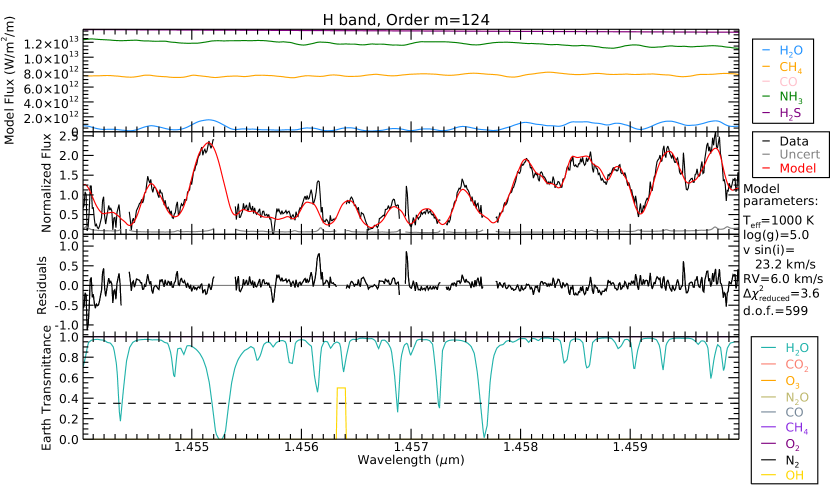
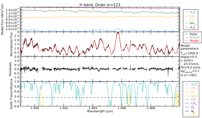
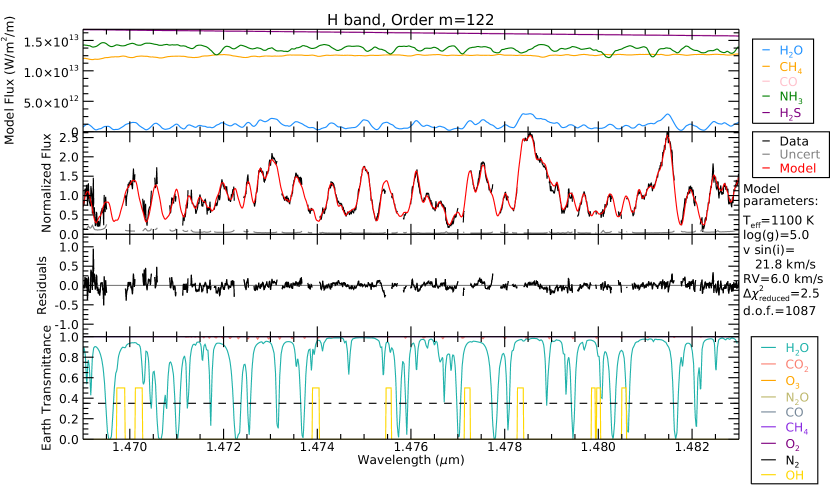
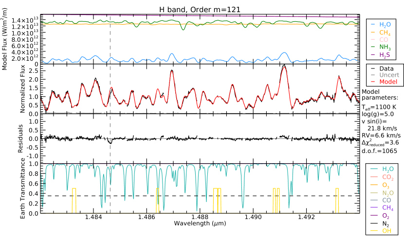
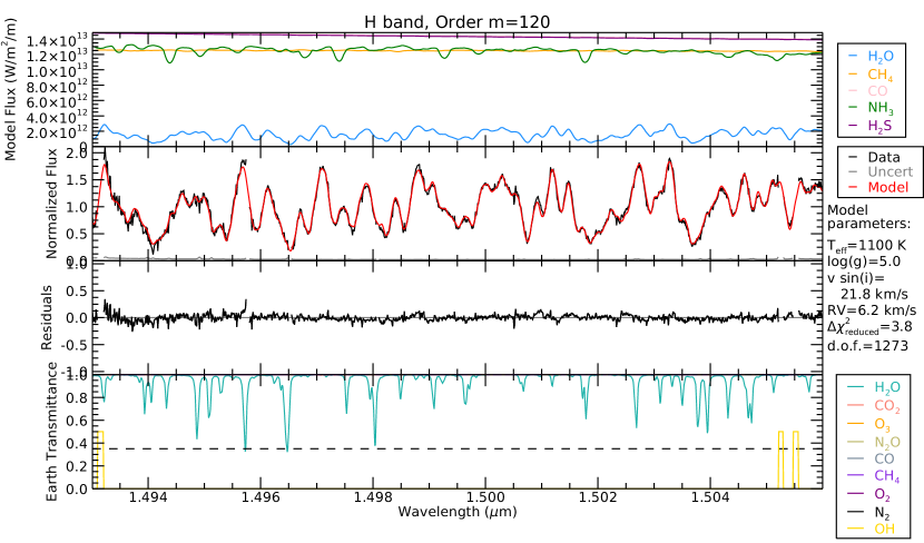
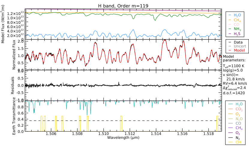
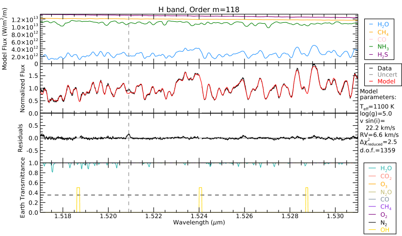
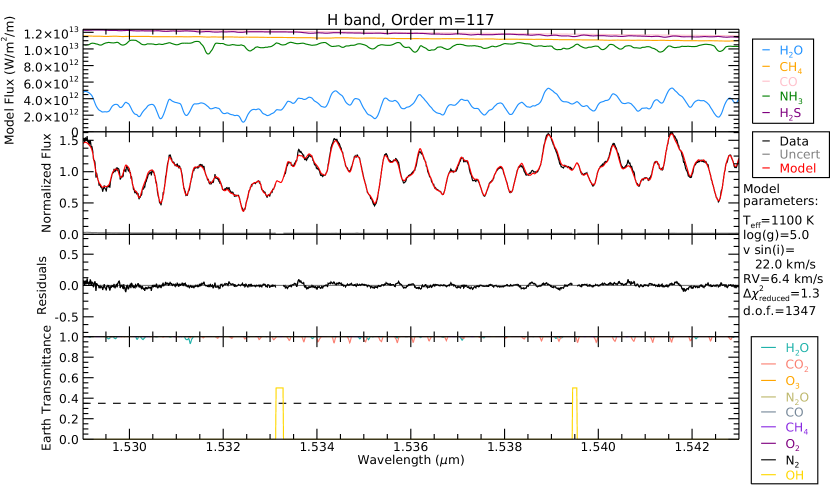
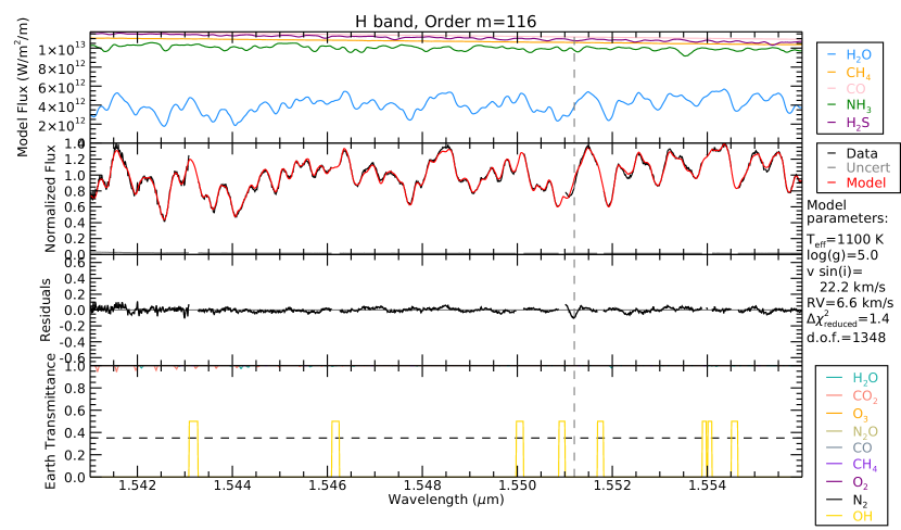
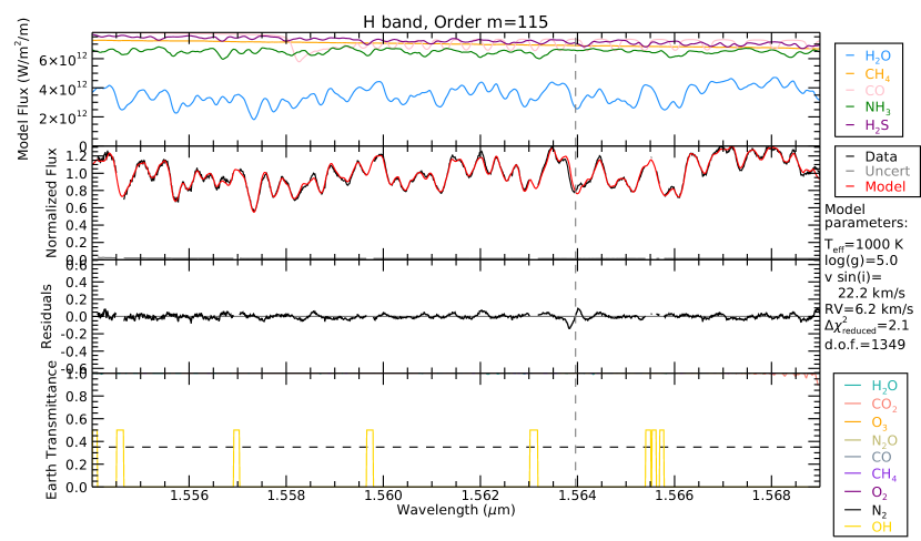
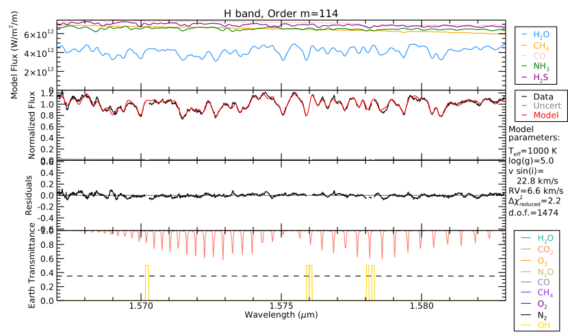
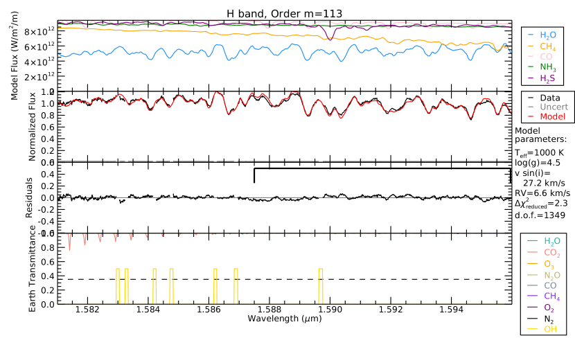
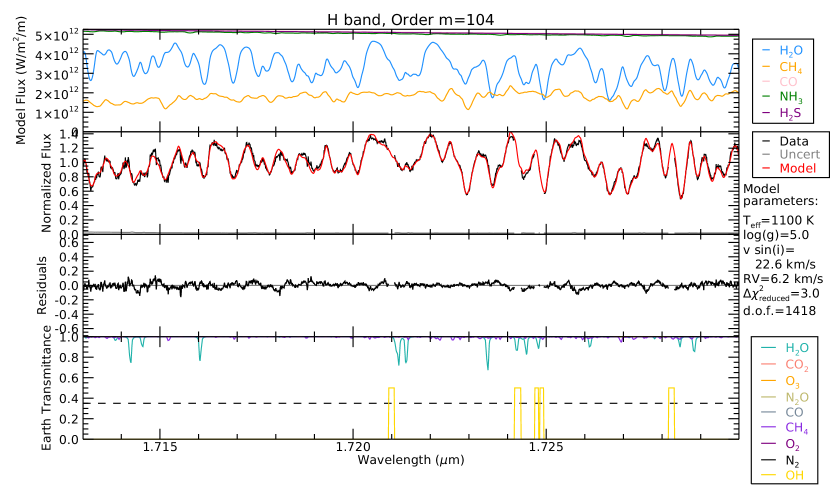
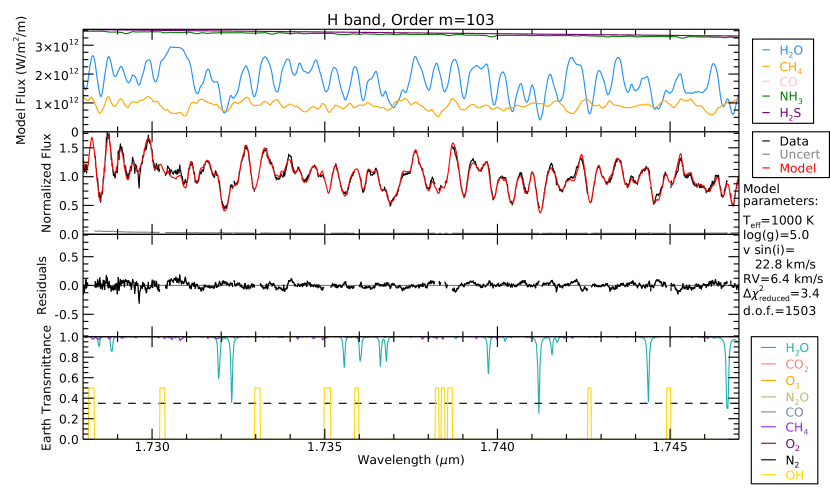
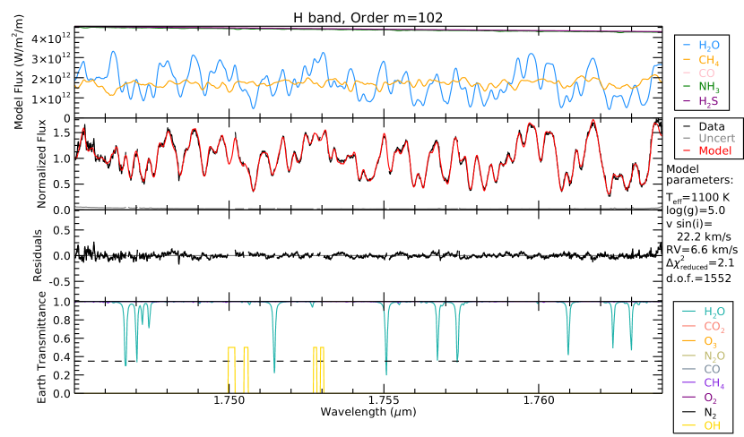
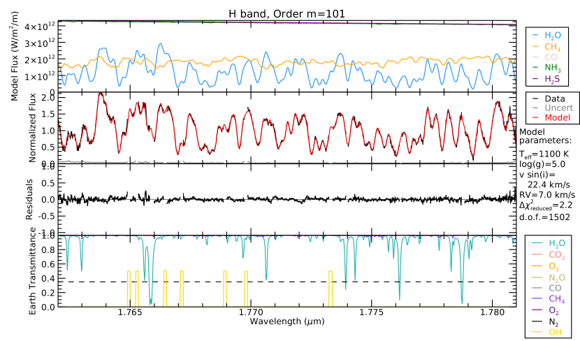
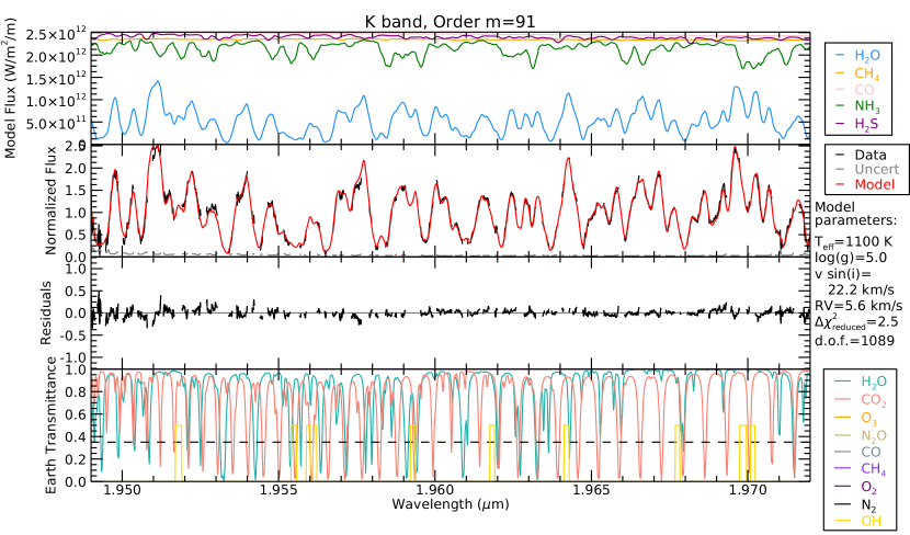
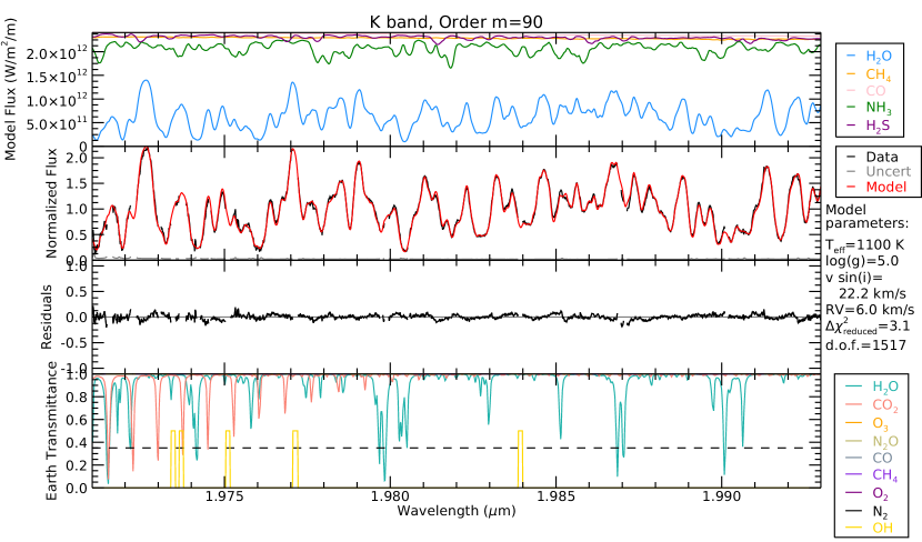
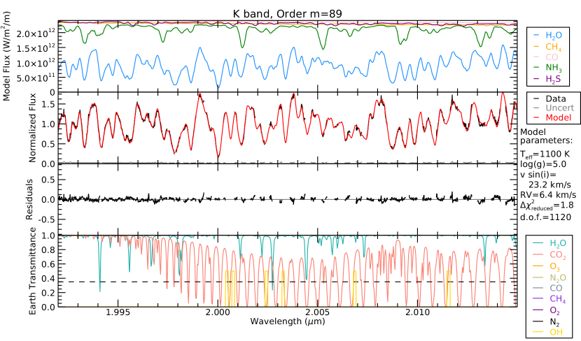
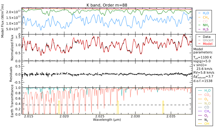
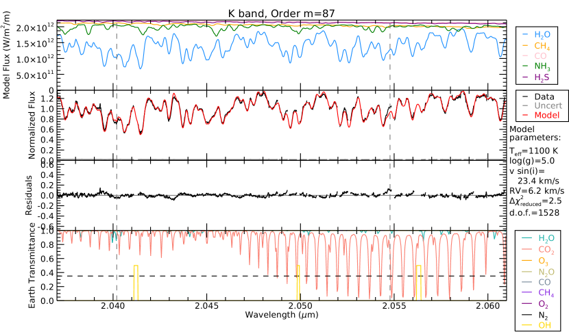
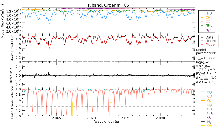
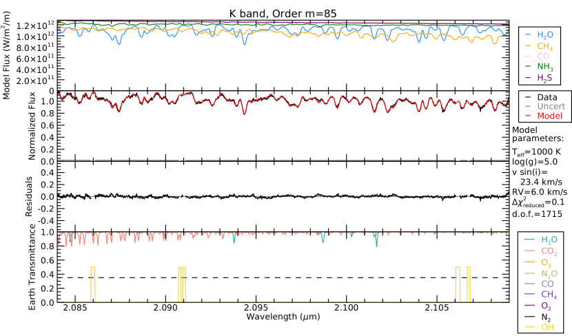
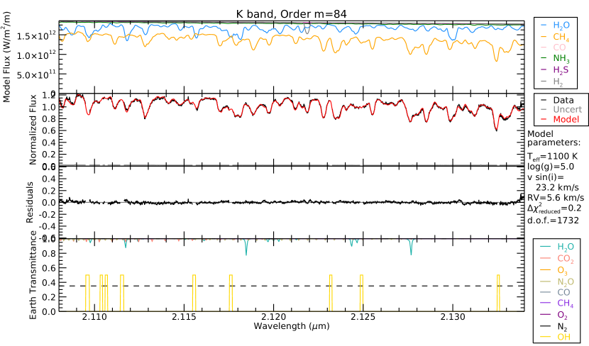
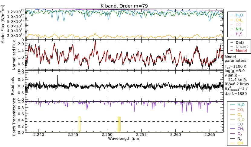
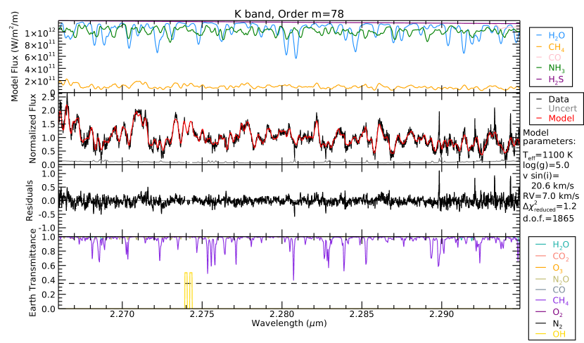
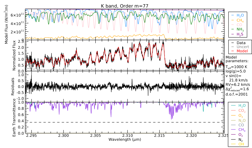
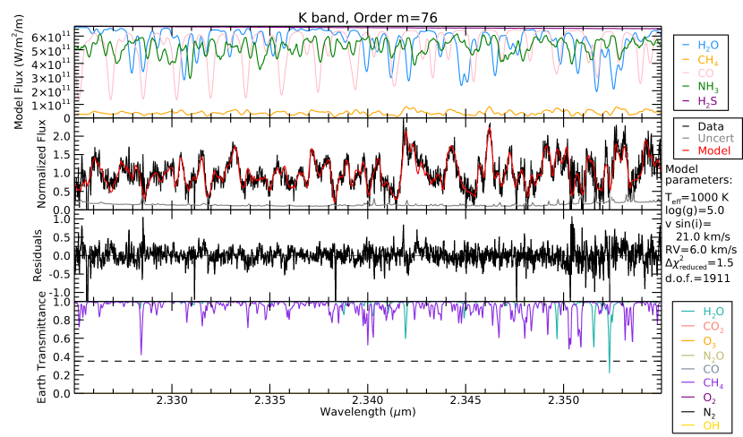
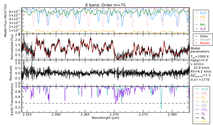
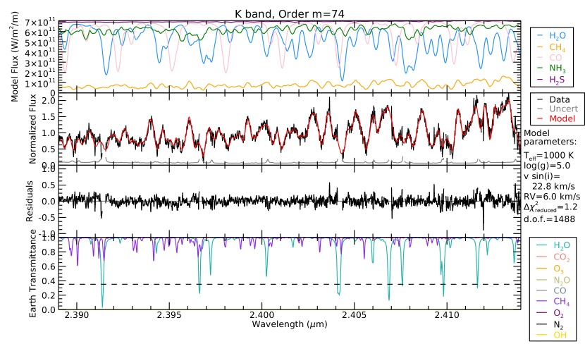
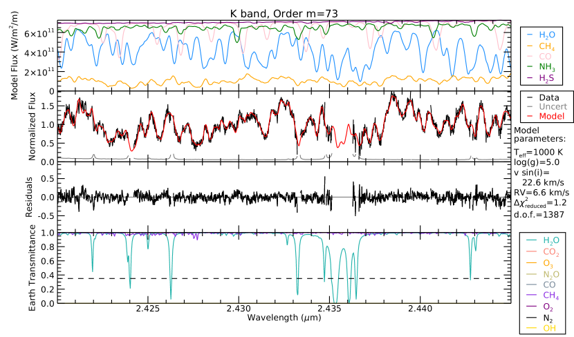
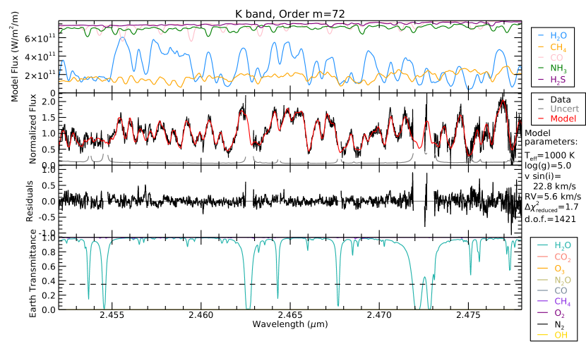
We found that the strongest telluric features were not completely removed in our data reduction, and left residuals that affected the chi square statistic ($\chi^{2}$) when comparing to models (Section 3). To identify and mask strong telluric features, we generated transmission spectra for the Earth’s atmosphere with the Planetary Spectrum Generator (PSG; Villanueva et al. 2018). We used the Earth’s Transmittance template with the longitude, latitude, and altitude of the Gemini South Observatory. We found that masking atmospheric lines with $>$ 65 per cent absorption strengths in the PSG Earth transmittance spectrum, along with strong OH emission lines (identified from the atlas of Rousselot et al. 2000) significantly improved the quality of our model photosphere fits. The PSG spectra and the 65 per cent absorption threshold beyond which we masked features are shown in the Figures of the Appendix.

We used a custom IDL code to combine the individual spectra. We first corrected for the barycentric velocity at each epoch. We then processed the $H$ and $K$ bands separately: we normalized the flux to peak at unity in each of the $H$ and $K$ bands, and then resampled the data to identical wavelength values. We computed the weights from the SNR values computed by the PLP ($w_{i}=(SNR_{i}/f_{i})^{2}$), where $f_{i}$ is the flux at each epoch) and computed the weighted average ($\bar{f}=\sum_{i=1}^{N}(f_{i}w_{i}/w_{t})$) where $w_{t}$ is the sum of the weights for $N$ epochs) and uncertainties ($\sigma=w_{t}^{1/2}$) across all epochs.

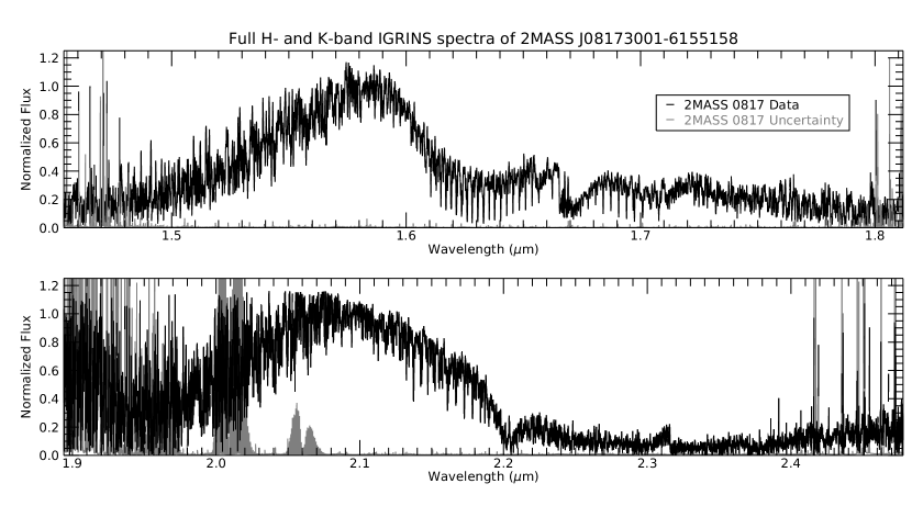
We found that in some cases, the IGRINS PLP produced fluxes of $\sim$0, but with disproportionately high SNR values, resulting in large weights. This produced large downward spikes in the weighted average spectrum. We obtained the highest SNR combined spectrum free of such spikes when we combined the three highest SNR epochs: 2018 May 22 (both sequences) and 2018 May 23. In Fig. 1 we show the data from each epoch in an order at the centre of the $H$ band. Three of the nights stand out with their higher SNR. We performed the remainder of our analysis with the weighted average of these three epochs. Our final combined spectrum (Fig. 2) had a signal-to-noise of $\sim$300 at the peak of the $H$ band and $\sim$200 at the peak of the $K$ band.

Figure 1: A sample order near the centre of the $H$ band, showing spectra from each of the six observing epochs. The normalized flux is shown in the top panel, and the deep absorption features in this order are due to H₂O. The SNR is shown in the bottom panel. The SNR of the neighbouring orders are also shown in grey, to show that IGRINS has good SNR coverage at all wavelengths. The IGRINS instrument transmission profile (blaze) is imprinted on the SNR spectrum, and is the reason for the fall-off in SNR at the edges of the order. The three highest-SNR spectra, obtained on 2018 May 22 and 23, were combined to create the final spectrum shown in Fig. 2.

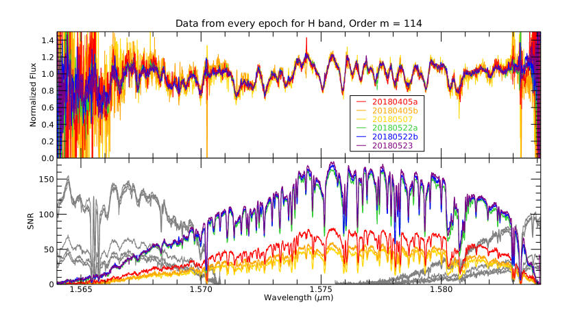
There is some overlap between the orders in the spectrum (see Table 2 for a list of the orders and their wavelength coverage). For our analysis, we analysed each order individually. The instrument blaze profile results in the short-wavelength ends of the order having lower SNR than the long-wavelength ends (see the bottom panel of Fig. 1). We show the complete spectra with the orders stitched together in Fig. 2. For this stitched spectrum, in each region of overlap, we averaged the fluxes from the two orders.

2.2 Confirmation of Wavelength Calibration

We verified our wavelength calibration by comparing the telluric lines in the spectra of our A0 V standard stars to the Earth’s transmittance spectrum from the PSG, generated over the wavelength coverage of IGRINS at 1.5 times the resolution of IGRINS. In each IGRINS order, between five and ten lines spread over the order were selected (very deep lines and blended lines were avoided), and we measured the wavelength at the minimum flux for each of these lines. We found an average offset of less than half an IGRINS pixel (0.110 Å at the centre of the $H$ band), confirming our wavelength calibration.

Figure 2: The full $H$- and $K$-band IGRINS spectra of 2MASS J08173001$-$6155158 with epochs combined and the orders stitched together. This figure does not include the quadratic correction described in Section 3.1. These data appear noisy, but in fact have SNR $\simeq$ 300 at the peak of the $H$-band spectrum and SNR $\simeq$ 200 at the $K$-band peak. The apparent noise spikes are all absorption features, and can be seen in detail in the full set of figures in the Appendix.

3 Model Fitting and Parameter Determination

We compared our observed spectra to the models of Allard et al. (2012, 2014, hereafter, BT-Settl), Morley et al. (2012, hereafter, Morley), Marley et al. (2021, hereafter, Sonora Bobcat), and an alternative version of the Sonora Bobcat models with updated molecular line lists from Hood et al. (in preparation, hereafter, Bobcat Alternative A). The BT-Settl models are based on the PHOENIX code (Allard & Hauschildt, 1995; Hauschildt et al., 1999). The latter three model sets are all based on the same 1D radiative-convective equilibrium model atmosphere code (e.g., Marley et al. 1996; Fortney et al. 2008; Marley & Robinson 2015). The Morley models include the effect of clouds that may be relevant for T dwarf atmospheres by applying the Ackerman & Marley (2001) cloud model. In contrast, the Sonora Bobcat models assume a cloud-free atmosphere. The Sonora Bobcat models include post-2012 updates to the gas opacity database, described in Freedman et al. (2014), Lupu et al. (2014), and Marley et al. (2021). The Bobcat Alternative A models are thermal emission spectra generated from the Sonora Bobcat atmospheric structures with the code described in the Appendix of Morley et al. (2015). Only a selection of opacities, that dominate at near infrared wavelengths, are included: H₂O, CH₄, CO, NH₃, H₂S, and collision-induced opacity of H₂-H₂, H₂-He, and H₂-CH₄. The opacity data for these sources are the same as the Sonora Bobcat models, with the notable exceptions of updated H₂O (Polyansky et al., 2018), CH₄ (Hargreaves et al., 2020), and NH₃ (Coles et al., 2019) line lists.

3.1 Fitting of Photospheric Models

The models are provided on fixed grids of effective temperature ($T_{\rm eff}$) and surface gravity ($\log g$, with $g$ in units of cm s^-2), and we do not interpolate between models to intermediate values. We allowed our model fitting to explore $T_{\rm eff}$ grids between 700 K and 1300 K (the expected range of 900–1100 K in $T_{\rm eff}$ for a T6 dwarf, $\pm$200 K; Filippazzo et al. 2015), in steps of 50 K or 100 K, depending on the model family. For $\log g$ we explored grids between $\log g=4.0$ and 5.5, in steps of 0.5 dex for all model families except the Sonora Bobcat models, which are in steps of 0.25 dex. The Morley models also have a sedimentation efficiency ($f_{\rm sed}$) parameter on a grid from 2 to 5 in integer steps.

We explored a radial velocity (RV) grid by applying a Doppler shift to the wavelength of the models. We also expect that our observed spectrum will have significant rotational broadening from its known axial rotation. We explored a grid of projected rotation velocities ($v\sin i$), by simulating rotational broadening in the model spectra. We convolved the model spectra with the standard rotation kernel from Gray (1992), as described in Tannock et al. (2021). For both RV and $v\sin i$ we first explored coarse grids with steps of 2 km s^-1 over a broad range of values, then narrowed our grid and repeated the fitting with finer steps of 0.1 km s^-1. After shifting and broadening the model spectra, we resampled the model spectra to the wavelengths of the observed spectrum using IDL’s interpol function.

We also observed an instrumental effect resulting in an upward curving in the residuals when compared to models at the ends of the orders. To minimize this effect and analyse the highest SNR regions of the data, we removed the ends of each order, leaving $\sim$1–2 nm overlap between orders. We additionally divided out a quadratic function that minimized the $\chi^{2}$ statistic between the data and the model to further remove this instrumental effect. With these corrections we obtained the $\chi^{2}$ values as:

$$\chi^{2}=\sum_{i=1}^{N}\left(\frac{O_{i}/(a\lambda^{2}+b\lambda+c)-M_{i}}{\sqrt{\sigma_{i}^{2}+\sigma_{M}^{2}}}\right)^{2},$$ (1)

where $O_{i}$ is the observed flux, $M_{i}$ is the flux of the model, $\sigma_{i}$ is the uncertainty of the data, $\sigma_{M}$ is a systematic uncertainty assigned to the model, and $\lambda_{i}$ is the wavelength of the corresponding data point. The coefficients of the quadratic correction are $a$, $b$, and $c$. Following a similar process to the one described in Suárez et al. (2021), we set the partial derivatives of Equation 1 to zero and solved the resulting system of equations to find the values of $a$, $b$, and $c$. We determined the coefficients of the quadratic for every model on the model grid individually.

We identified the best-fitting order of the entire spectrum (order $m=85$ of the $K$ band for the Bobcat Alternative A model) and determined the value of $\sigma_{M}$ that produced a reduced $\chi^{2}$ statistic of 1.0. The adopted value of $\sigma_{M}$ was approximately half of the average uncertainty of the data. This systematic uncertainty was added in quadrature to the observational uncertainties in every order. As a final measure of the goodness of fit for each order, in our figures we report the $\Delta\chi^{2}_{\rm reduced}$ with respect to the minimum $\chi^{2}_{\rm reduced}=1$ value for the best-fitting order. That is, for the best-fitting ($m=85$) order the goodness of fit is $\Delta\chi^{2}_{\rm reduced}=0$, while for orders with poorer fits, the goodness of fit is $\Delta\chi^{2}_{\rm reduced}=\chi^{2}_{\rm reduced}-1$.

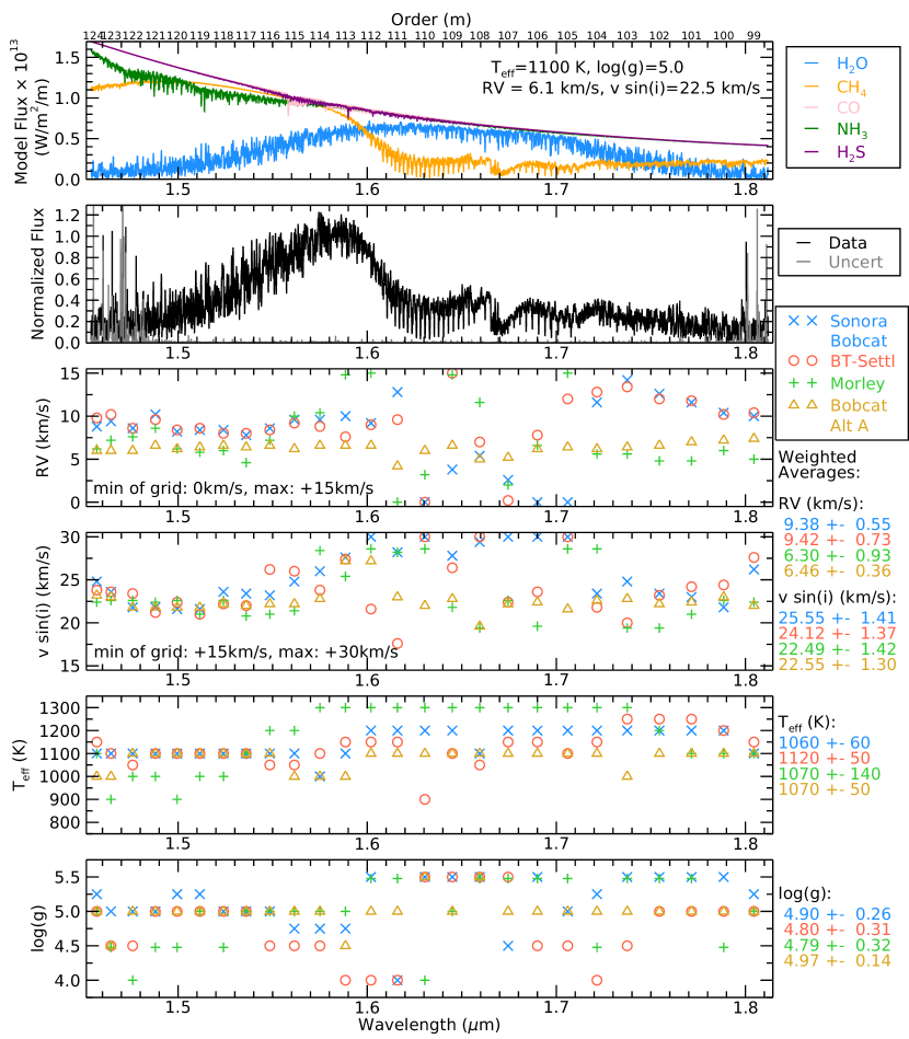
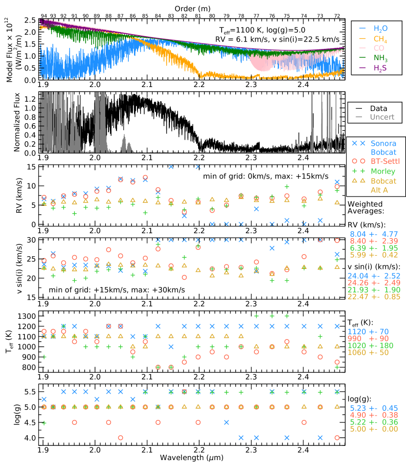
The total uncertainty, including the systematic uncertainty added in quadrature, is shown in grey in Fig. 3 and in all following figures, including in the Appendix. The total uncertainty is still very small in most orders, and appears indistinguishable from the wavelength axis in most figures, as our estimated S/N ratios can be well over 100. Nevertheless, we believe the overall uncertainties to be this small based on the above $\chi^{2}$ analysis.

Table 2: The wavelengths of the IGRINS orders and the major molecular absorbers in each order. Diffraction order numbers, $m$, were extrapolated from Stahl et al. (2021).

Band	Order	Wavelength	Major	Band	Order	Wavelength	Major
	($m$)	Coverage ($\mu$m)	Absorbers		($m$)	Coverage ($\mu$m)	Absorbers
$H$	124	1.454–1.460	H2O	$K$	94	1.894–1.910	H2O
$H$	123	1.459–1.470	H2O	$K$	93	1.909–1.930	H2O
$H$	122	1.469–1.483	H2O	$K$	92	1.929–1.950	H2O
$H$	121	1.482–1.494	H2O	$K$	91	1.949–1.972	H2O, NH3
$H$	120	1.493–1.506	H2O	$K$	90	1.971–1.993	H2O, NH3
$H$	119	1.504–1.519	H2O, NH3	$K$	89	1.992–2.015	H2O, NH3
$H$	118	1.517–1.531	H2O	$K$	88	2.014–2.038	H2O, NH3
$H$	117	1.529–1.543	H2O	$K$	87	2.037–2.061	H2O, NH3
$H$	116	1.541–1.556	H2O	$K$	86	2.060–2.085	H2O, CH4, NH3
$H$	115	1.554–1.569	H2O, CO	$K$	85	2.084–2.109	H2O, CH4
$H$	114	1.567–1.583	H2O	$K$	84	2.108–2.134	H2O, CH4, H2
$H$	113	1.581–1.596	H2O, CH4, H2S	$K$	83	2.133–2.159	H2O, CH4
$H$	112	1.594–1.610	H2O, CH4	$K$	82	. 2.158–2.185	CH4
$H$	111	1.608–1.624	H2O, CH4	$K$	81	2.184–2.212	CH4, NH3
$H$	110	1.622–1.639	H2O, CH4	$K$	80	2.211–2.239	CH4
$H$	109	1.637–1.653	H2O, CH4	$K$	79	2.238–2.267	CH4
$H$	108	1.651–1.668	H2O, CH4	$K$	78	2.266–2.295	H2O, CH4
$H$	107	1.666–1.683	H2O, CH4	$K$	77	2.294–2.326	H2O, CH4, CO
$H$	106	1.681–1.699	H2O, CH4	$K$	76	2.325–2.355	H2O, CH4, CO
$H$	105	1.697–1.715	H2O, CH4	$K$	75	2.354–2.383	H2O, CH4, CO
$H$	104	1.713–1.730	H2O, CH4	$K$	74	2.389–2.414	H2O, CH4, CO
$H$	103	1.728–1.747	H2O, CH4	$K$	73	2.420–2.445	H2O, CH4, CO
$H$	102	1.745–1.764	H2O, CH4	$K$	72	2.452–2.478	H2O, CH4
$H$	101	1.762–1.781	H2O, CH4
$H$	100	1.779–1.798	H2O, CH4
$H$	99	1.797–1.812	H2O, CH4

3.2 Determination of Physical Parameters

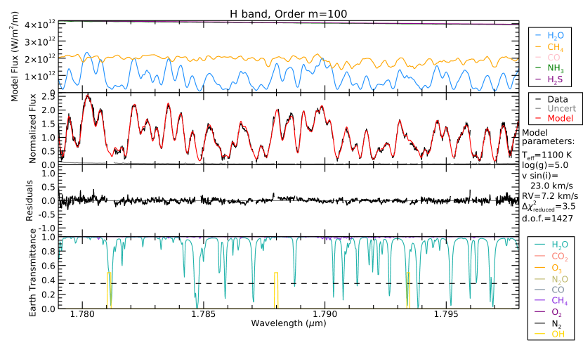
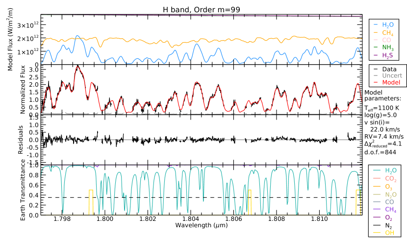
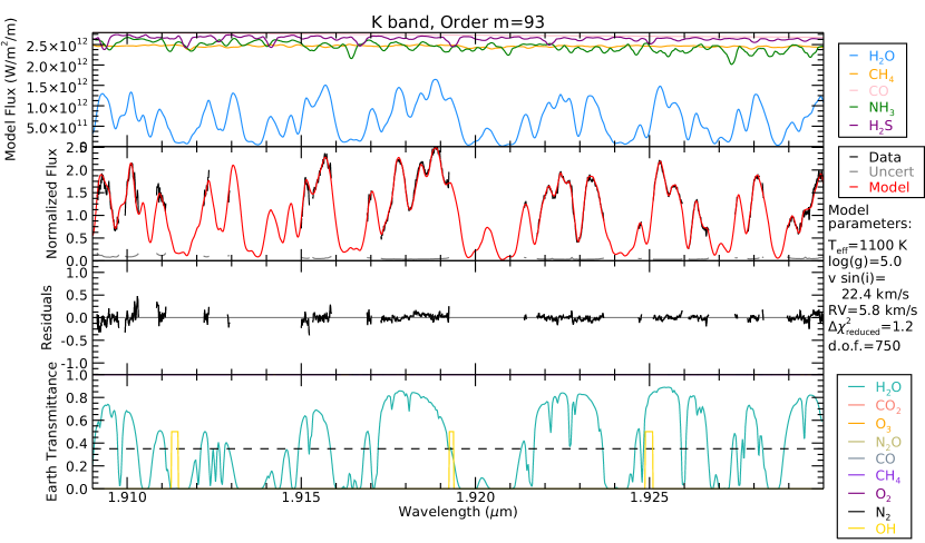
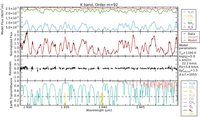
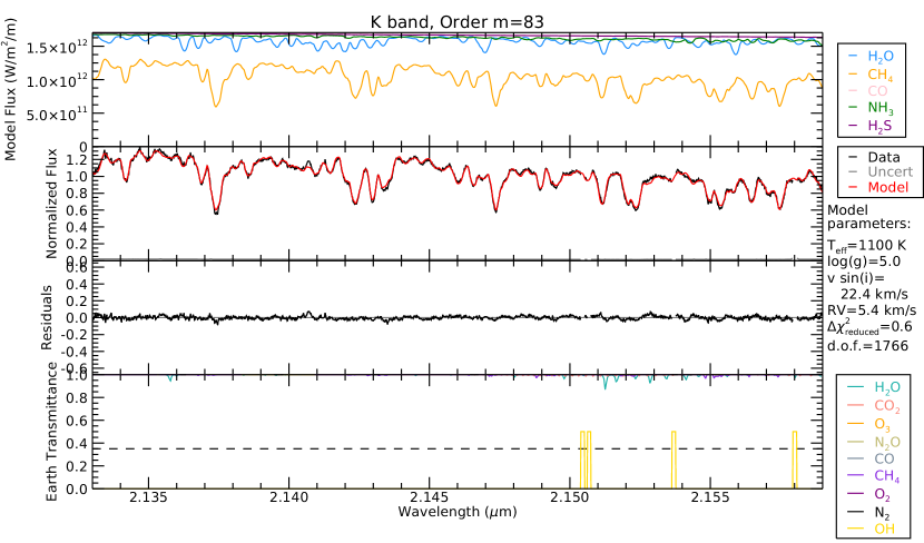
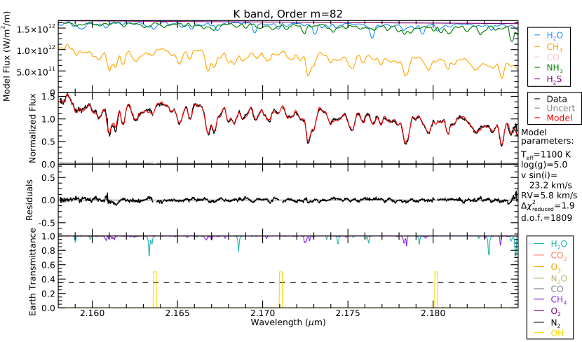
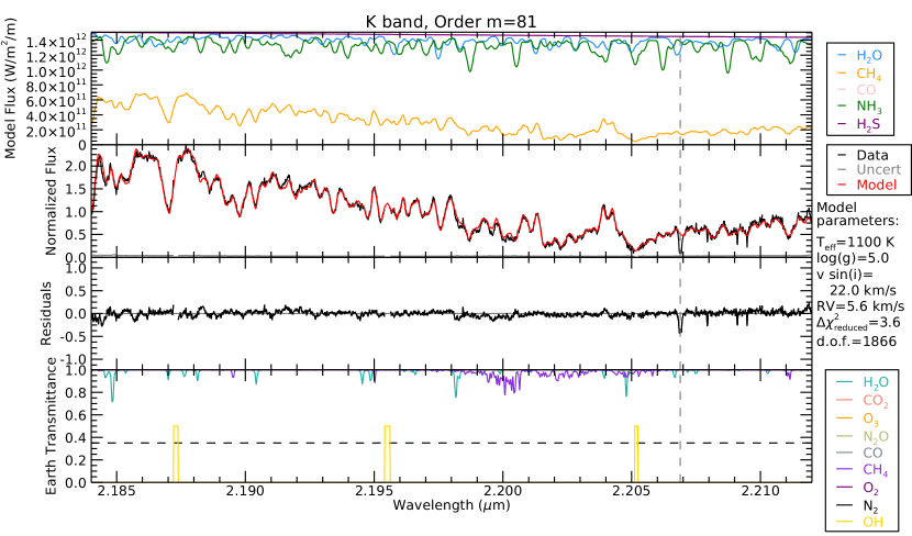
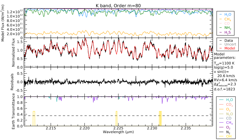
We show the results of the model fitting across all orders for all model families in Fig. 3 and 4. In the top panel, a Bobcat Alternative A model is used to separate the contribution of each molecular species, in order to identify the dominant molecule or molecules in each order. These ‘single-molecule models’ include a single molecule (e.g., water, methane), plus collision-induced absorption from molecular hydrogen and helium. To help identify particular features and molecules, a panel like this is included at the top of almost all of our figures.

We find that the Bobcat Alternative A models with the updated line lists provide the best fits to the data. We adopt the values given by the Bobcat Alternative A models, and present the weighted average of each parameter across all $H$ and $K$ band orders in Table 3. As described in Tannock et al. (2021), we compute the weighted average and the unbiased weighted sample standard deviation, where the weight is $e^{-\chi^{2}_{\rm reduced}}$, so that the better fits and more reliable orders are more heavily weighted. The parameter values given in Fig. 3 and 4 are computed in the same way, but for each order separately. The Bobcat Alternative A models are the most consistent across all orders, and give the smallest uncertainties on the measured parameters. Overall, all models do fairly well in regions dominated by water, while fits are poor in regions dominated by methane.

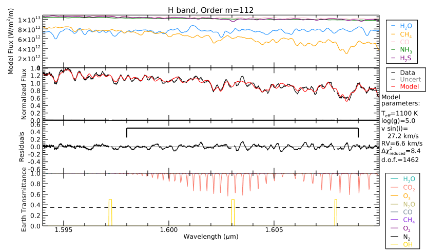
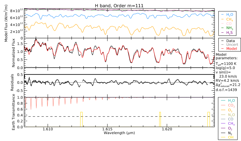
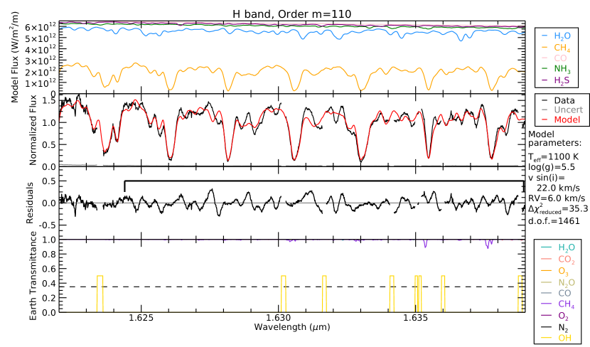
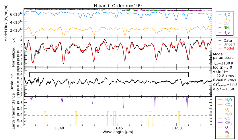
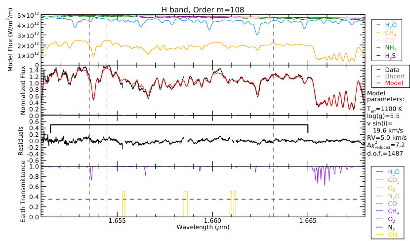
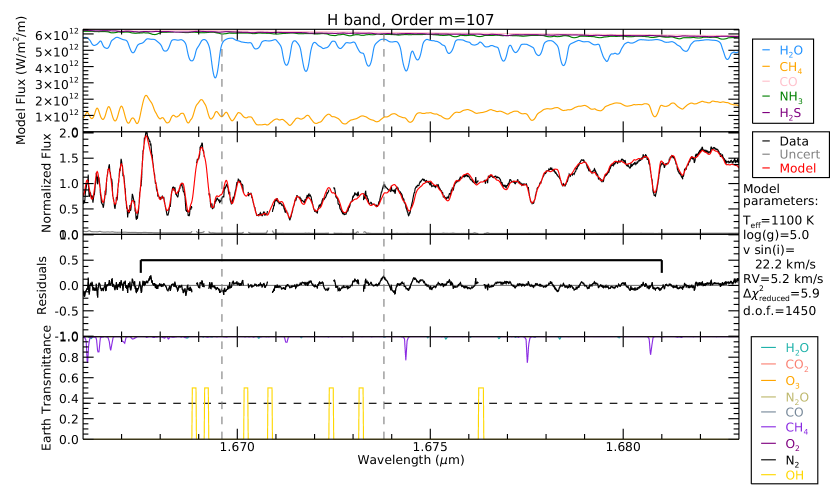
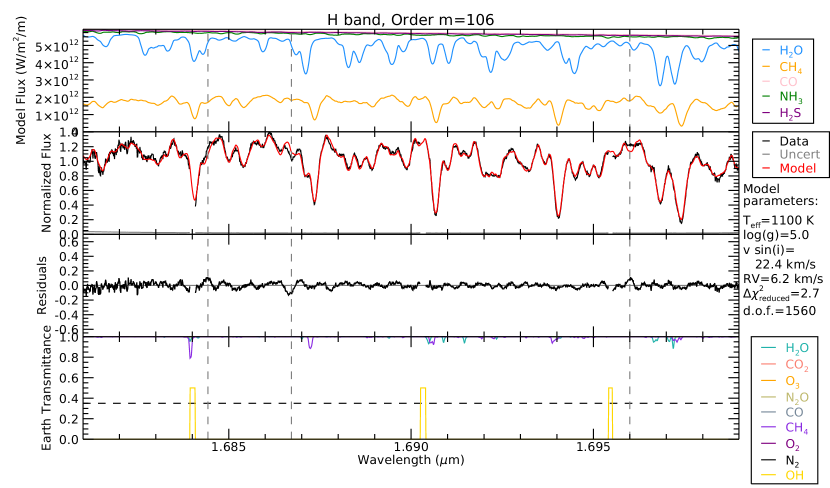
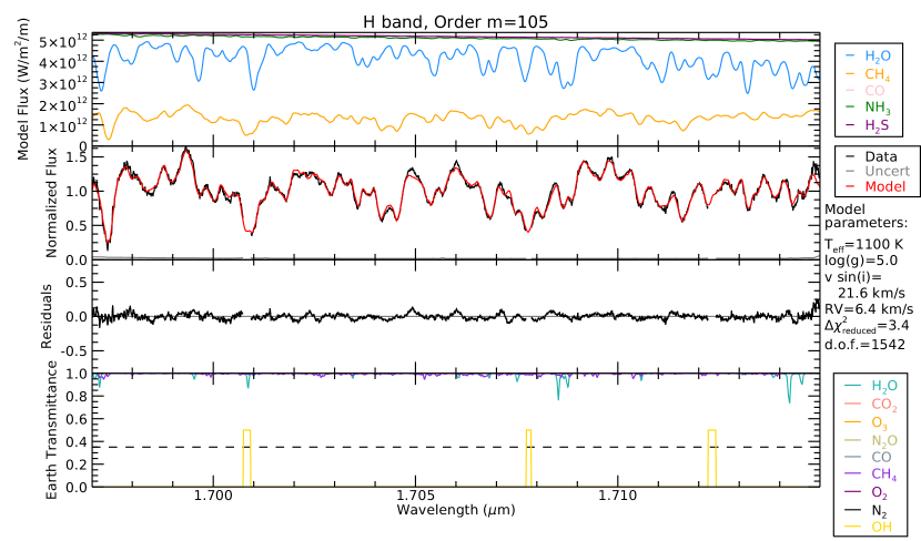
For the remainder of our analysis, we will focus on the results of the Bobcat Alternative A models, unless otherwise stated. We show the best fitting Bobcat Alternative A models for all orders of the $H$ and $K$ bands in Fig. 15 and 28, and in the following sections we highlight a few notable orders and regions.

Table 3: Properties of 2MASS J08173001$-$6155158. Parameters estimated from the spectra presented in this paper are based on all $H$ and $K$ band orders.

Property	Value
Spectral Type	T6
Effective temperature ($T_{\rm eff}$)	1060 $\pm$ 50 K
Surface gravity ($\log{g}$)	5.0 $\pm$ 0.1
Projected rotation velocity ($v\sin{i}$)	22.5 $\pm$ 0.9 km s-1
Radial velocity (RV)	6.1 $\pm$ 0.5 km s-1

Figure 3: Results of the model fitting for the $H$ band. Top panel: The Bobcat Alternative A model spectra of each major molecule with collision-induced absorption from molecular hydrogen and helium included. The Model Flux (the y-axis of the top panel) is what would be measured at the surface of the object. The models shown in this panel have $T_{\rm eff}=1100$ K, $\log{g}=5.0$ (with $g$ in cm s^-2), $v\sin{i}=22.5$ km s^-1, and RV = 6.1 km s^-1, and are also matched to the resolution of the IGRINS data. The IGRINS order numbers ($m$) are given along the top horizontal axis. Second panel from the top: The full $H$-band IGRINS spectrum, with the orders stitched together. Bottom four panels: The parameters of the best-fitting model for each order, from each family of models. From top to bottom the parameters are: RV, $v\sin{i}$, $T_{\rm eff}$, and $\log{g}$. The weighted average of each parameter is given on the right side of the figure. In some cases the best-fitting models are at the maximum and minimum values of the allowed grid, which indicates that these models produce inadequate fits in the particular order. These values are still included in the weighted mean, but have very little weight assigned to them due to their large $\chi^{2}$ statistics.

Figure 4: The same layout as Fig. 3, but for the $K$ band. The $\log{g}$ value is extremely consistent for the Bobcat Alternative A models, with $\log{g}$ = 5.0 in every order of the $K$ band. The standard deviation on this weighted average is therefore zero (see Section 3.2 for details on this calculation). In Table 3 we compute the weighted average and standard deviation based on both the $H$ and $K$ bands, so the standard deviation is non-zero for the final adopted value.

4 Molecule-by-Molecule Analysis of the Model Spectra

In this section we assess the quality of the fits from each family of models. We examine the parameters determined for each region of the spectrum and what the dominant absorbers are in each region. Water (H₂O) and methane (CH₄) are the most abundant absorbers in late-type T dwarf spectra (Burgasser et al., 2006). Carbon monoxide (CO) and ammonia (NH₃) also play a major role, and hydrogen sulfide (H₂S) is the next most abundant absorber. The references for the line lists of the major molecules used in each family of models are listed in Table 4. As 2M0817 is a fairly rapid rotator ($v\sin{i}=22.5\pm 0.9$ km s^-1; Table 3), we see that most lines are in fact blends of the dominant absorbers, most often H₂O and CH₄.

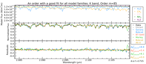
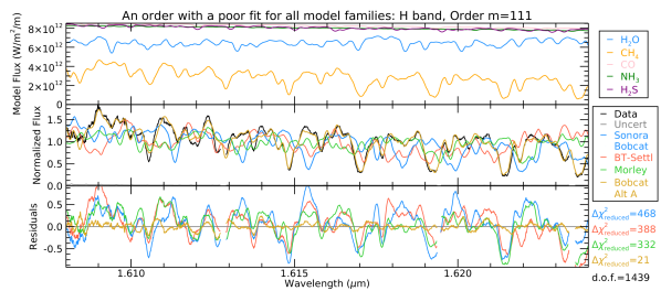
In Fig. 5 we show order $m=85$ of the $K$ band: the order where the models most accurately represent the data. The dominant absorbers in this order are H₂O, and CH₄. The Bobcat Alternative A model provides the best fit, and the residuals for this model are very flat. The other models also do a fair job in matching the major features. For comparison, in Fig. 6, we show order $m=111$ of the $H$ band: one of the orders where all models provide poor fits. The major absorber in this order is CH₄. We see that the locations of the strongest CH₄ features are matched in the Bobcat Alternative A model, which has the most up-to-date CH₄ line list (Table 4). In the following sections, we discuss each molecular absorber separately.

Table 4: Literature references for the line lists for each of the model photosphere families. For information about specific isotopologues, line widths, and how these sources are combined for each family of models please see the original works listed in the column headers.

Molecule	Bobcat Alternative A (Hood et al. in preparation)	Sonora Bobcat (Marley et al., 2021)	Morley (Morley et al., 2012)	BT-Settl (Allard et al., 2012, 2014)
H2O	ExoMol/POKAZATEL (Polyansky et al., 2018); BT2 (Barber et al., 2006)	Tennyson & Yurchenko (2018); BT2 (Barber et al., 2006)	Partridge & Schwenke (1997); HITRAN’08 (Rothman et al., 2009)	BT2 (Barber et al., 2006)
CH4	HITEMP (Hargreaves et al., 2020)	Yurchenko et al. (2013); Exomol/10to10 (Yurchenko & Tennyson, 2014); Spherical Top Data System (Wenger & Champion, 1998)	Spherical Top Data System (Wenger & Champion, 1998); HITRAN’08 (Rothman et al., 2009); Strong et al. (1993)	Spherical Top Data System (Wenger & Champion, 1998)
CO	HITEMP 2010 (Rothman et al., 2010); Li et al. (2015)	HITEMP 2010 (Rothman et al., 2010); Li et al. (2015)	Goorvitch (1994); R. Tipping (1993, private communication); HITRAN’08 (Rothman et al., 2009)	Goorvitch (1994)
NH3	ExoMol/CoYuTe (Coles et al., 2019)	BYTe (Yurchenko et al., 2011)	BYTe (Yurchenko et al., 2011)	Sharp & Burrows (2007)
H2S	ExoMol (Tennyson & Yurchenko, 2012); Azzam et al. (2015); HITRAN 2012 (Rothman et al., 2013)	ExoMol (Tennyson & Yurchenko, 2012); Azzam et al. (2015); HITRAN 2012 (Rothman et al., 2013)	R. Wattson (1996, private communication); HITRAN’08 (Rothman et al., 2009)	HITRAN 2004 (Rothman et al., 2005)

Figure 5: In order $m=85$ of the $K$ band, all models are very well matched to the data. The dominant absorbers in this region are H₂O and CH₄. The top panel shows the Bobcat Alternative A model spectra including opacity from one major molecule at a time, in addition to H₂/He collision-induced absorption. The middle panel shows the IGRINS data (black; uncertainty shown in grey) with the best fitting models from each model family. The Bobcat Alternative A model spectra in the top panel have the same $T_{\rm eff}$ and $\log{g}$ values as the best fitting Bobcat Alternative A model, are broadened to the same $v\sin{i}$, and have the same RV shift applied. The bottom panel shows the residuals (data - model) on the same vertical scale as the middle panel, with the same colour scheme. The data and residuals contain gaps in the plot where strong telluric lines have been masked out. The $\Delta\chi^{2}_{\rm reduced}$ statistic is the difference between the $\chi^{2}_{\rm reduced}$ of the model for the current order and the $\chi^{2}_{\rm reduced}=1.0$ of the best-fitting model (Bobcat Alternative A model) for order $m=85$. The degrees of freedom (d.o.f.) for the $\chi^{2}_{\rm reduced}$ for each model are also shown.

Figure 6: The same layout as Fig. 5, but now showing order $m=111$ of the $H$ band, an order with a poor fit. The dominant absorber in this order is CH₄. The most up-to-date line lists for CH₄ (Hargreaves et al. 2020, used in the Bobcat Alternative A model) provide accurate wavelengths for the deepest lines, but the weaker features in the continuum (likely CH₄ blended with H₂O) are poorly-fit.

4.1 Water

The water-dominated regions of the spectrum provide the most consistent results from fitting models to spectra across all model families (Fig. 3 and 4). The short-wavelength end of the $H$ band (1.454–1.580 $\mu$m) gives consistent results for each model family, and across the various families. The long-wavelength end of the $H$ band (1.750–1.812 $\mu$m) and the short-wavelength end of the $K$ band (1.894–2.100 $\mu$m) give consistent results within each family of models, but not necessarily across the various model families.

We note that the Sonora Bobcat and BT-Settl models give higher estimates of the RV, and there is a trend in RV where the RV increases with wavelength (the models are increasingly blue-shifted) in the short-wavelength end of the $K$ band (1.894–2.060 $\mu$m; Fig. 4) for these two models. NH₃ is also an important absorber in this region but is likely not responsible for this trend in RV because Sonora Bobcat shares the same line lists for ammonia as the Morley models (Yurchenko et al., 2011, BYTe), and the Morley models do not show this trend.

The behaviour for the BT-Settl models indicates that the BT2 (Barber et al., 2006) H₂O line lists, when used alone, are unreliable for RV determinations in this wavelength region. The similar behaviour from Sonora Bobcat indicates that Tennyson & Yurchenko (2018), supplemented with isotopologues from BT2, is also unreliable. The Bobcat Alternative A models use ExoMol/POKAZATEL (Polyansky et al., 2018) as the main H₂O line list, and also use isotopologue data from BT2. However for this model, we obtain very consistent RV measurements in this wavelength region. The improved accuracy of ExoMol/POKAZATEL line lists appear to make up for any discrepancies in BT2. The HITRAN’08 (Rothman et al., 2009) and Partridge & Schwenke (1997) line lists used in the Morley models also give more self-consistent estimates of RV in this region.

Overall we consider water, specifically for the line list used in the Bobcat Alternative A models (ExoMol/POKAZATEL), to be the most reliable molecule for determining the physical parameters of cold brown dwarfs, producing values that we trust.

4.2 Methane

As seen in Fig. 3 and 4, there is much greater variation in the parameters estimated in the methane-dominated regions (1.60–1.73 $\mu$m in the $H$ band and 2.11–2.40 $\mu$m in the $K$ band) compared to the water-dominated regions, and the $v\sin{i}$ values are particularly discrepant. Each family of models uses a different set of line lists for CH₄, though there is some overlap between the Sonora Bobcat, Morley, and BT-Settl models which use multiple sources for their CH₄ line lists (Table 4). Uncertainty has been reported for theoretical CH₄ band positions previously: Canty et al. (2015) report offsets between the absorption features in their observed data and the peaks of CH₄ opacity from the Exomol/10to10 line list (Yurchenko & Tennyson, 2014) between 1.615 and 1.710 $\mu$m.

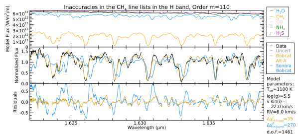
In Fig. 7 we show a Sonora Bobcat model and a Bobcat Alternative A model with identical physical parameters for an order in the methane region of the $H$ band (order $m=111$ of the $H$ band, 1.608–1.624 $\mu$m). The CH₄ lines used in the Sonora Bobcat models (the same as examined by Canty et al. 2015; Table 4) do not match the data well, and appear to have a stretch across this order. Both models poorly fit the weaker lines and the continuum in this region. Radial velocities estimated by the Sonora Bobcat models are discrepant in the methane-dominated regions, due to these inaccurate line positions. We find significant improvement from the line lists used in the Bobcat Alternative A models (HITEMP, Hargreaves et al. 2020) over older models in regions dominated by CH₄, in particular in the $H$ band. However, the regions dominated by CH₄, even in the Bobcat Alternative A models, still have the most variation in the estimates of the physical parameters. We summarize these regions in Table 5, noted as ‘CH₄ regions.’ Models using older CH₄ line lists should therefore be used with caution. Unaccounted for disequilibrium chemistry may impact these weaker features. We do not explore disequilibrium chemistry for CH₄ or H₂O in this work, but see Section 4.3 for details on CO disequilibrium chemistry.

Recent theoretical line lists are far more complete than the previously-used laboratory-measured line lists, which are designed to have very accurate line positions but capture fewer lines due to the limits on resolution in laboratory experiments. Therefore, theoretical line lists should improve accuracy in regions of the spectrum with weaker bands present, if those bands were unresolved in the laboratory lists. A recent improvement in the available line lists has been the combinations of theoretical line lists with laboratory measurements (e.g., HITEMP, Hargreaves et al. 2020). Such combination lists provide the best of both worlds, as we show here, where we find a dramatic improvement to high resolution spectroscopic fits.

Figure 7: The improvement made with the newer CH₄ line lists is most apparent in order $m=110$ of the $H$ band. The top panel is the same as Fig. 5: the Bobcat Alternative A model spectra of each major molecule with H₂/He collision-induced absorption are shown. Here the middle panel shows the IGRINS data (black), the Sonora Bobcat model (light blue), and the Bobcat Alternative A model (gold). The models have identical physical parameters, rotational broadening ($v\sin{i}$), and RV shift. The bottom panel shows the residuals (data - model) on the same vertical scale, with the same colour scheme. The deepest features are CH₄, and the weaker features in the continuum are mainly CH₄ or CH₄ blended with H₂O. The Bobcat Alternative A model shows excellent agreement with the data in the major features, while the Sonora Bobcat model appears to have a stretch causing misalignment in the major features when compared to the IGRINS data.

4.3 Carbon Monoxide

For effective temperatures $\lesssim$ 1300 K (near the L/T transition), the dominant carbon-bearing molecule in the visible part of atmospheres of brown dwarfs switches from CO to CH₄ (Fegley & Lodders, 1996; Burrows et al., 1997). There are still signatures of CO in the spectra of cold brown dwarfs, and carbon exists abundantly as CO deeper in the atmosphere, where temperatures are higher.

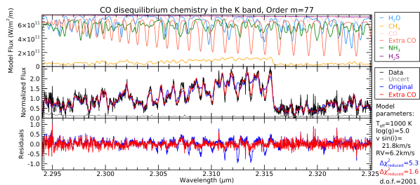
We found that at the CO bands our model fitting selected higher effective temperatures ($T_{\rm eff}\sim$ 1200 K) compared to other orders. Accordingly, we observed several notable features in the residuals of orders $m=77$ through $m=73$ of the $K$ band (2.294–2.445 $\mu$m), as well as in order $m=115$ of the $H$ band (1.554–1.569 $\mu$m), where a CO band head is present. The features in the residuals aligned with CO absorption features. We show an example of this in Fig. 8, along with a model with increased CO abundance, providing an improved fit. The model with increased CO abundance is also shown in Fig. 3, 4, and the Appendix figures, and is described in detail below.

This increased CO abundance implies disequilibrium chemistry, which can occur when vertical mixing occurs in the atmosphere (Lodders & Fegley, 2002; Saumon et al., 2003). If CO is being brought from deeper, hotter layers to the upper atmosphere faster than the chemical reaction that converts CO to CH₄, there will be more CO in the upper layers of the atmosphere than predicted from chemical equilibrium.

The Sonora Bobcat and Bobcat Alternative A models use the same cloudless, rainout chemical equilibrium structure models (Marley et al., 2021). These structure models assume chemical equilibrium and give the pressure, temperature, and chemical abundances throughout the atmosphere. To improve our fitting, we generated a small grid of Bobcat Alternative A models with varied amounts of CO, deviating from the chemical equilibrium assumptions used in the Sonora Bobcat structure models. We took a simple approach where we fixed the volume mixing ratio (VMR) for CO to values of $10^{-6}$, $3\times 10^{-5}$, $10^{-5}$, $3\times 10^{-4}$, $10^{-4}$, $3\times 10^{-3}$, and $10^{-3}$. This is a zeroth-order approximation, as 1) the CO VMR is not constant throughout the entire atmosphere, 2) other abundances like CH₄ and H₂O will also be affected by disequilibrium chemistry, and 3) we are using the temperature-pressure profile from the chemical equilibrium Sonora Bobcat models, but a much higher CO abundance could affect the temperature-pressure profile.

We found a CO VMR of $3\times 10^{-4}$ provided the best fits to our data. Fig. 8 shows a comparison of the original equilibrium chemistry model to the model with this fixed CO VMR value (Fig. 3, 4, and the Appendix figures also show models with this fixed CO VMR). In equilibrium models, the CO VMR ranges from $10^{-7}$ to $2.5\times 10^{-4}$ for pressures probed by the $K$ band. The CO VMR value of the best fitting model is slightly higher than the range in values expected for equilibrium, and explains why our initial fitting selected models with higher effective temperatures, as the CO abundance would be higher in the hotter models.

Following the method in Section 6.1 of Miles et al. (2020), we use the quench pressure to estimate the eddy diffusion coefficient ($\log{K_{zz}}$, where $K_{zz}$ has units of cm² s^-1). We find $\log{K_{zz}=6.4}$ for 2M0817. This value is in line with the range of relatively low inferred $K_{zz}$ values ($\sim$100 $\times$ lower than expected from mixing length theory of convection) from Miles et al. (2020) for colder ($T_{\rm eff}\leq 750$ K) brown dwarfs. Miles et al. attribute the low $K_{zz}$ values to quenching in radiative regions of the atmosphere, where mixing is likely more sluggish than in convective regions. Interestingly, we find the same behaviour here at $\sim$ 300 K hotter $T_{\rm eff}$. The Sonora model pressure-temperature profile is completely radiative down past the quench pressure of 20 bars, to a pressure of 30 bars, where the atmosphere transitions to the deep convective region.

Disequilibrium chemistry for CO has been observed spectroscopically and inferred photometrically in many other late-type T dwarfs and Y dwarfs (e.g., Noll et al. 1997; Oppenheimer et al. 1998; Golimowski et al. 2004; Geballe et al. 2009; Leggett et al. 2012; Sorahana & Yamamura 2012; Miles et al. 2020), and has been known in Jupiter for decades (Prinn & Barshay, 1977; Noll et al., 1988). The growing number of T and Y dwarfs with evidence for CO disequilibrium chemistry indicates that vertical mixing is an important factor in accurately modelling brown dwarf spectra even at cold temperatures.

Figure 8: Order $m=77$ of the $K$ band is dominated by CH₄, but CO and H₂O are also important absorbers. Here the top panel is similar to Fig. 5, with an extra line for a model with an increased CO abundance (CO volume mixing ratio of $3\times 10^{-4}$, labelled ‘Extra CO’). The middle panel shows the observed spectrum with two versions of a Bobcat Alternative A model, one with the CO as estimated by chemical equilibrium (labelled ‘Original’) and one with an increased abundance of CO (labelled ‘Extra CO’). The bottom panel shows the residuals for the two models. The CO strength in particular is important to improve the accuracy of the models in the long end of the $K$ band. It is clear that the depth of the features in the ‘Original’ model is too weak at the positions of the CO features, implying that vertical mixing must be taking place in this atmosphere.

4.4 Ammonia

Water and methane are the dominant absorbers in the spectra of late-type T dwarfs, but ammonia is important too, especially at T$<$700 K (the coldest T dwarfs and Y dwarfs), where it becomes the dominant nitrogen-bearing molecule (Lodders & Fegley, 2002). Ammonia is of special significance as it is the defining species in the spectra of Y dwarfs (Cushing et al., 2011).

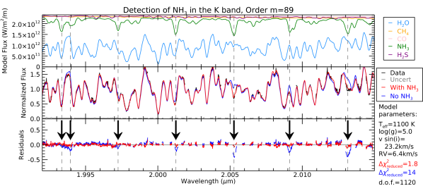
The choice of an ammonia line list (among published lists) does not appear to significantly impact the physical parameters derived by comparing to models, but ammonia lines are clearly present in the observed spectrum and are important to include in the models. We are able to detect ammonia clearly in several regions of our spectrum.

This T6 dwarf joins the handful of T dwarfs with confirmed NH₃ detections in the near-infrared. Saumon et al. (2000) find evidence for NH₃ in the $H$- and $K$-band spectra of Gliese 229B (spectral type T6.5p, $T_{\rm eff}\sim 950$ K) and Canty et al. (2015) report the detection of several NH₃ absorption features in the $H$ and $K$ bands in a T8 and T9 dwarf. Bochanski et al. (2011) additionally report detections of NH₃ in a T9 dwarf, however, Saumon et al. (2012) question whether some of those detections are indeed attributable to NH₃. Saumon et al. (2012) do confirm the stronger NH₃ features at $\sim$2 $\mu$m in the spectrum of Bochanski et al. (2011). We re-confirm the strongest NH₃ identified in these works, but some of the weaker lines identified in these later spectral types do not appear in our warmer T6 dwarf.

Cushing et al. (2021) indicate NH₃ features should be present in the infrared at 1.03, 1.21, 1.31, 1.51, 1.66, 1.98, and 2.26 $\mu$m, but would be blended with stronger H₂O and CH₄ lines making them difficult to detect. While the features at 1.03, 1.21, and 1.31 $\mu$m are outside of our wavelength coverage, we do have clear detections of NH₃ at 1.51, 1.98, and 2.26 $\mu$m using the Bobcat Alternative A models. The ammonia lines in our observed spectra are indeed blended with stronger H₂O lines, but we are able to detect them nonetheless. We compared Bobcat Alternative A models, with and without NH₃, and the presence of the NH₃ is clear in the comb-like residuals of Fig. 9. We also see significant improvement in the reduced $\chi^{2}$ statistic when NH₃ is included in the model. We find that the NH₃ at 1.66 $\mu$m is far too weak to detect amongst the much stronger H₂O and CH₄ features in this region for an object of this temperature. While NH₃ has been detected in early T dwarfs in the mid-infrared (Roellig et al., 2004; Cushing et al., 2006), 2M0817 is the warmest brown dwarf with individual NH₃ lines detected in the near-infrared.

More recently, Line et al. (2015); Line et al. (2017) and Zalesky et al. (2019) constrained the NH₃ abundance for multiple cold brown dwarfs (spectral types T7 and later, including several Y dwarfs) with low-resolution ($R<300$ with IRTF/SpeX and HST/WFC3) retrievals. These studies are sensitive to how NH₃ opacities influence the spectroscopic appearance of cold brown dwarfs, but the low-resolution of the observations prevents identification of individual NH₃ lines in the spectra.

Figure 9: The same layout as Fig. 8, but showing Bobcat Alternative A models with and without NH₃. Arrows indicate where the model without NH₃ deviates from the data. The NH₃ lines are blended with stronger H₂O lines, but we see significant improvement in the $\chi^{2}_{\rm reduced}$ values when NH₃ is included in the model. Order $m=89$ of the $K$ band has many strong telluric lines, but is still well fit by the models. It is difficult to discern the data from the model containing NH₃, and the quality of the fit is reflect in the flat residuals and low $\chi^{2}_{\rm reduced}$ value.

4.5 Hydrogen Sulfide

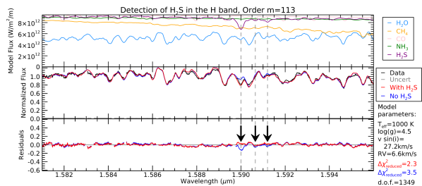
We present clear, unambiguous detections of H₂S in 2M0817. Our most notable detection is a feature at 1.5900 $\mu$m. This feature is blended with a weak H₂O line at the same position, so we show our data compared to Bobcat Alternative A models with and without H₂S in Fig. 10. We see the clear signature of this H₂S line in the residuals, as well as the presence of other weaker H₂S lines nearby at 1.5906 $\mu$m and 1.5912 $\mu$m.

There is only one other report of a possible H₂S detection in a brown dwarf in the literature. Saumon et al. (2000) note an H₂S absorption feature at 2.1084 $\mu$m in the spectrum of Gliese 229B (spectral type T6.5p). However, we do not confirm this line in our data, nor do our updated models predict any H₂S lines at this position.

H₂S has been identified in the giant planets of our Solar System: Irwin et al. (2018) detect H₂S in the atmosphere of Uranus and Irwin et al. (2019) present a tentative detection of H₂S in Neptune, both in the 1.57–1.59 $\mu$m region, the same region in which we have our clearest detection. Detections of H₂S in Jupiter have also been debated (Noll et al., 1995; Niemann et al., 1998). Our spectrum of 2M0817 exhibits the only convincing detection of H₂S in an extra-solar atmosphere to date.

We estimated the column density of H₂S ($N_{\rm H_{2}S}$) in the atmosphere of 2M0817 to compare against the Irwin et al. (2018, 2019) estimates for Uranus and Neptune. We first determined the pressure ($P$) corresponding to the brightness temperature ($T_{b}$) at the centre of the strongest H₂S line in the Bobcat Alternative A model spectrum ($P=14$ bars and $T_{b}=1420$ K). Then, for each layer in the model atmosphere, we calculated the local number density of all gas molecules using the ideal gas law. We obtained the local number density of H₂S specifically by multiplying with the H₂S VMR (H₂S has an approximately constant equilibrium VMR of of $2.5\times 10^{-5}$ throughout the Bobcat Alternative A model atmosphere). Integrating this H₂S number density from the pressure of the absorbing layer to the top of the atmosphere gives us the column density of H₂S, $N_{\rm H_{2}S}\sim 7.7\times 10^{20}$ cm^-2. This value is 3 to 130 times higher than column amounts determined from retrievals for solar system planets: $N_{\rm H_{2}S}$ varies between $6\times 10^{18}$ to $4.9\times 10^{19}$ molecules per cm² across the disc of Uranus (Irwin et al., 2018), and $9\times 10^{18}$ to $2.8\times 10^{20}$ molecules per cm² across the disc of Neptune (Irwin et al., 2019).

The detection of H₂S also offers tentative evidence of iron rain-out in the atmosphere of 2M0817. Below temperatures of 2300 K, iron is predominantly in the form of metallic droplets that settle to deeper atmospheric layers (Fegley & Lodders, 1994; Burrows & Sharp, 1999). At temperatures $\lesssim$ 750 K, any iron in the atmosphere would take the form of FeS, leaving no sulphur to form H₂S, meaning that H₂S would be absent from spectra (Fegley & Lodders, 1994; Burrows et al., 2001; Lodders & Fegley, 2006). The surface chemical reactions for the conversion of FeS to solid iron and H₂S are described in Helling et al. (2019). We detect H₂S in the atmosphere of 2M0817, so iron must be in the process of raining out. Rain-out chemistry is indeed assumed in the Sonora Bobcat and Bobcat Alternative A models.

Figure 10: The same layout as Fig. 9, but showing Bobcat Alternative A models with and without H₂S. This order shows a clear H₂S detection at 1.5900 $\mu$m. Order $m=113$ of the $H$ band is well fit by models. The H₂S line of interest is blended with an H₂O line, but we see the impact of H₂S in the residuals, and improvement in the $\chi^{2}_{\rm reduced}$ value for the model including H₂S.

4.6 Molecular Hydrogen

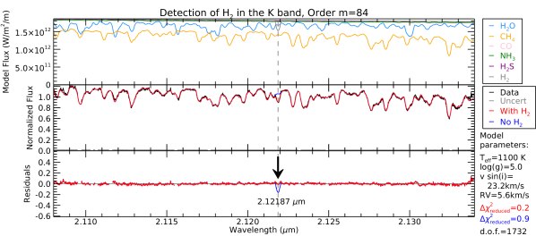
In order $m=84$ of the $K$ band, we identified an absorption feature at 2.12187 $\mu$m that does not appear in any model of any family. This line is indicated by a black arrow in Fig. 11. We first identified this line through our model deviation analysis (Sec. 4.7), and after correcting for 2M0817’s radial velocity (6.1 $\pm$ 0.5 km/s, Table 3), we found the position of this line to be 2.12183 $\pm$ 0.00005 $\mu$m (vacuum wavelength). This matches the 2.121834 $\mu$m wavelength of the molecular hydrogen (H₂) 1-0 S(1) transition to six significant figures (Scoville et al., 1983; Roueff et al., 2019). The H₂ 1-0 S(1) feature is among the strongest H₂ lines when present in emission in photon-dominated regions, shocks, planetary nebulae, young stellar objects, and starburst galaxies (e.g., Habart et al. 2005). It has never before been detected in absorption in an extra-solar atmosphere, although it has been seen in Jupiter, Saturn, and Neptune (Kim et al., 1995; Trafton et al., 1997).

We added the HITRAN 2016 (Gordon et al., 2017) line list for H₂ to the Bobcat Alternative A model and found excellent agreement between order $m=84$ of our observed spectrum and the model. As we did for our NH₃ and H₂S identification, we present models with and without H₂ in Fig. 11, and we see the clear signature of the H₂ line in the residuals. We investigated each of the other wavelength regions where the model showed strong H₂ absorption features, in particular the 1-0 S(3) transition (1.957559 $\mu$m), the 1-0 S(2) transition (2.033758 $\mu$m), and the strongest line of the $Q$-branch: the 1-0 Q(1) transition (2.406592 $\mu$m; Gautier et al. 1976; Roueff et al. 2019). We were unable to detect additional H₂ features, due to either the much stronger absorption by other molecules (mostly CH₄), the lower SNR in other parts of the spectrum, or both.

The first detection of a molecular hydrogen absorption feature in a brown dwarf atmosphere gives a new semi-empirical upper limit on the atmospheric dust concentration in this T6 dwarf. We attain this limit by comparing to the concentration content of the interstellar medium (ISM), where an atomic hydrogen column density of $N_{\text{H\,{i}}}=2.2\times 10^{21}$ cm^-2 corresponds to a visual extinction of $A_{V}=1.0$ mag, given a 100:1 gas-to-dust ratio (Gorenstein, 1975). We expect the ISM gas-to-dust ratio to be orders of magnitude lower than in the upper atmosphere of this brown dwarf, which unlike the ISM is gravitationally differentiated. Silicates (e.g., SiO₃, MgSiO₃, Mg₂SiO₄) have $\sim$38–70 times higher molecular weights than molecular hydrogen, and should have settled mostly below the H₂-dominated layers of the atmosphere.

The $K$-band extinction in the ISM is such that $A_{K}/A_{V}=0.114$ (Table 3 of Cardelli et al., 1989), so in the ISM $N_{\text{H\,{i}}}/A_{K}=1.94\times 10^{22}$ cm^-2 mag^-1. Virtually all of the hydrogen in the brown dwarf atmosphere is expected to be bound in H₂ (e.g, Burrows et al. 2001), so the projected H₂ column density per magnitude of ISM-like $K$-band extinction is $N_{\rm H_{2}}/A_{K}=0.97\times 10^{22}$ cm^-2 mag^-1.

Following the same prescription as for our calculation of the H₂S column density (Section 4.5), we obtain that the H₂ column density in the visible atmosphere of 2M0817 is $N_{\rm H_{2}}\sim 5.1\times 10^{24}$ cm^-2 (the centre of the strongest line corresponds to $P=4$ bars and $T_{b}=1070$ K, and H₂ has an approximately constant equilibrium VMR of 0.836 throughout the Bobcat Alternative A model atmosphere). If the gas-to-dust ratio in the atmosphere of 2M0817 were ISM-like, this H₂ column density would correspond to $A_{K}\sim 500$ mag of extinction. Instead, the H₂ line is readily detectable, so $A_{K}$ must be less than 1 mag. This implies that the amount of dust in the atmosphere is $>$500 times less than the interstellar value, and that the atmosphere of 2M018 is almost completely dust-free, as expected for a late-T dwarf.

Finally, the presence of the H₂ line in absorption instead of in emission indicates that the H₂ layer is cooler than the layers underneath it. Hence, the upper atmosphere of 2M0817 does not have a strong thermal inversion, as might otherwise be expected in the presence of hot eddies (Showman et al., 2020).

Figure 11: The same layout as Fig. 9, but showing Bobcat Alternative A models with and without H₂ absorption (collision-induced absorption from molecular hydrogen and helium is included in both models). This order shows a clear H₂ absorption feature at 2.12187 $\mu$m, indicated with a black arrow. Order $m=84$ of the $K$ band is very well fit by models, and we see significant improvement in the $\chi^{2}_{\rm reduced}$ value for the model including H₂ absorption.

4.7 Shortcomings of the Models and Unidentified Lines

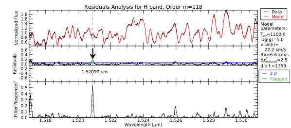
A goal of this work is to identify regions where the photospheric models do not completely reproduce the features in the observed spectra. To identify regions and specific absorption lines in the data which are not well reproduced with the models, we performed two checks. First, we measured the standard deviation, $\sigma$, of the residuals in each order, and then selected regions with at least five consecutive pixels more than $2\sigma$ away from zero. Second, we applied a matched filter to the residuals by convolving the residuals with a template of an inverted absorption feature. For each order, we selected a telluric absorption feature in the reduced A0 V standard’s spectrum to use as our filter template. We selected features surrounded by a flat continuum and avoided lines with greater than 65 per cent absorption (the threshold for our continuum mask, Section 2.1). In orders which had very few, or very weak telluric features, we selected a line from a neighbouring order. We then identified regions in the spectra where both the pixel values were outside of two standard deviations, and the matched filter response was higher than the surrounding pixels. This helped to eliminate false detections due to noise. We performed these checks only for the Bobcat Alternative A models, as they are the most up-to-date and provide the best fits to the data. We show an example of this analysis in Fig. 12, and we summarize the regions of interest in Table 5, with a brief description of the potential issue affecting the model in each case. These discrepancies can be seen in Fig. 15 and 28, indicated with with vertical grey dashed lines for individual features, and black brackets for wider discrepant regions. The H₂ feature (Section 4.6) was initially identified through this type of analysis.

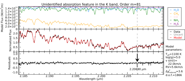
Most notably, a line is clearly missing from the models at 2.20695 $\mu$m in order $m=81$ of the $K$ band, shown in Fig. 13. None of the models includes a line at this wavelength, and we have not identified the element or molecule responsible for this feature. Additionally, we find no absorption or emission in the A0 V stars at the wavelengths given in Table 5 which could introduce these unidentified features to our T6 spectrum. The feature in $H$ band order $m$=121 does line up with a weak telluric H₂O feature, but given the difference in the line widths, we believe this discrepancy between the data and model is not caused by the telluric line.

The Bobcat Alternative A models we use to anlayze our data are comprised of the five most abundant molecules (H₂O, CH₄, CO, NH₃, and H₂S), plus collision-induced absorption from molecular hydrogen and helium. The Sonora Bobcat, Morley, and BT-Settl models consist of more complete sets of molecules. We have confirmed that the lines listed in Table 5 are indeed missing in all families of models. We cannot eliminate all molecules that are included in the more complete Sonora Bobcat, Morley, and BT-Settl model families as being responsible for these missing lines, as the line lists could be incomplete or inaccurate, or there could be disequilibrium chemistry taking place, as we observed with CO (Section 4.3). We also confirmed that H₂ is not responsible for any of the unidentified lines.

Disequilibrium chemistry could imply that other mixing-sensitive gases such as phosphine (PH₃; the next most abundant molecule in these cold atmospheres) could also be present at higher abundances than expected for chemical equilibrium (Fegley & Lodders, 1996). We generated a Bobcat Alternative A model with a greatly over-estimated abundance of PH₃ (VMR of $1\times 10^{-4}$, which is more than 300 times the amount expected for equilibrium chemistry, and would require far more phosphorus than would be available in a solar-composition atmosphere) to compare to our spectra, intending to match the locations of the PH₃ features to the unidentified lines. We use the SAlTY line list from Exomol (Sousa-Silva et al., 2015) for PH₃. We found that the PH₃ features did not match with any of the unidentified lines, and PH₃ is likely not responsible for these features. A study by Miles et al. (2020) searched for PH₃ in atmospheres of cold brown dwarfs displaying disequilibrium CO absorption. This study was performed in the $L$ and $M$ bands (centred at 3.45 $\mu$m and 4.75 $\mu$m, respectively), where H₂O, CH₄, and NH₃ absorb less strongly, but PH₃ absorbs much more strongly, and so should give the best chance at detecting PH₃. Unfortunately, they were also unable to detect PH₃.

Among the list of unidentified lines in Table 5, we list nearly the full wavelength coverage of orders $m=113$ through $m=107$ of the $H$ band. These orders cover 1.596–1.681 $\mu$m and the dominant absorber in these orders is CH₄. As discussed in Section 4.2, while the strongest absorption features are very well modelled in the Bobcat Alternative A models, the weaker features and continua in the models deviate significantly from the observations. We observe some bumpiness in the residuals throughout the entire IGRINS wavelength coverage, especially in these CH₄-dominant regions of the $H$-band. There are a host of weaker features that are not being taken into account in the models, and these features contribute a non-trivial amount to the atmospheric opacity.

Figure 12: An example of the analysis done on the residuals to identify discrepancies between the models and data. The top panel shows the IGRINS spectrum with the best-fitting Bobcat Alternative A model for this order. The middle panel shows the residuals on the same y-scale as the top panel. Horizontal blue lines delineate $2\sigma$ threshold, and regions with more than five consecutive pixels beyond $2\sigma$ are highlighted with green. The filter response of a matched filter using a clean telluric line surrounded by a flat continuum is shown in the bottom panel. There is a clear outlier region at 1.52094 $\mu$m flagged by both the residuals analysis, and also giving a high filter response. Other regions with a high filter response (e.g., 1.51714 $\mu$m and 1.52602 $\mu$m) don’t meet our residuals criteria, and are therefore more likely due to noise in the data. The dominant absorber in order $m=118$ of the $H$ band is H₂O, which also appears to be the molecule responsible for the flagged feature.

Figure 13: The same layout as Fig. 11, but showing the best-fitting Bobcat Alternative A model for this order. Order $m=81$ of the $K$ band is fit well by models, and shows an unknown absorption feature that doesn’t appear in any model of any family at 2.20690 $\mu$m. This line is indicated with a black arrow.

Table 5: The wavelengths of discrepancies in the models and unidentified absorption features. These regions are identified in Fig. 15 and 28, with vertical grey dashed lines for individual features, and black brackets for regions.

Band	Order	Wavelength	Notes
	($m$)	($\mu$m)
$H$	121	1.48463	Potential issue with blended line or something missing in the model
$H$	118	1.52090	A line appears in the model which is missing in the data (see Fig. 12). The model line appears to be a water/ammonia blend.
$H$	116	1.55120	Potential issue with blended line (H2O and NH3?)
$H$	115	1.56396	Potential issue with blended line (H2O and NH3 or H2O and H2S?)
$H$	113	1.5875–1.5960	CH4 region
$H$	112	1.5980–1.6090	CH4 region
$H$	111	1.6080–1.6240	CH4 region
$H$	110	1.6244–1.6390	CH4 region
$H$	109	1.6375–1.6510	CH4 region
$H$	108	1.6515–1.6650	CH4 region
$H$	108	1.65355	Potential issue with blended line (CH4 and H2O?)
$H$	108	1.65446	Model over-estimates flux
$H$	108	1.66319	Model over-estimates flux
$H$	107	1.6675–1.6810	CH4 region
$H$	107	1.66960	Line too weak in model
$H$	107	1.67380	Model under-estimates flux
$H$	106	1.68443	Potential issue with blended line (CH4 and H2O?)
$H$	106	1.68672	Potential issue with blended line (CH4 and H2O?)
$H$	106	1.69600	Potential issue with blended line (CH4 and H2O?)
$K$	87	2.04020	Model over-estimates flux
$K$	87	2.05478	Model under-estimates flux
$K$	81	2.20690	Line missing from model (see Fig. 13)

5 Lessons Learned

We find that atmospheric models that use state-of-the-art line lists represent observations well. We are now able to extract more precise information from our data than merely detect the most abundant molecules: we can detect absorption by trace species that have never been seen before (like H₂S and H₂), see low abundance species, and more readily detect abundances of species (as we have done for CO here).

In all cases we recommend using the most-up-to-date models available with the most recent molecular line lists. We have found that the line lists used in the Bobcat Alternative A models (Table 4) give the most reliable and consistent estimates of all physical parameters across all wavelength regions of this study. More generally, we have found that all models do an adequate job fitting the data in regions where H₂O is the dominant absorber.

We summarize our main recommendations and warnings, organized by the information of interest in the following two subsections.

5.1 Fitted Spectroscopic Parameters

Effective Temperature ($T_{\rm eff}$) measurements are most accurate and consistent in the $K$ band, in regions where H₂O is the dominant opacity source. We recommend using the Bobcat Alternative A models for measuring $T_{\rm eff}$ anywhere in the $H$ and $K$ bands. The Morley models over-estimate $T_{\rm eff}$ in the $H$ band and the Sonora Bobcat models over-estimate $T_{\rm eff}$ in the $K$ band, while The BT-Settl models under-estimate $T_{\rm eff}$ in the $K$ band. If disequilibrium chemistry effects are not taken into consideration, $T_{\rm eff}$ may also be over-estimated.

Surface Gravity ($\log{g}$) measurements are the most accurate and consistent in regions where H₂O is the dominant opacity source in the $H$ band. We recommend using the Bobcat Alternative A models for measuring $\log{g}$ anywhere in the $H$ and $K$ bands. The Sonora Bobcat models over-estimate $\log{g}$ in the $K$ band. $\log{g}$ may also be over estimated in regions where the dominant molecule switches from H₂O to CH₄, near the peaks of $H$ and $K$ bands (1.6 $\mu$m and 2.1 $\mu$m, respectively).

Projected Rotation Velocity ($v\sin{i}$) measurements are the most accurate and consistent in regions where H₂O is the dominant opacity source in both the $H$ and $K$ bands. We recommend using the Bobcat Alternative A models for measuring $v\sin{i}$ anywhere in the $H$ and $K$ bands. We recommend using the region from 1.45 to 1.57 $\mu$m in the $H$ band, or 1.89 to 2.10 $\mu$m in the $K$ band if measuring $v\sin{i}$ with any other model. $v\sin{i}$ may be over estimated in regions where the dominant molecule switches from H₂O to CH₄, near the peaks of $H$ and $K$ bands (1.6 $\mu$m and 2.1 $\mu$m, respectively).

Radial Velocity (RV) measurements are the most accurate and consistent in regions where H₂O is the dominant opacity source in both the $H$ and $K$ bands. We recommend using the Bobcat Alternative A models for measuring RV anywhere in the $H$ and $K$ bands. We recommend using the region from 1.45 to 1.58 $\mu$m in the $H$ band if measuring RV with any other model. RV measurements demonstrate a blueshift with wavelength when measured from the Sonora Bobcat and BT-Settl models between 1.894 and 2.060 $\mu$m.

5.2 Specific Molecules

Water (H₂O) is the dominant opacity source between 1.45 and 1.58 $\mu$m in the $H$ band, and between 1.89 and 2.10 $\mu$m in the $K$ band. The H₂O-dominant region of the $H$ band (1.45–1.58 $\mu$m) gives consistent results for all parameters across all model families. We recommend using the ExoMol/POKAZATEL (Polyansky et al., 2018) line list when studying water.

Methane (CH₄) is the dominant opacity source between 1.60 and 1.73 $\mu$m in the $H$ band, and between 2.10 and 2.48 $\mu$m in the $K$ band. The CH₄-dominant region of the $K$ band (2.10–2.48 $\mu$m) gives consistent results for all parameters for the Bobcat Alternative A models. Weak CH₄ lines between 1.59 and 1.67 $\mu$m are poorly matched to data in all model families and in all line lists. We recommend using the HITEMP (Hargreaves et al., 2020) line list when studying CH₄.

Carbon monoxide (CO) bands occur between 1.55 and 1.57 $\mu$m in the $H$ band, and 2.29 to 2.45 $\mu$m in the $K$ band. To measure accurate and consistent parameters, especially $T_{\rm eff}$, disequilibrium chemistry may need to be considered for CO. We recommend using the HITEMP 2010 (Rothman et al., 2010) line list when studying CO.

The strongest ammonia (NH₃) features occur between 1.50 and 1.52 $\mu$m in the $H$ band, and 1.95 to 2.09 $\mu$m and 2.18 to 2.21 $\mu$m in the $K$ band. The choice of NH₃ line list does not appear to significantly impact the measured parameters, and we recommend using the ExoMol/CoYuTe (Coles et al., 2019) line list when studying NH₃.

The strongest hydrogen sulfide (H₂S) features occur in the $H$ band between 1.58 and 1.60 $\mu$m. The choice of H₂S line list does not appear to impact the measured parameters, and we recommend using the combinations of line lists from ExoMol (Tennyson & Yurchenko, 2012), Azzam et al. (2015), and HITRAN 2012 (Rothman et al., 2013), or the updated versions of HITRAN from 2016 and 2020 (Gordon et al., 2017, 2022), which we have not tested here.

6 Applications to Exoplanets

In high-dispersion spectroscopic observations of exoplanets, where the planet itself cannot be spatially resolved, cross-correlation is a powerful technique for detecting and characterizing the planet. In addition to the identification of specific molecules, the velocity relative to the host star, information about planetary spin ($v\sin{i}$) and atmospheric wind speeds may be determined (e.g., Snellen et al. 2010, 2014). However, when an observed spectrum combines the star and planet, individual lines from the planet can have SNR $\ll$ 1, and the ability to recover a planet is only as good as the model. If fitting an incorrect model to a low SNR spectrum, the planet may not be recovered, or even discovered.

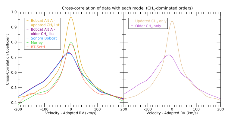
We have confirmed that the older CH₄ line lists are inaccurate in the 1.60–1.73 $\mu$m and 2.10–2.40 $\mu$m regions (see Section 4.2), and the inaccurate line positions could result in a non-detection of an exoplanet. We cross-correlated our data against the various models to showcase the improvement that the newer CH₄ lines offer in a cross-correlation analysis. We used the IDL function c_correlate and included only the CH₄-dominated orders of the $H$ and $K$ bands ($m=$ 112–104, 1.594–1.730 $\mu$m; $m=$ 85–77, 2.084–2.294 $\mu$m). The model parameters were fixed to the values given in Table 3. The results of the cross-correlations are shown in Fig. 14.

To isolate the effects of the choice of CH₄ line list our cross-correlation analysis includes two different Bobcat Alternative A models: one with the updated CH₄ line lists and one with the older CH₄ line lists used in the Sonora Bobcat models, while keeping the H₂O, CO, NH₃, and H₂S line lists the same as in the newest models (see Table 4). As seen in the left panel of Fig. 14, the peak of the Bobcat Alternative A model with the newest CH₄ line lists is the highest. The peak for the Bobcat Alternative A model with the older CH₄ line lists is significantly lower. In fact, the latter is nearly identical to the cross-correlation peak for the Sonora Bobcat model. This is as expected, as these two models use the same underlying atmospheric model, and we showed previously that the choice of line lists for the other molecules has less impact on the quality of the model fits to the data. We see that the peak of the Bobcat Alternative A model with the older CH₄ line lists is slightly higher than the peak of the Sonora Bobcat model, likely due to the newer line lists used for the other molecules, particularly H₂O. We also see that the CH₄ line lists used in the Sonora Bobcat models result in an offset in the peak towards negative velocities. This is consistent with the lower radial velocities we found for the Sonora Bobcat model in orders where CH₄ was the main absorber (Fig. 3 and 4).

The importance of the choice of CH₄ line lists in the methane-dominated IGRINS orders is demonstrated in the right panel of Fig. 14. That figure compares the cross-correlation functions of our data with versions of the models that include only methane absorption and ignore the contributions from H₂O, CO, NH₃, and H₂S. The ‘Updated CH₄ only’ models uses the line list incorporated in the Bobcat Alternative A models, while the ‘Older CH₄ only’ uses the line lists incorporated in the Sonora Bobcat models. The ‘updated’ and ‘older’ cross-correlations are very similar in shape and peak strengths to the Bobcat Alternative A model and Sonora Bobcat cross-correlations, respectively. This is not surprising, as we have performed the cross-correlation specifically for the CH₄-dominated orders, and so models which include additional molecules provide only a small improvement.

In their analysis of the $K$-band spectra of HD 209458 b and $\beta$ Pictoris b, Snellen et al. (2010, 2014) were successful in detecting CO through cross-correlation with atmospheric models, but failed to recover CH₄. Inaccurate line lists could be responsible for these non-detections, as these studies used the older HITRAN’08 (Rothman et al., 2009) for their CH₄ line lists. The atmosphere of $\beta$ Pictoris b may also be too hot for the detection of CH₄ ($T_{\rm eff}=1724$ K; Chilcote et al. 2017), but CH₄ may be detectable in HD 209458 b ($T_{\rm eq}=1449$ K; Torres et al. 2008) with an improved line list. Indeed, more recently, Guilluy et al. (2019) and Giacobbe et al. (2021) had success detecting CH₄ from HD 102195 b and HD 209458 b, respectively, with more up-to-date line lists. Guilluy et al. (2019) used HITRAN2012 (Rothman et al., 2013), and Giacobbe et al. (2021) used Hargreaves et al. (2020), the same CH₄ line list used in the Bobcat Alternative A models. A separate demonstration of the enhanced utility of the newer Hargreaves et al. (2020) CH₄ line lists is evident in Line et al. (2021), who determined the C/H, O/H, and C/O ratios of the hot Jupiter WASP-77Ab ($T_{\rm eff}=1740$ K; Maxted et al. 2013) using cross-correlation methods with IGRINS data.

Figure 14: Left panel: Cross-correlations of the data with each of the model families, including a version of the Bobcat Alternative A model modified to use the older CH₄ line list (the other molecules use the newer line lists given in Table 4). We performed this cross correlation across the CH₄-dominated orders of both the $H$ and $K$ bands for models with parameters given in Table 3. As expected, the peak of the Bobcat Alternative A model that uses the newest CH₄ line lists is higher than for the other models. Right panel: The same as the left panel, but for Bobcat Alternative A models that incorporate only CH₄. The ‘Updated CH₄-only’ model uses the line list used in the new Bobcat Alternative A model, while the ‘Older CH₄-only’ model uses the line list used in the Sonora Bobcat model.

7 Conclusions

The data presented here are among the highest resolution spectra ever published for a cold brown dwarf. We found that model spectra with the most recent line lists showed significant improvement in fitting the observed spectrum of the T6 dwarf 2MASS J08173001$-$6155158. The updated line lists for water, methane, and ammonia allow for precise empirical determinations of physical parameters. We identified the most reliable regions for measuring physical parameters of cold brown dwarfs, and we summarized our findings in Section 5. In particular, we highlighted the excellent fits of the Sonora Bobcat Alternative A models (Hood et al. in preparation), and the accuracy of the ExoMol/POKAZATEL line list for H₂O (Polyansky et al., 2018) and the HITEMP line list for CH₄ (Hargreaves et al., 2020) in matching the observed spectrum. We confirmed that like other late-type T and Y dwarfs, 2M0817 demonstrates CO disequilibrium chemistry. We identified individual NH₃ lines in the spectrum of 2M0817, and we presented the first unambiguous detections of H₂S and H₂ absorption in an extra-solar atmosphere. Our molecular hydrogen detection allowed us to place a semi-empirical upper limit on the atmospheric dust concentration of this brown dwarf. We found that the atmosphere of 2M0817 has $>$500 times less dust than the ISM, implying that the atmosphere is almost completely dust-free. Additionally, we identified several spectroscopic features that are missing from, or are poorly fit by the models. Finally, our cross-correlation analysis showed that the most up-to-date line lists are significantly more sensitive to CH₄ absorption in the atmosphere of this T6 dwarf. This will improve the detectability of CH₄ and other atmospheric absorbers in more challenging observations, such as the high-dispersion, low-SNR, high-background spectra of exoplanets around their host stars.

Data Availability

The raw IGRINS data for 2MASS J08173001$-$6155158 are available on the Gemini Archive under Program ID GS-2018A-Q-304. The reduced spectrum and best-fitting Bobcat Alternative A spectra are available through the Harvard Dataverse (https://doi.org/10.7910/DVN/DV1ZLR) or Zenodo (https://doi.org/10.5281/zenodo.6082001).

Appendix A The Full Suite of Model Fits for Every IGRINS Order

We show the best fitting Bobcat Alternative A models for all orders in the IGRINS spectrum in figures  15 ($H$ band) and 28 ($K$ band).

Figure 15: Every order of the $H$ band. The model shown is the best fitting Bobcat Alternative A model for each order. Each order is fit independently (Section 3), so the physical parameters may differ between orders. The top panel shows the molecule-by-molecule breakdown of the model. The second panel from the top shows the IGRINS data with the full model. The second panel from the bottom shows the residuals on the same $y$-scale as the panel above it. The model discrepancies listed in Table 5 are indicated in these figures with black arrows for discrepant lines, and black brackets for discrepant regions. The bottom panel shows the PSG Earth’s transmittance to help assess the telluric lines in our spectra. The OH emission lines are also shown as boxes and indicate position only, not line strength. Wider boxes indicate blended OH emission lines. A dashed horizontal line indicates the 65 per cent absorption threshold used for our telluric mask. The $\Delta\chi^{2}_{\rm reduced}$ is the difference between the displayed order’s $\chi^{2}_{\rm reduced}$, and the $\chi^{2}_{\rm reduced}$ of the best fitting order ($m=85$, Fig. 28). This figure continues for many pages, with two orders per page, to show all 26 orders of the $H$ band.

Figure 16: Continued.

Figure 17: Continued.

Figure 18: Continued.

Figure 19: Continued.

Figure 20: Continued.

Figure 21: Continued.

Figure 22: Continued.

Figure 23: Continued.

Figure 24: Continued.

Figure 25: Continued.

Figure 26: Continued.

Figure 27: Continued.

Figure 28: The same as Fig. 15, but for the $K$ band. This figure continues for many pages, with two orders per page, to show all 23 orders of the $K$ band.

Figure 29: Continued.

Figure 30: Continued.

Figure 31: Continued.

Figure 32: Continued.

Figure 33: Continued.

Figure 34: Continued.

Figure 35: Continued.

Figure 36: Continued.

Figure 37: Continued.

Figure 38: Continued.

Figure 39: Continued.

References

- Ackerman & Marley (2001) Ackerman A. S., Marley M. S., 2001, ApJ, 556, 872
- Allard & Hauschildt (1995) Allard F., Hauschildt P. H., 1995, ApJ, 445, 433
- Allard et al. (2012) Allard F., Homeier D., Freytag B., 2012, Philosophical Transactions of the Royal Society of London Series A, 370, 2765
- Allard et al. (2014) Allard F., Homeier D., Freytag B., 2014, in Astronomical Society of India Conference Series. pp 33–45
- Artigau et al. (2010) Artigau É., Radigan J., Folkes S., Jayawardhana R., Kurtev R., Lafrenière D., Doyon R., Borissova J., 2010, ApJ, 718, L38
- Azzam et al. (2015) Azzam A. A. A., Lodi L., Yurchenko S. N., Tennyson J., 2015, J. Quant. Spectrosc. Radiative Transfer, 161, 41
- Barber et al. (2006) Barber R. J., Tennyson J., Harris G. J., Tolchenov R. N., 2006, MNRAS, 368, 1087
- Beichman et al. (2014) Beichman C., Gelino C. R., Kirkpatrick J. D., Cushing M. C., Dodson-Robinson S., Marley M. S., Morley C. V., Wright E. L., 2014, ApJ, 783, 68
- Bochanski et al. (2011) Bochanski J. J., Burgasser A. J., Simcoe R. A., West A. A., 2011, AJ, 142, 169
- Burgasser et al. (2006) Burgasser A. J., Geballe T. R., Leggett S. K., Kirkpatrick J. D., Golimowski D. A., 2006, ApJ, 637, 1067
- Burrows & Sharp (1999) Burrows A., Sharp C. M., 1999, ApJ, 512, 843
- Burrows et al. (1997) Burrows A., et al., 1997, ApJ, 491, 856
- Burrows et al. (2001) Burrows A., Hubbard W. B., Lunine J. I., Liebert J., 2001, Reviews of Modern Physics, 73, 719
- Canty et al. (2015) Canty J. I., et al., 2015, MNRAS, 450, 454
- Cardelli et al. (1989) Cardelli J. A., Clayton G. C., Mathis J. S., 1989, ApJ, 345, 245
- Chilcote et al. (2017) Chilcote J., et al., 2017, AJ, 153, 182
- Coles et al. (2019) Coles P. A., Yurchenko S. N., Tennyson J., 2019, MNRAS, 490, 4638
- Cushing et al. (2006) Cushing M. C., et al., 2006, ApJ, 648, 614
- Cushing et al. (2011) Cushing M. C., et al., 2011, ApJ, 743, 50
- Cushing et al. (2021) Cushing M. C., et al., 2021, ApJ, 920, 20
- Fegley & Lodders (1994) Fegley Bruce J., Lodders K., 1994, Icarus, 110, 117
- Fegley & Lodders (1996) Fegley Bruce J., Lodders K., 1996, ApJ, 472, L37
- Filippazzo et al. (2015) Filippazzo J. C., Rice E. L., Faherty J., Cruz K. L., Van Gordon M. M., Looper D. L., 2015, ApJ, 810, 158
- Fortney et al. (2008) Fortney J. J., Marley M. S., Saumon D., Lodders K., 2008, ApJ, 683, 1104
- Freedman et al. (2014) Freedman R. S., Lustig-Yaeger J., Fortney J. J., Lupu R. E., Marley M. S., Lodders K., 2014, ApJS, 214, 25
- Gaia Collaboration (2016) Gaia Collaboration 2016, A&A, 595, A1
- Gaia Collaboration (2021) Gaia Collaboration 2021, A&A, 649, A1
- Gautier et al. (1976) Gautier T. N. I., Fink U., Treffers R. R., Larson H. P., 1976, ApJ, 207, L129
- Geballe et al. (1996) Geballe T. R., Kulkarni S. R., Woodward C. E., Sloan G. C., 1996, ApJ, 467, L101
- Geballe et al. (2009) Geballe T. R., Saumon D., Golimowski D. A., Leggett S. K., Marley M. S., Noll K. S., 2009, ApJ, 695, 844
- Giacobbe et al. (2021) Giacobbe P., et al., 2021, Nature, 592, 205
- Golimowski et al. (2004) Golimowski D. A., et al., 2004, AJ, 127, 3516
- Goorvitch (1994) Goorvitch D., 1994, ApJS, 95, 535
- Gordon et al. (2017) Gordon I. E., et al., 2017, J. Quant. Spectrosc. Radiative Transfer, 203, 3
- Gordon et al. (2022) Gordon I. E., et al., 2022, J. Quant. Spectrosc. Radiative Transfer, 277, 107949
- Gorenstein (1975) Gorenstein P., 1975, ApJ, 198, 95
- Gray (1992) Gray D. F., 1992, The observation and analysis of stellar photospheres.. Cambridge University Press
- Guilluy et al. (2019) Guilluy G., Sozzetti A., Brogi M., Bonomo A. S., Giacobbe P., Claudi R., Benatti S., 2019, A&A, 625, A107
- Habart et al. (2005) Habart E., Walmsley M., Verstraete L., Cazaux S., Maiolino R., Cox P., Boulanger F., Pineau des Forêts G., 2005, Space Sci. Rev., 119, 71
- Hargreaves et al. (2020) Hargreaves R. J., Gordon I. E., Rey M., Nikitin A. V., Tyuterev V. G., Kochanov R. V., Rothman L. S., 2020, ApJS, 247, 55
- Hauschildt et al. (1999) Hauschildt P. H., Allard F., Baron E., 1999, ApJ, 512, 377
- Helling et al. (2019) Helling C., Gourbin P., Woitke P., Parmentier V., 2019, A&A, 626, A133
- Irwin et al. (2018) Irwin P. G. J., Toledo D., Garland R., Teanby N. A., Fletcher L. N., Orton G. A., Bézard B., 2018, Nature Astronomy, 2, 420
- Irwin et al. (2019) Irwin P. G. J., Toledo D., Garland R., Teanby N. A., Fletcher L. N., Orton G. S., Bézard B., 2019, Icarus, 321, 550
- Kim et al. (1995) Kim S. J., Trafton L. M., Geballe T. R., Slanina Z., 1995, Icarus, 113, 217
- Lee et al. (2017) Lee J.-J., Gullikson K., Kaplan K., 2017, igrins/plp 2.2.0, doi:10.5281/zenodo.845059, https://doi.org/10.5281/zenodo.845059
- Léger et al. (1996) Léger A., Mariotti J. M., Mennesson B., Ollivier M., Puget J. L., Rouan D., Schneider J., 1996, Icarus, 123, 249
- Leggett et al. (2012) Leggett S. K., et al., 2012, ApJ, 748, 74
- Leggett et al. (2019) Leggett S. K., et al., 2019, ApJ, 882, 117
- Li et al. (2015) Li G., Gordon I. E., Rothman L. S., Tan Y., Hu S.-M., Kassi S., Campargue A., Medvedev E. S., 2015, ApJS, 216, 15
- Line et al. (2015) Line M. R., Teske J., Burningham B., Fortney J. J., Marley M. S., 2015, ApJ, 807, 183
- Line et al. (2017) Line M. R., et al., 2017, ApJ, 848, 83
- Line et al. (2021) Line M. R., et al., 2021, Nature, 598, 580
- Lodders & Fegley (2002) Lodders K., Fegley B., 2002, Icarus, 155, 393
- Lodders & Fegley (2006) Lodders K., Fegley B. J., 2006, Chemistry of Low Mass Substellar Objects. p. 1, doi:10.1007/3-540-30313-8_1
- Luhman & Esplin (2016) Luhman K. L., Esplin T. L., 2016, AJ, 152, 78
- Lupu et al. (2014) Lupu R. E., et al., 2014, ApJ, 784, 27
- Mace et al. (2016) Mace G., et al., 2016, in Evans C. J., Simard L., Takami H., eds, Society of Photo-Optical Instrumentation Engineers (SPIE) Conference Series Vol. 9908, Ground-based and Airborne Instrumentation for Astronomy VI. p. 99080C, doi:10.1117/12.2232780
- Mace et al. (2018) Mace G., et al., 2018, in Evans C. J., Simard L., Takami H., eds, Society of Photo-Optical Instrumentation Engineers (SPIE) Conference Series Vol. 10702, Ground-based and Airborne Instrumentation for Astronomy VII. p. 107020Q, doi:10.1117/12.2312345
- Marley & Robinson (2015) Marley M. S., Robinson T. D., 2015, ARA&A, 53, 279
- Marley et al. (1996) Marley M. S., Saumon D., Guillot T., Freedman R. S., Hubbard W. B., Burrows A., Lunine J. I., 1996, Science, 272, 1919
- Marley et al. (2021) Marley M. S., et al., 2021, ApJ, 920, 85
- Maxted et al. (2013) Maxted P. F. L., et al., 2013, PASP, 125, 48
- Miles et al. (2020) Miles B. E., et al., 2020, AJ, 160, 63
- Morley et al. (2012) Morley C. V., Fortney J. J., Marley M. S., Visscher C., Saumon D., Leggett S. K., 2012, ApJ, 756, 172
- Morley et al. (2015) Morley C. V., Fortney J. J., Marley M. S., Zahnle K., Line M., Kempton E., Lewis N., Cahoy K., 2015, ApJ, 815, 110
- Niemann et al. (1998) Niemann H. B., et al., 1998, J. Geophys. Res., 103, 22831
- Noll et al. (1988) Noll K. S., Knacke R. F., Geballe T. R., Tokunaga A. T., 1988, ApJ, 324, 1210
- Noll et al. (1995) Noll K. S., et al., 1995, Science, 267, 1307
- Noll et al. (1997) Noll K. S., Geballe T. R., Marley M. S., 1997, ApJ, 489, L87
- Noll et al. (2000) Noll K. S., Geballe T. R., Leggett S. K., Marley M. S., 2000, ApJ, 541, L75
- Oppenheimer et al. (1995) Oppenheimer B. R., Kulkarni S. R., Matthews K., Nakajima T., 1995, Science, 270, 1478
- Oppenheimer et al. (1998) Oppenheimer B. R., Kulkarni S. R., Matthews K., van Kerkwijk M. H., 1998, ApJ, 502, 932
- Park et al. (2014) Park C., et al., 2014, in Ramsay S. K., McLean I. S., Takami H., eds, Society of Photo-Optical Instrumentation Engineers (SPIE) Conference Series Vol. 9147, Ground-based and Airborne Instrumentation for Astronomy V. p. 91471D, doi:10.1117/12.2056431
- Partridge & Schwenke (1997) Partridge H., Schwenke D. W., 1997, J. Chem. Phys., 106, 4618
- Polyansky et al. (2018) Polyansky O. L., Kyuberis A. A., Zobov N. F., Tennyson J., Yurchenko S. N., Lodi L., 2018, MNRAS, 480, 2597
- Prinn & Barshay (1977) Prinn R. G., Barshay S. S., 1977, Science, 198, 1031
- Radigan et al. (2014) Radigan J., Lafrenière D., Jayawardhana R., Artigau E., 2014, ApJ, 793, 75
- Roellig et al. (2004) Roellig T. L., et al., 2004, ApJS, 154, 418
- Rothman et al. (2005) Rothman L. S., et al., 2005, J. Quant. Spectrosc. Radiative Transfer, 96, 139
- Rothman et al. (2009) Rothman L. S., et al., 2009, J. Quant. Spectrosc. Radiative Transfer, 110, 533
- Rothman et al. (2010) Rothman L. S., et al., 2010, J. Quant. Spectrosc. Radiative Transfer, 111, 2139
- Rothman et al. (2013) Rothman L. S., et al., 2013, J. Quant. Spectrosc. Radiative Transfer, 130, 4
- Roueff et al. (2019) Roueff E., Abgrall H., Czachorowski P., Pachucki K., Puchalski M., Komasa J., 2019, A&A, 630, A58
- Rousselot et al. (2000) Rousselot P., Lidman C., Cuby J. G., Moreels G., Monnet G., 2000, A&A, 354, 1134
- Saumon et al. (2000) Saumon D., Geballe T. R., Leggett S. K., Marley M. S., Freedman R. S., Lodders K., Fegley B. J., Sengupta S. K., 2000, ApJ, 541, 374
- Saumon et al. (2003) Saumon D., Marley M. S., Lodders K., Freedman R. S., 2003, in Martín E., ed., Proceedings of IAU Vol. 211, Brown Dwarfs. p. 345 (arXiv:astro-ph/0207070)
- Saumon et al. (2012) Saumon D., Marley M. S., Abel M., Frommhold L., Freedman R. S., 2012, ApJ, 750, 74
- Schneider et al. (2015) Schneider A. C., et al., 2015, ApJ, 804, 92
- Scoville et al. (1983) Scoville N., Kleinmann S. G., Hall D. N. B., Ridgway S. T., 1983, ApJ, 275, 201
- Seager et al. (2013) Seager S., Bains W., Hu R., 2013, ApJ, 775, 104
- Sharp & Burrows (2007) Sharp C. M., Burrows A., 2007, ApJS, 168, 140
- Showman et al. (2020) Showman A. P., Tan X., Parmentier V., 2020, Space Sci. Rev., 216, 139
- Skrutskie et al. (2006) Skrutskie M. F., et al., 2006, AJ, 131, 1163
- Snellen et al. (2010) Snellen I. A. G., de Kok R. J., de Mooij E. J. W., Albrecht S., 2010, Nature, 465, 1049
- Snellen et al. (2014) Snellen I. A. G., Brandl B. R., de Kok R. J., Brogi M., Birkby J., Schwarz H., 2014, Nature, 509, 63
- Sorahana & Yamamura (2012) Sorahana S., Yamamura I., 2012, ApJ, 760, 151
- Sousa-Silva et al. (2015) Sousa-Silva C., Al-Refaie A. F., Tennyson J., Yurchenko S. N., 2015, MNRAS, 446, 2337
- Stahl et al. (2021) Stahl A. G., et al., 2021, AJ, 161, 283
- Strong et al. (1993) Strong K., Taylor F. W., Calcutt S. B., Remedios J. J., Ballard J., 1993, J. Quant. Spectrosc. Radiative Transfer, 50, 363
- Suárez et al. (2021) Suárez G., Metchev S., Leggett S. K., Saumon D., Marley M. S., 2021, ApJ, 920, 99
- Tannock et al. (2021) Tannock M. E., et al., 2021, AJ, 161, 224
- Tennyson & Yurchenko (2012) Tennyson J., Yurchenko S. N., 2012, MNRAS, 425, 21
- Tennyson & Yurchenko (2018) Tennyson J., Yurchenko S., 2018, Atoms, 6, 26
- Torres et al. (2008) Torres G., Winn J. N., Holman M. J., 2008, ApJ, 677, 1324
- Trafton et al. (1997) Trafton L. M., Kim S. J., Geballe T. R., Miller S., 1997, Icarus, 130, 544
- Villanueva et al. (2018) Villanueva G. L., Smith M. D., Protopapa S., Faggi S., Mandell A. M., 2018, J. Quant. Spectrosc. Radiative Transfer, 217, 86
- Wenger & Champion (1998) Wenger C., Champion J. P., 1998, J. Quant. Spectrosc. Radiative Transfer, 59, 471
- Yuk et al. (2010) Yuk I.-S., et al., 2010, in McLean I. S., Ramsay S. K., Takami H., eds, Society of Photo-Optical Instrumentation Engineers (SPIE) Conference Series Vol. 7735, Ground-based and Airborne Instrumentation for Astronomy III. p. 77351M, doi:10.1117/12.856864
- Yurchenko & Tennyson (2014) Yurchenko S. N., Tennyson J., 2014, MNRAS, 440, 1649
- Yurchenko et al. (2011) Yurchenko S. N., Barber R. J., Tennyson J., 2011, MNRAS, 413, 1828
- Yurchenko et al. (2013) Yurchenko S. N., Tennyson J., Barber R. J., Thiel W., 2013, Journal of Molecular Spectroscopy, 291, 69
- Zalesky et al. (2019) Zalesky J. A., Line M. R., Schneider A. C., Patience J., 2019, ApJ, 877, 24