Computational Doob’s hh-transforms for Online Filtering of Discretely Observed Diffusions

Nicolas Chopin    Andras Fulop    Jeremy Heng    Alexandre H. Thiery
Abstract

This paper is concerned with online filtering of discretely observed nonlinear diffusion processes. Our approach is based on the fully adapted auxiliary particle filter, which involves Doob’s hh-transforms that are typically intractable. We propose a computational framework to approximate these hh-transforms by solving the underlying backward Kolmogorov equations using nonlinear Feynman-Kac formulas and neural networks. The methodology allows one to train a locally optimal particle filter prior to the data-assimilation procedure. Numerical experiments illustrate that the proposed approach can be orders of magnitude more efficient than state-of-the-art particle filters in the regime of highly informative observations, when the observations are extreme under the model, or if the state dimension is large.

Particle filtering, Diffusions, Doob’s transform

1 Introduction

Diffusion processes are fundamental tools in applied mathematics, statistics, and machine learning. Because this flexible class of models is easily amenable to computations and simulations, diffusion processes are very common in biological sciences (e.g. population and multi-species models, stochastic delay population systems), neuroscience (e.g. models for synaptic input, stochastic Hodgkin–Huxley model, stochastic Fitzhugh–Nagumo model), and finance (e.g. modeling multi assets prices) (Allen, 2010; Shreve et al., 2004; Capasso & Capasso, 2021). In these disciplines, tracking signals from partial or noisy observations is a very common task. However, working with diffusion processes can be challenging as their transition densities are only tractable in rare and simple situations such as (geometric) Brownian motions or Ornstein–Uhlenbeck (OU) processes. This difficulty has hindered the use of standard methodologies for inference and data-assimilation of models driven by diffusion processes and various approaches have been developed to circumvent or mitigate some of these issues, as discussed in Section 4.

Consider a time-homogeneous multivariate diffusion process d𝐗t=μ(𝐗t)dt+σ(𝐗t)d𝐁t𝑑subscript𝐗𝑡𝜇subscript𝐗𝑡𝑑𝑡𝜎subscript𝐗𝑡𝑑subscript𝐁𝑡d\mathbf{X}_{t}=\mu(\mathbf{X}_{t})\,dt+\sigma(\mathbf{X}_{t})\,d\mathbf{B}_{t} that is discretely observed at regular intervals. Noisy observations 𝐲ksubscript𝐲𝑘\mathbf{y}_{k} of the latent process 𝐗tksubscript𝐗subscript𝑡𝑘\mathbf{X}_{t_{k}} are collected at equispaced times tkkTsubscript𝑡𝑘𝑘𝑇t_{k}\equiv k\,T for k1𝑘1k\geq 1. We consider the online filtering problem which consists in estimating the conditional laws πk(d𝐱)=(𝐗tkd𝐱|𝐲1,,𝐲k)subscript𝜋𝑘𝑑𝐱subscript𝐗subscript𝑡𝑘conditional𝑑𝐱subscript𝐲1subscript𝐲𝑘\pi_{k}(d\mathbf{x})=\mathbb{P}(\mathbf{X}_{t_{k}}\in d\mathbf{x}|\mathbf{y}_{1},\ldots,\mathbf{y}_{k}), i.e. the filtering distributions, as observations are collected. We focus on the use of Particle Filters (PFs) that approximate the filtering distributions with a system of weighted particles. Although many previous works have relied on the Bootstrap Particle Filter (BPF), which simulates particles from the diffusion process, it can perform poorly in challenging scenarios as it fails to take the incoming observation 𝐲ksubscript𝐲𝑘\mathbf{y}_{k} into account. This issue is partially mitigated in Guided Intermediate Resampling Filters (GIRF) by relying on resampling at intermediate times between observations using guiding functions that forecast the likelihood of future observations (Del Moral & Murray, 2015; Park & Ionides, 2020).

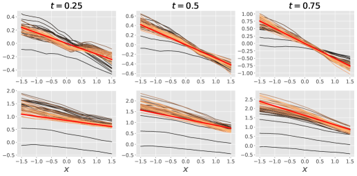
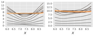
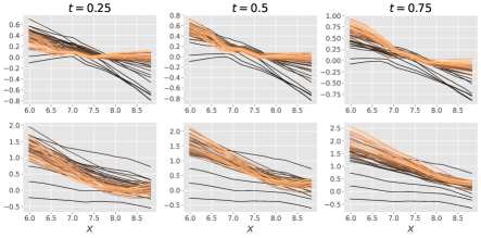
The (locally) optimal approach given by the Fully Adapted Auxiliary Particle Filter (FA-APF) (Pitt & Shephard, 1999; Doucet et al., 2000) can only be implemented in simple settings such as finite state-spaces or linear and Gaussian models. We show in this article that the FA-APF can be practically implemented in a much larger class of models; see Figure 1(a) for a comparison between the FA-APF and the BPF. The proposed method simulates a conditioned diffusion process, which can be formulated as a control problem involving an intractable Doob’s hh-transform (Rogers & Williams, 2000; Chung & Walsh, 2006); see Figure 1(b) for an illustration. We propose the Computational Doob’s hh-Transform (CDT) framework for efficiently approximating these quantities. Since the latent process is a diffusion process, the Doob’s hh-transform satisfies the backward Kolmogorov equation: our proposed method relies on nonlinear Feynman-Kac formulas for solving this backward Kolmogorov partial differential equation simultaneously for all possible observations. Importantly, this preprocessing step only needs to be performed once before starting the online filtering procedure. Numerical experiments illustrate that the proposed approach can be orders of magnitude more efficient than the BPF in the regime of highly informative observations, when the observations are extreme under the model, or if the state dimension is large. A PyTorch implementation to reproduce our numerical experiments is available at https://anonymous.4open.science/r/CompDoobTransform/.

Notations.

For two matrices A,Bd,d𝐴𝐵superscript𝑑𝑑A,B\in\mathbb{R}^{d,d}, their Frobenius inner product is defined as A,BF=i,j=1dAi,jBi,jsubscript𝐴𝐵Fsuperscriptsubscript𝑖𝑗1𝑑subscript𝐴𝑖𝑗subscript𝐵𝑖𝑗\langle A,B\rangle_{\mathrm{F}}=\sum_{i,j=1}^{d}A_{i,j}B_{i,j}. The Euclidean inner product for 𝐮,𝐯d𝐮𝐯superscript𝑑\mathbf{u},\mathbf{v}\in\mathbb{R}^{d} is denoted as 𝐮,𝐯=i=1duivi𝐮𝐯superscriptsubscript𝑖1𝑑subscript𝑢𝑖subscript𝑣𝑖\langle\mathbf{u},\mathbf{v}\rangle=\sum_{i=1}^{d}u_{i}v_{i}. For two (or more) functions F𝐹F and G𝐺G, we sometimes use the notation [FG](𝐱)F(𝐱)G(𝐱)delimited-[]𝐹𝐺𝐱𝐹𝐱𝐺𝐱[FG](\mathbf{x})\equiv F(\mathbf{x})G(\mathbf{x}). For a function φ:d:𝜑superscript𝑑\varphi:\mathbb{R}^{d}\to\mathbb{R}, the gradient and its Hessian matrix are denoted as φ(𝐱)d𝜑𝐱superscript𝑑\nabla\varphi(\mathbf{x})\in\mathbb{R}^{d} and 2φ(𝐱)d,dsuperscript2𝜑𝐱superscript𝑑𝑑\nabla^{2}\varphi(\mathbf{x})\in\mathbb{R}^{d,d}. The Dirac measure centred at x0subscript𝑥0x_{0} is denoted as δ(d𝐱;𝐱0)𝛿𝑑𝐱subscript𝐱0\delta(d\mathbf{x};\mathbf{x}_{0}).

2 Background

2.1 Filtering of discretely observed diffusions

Consider a homogeneous diffusion process {𝐗t}t0subscriptsubscript𝐗𝑡𝑡0\{\mathbf{X}_{t}\}_{t\geq 0} in 𝒳=d𝒳superscript𝑑\mathcal{X}=\mathbb{R}^{d} with initial distribution ρ0(d𝐱)subscript𝜌0𝑑𝐱\rho_{0}(d\mathbf{x}) and dynamics

d𝐗t=μ(𝐗t)dt+σ(𝐗t)d𝐁t,𝑑subscript𝐗𝑡𝜇subscript𝐗𝑡𝑑𝑡𝜎subscript𝐗𝑡𝑑subscript𝐁𝑡\displaystyle d\mathbf{X}_{t}=\mu(\mathbf{X}_{t})\,dt+\sigma(\mathbf{X}_{t})\,d\mathbf{B}_{t}, (1)

described by the drift and volatility functions μ:dd:𝜇superscript𝑑superscript𝑑\mu:\mathbb{R}^{d}\to\mathbb{R}^{d} and σ:dd,d:𝜎superscript𝑑superscript𝑑𝑑\sigma:\mathbb{R}^{d}\to\mathbb{R}^{d,d}. The associated semi-group of transition probabilities ps(d𝐱^𝐱)subscript𝑝𝑠conditional𝑑^𝐱𝐱p_{s}(d\widehat{\mathbf{x}}\mid\mathbf{x}) satisfies (𝐗t+sA𝐗t=𝐱)=Aps(d𝐱^𝐱)subscript𝐗𝑡𝑠conditional𝐴subscript𝐗𝑡𝐱subscript𝐴subscript𝑝𝑠conditional𝑑^𝐱𝐱\mathbb{P}(\mathbf{X}_{t+s}\in A\mid\mathbf{X}_{t}=\mathbf{x})=\int_{A}p_{s}(d\widehat{\mathbf{x}}\mid\mathbf{x}) for any s,t>0𝑠𝑡0s,t>0 and measurable A𝒳𝐴𝒳A\subset\mathcal{X}. The process {𝐁t}t0subscriptsubscript𝐁𝑡𝑡0\{\mathbf{B}_{t}\}_{t\geq 0} is a standard dsuperscript𝑑\mathbb{R}^{d}-valued Brownian motion. The diffusion process {𝐗t}t0subscriptsubscript𝐗𝑡𝑡0\{\mathbf{X}_{t}\}_{t\geq 0} is discretely observed at time tk=kTsubscript𝑡𝑘𝑘𝑇t_{k}=kT, for k1𝑘1k\geq 1, for some inter-observation time T>0𝑇0T>0. The 𝒴𝒴\mathcal{Y}-valued observation 𝐘k𝒴subscript𝐘𝑘𝒴\mathbf{Y}_{k}\in\mathcal{Y} at time tksubscript𝑡𝑘t_{k} is modelled by the likelihood function g:𝒳×𝒴+:𝑔𝒳𝒴subscriptg:\mathcal{X}\times\mathcal{Y}\to\mathbb{R}_{+}, i.e. for any measurable A𝒴𝐴𝒴A\subset\mathcal{Y}, we have (𝐘kA𝐗tk=𝐱k)=Ag(𝐱k,𝐲)𝑑𝐲subscript𝐘𝑘conditional𝐴subscript𝐗subscript𝑡𝑘subscript𝐱𝑘subscript𝐴𝑔subscript𝐱𝑘𝐲differential-d𝐲\mathbb{P}(\mathbf{Y}_{k}\in A\mid\mathbf{X}_{t_{k}}=\mathbf{x}_{k})=\int_{A}g(\mathbf{x}_{k},\mathbf{y})\,d\mathbf{y} for some dominating measure d𝐲𝑑𝐲d\mathbf{y} on 𝒴𝒴\mathcal{Y}. The operator \mathcal{L} denotes the generator of the diffusion process {𝐗t}t0subscriptsubscript𝐗𝑡𝑡0\{\mathbf{X}_{t}\}_{t\geq 0}, defined by φ=μ,φ+12σσ,2φF𝜑𝜇𝜑12subscript𝜎superscript𝜎topsuperscript2𝜑F\mathcal{L}\varphi=\langle\mu,\nabla\varphi\rangle+\frac{1}{2}\,\langle\sigma\sigma^{\top},\nabla^{2}\varphi\rangle_{\mathrm{F}} for test function φ:𝒳:𝜑𝒳\varphi:\mathcal{X}\to\mathbb{R}. This article is concerned with approximating the filtering distributions πk(d𝐱)=(𝐗tkd𝐱𝐲1,,𝐲k).subscript𝜋𝑘𝑑𝐱subscript𝐗subscript𝑡𝑘conditional𝑑𝐱subscript𝐲1subscript𝐲𝑘\pi_{k}(d\mathbf{x})=\mathbb{P}(\mathbf{X}_{t_{k}}\in d\mathbf{x}\mid\mathbf{y}_{1},\ldots,\mathbf{y}_{k}). For convenience, we set π0(d𝐱)ρ0(d𝐱)subscript𝜋0𝑑𝐱subscript𝜌0𝑑𝐱\pi_{0}(d\mathbf{x})\equiv\rho_{0}(d\mathbf{x}) since there is no observation collected at the initial time t=0𝑡0t=0.

2.2 Particle filtering

Particle Filters (PF), also known as Sequential Monte Carlo (SMC) methods, are a set of Monte Carlo (MC) algorithms that can be used to solve filtering problems (see Chopin et al. (2020) for a recent textbook on the topic). PFs evolve a set of M1𝑀1M\geq 1 particles 𝐱t1:M=(𝐱t1,,𝐱tM)𝒳Msubscriptsuperscript𝐱:1𝑀𝑡subscriptsuperscript𝐱1𝑡subscriptsuperscript𝐱𝑀𝑡superscript𝒳𝑀\mathbf{x}^{1:M}_{t}=(\mathbf{x}^{1}_{t},\ldots,\mathbf{x}^{M}_{t})\in\mathcal{X}^{M} forward in time using a combination of propagation and resampling operations. To initialize the PF, each initial particle 𝐱0j𝒳subscriptsuperscript𝐱𝑗0𝒳\mathbf{x}^{j}_{0}\in\mathcal{X} for 1jM1𝑗𝑀1\leq j\leq M is sampled independently from the distribution ρ0(d𝐱)subscript𝜌0𝑑𝐱\rho_{0}(d\mathbf{x}) so that π0(d𝐱)M1j=1Mδ(d𝐱;𝐱0j)subscript𝜋0𝑑𝐱superscript𝑀1superscriptsubscript𝑗1𝑀𝛿𝑑𝐱subscriptsuperscript𝐱𝑗0\pi_{0}(d\mathbf{x})\approx M^{-1}\sum_{j=1}^{M}\delta(d\mathbf{x};\mathbf{x}^{j}_{0}). Approximations of the filtering distribution πksubscript𝜋𝑘\pi_{k} for k1𝑘1k\geq 1 are built recursively as follows. Given the MC approximation of the filtering distribution at time tksubscript𝑡𝑘t_{k}, πk(d𝐱)M1j=1Mδ(d𝐱;𝐱tkj)subscript𝜋𝑘𝑑𝐱superscript𝑀1superscriptsubscript𝑗1𝑀𝛿𝑑𝐱subscriptsuperscript𝐱𝑗subscript𝑡𝑘\pi_{k}(d\mathbf{x})\approx M^{-1}\sum_{j=1}^{M}\delta(d\mathbf{x};\mathbf{x}^{j}_{t_{k}}), the particles 𝐱tk1:Msubscriptsuperscript𝐱:1𝑀subscript𝑡𝑘\mathbf{x}^{1:M}_{t_{k}} are propagated independently forward in time by 𝐱^tk+1jqk+1(d𝐱^𝐱tkj)similar-tosubscriptsuperscript^𝐱𝑗subscript𝑡𝑘1subscript𝑞𝑘1conditional𝑑^𝐱subscriptsuperscript𝐱𝑗subscript𝑡𝑘\widehat{\mathbf{x}}^{j}_{t_{k+1}}\sim q_{k+1}(d\widehat{\mathbf{x}}\mid\mathbf{x}^{j}_{t_{k}}), using a Markov kernel qk+1(d𝐱^𝐱)subscript𝑞𝑘1conditional𝑑^𝐱𝐱q_{k+1}(d\widehat{\mathbf{x}}\mid\mathbf{x}) specified by the user. The BPF corresponds to the Markov kernel qk+1BPF(d𝐱^𝐱)=(𝐗tk+1d𝐱^𝐗tk=𝐱)superscriptsubscript𝑞𝑘1BPFconditional𝑑^𝐱𝐱subscript𝐗subscript𝑡𝑘1conditional𝑑^𝐱subscript𝐗subscript𝑡𝑘𝐱q_{k+1}^{\text{BPF}}(d\widehat{\mathbf{x}}\mid\mathbf{x})=\mathbb{P}(\mathbf{X}_{t_{k+1}}\in d\widehat{\mathbf{x}}\mid\mathbf{X}_{t_{k}}=\mathbf{x}), while the FA-APF (Pitt & Shephard, 1999) corresponds to the (typically intractable) kernel qk+1FA-APF(d𝐱^𝐱)=(𝐗tk+1d𝐱^𝐗tk=𝐱,𝐘k+1=𝐲k+1).q^{\text{FA-APF}}_{k+1}(d\widehat{\mathbf{x}}\mid\mathbf{x})=\mathbb{P}(\mathbf{X}_{t_{k+1}}\in d\widehat{\mathbf{x}}\mid\mathbf{X}_{t_{k}}=\mathbf{x},\mathbf{Y}_{{k+1}}=\mathbf{y}_{k+1}). Each particle 𝐱^tk+1jsubscriptsuperscript^𝐱𝑗subscript𝑡𝑘1\widehat{\mathbf{x}}^{j}_{t_{k+1}} is associated with a normalized weight W¯k+1j=Wk+1j/i=1MWk+1isubscriptsuperscript¯𝑊𝑗𝑘1subscriptsuperscript𝑊𝑗𝑘1superscriptsubscript𝑖1𝑀subscriptsuperscript𝑊𝑖𝑘1\overline{W}^{j}_{{k+1}}=W^{j}_{{k+1}}/\sum_{i=1}^{M}W^{i}_{{k+1}}, where the unnormalized weights Wk+1jsubscriptsuperscript𝑊𝑗𝑘1W^{j}_{{k+1}} (by time-homogeneity of (1)) are defined as

Wk+1j=pT(d𝐱^tk+1j𝐱tkj)qk+1(d𝐱^tk+1j𝐱tkj)g(𝐱^tk+1j,𝐲k+1).subscriptsuperscript𝑊𝑗𝑘1subscript𝑝𝑇conditional𝑑subscriptsuperscript^𝐱𝑗subscript𝑡𝑘1subscriptsuperscript𝐱𝑗subscript𝑡𝑘subscript𝑞𝑘1conditional𝑑subscriptsuperscript^𝐱𝑗subscript𝑡𝑘1subscriptsuperscript𝐱𝑗subscript𝑡𝑘𝑔subscriptsuperscript^𝐱𝑗subscript𝑡𝑘1subscript𝐲𝑘1\displaystyle W^{j}_{{k+1}}=\frac{p_{T}(d\widehat{\mathbf{x}}^{j}_{t_{k+1}}\mid\mathbf{x}^{j}_{t_{k}})}{q_{k+1}(d\widehat{\mathbf{x}}^{j}_{t_{k+1}}\mid\mathbf{x}^{j}_{t_{k}})}\,g(\widehat{\mathbf{x}}^{j}_{t_{k+1}},\mathbf{y}_{k+1}). (2)

The BPF and FA-APF correspond respectively to having

Wk+1j,BPF=g(𝐱^tk+1j,𝐲k+1),subscriptsuperscript𝑊𝑗BPF𝑘1𝑔subscriptsuperscript^𝐱𝑗subscript𝑡𝑘1subscript𝐲𝑘1\displaystyle W^{j,\text{BPF}}_{{k+1}}=g(\widehat{\mathbf{x}}^{j}_{t_{k+1}},\mathbf{y}_{k+1}), (3)
Wk+1j,FA-APF=𝔼[g(𝐗tk+1,𝐲k+1)𝐗tk=𝐱tkj].subscriptsuperscript𝑊𝑗FA-APF𝑘1𝔼delimited-[]conditional𝑔subscript𝐗subscript𝑡𝑘1subscript𝐲𝑘1subscript𝐗subscript𝑡𝑘subscriptsuperscript𝐱𝑗subscript𝑡𝑘\displaystyle W^{j,\text{FA-APF}}_{{k+1}}=\mathbb{E}[g(\mathbf{X}_{t_{k+1}},\mathbf{y}_{k+1})\mid\mathbf{X}_{t_{k}}=\mathbf{x}^{j}_{t_{k}}].

The weights are such that πk+1(d𝐱)j=1MW¯k+1jδ(d𝐱;𝐱tk+1j)subscript𝜋𝑘1𝑑𝐱superscriptsubscript𝑗1𝑀subscriptsuperscript¯𝑊𝑗𝑘1𝛿𝑑𝐱subscriptsuperscript𝐱𝑗subscript𝑡𝑘1\pi_{{k+1}}(d\mathbf{x})\approx\sum_{j=1}^{M}\overline{W}^{j}_{{k+1}}\,\delta(d\mathbf{x};\mathbf{x}^{j}_{t_{k+1}}). The resampling step consists in defining a new set of particles 𝐱tk+11:Msubscriptsuperscript𝐱:1𝑀subscript𝑡𝑘1\mathbf{x}^{1:M}_{t_{k+1}} with (𝐱tk+1j=𝐱^tk+1i)=W¯k+1isubscriptsuperscript𝐱𝑗subscript𝑡𝑘1subscriptsuperscript^𝐱𝑖subscript𝑡𝑘1subscriptsuperscript¯𝑊𝑖𝑘1\mathbb{P}(\mathbf{x}^{j}_{t_{k+1}}=\widehat{\mathbf{x}}^{i}_{t_{k+1}})=\overline{W}^{i}_{{k+1}}. This resampling scheme ensures that the equally weighted set of particles 𝐱tk+11:Msubscriptsuperscript𝐱:1𝑀subscript𝑡𝑘1\mathbf{x}^{1:M}_{t_{k+1}} provides a MC approximation of the filtering distribution at time tk+1subscript𝑡𝑘1t_{k+1} in the sense that πk+1(d𝐱)M1j=1Mδ(d𝐱;𝐱tk+1j)subscript𝜋𝑘1𝑑𝐱superscript𝑀1superscriptsubscript𝑗1𝑀𝛿𝑑𝐱subscriptsuperscript𝐱𝑗subscript𝑡𝑘1\pi_{{k+1}}(d\mathbf{x})\approx M^{-1}\sum_{j=1}^{M}\delta(d\mathbf{x};\mathbf{x}^{j}_{t_{k+1}}). Note that the particles 𝐱tk+11:Msubscriptsuperscript𝐱:1𝑀subscript𝑡𝑘1\mathbf{x}^{1:M}_{t_{k+1}} do not need to be resampled independently given the set of propagated particles 𝐱^tk+11:Msubscriptsuperscript^𝐱:1𝑀subscript𝑡𝑘1\widehat{\mathbf{x}}^{1:M}_{t_{k+1}}. We refer the reader to Gerber et al. (2019) for a recent discussion of resampling schemes within PFs and to Del Moral (2004) for a book-length treatment of the convergence properties of this class of MC methods. PF also returns an unbiased estimator ^(𝐲1,,𝐲K)=k=1K{M1j=1MWkj}^subscript𝐲1subscript𝐲𝐾superscriptsubscriptproduct𝑘1𝐾superscript𝑀1superscriptsubscript𝑗1𝑀subscriptsuperscript𝑊𝑗𝑘\widehat{\mathbb{P}}(\mathbf{y}_{1},\ldots,\mathbf{y}_{K})=\prod_{k=1}^{K}\{M^{-1}\sum_{j=1}^{M}W^{j}_{{k}}\} of the marginal likelihood of K1𝐾1K\geq 1 observations (𝐲1,,𝐲K)subscript𝐲1subscript𝐲𝐾\mathbb{P}(\mathbf{y}_{1},\ldots,\mathbf{y}_{K}). Hence by Jensen’s inequality, 𝔼[log^(𝐲1,,𝐲K)]𝔼delimited-[]^subscript𝐲1subscript𝐲𝐾\mathbb{E}[\log\widehat{\mathbb{P}}(\mathbf{y}_{1},\ldots,\mathbf{y}_{K})] is an evidence lower bound.

In most settings, the FA-APF (Pitt & Shephard, 1999) that minimizes a local variance criterion (Doucet et al., 2000) generates particles that are more consistent with informative data and weights that exhibit significantly less variability compared to the BPF and GIRF. This gain in efficiency can be very substantial when the signal-to-noise ratio is high or when observations contain outliers under the model specification. Nevertheless, implementing FA-APF requires sampling from the transition probability qk+1FA-APF(d𝐱^𝐱})q^{\text{FA-APF}}_{k+1}(d\widehat{\mathbf{x}}\mid\mathbf{x}\}), which is typically not feasible in practice. We will show in the following that this can be achieved in our setting by simulating a conditioned diffusion.

2.3 Conditioned and controlled diffusions

As the diffusion process (1) is assumed to be time-homogeneous, it suffices to focus on the initial interval [0,T]0𝑇[0,T] and study the dynamics of the diffusion 𝐗[0,T]={𝐗t}t[0,T]subscript𝐗0𝑇subscriptsubscript𝐗𝑡𝑡0𝑇\mathbf{X}_{[0,T]}=\{\mathbf{X}_{t}\}_{t\in[0,T]} conditioned upon the first observation 𝐘T=𝐲subscript𝐘𝑇𝐲\mathbf{Y}_{T}=\mathbf{y}. It is a standard result that the conditioned diffusion is described by a diffusion process with the same volatility as the original diffusion but with a time-dependent drift function that takes the future observation 𝐘T=𝐲subscript𝐘𝑇𝐲\mathbf{Y}_{T}=\mathbf{y} into account.

Before deriving the exact form of the conditioned diffusion, we first discuss the notion of controlled diffusion. For an arbitrary control function 𝐜:𝒳×𝒴×[0,T]d:𝐜𝒳𝒴0𝑇superscript𝑑\mathbf{c}:\mathcal{X}\times\mathcal{Y}\times[0,T]\to\mathbb{R}^{d} and 𝐲𝒴𝐲𝒴\mathbf{y}\in\mathcal{Y}, consider the controlled diffusion {𝐗t𝐜,𝐲}t[0,T]subscriptsubscriptsuperscript𝐗𝐜𝐲𝑡𝑡0𝑇\{\mathbf{X}^{\mathbf{c},\mathbf{y}}_{t}\}_{t\in[0,T]} with generator 𝐜,𝐲,tφ(𝐱)=φ(𝐱)+[σ𝐜](𝐱,𝐲,t),φ(𝐱)superscript𝐜𝐲𝑡𝜑𝐱𝜑𝐱delimited-[]𝜎𝐜𝐱𝐲𝑡𝜑𝐱\mathcal{L}^{\mathbf{c},\mathbf{y},t}\varphi(\mathbf{x})=\mathcal{L}\varphi(\mathbf{x})+\langle[\sigma\mathbf{c}](\mathbf{x},\mathbf{y},t),\nabla\varphi(\mathbf{x})\rangle and dynamics

d𝐗t𝐜,𝐲=μ(𝐗t𝐜,𝐲)dt+σ(𝐗t𝐜,𝐲)d𝐁t(original dynamics)+[σ𝐜](𝐗t𝐜,𝐲,𝐲,t)dt(control drift term).𝑑subscriptsuperscript𝐗𝐜𝐲𝑡subscript𝜇subscriptsuperscript𝐗𝐜𝐲𝑡𝑑𝑡𝜎subscriptsuperscript𝐗𝐜𝐲𝑡𝑑subscript𝐁𝑡(original dynamics)subscriptdelimited-[]𝜎𝐜subscriptsuperscript𝐗𝐜𝐲𝑡𝐲𝑡𝑑𝑡(control drift term)\displaystyle d\mathbf{X}^{\mathbf{c},\mathbf{y}}_{t}=\underbrace{\mu(\mathbf{X}^{\mathbf{c},\mathbf{y}}_{t})\,dt+\sigma(\mathbf{X}^{\mathbf{c},\mathbf{y}}_{t})\,d\mathbf{B}_{t}}_{\text{(original dynamics)}}\;+\;\underbrace{[\sigma\,\mathbf{c}](\mathbf{X}^{\mathbf{c},\mathbf{y}}_{t},\mathbf{y},t)\,dt}_{\text{(control drift term)}}. (4)

We used the notation [σ𝐜](𝐱,𝐲,t)=σ(𝐱,𝐲,t)𝐜(𝐱,𝐲,t)delimited-[]𝜎𝐜𝐱𝐲𝑡𝜎𝐱𝐲𝑡𝐜𝐱𝐲𝑡[\sigma\,\mathbf{c}](\mathbf{x},\mathbf{y},t)=\sigma(\mathbf{x},\mathbf{y},t)\mathbf{c}(\mathbf{x},\mathbf{y},t). If [0,T]subscript0𝑇\mathbb{P}_{[0,T]} and [0,T]𝐜,𝐲subscriptsuperscript𝐜𝐲0𝑇\mathbb{P}^{\mathbf{c},\mathbf{y}}_{[0,T]} denote the probability measures on the space of continuous functions C([0,T],d)C0𝑇superscript𝑑\mathrm{C}([0,T],\mathbb{R}^{d}) generated by the original and controlled diffusions, Girsanov’s theorem shows that the Radon–Nikodym derivative (d[0,T]/d[0,T]𝐜,𝐲)(𝐗[0,T])𝑑subscript0𝑇𝑑subscriptsuperscript𝐜𝐲0𝑇subscript𝐗0𝑇(d\mathbb{P}_{[0,T]}/d\mathbb{P}^{\mathbf{c},\mathbf{y}}_{[0,T]})(\mathbf{X}_{[0,T]}) is

exp{120T𝐜(𝐗t,𝐲,t)2𝑑t0T𝐜(𝐗t,𝐲,t),d𝐁t}.12superscriptsubscript0𝑇superscriptnorm𝐜subscript𝐗𝑡𝐲𝑡2differential-d𝑡superscriptsubscript0𝑇𝐜subscript𝐗𝑡𝐲𝑡𝑑subscript𝐁𝑡\displaystyle\exp{\left\{-\frac{1}{2}\int_{0}^{T}\|\mathbf{c}(\mathbf{X}_{t},\mathbf{y},t)\|^{2}\,dt-\int_{0}^{T}\langle\mathbf{c}(\mathbf{X}_{t},\mathbf{y},t),d\mathbf{B}_{t}\rangle\right\}}.

We now define the optimal control function 𝐜:𝒳×𝒴×[0,T]d:subscript𝐜𝒳𝒴0𝑇superscript𝑑\mathbf{c}_{\star}:\mathcal{X}\times\mathcal{Y}\times[0,T]\to\mathbb{R}^{d} such that, for any observation 𝐲𝒴𝐲𝒴\mathbf{y}\in\mathcal{Y}, the controlled diffusion 𝐗[0,T]𝐜,𝐲subscriptsuperscript𝐗subscript𝐜𝐲0𝑇\mathbf{X}^{\mathbf{c}_{\star},\mathbf{y}}_{[0,T]} has the same dynamics as the original diffusion 𝐗[0,T]subscript𝐗0𝑇\mathbf{X}_{[0,T]} conditioned upon the observation 𝐘T=𝐲subscript𝐘𝑇𝐲\mathbf{Y}_{T}=\mathbf{y}. For this purpose, consider the function

h(𝐱,𝐲,t)=𝔼[g(𝐗T,𝐲)𝐗t=𝐱]𝐱𝐲𝑡𝔼delimited-[]conditional𝑔subscript𝐗𝑇𝐲subscript𝐗𝑡𝐱\displaystyle h(\mathbf{x},\mathbf{y},t)=\mathbb{E}[g(\mathbf{X}_{T},\mathbf{y})\mid\mathbf{X}_{t}=\mathbf{x}] (5)

that gives the probability of observing 𝐘T=𝐲subscript𝐘𝑇𝐲\mathbf{Y}_{T}=\mathbf{y} when the diffusion has state 𝐱𝒳𝐱𝒳\mathbf{x}\in\mathcal{X} at time t[0,T]𝑡0𝑇t\in[0,T]. It can be shown that h:𝒳×𝒴×[0,T]+:𝒳𝒴0𝑇subscripth:\mathcal{X}\times\mathcal{Y}\times[0,T]\to\mathbb{R}_{+} satisfies the backward Kolmogorov equation (Oksendal, 2013, Chapter 8),

(t+)h=0,subscript𝑡0\displaystyle(\partial_{t}+\mathcal{L})h=0, (6)

with terminal condition h(𝐱,𝐲,T)=g(𝐱,𝐲)𝐱𝐲𝑇𝑔𝐱𝐲h(\mathbf{x},\mathbf{y},T)=g(\mathbf{x},\mathbf{y}) given by the likelihood function defined in Section 2.1. As described in Appendix A, the theory of Doob’s hh-transform shows that the optimal control is given by

𝐜(𝐱,𝐲,t)=[σlogh](𝐱,𝐲,t).subscript𝐜𝐱𝐲𝑡delimited-[]superscript𝜎top𝐱𝐲𝑡\displaystyle\mathbf{c}_{\star}(\mathbf{x},\mathbf{y},t)=[\sigma^{\top}\nabla\log h](\mathbf{x},\mathbf{y},t). (7)

We refer readers to Rogers & Williams (2000) for a formal treatment of Doob’s hh-transform.

Refer to caption

(a) Trajectories and log-weights generated by BPF (black) and FA-APF (blue).

Refer to caption

(b) Doob’s hh-transform.
Figure 1: Comparing uncontrolled trajectories (black) under the original diffusion to controlled trajectories (blue) under the conditioned diffusion, induced by informative observations (red).

3 Method

3.1 Nonlinear Feynman-Kac formula

Obtaining the control function 𝐜(𝐱,𝐲,t)subscript𝐜𝐱𝐲𝑡\mathbf{c}_{\star}(\mathbf{x},\mathbf{y},t) by solving the backward Kolmogorov equation in (6) for each observation 𝐲𝒴𝐲𝒴\mathbf{y}\in\mathcal{Y} is computationally not feasible when filtering many observations. Furthermore, when the dimensionality of the state-space 𝒳𝒳\mathcal{X} becomes larger, standard numerical methods for solving Partial Differential Equations (PDEs) such as Finite Differences or the Finite Element Method become impractical. For these reasons, we propose instead to approximate the control function (7) with neural networks, and employ methods based on automatic differentiation and the nonlinear Feynman-Kac approach to solve semilinear PDEs (Hartmann et al., 2017, 2019; Kebiri et al., 2017; E et al., 2017; Chan-Wai-Nam et al., 2019; Hutzenthaler & Kruse, 2020; Hutzenthaler et al., 2020; Beck et al., 2019; Han et al., 2018; Nüsken & Richter, 2021).

As the non-negative function hh typically decays exponentially for large 𝐱norm𝐱\|\mathbf{x}\|, it is computationally more stable to work on the logarithmic scale and approximate the value function v(𝐱,𝐲,t)=log[h(𝐱,𝐲,t)]𝑣𝐱𝐲𝑡𝐱𝐲𝑡v(\mathbf{x},\mathbf{y},t)=-\log[h(\mathbf{x},\mathbf{y},t)]. Using the fact that hh satisfies the PDE (6), the value function satisfies

(t+)v=12σv2,v(𝐱,𝐲,T)=log[g(𝐱,𝐲)].formulae-sequencesubscript𝑡𝑣12superscriptnormsuperscript𝜎top𝑣2𝑣𝐱𝐲𝑇𝑔𝐱𝐲\displaystyle(\partial_{t}+\mathcal{L})v=\frac{1}{2}\,\|\sigma^{\top}\nabla v\|^{2},\;v(\mathbf{x},\mathbf{y},T)=-\log[g(\mathbf{x},\mathbf{y})].

Let {𝐗t𝐜,𝐲}t[0,T]subscriptsubscriptsuperscript𝐗𝐜𝐲𝑡𝑡0𝑇\{\mathbf{X}^{\mathbf{c},\mathbf{y}}_{t}\}_{t\in[0,T]} be a controlled diffusion defined in Equation (4) for a given control function 𝐜:𝒳×𝒴×[0,T]d:𝐜𝒳𝒴0𝑇superscript𝑑\mathbf{c}:\mathcal{X}\times\mathcal{Y}\times[0,T]\to\mathbb{R}^{d} and define the diffusion process {Vt}t[0,T]subscriptsubscript𝑉𝑡𝑡0𝑇\{V_{t}\}_{t\in[0,T]} as Vt=v(𝐗t𝐜,𝐲,𝐲,t)subscript𝑉𝑡𝑣subscriptsuperscript𝐗𝐜𝐲𝑡𝐲𝑡V_{t}=v(\mathbf{X}^{\mathbf{c},\mathbf{y}}_{t},\mathbf{y},t). While any control function 𝐜(𝐱,𝐲,t)𝐜𝐱𝐲𝑡\mathbf{c}(\mathbf{x},\mathbf{y},t) with mild growth and regularity assumptions can be considered within our framework, we will see that iterative schemes that choose it as a current approximation of 𝐜(𝐱,𝐲,t)subscript𝐜𝐱𝐲𝑡\mathbf{c}_{\star}(\mathbf{x},\mathbf{y},t) tend to perform better in practice. Since we have that tv+v+σ𝐜,v=(1/2)σv2+𝐜,σvsubscript𝑡𝑣𝑣𝜎𝐜𝑣12superscriptnormsuperscript𝜎top𝑣2𝐜superscript𝜎top𝑣\partial_{t}v+\mathcal{L}v+\langle\sigma\mathbf{c},\nabla v\rangle=(1/2)\,\|\sigma^{\top}\nabla v\|^{2}+\langle\mathbf{c},\sigma^{\top}\nabla v\rangle, Itô’s Lemma shows that for any observation 𝐘T=𝐲subscript𝐘𝑇𝐲\mathbf{Y}_{T}=\mathbf{y} and 0sT0𝑠𝑇0\leq s\leq T, we have

VT=Vs+sT(12𝐙t2+𝐜,𝐙t)𝑑t+sT𝐙t,d𝐁tsubscript𝑉𝑇subscript𝑉𝑠superscriptsubscript𝑠𝑇12superscriptnormsubscript𝐙𝑡2𝐜subscript𝐙𝑡differential-d𝑡superscriptsubscript𝑠𝑇subscript𝐙𝑡𝑑subscript𝐁𝑡\displaystyle\begin{aligned} V_{T}=V_{s}+\int_{s}^{T}{\left(\frac{1}{2}\,\|\mathbf{Z}_{t}\|^{2}+\langle\mathbf{c},\mathbf{Z}_{t}\rangle\right)}\,dt+\int_{s}^{T}\langle\mathbf{Z}_{t},d\mathbf{B}_{t}\rangle\quad\end{aligned}

with 𝐙t=[σv](𝐗t𝐜,𝐲,𝐲,t)subscript𝐙𝑡delimited-[]superscript𝜎top𝑣subscriptsuperscript𝐗𝐜𝐲𝑡𝐲𝑡\mathbf{Z}_{t}=[\sigma^{\top}\nabla v](\mathbf{X}^{\mathbf{c},\mathbf{y}}_{t},\mathbf{y},t) and VT=log[g(𝐗T𝐜,𝐲,𝐲)]subscript𝑉𝑇𝑔subscriptsuperscript𝐗𝐜𝐲𝑇𝐲V_{T}=-\log[g(\mathbf{X}^{\mathbf{c},\mathbf{y}}_{T},\mathbf{y})]. For notational simplicity, we suppressed the dependence of (Vt,𝐙t)subscript𝑉𝑡subscript𝐙𝑡(V_{t},\mathbf{Z}_{t}) on the control 𝐜𝐜\mathbf{c} and observation 𝐲𝐲\mathbf{y}. In summary, the pair of processes (Vt,𝐙t)subscript𝑉𝑡subscript𝐙𝑡(V_{t},\mathbf{Z}_{t}) are such that the following equation holds,

log[g(𝐗T𝐜,𝐲,𝐲)]=𝑔subscriptsuperscript𝐗𝐜𝐲𝑇𝐲absent\displaystyle-\log[g(\mathbf{X}^{\mathbf{c},\mathbf{y}}_{T},\mathbf{y})]=
Vs+sT{12𝐙t2+𝐜,𝐙t}𝑑t+sT𝐙t,d𝐁t.subscript𝑉𝑠superscriptsubscript𝑠𝑇12superscriptnormsubscript𝐙𝑡2𝐜subscript𝐙𝑡differential-d𝑡superscriptsubscript𝑠𝑇subscript𝐙𝑡𝑑subscript𝐁𝑡\displaystyle V_{s}+\int_{s}^{T}{\left\{\frac{1}{2}\,\|\mathbf{Z}_{t}\|^{2}+\langle\mathbf{c},\mathbf{Z}_{t}\rangle\right\}}dt+\int_{s}^{T}\langle\mathbf{Z}_{t},d\mathbf{B}_{t}\rangle. (8)

Crucially, under mild growth and regularity assumptions on the drift and volatility functions μ𝜇\mu and σ𝜎\sigma, the pair of processes (Vt,𝐙t)subscript𝑉𝑡subscript𝐙𝑡(V_{t},\mathbf{Z}_{t}) is the unique solution to Equation (3.1) (Pardoux & Peng, 1990, 1992; Pardoux & Tang, 1999; Yong & Zhou, 1999). This result can be used as a building block for designing MC approximations of the solution to semilinear and fully nonlinear PDEs (E et al., 2017; Han et al., 2018; Raissi, 2018; Beck et al., 2019; Huré et al., 2020; Pham et al., 2021).

3.2 Computational Doob’s hh-transform

As before, consider a diffusion {𝐗t𝐜,𝐲}t[0,T]subscriptsubscriptsuperscript𝐗𝐜𝐲𝑡𝑡0𝑇\{\mathbf{X}^{\mathbf{c},\mathbf{y}}_{t}\}_{t\in[0,T]} controlled by a function 𝐜:𝒳×𝒴×[0,T]d:𝐜𝒳𝒴0𝑇superscript𝑑\mathbf{c}:\mathcal{X}\times\mathcal{Y}\times[0,T]\to\mathbb{R}^{d} and driven by the standard Brownian motion {𝐁t}t0subscriptsubscript𝐁𝑡𝑡0\{\mathbf{B}_{t}\}_{t\geq 0}. Furthermore, for two functions N0:𝒳×𝒴:subscript𝑁0𝒳𝒴N_{0}:\mathcal{X}\times\mathcal{Y}\to\mathbb{R} and N:𝒳×𝒴×[0,T]d:𝑁𝒳𝒴0𝑇superscript𝑑N:\mathcal{X}\times\mathcal{Y}\times[0,T]\to\mathbb{R}^{d}, consider the diffusion process {Vt}t[0,T]subscriptsubscript𝑉𝑡𝑡0𝑇\{V_{t}\}_{t\in[0,T]} defined as

VsV0=subscript𝑉𝑠subscript𝑉0absent\displaystyle V_{s}-V_{0}= (9)
0s{12𝐙t2+𝐜(𝐗t𝐜,𝐲,𝐲,t),𝐙t}𝑑t+0s𝐙t,d𝐁t,superscriptsubscript0𝑠12superscriptnormsubscript𝐙𝑡2𝐜subscriptsuperscript𝐗𝐜𝐲𝑡𝐲𝑡subscript𝐙𝑡differential-d𝑡superscriptsubscript0𝑠subscript𝐙𝑡𝑑subscript𝐁𝑡\displaystyle\int_{0}^{s}{\left\{\frac{1}{2}\,\|\mathbf{Z}_{t}\|^{2}+\langle\mathbf{c}(\mathbf{X}^{\mathbf{c},\mathbf{y}}_{t},\mathbf{y},t),\mathbf{Z}_{t}\rangle\right\}}dt+\int_{0}^{s}\langle\mathbf{Z}_{t},d\mathbf{B}_{t}\rangle,

where the initial condition V0subscript𝑉0V_{0} and the process {𝐙t}t[0,T]subscriptsubscript𝐙𝑡𝑡0𝑇\{\mathbf{Z}_{t}\}_{t\in[0,T]} are defined as

V0=N0(𝐗0𝐜,𝐲,𝐲),𝐙t=N(𝐗t𝐜,𝐲,𝐲,t).formulae-sequencesubscript𝑉0subscript𝑁0subscriptsuperscript𝐗𝐜𝐲0𝐲subscript𝐙𝑡𝑁subscriptsuperscript𝐗𝐜𝐲𝑡𝐲𝑡\displaystyle V_{0}=N_{0}(\mathbf{X}^{\mathbf{c},\mathbf{y}}_{0},\mathbf{y}),\quad\mathbf{Z}_{t}=N(\mathbf{X}^{\mathbf{c},\mathbf{y}}_{t},\mathbf{y},t). (10)

Importantly, we remind the reader that the two diffusion processes 𝐗t𝐜,𝐲subscriptsuperscript𝐗𝐜𝐲𝑡\mathbf{X}^{\mathbf{c},\mathbf{y}}_{t} and Vtsubscript𝑉𝑡V_{t} are driven by the same Brownian motion 𝐁tsubscript𝐁𝑡\mathbf{B}_{t}. The uniqueness result mentioned at the end of Section 3.1 implies that, if for any choice of initial condition 𝐗0𝐜,𝐲𝒳subscriptsuperscript𝐗𝐜𝐲0𝒳\mathbf{X}^{\mathbf{c},\mathbf{y}}_{0}\in\mathcal{X} and terminal observation 𝐲𝒴𝐲𝒴\mathbf{y}\in\mathcal{Y} the condition VT=log[g(𝐗T𝐜,𝐲,𝐲)]subscript𝑉𝑇𝑔subscriptsuperscript𝐗𝐜𝐲𝑇𝐲V_{T}=-\log[g(\mathbf{X}^{\mathbf{c},\mathbf{y}}_{T},\mathbf{y})] is satisfied, then we have that for all (𝐱,𝐲,t)𝒳×𝒴×[0,T]𝐱𝐲𝑡𝒳𝒴0𝑇(\mathbf{x},\mathbf{y},t)\in\mathcal{X}\times\mathcal{Y}\times[0,T]

N0(𝐱,𝐲)=logh(𝐱,𝐲,0),subscript𝑁0𝐱𝐲𝐱𝐲0\displaystyle N_{0}(\mathbf{x},\mathbf{y})=-\log h(\mathbf{x},\mathbf{y},0), (11)
N(𝐱,𝐲,t)=[σlogh](𝐱,𝐲,t).𝑁𝐱𝐲𝑡delimited-[]superscript𝜎top𝐱𝐲𝑡\displaystyle N(\mathbf{x},\mathbf{y},t)=-[\sigma^{\top}\nabla\log h](\mathbf{x},\mathbf{y},t).

In particular, the optimal control is given by 𝐜(𝐱,𝐲,t)=N(𝐱,𝐲,t).subscript𝐜𝐱𝐲𝑡𝑁𝐱𝐲𝑡\mathbf{c}_{\star}(\mathbf{x},\mathbf{y},t)=-N(\mathbf{x},\mathbf{y},t). These remarks suggest parametrizing the functions N0(,)subscript𝑁0N_{0}(\cdot,\cdot) and N(,,)𝑁N(\cdot,\cdot,\cdot) by two neural networks with respective parameters θ0Θ0subscript𝜃0subscriptΘ0\theta_{0}\in\Theta_{0} and θΘ𝜃Θ\theta\in\Theta while minimizing the loss function

(θ0,θ;𝐜)=𝔼[(VT+log[g(𝐗T𝐜,𝐘,𝐘)])2].subscript𝜃0𝜃𝐜𝔼delimited-[]superscriptsubscript𝑉𝑇𝑔subscriptsuperscript𝐗𝐜𝐘𝑇𝐘2\displaystyle\mathcal{L}(\theta_{0},\theta;\mathbf{c})=\mathbb{E}{\left[{\left(V_{T}+\log[g(\mathbf{X}^{\mathbf{c},\mathbf{Y}}_{T},\mathbf{Y})]\right)}^{2}\right]}. (12)

The above expectation is with respect to the Brownian motion {𝐁t}t0subscriptsubscript𝐁𝑡𝑡0\{\mathbf{B}_{t}\}_{t\geq 0}, the initial condition 𝐗0𝐜,𝐘η𝐗(d𝐱)similar-tosubscriptsuperscript𝐗𝐜𝐘0subscript𝜂𝐗𝑑𝐱\mathbf{X}^{\mathbf{c},\mathbf{Y}}_{0}\sim\eta_{\mathbf{X}}(d\mathbf{x}) of the controlled diffusion, and the observation 𝐘η𝐘(d𝐲)similar-to𝐘subscript𝜂𝐘𝑑𝐲\mathbf{Y}\sim\eta_{\mathbf{Y}}(d\mathbf{y}) at time T𝑇T. In (12), we fix the dynamics of 𝐗t𝐜,𝐲subscriptsuperscript𝐗𝐜𝐲𝑡\mathbf{X}^{\mathbf{c},\mathbf{y}}_{t} and optimize over the dynamics of Vtsubscript𝑉𝑡V_{t}. The spread of the distributions η𝐗subscript𝜂𝐗\eta_{\mathbf{X}} and η𝐘subscript𝜂𝐘\eta_{\mathbf{Y}} should be large enough to cover typical states under the filtering distributions πk,k1subscript𝜋𝑘𝑘1\pi_{k},k\geq 1 and future observations to be filtered respectively. Specific choices will be detailed for each application in Section 5. For offline problems, one could learn in a data-driven manner by selecting η𝐘subscript𝜂𝐘\eta_{\mathbf{Y}} as the empirical distribution of actual observations. We stress that these choices only impact training of the neural networks, and will not affect the asymptotic guarantees of our filtering approximations.

CDT algorithm.

The following outlines our training procedure to learn neural networks N0subscript𝑁0N_{0} and N𝑁N that satisfy (11). To minimize the loss function (12), any stochastic gradient algorithm can be used with a user-specified mini-batch size of J1𝐽1J\geq 1. The following steps are iterated until convergence.

  1. 1.

    Choose a control 𝐜:𝒳×𝒴×[0,T]d:𝐜𝒳𝒴0𝑇superscript𝑑\mathbf{c}:\mathcal{X}\times\mathcal{Y}\times[0,T]\to\mathbb{R}^{d}, possibly based on the current neural network parameters (θ0,θ)Θ0×Θsubscript𝜃0𝜃subscriptΘ0Θ(\theta_{0},\theta)\in\Theta_{0}\times\Theta.

  2. 2.

    Simulate independent Brownian paths 𝐁[0,T]jsubscriptsuperscript𝐁𝑗0𝑇\mathbf{B}^{j}_{[0,T]}, initial conditions 𝐗0jη𝐗(d𝐱)similar-tosubscriptsuperscript𝐗𝑗0subscript𝜂𝐗𝑑𝐱\mathbf{X}^{j}_{0}\sim\eta_{\mathbf{X}}(d\mathbf{x}), and observations 𝐘jη𝐘(d𝐲)similar-tosuperscript𝐘𝑗subscript𝜂𝐘𝑑𝐲\mathbf{Y}^{j}\sim\eta_{\mathbf{Y}}(d\mathbf{y}) for 1jJ1𝑗𝐽1\leq j\leq J.

  3. 3.

    Generate the controlled trajectories: the j𝑗j-th sample path 𝐗[0,T]jsubscriptsuperscript𝐗𝑗0𝑇\mathbf{X}^{j}_{[0,T]} is obtained by forward integration of the controlled dynamics in Equation (4) with initial condition 𝐗0jsubscriptsuperscript𝐗𝑗0\mathbf{X}^{j}_{0}, control 𝐜(,𝐘j,)𝐜superscript𝐘𝑗\mathbf{c}(\cdot,\mathbf{Y}^{j},\cdot), and the Brownian path 𝐁[0,T]jsubscriptsuperscript𝐁𝑗0𝑇\mathbf{B}^{j}_{[0,T]}.

  4. 4.

    Generate the value trajectories: the j𝑗j-th sample path V[0,T]jsubscriptsuperscript𝑉𝑗0𝑇V^{j}_{[0,T]} is obtained by forward integration of the dynamics in Equation (9)–(10) with the Brownian path 𝐁[0,T]jsubscriptsuperscript𝐁𝑗0𝑇\mathbf{B}^{j}_{[0,T]} and the current neural network parameters (θ0,θ)Θ0×Θsubscript𝜃0𝜃subscriptΘ0Θ(\theta_{0},\theta)\in\Theta_{0}\times\Theta.

  5. 5.

    Construct a MC estimate of the loss function (12):

    ^=J1j=1J(VTj+log[g(𝐗Tj,𝐘j)])2^superscript𝐽1superscriptsubscript𝑗1𝐽superscriptsubscriptsuperscript𝑉𝑗𝑇𝑔subscriptsuperscript𝐗𝑗𝑇superscript𝐘𝑗2\displaystyle\widehat{\mathcal{L}}=J^{-1}\sum_{j=1}^{J}(V^{j}_{T}+\log[g(\mathbf{X}^{j}_{T},\mathbf{Y}^{j})])^{2} (13)
  6. 6.

    Use automatic differentiation to compute θ0^subscriptsubscript𝜃0^\partial_{\theta_{0}}\widehat{\mathcal{L}} and θ^subscript𝜃^\partial_{\theta}\widehat{\mathcal{L}} and update the parameters (θ0,θ)subscript𝜃0𝜃(\theta_{0},\theta).

Importantly, if the control function 𝐜𝐜\mathbf{c} in Step:1 does depend on the current parameters (θ0,θ)subscript𝜃0𝜃(\theta_{0},\theta), the gradient operations executed in Step:6 should not be propagated through the control function 𝐜𝐜\mathbf{c}. A standard stop-gradient operation available in most popular automatic differentiation frameworks can be used for this purpose. Section D of the Appendix presents a more detailed algorithmic pseudocode.

Time-discretization of diffusions.

For clarity of exposition, we have described our algorithm in continuous-time. In practice, one would have to discretize these diffusion processes, which is entirely straightforward. Although any numerical integrator could potentially be considered, the experiments in Section 5 employed the standard Euler–Maruyama scheme (Kloeden & Platen, 1992).

Parametrizations of functions N0subscript𝑁0N_{0} and N𝑁N.

In all numerical experiments presented in Section 5, the functions N0subscript𝑁0N_{0} and N𝑁N are parametrized with fully-connected neural networks with two hidden layers, number of neurons that grow linearly with dimension d𝑑d, and the Leaky ReLU activation function except in the last layer. Future work could explore other neural network architectures for our setting. In situations that are close to a Gaussian setting (e.g. Ornstein–Uhlenbeck process observed with additive Gaussian noise) where the value function has the form v(𝐱,𝐲,t)=𝐱,a(𝐲,t)𝐱+b(𝐲,t),𝐱+c(𝐲,t)𝑣𝐱𝐲𝑡𝐱𝑎𝐲𝑡𝐱𝑏𝐲𝑡𝐱𝑐𝐲𝑡v(\mathbf{x},\mathbf{y},t)=\langle\mathbf{x},a(\mathbf{y},t)\mathbf{x}\rangle+\langle b(\mathbf{y},t),\mathbf{x}\rangle+c(\mathbf{y},t), a more parsimonious parametrization could certainly be exploited. Furthermore, the function N(𝐱,𝐲,t)𝑁𝐱𝐲𝑡N(\mathbf{x},\mathbf{y},t) could be parameterized to automatically satisfy the terminal condition N(𝐱,𝐲,T)=[σlogg](𝐱,𝐲)𝑁𝐱𝐲𝑇delimited-[]superscript𝜎top𝑔𝐱𝐲N(\mathbf{x},\mathbf{y},T)=-[\sigma^{\top}\nabla\log g](\mathbf{x},\mathbf{y}). A possible approach consists in setting N(𝐱,𝐲,t)=(1t/T)N~(𝐱,𝐲,t)(t/T)[σlogg](𝐱,𝐲)𝑁𝐱𝐲𝑡1𝑡𝑇~𝑁𝐱𝐲𝑡𝑡𝑇delimited-[]superscript𝜎top𝑔𝐱𝐲N(\mathbf{x},\mathbf{y},t)=(1-t/T)\widetilde{N}(\mathbf{x},\mathbf{y},t)-(t/T)[\sigma^{\top}\nabla\log g](\mathbf{x},\mathbf{y}) for some neural network N~:𝒳×𝒴×[0,T]d:~𝑁𝒳𝒴0𝑇superscript𝑑\widetilde{N}:\mathcal{X}\times\mathcal{Y}\times[0,T]\to\mathbb{R}^{d}. These strategies have not be used in the experiments of Section 5.

Choice of controlled dynamics.

In challenging scenarios where observations are highly informative and/or extreme under the model, choosing a good control function to implement Step:1 of the proposed algorithm can be crucial. We focus on two possible implementations:

  • CDT static scheme: a simple (and naive) choice is not using any control, i.e. 𝐜(𝐱,𝐲,t)𝟎dd𝐜𝐱𝐲𝑡subscript0𝑑superscript𝑑\mathbf{c}(\mathbf{x},\mathbf{y},t)\equiv\mathbf{0}_{d}\in\mathbb{R}^{d} for all (𝐱,𝐲,t)𝒳×𝒴×[0,T]𝐱𝐲𝑡𝒳𝒴0𝑇(\mathbf{x},\mathbf{y},t)\in\mathcal{X}\times\mathcal{Y}\times[0,T].

  • CDT iterative scheme: use the current approximation of the optimal control 𝐜subscript𝐜\mathbf{c}_{\star} described by the parameters (θ0,θ)Θ0×Θsubscript𝜃0𝜃subscriptΘ0Θ(\theta_{0},\theta)\in\Theta_{0}\times\Theta. This corresponds to setting 𝐜(𝐱,𝐲,t)=N(𝐱,𝐲,t)𝐜𝐱𝐲𝑡𝑁𝐱𝐲𝑡\mathbf{c}(\mathbf{x},\mathbf{y},t)=-N(\mathbf{x},\mathbf{y},t).

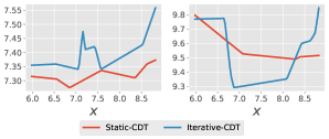
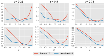
While using a static control approach can perform reasonably well in some situations, our results in Section 5 suggest that the iterative control procedure is a more reliable strategy. This is consistent with findings in the stochastic optimal control literature (Thijssen & Kappen, 2015; Pereira et al., 2019). This choice of control function drives the forward process 𝐗t𝐜,𝐲subscriptsuperscript𝐗𝐜𝐲𝑡\mathbf{X}^{\mathbf{c},\mathbf{y}}_{t} to regions of the state-space where the likelihood function is large and helps mitigate convergence and stability issues. Furthermore, Section 5 reports that (at convergence), the solutions N0subscript𝑁0N_{0} and N𝑁N can be significantly different. The iterative control procedure leads to more accurate solutions and, ultimately, better performance when used for online filtering.

3.3 Online filtering

Before performing online filtering, we first run the CDT algorithm described in Section 3.2 to construct an approximation of the optimal control 𝐜(𝐱,𝐲,t)=[σlogh](𝐱,𝐲,t)subscript𝐜𝐱𝐲𝑡delimited-[]superscript𝜎top𝐱𝐲𝑡\mathbf{c}_{\star}(\mathbf{x},\mathbf{y},t)=[\sigma^{\top}\nabla\log h](\mathbf{x},\mathbf{y},t). For concreteness, denote by 𝐜^:𝒳×𝒴×[0,T]d:^𝐜𝒳𝒴0𝑇superscript𝑑\widehat{\mathbf{c}}:\mathcal{X}\times\mathcal{Y}\times[0,T]\to\mathbb{R}^{d} the resulting approximate control, i.e. 𝐜^(𝐱,𝐲,t)=N(𝐱,𝐲,t)^𝐜𝐱𝐲𝑡𝑁𝐱𝐲𝑡\widehat{\mathbf{c}}(\mathbf{x},\mathbf{y},t)=-N(\mathbf{x},\mathbf{y},t) where N(,,)𝑁N(\cdot,\cdot,\cdot) is parametrized by the final parameter θΘ𝜃Θ\theta\in\Theta. Similarly, denote by V^0:𝒳×𝒴:subscript^𝑉0𝒳𝒴\widehat{V}_{0}:\mathcal{X}\times\mathcal{Y}\to\mathbb{R} the approximation of the initial value function v(𝐱,𝐲,0)=logh(𝐱,𝐲,0)𝑣𝐱𝐲0𝐱𝐲0v(\mathbf{x},\mathbf{y},0)=-\log h(\mathbf{x},\mathbf{y},0), i.e. V^0(𝐱,𝐲)=N0(𝐱,𝐲)subscript^𝑉0𝐱𝐲subscript𝑁0𝐱𝐲\widehat{V}_{0}(\mathbf{x},\mathbf{y})=N_{0}(\mathbf{x},\mathbf{y}) where N0(,)subscript𝑁0N_{0}(\cdot,\cdot) is parametrized by the final parameter θ0Θ0subscript𝜃0subscriptΘ0\theta_{0}\in\Theta_{0}.

For implementing online filtering with M1𝑀1M\geq 1 particles, consider a current approximation of the filtering distribution at time tk0subscript𝑡𝑘0t_{k}\geq 0, i.e. πk(d𝐱)M1j=1Mδ(d𝐱;𝐱tkj)subscript𝜋𝑘𝑑𝐱superscript𝑀1superscriptsubscript𝑗1𝑀𝛿𝑑𝐱subscriptsuperscript𝐱𝑗subscript𝑡𝑘\pi_{k}(d\mathbf{x})\approx M^{-1}\sum_{j=1}^{M}\delta(d\mathbf{x};\mathbf{x}^{j}_{t_{k}}). Given the future observation 𝐘k+1=𝐲k+1subscript𝐘𝑘1subscript𝐲𝑘1\mathbf{Y}_{{k+1}}=\mathbf{y}_{k+1}, the particles 𝐱tk1:Msubscriptsuperscript𝐱:1𝑀subscript𝑡𝑘\mathbf{x}^{1:M}_{t_{k}} are then propagated forward by exploiting the approximately optimal control (𝐱,t)𝐜^(𝐱,𝐲k+1,ttk)maps-to𝐱𝑡^𝐜𝐱subscript𝐲𝑘1𝑡subscript𝑡𝑘(\mathbf{x},t)\mapsto\widehat{\mathbf{c}}(\mathbf{x},\mathbf{y}_{k+1},t-t_{k}). In particular, 𝐱^tk+1jsubscriptsuperscript^𝐱𝑗subscript𝑡𝑘1\widehat{\mathbf{x}}^{j}_{t_{k+1}} is obtained by setting 𝐱^tk+1j=𝐗^tk+1jsubscriptsuperscript^𝐱𝑗subscript𝑡𝑘1subscriptsuperscript^𝐗𝑗subscript𝑡𝑘1\widehat{\mathbf{x}}^{j}_{t_{k+1}}=\widehat{\mathbf{X}}^{j}_{t_{k+1}} where {𝐗^tj}t[tk,tk+1]subscriptsubscriptsuperscript^𝐗𝑗𝑡𝑡subscript𝑡𝑘subscript𝑡𝑘1\{\widehat{\mathbf{X}}^{j}_{t}\}_{t\in[t_{k},t_{k+1}]} follows the controlled diffusion

d𝐗^tj=μ(𝐗^tj)dt+σ(𝐗^tj)d𝐁tj(original dynamics)+[σ𝐜^](𝐗^tj,𝐲k+1,ttk)dt(approximately optimal control)𝑑subscriptsuperscript^𝐗𝑗𝑡subscript𝜇subscriptsuperscript^𝐗𝑗𝑡𝑑𝑡𝜎subscriptsuperscript^𝐗𝑗𝑡𝑑subscriptsuperscript𝐁𝑗𝑡(original dynamics)subscriptdelimited-[]𝜎^𝐜subscriptsuperscript^𝐗𝑗𝑡subscript𝐲𝑘1𝑡subscript𝑡𝑘𝑑𝑡(approximately optimal control)\displaystyle d\widehat{\mathbf{X}}^{j}_{t}=\underbrace{\mu(\widehat{\mathbf{X}}^{j}_{t})\,dt+\sigma(\widehat{\mathbf{X}}^{j}_{t})\,d\mathbf{B}^{j}_{t}}_{\text{(original dynamics)}}+\underbrace{[\sigma\widehat{\mathbf{c}}](\widehat{\mathbf{X}}^{j}_{t},\mathbf{y}_{k+1},t-t_{k})\,dt}_{\text{(approximately optimal control)}} (14)

initialized at 𝐗^tkj=𝐱tkjsubscriptsuperscript^𝐗𝑗subscript𝑡𝑘subscriptsuperscript𝐱𝑗subscript𝑡𝑘\widehat{\mathbf{X}}^{j}_{t_{k}}=\mathbf{x}^{j}_{t_{k}}. Each propagated particle 𝐱^tk+1jsubscriptsuperscript^𝐱𝑗subscript𝑡𝑘1\widehat{\mathbf{x}}^{j}_{t_{k+1}} is associated with a normalized weight W¯k+1j=Wk+1j/i=1MWk+1isubscriptsuperscript¯𝑊𝑗𝑘1subscriptsuperscript𝑊𝑗𝑘1superscriptsubscript𝑖1𝑀subscriptsuperscript𝑊𝑖𝑘1\overline{W}^{j}_{k+1}=W^{j}_{k+1}/\sum_{i=1}^{M}W^{i}_{k+1} where Wk+1j=(d[tk,tk+1]/d[tk,tk+1]𝐜^,𝐲k+1)(𝐗^[tk,tk+1]j)×g(𝐱^tk+1j,𝐲k+1)subscriptsuperscript𝑊𝑗𝑘1𝑑subscriptsubscript𝑡𝑘subscript𝑡𝑘1𝑑subscriptsuperscript^𝐜subscript𝐲𝑘1subscript𝑡𝑘subscript𝑡𝑘1superscriptsubscript^𝐗subscript𝑡𝑘subscript𝑡𝑘1𝑗𝑔subscriptsuperscript^𝐱𝑗subscript𝑡𝑘1subscript𝐲𝑘1W^{j}_{k+1}=(d\mathbb{P}_{[t_{k},t_{k+1}]}/d\mathbb{P}^{\widehat{\mathbf{c}},\mathbf{y}_{k+1}}_{[t_{k},t_{k+1}]})(\widehat{\mathbf{X}}_{[t_{k},t_{k+1}]}^{j})\times g(\widehat{\mathbf{x}}^{j}_{t_{k+1}},\mathbf{y}_{k+1}). We recall that the probability measures [tk,tk+1]subscriptsubscript𝑡𝑘subscript𝑡𝑘1\mathbb{P}_{[t_{k},t_{k+1}]} and [tk,tk+1]𝐜^,𝐲k+1subscriptsuperscript^𝐜subscript𝐲𝑘1subscript𝑡𝑘subscript𝑡𝑘1\mathbb{P}^{\widehat{\mathbf{c}},\mathbf{y}_{k+1}}_{[t_{k},t_{k+1}]} correspond to the original and controlled diffusions on the interval [tk,tk+1]subscript𝑡𝑘subscript𝑡𝑘1[t_{k},t_{k+1}]. Girsanov’s theorem, as described in Section 2.3, implies that Wk+1jsubscriptsuperscript𝑊𝑗𝑘1W^{j}_{k+1} is

exp{12tktk+1𝐙tj2𝑑t+tktk+1𝐙tj,d𝐁tj}g(𝐱^tk+1j,𝐲k+1)12superscriptsubscriptsubscript𝑡𝑘subscript𝑡𝑘1superscriptnormsubscriptsuperscript𝐙𝑗𝑡2differential-d𝑡superscriptsubscriptsubscript𝑡𝑘subscript𝑡𝑘1subscriptsuperscript𝐙𝑗𝑡𝑑subscriptsuperscript𝐁𝑗𝑡𝑔subscriptsuperscript^𝐱𝑗subscript𝑡𝑘1subscript𝐲𝑘1\displaystyle\exp{\left\{-\frac{1}{2}\int_{t_{k}}^{t_{k+1}}\|\mathbf{Z}^{j}_{t}\|^{2}\,dt+\int_{t_{k}}^{t_{k+1}}\langle\mathbf{Z}^{j}_{t},d\mathbf{B}^{j}_{t}\rangle\right\}}g(\widehat{\mathbf{x}}^{j}_{t_{k+1}},\mathbf{y}_{k+1})

where 𝐙tj=𝐜^(𝐗^tj,𝐲k+1,ttk)subscriptsuperscript𝐙𝑗𝑡^𝐜subscriptsuperscript^𝐗𝑗𝑡subscript𝐲𝑘1𝑡subscript𝑡𝑘\mathbf{Z}^{j}_{t}=-\widehat{\mathbf{c}}(\widehat{\mathbf{X}}^{j}_{t},\mathbf{y}_{k+1},t-t_{k}). Similarly to Equation (9), consider the diffusion process {Vtj}t[tk,tk+1]subscriptsubscriptsuperscript𝑉𝑗𝑡𝑡subscript𝑡𝑘subscript𝑡𝑘1\{V^{j}_{t}\}_{t\in[t_{k},t_{k+1}]} defined by the dynamics

dVtj=12𝐙tj2dt+𝐙tj,d𝐁tj𝑑subscriptsuperscript𝑉𝑗𝑡12superscriptnormsubscriptsuperscript𝐙𝑗𝑡2𝑑𝑡subscriptsuperscript𝐙𝑗𝑡𝑑subscriptsuperscript𝐁𝑗𝑡\displaystyle dV^{j}_{t}=-\frac{1}{2}\|\mathbf{Z}^{j}_{t}\|^{2}\,dt+\langle\mathbf{Z}^{j}_{t},d\mathbf{B}^{j}_{t}\rangle (15)

with initialization at Vtkj=V^0(𝐱tkj,𝐲k+1)subscriptsuperscript𝑉𝑗subscript𝑡𝑘subscript^𝑉0subscriptsuperscript𝐱𝑗subscript𝑡𝑘subscript𝐲𝑘1V^{j}_{t_{k}}=\widehat{V}_{0}(\mathbf{x}^{j}_{t_{k}},\mathbf{y}_{k+1}). Therefore the weight Wk+1jsubscriptsuperscript𝑊𝑗𝑘1W^{j}_{k+1} can be re-written as

exp{Vtk+1j+logg(𝐱^tk+1j,𝐲k+1)0V^0(𝐱tkj,𝐲k+1)},subscriptsubscriptsuperscript𝑉𝑗subscript𝑡𝑘1𝑔subscriptsuperscript^𝐱𝑗subscript𝑡𝑘1subscript𝐲𝑘1absent0subscript^𝑉0subscriptsuperscript𝐱𝑗subscript𝑡𝑘subscript𝐲𝑘1\displaystyle\exp\Big{\{}\underbrace{V^{j}_{t_{k+1}}+\log g(\widehat{\mathbf{x}}^{j}_{t_{k+1}},\mathbf{y}_{k+1})}_{\approx 0}-\widehat{V}_{0}(\mathbf{x}^{j}_{t_{k}},\mathbf{y}_{k+1})\Big{\}}, (16)

and computed by numerically integrating the process {Vtj}t[tk,tk+1]subscriptsubscriptsuperscript𝑉𝑗𝑡𝑡subscript𝑡𝑘subscript𝑡𝑘1\{V^{j}_{t}\}_{t\in[t_{k},t_{k+1}]}. Given the definition of the loss function in (12), we can expect the sum of the first two terms within the exponential to be close to zero. In the ideal case where 𝐜^(𝐱,𝐲,t)𝐜(𝐱,𝐲,t)^𝐜𝐱𝐲𝑡subscript𝐜𝐱𝐲𝑡\widehat{\mathbf{c}}(\mathbf{x},\mathbf{y},t)\equiv\mathbf{c}_{\star}(\mathbf{x},\mathbf{y},t) and V^0(𝐱,𝐲)logh(𝐱,𝐲,0)subscript^𝑉0𝐱𝐲𝐱𝐲0\widehat{V}_{0}(\mathbf{x},\mathbf{y})\equiv-\log h(\mathbf{x},\mathbf{y},0), one recovers the exact AF-APF weights in (3). Once the above weights are computed, the resampling steps are identical to those described in Section 2.2 for a standard PF. For practical implementations, all the processes involved in the proposed methodology can be straightforwardly time-discretized. To distinguish between CDT learning with static or iterative control, we shall refer to the resulting approximation of FA-APF as Static-APF and Iterative-APF respectively. We note that these APFs do not involve modified resampling probabilities as described e.g. in Chopin et al. (2020, p. 145).

Auxiliary particle filter.

We end this section by summarizing the steps required to assimilate a future observation 𝐘k+1=𝐲k+1subscript𝐘𝑘1subscript𝐲𝑘1\mathbf{Y}_{{k+1}}=\mathbf{y}_{k+1} at time tk+1subscript𝑡𝑘1t_{k+1} using our proposed APF.

  1. 1.

    Suppose we have an equally weighted set of particles 𝐱tk1:Msubscriptsuperscript𝐱:1𝑀subscript𝑡𝑘\mathbf{x}^{1:M}_{t_{k}} approximating of the filtering distribution at time tksubscript𝑡𝑘t_{k}.

  2. 2.

    Generate the controlled trajectories: the j𝑗j-th sample path 𝐗^[tk,tk+1]jsubscriptsuperscript^𝐗𝑗subscript𝑡𝑘subscript𝑡𝑘1\widehat{\mathbf{X}}^{j}_{[t_{k},t_{k+1}]} is obtained by forward integration of the controlled dynamics in Equation (14) with initial condition 𝐗^tkj=𝐱tkjsubscriptsuperscript^𝐗𝑗subscript𝑡𝑘subscriptsuperscript𝐱𝑗subscript𝑡𝑘\widehat{\mathbf{X}}^{j}_{t_{k}}=\mathbf{x}^{j}_{t_{k}}, control 𝐜^(,𝐲k+1,ttk)^𝐜subscript𝐲𝑘1𝑡subscript𝑡𝑘\widehat{\mathbf{c}}(\cdot,\mathbf{y}_{k+1},t-t_{k}), and the Brownian path 𝐁[tk,tk+1]jsubscriptsuperscript𝐁𝑗subscript𝑡𝑘subscript𝑡𝑘1\mathbf{B}^{j}_{[t_{k},t_{k+1}]}. Set next particle as 𝐱^tk+1j=𝐗^tk+1jsubscriptsuperscript^𝐱𝑗subscript𝑡𝑘1subscriptsuperscript^𝐗𝑗subscript𝑡𝑘1\widehat{\mathbf{x}}^{j}_{t_{k+1}}=\widehat{\mathbf{X}}^{j}_{t_{k+1}}.

  3. 3.

    Generate the value trajectories: the j𝑗j-th sample path V[tk,tk+1]jsubscriptsuperscript𝑉𝑗subscript𝑡𝑘subscript𝑡𝑘1V^{j}_{[t_{k},t_{k+1}]} is obtained by forward integration of the dynamics in Equation (15) with initial condition Vtkj=V^0(𝐱tkj,𝐲k+1)subscriptsuperscript𝑉𝑗subscript𝑡𝑘subscript^𝑉0subscriptsuperscript𝐱𝑗subscript𝑡𝑘subscript𝐲𝑘1V^{j}_{t_{k}}=\widehat{V}_{0}(\mathbf{x}^{j}_{t_{k}},\mathbf{y}_{k+1}), control 𝐙tj=𝐜^(𝐗^tj,𝐲k+1,ttk)subscriptsuperscript𝐙𝑗𝑡^𝐜subscriptsuperscript^𝐗𝑗𝑡subscript𝐲𝑘1𝑡subscript𝑡𝑘\mathbf{Z}^{j}_{t}=-\widehat{\mathbf{c}}(\widehat{\mathbf{X}}^{j}_{t},\mathbf{y}_{k+1},t-t_{k}), and the Brownian path 𝐁[tk,tk+1]jsubscriptsuperscript𝐁𝑗subscript𝑡𝑘subscript𝑡𝑘1\mathbf{B}^{j}_{[t_{k},t_{k+1}]}.

  4. 4.

    Compute weight Wk+1jsuperscriptsubscript𝑊𝑘1𝑗W_{k+1}^{j} using (16) and normalize weight W¯k+1j=Wk+1j/i=1MWk+1isubscriptsuperscript¯𝑊𝑗𝑘1subscriptsuperscript𝑊𝑗𝑘1superscriptsubscript𝑖1𝑀subscriptsuperscript𝑊𝑖𝑘1\overline{W}^{j}_{{k+1}}=W^{j}_{{k+1}}/\sum_{i=1}^{M}W^{i}_{{k+1}}.

  5. 5.

    Obtain new set of equally weighted particles 𝐱tk+11:Msubscriptsuperscript𝐱:1𝑀subscript𝑡𝑘1\mathbf{x}^{1:M}_{t_{k+1}} approximating the filtering distribution at time tk+1subscript𝑡𝑘1t_{k+1} by resampling 𝐱^tk+11:Msubscriptsuperscript^𝐱:1𝑀subscript𝑡𝑘1\widehat{\mathbf{x}}^{1:M}_{t_{k+1}} with probabilities W¯k+11:Msubscriptsuperscript¯𝑊:1𝑀𝑘1\overline{W}^{1:M}_{{k+1}}.

4 Related work

This section positions our work within the existing literature.

MCMC methods: Several works have developed Markov Chain Monte Carlo (MCMC) methods for smoothing and parameter estimation of SDEs; for example, Roberts & Stramer (2001) proposes to treat paths between observations as missing data. Our work focuses on the online filtering problem which cannot be tackled with MCMC methods.

Exact simulation: Several methods have been proposed to reduce or eliminate the bias due to time-discretization (Beskos et al., 2006a, b; Fearnhead et al., 2010, 2008; Jasra et al., 2022). Most of these methods rely on the Lamperti transform which is typically impossible in multivariate settings. In contrast, our method does not exploit any specific structure of the diffusion process being assimilated. Furthermore, when filtering diffusions with highly informative observations, the discretization bias is often orders of magnitude smaller than other sources of errors.

Gaussian assumptions: In the data assimilation literature, methods based on variations of the Ensemble Kalman Filter (EnKF) (Evensen, 2003) have been successfully deployed in applications with very high dimensions. These methods strongly rely on underlying Gaussian assumptions and can give very poor results for highly nonlinear and non-Gaussian models. In contrast, our method is asymptotically exact in the limit when the number of particles M𝑀M\to\infty (up to discretization error). Indeed, we do not expect our method to be competitive relative to this class of (approximate) methods in very high dimensional settings that are common in numerical weather forecasting. These methods typically achieve lower variance at the cost of larger bias that is hard to estimate. Our method is designed to filter diffusion processes in low or moderate dimensional settings. It is likely that scaling our method to truly high dimensional settings would require introducing model-specific approximations (e.g. localization strategies).

Steering particles towards observations: particle methods pioneered by Van Leeuwen (2010) are based on this intuitive idea in order to mitigate collapse of PFs in high dimensional settings found in applications such as geoscience. These methods typically rely on some model structure (e.g. linear Gaussian observation model) and have a number of tuning parameters. They can be understood as parameterizing a linear control, which is only expected to work well for problems with linear Gaussian dynamics.

Implicit Particle Filter: the method of Chorin et al. (2010) attempts to transform standard Gaussian samples into samples from the (locally) optimal proposal density. Implementing this methodology requires a number of assumptions and requires solving a non-convex optimization step for each particle and each time step, which can be computationally burdensome.

Guided Intermediate Resampling Filters (GIRF): the method of Del Moral & Murray (2015) and Park & Ionides (2020) propagates particles at intermediate time intervals between observations with the original dynamics and triggers resampling steps based on a guiding functions that forecast the likelihood of future observations. The choice of guiding functions is crucial for good algorithmic performance. We note that GIRF is in fact intimately related to Doob’s hh-transform as the optimal choice of guiding functions is given by (5) (Park & Ionides, 2020). However, even under this optimal choice, the resulting GIRF is still sub-optimal when compared to an APF that moves particles using the optimal control induced by Doob’s hh-transform, i.e. it is better to move particles well rather than rely on weighting and resampling. The latter behaviour is supported by our numerical experiments. Appendix C details our GIRF implementation and the connection to Doob’s hh-transform.

5 Experiments

This section presents numerical results obtained on three models. All experiments employed 200020002000 iterations of the Adam optimizer with a learning rate of 0.010.010.01 and a mini-batch size of 100010001000 sample paths with 101010 different observations and 100100100 paths associated to each observation. Appendix D describes how the CDT algorithm and neural network approximations behave during training. Training times took around one to two minutes on a standard CPU: it is negligible when compared to the cost of running filters with many particles and/or to assimilate large number of observations. The inter-observation time was T=1𝑇1T=1 and we employed the Euler–Maruyama integrator with a stepsize of 0.020.020.02 for all examples. Our results are not sensitive to the choice of T𝑇T and discretization stepsize as long as it is sufficiently small. We report the Effective Sample Size (ESS) averaged over observation times and independent repetitions,111As GIRF involves intermediate time steps between observation times, its effective sample size is not comparable to the other particle filters and hence not reported. the evidence lower bound (ELBO) 𝔼[logp^(𝐲1,,𝐲K)]𝔼delimited-[]^𝑝subscript𝐲1subscript𝐲𝐾\mathbb{E}[\log\widehat{p}(\mathbf{y}_{1},\ldots,\mathbf{y}_{K})], and the variance Var[logp^(𝐲1,,𝐲K)]Vardelimited-[]^𝑝subscript𝐲1subscript𝐲𝐾\textrm{Var}[\log\widehat{p}(\mathbf{y}_{1},\ldots,\mathbf{y}_{K})], where p^(𝐲1,,𝐲K)^𝑝subscript𝐲1subscript𝐲𝐾\widehat{p}(\mathbf{y}_{1},\ldots,\mathbf{y}_{K}) denotes its unbiased estimator of the marginal likelihood of the time-discretized filter p(𝐲1,,𝐲K)𝑝subscript𝐲1subscript𝐲𝐾p(\mathbf{y}_{1},\ldots,\mathbf{y}_{K}). When testing particle filters with varying number of observations K𝐾K, we increased the number of particles M𝑀M linearly with K𝐾K to keep marginal likelihood estimators stable (Bérard et al., 2014). For non-toy models, our GIRF implementation relies on a sub-optimal but practical choice of guiding functions that gradually introduce information from the future observation by annealing the observation density using a linear (Linear-GIRF) or quadratic schedule (Quadratic-GIRF).

5.1 Ornstein–Uhlenbeck model

Consider a d𝑑d-dimensional Ornstein–Uhlenbeck process given by (1) with μ(𝐱)=𝐱𝜇𝐱𝐱\mu(\mathbf{x})=-\mathbf{x}, σ(𝐱)=𝐈d𝜎𝐱subscript𝐈𝑑\sigma(\mathbf{x})=\mathbf{I}_{d} and the Gaussian observation model g(𝐱,𝐲)=𝒩(𝐲;𝐱,σ𝐘2𝐈d)𝑔𝐱𝐲𝒩𝐲𝐱superscriptsubscript𝜎𝐘2subscript𝐈𝑑g(\mathbf{x},\mathbf{y})=\mathcal{N}(\mathbf{y};\mathbf{x},\sigma_{\mathbf{Y}}^{2}\mathbf{I}_{d}). We chose η𝐗=𝒩(𝟎d,𝐈d/2)subscript𝜂𝐗𝒩subscript0𝑑subscript𝐈𝑑2\eta_{\mathbf{X}}=\mathcal{N}(\mathbf{0}_{d},\mathbf{I}_{d}/2) as the stationary distribution and η𝐘=𝒩(𝟎d,(1/2+σ𝐘2)𝐈d)subscript𝜂𝐘𝒩subscript0𝑑12superscriptsubscript𝜎𝐘2subscript𝐈𝑑\eta_{\mathbf{Y}}=\mathcal{N}(\mathbf{0}_{d},(1/2+\sigma_{\mathbf{Y}}^{2})\mathbf{I}_{d}) as the implied distribution of the observation when training neural networks with the CDT iterative scheme. We took different values of σ𝐘{0.125,0.25,0.5,1.0}subscript𝜎𝐘0.1250.250.51.0\sigma_{\mathbf{Y}}\in\{0.125,0.25,0.5,1.0\} to vary the informativeness of observations and d{1,2,4,8,16,32}𝑑12481632d\in\{1,2,4,8,16,32\} to illustrate the impact of dimension.

Analytical tractability in this example (Appendix B) allows us to consider three idealized particle filters, namely an APF with exact networks (Exact-APF), FA-APF, and GIRF with optimal guiding functions (Appendix C). Comparing our proposed Iterative-APF to Exact-APF and FA-APF enables us to distinguish between neural network approximation errors and time-discretization errors. We note that all PFs except the FA-APF involve time-discretization.

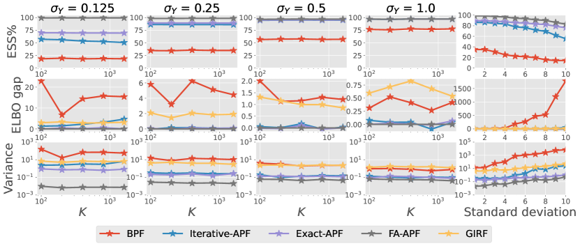
Columns 111 to 444 of Figure 2 summarize our numerical findings when filtering simulated observations from the model with varying σ𝐘subscript𝜎𝐘\sigma_{\mathbf{Y}} and fixed d=1𝑑1d=1. We see that the performance of BPF deteriorates as the observations become more informative, which is to be expected. Furthermore, when σ𝐘subscript𝜎𝐘\sigma_{\mathbf{Y}} is small, the impact of our neural network approximation and time-discretization becomes more noticeable. For the values of σ𝐘subscript𝜎𝐘\sigma_{\mathbf{Y}} and the number of observations K𝐾K considered, Iterative-APF had substantial gains in efficiency over BPF and typically outperformed GIRF. From Column 5, we note that these gains over BPF become very large when we filter K=100𝐾100K=100 observations simulated with observation standard deviations that are multiples of σ𝐘=0.25subscript𝜎𝐘0.25\sigma_{\mathbf{Y}}=0.25 which was used to run the filters. In particular, while the ELBO of BPF diverges as we increase the degree of noise in the simulated observations, the ELBO of Iterative-APF and GIRF remain stable.

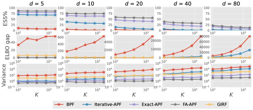
Figure 3 shows the impact of increasing dimension d𝑑d with fixed σ𝐘=0.5subscript𝜎𝐘0.5\sigma_{\mathbf{Y}}=0.5 when filtering simulated observations from the model. We note that it computationally infeasible to consider classical PDE solvers in dimension d>4𝑑4d>4. Due to the curse of dimensionality, it is not surprising for the performance of all PFs to degrade with dimension (Snyder et al., 2008, 2015). Although the error of our neural network approximation becomes more pronounced when d𝑑d is large, the gain in efficiency of Iterative-APF relative to BPF is very significant in the higher dimensional regime, and particularly so when the number of observations K𝐾K is also large. As dimension increases, we see that the performance of the practical Iterative-APF decreases compared to an idealized implementation of GIRF. However, GIRF was still outperformed by the idealized Exact-APF for all dimensions d𝑑d considered, verifying that it is indeed more beneficial to move particles well instead of using weighting and resampling mechanisms.
Refer to caption

Figure 2: Results for Ornstein–Uhlenbeck model with d=1𝑑1d=1 based on 100100100 independent repetitions of each PF. The ELBO gap in the second row is relative to FA-APF.

Refer to caption

Figure 3: Results for Ornstein–Uhlenbeck model with σ𝐘=0.5subscript𝜎𝐘0.5\sigma_{\mathbf{Y}}=0.5 based on 100100100 independent repetitions of each PF. The ELBO gap in the second row is relative to FA-APF.

5.2 Logistic diffusion model

Next we consider a logistic diffusion process (Dennis & Costantino, 1988; Knape & De Valpine, 2012) to model the dynamics of a population size {𝐏t}t0subscriptsubscript𝐏𝑡𝑡0\{\mathbf{P}_{t}\}_{t\geq 0}, defined by

d𝐏t=(θ32/2+θ1θ2𝐏t)𝐏tdt+θ3𝐏td𝐁t.𝑑subscript𝐏𝑡superscriptsubscript𝜃322subscript𝜃1subscript𝜃2subscript𝐏𝑡subscript𝐏𝑡𝑑𝑡subscript𝜃3subscript𝐏𝑡𝑑subscript𝐁𝑡\displaystyle d\mathbf{P}_{t}=(\theta_{3}^{2}/2+\theta_{1}-\theta_{2}\mathbf{P}_{t})\mathbf{P}_{t}\,dt+\theta_{3}\mathbf{P}_{t}\,d\mathbf{B}_{t}. (17)

We apply the Lamperti transformation 𝐗t=log(𝐏t)/θ3subscript𝐗𝑡subscript𝐏𝑡subscript𝜃3\mathbf{X}_{t}=\log(\mathbf{P}_{t})/\theta_{3} and work with the process {𝐗t}t0subscriptsubscript𝐗𝑡𝑡0\{\mathbf{X}_{t}\}_{t\geq 0} that satisfies (1) with μ(𝐱)=θ1/θ3(θ2/θ3)exp(θ3𝐱)𝜇𝐱subscript𝜃1subscript𝜃3subscript𝜃2subscript𝜃3subscript𝜃3𝐱\mu(\mathbf{x})=\theta_{1}/\theta_{3}-(\theta_{2}/\theta_{3})\exp(\theta_{3}\mathbf{x}) and σ(𝐱)=1𝜎𝐱1\sigma(\mathbf{x})=1. Following (Knape & De Valpine, 2012), we adopt a negative binomial observation model g(𝐱,𝐲)=𝒩(𝐲;θ4,exp(θ3𝐱))𝑔𝐱𝐲𝒩𝐲subscript𝜃4subscript𝜃3𝐱g(\mathbf{x},\mathbf{y})=\mathcal{NB}(\mathbf{y};\theta_{4},\exp(\theta_{3}\mathbf{x})) for counts 𝐲0𝐲subscript0\mathbf{y}\in\mathbb{N}_{0} with dispersion θ4>0subscript𝜃40\theta_{4}>0 and mean exp(θ3𝐱)subscript𝜃3𝐱\exp(\theta_{3}\mathbf{x}). We set (θ1,θ2,θ3,θ4)subscript𝜃1subscript𝜃2subscript𝜃3subscript𝜃4(\theta_{1},\theta_{2},\theta_{3},\theta_{4}) as the parameter estimates obtained in (Knape & De Valpine, 2012). Noting that (17) admits a Gamma distribution with shape parameter 2(θ32/2+θ1)/θ3212superscriptsubscript𝜃322subscript𝜃1superscriptsubscript𝜃3212(\theta_{3}^{2}/2+\theta_{1})/\theta_{3}^{2}-1 and rate parameter 2θ2/θ322subscript𝜃2superscriptsubscript𝜃322\theta_{2}/\theta_{3}^{2} as stationary distribution (Dennis & Costantino, 1988), we select η𝐗subscript𝜂𝐗\eta_{\mathbf{X}} as the push-forward under the Lamperti transformation and η𝐘subscript𝜂𝐘\eta_{\mathbf{Y}} as the implied distribution of the observation when training neural networks under both static and iterative CDT schemes. To induce varying levels of informative observations, we considered θ4{1.069,4.303,17.631,78.161}subscript𝜃41.0694.30317.63178.161\theta_{4}\in\{1.069,4.303,17.631,78.161\}.

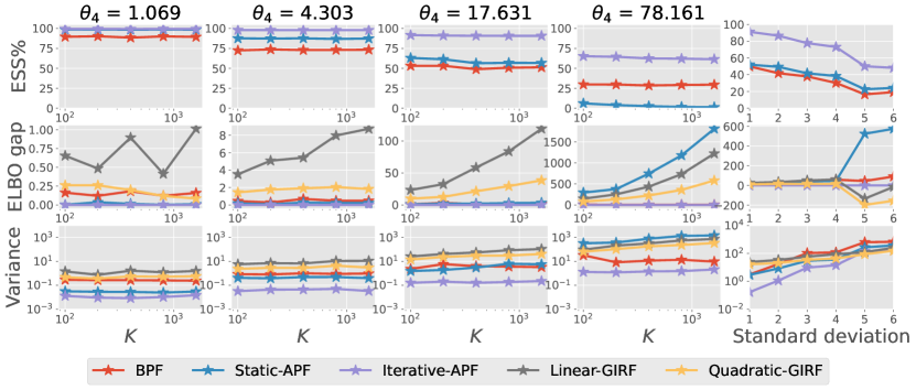
Figure 4 displays our filtering results for various number of simulated observations from the model (Columns 111 to 444) and for K=100𝐾100K=100 observations that are simulated with observation standard deviations larger than θ4=17.631subscript𝜃417.631\theta_{4}=17.631 used to run the filters (Column 5). In the latter setup, we solved for different values of θ4subscript𝜃4\theta_{4} in the negative binomial observation model to induce larger standard deviations. The behaviour of BPF and Iterative-APF is similar to the previous example as the observations become more informative with larger values of θ4subscript𝜃4\theta_{4}. Iterative-APF outperformed all other algorithms over all combinations of θ4subscript𝜃4\theta_{4} and K𝐾K considered, and also when filtering observations that are increasingly extreme under the model. We note also that the APFs trained using the CDT static scheme can sometimes give unstable results, particularly in challenging scenarios.
Refer to caption

Figure 4: Results for logistic diffusion model based on 100100100 independent repetitions of each PF. The ELBO gap in the second row is relative to Iterative-APF.

5.3 Cell model

Lastly we examine a cell differentiation and development model from (Wang et al., 2011). Cellular expression levels 𝐗t=(𝐗t,1,𝐗t,2)subscript𝐗𝑡subscript𝐗𝑡1subscript𝐗𝑡2\mathbf{X}_{t}=(\mathbf{X}_{t,1},\mathbf{X}_{t,2}) of two genes are modelled by (1) with

μ(𝐱)=(𝐱14/(24+𝐱14)+24/(24+𝐱24)𝐱1𝐱24/(24+𝐱24)+24/(24+𝐱14)𝐱2)𝜇𝐱matrixsuperscriptsubscript𝐱14superscript24superscriptsubscript𝐱14superscript24superscript24superscriptsubscript𝐱24subscript𝐱1superscriptsubscript𝐱24superscript24superscriptsubscript𝐱24superscript24superscript24superscriptsubscript𝐱14subscript𝐱2\displaystyle\mu(\mathbf{x})=\begin{pmatrix}\mathbf{x}_{1}^{4}/(2^{-4}+\mathbf{x}_{1}^{4})+2^{-4}/(2^{-4}+\mathbf{x}_{2}^{4})-\mathbf{x}_{1}\\ \mathbf{x}_{2}^{4}/(2^{-4}+\mathbf{x}_{2}^{4})+2^{-4}/(2^{-4}+\mathbf{x}_{1}^{4})-\mathbf{x}_{2}\end{pmatrix}

and σ(𝐱)=0.1𝐈d𝜎𝐱0.1subscript𝐈𝑑\sigma(\mathbf{x})=\sqrt{0.1}\mathbf{I}_{d}. The above terms describe self-activation, mutual inhibition, and inactivation respectively, and the volatility captures intrinsic and external fluctuations. We initialize the diffusion process from the undifferentiated state of 𝐗0=(1,1)subscript𝐗011\mathbf{X}_{0}=(1,1) and consider the Gaussian observation model g(𝐱,𝐲)=𝒩(𝐲;𝐱,σ𝐘2𝐈2)𝑔𝐱𝐲𝒩𝐲𝐱superscriptsubscript𝜎𝐘2subscript𝐈2g(\mathbf{x},\mathbf{y})=\mathcal{N}(\mathbf{y};\mathbf{x},\sigma_{\mathbf{Y}}^{2}\mathbf{I}_{2}). To train neural networks under both static and iterative CDT schemes, we selected η𝐗subscript𝜂𝐗\eta_{\mathbf{X}} and η𝐘subscript𝜂𝐘\eta_{\mathbf{Y}} as the empirical distributions obtained by simulating states and observations from the model for 200020002000 time units.

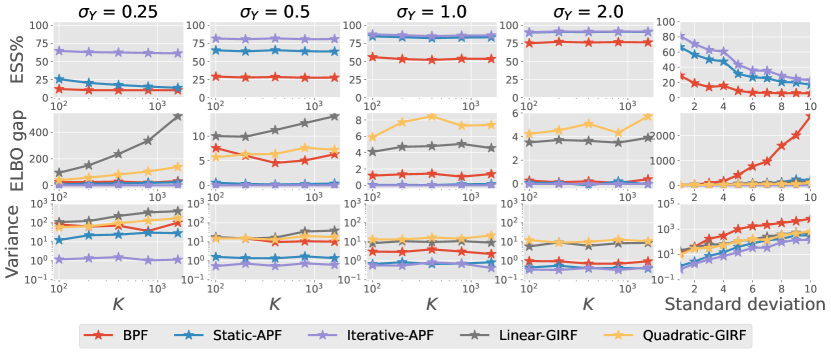
Figure 5 illustrates our numerical results for various number of observations K𝐾K and σ𝐘{0.25,0.5,1.0,2.0}subscript𝜎𝐘0.250.51.02.0\sigma_{\mathbf{Y}}\in\{0.25,0.5,1.0,2.0\}. It shows that Iterative-APF offers significant gains over all other algorithms when filtering observations that are informative (see Columns 111 to 444) and highly extreme under the model specification of σ𝐘=0.5subscript𝜎𝐘0.5\sigma_{\mathbf{Y}}=0.5 (see Column 5). In this example, Static-APF did not exhibit any unstable behaviour and its performance lies somewhere in between BPF and Iterative-APF.
Refer to caption

Figure 5: Results for cell model based on 100100100 independent repetitions of each PF. The ELBO gap in the second row is relative to Iterative-APF.

6 Discussion

This paper introduced the CDT algorithm to train particle filters for online filtering of diffusion processes evolving in state-spaces of low to moderate dimensions. Contrarily to a number of existing methods, the CDT approach is general and does not exploit any particular structure of the diffusion process and observation model. Furthermore, numerical simulations suggests that the CDT algorithm is particularly compelling in higher dimensional settings or in regimes when the observations are highly informative or extreme under the model specification. Ongoing work involves extending the CDT framework to parameter estimation and experimenting with alternative formulations and/or parameterizations to accelerate the training procedure. Finally, it is worth mentioning that although it is relatively straightforward to extend the proposed method to tackle unequal inter-observation intervals, we have not been able to use the same framework to deal with general time-dependent drift or volatility functions; this important problem is left for further investigations.

References

  • Allen (2010) Allen, L. J. An introduction to stochastic processes with applications to biology. CRC press, 2010.
  • Beck et al. (2019) Beck, C., E, W., and Jentzen, A. Machine learning approximation algorithms for high-dimensional fully nonlinear partial differential equations and second-order backward stochastic differential equations. Journal of Nonlinear Science, 29(4):1563–1619, 2019.
  • Bérard et al. (2014) Bérard, J., Del Moral, P., and Doucet, A. A lognormal central limit theorem for particle approximations of normalizing constants. Electronic Journal of Probability, 19:1–28, 2014.
  • Beskos et al. (2006a) Beskos, A., Papaspiliopoulos, O., and Roberts, G. O. Retrospective exact simulation of diffusion sample paths with applications. Bernoulli, 12(6):1077–1098, 2006a.
  • Beskos et al. (2006b) Beskos, A., Papaspiliopoulos, O., Roberts, G. O., and Fearnhead, P. Exact and computationally efficient likelihood-based estimation for discretely observed diffusion processes (with discussion). Journal of the Royal Statistical Society: Series B (Statistical Methodology), 68(3):333–382, 2006b.
  • Capasso & Capasso (2021) Capasso, V. and Capasso, V. Introduction to Continuous-Time Stochastic Processes. Springer, 2021.
  • Chan-Wai-Nam et al. (2019) Chan-Wai-Nam, Q., Mikael, J., and Warin, X. Machine learning for semi linear PDEs. Journal of Scientific Computing, 79(3):1667–1712, 2019.
  • Chopin et al. (2020) Chopin, N., Papaspiliopoulos, O., et al. An introduction to sequential Monte Carlo. Springer, 2020.
  • Chorin et al. (2010) Chorin, A., Morzfeld, M., and Tu, X. Implicit particle filters for data assimilation. Communications in Applied Mathematics and Computational Science, 5(2):221–240, 2010.
  • Chung & Walsh (2006) Chung, K. L. and Walsh, J. B. Markov processes, Brownian motion, and time symmetry, volume 249. Springer Science & Business Media, 2006.
  • Dai Pra (1991) Dai Pra, P. A stochastic control approach to reciprocal diffusion processes. Applied mathematics and Optimization, 23(1):313–329, 1991.
  • Del Moral (2004) Del Moral, P. Feynman-Kac formulae: genealogical and interacting particle systems with applications, volume 88. Springer, 2004.
  • Del Moral & Murray (2015) Del Moral, P. and Murray, L. M. Sequential Monte Carlo with highly informative observations. SIAM/ASA Journal on Uncertainty Quantification, 3(1):969–997, 2015.
  • Dennis & Costantino (1988) Dennis, B. and Costantino, R. F. Analysis of steady-state populations with the gamma abundance model: application to Tribolium. Ecology, 69(4):1200–1213, 1988.
  • Doucet et al. (2000) Doucet, A., Godsill, S., and Andrieu, C. On sequential monte carlo sampling methods for bayesian filtering. Statistics and computing, 10(3):197–208, 2000.
  • E et al. (2017) E, W., Han, J., and Jentzen, A. Deep learning-based numerical methods for high-dimensional parabolic partial differential equations and backward stochastic differential equations. Communications in Mathematics and Statistics, 5(4):349–380, 2017.
  • Evensen (2003) Evensen, G. The ensemble kalman filter: Theoretical formulation and practical implementation. Ocean dynamics, 53(4):343–367, 2003.
  • Fearnhead et al. (2008) Fearnhead, P., Papaspiliopoulos, O., and Roberts, G. O. Particle filters for partially observed diffusions. Journal of the Royal Statistical Society: Series B (Statistical Methodology), 70(4):755–777, 2008.
  • Fearnhead et al. (2010) Fearnhead, P., Papaspiliopoulos, O., Roberts, G. O., and Stuart, A. Random-weight particle filtering of continuous time processes. Journal of the Royal Statistical Society: Series B (Statistical Methodology), 72(4):497–512, 2010.
  • Gerber et al. (2019) Gerber, M., Chopin, N., and Whiteley, N. Negative association, ordering and convergence of resampling methods. The Annals of Statistics, 47(4):2236–2260, 2019.
  • Han et al. (2018) Han, J., Jentzen, A., and E, W. Solving high-dimensional partial differential equations using deep learning. Proceedings of the National Academy of Sciences, 115(34):8505–8510, 2018.
  • Hartmann et al. (2017) Hartmann, C., Richter, L., Schütte, C., and Zhang, W. Variational characterization of free energy: Theory and algorithms. Entropy, 19(11):626, 2017.
  • Hartmann et al. (2019) Hartmann, C., Kebiri, O., Neureither, L., and Richter, L. Variational approach to rare event simulation using least-squares regression. Chaos: An Interdisciplinary Journal of Nonlinear Science, 29(6):063107, 2019.
  • Huré et al. (2020) Huré, C., Pham, H., and Warin, X. Deep backward schemes for high-dimensional nonlinear PDEs. Mathematics of Computation, 89(324):1547–1579, 2020.
  • Hutzenthaler & Kruse (2020) Hutzenthaler, M. and Kruse, T. Multilevel Picard approximations of high-dimensional semilinear parabolic differential equations with gradient-dependent nonlinearities. SIAM Journal on Numerical Analysis, 58(2):929–961, 2020.
  • Hutzenthaler et al. (2020) Hutzenthaler, M., Jentzen, A., Kruse, T., Anh Nguyen, T., and von Wurstemberger, P. Overcoming the curse of dimensionality in the numerical approximation of semilinear parabolic partial differential equations. Proceedings of the Royal Society A, 476(2244):20190630, 2020.
  • Jasra et al. (2022) Jasra, A., Law, K. J., and Yu, F. Unbiased filtering of a class of partially observed diffusions. Advances in Applied Probability, 54(3):661–687, 2022.
  • Kebiri et al. (2017) Kebiri, O., Neureither, L., and Hartmann, C. Adaptive importance sampling with forward-backward stochastic differential equations. In International workshop on Stochastic Dynamics out of Equilibrium, pp.  265–281. Springer, 2017.
  • Kloeden & Platen (1992) Kloeden, P. E. and Platen, E. Stochastic differential equations. In Numerical Solution of Stochastic Differential Equations, pp.  103–160. Springer, 1992.
  • Knape & De Valpine (2012) Knape, J. and De Valpine, P. Fitting complex population models by combining particle filters with Markov chain Monte Carlo. Ecology, 93(2):256–263, 2012.
  • Nüsken & Richter (2021) Nüsken, N. and Richter, L. Solving high-dimensional Hamilton–Jacobi–Bellman PDEs using neural networks: perspectives from the theory of controlled diffusions and measures on path space. Partial Differential Equations and Applications, 2(4):1–48, 2021.
  • Oksendal (2013) Oksendal, B. Stochastic differential equations: an introduction with applications. Springer Science & Business Media, 2013.
  • Pardoux & Peng (1990) Pardoux, E. and Peng, S. Adapted solution of a backward stochastic differential equation. Systems & Control Letters, 14(1):55–61, 1990.
  • Pardoux & Peng (1992) Pardoux, E. and Peng, S. Backward stochastic differential equations and quasilinear parabolic partial differential equations. In Stochastic partial differential equations and their applications, pp.  200–217. Springer, 1992.
  • Pardoux & Tang (1999) Pardoux, E. and Tang, S. Forward-backward stochastic differential equations and quasilinear parabolic PDEs. Probability Theory and Related Fields, 114(2):123–150, 1999.
  • Park & Ionides (2020) Park, J. and Ionides, E. L. Inference on high-dimensional implicit dynamic models using a guided intermediate resampling filter. Statistics and Computing, 30(5):1497–1522, 2020.
  • Pereira et al. (2019) Pereira, M., Wang, Z., Exarchos, I., and Theodorou, E. A. Learning deep stochastic optimal control policies using forward-backward SDEs. arXiv preprint arXiv:1902.03986, 2019.
  • Pham et al. (2021) Pham, H., Warin, X., and Germain, M. Neural networks-based backward scheme for fully nonlinear PDEs. SN Partial Differential Equations and Applications, 2(1):1–24, 2021.
  • Pitt & Shephard (1999) Pitt, M. K. and Shephard, N. Filtering via simulation: Auxiliary particle filters. Journal of the American Statistical Association, 94(446):590–599, 1999.
  • Raissi (2018) Raissi, M. Forward-backward stochastic neural networks: Deep learning of high-dimensional partial differential equations. arXiv preprint arXiv:1804.07010, 2018.
  • Roberts & Stramer (2001) Roberts, G. O. and Stramer, O. On inference for partially observed nonlinear diffusion models using the Metropolis–Hastings algorithm. Biometrika, 88(3):603–621, 2001.
  • Rogers & Williams (2000) Rogers, L. C. G. and Williams, D. Diffusions, Markov processes and Martingales: Volume 2: Itô Calculus, volume 2. Cambridge university press, 2000.
  • Shreve et al. (2004) Shreve, S. E. et al. Stochastic calculus for finance II: Continuous-time models, volume 11. Springer, 2004.
  • Snyder et al. (2008) Snyder, C., Bengtsson, T., Bickel, P., and Anderson, J. Obstacles to high-dimensional particle filtering. Monthly Weather Review, 136(12):4629–4640, 2008.
  • Snyder et al. (2015) Snyder, C., Bengtsson, T., and Morzfeld, M. Performance bounds for particle filters using the optimal proposal. Monthly Weather Review, 143(11):4750–4761, 2015.
  • Thijssen & Kappen (2015) Thijssen, S. and Kappen, H. Path integral control and state-dependent feedback. Physical Review E, 91(3):032104, 2015.
  • Van Leeuwen (2010) Van Leeuwen, P. J. Nonlinear data assimilation in geosciences: an extremely efficient particle filter. Quarterly Journal of the Royal Meteorological Society, 136(653):1991–1999, 2010.
  • Wang et al. (2011) Wang, J., Zhang, K., Xu, L., and Wang, E. Quantifying the Waddington landscape and biological paths for development and differentiation. Proceedings of the National Academy of Sciences, 108(20):8257–8262, 2011.
  • Yong & Zhou (1999) Yong, J. and Zhou, X. Y. Stochastic controls: Hamiltonian systems and HJB equations, volume 43. Springer Science & Business Media, 1999.

Appendix A Doob’s hh-transform

This section gives a heuristic derivation of Equation (7) that describes the optimal control. To simplify notation, we shall denote the conditioned process 𝐗[0,T](𝐘T=𝐲)conditionalsubscript𝐗0𝑇subscript𝐘𝑇𝐲\mathbf{X}_{[0,T]}\mid(\mathbf{Y}_{T}=\mathbf{y}) as 𝐗^[0,T]subscript^𝐗0𝑇\widehat{\mathbf{X}}_{[0,T]}. Recall the function

h(𝐱,𝐲,t)=𝔼[g(𝐗T,𝐲)𝐗t=𝐱]=𝒳g(𝐱T,𝐲)pTt(d𝐱T𝐱)𝐱𝐲𝑡𝔼delimited-[]conditional𝑔subscript𝐗𝑇𝐲subscript𝐗𝑡𝐱subscript𝒳𝑔subscript𝐱𝑇𝐲subscript𝑝𝑇𝑡conditional𝑑subscript𝐱𝑇𝐱\displaystyle h(\mathbf{x},\mathbf{y},t)=\mathbb{E}[g(\mathbf{X}_{T},\mathbf{y})\mid\mathbf{X}_{t}=\mathbf{x}]=\int_{\mathcal{X}}g(\mathbf{x}_{T},\mathbf{y})\,p_{T-t}(d\mathbf{x}_{T}\mid\mathbf{x}) (18)

which gives the probability of observing 𝐘T=𝐲subscript𝐘𝑇𝐲\mathbf{Y}_{T}=\mathbf{y} when the diffusion process has state 𝐱𝒳𝐱𝒳\mathbf{x}\in\mathcal{X} at time t[0,T]𝑡0𝑇t\in[0,T]. The definition in (5) implies that the function h:𝒳×𝒴×[0,T]+:𝒳𝒴0𝑇subscripth:\mathcal{X}\times\mathcal{Y}\times[0,T]\to\mathbb{R}_{+} satisfies the backward Kolmogorov equation (Oksendal, 2013),

(t+)h=0,subscript𝑡0\displaystyle(\partial_{t}+\mathcal{L})h=0, (19)

with terminal condition h(𝐱,𝐲,T)=g(𝐱,𝐲)𝐱𝐲𝑇𝑔𝐱𝐲h(\mathbf{x},\mathbf{y},T)=g(\mathbf{x},\mathbf{y}) for all (𝐱,𝐲)𝒳×𝒴𝐱𝐲𝒳𝒴(\mathbf{x},\mathbf{y})\in\mathcal{X}\times\mathcal{Y}. For φ:𝒳:𝜑𝒳\varphi:\mathcal{X}\to\mathbb{R} and an infinitesimal increment δ>0𝛿0\delta>0, we have

𝔼[φ(𝐗^t+δ)|𝐗^t=𝐱]=𝔼[φ(𝐗t+δ)g(𝐗T,𝐲)𝐗t=𝐱]/𝔼[g(𝐗T,𝐲)|𝐗t=𝐱]=𝔼[φ(𝐗t+δ)h(𝐗t+δ,𝐲,t+δ)𝐗t=𝐱]/h(𝐱,𝐲,t)=φ(𝐱)+δ{[φh]h}(𝐱,𝐲,t)+O(δ2).𝔼delimited-[]conditional𝜑subscript^𝐗𝑡𝛿subscript^𝐗𝑡𝐱absent𝔼delimited-[]conditional𝜑subscript𝐗𝑡𝛿𝑔subscript𝐗𝑇𝐲subscript𝐗𝑡𝐱𝔼delimited-[]conditional𝑔subscript𝐗𝑇𝐲subscript𝐗𝑡𝐱missing-subexpressionabsent𝔼delimited-[]conditional𝜑subscript𝐗𝑡𝛿subscript𝐗𝑡𝛿𝐲𝑡𝛿subscript𝐗𝑡𝐱𝐱𝐲𝑡missing-subexpressionabsent𝜑𝐱𝛿delimited-[]𝜑𝐱𝐲𝑡𝑂superscript𝛿2\displaystyle\begin{aligned} \mathbb{E}[\varphi(\widehat{\mathbf{X}}_{t+\delta})|\widehat{\mathbf{X}}_{t}=\mathbf{x}]&=\mathbb{E}[\varphi(\mathbf{X}_{t+\delta})\,g(\mathbf{X}_{T},\mathbf{y})\mid\mathbf{X}_{t}=\mathbf{x}]~{}/~{}\mathbb{E}[g(\mathbf{X}_{T},\mathbf{y})|\mathbf{X}_{t}=\mathbf{x}]\\ &=\mathbb{E}[\varphi(\mathbf{X}_{t+\delta})\,h(\mathbf{X}_{t+\delta},\mathbf{y},t+\delta)\mid\mathbf{X}_{t}=\mathbf{x}]~{}/~{}h(\mathbf{x},\mathbf{y},t)\\ &=\varphi(\mathbf{x})+\delta{\left\{\frac{\mathcal{L}[\varphi\,h]}{h}\right\}}(\mathbf{x},\mathbf{y},t)+O(\delta^{2}).\end{aligned} (20)

Furthermore, since the function hh satisfies (6), some algebra shows that [φh]/h=φ+σσlogh,φdelimited-[]𝜑𝜑𝜎superscript𝜎top𝜑\mathcal{L}[\varphi\,h]/h=\mathcal{L}\varphi+\langle\sigma\sigma^{\top}\nabla\log h,\nabla\varphi\rangle. Taking δ0𝛿0\delta\rightarrow 0, this heuristic derivation shows that the generator of the conditioned diffusion equals φ+σσlogh,φ𝜑𝜎superscript𝜎top𝜑\mathcal{L}\varphi+\langle\sigma\sigma^{\top}\nabla\log h,\nabla\varphi\rangle. Hence 𝐗^[0,T]subscript^𝐗0𝑇\widehat{\mathbf{X}}_{[0,T]} satisfies the dynamics of a controlled diffusion (4) with control function

𝐜(𝐱,𝐲,t)=[σlogh](𝐱,𝐲,t)subscript𝐜𝐱𝐲𝑡delimited-[]superscript𝜎top𝐱𝐲𝑡\displaystyle\mathbf{c}_{\star}(\mathbf{x},\mathbf{y},t)=[\sigma^{\top}\nabla\log h](\mathbf{x},\mathbf{y},t) (21)

This establishes Equation (7).

Appendix B Analytical tractability of the Ornstein–Uhlenbeck model

The transition probability of the Ornstein–Uhlenbeck process considered in Section 5.1 is

pt(d𝐱^𝐱)=𝒩(𝐱^;μ𝐗(𝐱,t),σ𝐗2(t)𝐈d)d𝐱^subscript𝑝𝑡conditional𝑑^𝐱𝐱𝒩^𝐱subscript𝜇𝐗𝐱𝑡superscriptsubscript𝜎𝐗2𝑡subscript𝐈𝑑𝑑^𝐱p_{t}(d\hat{\mathbf{x}}\mid\mathbf{x})=\mathcal{N}(\hat{\mathbf{x}};\mu_{\mathbf{X}}(\mathbf{x},t),\sigma_{\mathbf{X}}^{2}(t)\mathbf{I}_{d})d\hat{\mathbf{x}}

for time t>0𝑡0t>0, with mean μ𝐗(𝐱,t)=𝐱exp(t)subscript𝜇𝐗𝐱𝑡𝐱𝑡\mu_{\mathbf{X}}(\mathbf{x},t)=\mathbf{x}\exp(-t) and variance σ𝐗2(t)={1exp(2t)}/2superscriptsubscript𝜎𝐗2𝑡12𝑡2\sigma_{\mathbf{X}}^{2}(t)=\{1-\exp(-2t)\}/2. From (5), we have

h(𝐱,𝐲,t)=d𝒩(𝐲;𝐱T,σ𝐘2𝐈d)𝒩(𝐱T;μ𝐗(𝐱,Tt),σ𝐗2(Tt)𝐈d)𝑑𝐱T𝐱𝐲𝑡subscriptsuperscript𝑑𝒩𝐲subscript𝐱𝑇superscriptsubscript𝜎𝐘2subscript𝐈𝑑𝒩subscript𝐱𝑇subscript𝜇𝐗𝐱𝑇𝑡superscriptsubscript𝜎𝐗2𝑇𝑡subscript𝐈𝑑differential-dsubscript𝐱𝑇\displaystyle h(\mathbf{x},\mathbf{y},t)=\int_{\mathbb{R}^{d}}\mathcal{N}(\mathbf{y};\mathbf{x}_{T},\sigma_{\mathbf{Y}}^{2}\mathbf{I}_{d})\,\mathcal{N}(\mathbf{x}_{T};\mu_{\mathbf{X}}(\mathbf{x},T-t),\sigma_{\mathbf{X}}^{2}(T-t)\mathbf{I}_{d})d\mathbf{x}_{T}
=(2π)d/2σ𝐗d(Tt)σ𝐘dσhd(Tt)exp{12σh2(Tt)μ𝐗(𝐱,Tt)σ𝐗2(Tt)+𝐲σ𝐘22}absentsuperscript2𝜋𝑑2superscriptsubscript𝜎𝐗𝑑𝑇𝑡superscriptsubscript𝜎𝐘𝑑superscriptsubscript𝜎𝑑𝑇𝑡12superscriptsubscript𝜎2𝑇𝑡superscriptnormsubscript𝜇𝐗𝐱𝑇𝑡superscriptsubscript𝜎𝐗2𝑇𝑡𝐲superscriptsubscript𝜎𝐘22\displaystyle=(2\pi)^{-d/2}\sigma_{\mathbf{X}}^{-d}(T-t)\sigma_{\mathbf{Y}}^{-d}\sigma_{h}^{d}(T-t)\exp\left\{\frac{1}{2}\sigma_{h}^{2}(T-t)\left\|\frac{\mu_{\mathbf{X}}(\mathbf{x},T-t)}{\sigma_{\mathbf{X}}^{2}(T-t)}+\frac{\mathbf{y}}{\sigma_{\mathbf{Y}}^{2}}\right\|^{2}\right\}
×exp{μ𝐗(𝐱,Tt)22σ𝐗2(Tt)𝐲22σ𝐘2}absentsuperscriptnormsubscript𝜇𝐗𝐱𝑇𝑡22superscriptsubscript𝜎𝐗2𝑇𝑡superscriptnorm𝐲22superscriptsubscript𝜎𝐘2\displaystyle\times\exp\left\{-\frac{\|\mu_{\mathbf{X}}(\mathbf{x},T-t)\|^{2}}{2\sigma_{\mathbf{X}}^{2}(T-t)}-\frac{\|\mathbf{y}\|^{2}}{2\sigma_{\mathbf{Y}}^{2}}\right\}

where σh2(t)={σ𝐗2(t)+σ𝐘2}1superscriptsubscript𝜎2𝑡superscriptsuperscriptsubscript𝜎𝐗2𝑡superscriptsubscript𝜎𝐘21\sigma_{h}^{2}(t)=\{\sigma_{\mathbf{X}}^{-2}(t)+\sigma_{\mathbf{Y}}^{-2}\}^{-1}. Hence we can compute the value function v(𝐱,𝐲,t)=log[h(𝐱,𝐲,t)]𝑣𝐱𝐲𝑡𝐱𝐲𝑡v(\mathbf{x},\mathbf{y},t)=-\log[h(\mathbf{x},\mathbf{y},t)]. Next, the optimal control function is

𝐜(𝐱,𝐲,t)=[σlogh](𝐱,𝐲,t)subscript𝐜𝐱𝐲𝑡delimited-[]superscript𝜎top𝐱𝐲𝑡\displaystyle\mathbf{c}_{\star}(\mathbf{x},\mathbf{y},t)=[\sigma^{\top}\nabla\log h](\mathbf{x},\mathbf{y},t)
=σh2(Tt)exp{(Tt)}σ𝐗2(Tt){μ𝐗(𝐱,Tt)σ𝐗2(Tt)+𝐲σ𝐘2}exp{(Tt)}σ𝐗2(Tt)μ𝐗(𝐱,Tt).absentsuperscriptsubscript𝜎2𝑇𝑡𝑇𝑡superscriptsubscript𝜎𝐗2𝑇𝑡subscript𝜇𝐗𝐱𝑇𝑡superscriptsubscript𝜎𝐗2𝑇𝑡𝐲superscriptsubscript𝜎𝐘2𝑇𝑡superscriptsubscript𝜎𝐗2𝑇𝑡subscript𝜇𝐗𝐱𝑇𝑡\displaystyle=\frac{\sigma_{h}^{2}(T-t)\exp\{-(T-t)\}}{\sigma_{\mathbf{X}}^{2}(T-t)}\left\{\frac{\mu_{\mathbf{X}}(\mathbf{x},T-t)}{\sigma_{\mathbf{X}}^{2}(T-t)}+\frac{\mathbf{y}}{\sigma_{\mathbf{Y}}^{2}}\right\}-\frac{\exp\{-(T-t)\}}{\sigma_{\mathbf{X}}^{2}(T-t)}\mu_{\mathbf{X}}(\mathbf{x},T-t).

The distribution of 𝐗Tsubscript𝐗𝑇\mathbf{X}_{T} conditioned on 𝐗0=𝐱0subscript𝐗0subscript𝐱0\mathbf{X}_{0}=\mathbf{x}_{0} and 𝐘T=𝐲subscript𝐘𝑇𝐲\mathbf{Y}_{T}=\mathbf{y} is 𝒩(μh(𝐱0,𝐲,T),σh2(T)𝐈d)𝒩subscript𝜇subscript𝐱0𝐲𝑇superscriptsubscript𝜎2𝑇subscript𝐈𝑑\mathcal{N}(\mu_{h}(\mathbf{x}_{0},\mathbf{y},T),\sigma_{h}^{2}(T)\mathbf{I}_{d}) with

μh(𝐱0,𝐲,T)=σh2(T){μ𝐗(𝐱0,T)σ𝐗2(T)+𝐲σ𝐘2}.subscript𝜇subscript𝐱0𝐲𝑇superscriptsubscript𝜎2𝑇subscript𝜇𝐗subscript𝐱0𝑇superscriptsubscript𝜎𝐗2𝑇𝐲superscriptsubscript𝜎𝐘2\displaystyle\mu_{h}(\mathbf{x}_{0},\mathbf{y},T)=\sigma_{h}^{2}(T)\left\{\frac{\mu_{\mathbf{X}}(\mathbf{x}_{0},T)}{\sigma_{\mathbf{X}}^{2}(T)}+\frac{\mathbf{y}}{\sigma_{\mathbf{Y}}^{2}}\right\}.

Appendix C Guided intermediate resampling filters

We first describe our implementation of GIRF for online filtering. For M1𝑀1M\geq 1 particles, let πk(d𝐱)=M1j=1Mδ(d𝐱;𝐱tkj)subscript𝜋𝑘𝑑𝐱superscript𝑀1superscriptsubscript𝑗1𝑀𝛿𝑑𝐱subscriptsuperscript𝐱𝑗subscript𝑡𝑘\pi_{k}(d\mathbf{x})=M^{-1}\sum_{j=1}^{M}\delta(d\mathbf{x};\mathbf{x}^{j}_{t_{k}}) denote a current approximation of the filtering distribution at time tk0subscript𝑡𝑘0t_{k}\geq 0. Given the future observation 𝐘k+1=𝐲k+1subscript𝐘𝑘1subscript𝐲𝑘1\mathbf{Y}_{k+1}=\mathbf{y}_{k+1} at time tk+1subscript𝑡𝑘1t_{k+1}, GIRF introduces a sequence of intermediate time steps tk=s0<s1<<sP=tk+1subscript𝑡𝑘subscript𝑠0subscript𝑠1subscript𝑠𝑃subscript𝑡𝑘1t_{k}=s_{0}<s_{1}<\cdots<s_{P}=t_{k+1} between the observation times, and a sequence of guiding functions {Gp}p=0Psuperscriptsubscriptsubscript𝐺𝑝𝑝0𝑃\{G_{p}\}_{p=0}^{P} satisfying

G0(𝐱s0,𝐲k+1)p=1PGp(𝐱sp1,𝐱sp,𝐲k+1)=g(𝐱tk+1,𝐲k+1).subscript𝐺0subscript𝐱subscript𝑠0subscript𝐲𝑘1superscriptsubscriptproduct𝑝1𝑃subscript𝐺𝑝subscript𝐱subscript𝑠𝑝1subscript𝐱subscript𝑠𝑝subscript𝐲𝑘1𝑔subscript𝐱subscript𝑡𝑘1subscript𝐲𝑘1\displaystyle G_{0}(\mathbf{x}_{s_{0}},\mathbf{y}_{k+1})\prod_{p=1}^{P}G_{p}(\mathbf{x}_{s_{p-1}},\mathbf{x}_{s_{p}},\mathbf{y}_{k+1})=g(\mathbf{x}_{t_{k+1}},\mathbf{y}_{k+1}). (22)

For each intermediate step p{1,,P}𝑝1𝑃p\in\{1,\ldots,P\}, the particles 𝐱sp1:Msubscriptsuperscript𝐱:1𝑀subscript𝑠𝑝\mathbf{x}^{1:M}_{s_{p}} are then propagated forward according to the original SDE (1), i.e. 𝐱^sp+1jpΔsp+1(d𝐱^𝐱spj)similar-tosubscriptsuperscript^𝐱𝑗subscript𝑠𝑝1subscript𝑝Δsubscript𝑠𝑝1conditional𝑑^𝐱subscriptsuperscript𝐱𝑗subscript𝑠𝑝\widehat{\mathbf{x}}^{j}_{s_{p+1}}\sim p_{\Delta s_{p+1}}(d\widehat{\mathbf{x}}\mid\mathbf{x}^{j}_{s_{p}}) with stepsize Δsp+1=sp+1spΔsubscript𝑠𝑝1subscript𝑠𝑝1subscript𝑠𝑝\Delta s_{p+1}=s_{p+1}-s_{p}. In practice, this propagation step can be replaced by a numerical integrator. Each particle 𝐱^sp+1jsubscriptsuperscript^𝐱𝑗subscript𝑠𝑝1\widehat{\mathbf{x}}^{j}_{s_{p+1}} is then associated with a normalized weight W¯p+1j=Wp+1j/i=1MWp+1isubscriptsuperscript¯𝑊𝑗𝑝1subscriptsuperscript𝑊𝑗𝑝1superscriptsubscript𝑖1𝑀subscriptsuperscript𝑊𝑖𝑝1\overline{W}^{j}_{{p+1}}=W^{j}_{{p+1}}/\sum_{i=1}^{M}W^{i}_{{p+1}}, where the unnormalized weight

Wpjsubscriptsuperscript𝑊𝑗𝑝\displaystyle W^{j}_{{p}} =Gp(𝐱sp1j,𝐱^spj,𝐲k+1),p{1,,P1},formulae-sequenceabsentsubscript𝐺𝑝superscriptsubscript𝐱subscript𝑠𝑝1𝑗superscriptsubscript^𝐱subscript𝑠𝑝𝑗subscript𝐲𝑘1𝑝1𝑃1\displaystyle=G_{p}(\mathbf{x}_{s_{p-1}}^{j},\widehat{\mathbf{x}}_{s_{p}}^{j},\mathbf{y}_{k+1}),\quad p\in\{1,\ldots,P-1\},
WPjsubscriptsuperscript𝑊𝑗𝑃\displaystyle W^{j}_{{P}} =GP(𝐱sP1j,𝐱^sPj,𝐲k+1)G0(𝐱^sPj,𝐲k+2),if tk+1 is not the final observation time,absentsubscript𝐺𝑃superscriptsubscript𝐱subscript𝑠𝑃1𝑗superscriptsubscript^𝐱subscript𝑠𝑃𝑗subscript𝐲𝑘1subscript𝐺0superscriptsubscript^𝐱subscript𝑠𝑃𝑗subscript𝐲𝑘2if subscript𝑡𝑘1 is not the final observation time\displaystyle=G_{P}(\mathbf{x}_{s_{P-1}}^{j},\widehat{\mathbf{x}}_{s_{P}}^{j},\mathbf{y}_{k+1})G_{0}(\widehat{\mathbf{x}}_{s_{P}}^{j},\mathbf{y}_{k+2}),\quad\mbox{if }t_{k+1}\mbox{ is not the final observation time},
WPjsubscriptsuperscript𝑊𝑗𝑃\displaystyle W^{j}_{{P}} =GP(𝐱sP1j,𝐱^sPj,𝐲k+1),if tk+1 is the final observation time.absentsubscript𝐺𝑃superscriptsubscript𝐱subscript𝑠𝑃1𝑗superscriptsubscript^𝐱subscript𝑠𝑃𝑗subscript𝐲𝑘1if subscript𝑡𝑘1 is the final observation time.\displaystyle=G_{P}(\mathbf{x}_{s_{P-1}}^{j},\widehat{\mathbf{x}}_{s_{P}}^{j},\mathbf{y}_{k+1}),\quad\mbox{if }t_{k+1}\mbox{ is the final observation time.}

After the unnormalized weights are computed, the resampling operation is the same as a standard PF (see Section 2.2).

From the above description, we see that the role of {Gp}p=0Psuperscriptsubscriptsubscript𝐺𝑝𝑝0𝑃\{G_{p}\}_{p=0}^{P} is to guide particles to appropriate regions of the state-space using the weighting and resampling steps. The optimal choice of guiding functions (Park & Ionides, 2020) is

G0(𝐱s0,𝐲k+1)=h(𝐱s0,𝐲k+1,s0),Gp(𝐱sp1,𝐱sp,𝐲k+1)=h(𝐱sp,𝐲k+1,sp)h(𝐱sp1,𝐲k+1,sp1),formulae-sequencesubscript𝐺0subscript𝐱subscript𝑠0subscript𝐲𝑘1subscript𝐱subscript𝑠0subscript𝐲𝑘1subscript𝑠0subscript𝐺𝑝subscript𝐱subscript𝑠𝑝1subscript𝐱subscript𝑠𝑝subscript𝐲𝑘1subscript𝐱subscript𝑠𝑝subscript𝐲𝑘1subscript𝑠𝑝subscript𝐱subscript𝑠𝑝1subscript𝐲𝑘1subscript𝑠𝑝1\displaystyle G_{0}(\mathbf{x}_{s_{0}},\mathbf{y}_{k+1})=h(\mathbf{x}_{s_{0}},\mathbf{y}_{k+1},s_{0}),\quad G_{p}(\mathbf{x}_{s_{p-1}},\mathbf{x}_{s_{p}},\mathbf{y}_{k+1})=\frac{h(\mathbf{x}_{s_{p}},\mathbf{y}_{k+1},s_{p})}{h(\mathbf{x}_{s_{p-1}},\mathbf{y}_{k+1},s_{p-1})}, (23)

for p{1,,P}𝑝1𝑃p\in\{1,\ldots,P\}, where h:𝒳×𝒴×[0,T]+:𝒳𝒴0𝑇subscripth:\mathcal{X}\times\mathcal{Y}\times[0,T]\to\mathbb{R}_{+} defined in (5) is given by Doob’s hh-transform. The condition (22) is satisfied as we have a telescoping product and h(𝐱tk+1,𝐲k+1,tk+1)=g(𝐱tk+1,𝐲k+1)subscript𝐱subscript𝑡𝑘1subscript𝐲𝑘1subscript𝑡𝑘1𝑔subscript𝐱subscript𝑡𝑘1subscript𝐲𝑘1h(\mathbf{x}_{t_{k+1}},\mathbf{y}_{k+1},t_{k+1})=g(\mathbf{x}_{t_{k+1}},\mathbf{y}_{k+1}). For the Ornstein–Uhlenbeck model of Section 5.1, we leveraged analytical tractability of (23) in our implementation of GIRF. When the optimal choice (23) is intractable, one sub-optimal but practice choice that gradually introduces information from the future observation by annealing the observation density is

G0(𝐱s0,𝐲k+1)=g(𝐱s0,𝐲k+1)λ0,Gp(𝐱sp1,𝐱sp,𝐲k+1)=g(𝐱sp,𝐲k+1)λpg(𝐱sp1,𝐲k+1)λp1,formulae-sequencesubscript𝐺0subscript𝐱subscript𝑠0subscript𝐲𝑘1𝑔superscriptsubscript𝐱subscript𝑠0subscript𝐲𝑘1subscript𝜆0subscript𝐺𝑝subscript𝐱subscript𝑠𝑝1subscript𝐱subscript𝑠𝑝subscript𝐲𝑘1𝑔superscriptsubscript𝐱subscript𝑠𝑝subscript𝐲𝑘1subscript𝜆𝑝𝑔superscriptsubscript𝐱subscript𝑠𝑝1subscript𝐲𝑘1subscript𝜆𝑝1\displaystyle G_{0}(\mathbf{x}_{s_{0}},\mathbf{y}_{k+1})=g(\mathbf{x}_{s_{0}},\mathbf{y}_{k+1})^{\lambda_{0}},\quad G_{p}(\mathbf{x}_{s_{p-1}},\mathbf{x}_{s_{p}},\mathbf{y}_{k+1})=\frac{g(\mathbf{x}_{s_{p}},\mathbf{y}_{k+1})^{\lambda_{p}}}{g(\mathbf{x}_{s_{p-1}},\mathbf{y}_{k+1})^{\lambda_{p-1}}},

for p{1,,P}𝑝1𝑃p\in\{1,\ldots,P\}, where {λp}p=0Psuperscriptsubscriptsubscript𝜆𝑝𝑝0𝑃\{\lambda_{p}\}_{p=0}^{P} is a non-decreasing sequence with λP=1subscript𝜆𝑃1\lambda_{P}=1. This construction clearly satisfies the condition in (22). It is interesting to note that under the choice λp=0subscript𝜆𝑝0\lambda_{p}=0 for p{1,,P1}𝑝1𝑃1p\in\{1,\ldots,P-1\}, GIRF recovers the BPF. In our numerical implementation, we considered both linear and quadratic annealing schedules {λp}p=0Psuperscriptsubscriptsubscript𝜆𝑝𝑝0𝑃\{\lambda_{p}\}_{p=0}^{P} which determine the rate at which information from the future observation is introduced.

Lastly we explain why GIRF with the optimal guiding functions (23) is still sub-optimal compared to an APF that move particles using the optimal control 𝐜:𝒳×𝒴×[0,T]d:subscript𝐜𝒳𝒴0𝑇superscript𝑑\mathbf{c}_{\star}:\mathcal{X}\times\mathcal{Y}\times[0,T]\to\mathbb{R}^{d} induced by Doob’s hh-transform. We consider the law of {𝐗sp}p=1Psuperscriptsubscriptsubscript𝐗subscript𝑠𝑝𝑝1𝑃\{\mathbf{X}_{s_{p}}\}_{p=1}^{P} conditioned on 𝐗s0=𝐱s0subscript𝐗subscript𝑠0subscript𝐱subscript𝑠0\mathbf{X}_{s_{0}}=\mathbf{x}_{s_{0}} and 𝐘k+1=𝐲k+1subscript𝐘𝑘1subscript𝐲𝑘1\mathbf{Y}_{k+1}=\mathbf{y}_{k+1}

p=1PpΔsp(d𝐱sp𝐱sp1)g(𝐱sP,𝐲k+1).superscriptsubscriptproduct𝑝1𝑃subscript𝑝Δsubscript𝑠𝑝conditional𝑑subscript𝐱subscript𝑠𝑝subscript𝐱subscript𝑠𝑝1𝑔subscript𝐱subscript𝑠𝑃subscript𝐲𝑘1\displaystyle\prod_{p=1}^{P}p_{\Delta s_{p}}(d\mathbf{x}_{s_{p}}\mid\mathbf{x}_{s_{p-1}})g(\mathbf{x}_{s_{P}},\mathbf{y}_{k+1}). (24)

Under the condition (22), we can write the law (24) as

G0(𝐱s0,𝐲k+1)p=1PpΔsp(d𝐱sp𝐱sp1)Gp(𝐱sp1,𝐱sp,𝐲k+1).subscript𝐺0subscript𝐱subscript𝑠0subscript𝐲𝑘1superscriptsubscriptproduct𝑝1𝑃subscript𝑝Δsubscript𝑠𝑝conditional𝑑subscript𝐱subscript𝑠𝑝subscript𝐱subscript𝑠𝑝1subscript𝐺𝑝subscript𝐱subscript𝑠𝑝1subscript𝐱subscript𝑠𝑝subscript𝐲𝑘1\displaystyle G_{0}(\mathbf{x}_{s_{0}},\mathbf{y}_{k+1})\prod_{p=1}^{P}p_{\Delta s_{p}}(d\mathbf{x}_{s_{p}}\mid\mathbf{x}_{s_{p-1}})G_{p}(\mathbf{x}_{s_{p-1}},\mathbf{x}_{s_{p}},\mathbf{y}_{k+1}). (25)

GIRF can be understood as a SMC algorithm (Chopin et al., 2020) approximating the law (25) with Markov transitions {pΔsp}p=1Psuperscriptsubscriptsubscript𝑝Δsubscript𝑠𝑝𝑝1𝑃\{p_{\Delta s_{p}}\}_{p=1}^{P} and potential functions {Gp}p=0Psuperscriptsubscriptsubscript𝐺𝑝𝑝0𝑃\{G_{p}\}_{p=0}^{P} given by (23). We can rewrite (25) as

G0(𝐱s0,𝐲k+1)p=1PpΔsph(d𝐱sp𝐱sp1),subscript𝐺0subscript𝐱subscript𝑠0subscript𝐲𝑘1superscriptsubscriptproduct𝑝1𝑃superscriptsubscript𝑝Δsubscript𝑠𝑝conditional𝑑subscript𝐱subscript𝑠𝑝subscript𝐱subscript𝑠𝑝1\displaystyle G_{0}(\mathbf{x}_{s_{0}},\mathbf{y}_{k+1})\prod_{p=1}^{P}p_{\Delta s_{p}}^{h}(d\mathbf{x}_{s_{p}}\mid\mathbf{x}_{s_{p-1}}), (26)

where Markov transitions {pΔsph}p=1Psuperscriptsubscriptsuperscriptsubscript𝑝Δsubscript𝑠𝑝𝑝1𝑃\{p_{\Delta s_{p}}^{h}\}_{p=1}^{P} are defined as

pΔsph(d𝐱sp𝐱sp1)=pΔsp(d𝐱sp𝐱sp1)h(𝐱sp,𝐲k+1,sp)h(𝐱sp1,𝐲k+1,sp1)superscriptsubscript𝑝Δsubscript𝑠𝑝conditional𝑑subscript𝐱subscript𝑠𝑝subscript𝐱subscript𝑠𝑝1subscript𝑝Δsubscript𝑠𝑝conditional𝑑subscript𝐱subscript𝑠𝑝subscript𝐱subscript𝑠𝑝1subscript𝐱subscript𝑠𝑝subscript𝐲𝑘1subscript𝑠𝑝subscript𝐱subscript𝑠𝑝1subscript𝐲𝑘1subscript𝑠𝑝1\displaystyle p_{\Delta s_{p}}^{h}(d\mathbf{x}_{s_{p}}\mid\mathbf{x}_{s_{p-1}})=\frac{p_{\Delta s_{p}}(d\mathbf{x}_{s_{p}}\mid\mathbf{x}_{s_{p-1}})h(\mathbf{x}_{s_{p}},\mathbf{y}_{k+1},s_{p})}{h(\mathbf{x}_{s_{p-1}},\mathbf{y}_{k+1},s_{p-1})} (27)

for p{1,,P}𝑝1𝑃p\in\{1,\ldots,P\}. By the Markov property, we have h(𝐱sp1,𝐲k+1,sp1)=𝒳pΔsp(d𝐱sp𝐱sp1)h(𝐱sp,𝐲k+1,sp)subscript𝐱subscript𝑠𝑝1subscript𝐲𝑘1subscript𝑠𝑝1subscript𝒳subscript𝑝Δsubscript𝑠𝑝conditional𝑑subscript𝐱subscript𝑠𝑝subscript𝐱subscript𝑠𝑝1subscript𝐱subscript𝑠𝑝subscript𝐲𝑘1subscript𝑠𝑝h(\mathbf{x}_{s_{p-1}},\mathbf{y}_{k+1},s_{p-1})=\int_{\mathcal{X}}p_{\Delta s_{p}}(d\mathbf{x}_{s_{p}}\mid\mathbf{x}_{s_{p-1}})h(\mathbf{x}_{s_{p}},\mathbf{y}_{k+1},s_{p}), hence (27) is a valid Markov transition kernel. Moreover, it follows from Dai Pra (1991, Theorem 2.1) that {pΔsph}p=1Psuperscriptsubscriptsuperscriptsubscript𝑝Δsubscript𝑠𝑝𝑝1𝑃\{p_{\Delta s_{p}}^{h}\}_{p=1}^{P} are the transition probabilities of the controlled diffusion process in (4) with optimal control 𝐜(𝐱,𝐲,t)=[σlogh](𝐱,𝐲,t)subscript𝐜𝐱𝐲𝑡delimited-[]superscript𝜎top𝐱𝐲𝑡\mathbf{c}_{\star}(\mathbf{x},\mathbf{y},t)=[\sigma^{\top}\nabla\log h](\mathbf{x},\mathbf{y},t). Hence an APF propagating particles according to this optimally controlled process can be seen as SMC algorithm approximating (26) with Markov transitions {pΔsph}p=1Psuperscriptsubscriptsuperscriptsubscript𝑝Δsubscript𝑠𝑝𝑝1𝑃\{p_{\Delta s_{p}}^{h}\}_{p=1}^{P} and a single potential function G0subscript𝐺0G_{0}. By viewing GIRF and APF as specific instantaneous of SMC algorithms, it is clear that the former is sub-optimal compared to the latter. Intuitively, this means that better particle approximations can be obtained by moving particles well instead of relying on weighting and resampling.

Appendix D Computational Doob’s hh-transform algorithm

In Algorithm 1, we provide algorithmic (PyTorch-type) pseudocode to describe our proposed CDT algorithm to learn neural networks N0(𝐱,𝐲)subscript𝑁0𝐱𝐲N_{0}(\mathbf{x},\mathbf{y}) and N(𝐱,𝐲,t)𝑁𝐱𝐲𝑡N(\mathbf{x},\mathbf{y},t) approximating the initial value function v(𝐱,𝐲,0)𝑣𝐱𝐲0v(\mathbf{x},\mathbf{y},0) and the optimal control function 𝐜(𝐱,𝐲,t)subscript𝐜𝐱𝐲𝑡\mathbf{c}_{\star}(\mathbf{x},\mathbf{y},t) respectively. For simplicity, we consider the Euler–Maruyama scheme with constant stepsize δt=T/M𝛿𝑡𝑇𝑀\delta t=T/M to discretize the processes in (4) and (9)–(10).

Algorithm 1 Computational Doob’s hh-transform
  Input: stepsize δt=T/M𝛿𝑡𝑇𝑀\delta t=T/M, choice of optimization algorithm optimizer, number of optimization iterations I𝐼I, number of observations per batch Jobssubscript𝐽obsJ_{\textrm{obs}}, minibatch per observation Jminisubscript𝐽miniJ_{\textrm{mini}}, distribution for initial state η𝐗(d𝐱)subscript𝜂𝐗𝑑𝐱\eta_{\mathbf{X}}(d\mathbf{x}), distribution for observation η𝐘(d𝐲)subscript𝜂𝐘𝑑𝐲\eta_{\mathbf{Y}}(d\mathbf{y})
  
  function simulate_controlled_SDEs(𝐗0subscript𝐗0\mathbf{X}_{0}, V0subscript𝑉0V_{0}, 𝐘𝐘\mathbf{Y}
     for m=1𝑚1m=1 to M𝑀M do
        δ𝐁𝒩(𝟎d,δt𝐈d)similar-to𝛿𝐁𝒩subscript0𝑑𝛿𝑡subscript𝐈𝑑\delta\mathbf{B}\sim\mathcal{N}(\mathbf{0}_{d},\delta t\mathbf{I}_{d}) {Sample Brownian increment}
        𝐙(m1)δt=N(𝐗(m1)δt,𝐘,(m1)δt)subscript𝐙𝑚1𝛿𝑡𝑁subscript𝐗𝑚1𝛿𝑡𝐘𝑚1𝛿𝑡\mathbf{Z}_{(m-1)\delta t}=N(\mathbf{X}_{(m-1)\delta t},\mathbf{Y},(m-1)\delta t) {Evaluate control neural network}
        if using CDT static scheme then
           𝐜(𝐗(m1)δt,𝐘,(m1)δt)=𝟎d𝐜subscript𝐗𝑚1𝛿𝑡𝐘𝑚1𝛿𝑡subscript0𝑑\mathbf{c}(\mathbf{X}_{(m-1)\delta t},\mathbf{Y},(m-1)\delta t)=\mathbf{0}_{d}
        end if
        if using CDT iterative scheme then
           𝐜(𝐗(m1)δt,𝐘,(m1)δt)=𝐙(m1)δt𝐜subscript𝐗𝑚1𝛿𝑡𝐘𝑚1𝛿𝑡subscript𝐙𝑚1𝛿𝑡\mathbf{c}(\mathbf{X}_{(m-1)\delta t},\mathbf{Y},(m-1)\delta t)=-\mathbf{Z}_{(m-1)\delta t} {Detach from computational graph}
        end if
        Vmδt=V(m1)δt+(12𝐙(m1)δt2+𝐜(𝐗(m1)δt,𝐘,(m1)δt),𝐙(m1)δt)δt+𝐙(m1)δt,δ𝐁subscript𝑉𝑚𝛿𝑡subscript𝑉𝑚1𝛿𝑡12superscriptnormsubscript𝐙𝑚1𝛿𝑡2𝐜subscript𝐗𝑚1𝛿𝑡𝐘𝑚1𝛿𝑡subscript𝐙𝑚1𝛿𝑡𝛿𝑡subscript𝐙𝑚1𝛿𝑡𝛿𝐁V_{m\delta t}=V_{(m-1)\delta t}+{\left(\frac{1}{2}\,\|\mathbf{Z}_{(m-1)\delta t}\|^{2}+\langle\mathbf{c}(\mathbf{X}_{(m-1)\delta t},\mathbf{Y},(m-1)\delta t),\mathbf{Z}_{(m-1)\delta t}\rangle\right)}\delta t+\langle\mathbf{Z}_{(m-1)\delta t},\delta\mathbf{B}\rangle
        𝐗mδt=𝐗(m1)δt+(μ(𝐗(m1)δt)+σ(𝐗(m1)δt)𝐜(𝐗(m1)δt,𝐘,(m1)δt))δt+σ(𝐗(m1)δt)δ𝐁subscript𝐗𝑚𝛿𝑡subscript𝐗𝑚1𝛿𝑡𝜇subscript𝐗𝑚1𝛿𝑡𝜎subscript𝐗𝑚1𝛿𝑡𝐜subscript𝐗𝑚1𝛿𝑡𝐘𝑚1𝛿𝑡𝛿𝑡𝜎subscript𝐗𝑚1𝛿𝑡𝛿𝐁\mathbf{X}_{m\delta t}=\mathbf{X}_{(m-1)\delta t}+{\left(\mu(\mathbf{X}_{(m-1)\delta t})+\sigma(\mathbf{X}_{(m-1)\delta t})\mathbf{c}(\mathbf{X}_{(m-1)\delta t},\mathbf{Y},(m-1)\delta t)\right)}\delta t+\sigma(\mathbf{X}_{(m-1)\delta t})\delta\mathbf{B}
     end for
     return 𝐗T,VTsubscript𝐗𝑇subscript𝑉𝑇\mathbf{X}_{T},V_{T}
  end function
  
  Training procedure
  Initialize parameters θ0Θ0subscript𝜃0subscriptΘ0\theta_{0}\in\Theta_{0} of initial value neural network N0(𝐱,𝐲)subscript𝑁0𝐱𝐲N_{0}(\mathbf{x},\mathbf{y})
  Initialize parameters θΘ𝜃Θ\theta\in\Theta of control neural network N(𝐱,𝐲,t)𝑁𝐱𝐲𝑡N(\mathbf{x},\mathbf{y},t)
  J=Jobs×Jmini𝐽subscript𝐽obssubscript𝐽miniJ=J_{\textrm{obs}}\times J_{\textrm{{mini}}} {Mini-batch size}
  for i=1𝑖1i=1 to I𝐼I do
     𝐗0jη𝐗(d𝐱)similar-tosubscriptsuperscript𝐗𝑗0subscript𝜂𝐗𝑑𝐱\mathbf{X}^{j}_{0}\sim\eta_{\mathbf{X}}(d\mathbf{x}) for j=1𝑗1j=1 to J𝐽J {Simulate initial conditions}
     𝐘jη𝐘(d𝐲)similar-tosuperscript𝐘𝑗subscript𝜂𝐘𝑑𝐲\mathbf{Y}^{j}\sim\eta_{\mathbf{Y}}(d\mathbf{y}) for j=1𝑗1j=1 to Jobssubscript𝐽obsJ_{\textrm{obs}} {Simulate observations}
     (𝐘j)j=1J=(𝐘j)j=1Jobs.repeat((Jmini,1))formulae-sequencesuperscriptsubscriptsuperscript𝐘𝑗𝑗1𝐽superscriptsubscriptsuperscript𝐘𝑗𝑗1subscript𝐽obsrepeatsubscript𝐽mini1(\mathbf{Y}^{j})_{j=1}^{J}=(\mathbf{Y}^{j})_{j=1}^{J_{\textrm{obs}}}.\texttt{repeat}((J_{\textrm{{mini}}},1)) {Create array of size J𝐽J by repeating each observation Jminisubscript𝐽miniJ_{\textrm{{mini}}} times}
     V0j=N0(𝐗0j,𝐘j)superscriptsubscript𝑉0𝑗subscript𝑁0superscriptsubscript𝐗0𝑗superscript𝐘𝑗V_{0}^{j}=N_{0}(\mathbf{X}_{0}^{j},\mathbf{Y}^{j}) for j=1𝑗1j=1 to J𝐽J {Evaluate initial value neural network}
     𝐗Tj,VTj=superscriptsubscript𝐗𝑇𝑗superscriptsubscript𝑉𝑇𝑗absent\mathbf{X}_{T}^{j},V_{T}^{j}= simulate_controlled_SDEs(𝐗0jsuperscriptsubscript𝐗0𝑗\mathbf{X}_{0}^{j}, V0jsuperscriptsubscript𝑉0𝑗V_{0}^{j}, 𝐘jsuperscript𝐘𝑗\mathbf{Y}^{j}) for j=1𝑗1j=1 to J𝐽J {Generate controlled and value trajectories}
     ^=J1j=1J(VTj+log[g(𝐗Tj,𝐘j)])2^superscript𝐽1superscriptsubscript𝑗1𝐽superscriptsubscriptsuperscript𝑉𝑗𝑇𝑔subscriptsuperscript𝐗𝑗𝑇superscript𝐘𝑗2\widehat{\mathcal{L}}=J^{-1}\sum_{j=1}^{J}(V^{j}_{T}+\log[g(\mathbf{X}^{j}_{T},\mathbf{Y}^{j})])^{2} {Estimate loss function}
     ^.backward()formulae-sequence^backward\widehat{\mathcal{L}}.\texttt{backward}() {Backpropagation to compute θ0^subscriptsubscript𝜃0^\partial_{\theta_{0}}\widehat{\mathcal{L}} and θ^subscript𝜃^\partial_{\theta}\widehat{\mathcal{L}}}
     optimizer.step()optimizer.step\texttt{optimizer.step}() {Update the parameters (θ0,θ)subscript𝜃0𝜃(\theta_{0},\theta)}
     optimizer.zero_grad()optimizer.zero_grad\texttt{optimizer.zero\_grad}() {Zero gradients}
  end for
  
  Output: initial value neural network N0(𝐱,𝐲)subscript𝑁0𝐱𝐲N_{0}(\mathbf{x},\mathbf{y}) and control neural network N(𝐱,𝐲,t)𝑁𝐱𝐲𝑡N(\mathbf{x},\mathbf{y},t)

Next we provide figures to illustrate how the CDT algorithm behaves. We report the training curves (i.e. loss v.s. iteration), as well as describe the evolution of our neural network approximation of the initial value function and optimal control function. In the analytically tractable Ornstein–Uhlenbeck case, comparison with the ground truth is possible. See Figures 6 and 7 for the Ornstein–Uhlenbeck model of Section 5.1, Figures 8 and 9 for the logistic diffusion model of Section 5.2, and Figure 10 for the cell model of Section 5.3.
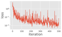
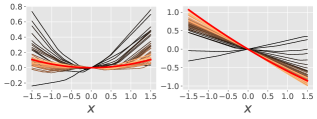
Refer to caption
(a) Evolution of loss estimate over first 500500500 optimization iterations.
Refer to caption
(b) Evolution of neural network N0(𝐱,𝐲)subscript𝑁0𝐱𝐲N_{0}(\mathbf{x},\mathbf{y}) (black to copper) approximating the initial value function v(𝐱,𝐲,0)𝑣𝐱𝐲0v(\mathbf{x},\mathbf{y},0) (red) over first 500500500 optimization iterations for a typical (left) and an extreme (right) observation y𝑦y.
Refer to caption
(c) Evolution of neural network N(𝐱,𝐲,t)𝑁𝐱𝐲𝑡-N(\mathbf{x},\mathbf{y},t) (black to copper) approximating the optimal control function 𝐜(𝐱,𝐲,t)subscript𝐜𝐱𝐲𝑡\mathbf{c}_{\star}(\mathbf{x},\mathbf{y},t) (red) over first 500500500 optimization iterations for a typical (upper row) and an extreme (lower row) observation y𝑦y.
Figure 6: Results for Ornstein–Uhlenbeck model with d=1𝑑1d=1 and σ𝐘=1.0subscript𝜎𝐘1.0\sigma_{\mathbf{Y}}=1.0 during initial training phase.
Refer to caption
(a) Evolution of loss estimate over 200020002000 optimization iterations under static and iterative CDT schemes.
Refer to caption
(b) Neural network approximation N0(𝐱,𝐲)subscript𝑁0𝐱𝐲N_{0}(\mathbf{x},\mathbf{y}) of the initial value function v(𝐱,𝐲,0)𝑣𝐱𝐲0v(\mathbf{x},\mathbf{y},0) after training with the static and iterative CDT schemes for a typical (left) and an extreme (right) observation y𝑦y.
Refer to caption
(c) Neural network approximation N(𝐱,𝐲,t)𝑁𝐱𝐲𝑡-N(\mathbf{x},\mathbf{y},t) of the optimal control function 𝐜(𝐱,𝐲,t)subscript𝐜𝐱𝐲𝑡\mathbf{c}_{\star}(\mathbf{x},\mathbf{y},t) after training with the static and iterative CDT schemes for a typical (upper row) and an extreme (lower row) observation y𝑦y.
Figure 7: Results for Ornstein–Uhlenbeck model with d=1𝑑1d=1 and σ𝐘=1.0subscript𝜎𝐘1.0\sigma_{\mathbf{Y}}=1.0 after training.
Refer to caption
(a) Evolution of loss estimate over first 500500500 optimization iterations.
Refer to caption
(b) Evolution of neural network N0(𝐱,𝐲)subscript𝑁0𝐱𝐲N_{0}(\mathbf{x},\mathbf{y}) (black to copper) approximating the initial value function v(𝐱,𝐲,0)𝑣𝐱𝐲0v(\mathbf{x},\mathbf{y},0) over first 500500500 optimization iterations for a typical (left) and an extreme (right) observation y𝑦y.
Refer to caption
(c) Evolution of neural network N(𝐱,𝐲,t)𝑁𝐱𝐲𝑡-N(\mathbf{x},\mathbf{y},t) (black to copper) approximating the optimal control function 𝐜(𝐱,𝐲,t)subscript𝐜𝐱𝐲𝑡\mathbf{c}_{\star}(\mathbf{x},\mathbf{y},t) over first 500500500 optimization iterations for a typical (upper row) and an extreme (lower row) observation y𝑦y.
Figure 8: Results for logistic diffusion model with θ4=1.069subscript𝜃41.069\theta_{4}=1.069 during initial training phase.
Refer to caption
(a) Evolution of loss estimate over 200020002000 optimization iterations under static and iterative CDT schemes and various levels of informative observations.
Refer to caption
(b) Neural network approximation N0(𝐱,𝐲)subscript𝑁0𝐱𝐲N_{0}(\mathbf{x},\mathbf{y}) of the initial value function v(𝐱,𝐲,0)𝑣𝐱𝐲0v(\mathbf{x},\mathbf{y},0) after training with the static and iterative CDT schemes for a typical (left) and an extreme (right) observation y𝑦y.
Refer to caption
(c) Neural network approximation N(𝐱,𝐲,t)𝑁𝐱𝐲𝑡-N(\mathbf{x},\mathbf{y},t) of the optimal control function 𝐜(𝐱,𝐲,t)subscript𝐜𝐱𝐲𝑡\mathbf{c}_{\star}(\mathbf{x},\mathbf{y},t) after training with the static and iterative CDT schemes for a typical (upper row) and an extreme (lower row) observation y𝑦y.
Figure 9: Results for logistic diffusion model with θ4=1.069subscript𝜃41.069\theta_{4}=1.069 after training.
Refer to caption
(a) Evolution of loss estimate over 200020002000 optimization iterations under static and iterative CDT schemes and various levels of informative observations.
Refer to caption
(b) Neural network approximation N0(𝐱,𝐲)subscript𝑁0𝐱𝐲N_{0}(\mathbf{x},\mathbf{y}) of the initial value function v(𝐱,𝐲,0)𝑣𝐱𝐲0v(\mathbf{x},\mathbf{y},0) after training with the static (left column) and iterative (right column) CDT schemes for a typical (upper row) and an extreme (lower row) observation y𝑦y.
Refer to caption
Refer to caption
(c) Neural network approximation N(𝐱,𝐲,t)𝑁𝐱𝐲𝑡-N(\mathbf{x},\mathbf{y},t) of the optimal control function 𝐜(𝐱,𝐲,t)subscript𝐜𝐱𝐲𝑡\mathbf{c}_{\star}(\mathbf{x},\mathbf{y},t) after training with the static (upper row) and iterative (lower row) CDT schemes for a typical and (columns 1-3) an extreme (columns 4-6) observation y𝑦y.
Figure 10: Results for cell model with σ𝐘=0.5subscript𝜎𝐘0.5\sigma_{\mathbf{Y}}=0.5 after training.