A Compressed Sensing Faraday Depth Reconstruction Framework for the MeerKAT MIGHTEE-POL Survey.

Abstract

In this work we present a novel compute framework for reconstructing Faraday depth signals from noisy and incomplete spectro-polarimetric radio datasets. This framework is based on a compressed-sensing approach that addresses a number of outstanding issues in Faraday depth reconstruction in a systematic and scaleable manner. We apply this framework to early-release data from the MeerKAT MIGHTEE polarisation survey.

1 Introduction

The MeerKAT MIGHTEE survey is imaging four extragalactic fields, COSMOS, XMM-LSS, CDFS, and ELAIS S1 [1]. All fields are being observed at L-band from 880–1680 MHz, in multiple pointings that will be mosaiced to a final image with a broad-band sensitivity of $\sim$2 $\mu$Jy beam^-1 [2]. The MIGHTEE project is creating science data products for total intensity, broad-band continuum science, HI spectra-line science, and spectro-polarimetric science. Initial data sets for shared-risk early science projects are being produced in each category from early observations of COSMOS and XMMLSS.

Next-Generation radio telescopes such as the Square Kilometre Array (SKA) will produce raw data volumes orders of magnitude larger than those from current facilities. Already the data volumes from existing SKA precursors such as MeerKAT are revealing big data and high-throughput computing (HTC) challenges. An example of this is the study of cosmic magnetism using Faraday Rotation information. In this scenario, multiple lines of sight from a linearly polarized spectral image cube must be passed through a non-linear optimization algorithm in order to obtain a 3D Faraday depth reconstruction. Addressing this problem not only involves the application of parallelism and HTC techniques, but also the introduction of software paradigms that facilitate automated workflows and pipeline operations.

This paper describes the application of a novel Faraday compute framework for compressed sensing (CS) reconstruction of spectro-polarimetric data from the MIGHTEE polarisation (MIGHTEE-POL) science case.

2 CS for Faraday depth reconstruction

Compressed sensing (CS) is a novel paradigm that contradicts the Nyquist-Shannon theorem for data acquisition under certain circumstances. The degree of success of this method depends on the amount of information that can be supplied to constrain the signal solution while being consistent with the measurements [3]. These constraints are sparsity, non-negativity, compactness, and the smoothness of the signal. To fully recover a signal, $x$, a compressible representation as a $k$-sparse vector must be imposed. Mathematically, a signal is defined to be sparse or compressible if it contains a small number, $k$, of non-zero or significant values. Typically, signals are not themselves sparse, but they can have a sparse representation in some basis $\Phi$. In this case we can refer to $x$ being $k$-sparse considering $x=\Phi c$, where $\left\lVert c\right\rVert_{0}\leq k$. The main problem with this approach is that the zero-norm function, which counts the non-zero elements of a vector, is non-convex and finding a solution that approximates the true minimum is generally a non-deterministic polynomial-time hard (NP-hard) problem and computationally very intensive [4].

However, [5] and [6] discovered that under general conditions it is possible to solve (relax) the above problem by using basis pursuit or enforcing convexity in the $\left\lVert\cdot\right\rVert_{0}$. That is, considering a Laplacian prior or a L1 regularization as

$$\hat{x}=\operatorname*{arg\,min}_{x}\left\lVert x\right\rVert_{1}\;\text{subject to}\;x\in\mathcal{B}(y),$$ (1)

and that $\mathcal{B}(y)$ is convex, then the problem has become computationally feasible and can be solved with efficient methods from convex optimization. Here, the $L_{1}$ norm of a vector is defined as the sum of the absolute values of each component of the vector.

In the presence of noise, Equation 1 can also be written as an unconstrained problem:

$$\hat{x}=\operatorname*{arg\,min}_{x}\frac{1}{2}\left\lVert Ax-y\right\rVert_{2}^{2}+\eta\left\lVert x\right\rVert_{1}\;,$$ (2)

where the first term is equivalent to the squared sum of the data residuals and $\eta$ is a regularization parameter that determines the relative importance between minimizing the $L_{1}$-norm and the measurement residuals.

For reconstruction of Faraday depth signals, one of the first works in this area was [7], which demonstrated the applicability of the known Mexican Hat wavelet to decompose the Faraday depth Spectrum. Later [8] reconstructed synthetic data from [9] and used three algorithms for the reconstruction of different kinds of structure. The difference between the algorithms lies in which space these structures are sparse. Another work that reconstructs Faraday depth spectrum signals using CS was [10]. This work uses the Matching-Pursuit (MP) algorithm, an L1-norm regularization and a boxcar dictionary in order to reconstruct both thin and thick Faraday signals. The work of [11] used a trade-off between sparsity and smoothness in Faraday depth space using regularizations such as the $L_{1}$-norm and Total Variation (TV) or Total Squared Variation (TSV). This used a Faraday depth model from [12] with both Faraday thin and thick structures in a frequency band from $300$ to $3000$ MHz to test the procedure. The results were compared with an RMCLEAN version from [13]. The work made by [14] improved on this last using an iterative restoration algorithm based on the projected gradient descent where at each iteration, different assumptions of the Faraday depth spectrum can be made such as sparsity and considering that some parts of the spectrum are the result of the Rotation Measure spread function (RMSF). In this work the smoothness of the polarization angle can also be added as a constraint.

There are two things to note across these two most recent works. Both create data in Faraday depth space and then transform into $\lambda^{2}$-space using a DFT. However, doing this implies that the $\lambda^{2}$-space is implicitly regularly-spaced. It is worth noting that an irregular $\lambda^{2}$-space not only adds an additional layer of noise to the problem but also a problem similar to that seen in image synthesis. Secondly the simulations in these works do not account for frequency channel excision due to RFI, instrumental problems or calibration.

3 The cs-romer framework

In this work we propose a CS-framework that solves the problem statement in Equation 2, extending the objective function to impose edge-smoothed constraints when needed, such that

$$\hat{x}=\operatorname*{arg\,min}_{x}\Biggl{\{}f(x)+g(x)\Biggr{\}},$$ (3)

where $f(x)$ is commonly seen in the literature as the data or $\chi^{2}$ term, which is a function of the observed polarized intensity measurements as a function of $\lambda^{2}$, the model measurements or signal estimate, and the variance for each channel. $\chi^{2}$ is considered a convex smooth function and $g(x)$ is a convex function that is non-differentiable in some region such that

$$g(x)=\eta_{1}\text{L1}(x)+\eta_{2}{\rm TV^{\ast}}(x)\;,$$

where $x$ can be the signal itself or a wavelet representation and TV^∗ is either the TV or TSV norm.

First, the framework calculates $\lambda^{2}_{\text{min}}$ and $\lambda^{2}_{\text{max}}$. Then, $\Delta\lambda^{2}$ and $\delta\lambda^{2}$ are computed, defining the maximum observable Faraday depth, the resolution in Faraday depth space and the largest scale in Faraday space to which the data are inherently sensitive. The framework selects the cell-size in Faraday depth space as $\phi_{R}=\delta\phi/\rho$, where $\rho$ is the oversampling factor which can be selected as $4$ or $5$. We can use $||\phi_{\text{max}}||$ to calculate the length of the grid in Faraday depth space. Since our observed measurements belong to an irregular space and Faraday depth space is on a regular grid the framework offers two options to estimate the model data. The most intuitive option is perhaps to grid the observed measurements, in which case the framework uses a DFT or FFT. The second option is to use the Non-Uniform Fast Fourier Transform (NUFFT), which performs an FFT on non-uniform sampled data using an FFT on the signal and then a min-max interpolation.

Having decided on a method with which to approximate the model data points, the next step is to use an optimization method to minimize the objective function (see Equation 3). In this work we have chosen the Fast Iterative Shrinkage-Thresholding Algorithm (FISTA) [15]. This method is an enhancement of the ISTA method and has been used before in Faraday spectra reconstruction [8].

Many attempts have been made to automatically calculate the regularization parameters, $\eta_{1}$ and $\eta_{2}$, e.g. [16, 17, 18, 19]. For this framework, and only for L1 regularization, we adopt the error bound calculation in [20, 21]. Additionally, we have adopted the adaptive regularization method from [8] where on each iteration $1\sigma$ is subtracted from $\eta_{1}$.

In the case where the signal can be represented by a wavelet dictionary, our framework offers the set of discrete wavelet transforms (DWT) from the package pywt [22]. However, sometimes the DWT can cause problems due to its shift variance and poor directional properties [23]. As an alternative, and as a way to reconstruct both thin and thick Faraday structures, we have added the Undecimated Wavelet Transform (UWT) 1D functions from [22] to our framework.

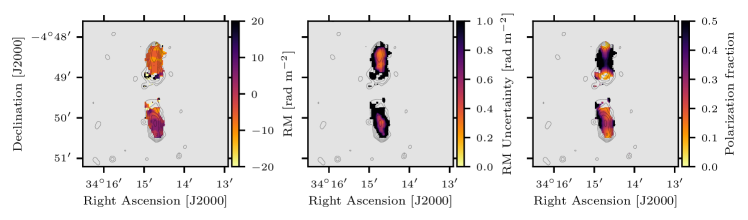
Figure 1: XMM-LSS Radio galaxy RM. From left to right: the rotation measure, the rotation measure uncertainty at the peak and the polarization fraction. The contours show the total intensity image at 5 $\sigma$ with increments of 2 $\sigma$.

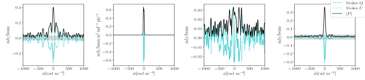
Figure 2: Single LOS from the radio galaxy in Figure 1, see text for details. From left to right: the dirty, the model, the residual and the restored Faraday spectra; $\pm$5 $\sigma_{\phi}$ limits are shown as a shaded area.

4 Wavelet and performance evaluation

Depending on the data, Faraday depth signals might have different structures. i.e thin sources, thick sources or both. To select the wavelet which best represents the signal, we simulate data given a known radio-telescope configuration with cs-romer. We use these data to create multiple realisations of data flagging and noise levels, which are then reconstructed using the full set of wavelet families. From these we select the best wavelet by evaluating the peak signal-to-noise ratio (PSNR), root mean squared error (RMSE), the Akaike’s Information Criterion (AIC) and Bayesian Information Criterion (BIC). In other words, we select the wavelet which results in the reconstruction with highest PSNR, lowest RMSE and lowest AIC and BIC.

5 Application to MIGHTEE-POL data

MIGHTEE-POL QU floating-point data cubes have dimensions of 6144$\times$6144$\times$239$\times$2, making them nearly 67.22 GB in size. Moreover, the regular-spaced Faraday Depth cubes are 6144$\times$6144$\times$373$\times$2 for XMM-LSS, which results in a data volume of 104.9 GB. Therefore the reconstruction of one field from the MIGHTEE-POL survey data requires $\sim$160 GB of memory. Even though this can be seen as a big data problem, each line of sight (LOS) can be processed independently and therefore, a big computing problem arises since it is not optimal to run 6144$\times$6144 optimizations sequentially. Thus, to speed up the reconstruction we use the joblib python library. Moreover, we only make calculations on those lines of sight where total intensity is over 3$\sigma_{I}$ and polarization intensity over 3$\sigma_{P}$. This decreases the total number of LOS by 99.75% for the XMM-LSS field. Here we use a canonical spectral index value of 0.7 for all LOS, but more generally the cs-romer framework can accept a casa spectral index map. The Faraday depth parameters for the XMM-LSS field are $\delta\phi=41.6$, max-scale$=97.3$ and $||\phi_{\text{max}}||=2057.7$, all in units of rad m^-2. The reconstruction takes 81.7 minutes on a server with 2 Intel(R) Xeon(R) Gold 5222 3.80 GHz CPUs and 1.5 TB RAM. Figure 1 shows the reconstructed RM, the RM uncertainty and the polarization for a radio galaxy selected from the XMM-LSS survey field. Additionally, Figure 2 shows the dirty, model, residual and restored Faraday spectra for the LOS with highest Stokes I intensity from this radio galaxy.

6 Conclusions

In this work we have presented the cs-romer compute framework, a CS approach to reconstructing Faraday depth spectra from noisy and incomplete spectro-polarimetric radio measurements. We have demonstrated that cs-romer can be used in a big-data and HTC scenario such as that appropriate for MIGHTEE-POL. In future work, we intend to decrease the reconstruction time further by distributing the framework across multiple compute nodes and exploring the impact of big data libraries such as dask.

7 Acknowledgements

MC acknowledges support from ANID PFCHA/DOCTORADO BECAS CHILE/2018-72190574. AMS and MB gratefully acknowledge support from the UK Alan Turing Institute under grant reference EP/V030302/1. MB gratefully acknowledges support from the UK Science & Technology Facilities Council (STFC).

References

- [1] M. Jarvis and R. Taylor et al., “The MeerKAT International GHz Tiered Extragalactic Exploration (MIGHTEE) Survey,” Proceedings of Science, vol. MeerKAT Science: On the Pathway to the SKA, Stellenbosch, 25-27 May 2016, p. 6, 2016.
- [2] I. Heywood and M. Jarvis et al., “MIGHTEE: total intensity radio continuum imaging and the COSMOS / XMM-LSS Early Science fields,” Monthly Notices of the Royal Astronomical Society, vol. 509, p. 2150–2168, 2021.
- [3] G. A. Richard Thompson, James M. Moran, Interferometry and Synthesis in Radio Astronomy. Weinheim: WILEY-VCH Verlag GmbH & Co. KGaA, 2004.
- [4] B. Natarajan, “Sparse approximate solutions to linear systems,” SIAM Journal on Computing, vol. 24, no. 2, pp. 227–234, 1995.
- [5] D. L. Donoho, “Compressed sensing,” IEEE Trans. Inf. Theor., vol. 52, no. 4, pp. 1289–1306, Apr. 2006.
- [6] E. J. Candes and T. Tao, “Near-optimal signal recovery from random projections: Universal encoding strategies?” IEEE Transactions on Information Theory, vol. 52, no. 12, pp. 5406–5425, Dec 2006.
- [7] P. Frick, D. Sokoloff, R. Stepanov, and R. Beck, “Wavelet-based Faraday rotation measure synthesis,” Monthly Notices of the Royal Astronomical Society: Letters, vol. 401, no. 1, pp. L24–L28, 01 2010.
- [8] F. Li, S. Brown, T. J. Cornwell, and F. de Hoog, “The application of compressive sampling to radio astronomy - ii. faraday rotation measure synthesis,” A&A, vol. 531, p. A126, 2011.
- [9] M. A. Brentjens and A. G. de Bruyn, “Faraday rotation measure synthesis,” A&A, vol. 441, no. 3, pp. 1217–1228, 2005.
- [10] M. Andrecut, J. M. Stil, and A. R. Taylor, “Sparse faraday rotation measure synthesis,” The Astronomical Journal, vol. 143, no. 2, p. 33, dec 2011.
- [11] K. Akiyama, T. Akahori, Y. Miyashita, S. Ideguchi, R. Yamaguchi, S. Ikeda, and K. Takahashi, “Faraday tomography with sparse modeling,” 2018.
- [12] S. Ideguchi, Y. Tashiro, T. Akahori, K. Takahashi, and D. Ryu, “Faraday dispersion functions of galaxies,” The Astrophysical Journal, vol. 792, p. 51, 2014.
- [13] Y. Miyashita, S. Ideguchi, and K. Takahashi, “Performance test of RM CLEAN and its evaluation with chi-square value,” Publications of the Astronomical Society of Japan, vol. 68, no. 3, 04 2016, 44.
- [14] S. Cooray, T. T. Takeuchi, T. Akahori, Y. Miyashita, S. Ideguchi, K. Takahashi, and K. Ichiki, “An iterative reconstruction algorithm for faraday tomography,” Monthly Notices of the Royal Astronomical Society, vol. 500, no. 4, p. 5129–5141, Nov 2020.
- [15] A. Beck and M. Teboulle, “A fast iterative shrinkage-thresholding algorithm for linear inverse problems,” SIAM Journal on Imaging Sciences, vol. 2, no. 1, pp. 183–202, 2009.
- [16] W. Karl, “3.6 - regularization in image restoration and reconstruction,” in Handbook of Image and Video Processing (Second Edition), A. BOVIK, Ed. Burlington: Academic Press, 2005, pp. 183–V.
- [17] P. C. Hansen, “The l-curve and its use in the numerical treatment of inverse problems,” in in Computational Inverse Problems in Electrocardiology, ed. P. Johnston, Advances in Computational Bioengineering. WIT Press, 2000, pp. 119–142.
- [18] M. Belge, M. E. Kilmer, and E. L. Miller, “Efficient determination of multiple regularization parameters in a generalized l-curve framework,” Inverse Problems, vol. 18, no. 4, pp. 1161–1183, jul 2002.
- [19] Y. Shi, S. Y. Low, and K. F. Cedric Yiu, “Hyper-parameterization of sparse reconstruction for speech enhancement,” Applied Acoustics, vol. 138, pp. 72–79, 2018.
- [20] R. E. Carrillo, J. D. McEwen, and Y. Wiaux, “PURIFY: a new approach to radio-interferometric imaging,” Monthly Notices of the Royal Astronomical Society, vol. 439, pp. 3591–3604, Apr. 2014.
- [21] L. Pratley, J. D. McEwen, M. d’Avezac, R. E. Carrillo, A. Onose, and Y. Wiaux, “Robust sparse image reconstruction of radio interferometric observations with purify,” Monthly Notices of the Royal Astronomical Society, vol. 473, pp. 1038–1058, 2017.
- [22] G. R. Lee, R. Gommers, F. Waselewski, K. Wohlfahrt, and A. O’Leary, “Pywavelets: A python package for wavelet analysis,” Journal of Open Source Software, vol. 4, no. 36, p. 1237, 2019.
- [23] N. A. Golilarz and H. Demirel, “Image de-noising using un-decimated wavelet transform (uwt) with soft thresholding technique,” in 2017 9th International Conference on Computational Intelligence and Communication Networks (CICN), 2017, pp. 16–19.