Flexible Group Fairness Metrics for Survival Analysis

Abstract.

Algorithmic fairness is an increasingly important field concerned with detecting and mitigating biases in machine learning models. There has been a wealth of literature for algorithmic fairness in regression and classification however there has been little exploration of the field for survival analysis. Survival analysis is the prediction task in which one attempts to predict the probability of an event occurring over time. Survival predictions are particularly important in sensitive settings such as when utilising machine learning for diagnosis and prognosis of patients. In this paper we explore how to utilise existing survival metrics to measure bias with group fairness metrics. We explore this in an empirical experiment with 29 survival datasets and 8 measures. We find that measures of discrimination are able to capture bias well whereas there is less clarity with measures of calibration and scoring rules. We suggest further areas for research including prediction-based fairness metrics for distribution predictions.

1. Introduction

The use of machine learning (ML) models, especially in the context of clinical decision making (Topol, 2019) can lead to, or exacerbate, disparities in health outcomes for marginalized populations (Nordling, 2019; Obermeyer et al., 2019; Vollmer et al., 2020). This can arise due to multiple reasons, such as access to different standards of care (Bailey et al., 2017), historical inequity (Chen et al., 2020; Hall et al., 2015) or under-representation in data collection (Buolamwini and Gebru, 2018; Larrazabal et al., 2020). This can lead to models with differing (predictive) effectiveness depending on the subpopulation or models that perpetuate historical injustices if they are subsequently used to inform medical decisions (Veinot et al., 2018). The goal of algorithmic fairness is to detect and mitigate such biases (Mehrabi et al., 2021; Barocas et al., 2019). This has been discussed in great detail in classification and regression settings (Rajkomar et al., 2018; Mehrabi et al., 2021; Pfohl et al., 2021), however very little discussion exists for survival analysis. This is problematic given the sensitive nature of survival predictions. For example, hospitals with insufficient resources may require survival models to accurately and fairly rank patient outcome risks (Ryan et al., 2020; Liang et al., 2020; Sprung et al., 2020). It is crucial that algorithmic fairness is considered in the survival setting. Zhang and Weiss (Zhang and Weiss, 2022) have begun exploring debiasing methods for survival analysis, however only a limited number of measures are considered. In this article we examine whether existing metrics that are used in survival analysis can be adapted to detect unfairness in survival models. The code required to reproduce the results in this paper is publicly available at https://github.com/Vollmer-Lab/survival_fairness. For a comprehensive overview to fairness and survival analysis we recommend Mitchell et al. (2021) (Mitchell et al., 2021) and Wang et al. (2019) (Wang et al., 2019) respectively.

2. Related Work

2.1. Fairness metrics

Many notions of fairness exist, including individual fairness (Dwork et al., 2012), causal/counterfactual fairness (Kusner et al., 2017; Zhang and Bareinboim, 2018; Chiappa, 2019), group fairness, and intersectional fairness. Individual fairness measures require defining a metric space that encodes differences between individuals (Dwork et al., 2012) and it is unclear in general how such a metric should be chosen. Causal fairness measures require defining causal relationships between covariates and protected attributes and outcomes, for example in the form of a directed acyclic graph (Kusner et al., 2017), which is especially challenging to construct in high dimensional settings. In this paper we focus on group fairness definitions. These metrics have the advantage that they can be measured without causal assumptions and without defining a metric over individuals.

Discrimination criteria can be understood as measuring adherence to one of the following independence statements defined based on a model’s predicted score or class, $R$, protected attribute, $S$, and target variable, $Y$: Independence: $R\perp S$, Separation: $R\perp S\mid Y$ and Sufficiency $Y\perp S\mid R$, (Barocas and Selbst, 2016). We will refer to metrics that require one of these three independence statements above as (statistical) group fairness metrics since independence is observed at the level of the protected groups. Group fairness metrics are usually defined for the classification setting, however many of them naturally lend themselves to regression scenarios or can be adapted simply (Steinberg et al., 2020). Intersectional fairness (Buolamwini and Gebru, 2018) extends group fairness for a more fine-grained, and intersectional, assessment of bias. For example, group fairness measures may assess if a dataset is unbiased across race and gender, whereas an intersectional fairness measures will also assess if the interaction between race and gender are also unbiased.

2.2. Fairness metrics in survival analysis

Applications of fairness metrics in clinical decision making have been studied by Pfohl et al. (Pfohl et al., 2021), however this is restricted to the classification setting. Whilst classification metrics may be directly extended to the regression setting, the same does not hold for the more complex survival setting. This is due to: 1) time-to-event datasets including censoring, i.e. patients who are not observed to experience the event of interest; and 2) the prediction of interest is a distribution and not a single value.

We could find only two strategies evaluating survival fairness in the literature. The first is a transformation of the survival objective, the second is metric based; we briefly discuss each in turn. One approach to evaluating fairness in a survival setting is to assess fairness for binary survival predictions at fixed time points (Barda et al., 2020), e.g. three years in the future. This strategy can yield viable and fair predictors if the selected horizon perfectly coincides with the time-point at which decisions are made. However, this is generally not the case and therefore evaluation of such models usually results in over-confidence in model performance due to ‘improper’ evaluation (Blanche et al., 2019), thus this strategy is not fair. On the other hand, Keya et al (Keya et al., 2021) proposed predictive metrics – individual, group, and intersectional – for survival fairness that do not require any objective transformation. Whilst this is a great step forward, their metrics are only applicable to linear predictors, such as from the Cox Proportional Hazards (PH) model (Cox, 1972). Whilst the Cox PH is arguably the most popular model in survival analysis, this limitation means that their metrics cannot be applied to the majority of machine learning models.

3. Fairness in survival analysis

Survival analysis is a task in which one attempts to predict the probability of an event occurring over time. For example, predicting the risk of a patient dying of a disease after diagnosis, predicting when a customer will default on a loan (‘duration analysis’), or predicting the probability of a lightbulb failing over time (‘reliability analysis’). Survival analysis is distinct from regression as we are interested in making predictions from censored time-to-event data. A censored observation is one in which the event of interest does not occur. Survival models are fit to estimate the functional relationship between a set of covariates $X$ and time until an event of interest takes place $Y$. We assume, for all observations, that there exists both a hypothetical survival time $Y$ and censoring time $C$ (the last recorded time for an observation). We define $T:=\text{min}(Y,C)$ as the observed outcome time and $\Delta:=\mathbb{I}(Y=T)$ as the survival indicator. Survival models are fit on the survival tuple $(X,T,\Delta)$. For this paper we only consider the right-censoring survival setting. Data is assumed to consist of $n$ observations drawn i.i.d. from a data-generating distribution $\mathrm{P_{x,y}}$. In fairness contexts we further assume there exists one or multiple sensitive attributes, $S$, assigning groups to each observation.

3.1. Experiment

Analysis

We are interested in understanding how well existing losses capture bias in survival datasets. We apply biasing algorithms to 29 published survival datasets (Appendix D), fit a random survival forest (RSF) (Ishwaran et al., 2008) on these biased datasets and then evaluate fairness as $F_{L}=|L_{A}-L_{D}|$ where $F_{L}$ is the fairness measured by loss $L$, and $L_{A},L_{D}$ are the model performance on the advantaged and disadvantaged subgroups respectively measured by loss $L$. Analysis is performed with mlr3proba (Sonabend et al., 2021b) in R (R Core Team, 2017). We fit an RSF as it robustly returns multiple prediction types (Sonabend et al., 2021a) that can be assessed with calibration, discrimination and scoring rule measures. We increased the proportion, $\sigma$, of biased observations in the disadvantaged data from 0% to 90% and asserted that a loss, $L$, could capture bias in our datasets if there was a significant Spearman rank correlation between $F_{L}$ and $\sigma$, and a significant t-test after regressing $F_{L}$ on $\sigma$.

Biasing algorithms

We created biasing methods that mimic identified real-world sources of bias (Mehrabi et al., 2019). Our first method simulates measurement bias by randomly permuting the covariates for an increasing proportion of disadvantaged observations for each dataset, whereas our second method simulates representation bias by increasingly undersampling disadvantaged groups for each dataset. These are fully described in Appendix A.

Measures

We consider a range of calibration, discrimination, and scoring rule measures common in the survival literature. We avoid evaluation bias (Mehrabi et al., 2019) by only including (strictly) proper scoring rules as other (improper) scoring rules may not accurately identify a superior model over an inferior one. We consider the right-censored log-likelihood (RCLL) (Avati et al., 2018), reweighted survival Brier score (RSBS) (Graf et al., 1999; Sonabend, 2021), reweighted integrated survival logloss (RISL) (Graf et al., 1999; Sonabend, 2021), survival negative log-likelihood (SNL) (Sonabend, 2021), van Houwelingen’s alpha (CalA) (Van Houwelingen, 2000), D-calibration (CalD) (Haider et al., 2020), Harrell’s C ($C_{H}$) (Harrell et al., 1982, 1984), and Uno’s C ($C_{U}$) (Uno et al., 2011). Scoring rules are standardised against a Kaplan-Meier baseline (Graf and Schumacher, 1995; Kaplan and Meier, 1958).

Results

We now assess how well the metrics recover increased unfairness, controlled by $\sigma$. Regressing $F_{L}$ on $\sigma$, we find that for the permutation biasing method, $\sigma$ was a significant predictor of $F_{L}$ for RSBS, RISL, $C_{H}$, $C_{U}$, $CalA$. We also find that for RCLL there is a significant correlation between $F_{L}$ and $\sigma$ however the regression slope is too small to be meaningful. There is also a significant relationship between $F_{L}$ and $\sigma$ for SNL after applying the undersampling algorithm (Table 1 and Appendix C).

Table 1. Let $F_{L}=\alpha+\sigma\beta$ be our regression model. Table shows intercept, $\alpha$, slope, $\beta$, and Spearman rank correlation ($\rho$) for each of the measures and permutation (left) and undersampling (right) biasing methods. An ‘*’ indicates a p-value less than 0.05 after Holm’s correction.

Measure	$\alpha$	$\beta$	$\rho$	$\alpha$	$\beta$	$\rho$
	Permutation			Undersampling
RSBS	0.049	0.078∗	0.976∗	0.035	0.066∗	0.855∗
RISL	0.045	0.063∗	0.976∗	0.033	0.058∗	0.891∗
SNL	0.018	0.001	0.248	0.014	0.083∗	1.000∗
RCLL	0.018	0.009	0.879∗	0.022	0.088∗	1.000∗
$C_{H}$	0.024	0.129∗	1.000∗	0.017	0.083∗	1.000∗
$C_{U}$	0.031	0.124∗	1.000∗	0.024	0.078∗	0.976∗
CalA	0.027	0.011∗	0.891∗	-0.015	0.197∗	0.952∗
CalD	2.686	0.487	0.721∗	2.861	0.646	0.612

3.2. Discussion

There is a significant relationship between $\sigma$ and $F_{L}$ for both measures of separation, $C_{H}$ and $C_{U}$. This is intuitive as the biasing methods prevent the model learning the true risk for disadvantaged observations and therefore cannot estimate the difference in risk between advantaged and disadvantaged observations. Secondly, $CalA$ does detect bias in the data whereas $CalD$ does not. $CalA$ evaluates if a model correctly predicts the number of events in the test set. In contrast, $CalD$ evaluates if the predicted survival functions are distributed according to $U(0,1)$. The significant result with $CalA$ indicates that the model cannot predict the number of events in the disadvantaged groups from either biasing method. Whereas the results with $CalD$ may indicate a more complex relationship between distributional calibration and fairness, which has already been demonstrated in the classification setting (Pleiss et al., 2017). Of the scoring rules, only RSBS and RISL could detect the bias from both methods with a regression slope of a meaningful magnitude. This is a promising finding as prior research has demonstrated the usefulness of scoring rules in evaluating fairness (Glymour and Herington, 2019).

4. Conclusions

Algorithmic fairness is an important concept to assess how much bias is present in datasets and subsequently picked up by models. This is especially important in survival analysis, which often overlaps with areas that requires strong ethical consideration. Despite this, the literature around survival fairness is in its infancy. In this paper we have performed a simple experiment to demonstrate how existing survival measures can be utilised to audit bias in algorithmic fairness. Measures of discrimination appear to be optimal for capturing bias however these do not paint a full picture as they ignore model calibration. We have found that the standardised scoring rules, RSBS and RISL, are interpretable, capture both calibration and discrimination, and can detect the bias from our algorithms. We believe future work should consider more complex biasing methods including temporal methods that introduce bias after a certain time-point. Finally, whilst predictive metrics have been proposed for risk predictions (Keya et al., 2021), these have yet to be reviewed in the literature and there is also potential to extend this work to survival distribution predictions. Our paper should help raise awareness that current methods of measuring fairness in survival are very limited and should stimulate interest and exploration in further development.

Disclaimer

This paper was prepared for informational purposes by the Artificial Intelligence Research group of JPMorgan Chase & Co. and its affiliates (“JP Morgan”), and is not a product of the Research Department of JP Morgan. JP Morgan makes no representation and warranty whatsoever and disclaims all liability, for the completeness, accuracy or reliability of the information contained herein. This document is not intended as investment research or investment advice, or a recommendation, offer or solicitation for the purchase or sale of any security, financial instrument, financial product or service, or to be used in any way for evaluating the merits of participating in any transaction, and shall not constitute a solicitation under any jurisdiction or to any person, if such solicitation under such jurisdiction or to such person would be unlawful.

Appendix A Biasing algorithm

We have a generic biasing algorithm (Algorithm 1) that is then specialised with two biasing methods. The algorithm splits the dataset into two equal-sized smaller datasets, one to add bias to ($D_{B}$) and one to leave untouched ($D_{U}$). Then we further split $D_{B}$ into two more datasets, $D_{BA},D_{BD}$, such that $\sigma\%$ of $D_{B}$ are in $D_{BD}$. The specific biasing algorithm, $G$, is then applied to $D_{BD}$. $D_{BA}$ and $D_{BD}$ are recombined and then three-fold cross-validation is utilised to evaluate model performance on $D_{B}$ and $D_{U}$ and fairness is computed. By splitting the data in this way we are able to: 1) ensure that the proportion of bias is simply controlled; 2) ensure that the model performance does not deteriorate for the unbiased dataset, i.e. if we do not split the original dataset in $D_{B}$ and $D_{U}$ then model performance will deteriorate overall due to the bias added to the disadvantaged group, whereas by splitting the dataset we are able to clearly distinguish between the ‘normal’ model performance (when no bias has been added), and the reduced performance due to the added bias.

Biasing method 1 - Permutation

For the first method we artifically add bias by randomly permuting the covariates of disadvantaged observations. This breaks the relationship between the covariates and outcomes and mimics the real-world problem of data being of lower-quality for disadvantaged groups of people.

Biasing method 2 - Undersampling

For the second method we artifically add bias by undersampling disadvantaged observations. In Algorithm 1 this amounts to deleting all observations in $D_{BD}$. This mimics the real-world problem of not capturing enough data for disadvantaged groups of people.

Algorithm 1 Input: $D=(X,T,\Delta)$, survival dataset. $\sigma$, proportion of disadvantaged observations to bias. $L$, survival loss. $M$, survival model. $G$, biasing algorithm. Output: $F_{L}$, fairness metric.

.

1:  for $i=1,...,10$ do

2:     $D_{B},D_{U}\leftarrow$ Randomly split $D$ into equal-sized datasets

3:     $D_{BA},D_{BD}\leftarrow$ Randomly split $D_{B}$ w.p. $\sigma$

4:     Apply $G$ to $D_{BD}$

5:     $D_{B}\leftarrow(D_{BA},D_{BD})$

6:     $L_{B}\leftarrow$ 3-fold CV of $D_{B}$ with model $M$ and loss $L$

7:     $L_{U}\leftarrow$ 3-fold CV of $D_{U}$ with model $M$ and loss $L$

8:     $F_{L;i}\leftarrow|L_{B}-L_{U}|$

9:  end for

10:  $F_{L}\leftarrow\sum_{i}F_{L;i}/10$

11:  return  $F_{L}$

Appendix B Metric definitions

Let $X,Y,C$ be random variables taking values in $\mathcal{X}\subseteq\mathbb{R}^{n},\mathcal{Y}\subseteq\mathbb{R},\mathcal{C}\subseteq\mathbb{R}$ respectively. In addition, define $T:=\min(Y,C)$, and $\Delta:=\mathbb{I}(Y=T)$. Finally let $(X_{i},Y_{i},C_{i},T_{i},\Delta_{i})\stackrel{{\scriptstyle\text{i.i.d.}}}{{\sim}}(X,Y,C,T,\Delta)$. We define the following measures and include a brief explanation of their interpretation and use.

• Reweighted survival Brier score (RSBS) (Graf et al., 1999; Sonabend, 2021)

  (1) $$L_{RSBS}(Y,T,\Delta|\hat{G}_{KM})=\frac{\Delta\int_{\mathcal{T}}(\mathbb{I}(T\leq\tau)-F_{Y}(\tau))^{2}\ d\tau}{\hat{G}_{KM}(T)}$$

  This is a strictly proper approximate survival loss that evaluates a survival distribution prediction by measuring the squared distance between the predicted survival probability and whether the event occurs. It is the CRPS with an inverse probability of censoring weighting (IPCW) adjustment.

• Reweighted integrated survival logloss (RISL) (Graf et al., 1999; Sonabend, 2021)

  (2) $$\begin{split}&L_{RISL}(Y,T,\Delta|\hat{G}_{KM})=\\ &\frac{\Delta\int_{\mathcal{T}}\mathbb{I}(T\leq\tau)\log[F_{Y}(\tau)]+\mathbb{I}(T>\tau)\log[S_{Y}(\tau)]\ d\tau}{\hat{G}_{KM}(T)}\end{split}$$

  This is a strictly proper approximate survival loss that evaluates a survival distribution prediction by measuring the logarithm of the predicted survival (or 1-survival) probability and whether the event occurs. It is the integrated loglikelihood with an inverse probability of censoring weighting (IPCW) adjustment

• Survival negative log-likelihood (SNL) (Sonabend, 2021)

  (3) $$L_{SNL}(Y,T,\Delta|\hat{G}_{KM})=-\frac{\Delta\log[f_{Y}(T)]}{\hat{G}_{KM}(T)}$$

  This is a strictly proper approximate survival loss that evaluates a survival distribution prediction by taking the logarithm of the predicted probability density function. It is essentially the ‘usual’ negative log-likelihood with an IPCW weighting.

• Right-censored log-likelihood (RCLL) (Avati et al., 2018)

  (4) $$L_{RCLL}(Y,T,\Delta)=-\log[\delta f_{Y}(T)+(1-\Delta)(S_{Y}(T))]$$

  This is a strictly proper survival loss that evaluates a survival distribution prediction by taking the logarithm of the predicted probability density function for ‘dead’ observations and the logarithm of the predicted survival function for censored observations.

• Harrell’s C ($C_{H}$) (Harrell et al., 1982, 1984)

  (5) $$\begin{split}C_{H}(\phi,T,\Delta)=\frac{\sum_{i\neq j}\mathbb{I}(T_{i}<T_{j},\phi_{i}>\phi_{j})\Delta_{i}}{\sum_{i\neq j}\mathbb{I}(T_{i}<T_{j})\Delta_{i}}\end{split}$$

  where $\phi$ are predicted risks.
  This is a concordance measure that evaluates the discrimination of a ranking prediction by asserting if predicted risks are concordant with observed survival times, i.e., if observation $i$ is predicted to be of higher risk of dying than observation $j$, then this prediction is concordant if $i$ dies before $j$.

• Uno’s C ($C_{U}$) (Uno et al., 2011)

  (6) $$\begin{split}&C_{U}(\phi,T,\Delta|\tau)=\\ &\frac{\sum_{i\neq j}W(T_{i})\mathbb{I}(T_{i}<T_{j},\phi_{i}>\phi_{j},T_{i}<\tau)\Delta_{i}}{\sum_{i\neq j}W(T_{i})\mathbb{I}(T_{i}<T_{j},T_{i}<\tau)\Delta_{i}}\end{split}$$

  where $\phi$ are predicted risks, $W(t_{i})=[\hat{G}_{KM}(t_{i})]^{-2}$, $\hat{G}_{KM}$ is the Kaplan-Meier estimator fit on $(T,1-\Delta)$, and $\tau$ is an upper-cutoff timepoint.
  This has the same interpretation as Harrell’s C but includes an IPCW adjustment to account for censoring.

• van Houwelingen’s alpha (CalA) (Van Houwelingen, 2000)

  (7) $$\alpha(\hat{H},T,\Delta)=\frac{\sum_{i}\Delta_{i}}{\sum_{i}\hat{H}_{i}(T_{i})}$$

  where $\hat{H}_{i}$ are individual predicted cumulative hazard functions.
  This is a calibration measures that evaluates if a predicted survival distribution is well-calibrated by asserting if the predicted expected number of events is equal (or close to equalling) the true number of observed events.

• D-calibration (CalD) – Algorithm in (Haider et al., 2020).
  This is a calibration measures that evaluates if a predicted survival distribution is well-calibrated by asserting if the predicted survival distributions are distributed Uniformly as expected.

Let $L_{M}$ be a scoring rule evaluated on a model $M$ and let $L_{K}$ be the same scoring rule evaluated on a prediction from the Kaplan-Meier baseline, then the explained residual variation (ERV) (Graf and Schumacher, 1995) of $L$ is defined as the percentage decrease of $L_{M}$ from $L_{K}$:

(8) $$\tilde{L}=1-\frac{L_{M}}{L_{K}}=\frac{L_{K}-L_{M}}{L_{K}}$$

This allows any scoring rule to be meaningfully interpreted as a percentage increase in performance over a baseline model. We standardise all the scoring rules above (RSVS, RISL, SNL, RCLL) with this method.

Appendix C Full results

The full results of running our experiment are provided below in tabular and graphical forms.

Table 2. Measures computed after running the permutation biasing algorithm a random survival forest, arithmetic mean taken over all datasets. $\sigma$ values are represented in the columns such that $\sigma=0$ means there is no bias in the disadvantaged dataset whereas $\sigma=0.9$ means 90% of observations are biased in the disadvantaged dataset. Measures with ‘(ERV)’ after them are standardised against a Kaplan-Meier baseline (Appendix B).

Measure / $\sigma$	0	0.1	0.2	0.3	0.4	0.5	0.6	0.7	0.8	0.9
	Permutation Biasing Method
$C_{H}$	0.034	0.036	0.046	0.054	0.073	0.089	0.102	0.118	0.131	0.138
$C_{U}$	0.038	0.043	0.054	0.06	0.076	0.096	0.109	0.12	0.132	0.141
CalA	0.028	0.027	0.03	0.029	0.03	0.034	0.036	0.036	0.036	0.036
CalD	2.679	2.676	2.647	2.961	2.832	3.062	3.154	3.014	3.027	3.005
RCLL	0.019	0.02	0.017	0.022	0.022	0.025	0.024	0.025	0.025	0.027
RISL	0.049	0.049	0.054	0.064	0.065	0.085	0.085	0.091	0.098	0.096
RSBS	0.054	0.054	0.061	0.072	0.075	0.098	0.096	0.105	0.116	0.113
SNL	0.017	0.018	0.017	0.02	0.017	0.019	0.017	0.019	0.018	0.019
	Undersampling Biasing Method
$C_{H}$	0.032	0.034	0.034	0.037	0.039	0.04	0.047	0.07	0.09	0.116
$C_{U}$	0.04	0.037	0.04	0.044	0.045	0.044	0.055	0.073	0.094	0.116
CalA	0.028	0.028	0.027	0.033	0.041	0.043	0.055	0.079	0.133	0.27
CalD	2.853	2.957	3.049	3.363	3.066	2.928	3.041	3.042	3.409	3.811
RCLL	0.026	0.03	0.039	0.045	0.055	0.063	0.075	0.086	0.093	0.101
RISL	0.042	0.049	0.046	0.043	0.051	0.048	0.055	0.07	0.085	0.104
RSBS	0.047	0.053	0.051	0.046	0.055	0.052	0.061	0.079	0.091	0.117
SNL	0.017	0.022	0.03	0.037	0.045	0.055	0.066	0.075	0.081	0.086

Figure 1. Boxplots of $\sigma$ against $F_{L}$ over the 29 datasets with the permutation biasing method applied. Blue lines are fit with local polynomial regression.

Eight boxplots with local polynomial regression smoothing showing the results of the regression of $\sigma$ against $F_{L}$ over the datasets biased with the permutation method. The boxplots show: $C_{H}$, $C_{U}$, $CalA$, $CalD$, $RCLL$, $RISL$, $RSBS$, $SNL$ with increasing slopes for $C_{H}$, $C_{U}$, $CalA$, $CalD$, $RISL$ and $RSBS$.

Figure 2. Spearman rank correlation of $\sigma$ against $F_{L}$ over the 29 datasets with the permutation biasing method applied. Pink bars indicate correlations with $p<0.05$ after correction by Holm’s method.

Eight vertical bars showing Spearman rank correlation of $\sigma$ against $F_{L}$ for $C_{H}$, $C_{U}$, $CalA$, $CalD$, $RCLL$, $RISL$, $RSBS$, $SNL$. All bars are pink except for $SNL$ indicating significant correlations.

Figure 3. Boxplots of $\sigma$ against $F_{L}$ over the 29 datasets with the undersampling biasing method applied. Blue lines are fit with local polynomial regression.

Eight boxplots with local polynomial regression smoothing showing the results of the regression of $\sigma$ against $F_{L}$ over the datasets biased with the undersampling method. The boxplots show: $C_{H}$, $C_{U}$, $CalA$, $CalD$, $RCLL$, $RISL$, $RSBS$, $SNL$ with increasing slopes for $C_{H}$, $C_{U}$, $CalA$, $RISL$ and $RSBS$.

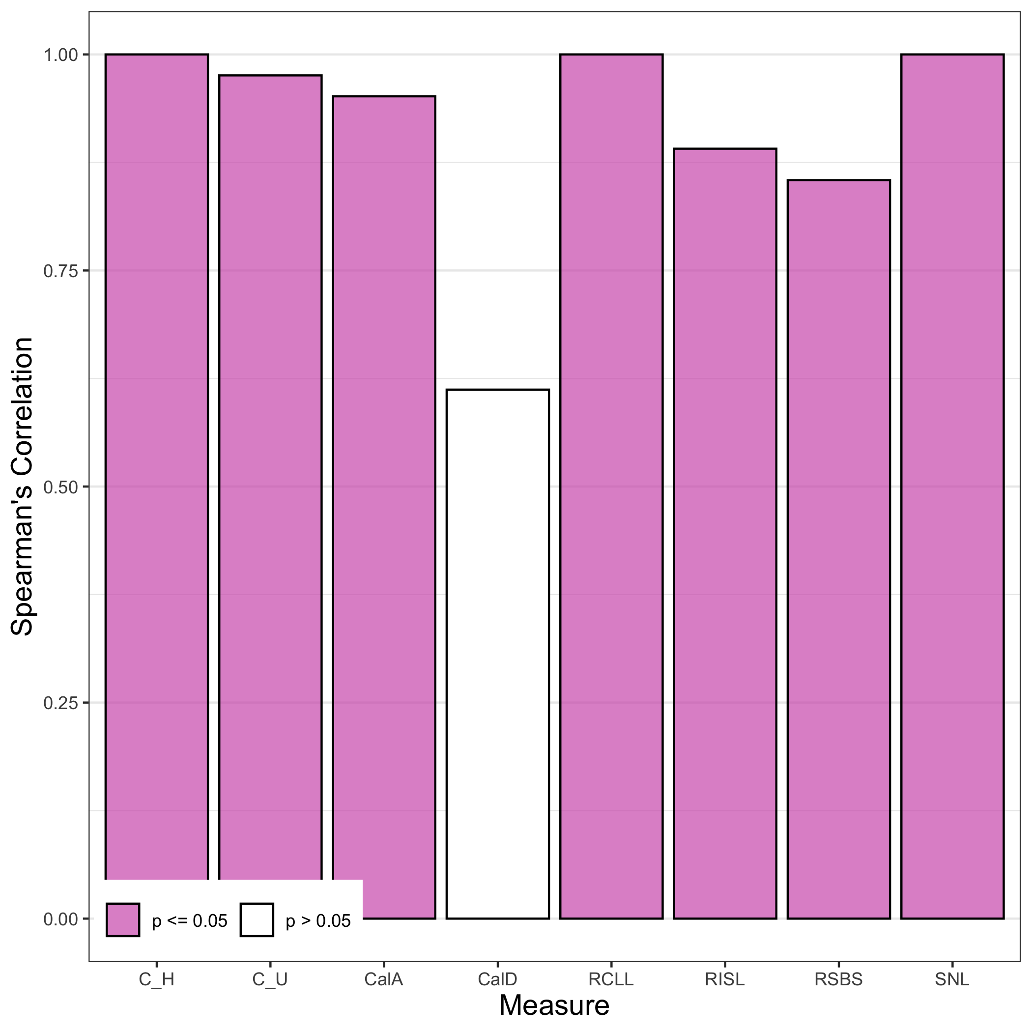
Figure 4. Spearman rank correlation of $\sigma$ against $F_{L}$ over the 29 datasets with the undersampling biasing method applied. Pink bars indicate correlations with $p<0.05$ after correction by Holm’s method.

Eight vertical bars showing Spearman rank correlation of $\sigma$ against $F_{L}$ for $C_{H}$, $C_{U}$, $CalA$, $CalD$, $RCLL$, $RISL$, $RSBS$, $SNL$. All bars are pink except for $CalD$ indicating significant correlations.

Appendix D Datasets

Table 3. Datasets used in experiments. 1. Dataset ID and citation. 2. Proportion of censoring in the dataset, rounded to nearest percentage point. 3-4. Number of continuous and discrete features respectively. 5-6. Total number of observations and features respectively. 7. Number of observed events in dataset. 8. R package in which the dataset is included.

Dataset1	Cens %2	$n_{C}^{3}$	$n_{D}^{4}$	n5	p6	$n_{E}^{7}$	Package8
aids.id (Carlin and Louis, 2018)	60	1	4	467	5	188	JM (Rizopoulos, 2010)
Aids2 (N. Venables and D. Ripley, 2002)	38	1	3	2814	4	1733	MASS (N. Venables and D. Ripley, 2002)
ALL (van Houwelingen and Putter, 2008)	63	0	4	2279	4	838	dynpred (Putter, 2015)
bladder0 (Sylvester et al., 2006)	48	0	3	397	3	206	frailtyHL (Putter, 2015)
CarpenterFdaData (Carpenter, 2002)	36	15	11	408	26	262	simPH
channing (Klein and Moeschberger, 2003)	62	1	1	458	2	176	KMsurv
child (Broström, 2021)	79	1	3	26574	4	5616	eha (Broström, 2021)
cost (Jørgensen et al., 1996)	22	3	10	518	13	404	pec (Mogensen et al., 2014)
e1684 (Kirkwood et al., 1996)	31	1	2	284	3	196	smcure (Cai et al., 2012)
flchain (Dispenzieri et al., 2012)	72	4	3	7871	7	1082	survival
FTR.data (Trébern-Launay et al., 2013)	86	0	2	2206	2	300	MRsurv (Foucher and Trebern-Launay, 2013)
gbsg (Katzman et al., 2018)	43	3	4	2232	7	1267	pycox (Kvamme, 2018)
grace (Hosmer Jr et al., 2011)	68	4	2	1000	6	324	mlr3proba (Sonabend et al., 2021c)
hdfail (Monaco et al., 2018)	94	1	4	52422	5	2885	frailtySurv (Monaco et al., 2018)
kidtran (Klein and Moeschberger, 2003)	84	1	3	863	4	140	KMsurv
liver (Andersen et al., 2012)	40	1	1	488	2	292	joineR (Williamson et al., 2008)
lung (Loprinzi et al., 1994)	28	5	3	167	8	120	survival
metabric (Katzman et al., 2018)	42	5	4	1903	9	1103	pycox
mgus (Kyle, 1993)	6	6	1	176	7	165	survival
nafld1 (Allen et al., 2018)	92	4	1	12588	5	322	survival
nwtco (Breslow and Chatterjee, 1999)	86	1	2	4028	3	571	survival
ova (Van Houwelingen et al., 1989)	26	1	4	358	5	266	dynpred
patient (Bender et al., 2018)	79	2	5	1985	7	416	pammtools (Bender and Scheipl, 2018)
rdata (M. Pohar and J. Stare, 2006)	47	1	3	1040	4	547	relsurv (M. Pohar and J. Stare, 2006)
reconstitution (Duchateau and Janssen, 2008)	19	0	2	200	2	162	parfm
std (Klein and Moeschberger, 2003)	60	3	18	877	21	347	KMsurv
STR.data (Trébern-Launay et al., 2013)	82	0	4	546	4	101	MRsurv
support (Katzman et al., 2018)	32	10	4	8873	14	2705	pycox
tumor (Bender and Scheipl, 2018)	52	1	6	776	7	375	pammtools
uis (Hosmer et al., 2008)	19	7	5	575	12	464	quantreg (Koenker, 2021)
veteran (Kalbfleisch and Prentice, 2011)	7	3	3	137	6	128	survival
wbc1 (The Benelux C M L Study Group, 1998)	43	2	0	190	4	109	dynpred
whas (Hosmer Jr et al., 2011)	48	3	6	481	9	249	mlr3proba

References

- (1)
- Allen et al. (2018) Alina M Allen, Terry M Therneau, Joseph J Larson, Alexandra Coward, Virend K Somers, and Patrick S Kamath. 2018. Nonalcoholic fatty liver disease incidence and impact on metabolic burden and death: A 20 year-community study. Hepatology (Baltimore, Md.) 67, 5 (may 2018), 1726–1736. https://doi.org/10.1002/hep.29546
- Andersen et al. (2012) Per K Andersen, Ornulf Borgan, Richard D Gill, and Niels Keiding. 2012. Statistical models based on counting processes. Springer Science & Business Media.
- Avati et al. (2018) Anand Avati, Tony Duan, Sharon Zhou, Kenneth Jung, Nigam H. Shah, and Andrew Ng. 2018. Countdown Regression: Sharp and Calibrated Survival Predictions. (jun 2018). arXiv:1806.08324 http://arxiv.org/abs/1806.08324
- Bailey et al. (2017) Zinzi D Bailey, Nancy Krieger, Madina Agénor, Jasmine Graves, Natalia Linos, and Mary T Bassett. 2017. Structural racism and health inequities in the USA: evidence and interventions. The Lancet 389, 10077 (2017), 1453–1463.
- Barda et al. (2020) Noam Barda, Dan Riesel, Amichay Akriv, Joseph Levy, Uriah Finkel, Gal Yona, Daniel Greenfeld, Shimon Sheiba, Jonathan Somer, Eitan Bachmat, et al. 2020. Developing a COVID-19 mortality risk prediction model when individual-level data are not available. Nature communications 11, 1 (2020), 1–9.
- Barocas et al. (2019) Solon Barocas, Moritz Hardt, and Arvind Narayanan. 2019. Fairness and Machine Learning. fairmlbook.org. http://www.fairmlbook.org.
- Barocas and Selbst (2016) Solon Barocas and Andrew Selbst. 2016. Big Data’s Disparate Impact. California Law Review 104, 1 (2016), 671–729. https://doi.org/10.15779/Z38BG31
- Bender and Scheipl (2018) Andreas Bender and Fabian Scheipl. 2018. pammtools: Piece-wise exponential Additive Mixed Modeling tools. arXiv:1806.01042 [stat] (2018). http://arxiv.org/abs/1806.01042
- Bender et al. (2018) Andreas Bender, Fabian Scheipl, Wolfgang Hartl, Andrew G Day, and Helmut Küchenhoff. 2018. Penalized estimation of complex, non-linear exposure-lag-response associations. Biostatistics 20, 2 (feb 2018), 315–331. https://doi.org/10.1093/biostatistics/kxy003
- Blanche et al. (2019) Paul Blanche, Michael W Kattan, and Thomas A Gerds. 2019. The c-index is not proper for the evaluation of -year predicted risks. Biostatistics 20, 2 (apr 2019), 347–357. https://doi.org/10.1093/biostatistics/kxy006
- Breslow and Chatterjee (1999) N E Breslow and N Chatterjee. 1999. Design and analysis of two-phase studies with binary outcome applied to Wilms tumour prognosis. Journal of the Royal Statistical Society: Series C (Applied Statistics) 48, 4 (jan 1999), 457–468. https://doi.org/10.1111/1467-9876.00165
- Broström (2021) Göran Broström. 2021. eha: Event History Analysis. http://ehar.se/r/eha/ R package version 2.9.0.
- Buolamwini and Gebru (2018) Joy Buolamwini and Timnit Gebru. 2018. Gender shades: Intersectional accuracy disparities in commercial gender classification. In Conference on fairness, accountability and transparency. PMLR, 77–91.
- Cai et al. (2012) Chao Cai, Yubo Zou, Yingwei Peng, and Jiajia Zhang. 2012. smcure: Fit Semiparametric Mixture Cure Models. https://CRAN.R-project.org/package=smcure R package version 2.0.
- Carlin and Louis (2018) Bradley P Carlin and Thomas A Louis. 2018. Supplemental Materials to Bayesian Methods for Data Analysis, 3rd Edition (3 ed.).
- Carpenter (2002) Daniel P. Carpenter. 2002. Groups, the Media, Agency Waiting Costs, and FDA Drug Approval. American Journal of Political Science 46, 3 (2002), 490–505. http://www.jstor.org/stable/3088394
- Chen et al. (2020) Irene Y Chen, Shalmali Joshi, and Marzyeh Ghassemi. 2020. Treating health disparities with artificial intelligence. Nature medicine 26, 1 (2020), 16–17.
- Chiappa (2019) Silvia Chiappa. 2019. Path-specific counterfactual fairness. In Proceedings of the AAAI Conference on Artificial Intelligence, Vol. 33. 7801–7808.
- Cox (1972) D. R. Cox. 1972. Regression Models and Life-Tables. Journal of the Royal Statistical Society: Series B (Statistical Methodology) 34, 2 (1972), 187–220.
- Dispenzieri et al. (2012) Angela Dispenzieri, Jerry A Katzmann, Robert A Kyle, Dirk R Larson, Terry M Therneau, Colin L Colby, Raynell J Clark, Graham P Mead, Shaji Kumar, L Joseph Melton 3rd, and S Vincent Rajkumar. 2012. Use of nonclonal serum immunoglobulin free light chains to predict overall survival in the general population. Mayo Clinic proceedings 87, 6 (jun 2012), 517–523. https://doi.org/10.1016/j.mayocp.2012.03.009
- Duchateau and Janssen (2008) Luc Duchateau and Paul Janssen. 2008. The Frailty Model. Springer New York, New York, NY. https://doi.org/10.1007/978-0-387-72835-3
- Dwork et al. (2012) Cynthia Dwork, Moritz Hardt, Toniann Pitassi, Omer Reingold, and Richard Zemel. 2012. Fairness through awareness. In Proceedings of the 3rd innovations in theoretical computer science conference. 214–226.
- Foucher and Trebern-Launay (2013) Y. Foucher and K. Trebern-Launay. 2013. MRsurv: A multiplicative-regression model for relative survival. https://CRAN.R-project.org/package=MRsurv R package version 0.2.
- Glymour and Herington (2019) Bruce Glymour and Jonathan Herington. 2019. Measuring the Biases That Matter: The Ethical and Casual Foundations for Measures of Fairness in Algorithms. In Proceedings of the Conference on Fairness, Accountability, and Transparency (Atlanta, GA, USA) (FAT* ’19). Association for Computing Machinery, New York, NY, USA, 269–278. https://doi.org/10.1145/3287560.3287573
- Graf et al. (1999) Erika Graf, Claudia Schmoor, Willi Sauerbrei, and Martin Schumacher. 1999. Assessment and comparison of prognostic classification schemes for survival data. Statistics in Medicine 18, 17-18 (1999), 2529–2545. https://doi.org/10.1002/(SICI)1097-0258(19990915/30)18:17/18<2529::AID-SIM274>3.0.CO;2-5
- Graf and Schumacher (1995) Erika Graf and Martin Schumacher. 1995. An Investigation on Measures of Explained Variation in Survival Analysis. Journal of the Royal Statistical Society. Series D (The Statistician) 44, 4 (jun 1995), 497–507. https://doi.org/10.2307/2348898
- Haider et al. (2020) Humza Haider, Bret Hoehn, Sarah Davis, and Russell Greiner. 2020. Effective ways to build and evaluate individual survival distributions. Journal of Machine Learning Research 21, 85 (2020), 1–63.
- Hall et al. (2015) William J Hall, Mimi V Chapman, Kent M Lee, Yesenia M Merino, Tainayah W Thomas, B Keith Payne, Eugenia Eng, Steven H Day, and Tamera Coyne-Beasley. 2015. Implicit racial/ethnic bias among health care professionals and its influence on health care outcomes: a systematic review. American journal of public health 105, 12 (2015), e60–e76.
- Harrell et al. (1982) Frank E. Harrell, Robert M. Califf, and David B. Pryor. 1982. Evaluating the yield of medical tests. JAMA 247, 18 (may 1982), 2543–2546. http://dx.doi.org/10.1001/jama.1982.03320430047030
- Harrell et al. (1984) F E Jr Harrell, K L Lee, R M Califf, D B Pryor, and R A Rosati. 1984. Regression modelling strategies for improved prognostic prediction. Statistics in medicine 3, 2 (1984), 143–152. https://doi.org/10.1002/sim.4780030207
- Hosmer et al. (2008) David W Hosmer, Stanley Lemeshow, and Susanne May. 2008. Applied survival analysis regression modeling of time-to-event data (2nd ed. ed.). Wiley-Interscience, Hoboken, N.J.
- Hosmer Jr et al. (2011) David W Hosmer Jr, Stanley Lemeshow, and Susanne May. 2011. Applied survival analysis: regression modeling of time-to-event data. Vol. 618. John Wiley & Sons.
- Ishwaran et al. (2008) By Hemant Ishwaran, Udaya B Kogalur, Eugene H Blackstone, and Michael S Lauer. 2008. Random survival forests. The Annals of Statistics 2, 3 (2008), 841–860. https://doi.org/10.1214/08-AOAS169 arXiv:arXiv:0811.1645v1
- Jørgensen et al. (1996) Henrik Stig Jørgensen, Hirofumi Nakayama, Jakob Reith, Hans Otto Raaschou, and Tom Skyhøj Olsen. 1996. Acute Stroke With Atrial Fibrillation. Stroke 27, 10 (10 1996), 1765–1769. https://doi.org/10.1161/01.STR.27.10.1765
- Kalbfleisch and Prentice (2011) John D Kalbfleisch and Ross L Prentice. 2011. The statistical analysis of failure time data. Vol. 360. John Wiley & Sons.
- Kaplan and Meier (1958) E. L. Kaplan and Paul Meier. 1958. Nonparametric Estimation from Incomplete Observations. J. Amer. Statist. Assoc. 53, 282 (1958), 457–481. https://doi.org/10.2307/2281868
- Katzman et al. (2018) Jared L Katzman, Uri Shaham, Alexander Cloninger, Jonathan Bates, Tingting Jiang, and Yuval Kluger. 2018. DeepSurv: personalized treatment recommender system using a Cox proportional hazards deep neural network. BMC Medical Research Methodology 18, 1 (2018), 24. https://doi.org/10.1186/s12874-018-0482-1
- Keya et al. (2021) Kamrun Naher Keya, Rashidul Islam, Shimei Pan, Ian Stockwell, and James Foulds. 2021. Equitable Allocation of Healthcare Resources with Fair Survival Models. In Proceedings of the 2021 SIAM International Conference on Data Mining (SDM). Society for Industrial and Applied Mathematics, 190–198.
- Kirkwood et al. (1996) John M Kirkwood, M Hunt Strawderman, Marc S Ernstoff, Thomas J Smith, Ernest C Borden, and Ronald H Blum. 1996. Interferon alfa-2b adjuvant therapy of high-risk resected cutaneous melanoma: the Eastern Cooperative Oncology Group Trial EST 1684. Journal of clinical oncology 14, 1 (1996), 7–17.
- Klein and Moeschberger (2003) John P Klein and Melvin L Moeschberger. 2003. Survival analysis: techniques for censored and truncated data (2 ed.). Springer Science & Business Media.
- Koenker (2021) Roger Koenker. 2021. quantreg: Quantile Regression. https://www.r-project.org R package version 5.86.
- Kusner et al. (2017) Matt J Kusner, Joshua R Loftus, Chris Russell, and Ricardo Silva. 2017. Counterfactual fairness. arXiv preprint arXiv:1703.06856 (2017).
- Kvamme (2018) Håvard Kvamme. 2018. pycox. https://pypi.org/project/pycox/
- Kyle (1993) R A Kyle. 1993. ”Benign” monoclonal gammopathy–after 20 to 35 years of follow-up. Mayo Clinic proceedings 68, 1 (jan 1993), 26–36. https://doi.org/10.1016/s0025-6196(12)60015-9
- Larrazabal et al. (2020) Agostina J Larrazabal, Nicolás Nieto, Victoria Peterson, Diego H Milone, and Enzo Ferrante. 2020. Gender imbalance in medical imaging datasets produces biased classifiers for computer-aided diagnosis. Proceedings of the National Academy of Sciences 117, 23 (2020), 12592–12594.
- Liang et al. (2020) Wenhua Liang, Jianhua Yao, Ailan Chen, Qingquan Lv, Mark Zanin, Jun Liu, SookSan Wong, Yimin Li, Jiatao Lu, Hengrui Liang, et al. 2020. Early triage of critically ill COVID-19 patients using deep learning. Nature communications 11, 1 (2020), 1–7.
- Loprinzi et al. (1994) C L Loprinzi, J A Laurie, H S Wieand, J E Krook, P J Novotny, J W Kugler, J Bartel, M Law, M Bateman, and N E Klatt. 1994. Prospective evaluation of prognostic variables from patient-completed questionnaires. North Central Cancer Treatment Group. Journal of clinical oncology : official journal of the American Society of Clinical Oncology 12, 3 (mar 1994), 601–607. https://doi.org/10.1200/JCO.1994.12.3.601
- M. Pohar and J. Stare (2006) M. Pohar and J. Stare. 2006. Relative survival analysis in R. Computer methods and programs in biomedicine 81 (2006), 272–278. Issue 3. https://doi.org/10.1016/j.cmpb.2006.01.004
- Mehrabi et al. (2019) Ninareh Mehrabi, Fred Morstatter, Nripsuta Saxena, Kristina Lerman, and Aram Galstyan. 2019. A Survey on Bias and Fairness in Machine Learning. arXiv:1908.09635
- Mehrabi et al. (2021) Ninareh Mehrabi, Fred Morstatter, Nripsuta Saxena, Kristina Lerman, and Aram Galstyan. 2021. A Survey on Bias and Fairness in Machine Learning. 54, 6, Article 115 (jul 2021), 35 pages. https://doi.org/10.1145/3457607
- Mitchell et al. (2021) Shira Mitchell, Eric Potash, Solon Barocas, Alexander D’Amour, and Kristian Lum. 2021. Algorithmic Fairness: Choices, Assumptions, and Definitions. Annual Review of Statistics and Its Application 8, 1 (2021), 141–163. https://doi.org/10.1146/annurev-statistics-042720-125902
- Mogensen et al. (2014) Ulla B Mogensen, Hemant Ishwaran, and Thomas A Gerds. 2014. Evaluating Random Forests for Survival Analysis using Prediction Error Curves.
- Monaco et al. (2018) John V. Monaco, Malka Gorfine, and Li Hsu. 2018. General Semiparametric Shared Frailty Model: Estimation and Simulation with frailtySurv. Journal of Statistical Software 86, 4 (2018), 1–42. https://doi.org/10.18637/jss.v086.i04
- N. Venables and D. Ripley (2002) W N. Venables and B D. Ripley. 2002. Modern Applied Statistics with S. Springer. http://www.stats.ox.ac.uk/pub/MASS4
- Nordling (2019) Linda Nordling. 2019. A fairer way forward for AI in health care. Nature 573, 7775 (2019), S103–S103.
- Obermeyer et al. (2019) Ziad Obermeyer, Brian Powers, Christine Vogeli, and Sendhil Mullainathan. 2019. Dissecting racial bias in an algorithm used to manage the health of populations. Science 366, 6464 (2019), 447–453.
- Pfohl et al. (2021) Stephen R Pfohl, Agata Foryciarz, and Nigam H Shah. 2021. An empirical characterization of fair machine learning for clinical risk prediction. J. Biomed. Inform. 113 (Jan. 2021), 103621.
- Pleiss et al. (2017) Geoff Pleiss, Manish Raghavan, Felix Wu, Jon Kleinberg, and Kilian Q. Weinberger. 2017. On Fairness and Calibration. In Advances in Neural Information Processing Systems, I. Guyon, U. V. Luxburg, S. Bengio, H. Wallach, R. Fergus, S. Vishwanathan, and R. Garnett (Eds.). Vol. 30. Curran Associates, Red Hook, NY, 5680–5689. arXiv:1709.02012 https://papers.nips.cc/paper/7151-on-fairness-and-calibration
- Putter (2015) Hein Putter. 2015. dynpred: Companion Package to ”Dynamic Prediction in Clinical Survival Analysis”. https://cran.r-project.org/package=dynpred
- R Core Team (2017) R Core Team. 2017. R: A Language and Environment for Statistical Computing.
- Rajkomar et al. (2018) Alvin Rajkomar, Michaela Hardt, Michael D Howell, Greg Corrado, and Marshall H Chin. 2018. Ensuring fairness in machine learning to advance health equity. Annals of internal medicine 169, 12 (2018), 866–872.
- Rizopoulos (2010) Dimitris Rizopoulos. 2010. JM: An R Package for the Joint Modelling of Longitudinal and Time-to-Event Data. Journal of Statistical Software 35, 9 (2010), 1—-33. http://www.jstatsoft.org/v35/i09/
- Ryan et al. (2020) Logan Ryan, Carson Lam, Samson Mataraso, Angier Allen, Abigail Green-Saxena, Emily Pellegrini, Jana Hoffman, Christopher Barton, Andrea McCoy, and Ritankar Das. 2020. Mortality prediction model for the triage of COVID-19, pneumonia, and mechanically ventilated ICU patients: A retrospective study. Annals of Medicine and Surgery 59 (2020), 207–216.
- Sonabend et al. (2021a) Raphael Sonabend, Andreas Bender, and Sebastian Vollmer. 2021a. Avoiding C-hacking when evaluating survival distribution predictions with discrimination measures. (dec 2021). arXiv:2112.04828 http://arxiv.org/abs/2112.04828
- Sonabend et al. (2021b) Raphael Sonabend, Franz J Király, Andreas Bender, Bernd Bischl, and Michel Lang. 2021b. mlr3proba: An R Package for Machine Learning in Survival Analysis. Bioinformatics (feb 2021). https://doi.org/10.1093/bioinformatics/btab039
- Sonabend et al. (2021c) Raphael Sonabend, Franz J Király, Andreas Bender, Bernd Bischl, and Michel Lang. 2021c. mlr3proba: An R Package for Machine Learning in Survival Analysis. Bioinformatics (feb 2021). https://doi.org/10.1093/bioinformatics/btab039
- Sonabend (2021) Raphael Edward Benjamin Sonabend. 2021. A Theoretical and Methodological Framework for Machine Learning in Survival Analysis: Enabling Transparent and Accessible Predictive Modelling on Right-Censored Time-to-Event Data. PhD. University College London (UCL). https://discovery.ucl.ac.uk/id/eprint/10129352/
- Sprung et al. (2020) Charles L Sprung, Gavin M Joynt, Michael D Christian, Robert D Truog, Jordi Rello, and Joseph L Nates. 2020. Adult ICU triage during the coronavirus disease 2019 pandemic: who will live and who will die? Recommendations to improve survival. Critical care medicine 48, 8 (2020), 1196.
- Steinberg et al. (2020) Daniel Steinberg, Alistair Reid, and Simon O’Callaghan. 2020. Fairness measures for regression via probabilistic classification. arXiv preprint arXiv:2001.06089 (2020).
- Sylvester et al. (2006) Richard J. Sylvester, Adrian P.M. Meijden, J. Alfred Witjes, Christian Bouffioux, Louis Denis, Donald W.W. Newling, and Karlheinz Kurth. 2006. Predicting Recurrence and Progression in Individual Patients with Stage Ta T1 Bladder Cancer Using EORTC Risk Tables: A Combined Analysis of 2596 Patients from Seven EORTC Trials. European Urology 49, 3 (2006), 466–477. https://doi.org/10.1016/j.eururo.2005.12.031
- The Benelux C M L Study Group (1998) The Benelux C M L Study Group. 1998. Randomized Study on Hydroxyurea Alone Versus Hydroxyurea Combined With Low-Dose Interferon-2b for Chronic Myeloid Leukemia. Blood 91, 8 (apr 1998), 2713–2721. https://doi.org/10.1182/blood.V91.8.2713.2713_2713_2721
- Topol (2019) Eric J Topol. 2019. High-performance medicine: the convergence of human and artificial intelligence. Nature medicine 25, 1 (2019), 44–56.
- Trébern-Launay et al. (2013) Katy Trébern-Launay, Magali Giral, Jacques Dantal, and Yohann Foucher. 2013. Comparison of the Risk Factors Effects between Two Populations: Two Alternative Approaches Illustrated by the Analysis of First and Second Kidney Transplant Recipients. BMC Medical Research Methodology 13 (Aug. 2013), 102. https://doi.org/10.1186/1471-2288-13-102
- Uno et al. (2011) Hajime Uno, Tianxi Cai, Michael J. Pencina, Ralph B. D’Agostino, and L J Wei. 2011. On the C-statistics for Evaluating Overall Adequacy of Risk Prediction Procedures with Censored Survival Data. Statistics in Medicine 30, 10 (2011), 1105–1117. https://doi.org/10.1002/sim.4154 arXiv:NIHMS150003
- Van Houwelingen (2000) Hans C. Van Houwelingen. 2000. Validation, calibration, revision and combination of prognostic survival models. Statistics in Medicine 19, 24 (2000), 3401–3415. https://doi.org/10.1002/1097-0258(20001230)19:24<3401::AID-SIM554>3.0.CO;2-2
- van Houwelingen and Putter (2008) Hans C van Houwelingen and Hein Putter. 2008. Dynamic predicting by landmarking as an alternative for multi-state modeling: an application to acute lymphoid leukemia data. Lifetime data analysis 14, 4 (dec 2008), 447–463. https://doi.org/10.1007/s10985-008-9099-8
- Van Houwelingen et al. (1989) J C Van Houwelingen, W W ten Bokkel Huinink, M E Van der Burg, A T Van Oosterom, and J P Neijt. 1989. Predictability of the survival of patients with advanced ovarian cancer. Journal of Clinical Oncology 7, 6 (1989), 769–773.
- Veinot et al. (2018) Tiffany C Veinot, Hannah Mitchell, and Jessica S Ancker. 2018. Good intentions are not enough: how informatics interventions can worsen inequality. Journal of the American Medical Informatics Association 25, 8 (2018), 1080–1088.
- Vollmer et al. (2020) Sebastian Vollmer, Bilal A Mateen, Gergo Bohner, Franz J Király, Rayid Ghani, Pall Jonsson, Sarah Cumbers, Adrian Jonas, Katherine SL McAllister, Puja Myles, et al. 2020. Machine learning and artificial intelligence research for patient benefit: 20 critical questions on transparency, replicability, ethics, and effectiveness. bmj 368 (2020).
- Wang et al. (2019) Ping Wang, Yan Li, and Chandan K. Reddy. 2019. Machine Learning for Survival Analysis: A Survey. ACM Comput. Surv. 51, 6, Article 110 (feb 2019), 36 pages. https://doi.org/10.1145/3214306
- Williamson et al. (2008) Paula Williamson, Ruwanthi Kolamunnage-Dona, Pete Philipson, and Anthony G. Marson. 2008. Joint modelling of longitudinal and competing risks data. Statistics in Medicine 27 (2008), 6426–6438.
- Zhang and Bareinboim (2018) Junzhe Zhang and Elias Bareinboim. 2018. Fairness in decision-making: the causal explanation formula. In Proceedings of the 32nd AAAI Conference on Artificial Intelligence (AAAI’18), Vol. 32. 2037–2045. https://ojs.aaai.org/index.php/AAAI/article/view/11564
- Zhang and Weiss (2022) Wenbin Zhang and Jeremy C. Weiss. 2022. Longitudinal Fairness with Censorship. https://doi.org/10.48550/ARXIV.2203.16024