A Route Network Planning Method for Urban Air Delivery

Abstract

High-tech giants and start-ups are investing in drone technologies to provide urban air delivery service, which is expected to solve the last-mile problem and mitigate road traffic congestion. However, air delivery service will not scale up without proper traffic management for drones in dense urban environment. Currently, a range of Concepts of Operations (ConOps) for unmanned aircraft system traffic management (UTM) are being proposed and evaluated by researchers, operators, and regulators. Among these, the tube-based (or corridor-based) ConOps has emerged in operations in some regions of the world for drone deliveries and is expected to continue serving certain scenarios that with dense and complex airspace and requires centralized control in the future. Towards the tube-based ConOps, we develop a route network planning method to design routes (tubes) in a complex urban environment in this paper. In this method, we propose a priority structure to decouple the network planning problem, which is NP-hard, into single-path planning problems. We also introduce a novel space cost function to enable the design of dense and aligned routes in a network. The proposed method is tested on various scenarios and compared with other state-of-the-art methods. Results show that our method can generate near-optimal route networks with significant computational time-savings.

1 Introduction

Urban parcel delivery via drones belongs to the broad concept of Urban Air Mobility (UAM). It is a rapidly emerging field in research and business development, with prospects to ease urban traffic congestion, connect remote areas with great agility, lower labor costs in logistics, and ensure goods delivery in emergencies (Duvall et al., 2019; Chung, 2021; Škrinjar et al., 2019; Rajendran & Srinivas, 2020; Kellermann et al., 2020; Kitonsa & Kruglikov, 2018; Lemardelé et al., 2021). Although the number of operations of drone deliveries is not large yet, the global market of drones and electric aircraft operations is expected to increase to tens of billions of USD in the early 2030s estimated by McKinsey (Kersten et al., 2021), and around 1 trillion USD by 2040 estimated by Morgan Stanley (MorganStanley, 2021). To scale up the operations, a key challenge lies in how to manage a large volume of drone operations in a dense urban environment efficiently and safely. Therefore, there are several ongoing R&D programs to explore concepts of operation, data exchange requirements, and a supporting framework to enable drone operations at low altitudes in airspace where traditional air traffic services are not provided, such as NASA/FAA unmanned aircraft system traffic management (UTM) (NASA, 2021), SESAR U-space (SESAR, 2019), Singapore uTM-UAS (Mohamed Salleh et al., 2018), J-UTM (Ushijima, 2017), etc.

A range of UTM Concepts of Operations (ConOps) for traffic and airspace management are being explored and studied (SESAR, 2019; Bauranov & Rakas, 2021). Each ConOps has its own advantages and disadvantages. As stated in (EUROCONTROL, 2018), different ConOps may co-exist in the future and each suits certain scenarios. For example, free-flight-based operations spread the traffic over the whole airspace to reduce the number of potential conflicts (Hoekstra et al., 2002; Jardin, 2005; Krozel et al., 2001; Yang & Wei, 2018). It allows each drone to follow its optimal path, detect and avoid other flights. Structure-based operations use traffic flow constraints to reduce airspace complexity and management workload (Krozel et al., 2001; Octavian Thor & Bogdan, 2009; Sunil et al., 2015). The structures may include layers, zones, and tubes (or air corridors); they separate drones and organize traffic flows to reduce potential conflicts (Bin Mohammed Salleh et al., 2018; Jang et al., 2017; Kopardekar, 2014; Kopardekar et al., 2016).

Among these ConOps, the concept of tube-based operations has been proposed by Eurocontrol (EUROCONTROL, 2018) and NASA (Jang et al., 2017) as a kind of structure-based operations. Tubes are pre-planned routes ”to cover for higher traffic demands, specifically in areas where high volume flight routes occur or there are needs to manage routing to cater for safety, security, noise, and privacy issues” (EUROCONTROL, 2018). They are also referred to as ”structured routes”, or ”air corridors.” These structured routes can follow rivers, railway lines, or other geographical areas where there is minimal impact on people on the ground. An imaginary tube-based route network scenario is shown in Figure 1. Recently, tube-based operations have been implemented for drone deliveries in a few cities in China. For example, a start-up company, Antwork Technology, has been operating drone parcel deliveries on the tube-based inner-city network in Hangzhou, China, since 2019 when it obtained the world’s first approval and business license from the Civil Aviation Administration of China (CAAC) for operating commercial drone deliveries in urban areas. We expect the tube-based operations will continue to grow for regions with dense and complex airspace and that requires centralized control in the future.

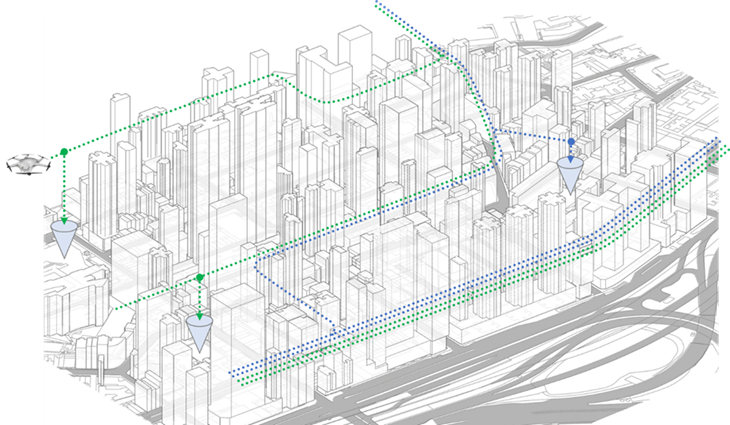
Figure 1: An imaginary scenario of urban air delivery route network

To support the tube-based operations, we develop a route network planning method to design routes (tubes) in a complex urban environment in this paper. In general, the design of a route network for drone deliveries includes 1) strategic design, 2) tactical design. The strategic design is mainly driven by business considerations, e.g. identifying areas with high demand, needing medical / emergency responses, or lacking other transportation infrastructure, to select the vertiport locations and the network types to best serve a market. This kind of network design is outside the scope of this work, which is expected to be decided before planning the routes as presented in this work. The tactical design focuses on path planning for drone operations considering operational constraints, such as air traffic management restrictions, safety requirements, public acceptance, noise ordinances, etc. The tactical design of a route network for drone operations in an urban environment is the focus of this work.

There are many existing path planning methods in the literature. However, to the best of our knowledge, none of them can be directly used to design a route network for urban air delivery at a city level due to the computational complexity involved in real-world scenarios. The problem of designing an optimal network with spatially separated routes is NP-hard (Yu & LaValle, 2013b). Path finding for one route is coupled with path finding for other routes. One route is planned with the shortest length (or the lowest cost), but other routes may need to take a significant detour to avoid any conflict, resulting in a sub-optimal solution at the system level. The computational complexity increases exponentially as the number of conflicts among routes increases. In addition, there is an unique requirement on the design of a drone delivery network in an urban area, which is the spread of a route network needs to be minimized to reduce the impact of high volume drone operations on safety, noise, and privacy, etc. Therefore, the routes in a network need to be aligned and close to each other as much as possible, which would reduce the total size of areas been affected by drone operations and increase the utilization of limited airspace in urban areas. The alignment of traffic flows would also decrease the traffic complexity in airspace and reduce the probability of separation loss (Hoekstra et al., 2018). However, no existing studies on path planning have considered network spread and airspace utilization.

To tackle these challenges, we propose a sequential path finding method to design a tube-based route network for drone operations in an urban environment considering airspace utilization. In this method, we propose a prioritization structure to decouple the network planning problem into a set of single-path planning problems to generate paths sequentially. We set the prioritization rules to rank origin-destination (OD) pairs to ensure important routes with higher priority in planning for better system performance. To obtain better airspace utilization, we introduce a space cost function in the underlying path-finding algorithm to build a network with dense and aligned routes. The contributions of this work are three folds:

• A sequential route network planning method with prioritization is developed to support tube-based operations for Unmanned Aerial Vehicles (UAVs) traffic management. The proposed prioritization framework can solve the NP-hard problem by decoupling the multi path-finding problem into sequential single path-finding problems to generate results fast.

• A new technique, referred to as space cost function, is developed to enable the design of dense route networks with improved airspace utilization.

• Comparative experiments and real-world applications are carried out to benchmark with other state-of-the-art methods and show the performance of the proposed method under various settings in real-world scenarios.

The remainder of this paper is structured as follows. An overview of related academic literature is provided in Section 2. The statement of the problem is illustrated in Section 3. The proposed method for route network planning is explained in Section 4. We evaluate the proposed method in testing scenarios and a real-world scenario in Section 5. Finally, Section 6 concludes the research findings and proposes future work.

2 Literature Review

On drone delivery problem, a large number of studies focuses on vehicle routing problem with drones (Shen et al., 2020) and traffic management problem for drones. The vehicle routing problems involve how to coordinate delivery trucks and drones to deliver small parcels to geographically distributed customers (Moshref-Javadi et al., 2020; Ha et al., 2018; Karak & Abdelghany, 2019; Murray & Chu, 2015; Murray & Raj, 2020; Sacramento et al., 2019; Schermer et al., 2019; Zhang et al., 2021). The traffic management problem is about how drones fly safely to finish tasks. It includes three steps. One is to plan a trajectory for each drone operation (Yang & Sukkarieh, 2008; Cekmez et al., 2014; Sonmez et al., 2015; Zhao et al., 2018; Wu et al., 2021), one is to detect conflicts when drones follow these trajectories (Tan et al., 2019; Islami et al., 2017; Kuchar & Yang, 2000), one is to resolve conflicts among drones if conflicts appear (Yang & Wei, 2020; Bertram et al., 2021; Yang & Wei, 2021; Tang et al., 2021).

In this paper, we focus on the problem of designing a network with multiple routes in an urban environment; each route connects an origin and a destination and is spatially separated from each other. Related studies can be broadly grouped in to two categories : the single-path finding (SPF) problem and the multi-path finding (MPF) problem.

2.1 Single-Path Finding

SPF involves moving a single agent to a destination among a set of obstacles. SPF is a well-studied area and many algorithms are proposed to find a path for the single agent.

Graph-search-based algorithms require a discretization of the state space, they search over the graph to find a path. The Dijkstra’s algorithm was the pioneer (Dijkstra, 1959; Liu et al., 2020), it searches the minimum cost paths between two points in the graph by comparing all possible combinations. A* is an advancement of the Dijkstra’s algorithm (Hart et al., 1968), it uses a heuristic function to estimate the cost of reaching the goal to reduce computational times. Many variants of A* were developed, like Dynamic A* (D*) (Koenig & Likhachev, 2005), Theta* (Daniel et al., 2010). For these methods, some solutions might be missed if the resolution of the discretization is large, and these methods do not guarantee to find an optimal path because of the heuristic nature, unless the heuristic is admissible, i.e., it never overestimates the cost of reaching the goal. In summary, these methods are efficient to find near-optimal paths with an appropriate resolution of the discretization in terms of the large size of the designing space.

Sampling-based algorithms do not require a discretization of the state space, they generate some possible paths by randomly adding points in the environment into a tree until some solution is found or time expires. Two prominent examples are Probabilistic Roadmap Method (PRM) (Kavraki et al., 1996) and Rapidly-Exploring Random Tree (RRT) (Lavalle, 1998). The PRM method first samples points in the environment and connect points to form a roadmap, and then it searches for a feasible path using this constructed roadmap. The RRT method grows a unidirectional search tree from the starting point until a tree branch hits the goal point. The RRT method guarantees finding a feasible solution as the number of iterations approaches infinity, however, the paths are often much longer than the optimal paths. Though its variant RRT* (Karaman & Frazzoli, 2011) is asymptotically optimal, the convergence rate is very slow. A comparison shows (Zammit & Van Kampen, 2018) that A*’s path length is more optimal and generation time is shorter than RRT for path planning for UAVs. In summary, sampling-based methods are still efficient to find a feasible path in terms of the large size of the designing space, but the path is extremely sub-optimal.

There are also some methods like mathematical optimization-based algorithms, neural network-based algorithms, nature-inspired algorithms. The mathematical optimization-based algorithms formulate the path finding problem as binary linear programming problems (Chamseddine et al., 2012) or mixed-integer programming problems (Culligan et al., 2007), and use high-quality solvers to solve these programming problems. Neural network-based algorithms (Yang & Meng, 2000; Dezfoulian et al., 2013; Singh & Thongam, 2019) use neural networks to model complex environments. Natural inspired algorithms, like genetic algorithms (Hu & Yang, 2004), particle swarm optimization (Masehian & Sedighizadeh, 2010), ant colony optimization (Englot & Hover, 2011) are also successfully applied for path finding. However, these methods are time consuming, they are not efficient to find a path in terms of the large size of the designing space.

In summary, if the size of the designing space is large, A* and its variants are the best choices considering computational time and the optimality of the path.

2.2 Multi-Path Finding

MPF involves navigating the agents to their respective targets while avoiding collisions with obstacles and other agents. Such problems are NP-hard (Yu & LaValle, 2013b). There are two different Multi-path finding problems based on the different cost function to minimize, one is sum-of-cost and another is makespan (Felner et al., 2017). For sum-of-cost problems, the sum of the total time steps or total distance for all agents should be minimized. For makespan problems, the maximum of the individual path costs should be minimized. Designing tube-based route networks is similar to the sum-of-cost problems, but there is a major difference that the sum-of-cost problems only require paths to be temporal conflict-free, but tube-based route networks further require paths to be spatial conflict-free, i.e., no path can appear at the same place even at different times.

Traditional MPF algorithms fall into two settings: centralized and distributed. In a distributed setting, each agent has its computing power and it does not have full knowledge of other agents. Some work has been done for the distributed setting (Bhattacharya et al., 2010; Gilboa et al., 2006; Grady et al., 2010). By contrast, the centralized setting assumes a single central computing power which needs to find a solution for all agents. The scope of this paper is limited to the centralized setting, thus here we provide a review on MPF algorithms in a centralized setting grouped into two categories: optimal solvers and sub-optimal solvers.

2.2.1 Optimal Solvers for Centralized MPF

The optimal solvers can generate optimal paths and they are complete in theory. However, the dimension of the problem explode exponentially as the number of agents increases. Thus, they are often used to generate routes for a small number of agents. These solvers can be broadly classified into A*-based, reduction-based, and two-level-based methods.

A* can be well suited to solve MPF sum-of-cost problems by taking k-agent state space. Each state includes k agents as a vector, e.g., in the start state each agent is located at its start point. For each state, there are $4^{k}$ neighbors to explore if each agent can move in four cardinal directions. Even for 10 agents, there are $4^{10}\approx 10^{6}$ neighbors for the start state. As a result, the original A*-based method is computationally infeasible to solve real-world problems. A few techniques are developed to speed up A*. For example, independence detection divides the agents into independent groups and solves these groups separately (Standley, 2010; Wagner & Choset, 2015), here two groups are independent if the optimal solution for each group does not conflict with the other. Another technique is related to surplus nodes, which are nodes generated but never be expanded to find an optimal solution. Avoiding generating the surplus nodes makes a substantial speedup (Standley, 2010; Felner et al., 2012; Goldenberg et al., 2014). In summary, though these techniques provide exponential speedup for A*-based methods, solution quality still degrades rapidly and computational time increases fast as the agent density increase.

Reduction-based methods reduce the MPF problem to standard known problems. Examples include network flow problems with integer linear programming formulations (Yu & LaValle, 2016, 2013a), Boolean satisfiability (Surynek, 2012), and constraint satisfaction problems (Ryan, 2010). These methods are designed for the MPF makespan problems, and they are inefficient or even inapplicable for MPF sum-of-cost problems.

Two-level-based methods introduce a tree structure to solve MPF sum-of-cost problems. Each node in the tree includes a solution for all routes, At the high level, these methods search over the tree to find the optimal solution, and then the low-level search is invoked to generate a node of the tree. Typical two-level-based methods include increasing cost tree search (Sharon et al., 2013) and conflict-based search (CBS) (Sharon et al., 2015). CBS is a state-of-the-art optimal solver. It uses a constraint tree (CT) for search. In a CT, each node includes a set of constraints on agents, a solution for all agents that satisfies the constraints, and the cost of the solution. The root node of the CT contains no constraint, and the paths in the solution are individually optimal if ignoring other agents. The tree is built progressively from root nodes to leaf nodes. In each step, the high-level search assigns a conflict as a constraint for an agent to satisfy. On the leaf nodes, all conflicts are solved, so the solutions are all feasible paths. The leaf node with the minimum cost has optimal paths. In summary, these methods are efficient and find optimal paths for small problems. If there are many agents and many conflicts to solve, their computational times also increase very fast.

2.2.2 Sub-Optimal Solvers for Centralized MPF

The sub-optimal solvers are commonly used to generate feasible routes quickly for a large number of agents for sum-of-cost problems. By decomposing the problem into several sub-problems, the computational time can be significantly reduced. But most of the time they can only find sub-optimal paths and, in some cases, completeness is sacrificed to improve time complexity. The sub-optimal solvers can be roughly classified as rule-based methods, search-based methods, and hybrid methods.

Rule-based solvers make specific agent-movement rules for different scenarios and they do not need massive search steps. They usually require special properties of the graphs to guarantee completeness. The algorithm by (Kornhauser et al., 1984) guarantees the completeness for all different graphs but the implementation is complex. BIBOX (Surynek, 2009) is complete for bi-connected graphs. Push-and-Swap (Luna & Bekris, 2011) uses ”swap” macro to swap locations between two adjacent dependent agents. Its variants Push-and-Rotate (De Wilde et al., 2014), Push-and-Spin (Alotaibi & Al-Rawi, 2018), etc., use more macros to handle complex situations and graphs. However, deadlocks often happen in narrow corridors and inter-agent collision-free may not be guaranteed, so the algorithms may fail to find paths even the paths exist (incompleteness). In summary, rule-based methods are efficient if there are a large number of agents, but the generated results are often far away from optimal.

Search-based methods search over the graph to find feasible solutions. The solutions are often near-optimal and sometimes but they are not complete for many cases. Prioritized approaches are a kind of prominent search-based methods. They plan routes sequentially and treat positions of previously planned agents as moving obstacles to avoid any collision (Van Den Berg & Overmars, 2005). Hierarchical Cooperative A* (HCA*) (Silver, 2005) is a typical prioritized approach. HCA* plans one route for one agent at a time according to a predefined order, and it stores each route into a reservation table after the route is planned. The previous paths, i.e., entries in the reservation table, are impassable for later agents. Windowed HCA* (WHCA*) (Silver, 2005) runs in a similar way but it uses plan-move cycles to dynamically generate routes. In each planning phase, each agent reserves the next W steps by the order; in each moving phase, each agent follows the reserved paths by K ($K\leq W$) steps, then the next cycle starts in the current point. Conflict-oriented WHCA* (CO-WHCA*) (Bnaya & Felner, 2014) places the window, i.e., the reservation for the next W steps, only around conflicts. The choice of priorities has a great impact on the performance of planned routes (Warren, 1990) and there exist different strategies. Arbitrary order is applied in HCA* and the planning phase in each cycle in WHCA*. The decreasing order of the shortest path length for each agent is taken as the criterion in (Van Den Berg & Overmars, 2005). A winner-determination strategy is taken in CO-WHCA*, where all possible orders are estimated for every conflict and the best one is selected. Several search-based methods are bounded sub-optimal solvers (Barer et al., 2014; Cohen et al., 2019, 2016). Most of them are variants of conflict based search, they provide bounded sub-optimal solutions by relaxing the assumptions and conditions. In summary, prioritized approaches provide near-optimal solutions and they are still efficient when there are many agents. Bounded sub-optimal methods improve computational time compared to optimal methods, but they are still not efficient for a large number of agents.

Hybrid methods take both specific agent-movement rules and massive search steps. In the first phase, a path is planned for each agent individually with obstacle avoidance by using SPF algorithms while other agents’ paths are ignored at this phase. In the next phase, the agents coordinate to ensure no inter-agent collision occur along the paths. Common coordination methods include modification of geometric paths, modification of velocity profiles, and delay in the startup time of agents (Kant & Zucker, 1986; Leroy et al., 1999; Li et al., 2005; O’Donnell & Lozano-Pérez, 1989; Peng & Akella, 2005; Saha & Isto, 2006; Sanchez & Latombe, 2002). These coordination schemes are the rules for solving conflicts. In summary, these methods can find paths fast if there are many agents, but most of them use time dimension to avoid collision and they cannot guarantee paths are spatial conflict-free.

In summary, none of the existing multi-path finding methods can readily solve the route network planning problem in this paper. The problem is NP-hard. The search space for the drone network design is large considering the size of the design space, cluttered obstacles, complexity of risk levels, and the coupled complexity of many routes to be planned. The optimal solvers are inefficient to solve the problem as it suffers the curse of dimensionality. Rule-based sub-optimal methods and hybrid sub-optimal methods are much efficient, but their solutions are often too far away from optimal. Also, they require to use the time dimension to solve conflicts. Spatial intersections may still exist in the generated network. Prioritized approaches are applicable and efficient, and their results are near-optimal. Therefore, following the prioritized approaches, we develop a set of prioritization rules and integrate them into a sequential route planning algorithm for drone route network planning in an urban environment in this paper.

3 Problem Statement

This section defines the drone delivery network that we aim to design. An illustration of the network is shown in Figure 2. Air routes are unidirectional paths established among approaching and departing fixes over Origin-Destination vertiports. Drones can fly sequentially in a path following the minimum spacing requirement. The width and height of a path are 20 meters and 10 meters, which is determined based on drone position uncertainties and measurement errors. There is a layer of airspace surrounding the path that serves as ”buffer zones” with a width of 10 m, as shown in Figure 3. No other path or obstacle is allowed in the buffer zone, and the vertical and horizontal separation requirements are shown in Figure 3 and Figure 4. However, the buffer zones of different paths can be overlapped as shown in Figure 3.

For the design of a route network, individual paths are expected to expose minimum risks to the ground and to impose minimum energy consumption of drone operations. On a network level, the spread of the route network should be minimized. Besides, the computational time for generating a route network should also be short.

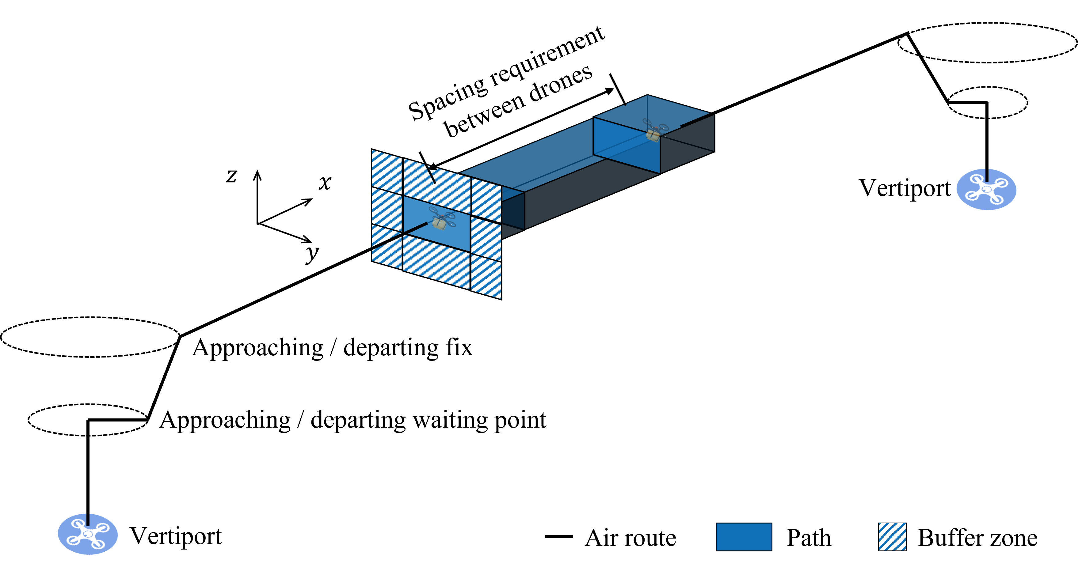
Figure 2: Components of a route network

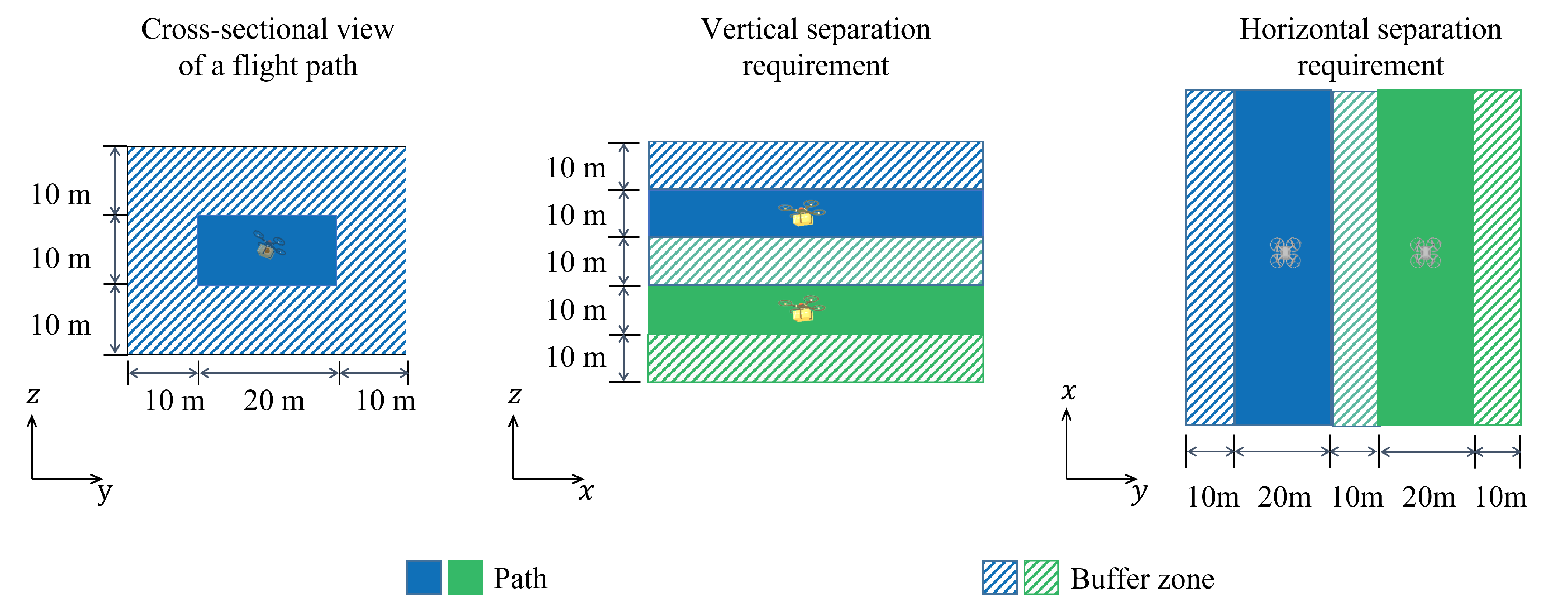
Figure 3: Dimension of a flight path and its separation requirement

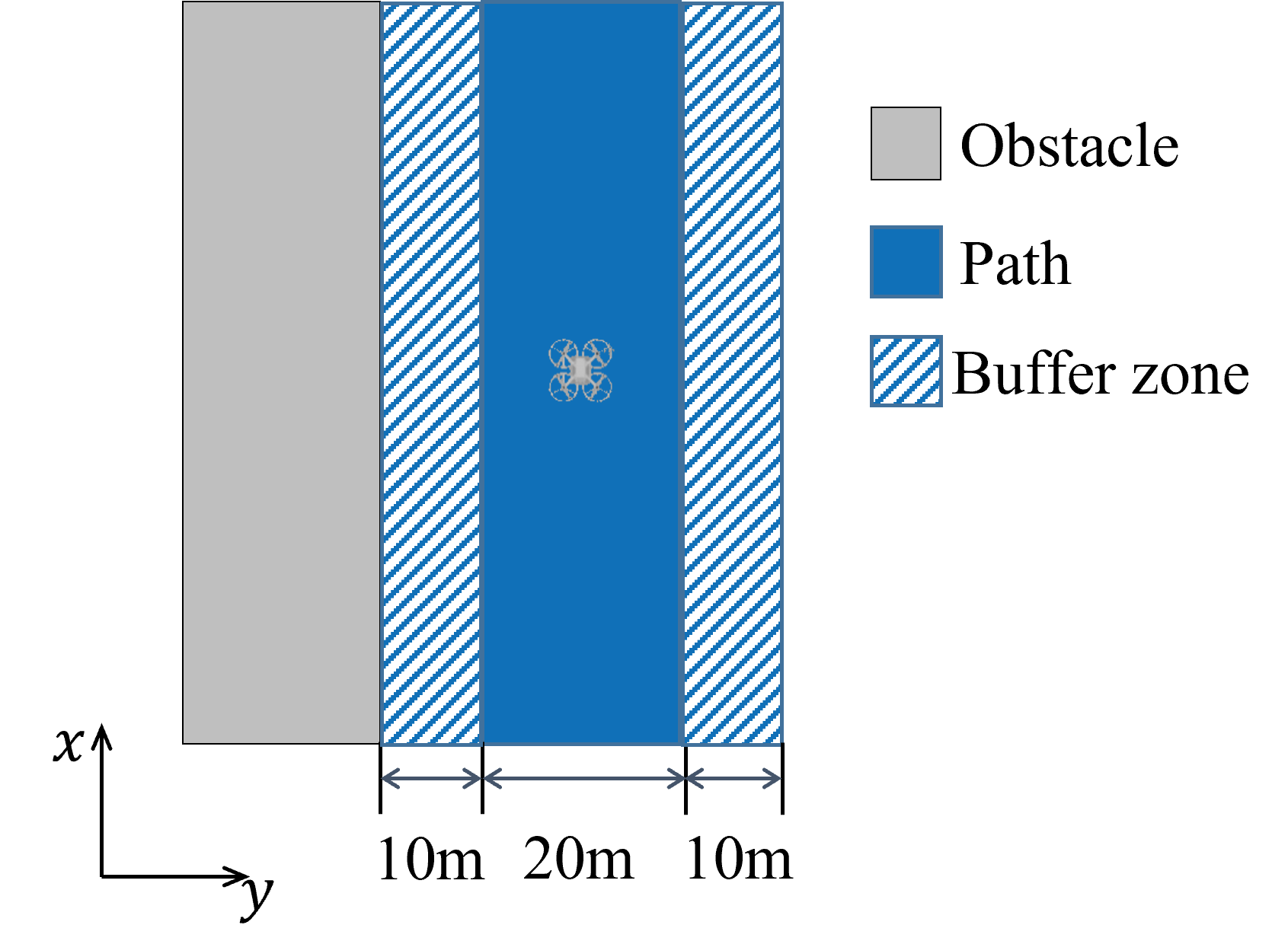
Figure 4: Separation requirement between a path and an obstacle

4 Methodology for Route Network Planning

4.1 Overview

To design a route network for an urban area as described in Section 3, we develop a novel sequential route network planning method considering airspace utilization. In this method, we propose a prioritization structure to decouple the network planning problem into a set of single-path planning problems to generate paths sequentially. We set the prioritization rules to rank origin-destination (OD) pairs to ensure important routes with higher priority in planning for better system performance. To obtain better airspace utilization, we introduce a space cost function in the underlying path-finding algorithm to build a network with dense and aligned routes.

The proposed route network planning method is composed of four modules: Environment Discretization, Individual Route Planning, Route Prioritization, and Network Planning. The Environment Discretization module generates graphs for searching, the Route Prioritization module generates multiple ordered route sequences, and the Network Planning module generates route networks based on the graphs and the route sequences. In generating a route network, the Individual Route Planning module is iteratively conducted to generate a route network for each route sequence. The Network Evaluation module selects the route network that has a minimum cost from all generated route networks, then it checks the risk for each path in the selected route network. If all paths satisfy the risk requirement, the selected route network will be returned as the final route network; otherwise, the method fails to find a feasible route network. The overall workflow is illustrated in Figure 5. The associated algorithm, named as Sequential Extended Theta* with Route Prioritization and Space Cost, is shown in Algorithm 1.

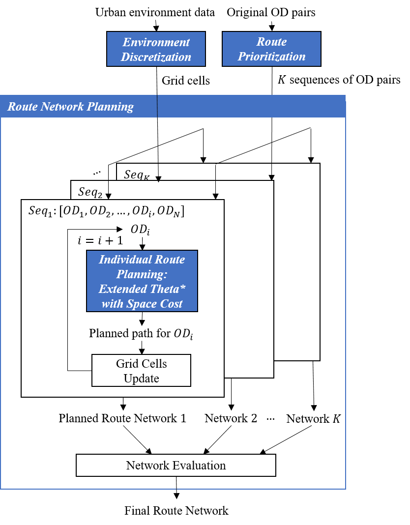
Figure 5: Overall workflow of the proposed route network planning method

Input : OD pairs $\{OD_{i}\}_{i=1}^{N}$, environment $E$

Output : A route network $\{R_{i}\}_{i=1}^{N}$

1 /* Environment Discretization */

2 Perform space discretization on $E$;

3 Generate grid cells to compose graph $G(V,E)$;

4 /* Route Prioritization */

5 Generate $K$ OD pair sequences $\{Seq_{k}\}_{k=1}^{K}$from original OD pairs $\{OD_{i}\}_{i=1}^{N}$;

6 /* Network Planning */

7 for $Seq_{k}$ in $\{Seq_{k}\}_{k=1}^{K}$ do

8       for $OD_{i}$ in $Seq_{k}$ do

9             /*Individual planning*/

10             Run Extended Theta* with Space Cost on $OD_{i}$ to get planned paths $R_{i}^{k}$;

11             /*Update grid cells*/

12             Set path cells for $R_{i}^{k}$ as unreachable (impassable for obstacles and $R_{j>i}^{k}$);

13             Set buffer zone cells for $R_{i}^{k}$ as reserved (impassable for obstacles and paths of $R_{j>i}^{k}$, passable for buffer zones of $R_{j>i}^{k}$);

14       end for

15      Store the route network $\{R_{i}^{k}\}_{i=1}^{N}$;

16 end for

17/* Network Evaluation */

18 Find $\{R_{i}\}_{i=1}^{N}$ with lowest costs from $K$ route networks $\{\{R_{i}^{k}\}_{i=1}^{N}\}_{k=1}^{K}$

19 Check risk for each path;

20 if a subset of the paths do not satisfy the risk requirement then

21       return ”fail to generate a feasible route network”

22else

23       Return the route network $\{R_{i}\}_{i=1}^{N}$

24 end if

25

Algorithm 1 Route Network Planning: Sequential Extended Theta* with Route Priority and Space Cost

4.2 Environment Discretization

This module aims to generate a grid graph for the network planning. It discretizes the environment into 3D cubic grid cells to compose a grid graph $G(V,E)$. The process is shown in Figure 6.

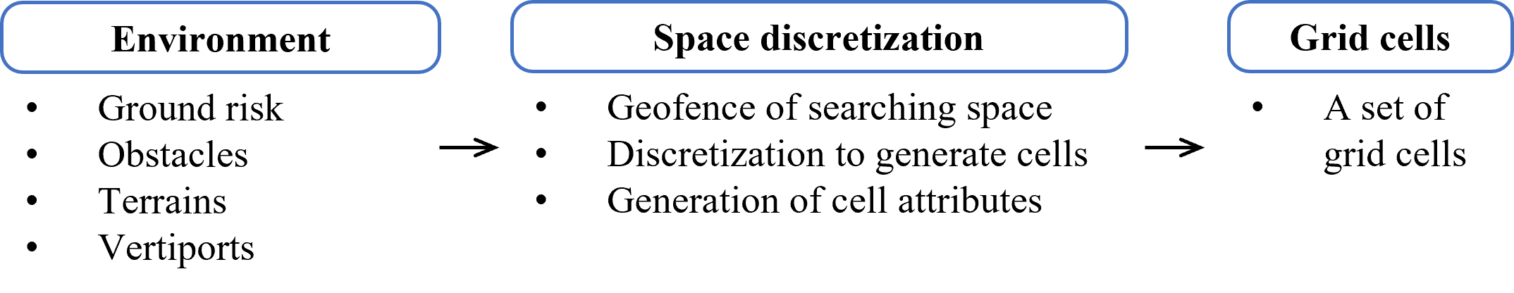
Figure 6: Flowchart of environment discretization

The environment includes ground risk, obstacles, terrains, and vertiports. They are processed as different layers, as shown in Figure 7. These layers are used to generate attribute values for each cell in the next discretization process. The risk layer specifies areas with high/low risks. It is calculated based on many factors, e.g., population density, sheltering factor, critical infrastructures, noise impact, public acceptance, etc. The calculation is outside the scope of this work. The obstacle/terrain layer includes obstacles like buildings, trees, no-fly zones, and terrains like flat ground and mountains. Drones should avoid any collision with obstacles and terrains. The vertiport layer provides taking off and landing points for drones.

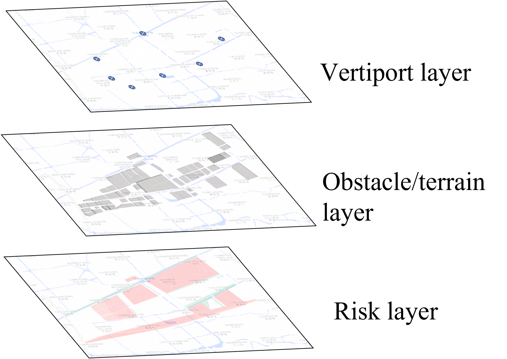
Figure 7: Environment layers

The space discretization process first discretizes the environment into 3D cubic grid cells, then it determines the attributes of each cell based on environment layers. Each environment layer determines the value of an attribute of a cell. The vertiport layer determines whether a cell is an origin/destination vertiport or not, the obstacle/terrain layer determines whether a cell is passable or not, and the risk layer determines what is the ground risk level associated with each cell. These grid cells compose the grid-graph $G(V,E)$ for the following network planning.

4.3 Individual Route Planning: Extended Theta* with Space Costs

This module aims to find a conflict-free path for each OD pair that minimizes drones’ energy consumption, the potential risk to ground, and airspace occupancy. The underlying algorithm for this module is referred to as extended Theta* with space cost in this paper. The pseudo-code of this algorithm is shown in Algorithm 2. The basic idea of this algorithm is explained below.

The proposed path planning algorithm, extended Theta* with space cost, is developed based on the most commonly used graph-based search algorithms, A* (Hart et al., 1968) and its variant Theta* (Daniel et al., 2010). In both A* and Theta*, the algorithm searches a path from a start node $s_{start}$ to a destination node $s_{goal}$ that has minimum total cost $g(s_{start},s_{goal})$. In the path searching process, the algorithm starts from the start node $s_{start}$, iteratively explores a set of nodes and determine which one would be the best as the next node to generate a path in the end. Instead of searching and evaluating all nodes in the graph, a heuristic is used to guide the algorithm to extend nodes towards the destination. The heuristic is based on the cost required to extend the path all the way to the goal, which is estimated by the direct distance from the node to the goal. If a node has a higher heuristic cost, it will be less likely to be included in the path. Specifically, in the search process of a path, to extend a node $s$ from a node $s^{{}^{\prime}}$ towards the destination node, A* minimizes a cost function $f(s_{start},s)$, which is based on the total cost of the path $g(s_{start},s)$ and the heuristic $h(s,s_{goal})$, i.e.,

$$f(s_{start},s)=g(s_{start},s)+h(s,s_{goal}).$$ (1)

An illustration for the A* path finding is shown in Figure 8.

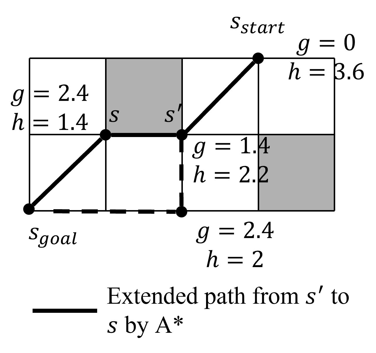
Figure 8: Illustration of A* path finding

In this paper, we modify the cost function $g$ to design each route that minimizes drones’ energy consumption, the potential risk to ground, and airspace occupancy, as shown in E.q. (2).

$$g(s_{start},s_{goal})=o(s_{start},s_{goal})+\omega_{r}r(s_{start},s_{goal})+\omega_{p}p(s_{start},s_{goal}).$$ (2)

In this formula, $o(s_{start},s_{goal})$, $r(s_{start},s_{goal})$, and $p(s_{start},s_{goal})$ are operational cost, risk cost, and space cost; $\omega_{r}$ and $\omega_{p}$ are weight coefficients. Aside from these cost functions, a few other operational constraints might affect the route network design, such as public acceptance, noise ordinances, air traffic restrictions, etc. These operational constraints can be considered using the cost factors in a similar way. $\omega_{r}$ and $\omega_{p}$ in E.q. (2) reflect the relative importance of risks and airspace utilization in comparison with drone flying time and energy consumption. The values can be determined by the relative monetary cost of the different categories. For example, the operational cost can be estimated by the time value of the drone delivery service and the cost of energy. The economic cost of a drone crash on ground can be estimated to gauge the risk weight value. The weight value of airspace utilization can be calculated based on the airspace usage charges or other urban airspace regulations to be established in the future.

The operational cost captures flying distance and the energy consumption for drone operations, including traversing a distance, turning, and climbing/descending. For a set of path segments $\{\textbf{\em l}_{i}\}_{i=1}^{n}$ that connects $s_{start}$ and $s_{goal}$, the operational cost is calculated as

$$o(s_{start},s_{goal})=traversal(s_{start},s_{goal})+turning(s_{start},s_{goal})+climbing(s_{start},s_{goal})+descending(s_{start},s_{goal}),$$ (3)

where

$$traversal(s_{start},s_{goal})=\sum_{i=1}^{n}\left\|\textbf{\em l}_{i}\right\|,$$ (4)

$$turning(s_{start},s_{goal})=\lambda_{turning}\sum_{i=1}^{n-1}\left|arccos(\frac{\textbf{\em l}_{i}\cdot\textbf{\em l}_{i+1}}{\left\|\textbf{\em l}_{i}\right\|\left\|\textbf{\em l}_{i+1}\right\|})\right|,$$ (5)

let $\textbf{\em n}=[0,0,1]^{T}$, then

$$climbing(s_{start},s_{goal})=\lambda_{climbing}\sum_{i=1}^{n}max(arcsin(\frac{\textbf{\em l}_{i}\cdot\textbf{\em n}}{\left\|\textbf{\em l}_{i}\right\|}),0)\left\|\textbf{\em l}_{i}\right\|,$$ (6)

$$descending(s_{start},s_{goal})=\lambda_{descending}\sum_{i=1}^{n}max(-arcsin(\frac{\textbf{\em l}_{i}\cdot\textbf{\em n}}{\left\|\textbf{\em l}_{i}\right\|}),0)\left\|\textbf{\em l}_{i}\right\|.$$ (7)

Here $\lambda_{turning},\lambda_{climbing},\lambda_{descending}$ are coefficients to normalize energy consumption for different drone operations.

The risk cost captures the potential risk to the ground, it reflects various risk levels by accumulating the risks involved in passing through the cells. It is calculated as

$$r(s_{start},s_{goal})=\lambda_{r}\sum_{s_{start}}^{s_{goal}}\theta_{risk},$$ (8)

where $\theta_{risk}$ indicates the risk level of an area. Areas that are densely populated or with critical infrastructures have higher risk levels, with $\theta_{risk}>1$; areas that are not populated and with less ground impact concerns have lower risk levels, with $0<\theta_{risk}<1$; most areas are set to have a normal risk level, with $\theta_{risk}=1$. $\lambda_{r}$ is a scaling factor for raw risk cost, the calculation of it is in Appendix A.

The space cost function encourages bundled paths and overlapped buffer zones to improve airspace utilization. An illustration is shown in Figure 9. The size of buffer zones in Figure 9(a) and Figure 9(b) are the same and equal to the required minimum separation. In Figure 9(a), the buffer zones of two aligned paths are not overlapped and the separation between the paths is twice the required minimum separation; in Figure 9(b), the buffer zones are overlapped and the separation between the paths is exactly the required minimum separation. For a path between cell $s_{start}$ and cell $s_{goal}$, the space cost item $p(s_{start},s_{goal})$ measures the marginal volume of occupied airspace, i.e.,

$$p(s_{start},s_{goal})=\lambda_{p}N(s_{start},s_{goal}),$$ (9)

here $\lambda_{p}$ is a scaling factor for raw space cost, the calculation of it is in Appendix A, $N(s_{start},s_{goal})$ is calculated by

$$N(s_{start},s_{goal})=N_{path}(s_{start},s_{goal})+N_{new\_{buf}}(s_{start},s_{goal}),$$ (10)

where $N_{path}$ is the increased number of path cells by adding a path between cell $s_{start}$ and cell $s_{goal}$ to the existing network, while $N_{new\_{buf}}$ is the increased number of buffer zone cells by adding a path between cell $s_{start}$ and cell $s_{goal}$ to the existing network. Taking Figure 9 as an example, buffer zones in Figure 9(a) do not overlap, so all buffer zone cells are newly introduced. For the situation in Figure 9(b), when planning a path $r_{2}$ after path $r_{1}$ has been planned, some of $r_{2}$’s buffer zone cells overlapped with the buffer zones of $r_{1}$. These buffer zone cells will not be counted again in $N_{new\_{buf}}$ for $r_{2}$. After the addition of the space cost function, the total cost reduces but the length of paths increases, but this is not an issue. As a drone delivery operator, the cost is associated with the direct drone operations as well as the airspace usage charges, similar to the airline operations.

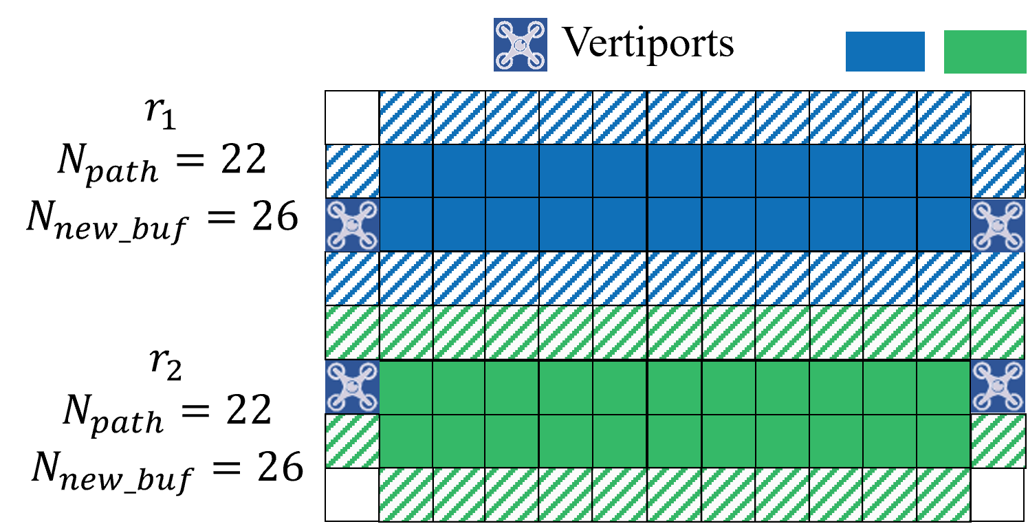
(a) buffer zones do not overlap

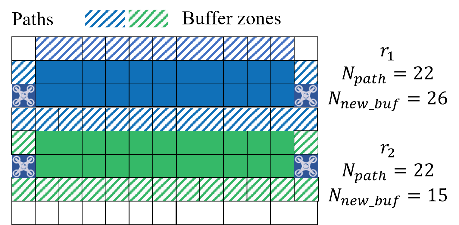
(b) buffer zones overlap

Figure 9: An illustration for overlapping buffer zones (top view)

To ensure the effectiveness of the space cost function for the purpose of reducing total costs, the relative value of the space cost weight coefficient $\omega_{p}$ in relation to other cost coefficients needs to be carefully calibrated to reflect the actual operational cost impact of airspace usage charges. For example, when the space cost weight coefficient $\omega_{p}$ is small, the space cost has little impact on route density. As $\omega_{p}$ increases, the algorithm starts to reduce large space costs at the expense of a small increase in other costs. When $\omega_{p}$ is large, the algorithm generates a network where paths are heavily bundled to have more overlapped buffer zones, but the paths may pass through areas with high operational cost and risk cost.

1 Main():

2       $open:=closed:=\emptyset$

3       $g(s_{start},s_{start}):=0$

4       $parent(s_{start}):=s_{start}$

5       $open.Insert(s_{start},g(s_{start},$

6       $s_{start})+h(s_{start},s_{goal}))$

7       while $open\neq\emptyset$ do

8             $s^{{}^{\prime}}:=open.Pop()$

9             [SetVertex($s^{{}^{\prime}}$)]

10             if $s^{{}^{\prime}}=s_{goal}$ then

11                   return ”path found”

12             end if

13            $closed:=closed\cup\{s^{{}^{\prime}}\}$

14             foreach $s\in nghbr_{vis}(s^{{}^{\prime}})$ do

15                   if $s\notin closed$ then

16                         if $s\notin open$ then

17                               $g(s_{start},s):=\infty$

18                               $parent(s):=NULL$

19                              

20                         end if

21                        UpdateVertex($s^{{}^{\prime}},s$)

22                   end if

23                  

24             end foreach

25            

26       end while

27      return ”no path found”

28

29

30UpdateVertex($s^{{}^{\prime}},s$):

31       $g_{old}:=g(s_{start},s)$

32       ComputeCost($s^{{}^{\prime}},s$)

33       if $g(s_{start},s)<g_{old}$ then

34             if $s\in open$ then

35                   $open.Remove(s)$

36             end if

37            $open.Insert(s,g(s_{start},s)+h(s,s_{goal}))$

38       end if

39      

40

41 SpaceCost($s^{{}^{\prime}},s$):

42       /* calculate space cost

43       traveling from $s^{{}^{\prime}}$ to $s$ */

44       $N(s^{{}^{\prime}},s)=N_{path}(s^{{}^{\prime}},s)+N_{new\_pro}(s^{{}^{\prime}},s)$

45       $p(s^{{}^{\prime}},s)=\lambda_{p}N(s^{{}^{\prime}},s)$

46       return $p(s^{{}^{\prime}},s)$

47

48 ComputeCost($s^{{}^{\prime}},s$):

49       if $lineofsight(parent(s^{{}^{\prime}}),s)$ then

50             /* Path 2 */

51             $\color[rgb]{1,0,0}p(parent(s^{{}^{\prime}}),s)=SpaceCost(parent(s^{{}^{\prime}}),s)$

52             $g(parent(s^{{}^{\prime}}),s)=o(parent(s^{{}^{\prime}}),s)+\omega_{r}r(parent(s^{{}^{\prime}}),s)+\color[rgb]{1,0,0}\omega_{p}p(parent(s^{{}^{\prime}}),s)$

53             if $g(s_{start},parent(s^{{}^{\prime}}))+g(parent(s^{{}^{\prime}}),s)<g(s_{start},s)$ then

54                   $parent(s):=parent(s^{{}^{\prime}})$

55                   $g(s_{start},s):=g(s_{start},parent(s^{{}^{\prime}}))$

56                  $+g(parent(s^{{}^{\prime}}),s)$

57                  

58             end if

59            

60       else

61             /* Path 1 */

62             $\color[rgb]{1,0,0}p(s^{{}^{\prime}},s)=SpaceCost(s^{{}^{\prime}},s)$

63             $g(s^{{}^{\prime}},s)=o(s^{{}^{\prime}},s)+\omega_{r}r(s^{{}^{\prime}},s)+\color[rgb]{1,0,0}\omega_{p}p(s^{{}^{\prime}},s)$

64             if $g(s_{start},s^{{}^{\prime}})+g(s^{{}^{\prime}},s)<g(s_{start},s)$ then

65                   $parent(s):=s^{{}^{\prime}}$

66                   $g(s_{start},s):=g(s_{start},s^{{}^{\prime}})+g(s^{{}^{\prime}},s)$

67                  

68             end if

69            

70       end if

71      

72

Algorithm 2 Extended Theta* with Space Cost

4.4 Route Prioritization and Network Planning

This module specifies the prioritization framework based on a set of prioritization rules to rank the importance of routes and decouple the network planning problem into sequential planning. As discussed in the introduction, the network-planning problem is an NP-hard problem. An optimal solution of a single path occupies certain airspace, which may force other paths to detour. Thus, a change of one path affects all other paths. In this paper, we use a simple but effective strategy to decouple the network planning problem into a set of single-path planning problems - plan the paths one by one from the most important to the least important.

In this module, a prioritization structure with example rules is proposed. These rules can be changed depending on specific business considerations. The prioritization structure is shown in Figure 10. There can be multiple levels to prioritize the paths. Level $l_{0}$ has the sequence of original OD pairs and it is grouped into a series of subsequences by the most important priority rule, $R_{1}$. Then the subsequences on Level $l_{1}$ can be further grouped into subsequences by the second important priority rule, $R_{2}$. The paths in the subsequences on the bottom level are randomly shuffled to find the optimal sequence that generates the best network performance.

Figure 10: Illustration of the prioritization framework

To give a more detailed example, suppose we have two priority rules as specified below:

$$R_{1}=\{PL\},$$ (11)

$$R_{2}=\{v,\varepsilon_{v}\},$$ (12)

where $PL$ denotes the urgency level of paths, detailed as $\{Urgent,Important,Normal,Low\}$ ; $v$ is the expected profit value of each path and $\varepsilon_{v}$ is segment threshold of $v$. More priority rules can be taken to get more subsequences.

$R_{1}$ generates four subsequences $\{S_{i}\}_{i=1}^{4}$ directly based on urgency levels in $PL$. These subsequences are $(S_{Urgent},$ $S_{Important},S_{Normal},S_{Low})$, each of them represents an urgency level. $R_{2}$ sorts paths within each subsequence $S_{i}$ in $l_{1}$ by the expected profit value $v$ (in descending order), and generates a new set of subsequences $\{S_{ij}\}_{j=1}^{M_{i}}$, where $M_{i}$ is the number of subsequences in $S_{i}$. $\varepsilon_{v}$ divides each $S_{i}$ into a set of subsequences $\{S_{ij}\}_{j=1}^{M_{i}}$ based on the expected profit value distribution (Figure 11), similar to generating clusters based on density in DBSCAN (Ester et al., 1996). Given a set of paths with different $v$, OD pairs are grouped together with similar $v$ values. Each $S_{ij}$ satisfies the following property:

$$|v_{r}-v_{r^{{}^{\prime}}}|\leq\varepsilon_{v},\forall r,r^{{}^{\prime}}\in S_{ij}.$$ (13)

Paths in the subsequences on the bottom level are randomly shuffled to find the optimal sequence that generates the best network performance.

Figure 11: Illustration of the segmentation and shuffle in $R_{2}$

To balance between optimality and computational time, we randomly generate $K$ sequences following the above priority structure, where $K$ is a parameter that one can adjust. It can be adjusted in the range $[1,S_{g}]$,

$$K\in\mathbb{Z}:1\leq K\leq S_{g}.$$ (14)

$$S_{g}=\prod_{i=1,2,3,4}\prod_{j=1,2,...,M_{i}}n(S_{ij})!,$$ (15)

where $n(S_{ij})$ is the number of OD pairs in sub-sequence $S_{ij}$ , $n(S_{ij})!$ is the number of permutations in sub-sequence $S_{ij}$, and $S_{g}$ is the number of all possible ordered arrangements of OD pairs satisfying $R_{1}$ and $R_{2}$.

The complete strategy for determining route sequence order is shown in Algorithm 3. If there are two networks that generate the same performance in terms of the total costs, the algorithm will generate both networks and their associated costs in different categories. It’s up to the user to select which one to use based on the information of different cost categories and other considerations not captured in the model.

Input : Original OD pairs $\{OD_{i}\}_{i=1}^{N}$

Output : Ordered OD pairs $\{OD_{i}^{{}^{\prime}}\}_{i=1}^{N}$

1 /* Rule 1: get $\{S_{i}\}^{4}_{i=1}$, i.e., $(S_{Urgent},$ $S_{Important},S_{Normal},S_{Low})$ */

2 $\{S_{i}\}^{4}_{i=1}\leftarrow\emptyset$

3 for $r$ in $\{OD_{i}\}_{i=1}^{N}$ do

4       $S_{l}.append(r)$ if $r.PL==l$

5      

6 end for

7$\{S_{i}\}^{4}_{i=1}\leftarrow\{S_{l}\}$

8 /* Rule 2: get $\{\{S_{ij}\}_{j=1}^{M_{i}}\}^{4}_{i=1}$*/

9 for $S_{i}$ in $\{S_{i}\}^{4}_{i=1}$ do

10       Sort $S_{i}$ in descending order of $v$;

11       $\{S_{ij}\}_{j=1}^{M_{i}}\leftarrow$ subgroups from DBSCAN with $\varepsilon_{v}$ in $S_{i}$;

12       for $S_{ij}$ in $\{S_{ij}\}_{k=1}^{M_{i}}$ do

13             $S_{ij}\leftarrow$ random shuffled $S_{ij}$;

14            

15       end for

16      

17 end for

18

19 $\{OD_{i}^{{}^{\prime}}\}_{i=1}^{N}\longleftarrow\{\{S_{ij}\}_{j=1}^{M_{i}}\}^{4}_{i=1}$;

return $\{OD_{i}^{{}^{\prime}}\}_{i=1}^{N}$

Algorithm 3 Route Prioritization

5 Testing

In this section, we first use an illustrative scenario to show how the algorithm works. Then we compare the proposed algorithm with other path finding algorithms in a test scenario. After that, the proposed algorithm is applied to a real-world scenario in Hangzhou, China. In this real-world scenario, we show a set of sensitivity analyses on algorithm parameters and provide an empirical analysis of computational time.

5.1 Illustration with a Toy Example

In this section, we use a toy example to show how the space cost function improves airspace utilization for the network design. We apply the our method with space cost algorithm and the our method without space cost algorithm on the toy example shown in Figure 12. In this example, there are two symmetric obstacles and 10 vertiports (id 1-10).

In Experiment 1, both algorithms are applied to find three paths from upper vertiports to lower vertiports (id 3-8, 2-7, 4-9). The results are shown in Figure 12. If the space cost function is not added to the algorithm, three paths (①, ②, ③) will appear on the different sides of the obstacles to achieve a shorter distance, as shown in Figure 12(a); if the space cost function is added to the algorithm, three paths all appear in the middle of two obstacles and share the buffer zones, as shown in Figure 12(b). After adding the space cost function into the algorithm, the generated network occupies fewer buffer zones (16.7%) at the cost of slightly more path cells (4.8%), and the total occupied airspace reduces (6.7%), as shown in Table 1.

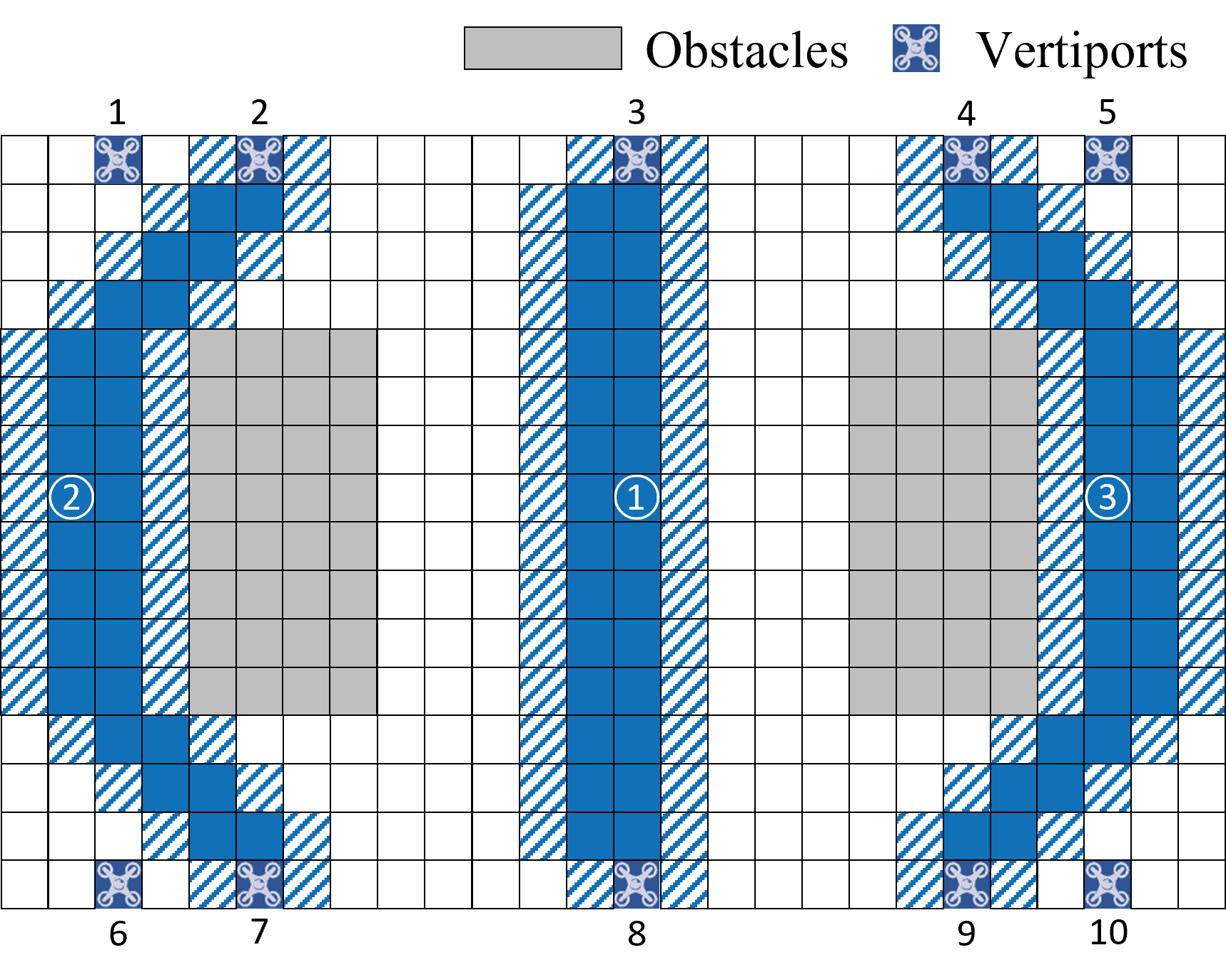
(a) Our method without space cost

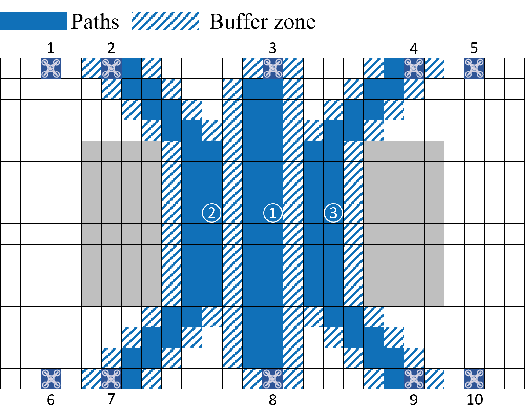
(b) Our method with space cost

Figure 12: A test case (top view) for network planning (a) without space cost and (b) with space cost

Table 1: Summary of planning three paths in the scenario

	# of buffer zone cells	# of path cells	Total occupied airspace
Our method without space cost	96	84	180
Our method with space cost	80	88	168
Improvement after adding space cost	16.7%	-4.8%	6.7%

In Experiment 2, both algorithms are applied to find five paths from upper vertiports to lower vertiports (id 3-8, 2-7, 4-9, 1-6, 5-10). The results are shown in Figure 13. When not adding the space cost function, the method fails to find the paths ④ and ⑤ because their traversable airspaces are blocked by the buffer zones of the paths ② and ③. By contrast, when adding the space cost function, the method successfully generates the extra paths (④, ⑤).

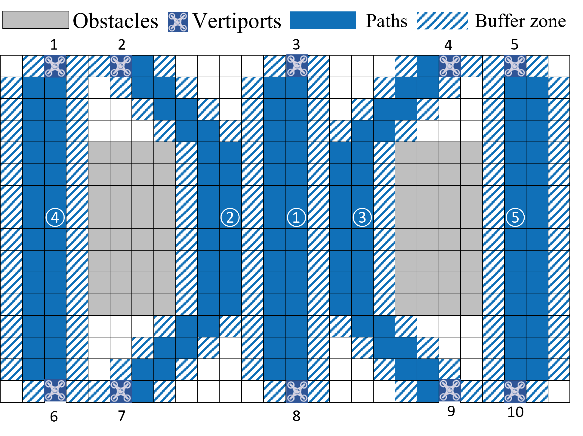
Figure 13: A test case (top view) of network planning with 5 paths

5.2 Comparisons with Other Algorithms on a 2D Scenario

In this section, we compare the proposed sequential route network planning method with two kinds of state-of-the-art MPF algorithms on a 2D standard test scenario: one is a two-level-based optimal method - conflict-based search (CBS) (Sharon et al., 2015), and one is a rule-based sub-optimal method - Push-and-Spin (Alotaibi & Al-Rawi, 2018). The scenario is shown in Figure 14. This scenario (Sturtevant, 2012) contains 65536 pixels/cells, and 6528 cells are inaccessible. Multiple OD pairs need to be planned in this experiment. The origins are located in the lower-left corner and the destinations are located in the upper-right corner.

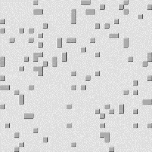
Figure 14: The 2D standard test scenario (Sturtevant, 2012)

Results show that the proposed method is capable to solve large scenarios within a reasonable amount of time. The comparisons are shown in Table 2. Both Push-and-Spin and the proposed method find paths quickly, while CBS cannot find paths in a reasonable time as the number of routes increases. The proposed method also shows an advantage in airspace utilization compared to CBS and Push-and-Spin. The paths generated by these algorithms are shown in Figure 15.

Table 2: Route network planning results of three methods in the 2D standard test scenario

# of routes	1	2	3	4	5	6	7	8	9	10	11	12	13	14	15	16	17	18	19	20
CBS
$sum\ of\ distance$	245	477	703	956	1203	1443	1694	1965	2263	-	-	-	-	-	-	-	-	-	-	-
# of occupied cells	1007	1923	2910	3965	4894	5918	6902	7993	9189	-	-	-	-	-	-	-	-	-	-	-
$time(s)$	0.02	0.03	1.98	134.04	1201.34	2029.10	2378.24	2836.76	3165.76	-	-	-	-	-	-	-	-	-	-	-
Push-and-Spin
$sum\ of\ distance$	245	477	707	966	1203	1466	#	#	#	#	#	#	#	#	#	#	#	#	#	#
# of occupied cells	1007	1923	2852	3904	4894	5877	#	#	#	#	#	#	#	#	#	#	#	#	#	#
$time(s)$	0.02	0.03	0.04	0.04	0.05	0.06	#	#	#	#	#	#	#	#	#	#	#	#	#	#
The proposed method
$sum\ of\ distance$	247	486	715	969	1226	1495	1734	1999	2266	2564	2893	3175	3490	3807	4087	4367	4666	4968	5316	5664
# of occupied cells	881	1491	2019	2771	3458	4121	4915	5699	6623	7400	8232	8949	9713	10522	11170	11867	12623	13349	14229	15311
$time(s)$	0.16	0.21	0.26	0.32	0.42	0.52	0.58	0.67	0.77	0.85	0.92	0.97	1.03	1.09	1.12	1.16	1.21	1.25	1.29	1.33

1. exceed the timeout limit (3600s)

2. unable to find feasible solutions

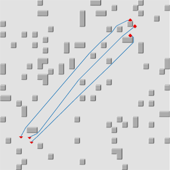
(a) 3 routes - CBS

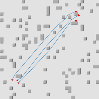
(b) 3 routes - Push-and-Spin

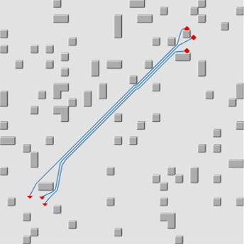
(c) 3 routes - The proposed method

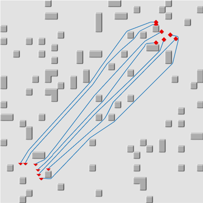
(d) 7 routes - CBS

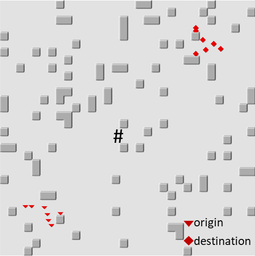
(e) 7 routes - Push-and-Spin

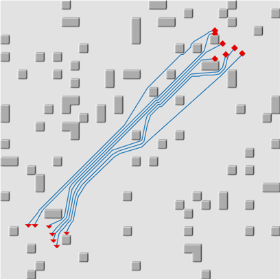
(f) 7 routes - The proposed method

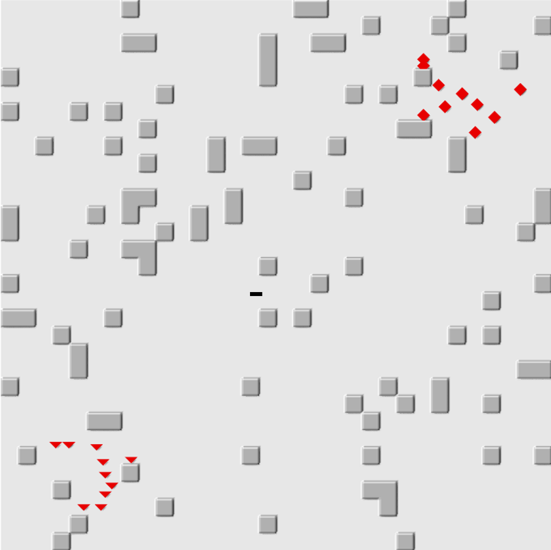
(g) 10 routes - CBS

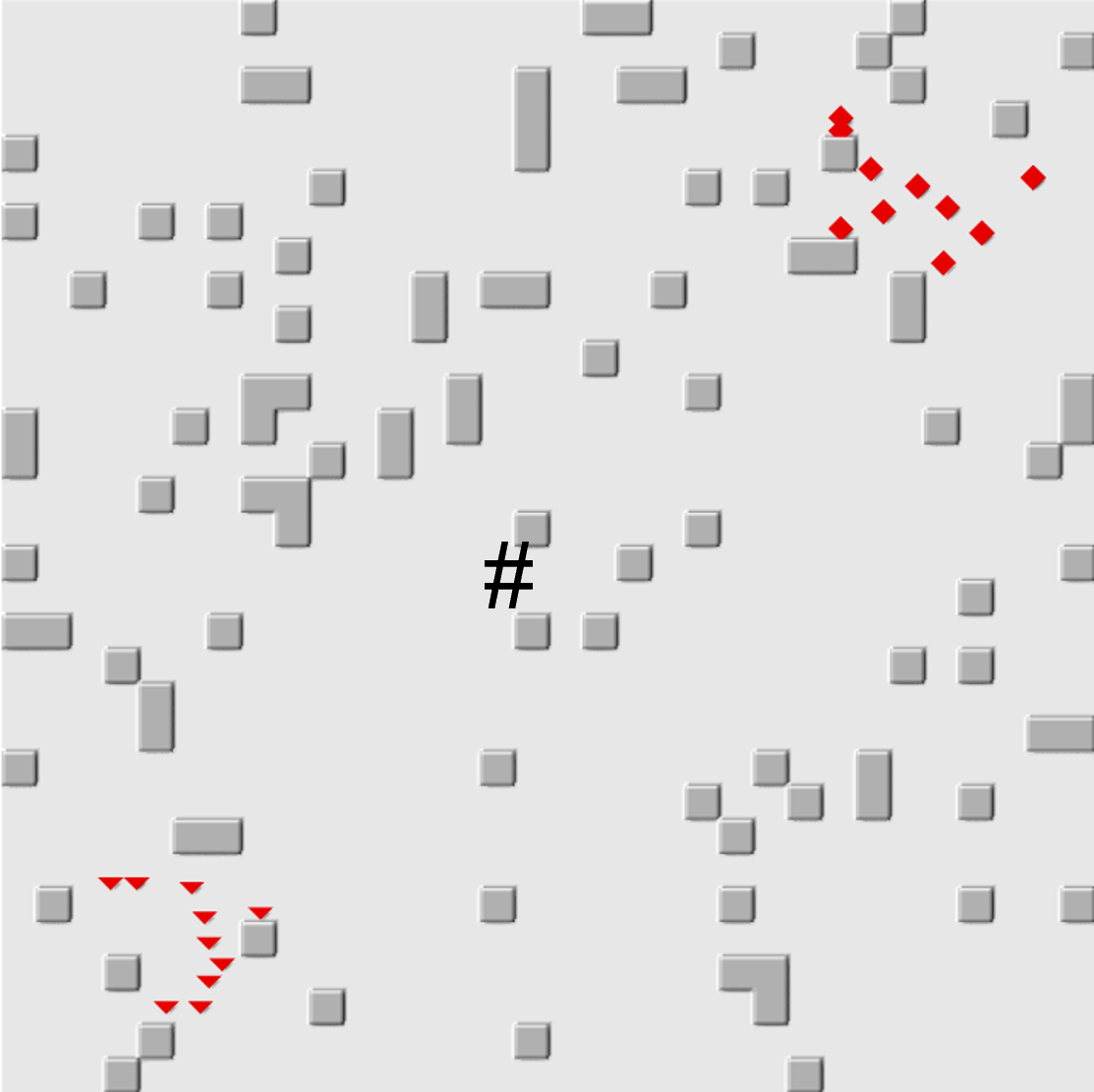
(h) 10 routes - Push-and-Spin

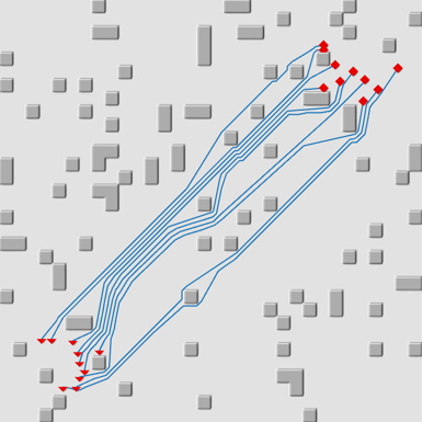
(i) 10 routes - The proposed method

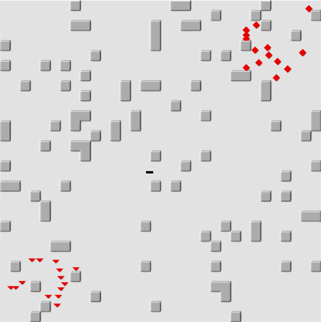
(j) 15 routes - CBS

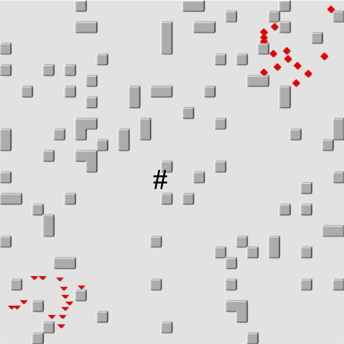
(k) 15 routes - Push-and-Spin

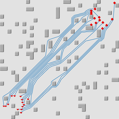
(l) 15 routes - The proposed method

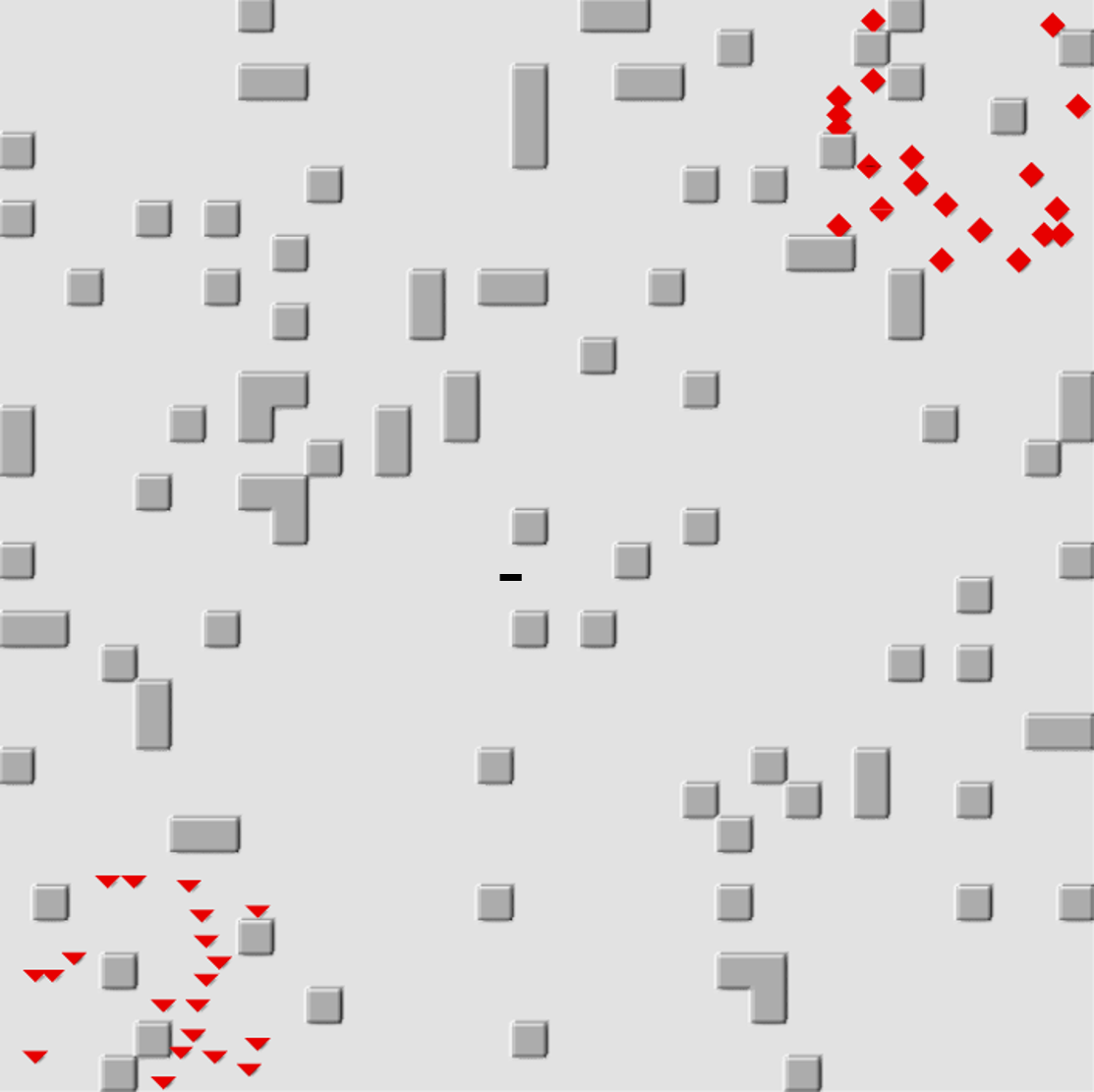
(m) 20 routes - CBS

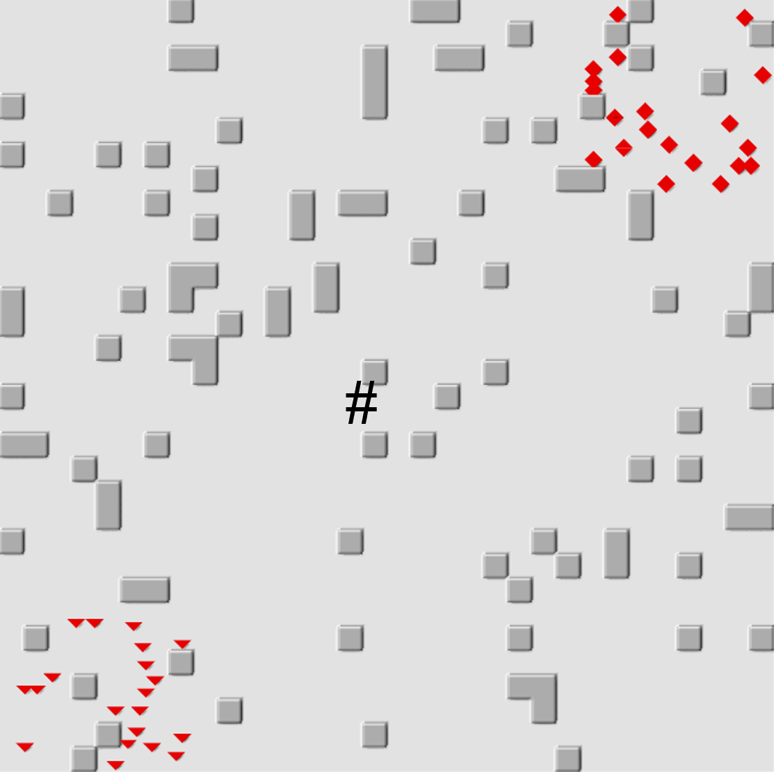
(n) 20 routes - Push-and-Spin

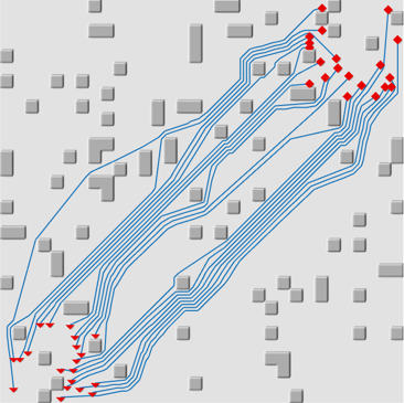
(o) 20 routes - The proposed method

Figure 15: Routes planned by CBS, Push-and-Spin, and the proposed method in the 2D standard test scenario

5.3 Demonstration on a Real-World Scenario

In this section, we use a real-world scenario to demonstrate the capabilty of the proposed method. The selected environment is a typical urban area in Hangzhou, China. Hangzhou has 10,711,198 residents (CITYPOPULATION, 2020) with a size of $8,292.31km^{2}$ for urban districts. Hangzhou has logged more than 3 billion express parcels (HangzhouPostal, 2020) in 2020. Drone delivery services have been offered by Antwork Technology in Hangzhou since 2020. The size of the selected area is $5.35km\times 2.95km$ (about $15.75km^{2}$) and the details of the scenario data are shown in Table 6. Drones are allowed to fly in the altitude range $[60m,120m]$. A graph is extracted from the scenario data using grid size $(10m,10m,10m)$. The details of the graph are shown in Table 7. In the flyable altitude range, there is a total of $946950$ cells and $707128$ cells are traversable.

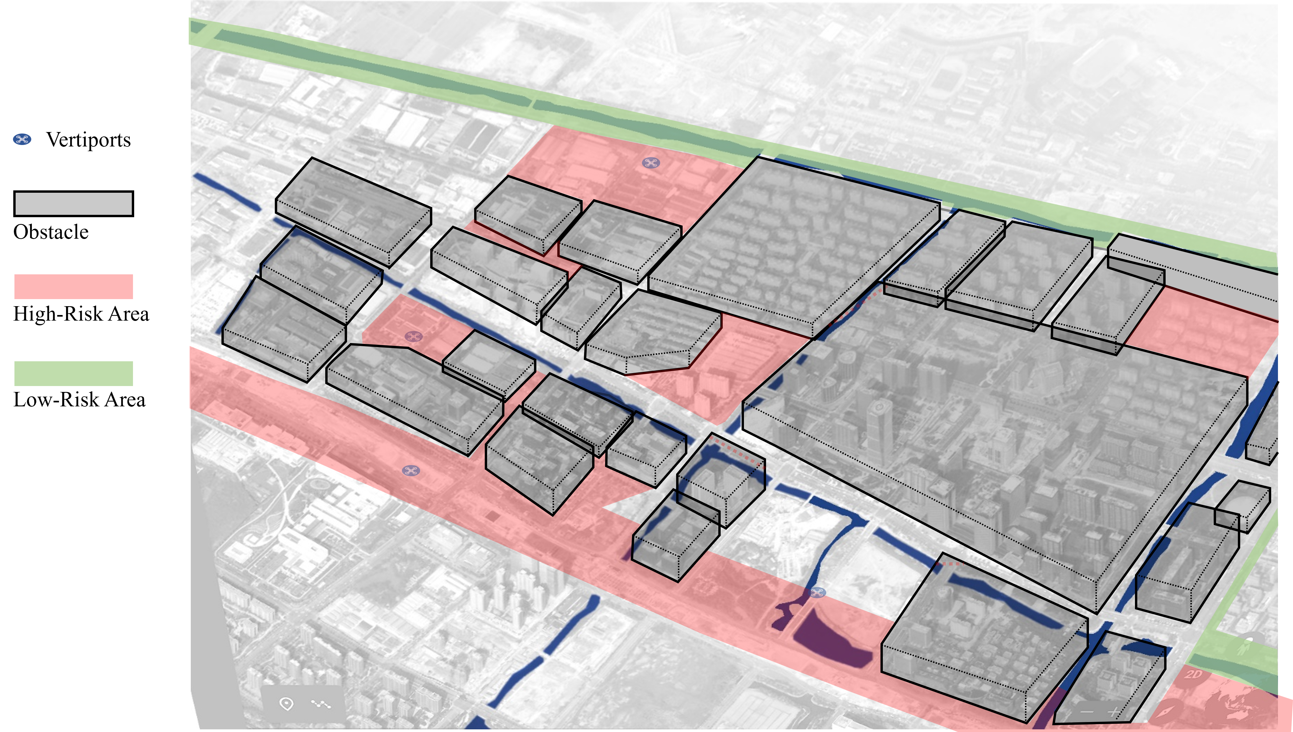
Figure 16: A real-world scenario in Hangzhou, China

In this urban area, 12 routes are planned using our proposed algorithm with the following parameter settings: $\varepsilon_{v}=1000,\omega_{r}=\omega_{p}=1.0$. The planned route network is shown in Figure 17, where paths are colored in blue. A few routes are aligned together with overlapped buffer zones, showing improved airspace utilization. Many paths are over green areas, which are preferred areas for drone operations with low risk. Only a few paths are over red areas, which have high risk, as the paths over normal regions are blocked by buildings. With an separate validity check, we confirm that the route network generated by the proposed method satisfies all operational constraints and can be used for drone delivery services.

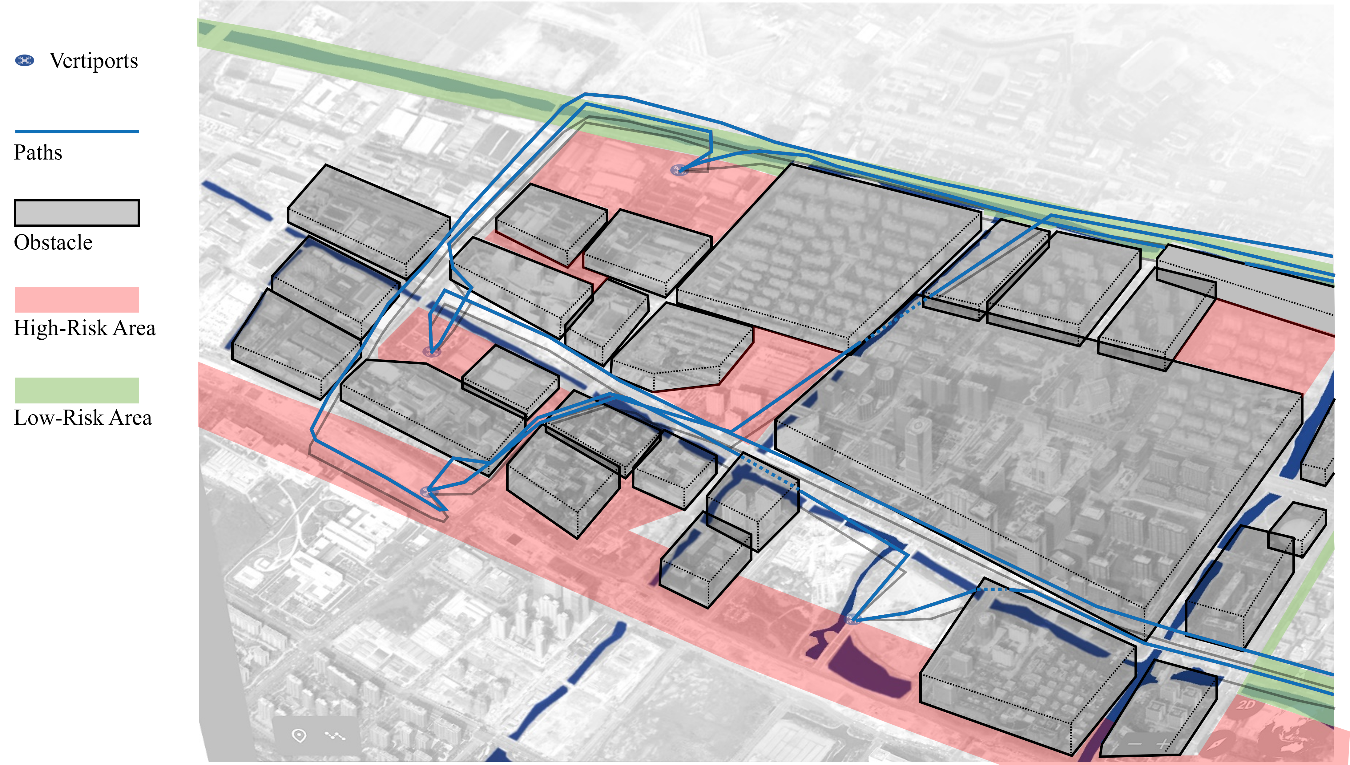
(a) Perspective view of all planned paths

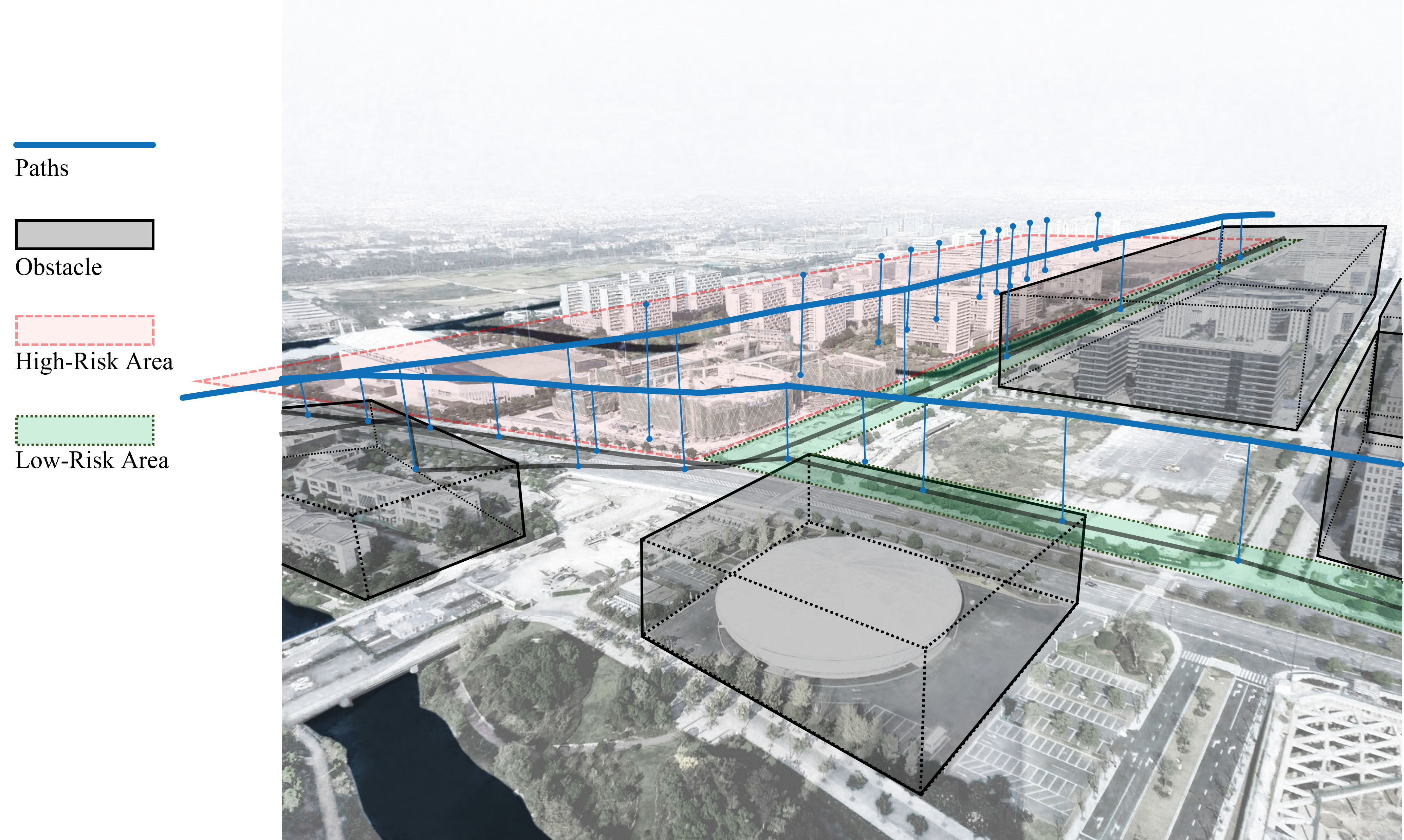
(b) A zoom-in view of the planned paths in relation to obstacles, high risk areas, and low risk areas

Figure 17: A set of paths planned by the proposed method (3D)

5.4 Sensitivity Analysis of Algorithm Parameters

5.4.1 Sensitivity Analysis on Space Cost

In this section, we analyze the effectiveness of adding the space cost into the algorithm by testing different values of the space cost weight coefficient $\omega_{p}$ in solving the network planning problem in the real-world 3D scenario in Section 5.3.

We first compare the routes found without space cost and the ones found with space cost. The results are shown in Table 3. Compared to routes found without space cost, the number of buffer zone cells decreased from 17.26 ‰ to 13.87 ‰, and the number of total occupied cells reduced from 24.14 ‰ to 21.51 ‰. Therefore, the proposed method with space cost can generate a route network that utilizes airspace more effectively than without space cost.

Table 3: Airspace occupancy for routes found without space cost vs. with space cost ^#

	buffer zone cells	Path cells	Total occupied cells
Without space cost ($\omega_{p}=0$)	17.26 ‰	6.88 ‰	24.14 ‰
Add space cost item ($\omega_{p}=1.0$)	13.87 ‰	6.89 ‰	21.51 ‰

• results are presented as the number of cells divides the total number of cells available for drones (707128)

Then we test how $\omega_{p}$ affects the planning of a route network. The results are shown in Figure 18. As $\omega_{p}$ increases, the number of buffer zone cells and the number of total occupied cells decrease; meanwhile, the number of path cells increases slightly, and the total cost of risk increases gradually as the relative weight on risks reduces compared to weight on airspace occupancy, resulting some routes fly over high risk areas to reduce space cost. Therefore, the relative value of the space cost coefficient in relation to other cost coefficients should be carefully calibrated so that the safety aspect is not compromised.

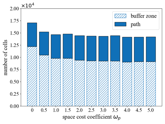
(a) Total occupied airspace (buffer zone vs. path)

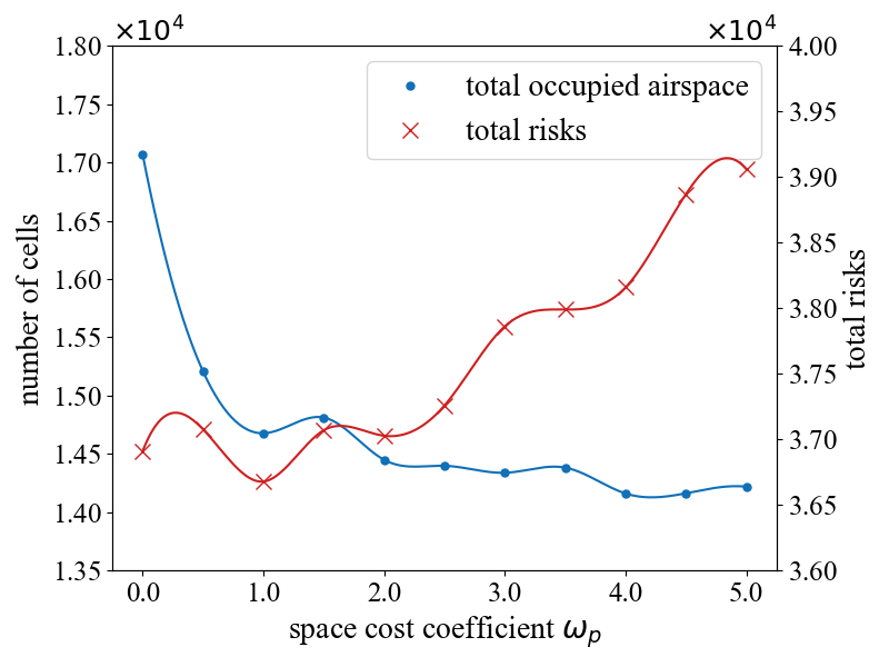
(b) Total occupied airspace vs. total risks

Figure 18: Sensitivity analysis on space cost coefficient $\omega_{p}$

5.4.2 Sensitivity Analysis on Route Prioritization Threshold

In this section, we first test the route network planning method with and without Route Prioritization module. Then we analyze how different values of the Route Prioritization threshold affect the results.

The result of comparison between no route prioritization and with route prioritization is shown in Table 4. With route prioritization, routes in Urgent and Important levels have smaller costs, but routes in Normal and Low levels have larger costs. The increase in normal and low levels is expected because route prioritization improves the quality of high-priority routes at the cost of low-priority routes. There is minimal impact on the total cost of the entire network from using route prioritization.

Table 4: Comparison between no route prioritization and with route prioritization

Average total cost after running 10 times#	Urgent	Important	Normal	Low	Total
No Route Prioritization	16030	4270	5572	11429	37301
With Route Prioritization*	15198	4091	6091	12331	37711
Improvement after route prioritization	832	179	-519	-901	-410

• Sequences without prioritization vary, the average cost is used.

• Thresholds $\varepsilon_{v}=1000$, the range of profit $v$ is $[-219,9765]$.

For the sensitivity analysis on threshold values, we take $\varepsilon_{v}$ as an example to show how threshold values affect the route prioritization and the final result. Here we use 16 OD pairs, and the potential profit values of these OD pairs are derived from a normal distribution $v\sim\mathcal{N}(5000,2000)$. We test the threshold values $\varepsilon_{v}\in\{100,400,800\}$. As shown by the results in Table 5, with the increase of $\varepsilon_{v}$, OD pairs are divided into fewer but larger subsequences, making the total number of possible ordered arrangements $S_{g}$ larger, and the minimum total costs for the networks decrease. This is because with more permutation of OD sequences being tested, the results solution gets closer to the optimal one. However, it is at the cost of increased computational time.

Table 5: Sensitivity Analysis on Threshold of Expected Profit Values $\varepsilon_{v}$

OD pairs sorted by expected profit values $v$
route $i$	$r_{1}$	$r_{2}$	$r_{3}$	$r_{4}$	$r_{5}$	$r_{6}$	$r_{7}$	$r_{8}$
$v$	$9481$	$8735$	$7988$	$7908$	$6957$	$6900$	$6522$	$5821$
route $i$	$r_{9}$	$r_{10}$	$r_{11}$	$r_{12}$	$r_{13}$	$r_{14}$	$r_{15}$	$r_{16}$
$v$	$5800$	$5667$	$5626$	$5423$	$4793$	$4697$	$3045$	$-105$
$\mathbf{\varepsilon_{v}=100}$
Best total costs: 35098			Shuffled times: $K=10$			Total randomness: $S_{g}=32$
subsequences: $[(r_{1}),(r_{2}),(r_{3},r_{4}),(r_{5},r_{6}),(r_{7}),(r_{8},r_{9}),(r_{10},r_{11}),(r_{12}),(r_{13},r_{14}),(r_{15}),(r_{16})]$
$\mathbf{\varepsilon_{v}=400}$
Best total costs: 33810			Shuffled times: $K=100$			Total randomness: $S_{g}=960$
subsequences: $[(r_{1}),(r_{2}),(r_{3},r_{4}),(r_{5},r_{6}),(r_{7}),(r_{8},r_{9},r_{10},r_{11},r_{12}),(r_{13},r_{14}),(r_{15}),(r_{16})]$
$\mathbf{\varepsilon_{v}=800}$
Best total costs: 33659			Shuffled times: $K=200$			Total randomness: $S_{g}=1440$
subsequences: $[(r_{1},r_{2}),(r_{3},r_{4}),(r_{5},r_{6},r_{7}),(r_{8},r_{9},r_{10},r_{11},r_{12}),(r_{13},r_{14}),(r_{15}),(r_{16})]$

5.5 Algorithm Scalability and Computational Time

In this section, we first show how the computational time of the algorithm is affected by the random shuffle times $K$, and then we show how the computational time of the algorithm increases as the number of routes increases. The test scenario is the urban area in Hangzhou as shown in Section 5.3. All experiments are performed on a platform Intel(R) Xeon(R) Gold 5218 CPU @ 2.30GHz.

The computational times for different $K$ are shown in Figure 19. As $K$ increases, the computational time increases proportionally. This means that the total computational time is proportional to the number of OD pair sequences to run. The computational times for different number of routes to plan are shown in Figure 20 and the result data are summarized in table 8 in the Appendix. When $K$ is fixed, with the increase of the number of routes $N$, the computational time increases near linearly. The empirical results show that the proposed method is able to handle the planning of 40 routes within about 1 hour for a real-world scenario.

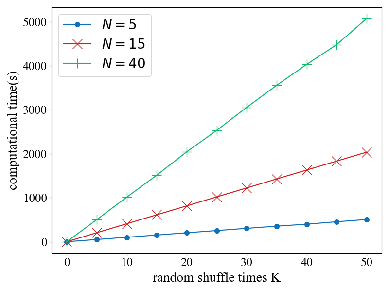
Figure 19: Sensitivity analysis on random shuffle times $K$ for different number of routes $N$

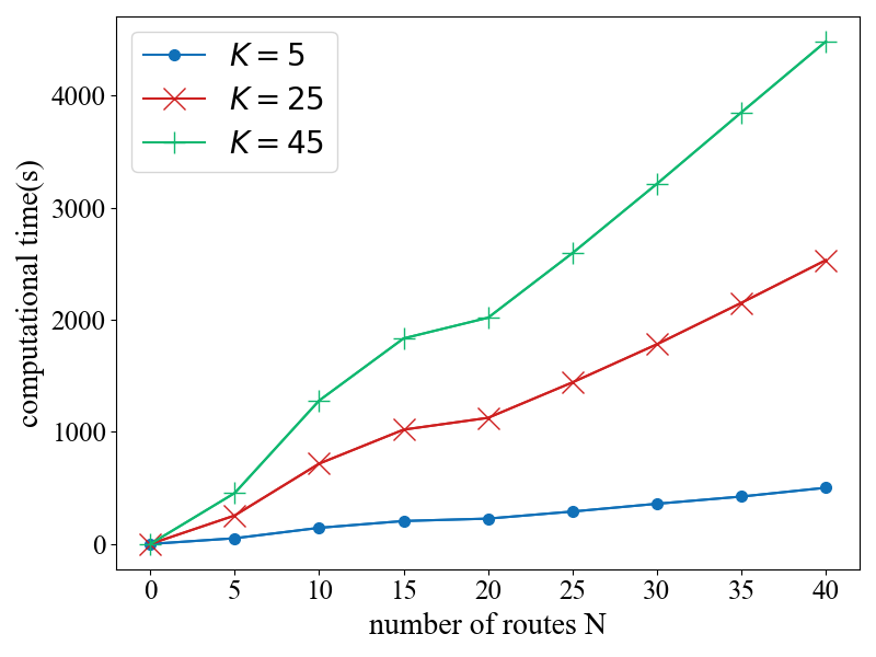
Figure 20: Algorithm scalability as the number of routes increases

Antwork Technology’s current drone delivery network operates up to 80-100 flights per day on 50 unidirectional air routes. The length of the air routes is about 10 km on average, and the longest one is more than 30 km. These air routes are manually designed at Antwork Technology. To design a route, a field study needs to be conducted first to obtain 3D modelling of the environment. Based on the detailed 3D model, an air route is manually charted and then checked to see whether it satisfies all operational requirements. It usually takes 2 to 4 hours to design one air route. Moreover, it becomes infeasible to design a network with a large number of air routes once the complexity exceeds human operators’ capability.

The proposed method is expected to significantly improve the design process of the air route network by making it automatic. With the proposed method, the design of a network with 40 air routes within 1 hour. Also, the scale of the network will no longer be limited by human operators’ capability of dealing with the computational complexity. Using the proposed method, more routes can be designed until the airspace cannot accommodate any additional air routes.

6 Conclusion

This paper proposed a sequential route network planning method to support tube-based operations of drone deliveries. The proposed method is capable of designing a spatially separated tube-based route network in a large urban area within a reasonable time. The method is composed of four modules: Environment Discretization, Individual Route Planning, Route Prioritization, and Network Planning. The proposed prioritization structure decoupled the network planning problem into a sequential single-path-planning problem. The space cost function in the Individual Route Planning module made it possible to have the routes aligned and grouped together. A set of tests were carried out to show our method can generate route networks that satisfy all requirements within a short time and can be taken for commercial use. With the implementation of the proposed method, drone delivery service providers can quickly design a drone route network, and re-plan on a daily basis to respond to changes in their service network. With the route prioritization function, they can prioritize the design of urgent or important deliveries. The space cost function allowed higher airspace utilization and potentially led to the identification of high-volume air corridors in an urban area. From the city residents’ perspective, less areas would be affected by this new type of aerial operations.

One direction of future work is to further reduce computational time while ensuring the optimality of the solution and the fairness between different routes. Distributed planning is a promising direction to explore.

Another direction to adapt the method to build tube-based route networks for other applications, where many moving agents should be transported among OD pairs. In the tube-based route network, one or multiple tubes can be planned to connect an OD pair based on the traveling demand. The moving agents following a tube can sequentially pass to arrive at the destination. Besides the drone route network, an example situation is warehouse logistics. In such a situation, robots should move packages from one place to another place, and the proposed method can be applied to plan the paths for these robots.

Appendix A: Calculation for $\lambda_{r}$ and $\lambda_{p}$

$\lambda_{r}$ is calculated as $\lambda_{r}=\frac{o_{0}(s_{start},s_{goal})}{r_{0}(s_{start},s_{goal})}$, where $o_{0}(s_{start},s_{goal})$ is the minimum operational cost and $r_{0}(s_{start},s_{goal})$ is the minimum risk cost for a conflict-free path that connects $s_{start}$ and $s_{goal}$.

$\lambda_{p}$ is calculated as $\lambda_{p}=\frac{o_{0}(s_{start},s_{goal})}{p_{0}(s_{start},s_{goal})}$, where $o_{0}(s_{start},s_{goal})$ is the minimum operational cost and $p_{0}(s_{start},s_{goal})$ is the minimum space cost for a conflict-free path that connects $s_{start}$ and $s_{goal}$.

Appendix B: Real-World Scenario Data Specifications

Table 6: Description for real-world scenario data

Types	Number	Attributes
Vertiports	7	Id, type, radius, {latitude, longitude, altitude}
Obstacles	55	Id, highest / lowest altitude, points (latitudes, longitudes)
High / low risk area	22	Id, risk level, points (latitudes, longitudes)

Table 7: Summary for real-world scenario

Name	Value	Example
Bounding box	X-direction	$[-1780.99m,3566.63m]$
	Y-direction	$[-1177.21m,1768.74m]$
	Z-direction	$[0m,260m]$
Traversable layer	Z-direction	$[60m,120m]$
Map size	Total area	$15.75km^{2}$
	Grid size	$(10m,10m,10m)$
	Number of grids	$535*295*6=946950$
	Number of traversable grids	$707128(74.7\%)$
Cell attributes	Risk	$(0,1)\to$ low risk area
		$(1,\infty)\to$ high risk area
		$1\to$ normal area
	Reachable	True or False
	Reserved	True or False
	Buffer	True or False

Appendix C: Computational time for different Random shuffle Times $K$ and number of routes $N$

Table 8: Computational time (s) for different Random shuffle Times $K$ and number of routes $N$

	0	5	10	15	20	25	30	35	40	45	50
0	0	0	0	0	0	0	0	0	0	0	0
5	0	51.0	102.0	153.1	204.2	254.3	304.6	354.1	399.0	454.6	505.5
10	0	144.1	286.3	426.5	579.5	716.7	858.1	996.3	1127.1	1279.3	1430.3
15	0	204.8	408.5	612.2	815.2	1019.7	1222.6	1427.8	1630.3	1833.6	2035.6
20	0	226.2	450.7	673.7	898.3	1124.9	1347.7	1570.4	1795.0	2017.8	2242.8
25	0	289.3	577.2	864.0	1152.6	1441.3	1729.8	2018.4	2307.0	2594.5	2885.1
30	0	358.6	712.0	1067.0	1426.0	1781.0	2139.2	2498.0	2854.6	3212.1	3567.2
35	0	422.8	847.6	1298.6	1726.8	2150.5	2578.8	3001.5	3426.0	3849.0	4272.7
40	0	501.5	1011.9	1512.5	2043.4	2531.1	3054.1	3556.6	4031.7	4480.7	5074.0

References

- Alotaibi & Al-Rawi (2018) Alotaibi, E. T. S., & Al-Rawi, H. (2018). A complete multi-robot path-planning algorithm. Autonomous Agents and Multi-Agent Systems, 32, 693–740. doi:10.1007/s10458-018-9391-2.
- Barer et al. (2014) Barer, M., Sharon, G., Stern, R., & Felner, A. (2014). Suboptimal variants of the conflict-based search algorithm for the multi-agent pathfinding problem. In Seventh Annual Symposium on Combinatorial Search.
- Bauranov & Rakas (2021) Bauranov, A., & Rakas, J. (2021). Designing airspace for urban air mobility: A review of concepts and approaches. Progress in Aerospace Sciences, 125, 100726. doi:10.1016/j.paerosci.2021.100726.
- Bertram et al. (2021) Bertram, J., Wei, P., & Zambreno, J. (2021). Scalable fastmdp for pre-departure airspace reservation and strategic de-conflict. In AIAA Scitech 2021 Forum (p. 0779).
- Bhattacharya et al. (2010) Bhattacharya, S., Kumar, V., & Likachev, M. (2010). Distributed optimization with pairwise constraints and its application to multi-robot path planning. In Robotics: Science and Systems VI (pp. 87–94). Robotics: Science and Systems Foundation volume 177. URL: http://www.roboticsproceedings.org/rss06/p23.pdf. doi:10.15607/RSS.2010.VI.023.
- Bin Mohammed Salleh et al. (2018) Bin Mohammed Salleh, M. F., Chi, W., Wang, Z., Huang, S., Tan, D. Y., Huang, T., & Low, K. H. (2018). Preliminary concept of adaptive urban airspace management for unmanned aircraft operations. In AIAA Information Systems-AIAA Infotech at Aerospace, January 8-12, 2018 (p. 2260). Kissimmee, Florida, USA. doi:10.2514/6.2018-2260.
- Bnaya & Felner (2014) Bnaya, Z., & Felner, A. (2014). Conflict-oriented windowed hierarchical cooperative a*. In 2014 IEEE International Conference on Robotics and Automation (ICRA) (pp. 3743–3748). IEEE.
- Cekmez et al. (2014) Cekmez, U., Ozsiginan, M., & Sahingoz, O. K. (2014). A uav path planning with parallel aco algorithm on cuda platform. In 2014 International Conference on Unmanned Aircraft Systems (ICUAS) (pp. 347–354). IEEE.
- Chamseddine et al. (2012) Chamseddine, A., Zhang, Y., Rabbath, C. A., Join, C., & Theilliol, D. (2012). Flatness-based trajectory planning/replanning for a quadrotor unmanned aerial vehicle. IEEE Transactions on Aerospace and Electronic Systems, 48, 2832–2847. doi:10.1109/TAES.2012.6324664.
- Chung (2021) Chung, S.-H. (2021). Applications of smart technologies in logistics and transport: A review. Transportation Research Part E: Logistics and Transportation Review, 153, 102455. doi:10.1016/j.tre.2021.102455.
- CITYPOPULATION (2020) CITYPOPULATION (2020). China: Zhejiang. URL: https://www.citypopulation.de/en/china/zhejiang/admin/.
- Cohen et al. (2019) Cohen, L., Uras, T., Kumar, T. S., & Koenig, S. (2019). Optimal and bounded-suboptimal multi-agent motion planning. In Twelfth Annual Symposium on Combinatorial Search.
- Cohen et al. (2016) Cohen, L., Uras, T., Kumar, T. S., Xu, H., Ayanian, N., & Koenig, S. (2016). Improved solvers for bounded-suboptimal multi-agent path finding. In IJCAI (pp. 3067–3074).
- Culligan et al. (2007) Culligan, K., Valenti, M., Kuwata, Y., & How, J. P. (2007). Three-dimensional flight experiments using on-line mixed-integer linear programming trajectory optimization. In Proceedings of the American Control Conference, July 11-13, 2007 (pp. 5322–5327). New York, NY, USA. doi:10.1109/ACC.2007.4283101.
- Daniel et al. (2010) Daniel, K., Nash, A., Koenig, S., & Felner, A. (2010). Theta*: Any-angle path planning on grids. Journal of Artificial Intelligence Research, 39, 533–579. URL: https://www.jair.org/index.php/jair/article/view/10676. doi:10.1613/jair.2994.
- De Wilde et al. (2014) De Wilde, B., Ter Mors, A. W., & Witteveen, C. (2014). Push and rotate: a complete multi-agent pathfinding algorithm. Journal of Artificial Intelligence Research, 51, 443–492. doi:10.1613/jair.4447.
- Dezfoulian et al. (2013) Dezfoulian, S. H., Wu, D., & Ahmad, I. S. (2013). A generalized neural network approach to mobile robot navigation and obstacle avoidance. In Intelligent autonomous systems 12 (pp. 25–42). Springer.
- Dijkstra (1959) Dijkstra, E. W. (1959). A note on two problems in connexion with graphs. Numerische Mathematik, 1, 269–271. doi:10.1007/BF01386390.
- Duvall et al. (2019) Duvall, T., Green, A., Langstaff, M., & Miele, K. (2019). Air-mobility solutions: What they’ll need to take off. URL: www.mckinsey.com/industries/capital-projects-and-infrastructure/our-insights/air-mobility-solutions-what-theyll-need-to-take-off.
- Englot & Hover (2011) Englot, B., & Hover, F. (2011). Multi-goal feasible path planning using ant colony optimization. In 2011 IEEE International Conference on Robotics and Automation (pp. 2255–2260). IEEE.
- Ester et al. (1996) Ester, M., Kriegel, H.-P., Sander, J., & Xu, X. (1996). A density-based algorithm for discovering clusters in large spatial databases with noise. In Proceedings of the 2nd International Conference on Knowledge Discovery and Data Mining, August 2-4, 1996 (pp. 226–231). volume 96.
- EUROCONTROL (2018) EUROCONTROL (2018). Unmanned Aircraft Systems (UAS) ATM Integration. URL: https://www.eurocontrol.int/publication/unmanned-aircraft-systems-uas-atm-integration.
- Felner et al. (2012) Felner, A., Goldenberg, M., Sharon, G., Stern, R., Beja, T., Sturtevant, N. R., Schaeffer, J., & Holte, R. (2012). Partial-Expansion A* with Selective Node Generation. In Proceedings of the Twenty-Sixth AAAI Conference on Artificial Intelligence, July 22-26, 2012 (pp. 471–477). Toronto, Ontario, Canada: Toronto, Ontario.
- Felner et al. (2017) Felner, A., Stern, R., Shimony, S. E., Boyarski, E., Goldenberg, M., Sharon, G., Sturtevant, N., Wagner, G., & Surynek, P. (2017). Search-based optimal solvers for the multi-agent pathfinding problem: Summary and challenges. Proceedings of the 10th Annual Symposium on Combinatorial Search, SoCS 2017, 2017-Janua, 29–37.
- Gilboa et al. (2006) Gilboa, A., Meisels, A., & Felner, A. (2006). Distributed navigation in an unknown physical environment. In Proceedings of the fifth international joint conference on Autonomous agents and multiagent systems (pp. 553–560). New York, New York, USA: ACM Press. doi:10.1145/1160633.1160735.
- Goldenberg et al. (2014) Goldenberg, M., Felner, A., Stern, R., Sharon, G., Sturtevant, N., Holte, R. C., & Schaeffer, J. (2014). Enhanced partial expansion A. Journal of Artificial Intelligence Research, 50, 141–187. doi:10.1613/jair.4171.
- Grady et al. (2010) Grady, D. K., Bekris, K. E., & Kavraki, L. E. (2010). Asynchronous distributed motion planning with safety guarantees under second-order dynamics. In Algorithmic foundations of robotics IX (pp. 53–70). Springer, Berlin, Heidelberg volume 68. doi:10.1007/978-3-642-17452-0_4.
- Ha et al. (2018) Ha, Q. M., Deville, Y., Pham, Q. D., & Hà, M. H. (2018). On the min-cost traveling salesman problem with drone. Transportation Research Part C: Emerging Technologies, 86, 597–621. doi:10.1016/j.trc.2017.11.015. arXiv:1512.01503.
- HangzhouPostal (2020) HangzhouPostal (2020). Hangzhou express logistics industry develops steadily in 2020. URL: https://www.hangzhou.gov.cn/art/2020/12/31/art_812262_59023763.html.
- Hart et al. (1968) Hart, P. E., Nilsson, N. J., & Raphael, B. (1968). A formal basis for the heuristic determination of minimum cost paths. IEEE Transactions on Systems Science and Cybernetics, 4, 100--107. doi:10.1109/TSSC.1968.300136.
- Hoekstra et al. (2018) Hoekstra, J. M., Ellerbroek, J., Sunil, E., & Maas, J. (2018). Geovectoring: reducing traffic complexity to increase the capacity of uav airspace. In International Conference for Research in Air Transportation, Barcelona, Spain.
- Hoekstra et al. (2002) Hoekstra, J. M., Van Gent, R. N., & Ruigrok, R. C. (2002). Designing for safety: The ’free flight’ air traffic management concept. Reliability Engineering and System Safety, 75, 215--232. doi:10.1016/S0951-8320(01)00096-5.
- Hu & Yang (2004) Hu, Y., & Yang, S. X. (2004). A knowledge based genetic algorithm for path planning of a mobile robot. In IEEE International Conference on Robotics and Automation (pp. 4350--4355). IEEE volume 5.
- Islami et al. (2017) Islami, A., Chaimatanan, S., & Delahaye, D. (2017). Large-scale 4d trajectory planning. In Air Traffic Management and Systems II (pp. 27--47). Springer.
- Jang et al. (2017) Jang, D. S., Ippolito, C., Sankararaman, S., & Stepanyan, V. (2017). Concepts of airspace structures and system analysis for uas traffic flows for urban areas. In AIAA Information Systems-AIAA Infotech at Aerospace, January 9-13, 2017 (p. 0449). Grapevine, Texas, USA. doi:10.2514/6.2017-0449.
- Jardin (2005) Jardin, M. R. (2005). Analytical relationships between conflict counts and air-traffic density. Journal of guidance, control, and dynamics, 28, 1150--1156. doi:10.2514/1.12758.
- Kant & Zucker (1986) Kant, K., & Zucker, S. W. (1986). Toward efficient trajectory planning: The path-velocity decomposition. The international journal of robotics research, 5, 72--89. doi:10.1177/027836498600500304.
- Karak & Abdelghany (2019) Karak, A., & Abdelghany, K. (2019). The hybrid vehicle-drone routing problem for pick-up and delivery services. Transportation Research Part C: Emerging Technologies, 102, 427--449. doi:10.1016/j.trc.2019.03.021.
- Karaman & Frazzoli (2011) Karaman, S., & Frazzoli, E. (2011). Sampling-based algorithms for optimal motion planning. The international journal of robotics research, 30, 846--894.
- Kavraki et al. (1996) Kavraki, L. E., Švestka, P., Latombe, J. C., & Overmars, M. H. (1996). Probabilistic roadmaps for path planning in high-dimensional configuration spaces. IEEE Transactions on Robotics and Automation, 12, 566--580. doi:10.1109/70.508439.
- Kellermann et al. (2020) Kellermann, R., Biehle, T., & Fischer, L. (2020). Drones for parcel and passenger transportation: A literature review. Transportation Research Interdisciplinary Perspectives, 4, 100088.
- Kersten et al. (2021) Kersten, H., Benedikt, K., & Robin, R. (2021). Advanced air mobility in 2030. URL: https://www.mckinsey.com/industries/aerospace-and-defense/our-insights/advanced-air-mobility-in-2030.
- Kitonsa & Kruglikov (2018) Kitonsa, H., & Kruglikov, S. V. (2018). Significance of drone technology for achievement of the united nations sustainable development goals. R-economy, 4, 115--120.
- Koenig & Likhachev (2005) Koenig, S., & Likhachev, M. (2005). Fast replanning for navigation in unknown terrain. IEEE Transactions on Robotics, 21, 354--363. doi:10.1109/TRO.2004.838026.
- Kopardekar (2014) Kopardekar, P. (2014). Unmanned Aerial System (UAS) Traffic Management (UTM): Enabling Low-Altitude Airspace and UAS Operations. URL: https://ntrs.nasa.gov/api/citations/20140013436/downloads/20140013436.pdf.
- Kopardekar et al. (2016) Kopardekar, P., Rios, J., Prevot, T., Johnson, M., Jung, J., & Robinson, J. E. (2016). Unmanned aircraft system traffic management (utm) concept of operations. In 16th AIAA Aviation Technology, Integration, and Operations Conference, June 13-17, 2016 (pp. 1--16). Washington, D.C., USA. doi:10.2514/6.2016-3292.
- Kornhauser et al. (1984) Kornhauser, D., Miller, G., & Spirakis, P. (1984). Coordinating pebble motion on graphs, the diameter of permutation groups, and applications. In 25th Annual Symposium on Foundations of Computer Science, 1984. (pp. 241--250). IEEE.
- Krozel et al. (2001) Krozel, J., Peters, M., Bilimoria, K. D., Lee, C., & Mitchell, J. S. (2001). System performance characteristics of centralized and decentralized air traffic separation strategies. Air Traffic Control Quarterly, 9, 311--332. doi:10.2514/atcq.9.4.311.
- Kuchar & Yang (2000) Kuchar, J. K., & Yang, L. C. (2000). A review of conflict detection and resolution modeling methods. IEEE Transactions on intelligent transportation systems, 1, 179--189.
- Lavalle (1998) Lavalle, S. M. (1998). Rapidly-exploring random trees: A new tool for path planning. Technical report, Iowa State University,, . URL: http://citeseerx.ist.psu.edu/viewdoc/summary?doi=10.1.1.35.1853.
- Lemardelé et al. (2021) Lemardelé, C., Estrada, M., Pagès, L., & Bachofner, M. (2021). Potentialities of drones and ground autonomous delivery devices for last-mile logistics. Transportation Research Part E: Logistics and Transportation Review, 149, 102325. doi:10.1016/j.tre.2021.102325.
- Leroy et al. (1999) Leroy, S., Laumond, J.-P., & Siméon, T. (1999). Multiple path coordination for mobile robots: A geometric algorithm. In Proceedings of the Sixteenth International Joint Conference on Artificial Intelligence (IJCAI), July 31-August 6, 1999 (pp. 1118--1123). Stockholm, Sweden volume 2.
- Li et al. (2005) Li, Y., Gupta, K., & Payandeh, S. (2005). Motion planning of multiple agents in virtual environments using coordination graphs. In Proceedings of the 2005 IEEE International Conference on Robotics and Automation, April 18-22, 2005 (pp. 378--383). Barcelona, Spain, Spain: IEEE. doi:10.1109/ROBOT.2005.1570148.
- Liu et al. (2020) Liu, S., Jiang, H., Chen, S., Ye, J., He, R., & Sun, Z. (2020). Integrating dijkstra’s algorithm into deep inverse reinforcement learning for food delivery route planning. Transportation Research Part E: Logistics and Transportation Review, 142, 102070. doi:10.1016/j.tre.2020.102070.
- Luna & Bekris (2011) Luna, R., & Bekris, K. E. (2011). Efficient and complete centralized multi-robot path planning. In 2011 IEEE/RSJ International Conference on Intelligent Robots and Systems, September 25-30, 2011 (pp. 3268--3275). San Francisco, CA, USA: IEEE. doi:10.1109/IROS.2011.6095085.
- Masehian & Sedighizadeh (2010) Masehian, E., & Sedighizadeh, D. (2010). Multi-objective pso-and npso-based algorithms for robot path planning. Advances in electrical and computer engineering, 10, 69--76.
- Mohamed Salleh et al. (2018) Mohamed Salleh, M. F. B., Wanchao, C., Wang, Z., Huang, S., Tan, D. Y., Huang, T., & Low, K. H. (2018). Preliminary concept of adaptive urban airspace management for unmanned aircraft operations. In 2018 AIAA Information Systems-AIAA Infotech@ Aerospace (p. 2260).
- MorganStanley (2021) MorganStanley (2021). evtol/urban air mobility tam update: A slow take-off, but sky’s the limit. URL: https://assets.verticalmag.com/wp-content/uploads/2021/05/Morgan-Stanley-URBAN_20210506_0000.pdf.
- Moshref-Javadi et al. (2020) Moshref-Javadi, M., Lee, S., & Winkenbach, M. (2020). Design and evaluation of a multi-trip delivery model with truck and drones. Transportation Research Part E: Logistics and Transportation Review, 136, 101887. doi:10.1016/j.tre.2020.101887.
- Murray & Chu (2015) Murray, C. C., & Chu, A. G. (2015). The flying sidekick traveling salesman problem: Optimization of drone-assisted parcel delivery. Transportation Research Part C: Emerging Technologies, 54, 86--109. doi:10.1016/j.trc.2015.03.005.
- Murray & Raj (2020) Murray, C. C., & Raj, R. (2020). The multiple flying sidekicks traveling salesman problem: Parcel delivery with multiple drones. Transportation Research Part C: Emerging Technologies, 110, 368--398. doi:10.1016/j.trc.2019.11.003.
- NASA (2021) NASA (2021). Utm concept of operations v2.0. URL: https://www.faa.gov/uas/research_development/traffic_management/media/UTM_ConOps_v2.pdf.
- Octavian Thor & Bogdan (2009) Octavian Thor, P., & Bogdan, D. (2009). Free flight vs. centralized air traffic management. Incas Bulletin, 3, 67--75. doi:10.13111/2066-8201.2011.3.4.7.
- O’Donnell & Lozano-Pérez (1989) O’Donnell, P. A., & Lozano-Pérez, T. (1989). Deadlock-free and collision-free coordination of two robot manipulators. In 1989 International Conference on Robotics and Automation (ICRA), May 14-19, 1989 (pp. 484--489). Scottsdale, AZ, USA: IEEE. doi:10.1109/ROBOT.1989.100033.
- Peng & Akella (2005) Peng, J., & Akella, S. (2005). Coordinating multiple robots with kinodynamic constraints along specified paths. The International Journal of Robotics Research, 24, 295--310. doi:10.1177/0278364905051974.
- Rajendran & Srinivas (2020) Rajendran, S., & Srinivas, S. (2020). Air taxi service for urban mobility: a critical review of recent developments, future challenges, and opportunities. Transportation research part E: logistics and transportation review, 143, 102090. doi:10.1016/j.tre.2020.102090.
- Ryan (2010) Ryan, M. (2010). Constraint-based multi-robot path planning. In 2010 IEEE International Conference on Robotics and Automation, May 4 - 8, 2010 (pp. 922--928). Anchorage, Alaska, USA: IEEE. doi:10.1109/ROBOT.2010.5509582.
- Sacramento et al. (2019) Sacramento, D., Pisinger, D., & Ropke, S. (2019). An adaptive large neighborhood search metaheuristic for the vehicle routing problem with drones. Transportation Research Part C: Emerging Technologies, 102, 289--315. doi:10.1016/j.trc.2019.02.018.
- Saha & Isto (2006) Saha, M., & Isto, P. (2006). Multi-robot motion planning by incremental coordination. In 2006 IEEE/RSJ International Conference on Intelligent Robots and Systems, October 9-15, 2006 (pp. 5960--5963). Beijing, China: IEEE. doi:10.1109/IROS.2006.282536.
- Sanchez & Latombe (2002) Sanchez, G., & Latombe, J.-C. (2002). Using a prm planner to compare centralized and decoupled planning for multi-robot systems. In Proceedings 2002 IEEE International Conference on Robotics and Automation (Cat. No.02CH37292), May 11-15, 2002 (pp. 2112--2119). Washington, DC, USA: IEEE volume 2. doi:10.1109/ROBOT.2002.1014852.
- Schermer et al. (2019) Schermer, D., Moeini, M., & Wendt, O. (2019). A matheuristic for the vehicle routing problem with drones and its variants. Transportation Research Part C: Emerging Technologies, 106, 166--204. doi:10.1016/j.trc.2019.06.016.
- SESAR (2019) SESAR (2019). Sesar concept of operations for u-space. URL: https://www.sesarju.eu/node/3411.
- Sharon et al. (2015) Sharon, G., Stern, R., Felner, A., & Sturtevant, N. R. (2015). Conflict-based search for optimal multi-agent pathfinding. Artificial Intelligence, 219, 40--66. doi:10.1016/j.artint.2014.11.006.
- Sharon et al. (2013) Sharon, G., Stern, R., Goldenberg, M., & Felner, A. (2013). The increasing cost tree search for optimal multi-agent pathfinding. Artificial Intelligence, 195, 470--495. doi:10.1016/j.artint.2012.11.006.
- Shen et al. (2020) Shen, L., Wang, Y., Liu, K., Yang, Z., Shi, X., Yang, X., & Jing, K. (2020). Synergistic path planning of multi-uavs for air pollution detection of ships in ports. Transportation Research Part E: Logistics and Transportation Review, 144, 102128. doi:10.1016/j.tre.2020.102128.
- Silver (2005) Silver, D. (2005). Cooperative pathfinding. In Proceedings of the First Artificial Intelligence and Interactive Digital Entertainment, June 1-5, 2005 (pp. 117--122). Marina del Rey, California, USA: Marina Del Rey volume 1.
- Singh & Thongam (2019) Singh, N. H., & Thongam, K. (2019). Neural network-based approaches for mobile robot navigation in static and moving obstacles environments. Intelligent Service Robotics, 12, 55--67.
- Škrinjar et al. (2019) Škrinjar, J. P., Škorput, P., & Furdić, M. (2019). Application of unmanned aerial vehicles in logistic processes. Lecture Notes in Networks and Systems, 42, 359--366. doi:10.1007/978-3-319-90893-9_43.
- Sonmez et al. (2015) Sonmez, A., Kocyigit, E., & Kugu, E. (2015). Optimal path planning for uavs using genetic algorithm. In 2015 International Conference on Unmanned Aircraft Systems (ICUAS) (pp. 50--55). IEEE.
- Standley (2010) Standley, T. (2010). Finding optimal solutions to cooperative pathfinding problems. In Proceedings of the Twenty-Fourth AAAI Conference on Artificial Intelligence, July 11-15, 2010 (pp. 173--178). Atlanta, Georgia, USA volume 24.
- Sturtevant (2012) Sturtevant, N. R. (2012). Benchmarks for grid-based pathfinding. IEEE Transactions on Computational Intelligence and AI in Games, 4, 144--148.
- Sunil et al. (2015) Sunil, E., Hoekstra, J., Ellerbroek, J., Bussink, F., Nieuwenhuisen, D., Vidosavljevic, A., & Kern, S. (2015). Metropolis: Relating airspace structure and capacity for extreme traffic densities. In Proceedings of the 11th USA/Europe Air Traffic Management Research and Development Seminar, June 23-26, 2015. Lisbon, Portugal.
- Surynek (2009) Surynek, P. (2009). A novel approach to path planning for multiple robots in bi-connected graphs. In 2009 IEEE International Conference on Robotics and Automation, May 12-17, 2009 (pp. 3613--3619). Kobe, Japan: IEEE. doi:10.1109/ROBOT.2009.5152326.
- Surynek (2012) Surynek, P. (2012). Towards Optimal Cooperative Path Planning in Hard Setups through Satisfiability Solving. In P. Anthony, M. Ishizuka, & D. Lukose (Eds.), PRICAI 2012: Trends in Artificial Intelligence, September 3-7, 2012 (pp. 564--576). Kuching, Malaysia: Springer Berlin Heidelberg. doi:10.1007/978-3-642-32695-0_50.
- Tan et al. (2019) Tan, Q., Wang, Z., Ong, Y.-S., & Low, K. H. (2019). Evolutionary optimization-based mission planning for uas traffic management (utm). In 2019 International Conference on Unmanned Aircraft Systems (ICUAS) (pp. 952--958). IEEE.
- Tang et al. (2021) Tang, H., Zhang, Y., Mohmoodian, V., & Charkhgard, H. (2021). Automated flight planning of high-density urban air mobility. Transportation Research Part C: Emerging Technologies, 131, 103324.
- Ushijima (2017) Ushijima, H. (2017). Utm project in japan. In Proceedings of the Global UTM Conference, Montreal, QC, Canada. volume 26.
- Van Den Berg & Overmars (2005) Van Den Berg, J. P., & Overmars, M. H. (2005). Prioritized motion planning for multiple robots. In 2005 IEEE/RSJ International Conference on Intelligent Robots and Systems, August 2-6, 2005 (pp. 430--435). Edmonton, Alta., Canada: IEEE. doi:10.1109/IROS.2005.1545306.
- Wagner & Choset (2015) Wagner, G., & Choset, H. (2015). Subdimensional expansion for multirobot path planning. Artificial Intelligence, 219, 1--24.
- Warren (1990) Warren, C. W. (1990). Multiple robot path coordination using artificial potential fields. In Proceedings., IEEE International Conference on Robotics and Automation, May 13-18, 1990 (pp. 500--505). Cincinnati, OH, USA: IEEE. doi:10.1109/ROBOT.1990.126028.
- Wu et al. (2021) Wu, Y., Low, K. H., Pang, B., & Tan, Q. (2021). Swarm-based 4d path planning for drone operations in urban environments. IEEE Transactions on Vehicular Technology, 70, 7464--7479.
- Yang & Sukkarieh (2008) Yang, K., & Sukkarieh, S. (2008). 3d smooth path planning for a uav in cluttered natural environments. In 2008 IEEE/RSJ International Conference on Intelligent Robots and Systems (pp. 794--800). IEEE.
- Yang & Meng (2000) Yang, S. X., & Meng, M. (2000). An efficient neural network approach to dynamic robot motion planning. Neural networks, 13, 143--148.
- Yang & Wei (2018) Yang, X., & Wei, P. (2018). Autonomous on-demand free flight operations in urban air mobility using monte carlo tree search. In International Conference on Research in Air Transportation (ICRAT), June 26-29, 2018. Barcelona, Spain.
- Yang & Wei (2020) Yang, X., & Wei, P. (2020). Scalable multi-agent computational guidance with separation assurance for autonomous urban air mobility. Journal of Guidance, Control, and Dynamics, 43, 1473--1486.
- Yang & Wei (2021) Yang, X., & Wei, P. (2021). Autonomous free flight operations in urban air mobility with computational guidance and collision avoidance. IEEE Transactions on Intelligent Transportation Systems, .
- Yu & LaValle (2013a) Yu, J., & LaValle, S. M. (2013a). Multi-agent path planning and network flow. In E. Frazzoli, T. Lozano-Perez, N. Roy, & D. Rus (Eds.), Algorithmic Foundations of Robotics X (pp. 157--173). Berlin, Heidelberg: Springer Berlin Heidelberg. doi:10.1007/978-3-642-36279-8_10.
- Yu & LaValle (2013b) Yu, J., & LaValle, S. M. (2013b). Structure and intractability of optimal multi-robot path planning on graphs. In Proceedings of the 27th AAAI Conference on Artificial Intelligence, 14-18 July, 2013 (pp. 1443--1449).
- Yu & LaValle (2016) Yu, J., & LaValle, S. M. (2016). Optimal multirobot path planning on graphs: Complete algorithms and effective heuristics. IEEE Transactions on Robotics, 32, 1163--1177. doi:10.1109/TRO.2016.2593448.
- Zammit & Van Kampen (2018) Zammit, C., & Van Kampen, E.-J. (2018). Comparison between a* and rrt algorithms for uav path planning. In 2018 AIAA guidance, navigation, and control conference (p. 1846).
- Zhang et al. (2021) Zhang, G., Zhu, N., Ma, S., & Xia, J. (2021). Humanitarian relief network assessment using collaborative truck-and-drone system. Transportation Research Part E: Logistics and Transportation Review, 152, 102417. doi:10.1016/j.tre.2021.102417.
- Zhao et al. (2018) Zhao, Y., Zheng, Z., & Liu, Y. (2018). Survey on computational-intelligence-based uav path planning. Knowledge-Based Systems, 158, 54--64.