Quadratic error bound of the smoothed gap
and the restarted averaged primal-dual hybrid gradient

Abstract

We study the linear convergence of the primal-dual hybrid gradient method. After a review of current analyses, we show that they do not explain properly the behavior of the algorithm, even on the most simple problems. We thus introduce the quadratic error bound of the smoothed gap, a new regularity assumption that holds for a wide class of optimization problems. Equipped with this tool, we manage to prove tighter convergence rates. Then, we show that averaging and restarting the primal-dual hybrid gradient allows us to leverage better the regularity constant. Numerical experiments on linear and quadratic programs, ridge regression and image denoising illustrate the findings of the paper.

1 Introduction

Primal-dual algorithms are widely used for the resolution of optimization problems with constraints. Thanks to them, we can replace complex nonsmooth functions like those encoding the constraints by simpler, sometimes even separable functions, at the expense of solving a saddle point problem instead of an optimization problem. Then, this amounts to replacing a complex optimization problem by a sequence of simpler problems. In this paper, we shall consider more specifically

$$\min_{x\in\mathcal{X}}f(x)+f_{2}(x)+g\square g_{2}(Ax)\;.$$ (1)

where $f$ and $g$ are convex with easily computable proximal operators, $A:\mathcal{X}\to\mathcal{Y}$ is a linear operator and $f_{2}$ and $g_{2}^{*}$ are differentiable with $L_{f}$ and $L_{g^{*}}$ lipschitz gradients. Here, $g\square g_{2}(z)=\inf_{y}g(y)+g_{2}(z-y)$ is the infimal convolution of $g$. and $g_{2}$. To encode constraints, we just need to consider an indicator function for $g$. When using a primal-dual method, one is looking for a saddle point of the Lagrangian, which is given by

$$L(x,y)=f(x)+f_{2}(x)+\langle Ax,y\rangle-g^{*}(y)-g_{2}^{*}(y)\;.$$ (2)

Of course, we shall assume throughout this paper that saddle points do exist, which can be guaranteed using conditions like Slater’s constraint qualification condition [4].

A natural question is then: at what speed do primal-dual algorithms converge? This is trickier for saddle point problems than when we deal with a problem which is in primal form only. For instance, if we just assume convexity, methods like Primal-Dual Hybrid Gradient (PDHG) [6] or Alternating Directions Method of Multipliers (ADMM) [17] can be very slow, with a rate of convergence in the worst case in $O(1/\sqrt{k})$ [10]. Yet, if we average the iterates, we obtain an ergodic rate in $O(1/k)$. Nevertheless, it has been observed that, except for specially designed counter-examples, the averaged algorithms usually perform less well that the plain algorithm.

This is not unexpected. Indeed, the problem you are interested in has no reason to be the most difficult convex problem. In order to get a more positive answer, we should understand what makes a given problem easier to solve than another. In the case of gradient descent, strong convexity of the objective function implies a linear rate of convergence, and the more strongly convex the function, the faster is the algorithm. Strong convexity can be generalized to the objective quadratic error bound (QEB) and the Kurdyka-Łojasiewicz inequality in order to show improved rates for a large class of functions [5].

Before going further, let us discuss how one quantifies convergence speed for saddle point problems. Several measures of optimality have been considered in the literature. The most natural one is feasibility error and optimality gap. It directly fits the definition of the optimization problem at stake. However, one cannot compute the optimality gap before the problem is solved. Hence, in algorithms, we usually use the Karush-Kuhn-Tucker (KKT) error instead. It is a computable quantity and if the Lagrangian’s gradient is metrically subregular [28], then a small KKT error implies that the current point is close to the set of saddle points. When the primal and dual domains are bounded, the duality gap is a very good way to measure optimality: it is often easily computable and it is an upper bound to the optimality gap. A generalization to unbounded domains has been proposed in [30]: the smoothed gap, based on the smoothing of nonsmooth functions [25], takes finite values even for constrained problems, unlike the duality gap. Moreover, if the smoothness parameter is small and the smoothed gap is small, this means that optimality gap and feasibility error are both small. In the present paper, we shall reuse this concept not only for showing a convergence speed but also to define a new regularity assumption that we believe is better suited to the study of primal-dual algorithms.

Regularity conditions for saddle point problems have been investigated more recently than for plain optimization problems. The most successful one is the metric subregularity of the Lagrangian’s generalized gradient [22]. It holds among others for all linear-quadratic programs [21] and implies a linear convergence rate for PDHG and ADMM, as well as the proximal point algorithm [24]. One can also show linear convergence if the objective is smooth and strongly convex and the constraints are affine [13, 2, 29]. If the function defined as the maximum between objective gap and constraint error has the error bound property, then we can also show improved rates [23]. These result can also be extended to the coordinate descent case [32, 1], as well as the setup of distributed computations where doing less communication steps is an important matter [20]. The other assumptions look more restrictive because they require some form of strong convexity. Yet, we will see that for a problem that satisfies two assumptions, the rate predicted by each theory may be different.

Our contribution is as follows.

• In Section 2, we formally review the main regularity assumptions and do first comparisons.

• In order to do deeper comparisons, we analyze PDHG in detail in Sections 3 and 4 under each assumption. This choice is motivated by the self-containedness of the method, which does not require to solve any subproblem.

• In Section 5, we show that the present regularity assumptions may not reflect properly the behavior of PDHG, even on a very simple optimization problem.

• We introduce a new regularity assumption in Section 6: the quadratic error bound of the smoothed gap. We then show its advantages against previous approaches. The smoothed gap was introduced in [30] as a tool to analyse and design primal-dual algorithms. Here, we use it directly in the definition of the regularity assumption. We analyze PDHG under this assumption in Section 7

• We then present and analyze the Restarted Averaged Primal-Dual Hybrid Gradient (RAPDHG) in Section 8 and show that is some situations, it leads to a faster algorithm. An adaptive restart scheme is also presented for the cases where the regularity parameters are not known. This is a first step in leveraging our new understanding of saddle point problems to design more efficient algorithms.

• The theoretical results are illustrated in Section 9, devoted to numerical experiments.

We note striking similarities between this paper and the concurrent work of Applegate, Hinder, Lu and Lubin [3]. Although they focus on linear programs, the authors analyse PDHG and other first order methods thanks to the sharpness of the restricted duality. Indeed, in the case of linear programs, the restricted duality gap is a computable finite-valued measure of optimality and it is always sharp. The methodology is very similar except that the arguments are taylored to linear programs.

2 Regularity assumptions for saddle point problems

In this section, we define three regularity assumptions for saddle point problems from the literature. We will then present their application range.

2.1 Notation

We shall denote $\mathcal{X}$ the primal space and $\mathcal{Y}$ the dual space. We assume that thoses vector spaces are Hilbert spaces. Let us denote $\mathcal{Z}=\mathcal{X}\times\mathcal{Y}$ the primal-dual space. Similarly for a primal vector $x$ and a dual vector $y$, we shall denote $z=(x,y)$. This notation will be throughout the paper: for instance $\bar{x}$ and $\bar{y}$ will be the primal and dual parts of the vector $\bar{z}$. For $z=(x,y)\in\mathcal{Z}$, and $\tau,\sigma>0$, we denote $\|z\|_{V}=(\frac{1}{\tau}\|x\|^{2}+\frac{1}{\sigma}\|y\|^{2})^{1/2}$ and $\langle z,z^{\prime}\rangle_{V}=\frac{1}{\tau}\langle x,x^{\prime}\rangle+\frac{1}{\sigma}\langle y,y^{\prime}\rangle$. The proximal operator of a function $f$ is given by $\operatorname{prox}_{f}(x)=\arg\min_{x^{\prime}}f(x^{\prime})+\frac{1}{2}\|x-x^{\prime}\|^{2}$. For a set-value function $F:\mathcal{Z}\rightrightarrows\mathcal{Z}$, we can define $F^{-1}:\mathcal{Z}\rightrightarrows\mathcal{Z}$ by $w\in F(z)\Leftrightarrow z\in F^{-1}(w)$. We will make use of the convex indicator function

$$\iota_{C}(x)=\begin{cases}0&\text{ if }x\in C\\ +\infty&\text{ if }x\not\in C\end{cases}$$

In order to ease reading of the paper, we shall use a blue font for results that use differentiable parts of the objective $f_{2}$ and $g_{2}$ and an orange font for results that use strong convexity.

2.2 Definitions

The simplest regularity assumption is strong convexity.

Definition 1.

A function $f:\mathcal{X}\to\mathbb{R}\cup\{+\infty\}$ is $\mu$-strongly convex if $f-\frac{\mu}{2}\|\cdot\|^{2}$ is convex.

Assumption 1.

The Lagrangian function is $\mu$-strongly convex-concave, that is $(x\mapsto L(x,y))$ is $\mu$-strongly convex for all $y$ and $(y\mapsto L(x,y))$ is $\mu$-strongly concave for all $x$.

This regularity assumption is used for instance in [6]. We can generalize strong convexity as follows.

Definition 2.

We say that a function $f:\mathcal{X}\to\mathbb{R}\cup\{+\infty\}$ has a quadratic error bound if there exists $\eta$ and an open region $\mathcal{R}\subseteq\mathcal{X}$ that contains $\arg\min f$ such that for all $x\in\mathcal{R}$,

$$f(x)\geq\min f+\frac{\eta}{2}\operatorname{dist}(x,\arg\min f)^{2}\;.$$

We shall use the acronym $f$ has a $\eta$-QEB.

Although this is more general than strong convexity, the quadratic error bound is an assumption which is not general enough for saddle point problems. Indeed, for the fundamental class of problems with linear constraints $(y\mapsto L(x,y)$ is linear. Thus, it cannot satisfy a quadratic error bound in $y$. To resolve this issue, we may resort to metric regularity.

Definition 3.

A set-valued function $F:\mathcal{Z}\rightrightarrows\mathcal{Z}$ is metrically subregular at $z$ for $b$ if there exists $\eta>0$ and a neighborhood $N(z)$ of $z$ such that $\forall z^{\prime}\in N(z)$,

$$\operatorname{dist}(F(z^{\prime}),b)\geq\eta\operatorname{dist}(z^{\prime},F^{-1}(b))$$

We denote $C(z)=\partial f(x)\times\partial g^{*}(y)$ (where $\times$ denotes the Cartesian product), $B(z)=[\nabla f_{2}(x),\nabla g_{2}^{*}(y)]$ and $M(z)=[A^{\top}y,-Ax]$. The Lagrangian’s subgradient is then $\tilde{\partial}L(z)=(B+C+M)(z)$. We put a tilde to emphasize the fact that the dual component is the negative of the supergradient. We shall use the term generalized gradient.

We have $0\in\tilde{\partial}L(z^{*})$ if and only if $z^{*}$ is a saddle point of $L$. If $\tilde{\partial}L$ is metrically sub-regular at $z^{*}$ for $0$, this means that we can measure the distance to the set of saddle points with the distance of the subgradient to 0.

Assumption 2.

The Lagrangian’s generalized gradient is metrically subregular, that is there exists $\eta$ such that for all $z^{*}\in\mathcal{Z}^{*}=(\tilde{\partial}L)^{-1}(0)$, $\tilde{\partial}L$ is $\eta$-metrically subregular at $z^{*}$ for $0$.

This regularity assumption is used for instance in [22]. Another regularity assumption considered in the literature is as follows.

Assumption 3.

The problem is a smooth strongly convex linearly constrained problem. Said otherwise, $f+f_{2}$ is strongly convex and differentiable, $f$ and $f_{2}$ both have a Lipschitz continuous gradient, $g_{2}=\iota_{\{0\}}$ and $g=\iota_{\{b\}}$, where $b\in\mathcal{Y}$.

This assumption is used for instance in [13]. The indicator functions encode the constraint $Ax=b$.

Assumption 4.

Suppose that $g_{2}=\iota_{\{0\}}$ and $g=\iota_{b+\mathbb{R}^{m}_{-}}$ and we encode the constraints $Ax-b\leq 0$. Denote $x^{*}$ a minimizer of (1) and $\mathcal{X}^{*}$ the set of minimizers. The problem with inequality constraints satisfies the error bound if there exists $\mu>0$ such that

$$F(x)=\max\Big{(}f(x)+f_{2}(x)-f(x^{*})-f_{2}(x^{*}),\max_{1\leq j\leq m}(Ax-b)_{j}\Big{)}\geq\mu\operatorname{dist}(x,\mathcal{X}^{*})$$

This regularity assumption is used to deal with functional inequality constraints in [23] but we restrict our study to linear inequalities to simplify the exposition of this paper. Yet, since it involves primal quantities only, it is not really adapted to a primal-dual algorithm and we will not discuss it much further in this paper.

The next two propositions show that for the minimization of a convex function, quadratic error bound of the objective is merely equivalent to metric subregularity of the subgradient.

Proposition 1 (Theorem 3.3 in [12]).

Let $f$ be a convex function such that $\forall x\in\mathcal{R}$, $f(x)\geq f(x^{*})+\frac{\mu}{2}\operatorname{dist}(x,\mathcal{X}^{*})^{2}$, where $\mathcal{X}^{*}=\arg\min f$ and $x^{*}\in\mathcal{X}^{*}$. Then $\forall x\in\mathcal{R}$, $\|\partial f(x)\|_{0}=\inf_{g\in\partial f(x)}\|g\|\geq\frac{\mu}{2}\operatorname{dist}(x,\mathcal{X}^{*})$.

Proposition 2 (Theorem 3.3 in [12]).

Let $f$ be a convex function such that $f(x)\leq f_{0}$ implies $\|\partial f(x)\|_{0}\geq\eta\operatorname{dist}(x,\mathcal{X}^{*})$. Then $f(x)\geq f(x^{*})+\frac{\eta}{2}\operatorname{dist}(x,\mathcal{X}^{*})^{2}$ as soon as $f(x)\leq f_{0}$.

For saddle point problems, we have the following result.

Proposition 3 (Lemma 4.2 in [21]).

If $L$ is $\mu$-strongly convex-concave, then $\tilde{\partial}L$ is $\mu$-metrically sub-regular at $z^{*}$ for 0 where $z^{*}$ is the unique saddle point of $L$.

In Table 1, we can see that the situation is more complex for saddle point problems than plain optimization problems. Indeed, the assumptions are not generalizations one of the other. Yet, metric subregularity seems to be the most general since it holds for more types of problems. In particular all linear programs and quadratic programs have a metrically subregular Lagrangian’s generalized gradient [21].

Assumption	Strongly convex	Linear	Quadratic
	& smooth	program	program
Strongly convex-concave	Yes	No	No
Smooth strongly convex	Solve in primal	No	Strongly convex obj.
with linear constraints	space only		& linear constraints
Error bound with inequality constraints	No	Yes	No
Metric sub-regularity	Yes	Yes	Yes

Table 1: Domain of applicability of each assumption. “Strongly convex & smooth” means that $g\square g_{2}$ is a differentiable function and $f+f_{2}$ is strongly convex.

3 Basic inequalities for the study of PDHG

Primal-Dual Hybrid Gradient (also known as asymmetric forward-backward-adjoint) is the algorithm defined by Algorithm 1.

$$\bar{x}_{k+1}=\operatorname{prox}_{\tau f}(x_{k}{\color[rgb]{0,0,1}-\tau\nabla f_{2}(x_{k})}-\tau A^{\top}y_{k})$$

$$\bar{y}_{k+1}=\operatorname{prox}_{\sigma g^{*}}(y_{k}{\color[rgb]{0,0,1}-\sigma\nabla g_{2}^{*}(y_{k})}+\sigma A\bar{x}_{k+1})$$

$$x_{k+1}=\bar{x}_{k+1}-\tau A^{\top}(\bar{y}_{k+1}-y_{k})$$

$$y_{k+1}=\bar{y}_{k+1}$$

Algorithm 1 Primal-Dual Hybrid Gradient (PDHG)

We shall use the definition of [21] rather than [8, 31] because we believe it simplifies the analysis. Note that the algorithm of Chambolle and Pock [6] can be recovered in the case $f_{2}=0$ by taking $\bar{z}_{k+1}$ as a state variable instead of $z_{k+1}$ and using $x_{k}=\bar{x}_{k}-\tau A^{\top}(y_{k}-y_{k-1})=\bar{x}_{k}-\tau A^{\top}(\bar{y}_{k}-\bar{y}_{k-1})$:

$$\bar{x}_{k+1}=\operatorname{prox}_{\tau f}(\bar{x}_{k}-\tau A^{\top}(2\bar{y}_{k}-\bar{y}_{k-1}))$$

$$\bar{y}_{k+1}=\operatorname{prox}_{\sigma g^{*}}(\bar{y}_{k}{\color[rgb]{0,0,1}-\sigma\nabla g_{2}(\bar{y}_{k})}+\sigma A\bar{x}_{k+1})$$

PDHG is widely used for the resolution of large-dimensional convex-concave saddle point problems. Indeed, this algorithm only requires simple operations, namely matrix-vector multiplications, proximal operators and gradients, while keeping good convergence properties. We refer the reader to [9] for a review of variants of the algorithm and their analysis. As shown in [19], the proof techniques for all these variants share strong similarities and we believe that the results of the present paper could be easily adapted to them.

It can be conveniently seen as a fixed point algorithm $z_{k+1}=T(z_{k})$ where $T$ is defined by

$$\bar{x}=\operatorname{prox}_{\tau f}(x{\color[rgb]{0,0,1}-\tau\nabla f_{2}(x)}-\tau A^{\top}y) \bar{y}=\operatorname{prox}_{\sigma g^{*}}(y{\color[rgb]{0,0,1}-\sigma\nabla g_{2}^{*}(y)}+\sigma A\bar{x})$$

$$x^{+}=\bar{x}-\tau A^{\top}(\bar{y}-y) y^{+}=\bar{y}$$

$$T(x,y)=(x^{+},y^{+})$$ (3)

For $z=(x,y)\in\mathcal{Z}$, we denote $\|z\|_{V}=(\frac{1}{\tau}\|x\|^{2}+\frac{1}{\sigma}\|y\|^{2})^{1/2}$, $\gamma=\sigma\tau\|A\|^{2}$, $\alpha_{f}=\tau L_{f}/2$, $\alpha_{g}=\sigma L_{g^{*}}/2$ and

$$\tilde{V}(z,z^{\prime}) =\frac{1-\tau L_{f}/2}{2\tau}\|\bar{x}-x-\bar{x}^{\prime}+x^{\prime}\|^{2}+(\frac{1-\sigma L_{g^{*}}/2}{2\sigma}-\frac{\tau\|A\|^{2}}{2})\|\bar{y}-y-\bar{y}^{\prime}+y^{\prime}\|^{2}$$

$$=\frac{1-\alpha_{f}}{2\tau}\|\bar{x}-x-\bar{x}^{\prime}+x^{\prime}\|^{2}+\frac{1-\alpha_{g}-\gamma}{2\sigma}\|\bar{y}-y-\bar{y}^{\prime}+y^{\prime}\|^{2}\;.$$

We will first show that the fixed point operator $T$ is an averaged operator [4] in this norm. Then, we will give an upper bound on the Lagrangian’s gap and a convergence result. All the results are small variations of already known facts so we defer the proofs to the appendix. Note that we may have adapted the results for our purpose.

Lemma 1 (Prop 12.26 in [4]).

Let $p=\operatorname{prox}_{\tau f}(x)$ and $p^{\prime}=\operatorname{prox}_{\tau f}(x^{\prime})$ where $f$ is $\mu_{f}$-strongly convex. For all $x$ and $x^{\prime}$,

$$f(p)+\frac{1}{2\tau}\|p-x\|^{2}\leq f(x^{\prime})+\frac{1}{2\tau}\|x^{\prime}-x\|^{2}-\frac{1{\color[rgb]{0.7,0.35,0}+\tau\mu_{f}}}{2\tau}\|p-x^{\prime}\|^{2}$$

$${\color[rgb]{0.7,0.35,0}(1+2\tau\mu_{f})}\|p-p^{\prime}\|^{2}\leq\|x^{\prime}-x\|^{2}-\|p-x-p^{\prime}+x^{\prime}\|^{2}\;.$$

The following lemma can be mostly found in [21, Theorem 2.5]. In comparison, we write everything in the same norm $\|\cdot\|_{V}$ and we do not restrict to $z^{\prime}$ being a saddle point of the Lagrangian.

Lemma 2.

Let $T:\mathcal{X}\times\mathcal{Y}\to\mathcal{X}\times\mathcal{Y}$ be defined for any $(x,y)$ by (3). Suppose that $\nabla f_{2}$ is $L_{f}$-Lipschitz continuous and $\nabla g_{2}^{*}$ is $L_{g^{*}}$-Lipschitz continuous. If the step sizes satisfy $\gamma=\sigma\tau\|A\|^{2}<1$, $\alpha_{f}=\tau L_{f}/2<1$, $\alpha_{g}=\sigma L_{g^{*}}/2<1$ then $T$ is nonexpansive in the norm $\|\cdot\|_{V}$,

$$\|T(z)-T(z^{\prime})\|^{2}_{V} \leq\|z-z^{\prime}\|_{V}^{2}-2\tilde{V}(z,z^{\prime})$$ (4)

and $T$ is $\frac{1}{1+\lambda}$-averaged where

$$\lambda ={\color[rgb]{0,0,1}1-\alpha_{f}-\frac{\alpha_{g}-(1-\gamma)\alpha_{f}}{2}-\sqrt{(1-\alpha_{f})^{2}\gamma+((1-\gamma)\alpha_{f}-\alpha_{g})^{2}/4}}\;,$$

which means for $z=(x,y)$ and $z^{\prime}=(x^{\prime},y^{\prime})$

$$\|T(z)-T(z^{\prime})\|^{2}_{V}\leq\|z-z^{\prime}\|_{V}^{2}-\lambda\|z-T(z)-z^{\prime}+T(z^{\prime})\|^{2}_{V}\;.$$ (5)

As a consequence, $(z_{k})$ converges to a saddle point of the Lagrangian. Moreover, if $\sigma L_{g^{*}}/2\leq\alpha_{f}(1-\sigma\tau\|A\|^{2})$, then $\lambda\geq(1-\sqrt{\gamma}){\color[rgb]{0,0,1}(1-\alpha_{f})}$.

A side result of independent interest proved within Lemma 2 is as follows.

Lemma 3.

For any $z^{*}\in\mathcal{Z}^{*}$, $\tilde{V}$ satisfies

$$\tilde{V}(z_{k},z^{*})=\frac{1-\alpha_{f}}{2\tau}\|\bar{x}_{k+1}-x_{k}\|^{2}+\frac{1-\alpha_{g}-\gamma}{2\sigma}\|\bar{y}_{k+1}-y_{k}\|^{2}\geq\frac{\lambda}{2}\|z_{k+1}-z_{k}\|^{2}_{V}\;.$$

As noted in [19], the case $\alpha_{f}>\frac{1}{2}$ is not covered by most of the results in the literature on convergence speed results. We propose here an extension of results in the proof of [6, Theorem 1] that allows the larger step size range $0\leq\alpha_{f}<1$ where convergence is guaranteed.

Lemma 4.

Suppose that $\gamma=\sigma\tau\|A\|^{2}<1$, $\tau L_{f}/2=\alpha_{f}<1$, $\alpha_{g}=\sigma L_{g^{*}}/2<1$. For all $k\in\mathbb{N}$ and for all $z\in\mathcal{Z}$,

$$L(\bar{x}_{k+1},y)-L(x,\bar{y}_{k+1}) \leq\frac{1}{2}\|z-z_{k}\|^{2}_{V}-\frac{1}{2}\|z-z_{k+1}\|^{2}_{V}+{\color[rgb]{0,0,1}a_{2}}\tilde{V}(z_{k},z^{*})$$ (6)

where $\tilde{V}(z_{k},z^{*})=(\frac{1}{2\tau}-\frac{L_{f}}{2})\|\bar{x}_{k+1}-x_{k}\|^{2}+(\frac{1}{2\sigma}-\frac{\tau\|A\|^{2}}{2}-\frac{L_{g^{*}}}{2})\|\bar{y}_{k+1}-y_{k}\|^{2}$ and $a_{2}=\max(\frac{2\alpha_{f}-1}{1-\alpha_{f}},\frac{2\alpha_{g}-1+\gamma}{1-\alpha_{g}-\gamma})$. $a_{2}\geq-1$ may be positive or negative.

The next proposition is adapted from Theorem 1 in [6]. We shall show in Section 8 how to generalize it to $\tau L_{f}<2$.

Proposition 4.

Let $z_{0}\in\mathcal{Z}$ and let $R\subseteq\mathcal{Z}$. If $\sigma\tau\|A\|^{2}{\color[rgb]{0,0,1}+\sigma L_{g^{*}}}\leq 1$ and $\tau L_{f}\leq 1$ then we have the stability

$$\|z_{k}-z^{*}\|_{V}\leq\|z_{0}-z^{*}\|_{V}$$

for all $z^{*}\in\mathcal{Z}^{*}$. Define $\tilde{z}_{k}=\frac{1}{k}\sum_{l=1}^{k}\bar{z}_{l}$ and the restricted duality gap $G(\bar{z},R)=\sup_{z\in R}L(\bar{x},y)-L(x,\bar{y})$. We have the sublinear iteration complexity

$$G(\tilde{z}_{k},R)\leq\frac{1}{2k}\sup_{z\in R}\|z-z_{0}\|^{2}_{V}\;.$$

4 Linear convergence of PDHG

In this section, we show that under the regularity assumptions stated in Section 2, the Primal-Dual Hybrid Gradient converges linearly. Most of the results were already known, we only improved slightly some constants. Hence, in this section also, we defer some of the proofs to Appendix B.

We begin with a technical lemma showing that $\bar{z}_{k+1}$ is close to $z_{k+1}$.

Lemma 5.

For $0<\alpha\leq 1$,

$$\operatorname{dist}_{V}(\bar{z}_{k+1},\mathcal{Z}^{*})^{2}\geq(1-\alpha)\operatorname{dist}_{V}(z_{k+1},\mathcal{Z}^{*})^{2}-(\alpha^{-1}-1)\frac{1}{\sigma}\|y_{k+1}-y_{k}\|^{2}\;.$$

Proof.

We use the fact that for any $z$, $\|z_{k+1}-P_{\mathcal{Z}^{*}}(z)\|_{V}^{2}\geq\operatorname{dist}_{V}(z_{k+1},\mathcal{Z}^{*})^{2}$ and Young’s inequality to get

$$\operatorname{dist}_{V}(\bar{z}_{k+1},\mathcal{Z}^{*})^{2}=\|\bar{z}_{k+1}-z_{k+1}+z_{k+1}-P_{\mathcal{Z}^{*}}(\bar{z}_{k+1})\|_{V}^{2}$$

$$=\|z_{k+1}-P_{\mathcal{Z}^{*}}(\bar{z}_{k+1})\|_{V}^{2}+\|\bar{z}_{k+1}-z_{k+1}\|_{V}^{2}+2\langle z_{k+1}-P_{\mathcal{Z}^{*}}(\bar{z}_{k+1}),\bar{z}_{k+1}-z_{k+1}\rangle_{V}$$

$$=\|z_{k+1}-P_{\mathcal{Z}^{*}}(\bar{z}_{k+1})\|_{V}^{2}+\frac{1}{\tau}\|\bar{x}_{k+1}-x_{k+1}\|^{2}+\frac{2}{\tau}\langle x_{k+1}-P_{\mathcal{X}^{*}}(\bar{x}_{k+1}),\bar{x}_{k+1}-x_{k+1}\rangle$$

$$\geq\frac{1}{\sigma}\operatorname{dist}(y_{k+1},\mathcal{Y}^{*})^{2}+\frac{1}{\tau}(1-\alpha)\operatorname{dist}(x_{k+1},\mathcal{X}^{*})^{2}-\frac{1}{\tau}(\alpha^{-1}-1)\|\bar{x}_{k+1}-x_{k+1}\|^{2}$$

$$\geq(1-\alpha)\operatorname{dist}_{V}(z_{k+1},\mathcal{Z}^{*})^{2}-\frac{1}{\tau}(\alpha^{-1}-1)\|\bar{x}_{k+1}-x_{k+1}\|^{2}$$

for all $\alpha\in(0,1)$. Since $\frac{1}{\tau}\|\bar{x}_{k+1}-x_{k+1}\|^{2}=\tau\|A^{\top}(y_{k+1}-y_{k})\|^{2}\leq\frac{1}{\sigma}\|y_{k+1}-y_{k}\|^{2}$, we get the result of the lemma. ∎

The next proposition is a modification of [14, Theorem 4] in order to allow $\alpha_{f}<1$ instead of $\alpha_{f}\leq 1/2$. Here, we also concentrate on the deterministic version of PDHG. We put the proof in the main text because the proof of Theorem 1 in Section 7 will reuse some of the arguments.

Proposition 5.

If $L$ is $\mu$-strongly convex concave in the norm $\|\cdot\|_{V}$, then the iterates of PDHG satisfy for all $k$,

$$(1+\frac{\mu}{(2+a_{2})(1+\mu/\lambda)})\|z_{k+1}-z^{*}\|^{2}_{V}\leq\|z_{k}-z^{*}\|_{V}^{2}$$

where $z^{*}$ is the unique saddle point of $L$, $a_{2}=\max(\frac{2\alpha_{f}-1}{1-\alpha_{f}},\frac{\gamma+2\alpha_{g}-1}{1-\gamma-\alpha_{g}})$ and $\lambda$ is defined in Lemma 2.

Proof.

From Lemma 4 applied at $z=z^{*}$, we have

$$L(\bar{x}_{k+1},y^{*})-L(x^{*},\bar{y}_{k+1})\leq\frac{1}{2}\|z^{*}-z_{k}\|^{2}_{V}-\frac{1}{2}\|z^{*}-z_{k+1}\|^{2}_{V}+a_{2}\tilde{V}(\bar{z}_{k+1}-z_{k})\;.$$

In order to deal with the case $a_{2}\geq 0$, we add to this inequatity $a$ times (4), where $a\geq 0$, $z=z_{k}$ and $z^{\prime}=z^{*}$

$$L(\bar{x}_{k+1},y^{*})-L(x^{*},\bar{y}_{k+1})\leq\frac{1+a}{2}\|z^{*}-z_{k}\|^{2}_{V}-\frac{1+a}{2}\|z^{*}-z_{k+1}\|^{2}_{V}+(a_{2}-a)\tilde{V}(z_{k},z^{*})\;.$$

Since $L$ is $\mu$-strongly convex-concave, $(x\mapsto L(x,y^{*}))$ is minimized at $x^{*}$ and $(y\mapsto L(x^{*},y))$ is minimized at $y^{*}$, we have

$$L(\bar{x}_{k+1},y^{*})-L(x^{*},\bar{y}_{k+1})\geq\frac{\mu}{2}\|\bar{x}_{k+1}-x^{*}\|^{2}_{\tau^{-1}}+\frac{\mu}{2}\|\bar{y}_{k+1}-y^{*}\|^{2}_{\sigma^{-1}}\;.$$

We combine these two inequalities with Lemma 3 and Lemma 5 to get for all $\alpha\in(0,1)$ and $a\geq\max(0,a_{2})$

$$(1+a+\mu(1-\alpha))\|z_{k+1}-z^{*}\|^{2}_{V}\leq(1+a)\|z_{k}-z^{*}\|^{2}_{V}+\frac{1}{\sigma}(\mu(\alpha^{-1}-1)-\lambda(a_{2}-a))\|y_{k+1}-y_{k}\|^{2}\;.$$

We then choose $\alpha=\frac{\mu}{\lambda(a-a_{2})+\mu}$ so that $\mu(\alpha^{-1}-1)=\lambda(a-a_{2})$ and we choose $a=a_{2}+1\geq 0$. Thus

$$(2+a_{2}+\frac{\mu\lambda}{\mu+\lambda})\|z_{k+1}-z^{*}\|^{2}_{V}\leq(2+a_{2})\|z_{k}-z^{*}\|^{2}_{V}\;.\qed$$

We next study the second case where some primal-dual methods have been proved to have a linear rate of convergence [13], [2, Theorem 1], [29, Theorem 6.2], that is, minimizing a strongly convex objective under affine equality constraints. Here also, we pay attention to allow $1/2<\alpha_{f}<1$ in our proof.

Proposition 6.

If $f+f_{2}$ has a $L_{f}^{\prime}+L_{f}$-Lipschitz gradient and is $\mu_{f}$-strongly convex, and $g+g_{2}=\iota_{\{b\}}$, then PDHG converges linearly with rate

$$(1+\frac{\eta}{(2+a_{2})(1+\eta/\lambda)})\operatorname{dist}_{V}(z_{k+1},\mathcal{Z}^{*})^{2}\leq\operatorname{dist}_{V}(z_{k},\mathcal{Z}^{*})^{2}$$

where $\eta=\min(\mu_{f}\tau,\frac{\sigma\tau\sigma_{\min}(A)^{2}}{\tau L_{f}+\tau L_{f}^{\prime}+\frac{1}{\lambda}})$, $\lambda$ is defined in Lemma 2 and $a_{2}\geq-1$ is defined in Lemma 4.

Note that this does not contradict the lower bound of [27]. In [27], the authors consider the setup where the number of iterations is smaller than the dimension of the problem and showed that the convergence is necessarily sublinear in the worst case. On the other hand, our result becomes useful after a number of iterations that may be large for ill-conditioned problems but is more optimistic.

Finally, we will show that if the Lagrangian’s generalized gradient is metrically sub-regular then PDHG converges linearly. Compared to [21, Theorem 5], we obtain a rate where the dependence in the norm is directly taken into account in the definition of metric sub-regularity and does not appear explicitly in the rate.

Proposition 7.

If $\tilde{\partial}L$ is metrically subregular at $z^{*}$ for $0$ for all $z^{*}\in\mathcal{Z}^{*}$ with constant $\eta>0$ in the norm $\|\cdot\|_{V}$, then $(I-T)$ is metrically subregular at $z^{*}$ for 0 for all $z^{*}\in\mathcal{Z}^{*}$ with constant bounded below by $\frac{\eta}{\sqrt{3}\eta+(2+2\sqrt{3}\max(\alpha_{f},\alpha_{g}))}$ and PDHG converges linearly with rate $\bigg{(}1-\frac{\eta^{2}\lambda}{\Big{(}\sqrt{3}\eta+\big{(}2+2\sqrt{3}\max(\alpha_{f},\alpha_{g})\big{)}\Big{)}^{2}}\bigg{)}$.

5 Coarseness of the analysis

5.1 Strongly convex-concave Lagrangian

Suppose that $f$ is $\mu_{f}$ strongly convex and that $g^{*}$ is $\mu_{g^{*}}$ strongly convex. Then $L$ is $\mu_{L}$ strongly convex in the norm $\|\cdot\|_{V}$ with $\mu_{L}=\min(\mu_{f}\tau,\mu_{g^{*}}\sigma)$. Note that in this case, the objective is the sum of the differentiable term $g(Ax)$ and the strongly convex proximable term $f(x)$. We have seen that this implies a linear rate of convergence for PDHG with rate $(1-c\mu_{L})$ with $c$ close to 1. We may wonder what is the choice of $\tau$ and $\sigma$ that leads to the best rate.

We need $\mu_{L}=\min(\mu_{f}\tau,\mu_{g^{*}}\sigma)$ the largest possible and $\sigma\tau\|A\|^{2}\leq 1$. Hence, we take $\tau=\sqrt{\tfrac{\mu_{g^{*}}}{\mu_{f}}}\tfrac{1}{\|A\|}$ and $\sigma=\sqrt{\tfrac{\mu_{f}}{\mu_{g^{*}}}}\tfrac{1}{\|A\|}$. We do have $\sigma\tau\|A\|^{2}\leq 1$ and also $\eta=\tfrac{\sqrt{\mu_{f}\mu_{g^{*}}}}{\|A\|}$. This rate is optimal for this class of problem [26], which is noticeable.

We have seen in Proposition 3 that having a strongly convex concave Lagrangian implies the metric sub-regularity of the Lagrangian’s gradient. However, applying Proposition 7 with $\eta=\mu_{L}$ leads to a rate equal to $(1-c\mu_{L}^{2})$ which is much worse than what we can show using the more specialized assumption. This means that metric sub-regularity applies to more problems but is not a more general assumption because it leads to a coarser analysis.

5.2 Quadratic problem

We consider the toy problem

$$\min_{x\in\mathbb{R}}\; \frac{\mu}{2}x^{2}$$

$$ax=b$$

where $a,b\in\mathbb{R}$ and $\mu\geq 0$.

The Lagrangian is given by $L(x,y)=\frac{\mu}{2}x^{2}+y(ax-b)$. Its gradient is $\nabla L(x,y)=[\mu x+ay,ax-b]$. Since $\nabla L$ is affine, we can see using an eigenvalue decomposition that $\nabla L$ is globally metrically sub-regular with constant $\frac{\sqrt{\mu^{2}\tau^{2}+4\sigma\tau a^{2}}-\mu\tau}{2}$ in the norm $\|\cdot\|_{V}$. We can also do a direct calculation. For all $\alpha>0$ and the unique primal-dual optimal pair $x^{*}$, $y^{*}$,

$$\|\nabla L(x,y)\|_{V*}^{2} =\tau\|\mu x+ay\|^{2}+\sigma\|ax-b\|^{2}=\tau\|\mu x-\mu x^{*}+ay-ay^{*}\|^{2}+\sigma\|ax-ax^{*}\|^{2}$$

$$=(\tau\mu^{2}+\sigma a^{2})\|x-x^{*}\|^{2}+\tau a^{2}\|y-y^{*}\|^{2}+2\tau\mu a\langle x-x^{*},y-y^{*}\rangle$$

$$\geq(\tau^{2}\mu^{2}+\sigma\tau a^{2}-\tau^{2}\mu a\alpha)\frac{1}{\tau}\|x-x^{*}\|^{2}+(\sigma\tau a^{2}-\mu\sigma\tau a\alpha^{-1})\frac{1}{\sigma}\|y-y^{*}\|^{2}\;.$$

We choose $\alpha>0$ such that $\tau^{2}\mu^{2}+\sigma\tau a^{2}-\tau^{2}\mu a\alpha=\sigma\tau a^{2}-\mu\sigma\tau a\alpha^{-1}$, that is $\alpha=\frac{\tau\mu+\sqrt{\tau^{2}\mu^{2}+4\sigma\tau a^{2}}}{2\tau a}$, which leads to

$$\|\nabla L(x,y)\|_{V*}^{2}\geq\big{(}\frac{\tau^{2}\mu^{2}}{2}+\sigma\tau a^{2}-\frac{\tau\mu}{2}\sqrt{\tau^{2}\mu^{2}+4\sigma\tau a^{2}}\Big{)}\|z-z^{*}\|^{2}=\Big{(}\frac{\sqrt{\mu^{2}\tau^{2}+4\sigma\tau a^{2}}-\mu\tau}{2}\Big{)}^{2}\|z-z^{*}\|^{2}\;.$$

Let us now try to solve this (trivial) problem using PDHG:

$$\bar{x}_{k+1}=x_{k}-\tau(\mu x_{k}+ay_{k})$$

$$\bar{y}_{k+1}=y_{k}-\sigma(b-a\bar{x}_{k+1})$$

$$x_{k+1}=\bar{x}_{k+1}-\tau a(\bar{y}_{k+1}-y_{k})$$

$$y_{k+1}=\bar{y}_{k+1}$$

This can be written $z_{k+1}-z_{*}=R(z_{k}-z*)$ for

$$R=\begin{bmatrix}(1-\sigma\tau a^{2})(1-\tau\mu)&-\tau a(1-\sigma\tau a^{2})\\ \sigma a(1-\tau\mu)&(1-\sigma\tau a^{2})\par\par\end{bmatrix}$$

Hence, we can compute the exact rate of convergence, which is given by the largest eigenvalue of $R$ different from 1.

We shall compare this actual rate with what is predicted by Proposition 7, that is $\bigg{(}1-\frac{\eta^{2}\lambda}{\Big{(}\sqrt{3}\eta+\big{(}2+2\sqrt{3}\max(\alpha_{f},\alpha_{g})\big{)}\Big{)}^{2}}\bigg{)}$ where $\lambda$, $\gamma=\sigma\tau a^{2}$, $\alpha_{g}=0$, $\alpha_{f}=\tau\mu/2$ and $\eta=\frac{\sqrt{\mu^{2}\tau^{2}+4\sigma\tau a^{2}}-\mu\tau}{2}$ and what is predicted by Proposition 6, that is $(1+\frac{\eta^{\prime}}{(2+a_{2})(1+\eta^{\prime}/\lambda})^{-1}$ where $2+a_{2}=\frac{1}{1-\tau\mu_{f}/2}$ and $\eta^{\prime}=\min(\mu_{f}\tau,\frac{\sigma\tau\sigma_{\min}(A)^{2}}{\tau L_{f}+\tau L_{f}^{\prime}+\frac{1}{\lambda}})$.

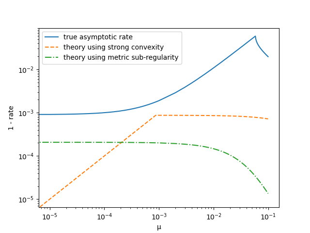
Figure 1: Comparison of the true rate (line above) and what is predicted by theory (2 lines below) for $a=0.03$, $\tau=\sigma=1$ and various values for $\mu$.

On Figure 1, we can see that there can be a large difference between what is predicted and what is observed, even for the simplest problem. Moreover, although the actual rate improves when $\mu$ increases, metric sub-regularity decreases, so that theory suggests the opposite of what is actually observed. On the other hand, using strong convexity explains the improvement of the rate when $\mu$ increases but does not manage to capture the linear convergence for $\mu=0$.

6 Quadratic error bound of the smoothed gap

We now introduce a new regularity assumption that truly generalized strongly convex-concave Lagrangians and smooth strongly convex objectives with linear constraints and is as broadly applicable as metric subregularity of the Lagrangian’s gradient.

6.1 Main assumption

Definition 4.

Given $\beta=(\beta_{x},\beta_{y})\in[0,+\infty]^{2}$, $z\in\mathcal{Z}$ and $\dot{z}\in\mathcal{Z}$, the smoothed gap $G_{\beta}$ is the function defined by

$$G_{\beta}(z;\dot{z})=\sup_{z^{\prime}\in\mathcal{Z}}L(x,y^{\prime})-L(x^{\prime},y)-\frac{\beta_{x}}{2\tau}\|x^{\prime}-\dot{x}\|^{2}-\frac{\beta_{y}}{2\sigma}\|y^{\prime}-\dot{y}\|^{2}\;.$$

We call the function $(z\mapsto G_{\beta}(z,\dot{z}))$ the smoothed gap centered at $\dot{z}$.

Although the smooth gap can be defined for any center $\dot{z}$, the next proposition shows that if $\dot{z}=z^{*}\in\mathcal{Z}^{*}$, then the smoothed gap is a measure of optimality.

Proposition 8.

Let $\beta\in[0,+\infty)^{2}$. If $z^{*}\in\mathcal{Z}^{*}$, then $z\in\mathcal{Z}^{*}\Leftrightarrow G_{\beta}(z;z^{*})=0$.

Proof.

We first remark that $G_{0}(z,z^{*})$ is the usual duality gap and that $G_{\infty}(z;z^{*})=L(x,y^{*})-L(x^{*},y)\geq 0$. Moreover, $G_{0}(z,z^{*})\geq G_{\beta}(z,z^{*})\geq G_{\infty}(z;z^{*})\geq 0$. Since $z\in\mathcal{Z}^{*}\Rightarrow G_{0}(z;z^{*})=0$, we have the implication $z\in\mathcal{Z}^{*}\Rightarrow G_{\beta}(z;z^{*})=0$.

For the converse implication, we denote

$$y_{\beta}(x) =\arg\max_{y^{\prime}}L(x,y^{\prime})-\frac{\beta_{y}}{2\sigma}\|y^{*}-y^{\prime}\|^{2}=\arg\max_{y^{\prime}}\langle Ax,y^{\prime}\rangle-g^{*}(y^{\prime})-g_{2}^{*}(y^{\prime})-\frac{\beta_{y}}{2\sigma}\|y^{*}-y^{\prime}\|^{2}$$

$$=\operatorname{prox}_{\sigma/\beta_{y}(g^{*}+g_{2}^{*})}\big{(}y^{*}+\frac{\sigma}{\beta}Ax\big{)}$$

By the strong convexity of the problem defining $G_{\beta}(\cdot;z^{*})$, we know that

$$\sup_{y^{\prime}}L(x,y^{\prime})-\frac{\beta_{y}}{2\sigma}\|y^{*}-y^{\prime}\|^{2} \geq L(x,y^{*})-\frac{\beta_{y}}{2\sigma}\|y^{*}-y^{*}\|^{2}+\frac{\beta_{y}}{2\sigma}\|y_{\beta}(x)-y^{*}\|^{2}\geq L(x^{*},y^{*})+\frac{\beta_{y}}{2\sigma}\|y_{\beta}(x)-y^{*}\|^{2}\;.$$

With a similar argument for $x_{\beta}(y)$, we get

$$G_{\beta}(z;z^{*})\geq\frac{\beta_{y}}{2\sigma}\|y_{\beta}(x)-y^{*}\|^{2}+\frac{\beta_{x}}{2\tau}\|x_{\beta}(y)-x^{*}\|^{2}\;.$$

Thus, if $G_{\beta}(z;z^{*})=0$, then $y_{\beta}(x)=y^{*}$ and $x_{\beta}(y)=x^{*}$.

$$y_{\beta}(x)=y^{*} \Leftrightarrow y^{*}=\operatorname{prox}_{\sigma/\beta_{y}(g^{*}+g_{2}^{*})}\big{(}y^{*}+\frac{\sigma}{\beta_{y}}Ax\big{)}$$

$$\Leftrightarrow 0\in y^{*}-(y^{*}+\frac{\sigma}{\beta_{y}}Ax)+\frac{\sigma}{\beta_{y}}\partial g^{*}(y^{*})+\frac{\sigma}{\beta_{y}}\nabla g_{2}^{*}(y^{*})$$

$$\Leftrightarrow 0\in-Ax+\partial g^{*}(y^{*})+\nabla g_{2}^{*}(y^{*})\Leftrightarrow x\in\mathcal{X}^{*}$$

and similarly $x_{\beta}(y)=x^{*}\Leftrightarrow y\in\mathcal{Y}^{*}$, which completes the proof of the proposition. ∎

Assumption 5.

There exists $\beta=(\beta_{x},\beta_{y})\in]0,+\infty]^{2}$, $\eta>0$ and a region $\mathcal{R}\subseteq\mathcal{Z}$ such that for all $z^{*}\in\mathcal{Z}^{*}$, $G_{\beta}(\cdot,z^{*})$ has a quadratic error bound with constant $\eta$ in the region $\mathcal{R}$ and with the norm $\|\cdot\|_{V}$. Said otherwise, for all $z\in\mathcal{R}$,

$$G_{\beta}(z;z^{*})\geq\frac{\eta}{2}\operatorname{dist}_{V}(z,\mathcal{Z}^{*})^{2}\;.$$

The next proposition, which is a simple consequence of [16, Prop. 1] says that even though QEB is a local concept, it can be extended to any compact set at the expense of degrading the constant.

Proposition 9.

If $G_{\beta}(\cdot,z^{*})$ has a $\eta$-QEB on $\{z:\operatorname{dist}(z,\mathcal{Z}^{*})_{V}<a\}$ then for all $M>1$, $G_{\beta}(\cdot,z^{*})$ has a $\frac{\eta}{M}$-QEB on $\{z:\operatorname{dist}(z,\mathcal{Z}^{*})_{V}<Ma\}$.

6.2 Problems with strong convexity

We now give a few examples to show that Assumption 5 is often satisfied.

Proposition 10.

If $L$ is $\mu$-strongly convex-concave in the norm $\|\cdot\|_{V}$, then $\forall z\in\mathcal{Z}$, $G_{\infty}(z;z^{*})\geq\frac{\mu}{2}\|z-z^{*}\|^{2}_{V}$.

Proof.

$G_{\infty}(z;z^{*})=L(x,y^{*})-L(x^{*},y)\geq\frac{\mu}{2}\|z-z^{*}\|^{2}_{V}$. ∎

Proposition 11.

If $f+f_{2}$ has a $L_{f}^{\prime}+L_{f}$-Lipschitz gradient, $g\square g_{2}=\iota_{\{b\}}$, the primal function $(x\mapsto f(x)+f_{2}(x)+g\square g_{2}(Ax))$ has a $\bar{\mu}$-QEB and $f+f_{2}$ is $\mu_{f}$-strongly convex, then the smoothed gap has a QEB:

$$G_{\beta}(z,z^{*})\geq\min\Big{(}\max\big{(}\frac{\tau\mu_{f}}{2},\frac{\bar{\mu}^{2}}{(L_{f}+L_{f}^{\prime})^{2}}\frac{\sigma\tau\sigma_{\min}(A)^{2}}{16\beta_{y}}\big{)},\frac{\sigma\sigma_{\min}(A)^{2}}{2(L_{f}+L_{f}^{\prime}+\beta_{x}/\tau)}\Big{)}\operatorname{dist}_{V}(z,\mathcal{Z}^{*})^{2}\;.$$

Note that we require either $\mu_{f}>0$ or $\bar{\mu}>0$.

Proof.

The proof is a generalization of Proposition 6 and reuses most of the argument.

$$\sup_{y^{\prime}\in\mathcal{Y}}L(x,y^{\prime})-\frac{\beta_{y}}{2\sigma}\|y^{\prime}-y^{*}\|^{2}=f(x){\color[rgb]{0,0,1}+f_{2}(x)}+\langle y^{*},Ax-b\rangle+\frac{\sigma}{2\beta_{y}}\|Ax-b\|^{2}\;.$$

We decompose $x=x_{A}+x_{A^{\perp}}$ with $x_{A^{\perp}}=P_{\{x^{\prime}:Ax^{\prime}=b\}}(x)$ and $x_{A}=x-x_{A^{\perp}}\in(\ker A)^{\perp}$. We have $Ax-b=Ax_{A}$, so that $\|Ax-b\|\geq\sigma_{\min}(A)\|x_{A}\|$. Moreover by convexity of $f{\color[rgb]{0,0,1}+f_{2}}$ and optimality condition $\nabla f(x^{*}){\color[rgb]{0,0,1}+\nabla f_{2}(x^{*})}=-A^{\top}y^{*}$,

$$f(x) {\color[rgb]{0,0,1}+f_{2}(x)}+\langle y^{*},Ax-b\rangle+\frac{\sigma}{2\beta_{y}}\|Ax-b\|^{2}$$

$$\geq f(x_{A^{\perp}}){\color[rgb]{0,0,1}+f_{2}(x_{A^{\perp}})}+\langle\nabla(f{\color[rgb]{0,0,1}+f_{2}})(x_{A^{\perp}}),x-x_{A^{\perp}}\rangle-\langle\nabla(f{\color[rgb]{0,0,1}+f_{2}})(x^{*}),x-x_{A^{\perp}}\rangle+\frac{\sigma}{2\beta_{y}}\sigma_{\min}(A)^{2}\|x_{A}\|^{2}$$

$$\geq f(x^{*}){\color[rgb]{0,0,1}+f_{2}(x^{*})}+\frac{\bar{\mu}}{2}\operatorname{dist}(x_{A^{\perp}},\mathcal{X}^{*})^{2}-(L_{f}+L_{f}^{\prime})\|x_{A^{\perp}}-x^{*}\|\|x_{A}\|+\frac{\sigma}{2\beta_{y}}\sigma_{\min}(A)^{2}\|x_{A}\|^{2}$$

where the last inequality comes from the assumption on the primal function and smoothness of $\nabla(f+f_{2})$. We combine this with

$$f(x){\color[rgb]{0,0,1}+f_{2}(x)}+\langle y^{*},Ax-b\rangle\geq f(x^{*}){\color[rgb]{0,0,1}+f_{2}(x^{*})}+\frac{\mu_{f}}{2}\operatorname{dist}(x,\mathcal{X}^{*})^{2}$$

to get for all $\lambda\in[0,1]$ and $\alpha>0$,

$$f(x) {\color[rgb]{0,0,1}+f_{2}(x)}+\langle y^{*},Ax-b\rangle+\frac{\sigma}{2\beta_{y}}\|Ax-b\|^{2}$$

$$\geq f(x^{*}){\color[rgb]{0,0,1}+f_{2}(x^{*})}+\big{(}\frac{\lambda\bar{\mu}}{2}-\frac{\lambda\alpha(L_{f}+L_{f}^{\prime})}{2}+\frac{(1-\lambda)\mu_{f}}{2}\big{)}\operatorname{dist}(x_{A^{\perp}},\mathcal{X}^{*})^{2}$$

$$\qquad\qquad+\big{(}\frac{\sigma}{2\beta_{y}}\sigma_{\min}(A)^{2}-\frac{\lambda(L_{f}+L_{f}^{\prime})}{2\alpha}+\frac{(1-\lambda)\mu_{f}}{2}\big{)}\|x_{A}\|^{2}$$

We take $\alpha=\frac{\bar{\mu}}{2(L_{f}+L_{f}^{\prime})}$, $\lambda=\frac{\bar{\mu}}{4(L_{f}+L_{f}^{\prime})^{2}}\frac{\sigma\sigma_{\min}(A)^{2}}{\beta_{y}}$ to get

$$f(x){\color[rgb]{0,0,1}+f_{2}(x)}+\langle y^{*},Ax-b\rangle+\frac{\sigma}{2\beta_{y}}\|Ax-b\|^{2}\geq f(x^{*}){\color[rgb]{0,0,1}+f_{2}(x^{*})}+\max\big{(}\frac{\mu_{f}}{2},\frac{\bar{\mu}^{2}}{(L_{f}+L_{f}^{\prime})^{2}}\frac{\sigma\sigma_{\min}(A)^{2}}{16\beta_{y}}\big{)}\operatorname{dist}(x,\mathcal{X}^{*})^{2}\;.$$ (7)

For the dual vector, we use the smoothness of the objective, the equality $\nabla f(x^{*}){\color[rgb]{0,0,1}+\nabla f_{2}(x^{*})}=-A^{\top}y^{*}$ and $Ax^{*}=b$.

$$-L(x^{\prime},y) =-f(x^{\prime}){\color[rgb]{0,0,1}-f_{2}(x^{\prime})}-\langle Ax^{\prime}-b,y\rangle$$

$$\geq-f(x^{*}){\color[rgb]{0,0,1}-f_{2}(x^{*})}-\langle\nabla f(x^{*})-\nabla f_{2}(x^{*}),x^{\prime}-x^{*}\rangle-\frac{L_{f}+L_{f}^{\prime}}{2}\|x^{\prime}-x^{*}\|^{2}-\langle Ax^{\prime}-b,y\rangle$$

$$=-L(x^{*},y^{*})+\langle A^{\top}y^{*},x^{\prime}-x^{*}\rangle-\langle x^{\prime}-x^{*},A^{\top}y\rangle-\frac{L_{f}+L_{f}^{\prime}}{2}\|x^{\prime}-x^{*}\|^{2}$$

For $a\in\mathbb{R}$, we restrict ourselves to $x^{\prime}=x^{*}+aA^{\top}(y^{*}-y)$ so that

$$\sup_{x^{\prime}\in\mathcal{X}}-L(x^{\prime},y)-\frac{\beta_{x}}{2\tau}\|x^{\prime}-x^{*}\|^{2} \geq\sup_{a\in\mathbb{R}}-L(x^{*}+aA^{\top}(y^{*}-y),y)-\frac{\beta_{x}a^{2}}{2\tau}\|A^{\top}(y^{*}-y)\|^{2}$$

$$\geq\sup_{a\in\mathbb{R}}-L(x^{*},y^{*})+(a-a^{2}\frac{L_{f}+L_{f}^{\prime}+\beta_{x}/\tau}{2})\|A^{\top}(y-y^{*})\|^{2}$$

$$=-L(x^{*},y^{*})+\frac{1}{2(L_{f}+L_{f}^{\prime}+\beta_{x}/\tau)}\|A^{\top}(y-y^{*})\|^{2}$$

Moreover, as in Proposition 6, we know that $\|A^{\top}y-A^{\top}y^{*}\|\geq\sigma_{\min(A)}\operatorname{dist}(y,\mathcal{Y}^{*})$, where $\sigma_{\min(A)}$ is the smallest singular value of $A$.

Combining this with (7) yields the result of the proposition. ∎

Proposition 12.

Suppose that $\mathcal{X}$ and $\mathcal{Y}$ are finite-dimensional. Suppose that $f,f_{2},g,g_{2}$ are convex piecewise linear-quadratic, which means that their domain is a union of polyhedra and on each of these polyhedra, they are quadratic functions. Then for all $\beta\in[0,+\infty[^{2}$, there exists $\eta(\beta)$ and $\mathcal{R}(\beta)$ such that $G_{\beta}(z;z^{*})\geq\frac{\eta(\beta)}{2}\operatorname{dist}_{V}(z,\mathcal{Z}^{*})^{2}$ for all $z\in\mathcal{R}(\beta)$ and $z^{*}\in\mathcal{Z}^{*}$.

Proof.

The proof follows the lines of [21]. The class of piecewise linear-quadratic functions is closed under scalar multiplication, addition, conjugation and Moreau envelope [28]. Hence for all $\beta\in[0,+\infty[^{2}$, $G_{\beta}(\cdot,z^{*})$ is piecewise linear quadratic. As a consequence, its subgradient $\partial_{z}G_{\beta}(\cdot,z^{*})$ is piecewise polyhedral and thus there exists $\eta>0$ such that it satisfies metric sub-regularity with constant $\eta$ at all $z^{*}\in\mathcal{Z}^{*}$ for 0 [11]. Since $G_{\beta}(\cdot,z^{*})$ is a convex function, this implies the result by Proposition 2. ∎

6.3 Linear programs

In the rest of the section, we are going to show that linear programs do satisfy Assumption 5 and give the constant as a function of the Hoffman constant [18].

We consider the linear optimization problem

$$\min_{x\in\mathbb{R}^{n}}c^{\top}x$$ (8)

$$A_{E,:}x=b_{E}$$

$$A_{I,:}x\leq b_{I}$$

$$x_{N}\geq 0$$

where $A$ is a $m\times n$ matrix, $b\in\mathbb{R}^{m}$, $E$ and $I$ are disjoint sets of indices such that $E\cup I=\{1,\ldots,m\}$ and $N$, $F$ are disjoint sets of indices such that $N\cup F=\{1,\ldots,n\}$.

A dual of this problem is given by

$$\max_{y\in\mathbb{R}^{m}}-b^{\top}y$$

$$(A_{:,F})^{\top}y+c_{F}=0$$

$$(A_{:,N})^{\top}y+c_{N}\geq 0$$

$$y_{I}\geq 0$$

It happens that the set of primal-dual solution of an LP is characterized by a system of linear equalities and inequalities. This holds true because a feasible primal-dual pair with equal values is necessarily optimal. We get the following system

$$\begin{cases}c^{\top}x+b^{\top}y=0\qquad\qquad&(A_{:,F})^{\top}y+c_{F}=0\\ A_{E,:}x=b_{E}&(A_{:,N})^{\top}y+c_{N}\geq 0\\ A_{I,:}x\leq b_{I}&y_{I}\geq 0\\ x_{N}\geq 0\end{cases}$$ (9)

Let us denote the Hoffman constant [18] of this system by $\theta$. This constant is the smallest positive number such that for all $z\in\mathbb{R}^{m+n}$

$$\operatorname{dist}(z,\mathcal{Z}^{*})\leq\theta\big{(} |c^{\top}x+b^{\top}y|^{2}+\|A_{E,:}x-b_{E}\|^{2}+\operatorname{dist}(A_{I,:}x-b_{I},\mathbb{R}^{I}_{-})^{2}$$

$$+\operatorname{dist}(x_{N},\mathbb{R}^{N}_{+})^{2}+\|(A_{:,F})^{\top}y+c_{F}\|^{2}$$

$$+\operatorname{dist}((A_{:,N})^{\top}y+c_{N},\mathbb{R}^{N}_{+})^{2}+\operatorname{dist}(y_{I},\mathbb{R}^{I}_{+})^{2}\big{)}^{1/2}$$ (10)

It is known that the Lagrangian’s subgradient of an LP satisfies metric sub-regularity with a constant proportional to $\theta$ [24]. We shall show that the same holds for the QEB of the smoothed gap centered at $z^{*}$.

Proposition 13.

For any $\beta\geq 0$, $R>0$ and $z^{*}\in\mathcal{Z}^{*}$, the linear program (8) satisfies the quadratic error bound: for all $z$ such that $G_{\beta}(z;z^{*})\leq R$, we have

$$G_{\beta}(z;z^{*})\geq\frac{\operatorname{dist}(z,\mathcal{Z}^{*})^{2}}{\theta^{2}\Big{(}\sqrt{\frac{2\beta}{\tau}}(\sqrt{2}+\|x_{F}^{*}\|+\|x_{N}^{*}\|)+\sqrt{\frac{2\beta}{\sigma}}(\sqrt{2}+\|y_{E}^{*}\|+\|y_{I}^{*}\|)+3\sqrt{R}\Big{)}^{2}}\;.$$

Hence, for $R$ of the order of $\frac{1}{\theta}$, $G_{\frac{1}{\theta}}(\cdot,z^{*})$ has a $\frac{c}{\theta}$-QEB with $c$ independent of $\theta$.

Proof.

See Appendix C. ∎

7 Analysis of PDHG under quadratic error bound of the smoothed gap

In this section, we show that under the new regularity assumption, PDHG converges linearly. Moreover, we give an explicit value for the rate. This result is central to the paper because it shows that the quadratic error bound of the smoothed gap is a fruitful assumption: not only it is as broadly applicable as the metric subregularity of the Lagrangian’s generalized gradient, but also the rates it predicts reach the state of the art in all subcases of interest.

Theorem 1.

Under Assumption 5, if $\mathcal{R}$ contains $\{z\;:\;\|z-P_{\mathcal{Z}^{*}}(z_{0})\|\leq\operatorname{dist}_{V}(z_{0},\mathcal{Z}^{*})\}$, then PDHG converges linearly at a rate

$$\Big{(}1+\Lambda\frac{\eta}{1+\eta/\lambda}\Big{)}\operatorname{dist}_{V}(z_{k+1},\mathcal{Z}^{*})^{2}\leq\operatorname{dist}_{V}(z_{k},\mathcal{Z}^{*})^{2}$$

where

$$\Lambda=\frac{\lambda}{\max((1+a_{2})\lambda+1/\beta_{x},(2+a_{2})\lambda+1/\beta_{y}),}$$

$\lambda$ is defined in Lemma 2 and $a_{2}=\max(\frac{2\alpha_{f}-1}{1-\alpha_{f}},\frac{2\alpha_{g}-1+\gamma}{1-\alpha_{g}-\gamma})\geq-1$ is defined in Lemma 4.

Proof.

In this proof, we will use the notation $\beta\odot z=(\beta_{x}x,\beta_{y}y)$ and $\|z\|_{\beta V}^{2}=\frac{\beta_{x}}{\tau}\|x\|^{2}+\frac{\beta_{y}}{\sigma}\|y\|^{2}$. By Lemma 4, we have

$$L(\bar{x}_{k+1},y)-L(x,\bar{y}_{k+1})\leq\frac{1}{2}\|z-z_{k}\|^{2}_{V}-\frac{1}{2}\|z-z_{k+1}\|^{2}_{V}+a_{2}\tilde{V}(\bar{z}_{k},z^{*})\;.$$

For $z^{*}=P_{\mathcal{Z}^{*}}(z_{k})$, the projection of $z_{k}$ onto the set of saddle points using norm $\|\cdot\|_{V}$,

$$G_{\beta}(\bar{z}_{k+1};z^{*}) =\sup_{x}\sup_{y}L(\bar{x}_{k+1},y)-\frac{\beta_{y}}{2}\|y-y^{*}\|^{2}_{\sigma^{-1}}-L(x,\bar{y}_{k+1})-\frac{\beta_{x}}{2}\|x-x^{*}\|^{2}_{\tau^{-1}}$$

$$\leq\sup_{z}\frac{1}{2}\|z-z_{k}\|^{2}_{V}-\frac{1}{2}\|z-z_{k+1}\|^{2}_{V}-\frac{1}{2}\|z-z^{*}\|_{\beta V}^{2}+a_{2}\tilde{V}(\bar{z}_{k},z^{*})$$

For the right hand side, we are looking for $z$ such that $\beta\odot(z-z^{*})+(z-z_{k+1})-(z-z_{k})=0$ so that $\beta\odot z=\beta\odot z^{*}+z_{k+1}-z_{k}$ and

$$\frac{1}{2}\|z-z_{k}\|^{2}_{V} -\frac{1}{2}\|z-z_{k+1}\|^{2}_{V}-\frac{1}{2}\|z-z^{*}\|_{\beta V}^{2}$$

$$=\frac{1}{2}\|z^{*}-z_{k}\|^{2}_{V}-\frac{1}{2}\|z^{*}-z_{k+1}\|^{2}_{V}+\frac{1}{2}\|z_{k+1}-z_{k}\|_{\beta^{-1}V}^{2}$$

$$\leq\frac{1}{2}\operatorname{dist}_{V}(z_{k},\mathcal{Z}^{*})^{2}-\frac{1}{2}\operatorname{dist}_{V}(z_{k+1},\mathcal{Z}^{*})^{2}+\frac{1}{2}\|z_{k+1}-z_{k}\|_{\beta^{-1}V}^{2}$$

where the last inequality comes from our choice of $z^{*}$. We also have by Lemma 2

$$\frac{1}{2}\operatorname{dist}_{V}(z_{k},\mathcal{Z}^{*})^{2}-\frac{1}{2}\operatorname{dist}_{V}(z_{k+1},\mathcal{Z}^{*})^{2}-\tilde{V}(z_{k},z^{*})\geq\frac{1}{2}\|z^{*}-z_{k}\|^{2}_{V}-\frac{1}{2}\|z^{*}-z_{k+1}\|^{2}_{V}-\tilde{V}(z_{k},z^{*})\geq 0\;.$$

Using Assumption 5, this leads to: $\forall\Lambda\in[0,1]$,

$$\frac{1}{2}\operatorname{dist}_{V}(z_{k},\mathcal{Z}^{*})^{2}-\frac{1}{2}\operatorname{dist}_{V}(z_{k+1},\mathcal{Z}^{*})^{2}+\frac{\Lambda}{2}\|z_{k}-z_{k+1}\|_{\beta^{-1}V}^{2}+(\Lambda a_{2}-(1-\Lambda))\tilde{V}(z_{k},z^{*})\geq\frac{\Lambda\eta}{2}\operatorname{dist}_{V}(\bar{z}_{k+1},\mathcal{Z}^{*})^{2}\;.$$

Using Lemma 5 and Lemma 3, we get, as soon as $\Lambda a_{2}-(1-\Lambda)\leq 0$,

$$\frac{1}{2}\operatorname{dist}_{V}( z_{k},\mathcal{Z}^{*})^{2}-\frac{1}{2}\operatorname{dist}_{V}(z_{k+1},\mathcal{Z}^{*})^{2}+\Big{(}\frac{\Lambda}{\beta_{x}}+(\Lambda a_{2}-(1-\Lambda))\lambda\Big{)}\frac{1}{2\tau}\|x_{k}-x_{k+1}\|^{2}$$

$$\qquad+\Big{(}\frac{\Lambda}{\beta_{y}}+(\alpha^{-1}-1)\Lambda\eta+(\Lambda a_{2}-(1-\Lambda))\lambda\Big{)}\frac{1}{2\sigma}\|y_{k}-y_{k+1}\|^{2}$$

$$\geq\frac{(1-\alpha)\Lambda\eta}{2}\operatorname{dist}_{V}(z_{k+1},\mathcal{Z}^{*})^{2}$$

So, taking $\alpha=\frac{\eta}{\lambda+\eta}$ and $\Lambda=\frac{\lambda}{\max((1+a_{2})\lambda+1/\beta_{x},(2+a_{2})\lambda+1/\beta_{y})}\leq 1$ leads to $\frac{\Lambda}{\beta_{y}}+(\alpha^{-1}-1)\Lambda\eta+(\Lambda a_{2}-(1-\Lambda))\lambda=\frac{\Lambda}{\beta_{y}}+\lambda\Lambda+(a_{2}+1)\lambda\Lambda-\lambda\leq 0$ and $\frac{\Lambda}{\beta_{x}}+(\Lambda a_{2}-(1-\Lambda))\lambda\leq 0$, so that

$$\operatorname{dist}_{V}(z_{k},\mathcal{Z}^{*})^{2} \geq\big{(}1+\Lambda\frac{\eta}{1+\eta/\lambda}\big{)}\operatorname{dist}_{V}(z_{k+1},\mathcal{Z}^{*})^{2}$$

and thus the algorithm enjoys a linear rate of convergence. ∎

Strongly convex-concave Lagrangian

If the Lagrangian is strongly convex concave, then we can take $\beta=(+\infty,+\infty)$ and $\eta=\mu$ (Proposition 10), so that we recover the rate of Proposition 5.

Note that in that case, the rate of order $1-c\mu$ given by Proposition 5, and so by its generalized version Theorem 1, is much better than what Proposition 7 tells us: a rate of order $1-c\mu^{2}$. Hence, we can see that for this important particular case, the rate predicted using the quadratic error bound of the smoothed gap is more informative than using the metric subregularity of the Lagrangian’s gradient. Moreover, the new assumption applies to all piecewise-linear quadratic problems, making it at the same time accurate and general.

Back to the toy problem

We consider again the linearly constrained 1D problem $\min_{x\in\mathbb{R}}\{\frac{\mu}{2}x^{2}\;:\;ax=b\}$ where $a,b\in\mathbb{R}$ and $\mu\geq 0$ introduced in Section 5.2 and we calculate the quadratic error bound of the smoothed gap.

$$G_{\beta}(\bar{z},z^{*}) =\sup_{y}\frac{\mu}{2}\bar{x}^{2}+y(a\bar{x}-b)-\frac{\beta_{y}}{2\sigma}(y-y^{*})^{2}+\sup_{x}-\frac{\mu}{2}x^{2}-\bar{y}(ax-b)-\frac{\beta_{x}}{2\tau}(x-x^{*})^{2}$$

$$=\frac{\mu}{2}\bar{x}^{2}+y^{*}(a\bar{x}-b)+\frac{\sigma}{2\beta_{y}}(a\bar{x}-b)^{2}+b\bar{y}+\frac{1}{2(\frac{\beta_{x}}{\tau}+\mu)}(\frac{\beta_{x}}{\tau}x^{*}+a\bar{y})^{2}-\frac{\beta_{x}}{2\tau}(x^{*})^{2}$$

$$\geq\frac{\mu\tau+\frac{\sigma\tau a^{2}}{\beta_{y}}}{2\tau}(\bar{x}-x^{*})^{2}+\frac{\sigma\tau a^{2}}{2\sigma(\beta_{x}+\mu\tau)}(\bar{y}-y^{*})^{2}$$

$$\geq\frac{1}{2}\min\Big{(}\mu\tau+\frac{\sigma\tau a^{2}}{\beta_{y}},\frac{\sigma\tau a^{2}}{\beta_{x}+\mu\tau}\Big{)}\|\bar{z}-z^{*}\|_{V}^{2}$$

As we have seen in Proposition 11, we can leverage the strong convexity of the objective. But also the smoothed gap may enjoy a quadratic error bound even if the objective is not strongly convex.

According to Theorem 1, since $2+a_{2}=\frac{1}{1-\tau\mu_{f}/2}$, the rate is $(1+\rho)^{-1}$ where

$$\rho=\Lambda\frac{\eta}{1+\eta/\lambda}=\frac{\lambda}{\max(\lambda\frac{\tau\mu_{f}}{1-\tau\mu_{f}/2}+1/\beta_{x},\lambda\frac{1+\tau\mu_{f}/2}{1-\tau\mu_{f}/2}+1/\beta_{y})}\frac{\min\Big{(}\mu\tau+\frac{\sigma\tau a^{2}}{\beta_{y}},\frac{\sigma\tau a^{2}}{\beta_{x}+\mu\tau}\Big{)}}{1+\min\Big{(}\mu\tau+\frac{\sigma\tau a^{2}}{\beta_{y}},\frac{\sigma\tau a^{2}}{\beta_{x}+\mu\tau}\Big{)}/\lambda}\;.$$

with $\lambda=(1-\mu\tau/2)(1-\sqrt{\sigma\tau a^{2}})$. Since the algorithm does not depend on $\beta_{x}$ or $\beta_{y}$ we can choose them so that they minimize the rate (or maximize $\rho$). On Figure 2, we can see that the rate of convergence explained using the quadratic error bound of the smoothed gap is as good as the rate using strong convexity (Assumption 3) when $\mu$ is large and does not vanish when $\mu$ goes to 0. On top of this, for small values of $\mu$, we obtain a much better rate than what is predicted using metric sub-regularity.

In Appendix D, Proposition 17, we derive a finer analysis in the case where we solve a linearly constrained problem whose objective function is strongly convex. Indeed, we can show that the largest singular value of the matrix $R$ described in Section 5.2 is $1-\gamma$. Yet, its spectral radius is much smaller. This implies that a contraction on $\operatorname{dist}_{V}(z_{k}-z^{*})^{2}$ is not enough to account for the actual rate. We propose to combine it with a contraction on $\|z_{k+1}-z_{k}\|^{2}_{V}$. The rationale for this addition is that for large strong convexity parameters, the primal sequence will behave as if it were tracking $\arg\min_{x^{\prime}}L(x^{\prime},y_{k})$. This is a kind of slow-fast system where the dual variable is slowly varying and the primal variable is fast.

When we plot the curve of the rate as a function of $\mu_{f}$ (with the legend “slow-fast double concentration rate”) we can see that this more complex analysis manages to explain the improvement of the rate for an increasing strong convexity parameter, together with its degradations when the parameter becomes too large.

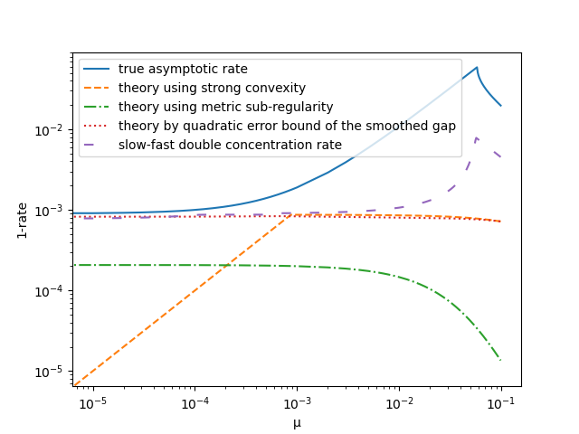
Figure 2: Comparison of the true rate $\rho$ (line above), what is predicted by theory using previous theories and what is predicted by using quadratic error bound of the smoothed gap for $a=0.03$, $\tau=\sigma=1$ and various values for $\mu$. We plot $1-\rho$ in logarithmic scale.

8 Restarted averaged primal-dual hybrid gradient

8.1 Restarted Averaged Primal-Dual Hybrid Gradient

In this section we will see how our new understanding of the rate of convergence of PDHG can help us design a faster algorithm.

Let averaged PDHG be given by Algorithm LABEL:APDHG. On the class of convex functions, averaged PDHG has an improved convergence speed in $O(1/k)$ in the worst case while PDHG has a convergence in $O(1/\sqrt{k})$ [10].

However, when averaging, we loose the linear convergence for well behaved problems. We thus propose to restart the algorithm as in Algorithm LABEL:RAPDHG. The following proposition shows that RAPDHG enjoys an improved rate of convergence where the product $\beta\eta$ is replaced by $\max(\beta,\eta)$. Hence for problems where $\eta(\beta)$ is a decreasing function of $\beta$, like linear programs, we will expect an improved convergence rate by averaging and restarting.

Proposition 14.

Under Assumption 5 with $\beta_{x}=\beta_{y}=\beta$, if the restart frequency $K$ satisfies $K\beta\geq 2$ and $K\eta\geq 2(2+a_{2}^{+})/\eta$, where $a_{2}^{+}=\max(0,a_{2})$ and $a_{2}$ is defined in Lemma 4, then RAPDHG converges linearly at a rate $2^{-1/K}$. Moreover, if $K=\lceil\max(2/\beta,2(2+a_{2}^{+})/\eta/\eta)\rceil$, then the rate is $\exp\Big{(}-\frac{1}{\lceil\max(2/\beta,2(2+a_{2}^{+})/\eta/\eta)\rceil}\ln(2)\Big{)}\approx\exp\Big{(}-\min(\beta/2,\eta/(2(2+a_{2}^{+})))\ln(2)\Big{)}$.

Proof.

Let us denote by $(z_{s}^{R})_{s\in\mathbb{N}}$ the iterates of RAPDHG. We keep the notation $z_{k},\bar{z}_{k}$ for the iterates of the inner loop.

Consider $z^{*}\in\mathcal{Z}^{*}$ and denote $a_{2}^{+}=\max(0,a_{2})$. We combine (6) with $a_{2}^{+}/2$ times (4) to get

$$L(\bar{x}_{k+1},y)-L(x,\bar{y}_{k+1}) \leq\frac{1}{2}\|z-z_{k}\|^{2}_{V}-\frac{1}{2}\|z-z_{k+1}\|^{2}_{V}+\frac{a_{2}^{+}}{2}\|z^{*}-z_{k}\|^{2}_{V}-\frac{a_{2}^{+}}{2}\|z^{*}-z_{k+1}\|^{2}_{V}+(a_{2}-a_{2}^{+})\tilde{V}(z_{k},z^{*})\;.$$

Summing this inequality for $k$ between $0$ and $K-1$, using the fact that the Lagrangian is convex-concave, and that $a_{2}-a_{2}^{+}\leq 0$, we get

$$L(\tilde{x}_{K},y)-L(x,\tilde{y}_{K})\leq\frac{1}{2K}\|z-z_{0}\|^{2}_{V}-\frac{1}{2K}\|z-z_{K}\|^{2}_{V}+\frac{a_{2}^{+}}{2K}\|z^{*}-z_{0}\|^{2}_{V}-\frac{a_{2}^{+}}{2K}\|z^{*}-z_{K}\|^{2}_{V}$$

which leads to

$$L(\tilde{x}_{K},y)-L(x,\tilde{y}_{K})-\frac{\beta}{2}\|z-z^{*}\|^{2}_{V}\leq\frac{1}{2K}\|z-z_{0}\|^{2}_{V}-\frac{\beta}{2}\|z-z^{*}\|^{2}_{V}+\frac{a_{2}^{+}}{2K}\|z^{*}-z_{0}\|^{2}_{V}$$

and so, as soon as $K\beta>1$, since the maximum of the right hand side is attained at $z=\frac{K\beta z^{*}-z_{0}}{K\beta-1}$,

$$G_{\beta}(\tilde{z}_{K},z^{*})\leq\frac{1}{2K}\Big{(}\frac{K\beta}{K\beta-1}+a_{2}^{+}\Big{)}\|z^{*}-z_{0}\|^{2}_{V}\;.$$

We now use Assumption 5 to get

$$\frac{1}{K}\Big{(}\frac{K\beta}{K\beta-1}+a_{2}^{+}\Big{)}\|z^{*}-z_{0}\|^{2}_{V}\geq\eta\|z^{*}-\tilde{z}_{K}\|^{2}\;.$$

We choose $z^{*}=P_{\mathcal{Z}^{*}}(z_{0})$ and $K$ such that $K\beta\geq 2$ and $K\eta\geq 2(2+a_{2}^{+})$ in order to get

$$\operatorname{dist}_{V}(z_{1}^{R},\mathcal{Z}^{*})^{2}=\operatorname{dist}_{V}(\tilde{z}_{K},\mathcal{Z}^{*})^{2}\leq\frac{1}{2}\operatorname{dist}_{V}(z_{0},\mathcal{Z}^{*})^{2}\;.$$

If we choose $K=\lceil\max(2/\beta,2(2+a_{2}^{+})/\eta)\rceil$ we thus get a linear convergence

$$\operatorname{dist}_{V}(z_{s}^{R},\mathcal{Z}^{*})^{2} \leq\frac{1}{2^{s}}\operatorname{dist}_{V}(\tilde{z}_{0}^{R},\mathcal{Z}^{*})^{2}$$

$$\leq\exp\Big{(}-\frac{1}{\lceil\max(2/\beta,2(2+a_{2}^{+})/\eta)\rceil}\ln(2)\Big{)}^{sK}\operatorname{dist}_{V}(z_{0},\mathcal{Z}^{*})^{2}$$

where $sK$ is the total number of iterations. ∎

The rate of convergence of RAPDHG has two nice features as compared to plain PDHG. Indeed, there is a factor $\Lambda$ in Theorem 1 in front of the quadratic error bound constant $\eta$, which is of order $\lambda\beta$ when $\beta$ is small. On the other hand, the rate of RAPDHG has no direct dependence on $\lambda$, which means that it will behave well even if $\sigma\tau\|A\|^{2}$ is close to 1. Moreover, it replaces $\beta\eta$ by $\min(\beta,\eta)$, which will be orders of magnitude better in the case of linear programs where $\eta=O(\beta)$ for $\beta=1/\theta$ (Proposition 13)

8.2 Self-centered smoothed gap

In this paper, we have shown that the smoothed gap is a convenient quantity for the analysis of PDHG and that assuming that it satisfies a quadratic error bound condition explains well its behaviour. However, since computing it requires the knowledge of a saddle point, one cannot use the smoothed gap for algorithmic design, and in particular for the tuning of RAPDHG.

We thus propose the following approximation, that we call the self-centered smoothed gap.

Definition 5.

Given $\beta=(\beta_{x},\beta_{x})\in[0,+\infty[^{2}$, and $z\in\mathcal{Z}$, the self-centered smoothed gap is given by $G_{\beta}(z,z)$.

The motivation for this definition is the following lemma.

Lemma 6.

For all $z,\dot{z}\in\mathcal{Z}$ and $z^{*}$ equal to the projection of $\dot{z}$ onto $\mathcal{Z}^{*}$,

$$G_{\beta}(z,\dot{z})\geq G_{2\beta}(z,z^{*})-\beta\operatorname{dist}_{V}(\dot{z},\mathcal{Z}^{*})^{2}_{V}\;.$$ (11)

Proof.

$$G_{\beta}(z,\dot{z}) =\max_{z^{\prime}}L(x,y^{\prime})-L(x^{\prime},y)-\frac{\beta}{2}\|\dot{z}-z^{\prime}\|^{2}_{V}$$

$$\geq\max_{z^{\prime}}L(x,y^{\prime})-L(x^{\prime},y)-\beta\|z^{*}-z^{\prime}\|^{2}_{V}-\beta\|\dot{z}-z^{*}\|^{2}_{V}$$

$$=G_{2\beta}(z,z^{*})-\beta\|\dot{z}-z^{*}\|^{2}_{V}=G_{2\beta}(z,z^{*})-\beta\operatorname{dist}_{V}(\dot{z},\mathcal{Z}^{*})^{2}_{V}\qed$$ (12)

This shows that $G_{\beta}(z,\dot{z})$ is a good approximation to the measure of optimality $G_{2\beta}(z,z^{*})$ as soon as $\beta$ is small enough or $\dot{z}$ is close enough to $z^{*}$. It happens that for $\dot{z}=z$, we can prove even more.

Proposition 15.

The self-centered smoothed gap is a measure of optimality. Indeed, $\forall z\in\mathcal{Z}$, $\forall\beta\in[0,+\infty[^{2}$:

1. $G_{\beta}(z,z)\geq 0$.

2. $G_{\beta}(z,z)=0\Leftrightarrow z\in\mathcal{Z}^{*}$.

3. For $z^{*}=P_{\mathcal{Z}^{*}}(z)\in\mathcal{Z}^{*}$, if $G_{\beta}(z,z^{*})\geq\frac{\eta}{2}\operatorname{dist}_{V}(z,\mathcal{Z}^{*})^{2}$, then we have $G_{\beta^{\prime}}(z,z)\geq\frac{\eta^{\prime}}{2}\operatorname{dist}_{V}(z,\mathcal{Z}^{*})^{2}$ where $\beta^{\prime}=\min(\beta/2,\eta/4)$ and $\eta^{\prime}=\eta/2$.

Proof.

The function $\Phi:z^{\prime}\mapsto L(x,y^{\prime})-L(x^{\prime},y)-\frac{\beta}{2}\|z-z^{\prime}\|^{2}_{V}$ is $\beta$-strongly concave in the norm $\|\cdot\|_{V}$ so for $z^{*}_{\beta}(z)=\arg\max\Phi$, we have

$$G_{\beta}(z,z)=\max_{z^{\prime}}\Phi(z^{\prime})\geq\Phi(z)+\frac{\beta}{2}\|z^{*}_{\beta}(z)-z\|^{2}_{V}\;.$$

Using the fact that $\Phi(z)=0$ gives point $\mathbf{i}$.

For the second point, it is clear by Proposition 8 that $G_{\beta}(z^{*},z^{*})=0$. For the converse implication, we shall do the proof only for $\beta>0$ because $G_{0}(z,z)$ is the usual duality gap.

$$G_{\beta}(z,z)=0\;\Rightarrow\;\frac{\beta}{2}\|z^{*}_{\beta}(z)-z\|^{2}_{V}=0\;\Rightarrow\;z^{*}_{\beta}(z)=z\;\Rightarrow\;\begin{cases}0\in-\partial_{x}L(x,y)-\frac{\beta}{\tau}(x-x)\\ 0\in-\partial_{y}(-L)(x,y)-\frac{\beta}{\sigma}(y-y)\end{cases}\Rightarrow z\in\mathcal{Z}^{*}$$

so that point $\mathbf{ii}$ holds.

Finally, suppose that $G_{\beta}(z,z^{*})\geq\frac{\eta}{2}\operatorname{dist}_{V}(z,\mathcal{Z}^{*})^{2}$. Since $\beta^{\prime}=\min(\beta/2,\eta(\beta)/4)\leq\beta/2$, we have $G_{2\beta^{\prime}}(z,z^{*})\geq G_{\beta}(z,z^{*})$. Using Lemma 6, we have

$$G_{\beta^{\prime}}(z,z) \geq G_{2\beta^{\prime}}(z,z^{*})-\beta^{\prime}\operatorname{dist}_{V}(z,\mathcal{Z}^{*})^{2}\geq G_{\beta}(z,z^{*})-\beta^{\prime}\operatorname{dist}_{V}(z,\mathcal{Z}^{*})^{2}\geq\big{(}\frac{\eta}{2}-\beta^{\prime}\big{)}\operatorname{dist}_{V}(z,\mathcal{Z}^{*})^{2}$$

$$\geq\frac{\eta}{4}\operatorname{dist}_{V}(z,\mathcal{Z}^{*})^{2}\;.\qed$$

In the numerical experiment section, we shall use the self-centered smoothed gap as a stopping criterion with $\beta=(0,\delta)$ where $\delta$ is the dual infeasibility.

8.3 Adaptive restart

We now modify RAPDHG so that instead of using unknown quantities $\beta$ and $\eta$ to set the restart period $K$, we monitor the self-centered smoothed gap and restart when this quantity has been halved. In order to take into account cases where averaging is detrimental, we then compare $\tilde{z}_{k}$ and $\bar{z}_{k}$ and restart at the best of these in terms of smoothed gap. This adaptive restart is formalized in Algorithm 4 and justified by the following proposition.

Proposition 16.

Suppose that Assumption 5 holds, i.e., there exists $\beta,\eta$ such that for all $z^{*}\in\mathcal{Z}^{*}$ and $z$ verifying $\operatorname{dist}_{V}(z,\mathcal{Z}^{*})\leq\operatorname{dist}_{V}(z_{0},\mathcal{Z}^{*})$ we have $G_{\beta}(z;z^{*})\leq\frac{\eta}{2}\operatorname{dist}_{V}(z,\mathcal{Z}^{*})$. Denote $\eta^{\prime}(\beta^{\prime})=0$ if $\beta^{\prime}\geq\min(\beta/2,\eta/4)$ and $\eta^{\prime}(\beta^{\prime})=\eta$ otherwise. Then, as soon as $\beta_{s}\leq\min(\beta/2,\eta/4)$ the iterates of Algorithm 4 satisfy for all $\beta^{\prime}\in]0,+\infty[$,

$$G_{\beta^{\prime}}(\tilde{z}_{k},\tilde{z}_{k})\leq\frac{2}{(k-s)\eta^{\prime}(\beta_{s})}\big{(}2+a_{2}^{+}+\frac{2}{(k-s)\beta^{\prime}}\big{)}G_{\beta_{s}}(z_{s},z_{s})\;.$$

where $a_{2}^{+}=\max(0,a_{2})$ and $a_{2}$ is defined in Lemma 4.

Proof.

As in Proposition 14, we have $\forall z$,

$$L(\tilde{x}_{k},y)-L(x,\tilde{y}_{k})\leq\frac{1}{2(k-s)}\|z-z_{s}\|^{2}_{V}-\frac{1}{2(k-s)}\|z-z_{k}\|^{2}_{V}+\frac{a_{2}^{+}}{2(k-s)}\|z^{*}-z_{s}\|^{2}_{V}-\frac{a_{2}^{+}}{2(k-s)}\|z^{*}-z_{k}\|^{2}_{V}$$

Summing (6) for $l$ between $s$ and $k-1$ and using the fact that the Lagrangian is convex-concave, we get for all $z$, We go on with

$$L(\tilde{x}_{k},y)-L(x,\tilde{y}_{k})-\frac{\beta^{\prime}}{2}\|z-\tilde{z}_{k}\|^{2}_{V}\leq\frac{1}{2(k-s)}\|z-z_{s}\|^{2}_{V}-\frac{1}{2(k-s)}\|z-z_{k}\|^{2}_{V}-\frac{\beta^{\prime}}{2}\|z-\tilde{z}_{k}\|^{2}_{V}$$

$$\hskip 200.0003pt+\frac{a_{2}^{+}}{2(k-s)}\|z^{*}-z_{s}\|^{2}_{V}-\frac{a_{2}^{+}}{2(k-s)}\|z^{*}-z_{k}\|^{2}_{V}$$

$$G_{\beta^{\prime}}(\tilde{z}_{k},\tilde{z}_{k})\leq\sup_{z}\frac{1}{2(k-s)}\|z-z_{s}\|^{2}_{V}-\frac{1}{2(k-s)}\|z-z_{k}\|^{2}_{V}-\frac{\beta^{\prime}}{2}\|z-\tilde{z}_{k}\|^{2}_{V}$$

$$\hskip 200.0003pt+\frac{a_{2}^{+}}{2(k-s)}\|z^{*}-z_{s}\|^{2}_{V}-\frac{a_{2}^{+}}{2(k-s)}\|z^{*}-z_{k}\|^{2}_{V}$$

This supremum is attained at $z=\tilde{z}_{k}+\frac{1}{\beta^{\prime}(k-s)}(z_{k}-z_{s})$ so that, denoting $z^{*}=P_{\mathcal{Z}^{*}}(z_{s})$,

$$G_{\beta^{\prime}}(\tilde{z}_{k},\tilde{z}_{k}) \leq\frac{1}{2(k-s)}\big{\langle}z_{k}-z_{s},2\tilde{z}_{k}+\frac{1}{\beta^{\prime}(k-s)}(z_{k}-z_{s})-z_{k}-z_{s}\big{\rangle}_{V}-\frac{1}{2\beta^{\prime}(k-s)^{2}}\|z_{k}-z_{s}\|^{2}_{V}$$

$$\hskip 200.0003pt+\frac{a_{2}^{+}}{2(k-s)}\|z^{*}-z_{s}\|^{2}_{V}-\frac{a_{2}^{+}}{2(k-s)}\|z^{*}-z_{k}\|^{2}_{V}$$

$$\leq\frac{1}{2(k-s)}\|\tilde{z}_{k}-z_{s}\|^{2}_{V}-\frac{1}{2(k-s)}\|\tilde{z}_{k}-z_{k}\|^{2}_{V}+\frac{1}{2\beta^{\prime}(k-s)^{2}}\|z_{k}-z_{s}\|^{2}_{V}$$

$$\hskip 200.0003pt+\frac{a_{2}^{+}}{2(k-s)}\|z^{*}-z_{s}\|^{2}_{V}-\frac{a_{2}^{+}}{2(k-s)}\|z^{*}-z_{k}\|^{2}_{V}$$

$$\leq\frac{1}{k-s}\|\tilde{z}_{k}-z^{*}\|^{2}_{V}+\frac{1}{k-s}\|z_{s}-z^{*}\|^{2}_{V}-0+\frac{1}{\beta^{\prime}(k-s)^{2}}\|z_{k}-z^{*}\|^{2}_{V}+\frac{1}{\beta^{\prime}(k-s)^{2}}\|z_{s}-z^{*}\|^{2}_{V}$$

$$\hskip 200.0003pt+\frac{a_{2}^{+}}{2(k-s)}\|z^{*}-z_{s}\|^{2}_{V}-\frac{a_{2}^{+}}{2(k-s)}\|z^{*}-z_{k}\|^{2}_{V}$$

$$\leq\frac{1}{k-s}\|\tilde{z}_{k}-z^{*}\|^{2}_{V}+\Big{(}\frac{1}{k-s}+\frac{1}{\beta^{\prime}(k-s)^{2}}+\frac{a_{2}^{+}}{2(k-s)}\Big{)}\|z_{s}-z^{*}\|^{2}_{V}+\Big{(}\frac{1}{\beta^{\prime}(k-s)^{2}}-\frac{a_{2}^{+}}{2(k-s)}\Big{)}\|z_{k}-z^{*}\|^{2}_{V}$$

$$\leq\frac{1}{k-s}\Big{(}2+a_{2}^{+}+\frac{2}{\beta^{\prime}(k-s)}\Big{)}\operatorname{dist}_{V}(z_{s},\mathcal{Z}^{*})^{2}$$

because Lemma 2 implies that $\|z_{k}-z^{*}\|\leq\|z_{s}-z^{*}\|$ for all $k\geq s$, and thus also $\|\tilde{z}_{k}-z^{*}\|\leq\|z_{s}-z^{*}\|$. We now use the quadratic error bound of the self-centered smoothed gap, which holds thanks to Proposition 15.

$$G_{\beta^{\prime}}(\tilde{z}_{k},\tilde{z}_{k}) \leq\frac{2}{\eta^{\prime}(\beta_{s})(k-s)}\Big{(}2+a_{2}^{+}+\frac{2}{\beta^{\prime}(k-s)}\Big{)}G_{\beta_{s}}(z_{s},z_{s})\;.\qed$$

Hence, choosing $\beta^{\prime}=\frac{1}{k-s}$, as soon as $k-s\geq\frac{4(4+a_{2}^{+})}{\eta^{\prime}(\beta_{s})}$, we have $G_{\beta^{\prime}}(\tilde{z}_{k},\tilde{z}_{k})\leq 0.5G_{\beta_{s}}(z_{s},z_{s})$. We have added additional safeguards – $\beta^{\prime}=\min(\frac{1}{k-s+1},\beta_{s}/2)$ and $G_{\beta_{s}}(z_{s},z_{s})\leq 0.01\min(G_{\beta^{\prime}}(\tilde{z}_{k+1},\tilde{z}_{k+1}),G_{\beta^{\prime}}(\bar{z}_{k+1},\bar{z}_{k+1}))$ – for cases where a precipitous restart may lead to $\beta^{\prime}>\min(\beta/2,\eta/4)$ and thus slow down the algorithm afterwards because we have lost control on $\eta(\beta^{\prime})$.

  $s=0$, $\beta_{0}>0$

  for $k\in\mathbb{N}$ do

     $z_{k+1}=T(z_{k})$   – see (3)

     $\tilde{z}_{k+1}=\frac{1}{k-s+1}\sum_{l=s+1}^{k+1}\bar{z}_{l}$

     $\beta^{\prime}=\min(\frac{1}{k-s+1},2\beta_{s})$

     $G^{\mathrm{c}urr}=\min(G_{\beta^{\prime}}(\tilde{z}_{k+1},\tilde{z}_{k+1}),G_{\beta^{\prime}}(\bar{z}_{k+1},\bar{z}_{k+1}))$

     if $G^{\mathrm{c}urr}\leq 0.5\;G_{\beta_{s}}(z_{s},z_{s})$ or $G_{\beta_{s}}(z_{s},z_{s})\leq 0.01\;G^{\mathrm{c}urr}$  then

        if $G_{\beta^{\prime}}(\tilde{z}_{k+1},\tilde{z}_{k+1})\leq G_{\beta^{\prime}}(\bar{z}_{k+1},\bar{z}_{k+1})$ then

           Reassign $z_{k+1}\leftarrow\tilde{z}_{k+1}$

        else

           Keep current iterate

        $z_{s}=z_{k+1}$

        $\beta_{s}=\beta^{\prime}$

        $s=k$

Algorithm 4 RAPDHG with adaptive restart

9 Numerical experiments

In the last section, we present some numerical experiments to illustrate the linear convergence behaviour of PDHG and RAPDHG. We will first look at a two linear program to show that the linear rate of RAPDHG can be much faster than PDHG’s. Then, we will exemplify the limits of the methods with a ridge regression problem where restarted averaging does not help and a non-polyhedral problem where we do not observe a linear rate of convergence.

9.1 Small linear program

The first experiment is on a small LP where the dual optimal set is known:

$$\min_{x\in\mathbb{R}^{4},x\geq 0}-7x_{1}-9x_{2}-18x_{3}-17x_{4}$$

$$2x_{1}+4x_{2}+6x_{3}+7x_{4}\leq 41$$

$$x_{1}+x_{2}+2x_{3}+2x_{4}\leq 17$$

$$x_{1}+2x_{2}+3x_{3}+3x_{4}\leq 24$$

To give an estimate the quadratic error bound constant, we compute for several values of $\beta$ the quantity $\hat{\eta}(\beta)=\min_{k}\frac{G_{\beta}(z_{k};z^{*})}{0.5\operatorname{dist}(z_{k},\mathcal{Z}^{*})^{2}}$. We can do it because $\mathcal{Z}^{*}$ is known for this small problem. Using a similar idea we can also get an estimate of the metric subregularity constant of the Lagrangian’s gradient, here $\eta\approx 0.0187$.

On Figure 3, we can see that the actual rate of convergence is rather close to what is predicted by theory. Moreover, RAPDHG is much faster than PDHG. Yet, note that thousands of iterations for a LP with 4 variables and 3 constraints is not competitive with the state of the art.

$\beta$	$\hat{\eta}(\beta)$
1	0.00018
0.1	0.00183
0.01	0.01829
0.001	0.14474

Figure 3: Table: Estimates of the quadratic error bound of the smoothed gap for several smoothing parameters. Figure: Comparison of PDHG and RAPDHG on the small linear program. The restart period of 200 was chosen because for $\beta=1/100$, we have $\hat{\eta}(\beta)\approx 2/100$, so that $K=\lceil\max(2/\beta,4/\eta)\rceil=200$.

9.2 Larger polyhedral problem

We then run an experiment on a more realistic problem. We run PDHG and RAPDHG with adaptive restart on the following sparse SVM problem:

$$\min_{w\in\mathbb{R}^{d}}\sum_{i=1}^{n}\max(0,1-y_{i}x_{i,:}w)+\|w\|_{1}$$

where $(y_{i},x_{i,:})_{1\leq i\leq n}$ are the data points from the a1a dataset [7] ($d=119$ and $n=1,605$). We normalized the data matrix so that $\|x_{:,j}\|_{2}=1$.

The convergence profile is given in Figure 4. The behaviour of the algorithms is similar to what was seen in the small size problem. Here however, we can see clearly two phases. In the beginning, we observe a sublinear convergence, where restart and averaging does not help. Then the linear rate kicks in after a nonnegligible time. We believe that it comes from something related to the condition $G_{\beta}(z;z^{*})\leq R$ in Proposition 13. Note that this cold start phase is quite long. On our laptop computer with 4 Intel(R) Core(TM) i5-7200U CPU @ 2.50GHz it took 5.7s while the adaptive proximal point method of [24] took 0.93s to solve the problem.

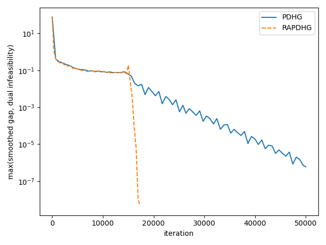
Figure 4: Comparison of PDHG and RAPDHG: sparse SVM on the a1a dataset. We are plotting the optimality measure for the last iterate

9.3 Ridge regression

In this experiment, we test on a problem where restarting does not help. We consider least squares with $\ell_{2}$ regularization

$$\min_{x}\frac{1}{2}\|Ax-b\|^{2}+50\|x\|^{2}$$

where $A$ and $b$ are given by the real-sim dataset [7]. Since we know the strong convexity-concavity parameter of the Lagrangian, we choose the step sizes $\sigma$ and $\tau$ as in Section 5.1. As a consequence, PDHG has a convergence rate that matches the theoretical lower bound for this class problem and cannot be improved.

We can see on Figure 5 that, as expected, restart and averaging does not help: $\bar{z}_{k}$ is consistently better than $\tilde{z}_{k}$ so that RAPDHG with adaptive restart selects the same sequence as PDHG and the the two curves match. We added a comparison with restarted-FISTA [15] to show that the choice of step sizes indeed suffices to get an algorithm with accelerated rate.

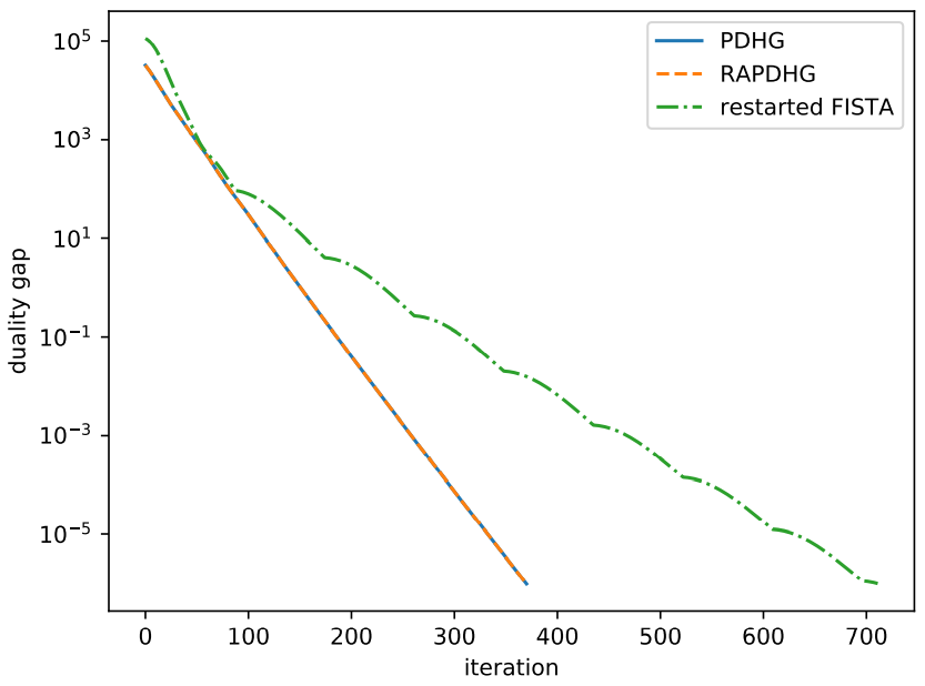
Figure 5: Solving $\ell_{2}$ regularized least squares on the real-sim dataset.

9.4 TV-L1

We consider the minimization of the following non-polyhedral function

$$\min_{x}\lambda\|x-I\|_{1}+\|Dx\|_{2,1}$$

where $I$ is the Cameraman image, $D$ is the 2D discrete gradient, $\|z\|_{2,1}=\sum_{p\in P}\sqrt{z_{p,1}^{2}+z_{p,2}^{2}}$ and $\lambda=1.9$. This problem is not piecewise linear-quadratic, so that our linear convergence result does not hold. Yet is rather structured: it is equivalent to a second order cone program. We can see in Figure 6 that this is a difficult problem for PDHG but that RAPDHG does improve the convergence speed significantly. The solution we obtain is shown in Figure 7.

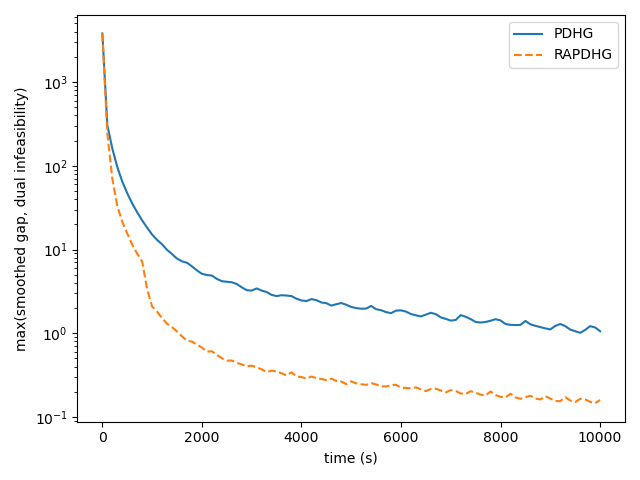
Figure 6: Comparison of PDHG and RAPDHG on the $\ell_{1}$ ROF problem.

Figure 7: Left:original image – Right: solution, 59% of the pixels are unchanged

10 Conclusion

In this paper, we have tried to understand the linear rate of convergence of primal-dual hybrid gradient. Even on a very simple problem, we have seen that current regularity assumptions are not sufficient to explain the behavior of the algorithm. We have then introduced the quadratic error bound of the smoothed gap and argue that this new condition is more widely applicable and more precise than previous ones. Finally, we showed how this new knowledge can be used to improve the algorithm.

This work opens several perspectives:

• Can the quadratic error bound of the smooth gap be used to understand better the convergence rate of other primal-dual algorithms? Interesting cases would be the ADMM, the augmented Lagrangian method and coordinate update methods to cite a few.

• We have seen in (11) that the smoothed gap at a non-optimal point can approximate the smoothed gap at an optimal point. Considering it as a stopping criterion would be an alternative to the KKT error, which implicitly requires metric sub-regularity to make sense, and duality gap, which is $+\infty$ nearly everywhere for linearly constrained problems.

• Our first attempt for the design of a primal-dual algorithm with an improved linear rate of convergence has shown the usefulness of our regularity assumption. Would we be able to design an optimal algorithm for the class of problems with a given quadratic error bound of the smoothed gap function?

Appendix A Proofs of Section 3

$\triangleright$ Lemma 1  Let $p=\operatorname{prox}_{\tau f}(x)$ and $p^{\prime}=\operatorname{prox}_{\tau f}(x^{\prime})$ where $f$ is $\mu_{f}$-strongly convex. For all $x$ and $x^{\prime}$,

$$f(p)+\frac{1}{2\tau}\|p-x\|^{2}\leq f(x^{\prime})+\frac{1}{2\tau}\|x^{\prime}-x\|^{2}-\frac{1{\color[rgb]{0.7,0.35,0}+\tau\mu_{f}}}{2\tau}\|p-x^{\prime}\|^{2}$$

$${\color[rgb]{0.7,0.35,0}(1+2\tau\mu_{f})}\|p-p^{\prime}\|^{2}\leq\|x^{\prime}-x\|^{2}-\|p-x-p^{\prime}+x^{\prime}\|^{2}$$

Proof.

$p=\arg\min_{z}f(z)+\frac{1}{2\tau}\|z-x\|^{2}$

Yet, $h:z\mapsto f(z)+\frac{1}{2\tau}\|z-x\|^{2}-\frac{1{\color[rgb]{0.7,0.35,0}+\tau\mu_{f}}}{2\tau}\|p-z\|^{2}$ is convex and $0\in\partial h(p)$. This implies the first inequality by Fermat’s rule.

We now apply the first inequality at $(x,p^{\prime})$ and at $(x^{\prime},p)$ and then sum.

$$f(p)+\frac{1}{2\tau}\|p-x\|^{2}+f(p^{\prime})+\frac{1}{2\tau}\|p^{\prime}-x^{\prime}\|^{2}\leq f(p^{\prime})+\frac{1}{2\tau}\|p^{\prime}-x\|^{2}-\frac{1{\color[rgb]{0.7,0.35,0}+\tau\mu_{f}}}{2\tau}\|p-p^{\prime}\|^{2}+f(p)\\ +\frac{1}{2\tau}\|p-x^{\prime}\|^{2}-\frac{1{\color[rgb]{0.7,0.35,0}+\tau\mu_{f}}}{2\tau}\|p^{\prime}-p\|^{2}$$

Rearranging the squared norm terms we get

$${\color[rgb]{0.7,0.35,0}(1+\tau\mu_{f})}\|p^{\prime}-p\|^{2}\leq\langle p-p^{\prime},x-x^{\prime}\rangle$$

$$\|p-x-p^{\prime}+x^{\prime}\|^{2}=\|p-p^{\prime}\|^{2}+\|x-x^{\prime}\|^{2}-2\langle p-p^{\prime},x-x^{\prime}\rangle\leq\|x-x^{\prime}\|^{2}-{\color[rgb]{0.7,0.35,0}(1+2\tau\mu_{f})}\|p-p^{\prime}\|^{2}$$

∎

$\triangleright$ Lemma 2  Let $T:\mathcal{X}\times\mathcal{Y}\to\mathcal{X}\times\mathcal{Y}$ be defined for any $(x,y)$ by (3). Suppose that $\nabla f_{2}$ is $L_{f}$-Lipschitz continuous and $\nabla g_{2}^{*}$ is $L_{g^{*}}$-Lipschitz continuous. If the step sizes satisfy $\gamma=\sigma\tau\|A\|^{2}<1$, $\tau L_{f}/2\leq\alpha_{f}<1$, $\alpha_{g}=\sigma L_{g^{*}}/2\leq 1$ and $\sigma L_{g^{*}}/2\leq\alpha_{f}(1-\sigma\tau\|A\|^{2})$ then $T$ is nonexpansive in the norm $\|\cdot\|_{V}$,

$$\|T(z)-T(z^{\prime})\|^{2}_{V}{\color[rgb]{0.7,0.35,0}+2\mu_{f}\|\bar{x}-\bar{x}^{\prime}\|^{2}+2\mu_{g^{*}}\|\bar{y}-\bar{y}^{\prime}\|^{2}} \leq\|z-z^{\prime}\|_{V}^{2}-2\tilde{V}(z,z^{\prime})$$ (13)

and $T$ is $\frac{1}{1+\lambda}$-averaged where

$$\lambda ={\color[rgb]{0,0,1}1-\alpha_{f}-\frac{\alpha_{g}-(1-\gamma)\alpha_{f}}{2}-\sqrt{(1-\alpha_{f})^{2}\gamma+((1-\gamma)\alpha_{f}-\alpha_{g})^{2}/4}}\geq(1-\sqrt{\gamma}){\color[rgb]{0,0,1}(1-\alpha_{f})}\;,$$

which means for $z=(x,y)$ and $z^{\prime}=(x^{\prime},y^{\prime})$

$$\|T(z)-T(z^{\prime})\|^{2}_{V}{\color[rgb]{0.7,0.35,0}+2\mu_{f}\|\bar{x}-\bar{x}^{\prime}\|^{2}+2\mu_{g^{*}}\|\bar{y}-\bar{y}^{\prime}\|^{2}}\leq\|z-z^{\prime}\|_{V}^{2}-\lambda\|z-T(z)-z^{\prime}+T(z^{\prime})\|^{2}_{V}\;.$$ (14)

As a consequence, $(z_{k})$ converges to a saddle point of the Lagrangian.

Proof.

In the appendix, we will improve slightly the result in the case where $f$ or $g^{*}$ is strongly convex. Note that all what follows works even if $\mu_{f}=\mu_{g^{*}}=0$.

Since the proximal operator of a convex function is firmly nonexpansive, for $(x,y)$, $(x^{\prime},y^{\prime})\in\mathcal{Z}$,

$${\color[rgb]{0.7,0.35,0}(1+2\mu_{f}\tau)}\|\bar{x}-\bar{x}^{\prime}\|^{2} \leq\|x{\color[rgb]{0,0,1}-\tau\nabla f_{2}(x)}-\tau A^{\top}y-x^{\prime}{\color[rgb]{0,0,1}+\tau\nabla f_{2}(x^{\prime})}+\tau A^{\top}y^{\prime}\|^{2}$$

$$\qquad\qquad-\|x{\color[rgb]{0,0,1}-\tau\nabla f_{2}(x)}-\tau A^{\top}y-\bar{x}-x^{\prime}{\color[rgb]{0,0,1}+\tau\nabla f_{2}(x^{\prime})}+\tau A^{\top}y^{\prime}+\bar{x}^{\prime}\|^{2}$$

$$=\|x{\color[rgb]{0,0,1}-\tau\nabla f_{2}(x)}-x^{\prime}{\color[rgb]{0,0,1}+\tau\nabla f_{2}(x^{\prime})}\|^{2}+\tau^{2}\|A^{\top}(y-y^{\prime})\|^{2}$$

$$\qquad\qquad-2\tau\langle x{\color[rgb]{0,0,1}-\tau\nabla f_{2}(x)}-x^{\prime}{\color[rgb]{0,0,1}+\tau\nabla f_{2}(x^{\prime})},A^{\top}(y-y^{\prime})\rangle$$

$$\qquad\qquad-\|x{\color[rgb]{0,0,1}-\tau\nabla f_{2}(x)}-\bar{x}-x^{\prime}{\color[rgb]{0,0,1}+\tau\nabla f_{2}(x^{\prime})}+\bar{x}^{\prime}\|^{2}-\tau^{2}\|A^{\top}(y-y^{\prime})\|^{2}$$

$$\qquad\qquad+2\tau\langle x{\color[rgb]{0,0,1}-\tau\nabla f_{2}(x)}-\bar{x}-x^{\prime}{\color[rgb]{0,0,1}+\tau\nabla f_{2}(x^{\prime})}+\bar{x}^{\prime},A^{\top}(y-y^{\prime})\rangle$$

$$=\|x{\color[rgb]{0,0,1}-\tau\nabla f_{2}(x)}-x^{\prime}{\color[rgb]{0,0,1}+\tau\nabla f_{2}(x^{\prime})}\|^{2}-\|x{\color[rgb]{0,0,1}-\tau\nabla f_{2}(x)}-\bar{x}-x^{\prime}{\color[rgb]{0,0,1}+\tau\nabla f_{2}(x^{\prime})}+\bar{x}^{\prime}\|^{2}$$

$$\qquad\qquad-2\tau\langle\bar{x}-\bar{x}^{\prime},A^{\top}(y-y^{\prime})\rangle$$

We also have

$$\|x{\color[rgb]{0,0,1}-\tau\nabla f_{2}(x)}-x^{\prime}{\color[rgb]{0,0,1}+\tau\nabla f_{2}(x^{\prime})}\|^{2} =\|x-x^{\prime}\|^{2}+\tau^{2}\|\nabla f_{2}(x)-\nabla f_{2}(x^{\prime})\|^{2}-2\tau\langle\nabla f_{2}(x)-\nabla f_{2}(x^{\prime}),x-x^{\prime}\rangle$$

$$\leq\|x-x^{\prime}\|^{2}-\big{(}\frac{2\tau}{L_{f}}-\tau^{2}\big{)}\|\nabla f_{2}(x)-\nabla f_{2}(x^{\prime})\|^{2}$$

$$\|x-\tau\nabla f_{2}(x) -\bar{x}-x^{\prime}+\tau\nabla f_{2}(x^{\prime})+\bar{x}^{\prime}\|^{2}=\|x-\bar{x}-x^{\prime}+\bar{x}^{\prime}\|^{2}+\tau^{2}\|\nabla f_{2}(x)-\nabla f_{2}(x^{\prime})\|^{2}$$

$$\qquad\qquad-2\tau\langle\nabla f_{2}(x)-\nabla f_{2}(x^{\prime}),x-x^{\prime}-\bar{x}+\bar{x}^{\prime}\rangle$$

$$\geq(1-\alpha_{f})\|x-\bar{x}-x^{\prime}-\bar{x}^{\prime}\|^{2}+\tau^{2}(1-\alpha_{f}^{-1})\|\nabla f_{2}(x)-\nabla f_{2}(x^{\prime})\|^{2}$$

for all $\alpha_{f}>0$. Hence,

$${\color[rgb]{0.7,0.35,0}(1+2\mu_{f}\tau)}\|\bar{x}-\bar{x}^{\prime}\|^{2}\leq\|x-x^{\prime}\|^{2} -(1-\alpha_{f})\|x-\bar{x}-x^{\prime}+\bar{x}^{\prime}\|^{2}-2\tau\langle\bar{x}-\bar{x}^{\prime},A^{\top}(y-y^{\prime})\rangle$$

$$-\big{(}\frac{2\tau}{L_{f}}-\alpha_{f}^{-1}\tau^{2}\big{)}\|\nabla f_{2}(x)-\nabla f_{2}(x^{\prime})\|^{2}$$

Similarly,

$${\color[rgb]{0.7,0.35,0}(1+2\mu_{g^{*}}\sigma)}\|\bar{y}-\bar{y}^{\prime}\|^{2}\leq\|y-y^{\prime}\|^{2} -{\color[rgb]{0,0,1}(1-\alpha_{g})}\|y-\bar{y}-y^{\prime}+\bar{y}^{\prime}\|^{2}+2\sigma\langle\bar{y}-\bar{y}^{\prime},A(\bar{x}-\bar{x}^{\prime})\rangle$$

$${\color[rgb]{0,0,1}-\big{(}\frac{2\sigma}{L_{g^{*}}}-\alpha_{g}^{-1}\sigma^{2}\big{)}\|\nabla g_{2}(y)-\nabla g_{2}(y^{\prime})\|^{2}}$$

We then proceed to

$$\|T(x,y)-T(x^{\prime},y^{\prime})\|^{2}_{V} =\frac{1}{\tau}\|\bar{x}-\tau A^{\top}(\bar{y}-y)-\bar{x}^{\prime}+\tau A^{\top}(\bar{y}^{\prime}-y^{\prime})\|^{2}+\frac{1}{\sigma}\|\bar{y}-\bar{y}^{\prime}\|^{2}$$

$$=\frac{1}{\tau}\|\bar{x}-\bar{x}^{\prime}\|^{2}+\tau\|A^{\top}(\bar{y}-y)-A^{\top}(\bar{y}^{\prime}-y^{\prime})\|^{2}$$

$$\qquad-2\langle\bar{x}-\bar{x}^{\prime},A^{\top}(\bar{y}-y)-A^{\top}(\bar{y}^{\prime}-y^{\prime})\rangle+\frac{1}{\sigma}\|\bar{y}-\bar{y}^{\prime}\|^{2}$$

$$\leq\frac{1}{\tau}\|x-x^{\prime}\|^{2}-\frac{1{\color[rgb]{0,0,1}-\alpha_{f}}}{\tau}\|x-\bar{x}-x^{\prime}+\bar{x}^{\prime}\|^{2}-2\langle\bar{x}-\bar{x}^{\prime},A^{\top}(y-y^{\prime})\rangle$$

$$\qquad+\tau\|A^{\top}(\bar{y}-y-\bar{y}^{\prime}+y^{\prime})\|^{2}-2\langle\bar{x}-\bar{x}^{\prime},A^{\top}(\bar{y}-y)-A^{\top}(\bar{y}^{\prime}-y^{\prime})\rangle$$

$$\qquad+\frac{1}{\sigma}\|y-y^{\prime}\|^{2}-\frac{1{\color[rgb]{0,0,1}-\alpha_{g}}}{\sigma}\|y-\bar{y}-y^{\prime}+\bar{y}^{\prime}\|^{2}+2\langle\bar{y}-\bar{y}^{\prime},A(\bar{x}-\bar{x}^{\prime})\rangle$$

$$\qquad{\color[rgb]{0,0,1}-\big{(}\frac{2\tau}{L_{f}}-\alpha_{f}^{-1}\tau^{2}\big{)}\|\nabla f_{2}(x)-\nabla f_{2}(x^{\prime})\|^{2}}{\color[rgb]{0.7,0.35,0}-2\mu_{f}\|\bar{x}-\bar{x}^{\prime}\|^{2}}$$

$$\qquad{\color[rgb]{0,0,1}-\big{(}\frac{2\sigma}{L_{g^{*}}}-\alpha_{g}^{-1}\sigma^{2}\big{)}\|\nabla g_{2}(y)-\nabla g_{2}(y^{\prime})\|^{2}}{\color[rgb]{0.7,0.35,0}-2\mu_{g^{*}}\|\bar{y}-\bar{y}^{\prime}\|^{2}}$$

We choose $\alpha_{f}=\tau L_{f}/2<1$ and $\alpha_{g}=\sigma L_{g^{*}}/2<1$ and we note that $-2\langle\bar{x}-\bar{x}^{\prime},A^{\top}(y-y^{\prime})\rangle-2\langle\bar{x}-\bar{x}^{\prime},A^{\top}(\bar{y}-y)-A^{\top}(\bar{y}^{\prime}-y^{\prime})\rangle+2\langle\bar{y}-\bar{y}^{\prime},A(\bar{x}-\bar{x}^{\prime})\rangle=0$. This leads to

$$\|T(x,y)-T(x^{\prime},y^{\prime})\|^{2}_{V} \leq\|z-z^{\prime}\|^{2}_{V}-\frac{1-{\color[rgb]{0,0,1}\alpha_{f}}}{\tau}\|x-\bar{x}-x^{\prime}+\bar{x}^{\prime}\|^{2}-\frac{1-{\color[rgb]{0,0,1}\alpha_{g}}-\tau\sigma\|A\|^{2}}{\sigma}\|y-\bar{y}-y^{\prime}+\bar{y}^{\prime}\|^{2}$$

$$\qquad{\color[rgb]{0.7,0.35,0}-2\mu_{f}\|\bar{x}-\bar{x}^{\prime}\|^{2}}{\color[rgb]{0.7,0.35,0}-2\mu_{g^{*}}\|\bar{y}-\bar{y}^{\prime}\|^{2}}$$

which proves (4). Now, we shall prove that $V(z,z^{\prime})\geq\frac{\lambda}{2}\|z-T(z)-z^{\prime}+T(z^{\prime})\|^{2}_{V}$. For any $\lambda\in[0,1{\color[rgb]{0,0,1}-\alpha_{f}}]$ and $\alpha>0$,

$$\|T(x,y)-T(x^{\prime},y^{\prime})\|^{2}_{V} \leq\frac{1}{\tau}\|x-x^{\prime}\|^{2}-\frac{1{\color[rgb]{0,0,1}-\alpha_{f}}-\lambda}{\tau}\|x-\bar{x}-x^{\prime}+\bar{x}^{\prime}\|^{2}$$

$$\qquad-\frac{\lambda}{\tau}\|x-\bar{x}+\tau A^{\top}(\bar{y}-y)-x^{\prime}+\bar{x}^{\prime}-\tau A^{\top}(\bar{y}^{\prime}-y^{\prime})\|^{2}$$

$$\qquad+\lambda\tau\|A^{\top}(\bar{y}-y-\bar{y}^{\prime}+y^{\prime})\|^{2}$$

$$\qquad+2\lambda\langle x-\bar{x}-x^{\prime}+\bar{x}^{\prime},A^{\top}(\bar{y}-y)-A^{\top}(\bar{y}^{\prime}-y^{\prime})\rangle$$

$$\qquad+\frac{1}{\sigma}\|y-y^{\prime}\|^{2}-\frac{1{\color[rgb]{0,0,1}-\alpha_{g}}-\sigma\tau\|A\|^{2}}{\sigma}\|y-\bar{y}-y^{\prime}+\bar{y}^{\prime}\|^{2}$$

$$\qquad{\color[rgb]{0.7,0.35,0}-2\mu_{f}\|\bar{x}-\bar{x}^{\prime}\|^{2}}{\color[rgb]{0.7,0.35,0}-2\mu_{g^{*}}\|\bar{y}-\bar{y}^{\prime}\|^{2}}$$

$$\|T(x,y)-T(x^{\prime},y^{\prime})\|^{2}_{V} \leq\frac{1}{\tau}\|x-x^{\prime}\|^{2}+\frac{1}{\sigma}\|y-y^{\prime}\|^{2}$$

$$\qquad-\frac{\lambda}{\tau}\|x-\bar{x}+\tau A^{\top}(\bar{y}-y)-x^{\prime}+\bar{x}^{\prime}-\tau A^{\top}(\bar{y}^{\prime}-y^{\prime})\|^{2}$$

$$\qquad-\frac{\lambda}{\sigma}\|y-\bar{y}-y^{\prime}+\bar{y}^{\prime}\|^{2}+(\frac{\lambda}{\tau\alpha}-\frac{1{\color[rgb]{0,0,1}-\alpha_{f}}-\lambda}{\tau})\|x-\bar{x}-x^{\prime}+\bar{x}^{\prime}\|^{2}$$

$$\qquad+\Big{(}(1+\lambda+\lambda\alpha)\tau\|A\|^{2}-\frac{1{\color[rgb]{0,0,1}-\alpha_{g}}-\lambda}{\sigma}\Big{)}\|(\bar{y}-y-\bar{y}^{\prime}+y^{\prime})\|^{2}$$

$$\qquad{\color[rgb]{0.7,0.35,0}-2\mu_{f}\|\bar{x}-\bar{x}^{\prime}\|^{2}}{\color[rgb]{0.7,0.35,0}-2\mu_{g^{*}}\|\bar{y}-\bar{y}^{\prime}\|^{2}}$$

where $\lambda\in[0,1{\color[rgb]{0,0,1}-\alpha_{f}}]$ and $\alpha>0$ are arbitrary. We choose $\lambda$ and $\alpha$ such that

$$\frac{\lambda}{\alpha}=1{\color[rgb]{0,0,1}-\alpha_{f}}-\lambda$$

$$(1+\lambda+\lambda\alpha)\gamma=1{\color[rgb]{0,0,1}-\alpha_{g}}-\lambda$$

that is $\lambda=1-\sqrt{\gamma}$ and $\alpha=\frac{\lambda}{1-\lambda}=\frac{1-\sqrt{\gamma}}{\sqrt{\gamma}}$ when $f_{2}=0$ and $g_{2}=0$. In the case $f_{2}$ and $g_{2}$ non zero, we take

$$\lambda=1-\alpha_{f}-\frac{\alpha_{g}-(1-\gamma)\alpha_{f}}{2}-\sqrt{(1-\alpha_{f})^{2}\gamma+((1-\gamma)\alpha_{f}-\alpha_{g})^{2}/4}\;,\qquad\alpha=\frac{\lambda}{1-\alpha_{f}-\lambda}\;.$$

Note that as soon as $\alpha_{g}\leq(1-\gamma)\alpha_{f}$, we have $(1-\alpha_{f})(1-\sqrt{\gamma})\leq\lambda\leq 1-\alpha_{f}$. We continue as

$$\|T(x,y)-T(x^{\prime},y^{\prime})\|^{2}_{V}\leq\frac{1}{\tau}\|x-x^{\prime}\|^{2}+\frac{1}{\sigma}\|y-y^{\prime}\|^{2}-\frac{\lambda}{\tau}\|x-\bar{x}+\tau A^{\top}(\bar{y}-y)-x^{\prime}+\bar{x}^{\prime}-\tau A^{\top}(\bar{y}^{\prime}-y^{\prime})\|^{2}\\ -\frac{\lambda}{\sigma}\|y-\bar{y}-y^{\prime}+\bar{y}^{\prime}\|^{2}{\color[rgb]{0.7,0.35,0}-2\mu_{f}\|\bar{x}-\bar{x}^{\prime}\|^{2}-2\mu_{g^{*}}\|\bar{y}-\bar{y}^{\prime}\|^{2}}\;.$$

We get that $T$ is $\beta$-averaged with $\frac{1-\beta}{\beta}=\lambda$, that is $\beta=\frac{1}{\lambda+1}$.

For the convergence, we use Krasnosels’kii Mann theorem [4]. ∎

$\triangleright$ Lemma 3  For any $z^{*}\in\mathcal{Z}^{*}$, $\tilde{V}$ satisfies

$$\tilde{V}(z_{k},z^{*})=\frac{1-\alpha_{f}}{2\tau}\|\bar{x}_{k+1}-x_{k}\|^{2}+(\frac{1-\alpha_{g}}{2\sigma}-\frac{\tau\|A\|^{2}}{2})\|\bar{y}_{k+1}-y_{k}\|^{2}\geq\frac{\lambda}{2}\|z_{k+1}-z_{k}\|^{2}_{V}\;.$$

Proof.

The last part of the proof of Lemma 2 shows that for any $z,z^{\prime}\in\mathcal{Z}$,

$$V(z,z^{\prime})\geq\frac{\lambda}{2}\|z-T(z)-z^{\prime}+T(z^{\prime})\|^{2}_{V}$$

Since $T(z^{*})=z^{*},T(z_{k})=z_{k+1}$, we get the desired result. ∎

$\triangleright$ Lemma 4  Suppose that $\gamma=\sigma\tau\|A\|^{2}<1$, $\tau L_{f}/2\leq\alpha_{f}<1$, $\alpha_{g}=\sigma L_{g^{*}}/2\leq 1$ and $\sigma L_{g^{*}}/2\leq\alpha_{f}(1-\sigma\tau\|A\|^{2})$. For all $k\in\mathbb{N}$ and for all $z\in\mathcal{Z}$,

$$L(\bar{x}_{k+1},y)-L(x,\bar{y}_{k+1}) {\color[rgb]{0.7,0.35,0}+\frac{1}{2}\|\bar{z}_{k+1}-z\|^{2}_{\mu}}\leq\frac{1}{2}\|z-z_{k}\|^{2}_{V{\color[rgb]{0.7,0.35,0}-\mu_{2}}}-\frac{1}{2}\|z-z_{k+1}\|^{2}_{V}$$

$$+{\color[rgb]{0,0,1}a_{2}}\tilde{V}(z_{k},z^{*})$$

where $\tilde{V}(z_{k},z^{*})=(\frac{1}{2\tau}-\frac{L_{f}}{2})\|\bar{x}_{k+1}-x_{k}\|^{2}+(\frac{1}{2\sigma}-\frac{\tau\|A\|^{2}}{2}-\frac{L_{g^{*}}}{2})\|\bar{y}_{k+1}-y_{k}\|^{2}$ and $a_{2}=\max(\frac{2\alpha_{f}-1}{1-\alpha_{f}},\frac{2\alpha_{g}-1+\gamma}{1-\alpha_{g}-\gamma})$. $a_{2}\geq-1$ may be positive or negative.

Proof.

By Taylor-Lagrange inequality and convexity of $f_{2}$ and $g_{2}^{*}$,

$$f_{2}(\bar{x}_{k+1})\leq f_{2}(x_{k})+\langle\nabla f_{2}(x_{k}),\bar{x}_{k+1}-x_{k}\rangle+\frac{L_{f}}{2}\|\bar{x}_{k+1}-x_{k}\|^{2}$$

$$\qquad\qquad\leq f_{2}(x)+\langle\nabla f_{2}(x_{k}),\bar{x}_{k+1}-x\rangle+\frac{L_{f}}{2}\|\bar{x}_{k+1}-x_{k}\|^{2}{\color[rgb]{0.7,0.35,0}-\frac{\tau\mu_{f_{2}}}{\tau}\|x_{k}-x\|^{2}}$$

$$g_{2}^{*}(\bar{y}_{k+1})\leq g_{2}^{*}(y_{k})+\langle\nabla g_{2}^{*}(y_{k}),\bar{y}_{k+1}-y_{k}\rangle+\frac{L_{g^{*}}}{2}\|\bar{y}_{k+1}-y_{k}\|^{2}$$

$$\qquad\qquad\leq g_{2}^{*}(y)+\langle\nabla g_{2}^{*}(y_{k}),\bar{y}_{k+1}-y\rangle+\frac{L_{g^{*}}}{2}\|\bar{y}_{k+1}-y_{k}\|^{2}{\color[rgb]{0.7,0.35,0}-\frac{\sigma\mu_{g_{2}^{*}}}{\sigma}\|y_{k}-y\|^{2}}$$

By definitions of $\bar{x}_{k+1}$ and $\bar{y}_{k+1}$, for all $x\in\mathcal{X}$ and $y\in\mathcal{Y}$, we have:

$$f(\bar{x}_{k+1})\leq f(x)+\langle{\color[rgb]{0,0,1}\nabla f_{2}(x_{k})}+A^{\top}y_{k},x-\bar{x}_{k+1}\rangle+\frac{1}{2\tau}\|x-x_{k}\|^{2}-\frac{1{\color[rgb]{0.7,0.35,0}+\tau\mu_{f}}}{2\tau}\|x-\bar{x}_{k+1}\|^{2}-\frac{1}{2\tau}\|\bar{x}_{k+1}-x_{k}\|^{2}$$

$$g^{*}(\bar{y}_{k+1})\leq g^{*}(y)+\langle{\color[rgb]{0,0,1}\nabla g^{*}_{2}(y_{k})}-A\bar{x}_{k+1},y-\bar{y}_{k+1}\rangle+\frac{1}{2\sigma}\|y-y_{k}\|^{2}-\frac{1+{\color[rgb]{0.7,0.35,0}\sigma\mu_{g*}}}{2\sigma}\|y-\bar{y}_{k+1}\|^{2}-\frac{1}{2\sigma}\|\bar{y}_{k+1}-y_{k}\|^{2}$$

Summing these inequalities and using the relations $x_{k+1}=\bar{x}_{k+1}-\tau A^{\top}(\bar{y}_{k+1}-y_{k})$ and $y_{k+1}=\bar{y}_{k+1}$ yields

$$L(\bar{x}_{k+1},y) -L(x,\bar{y}_{k+1})=f(\bar{x}_{k+1}){\color[rgb]{0,0,1}+f_{2}(\bar{x}_{k+1})}+\langle A\bar{x}_{k+1},y\rangle-g^{*}(y){\color[rgb]{0,0,1}-g_{2}^{*}(y)}-f(x){\color[rgb]{0,0,1}-f_{2}(x)}$$

$$\qquad-\langle Ax,\bar{y}_{k+1}\rangle+g^{*}(\bar{y}_{k+1}){\color[rgb]{0,0,1}+g_{2}^{*}(\bar{y}_{k+1})}$$

$$\leq\frac{1{\color[rgb]{0.7,0.35,0}-\tau\mu_{f_{2}}}}{2\tau}\|x-x_{k}\|^{2}+\frac{1{\color[rgb]{0.7,0.35,0}-\sigma\mu_{g_{2}^{*}}}}{2\sigma}\|y-y_{k}\|^{2}-\frac{1}{2\tau}\|x-x_{k+1}\|^{2}-\frac{1}{2\sigma}\|y-y_{k+1}\|^{2}$$

$$\qquad-\frac{1}{2\tau}\|x_{k+1}-\bar{x}_{k+1}\|^{2}-\frac{1}{\tau}\langle x-x_{k+1},x_{k+1}-\bar{x}_{k+1}\rangle$$

$$\qquad+\langle A\bar{x}_{k+1},y\rangle-\langle Ax,\bar{y}_{k+1}\rangle+\langle A^{\top}y_{k},x-\bar{x}_{k+1}\rangle-\langle A\bar{x}_{k+1},y-\bar{y}_{k+1}\rangle$$

$$\qquad-\frac{1}{2\tau}\|\bar{x}_{k+1}-x_{k}\|^{2}+\frac{1}{2\sigma}\|\bar{y}_{k+1}-y_{k}\|^{2}{\color[rgb]{0,0,1}+\frac{L_{f}}{2}\|\bar{x}_{k+1}-x_{k}\|^{2}+\frac{L_{g^{*}}}{2}\|\bar{y}_{k+1}-y_{k}\|^{2}}$$

$$\qquad{\color[rgb]{0.7,0.35,0}-\frac{\tau\mu_{f}}{2\tau}\|\bar{x}_{k+1}-x\|^{2}}{\color[rgb]{0.7,0.35,0}-\frac{\sigma\mu_{g^{*}}}{2\sigma}\|\bar{y}_{k+1}-y\|^{2}}$$

$$=\frac{1}{2}\|z-z_{k}\|^{2}_{V{\color[rgb]{0.7,0.35,0}-\mu_{2}}}-\frac{1}{2}\|z-z_{k+1}\|^{2}_{V}-\frac{\tau}{2}\|A^{\top}(\bar{y}_{k+1}-y_{k})\|^{2}$$

$$\qquad+\langle x-\bar{x}_{k+1}+\tau A^{\top}(\bar{y}_{k+1}-y_{k}),A^{\top}(\bar{y}_{k+1}-y_{k})\rangle+\langle A(\bar{x}_{k+1}-x),\bar{y}_{k+1}-y\rangle$$

$$\qquad-\frac{1}{2}\|\bar{z}_{k+1}-z_{k}\|^{2}_{V}{\color[rgb]{0,0,1}+\frac{L_{f}}{2}\|\bar{x}_{k+1}-x_{k}\|^{2}+\frac{L_{g^{*}}}{2}\|\bar{y}_{k+1}-y_{k}\|^{2}}{\color[rgb]{0.7,0.35,0}-\frac{1}{2}\|\bar{z}_{k+1}-z\|^{2}_{\mu}}$$

$$=\frac{1}{2}\|z-z_{k}\|^{2}_{V}-\frac{1}{2}\|z-z_{k+1}\|^{2}_{V}+\frac{\tau}{2}\|A^{\top}(\bar{y}_{k+1}-y_{k})\|^{2}-\frac{1}{2}\|\bar{z}_{k+1}-z_{k}\|^{2}_{V}$$

$$\qquad{\color[rgb]{0,0,1}+\frac{L_{f}}{2}\|\bar{x}_{k+1}-x_{k}\|^{2}+\frac{L_{g^{*}}}{2}\|\bar{y}_{k+1}-y_{k}\|^{2}}{\color[rgb]{0.7,0.35,0}-\frac{1}{2}\|\bar{z}_{k+1}-z\|^{2}_{\mu}}$$

Since $\tilde{V}(z_{k},z^{*})=\frac{1-\alpha_{f}}{2\tau}\|\bar{x}_{k+1}-x_{k}\|^{2}+(\frac{1-\alpha_{g}-\gamma}{2\sigma})\|\bar{y}_{k+1}-y_{k}\|^{2}$, $\alpha_{f}\geq\frac{\tau L_{f}}{2}$ and $\alpha_{g}=\frac{\sigma L_{g^{*}}}{2}$, we can write

$$\frac{\tau}{2}\|A^{\top}(\bar{y}_{k+1}-y_{k})\|^{2} -\frac{1}{2}\|\bar{z}_{k+1}-z_{k}\|^{2}_{V}{\color[rgb]{0,0,1}+\frac{L_{f}}{2}\|\bar{x}_{k+1}-x_{k}\|^{2}+\frac{L_{g^{*}}}{2}\|\bar{y}_{k+1}-y_{k}\|^{2}}$$

$$\leq\frac{1}{2\tau}(2\alpha_{f}-1)\|\bar{x}_{k+1}-x_{k}\|^{2}+\frac{1}{2\sigma}(\gamma+2\alpha_{g}-1)\|\bar{y}_{k+1}-y_{k}\|^{2}$$

$$\leq\max\big{(}\frac{2\alpha_{f}-1}{1-\alpha_{f}},\frac{\gamma+2\alpha_{g}-1}{1-\gamma-\alpha_{g}}\big{)}\tilde{V}(z_{k},z^{*})$$

Hence,

$$L(\bar{x}_{k+1},y) -L(x,\bar{y}_{k+1})\leq\frac{1}{2}\|z-z_{k}\|^{2}_{V{\color[rgb]{0.7,0.35,0}-\mu_{2}}}-\frac{1}{2}\|z-z_{k+1}\|^{2}_{V}+a_{2}\tilde{V}(z_{k},z^{*}){\color[rgb]{0.7,0.35,0}-\frac{1}{2}\|\bar{z}_{k+1}-z\|^{2}_{\mu}}$$

where $a_{2}=\max(\frac{2\alpha_{f}-1}{1-\alpha_{f}},\frac{\gamma+2\alpha_{g}-1}{1-\gamma-\alpha_{g}})\geq-1$ may be negative or positive. ∎

$\triangleright$ Proposition 4  Let $z_{0}\in\mathcal{Z}$ and let $R\subseteq\mathcal{Z}$. If $\sigma\tau\|A\|^{2}{\color[rgb]{0,0,1}+\sigma L_{g^{*}}}\leq 1$ and $\tau L_{f}\leq 1$ then we have the stability

$$\|z_{k}-z^{*}\|_{V}\leq\|z_{0}-z^{*}\|_{V}$$

for all $z^{*}\in\mathcal{Z}^{*}$.

Define $\tilde{z}_{k}=\frac{1}{k}\sum_{l=1}^{k}\bar{z}_{l}$ and the restricted duality gap $G(\bar{z},R)=\sup_{z\in R}L(\bar{x},y)-L(x,\bar{y})$. We have the sublinear iteration complexity

$$G(\tilde{z}_{k},R)\leq\frac{1}{2k}\sup_{z\in R}\|z-z_{0}\|^{2}_{V}\;.$$

Proof.

For any $z^{*}\in\mathcal{Z}^{*}$, $L(\bar{x}_{k+1},y^{*})-L(x^{*},\bar{y}_{k+1})\geq 0$ which implies by Lemma 4 the stability inequality, since $a_{2}\leq 0$ in the case $\alpha_{f}\leq\frac{1}{2}$ and $2\alpha_{g}+\gamma\leq 1$.

$$\frac{1}{2}\|z^{*}-z_{k+1}\|^{2}_{V}\leq\frac{1}{2}\|z^{*}-z_{k}\|^{2}_{V}\leq\frac{1}{2}\|z^{*}-z_{0}\|^{2}_{V}\;.$$

We then sum (6) for $k$ between 0 and $K-1$ and use convexity in $x$ and concavity in $y$ of the Lagrangian:

$$K\big{(}L(\tilde{x}_{K},y)-L(x,\tilde{y}_{K})\big{)} \leq\sum_{k=0}^{K-1}L(\bar{x}_{k+1},y)-L(x,\bar{y}_{k+1})\leq\frac{1}{2}\|z-z_{0}\|^{2}_{V}-\frac{1}{2}\|z-z_{K}\|^{2}_{V}-\sum_{k=0}^{K-1}\tilde{V}(\bar{z}_{k+1}-z_{k})$$

In particular,

$$G((\tilde{x}_{K},\tilde{y}_{K}),R)\leq\frac{1}{2K}\sup_{z\in R}\|z-z_{0}\|^{2}_{V}-\|z-z_{K}\|^{2}_{V}\;.\qed$$

Appendix B Proofs of Section 4

$\triangleright$ Proposition 6  If $f+f_{2}$ has a $L_{f}^{\prime}+L_{f}$-Lipschitz gradient and is $\mu_{f}$-strongly convex, and $g+g_{2}=\iota_{\{b\}}$, then PDHG converges linearly with rate

$$(1+\frac{\eta}{(2+a_{2})(1+\eta/\lambda)})\operatorname{dist}_{V}(z_{k+1},\mathcal{Z}^{*})^{2}\leq\operatorname{dist}_{V}(z_{k},\mathcal{Z}^{*})^{2}$$

where $\eta=\min(\mu_{f}\tau,\frac{\sigma\tau\sigma_{\min}(A)^{2}}{\tau L_{f}+\tau L_{f}^{\prime}+\frac{1}{\lambda}})$, $\lambda$ is defined in Lemma 2 and $a_{2}\geq-1$ is defined in Lemma 4.

Proof.

We know by Lemmas 4 and 3 that for all $z=(x,y)$,

$$L(\bar{x}_{k+1},y)-L(x,\bar{y}_{k+1}) \leq\frac{1}{2}\|z-z_{k}\|^{2}_{V}-\frac{1}{2}\|z-z_{k+1}\|^{2}_{2}+a_{2}\tilde{V}(z_{k},z^{*})\;.$$

We shall choose $y=y^{*}\in\mathcal{Y}^{*}$. By strong convexity of $f+f_{2}$,

$$L(\bar{x}_{k+1},y^{*})\geq L(x^{*},y^{*})+\frac{\mu_{f}}{2}\|\bar{x}_{k+1}-x^{*}\|^{2}\;.$$

For the dual vector, we use the smoothness of the objective, the equality $\nabla f(x^{*})+\nabla f_{2}(x^{*})=-A^{\top}y^{*}$ and $Ax^{*}=b$.

$$-L(x,\bar{y}_{k+1}) =-f(x){\color[rgb]{0,0,1}-f_{2}(x)}-\langle Ax-b,\bar{y}_{k+1}\rangle$$

$$\geq-f(x^{*}){\color[rgb]{0,0,1}-f_{2}(x^{*})}-\langle\nabla f(x^{*})-\nabla f_{2}(x^{*}),x-x^{*}\rangle-\frac{L_{f}+L_{f}^{\prime}}{2}\|x-x^{*}\|^{2}-\langle Ax-b,\bar{y}_{k+1}\rangle$$

$$=-L(x^{*},y^{*})+\langle A^{\top}y^{*},x-x^{*}\rangle-\langle x-x^{*},A^{\top}\bar{y}_{k+1}\rangle-\frac{L_{f}+L_{f}^{\prime}}{2}\|x-x^{*}\|^{2}$$

For $a\in\mathbb{R}$, we choose $x=x^{*}+aA^{\top}(y^{*}-\bar{y}_{k+1})$ so that

$$-L(x^{*}\!+\!aA^{\top}\!(y^{*}\!-\!\bar{y}_{k+1}),\bar{y}_{k+1})\geq-L(x^{*},y^{*})+(a\!-\!a^{2}\frac{L_{f}+L_{f}^{\prime}}{2})\|A^{\top}\!(\bar{y}_{k+1}\!-\!y^{*})\|^{2}\;.$$

Moreover, we can show that $\|A^{\top}\bar{y}-A^{\top}y^{*}\|\geq\sigma_{\min(A)}\operatorname{dist}(\bar{y},\mathcal{Y}^{*})$, where $\sigma_{\min(A)}$ is the smallest singular value of $A$. Indeed, $\mathcal{Y}^{*}=\{y:A^{\top}y=-\nabla(f+f_{2})(x^{*})\}=P_{\mathcal{Y}^{*}}(\bar{y})+\ker A^{\top}$ is an affine space. Here, we denoted by $P_{\mathcal{Y}^{*}}$ the orthogonal projection on $\mathcal{Y}^{*}$. We can then decompose $\bar{y}$ as $\bar{y}=P_{\mathcal{Y}^{*}}(\bar{y})+z$ where $z\in\ker A^{\top}=(\operatorname{Im}A)^{\perp}$. This leads to $\|A^{\top}\bar{y}-A^{\top}y^{*}\|=\|A^{\top}P_{\mathcal{Y}^{*}}(\bar{y})-A^{\top}y^{*}\|\geq\sigma_{\min(A)}\|P_{\mathcal{Y}^{*}}(\bar{y})-y^{*}\|$ because $P_{\mathcal{Y}^{*}}(\bar{y})-y^{*}\in(\ker A^{\top})^{\perp}$.

We now develop

$$\frac{1}{2\tau}\|x^{*}+aA^{\top}(y^{*} -\bar{y}_{k+1})-x_{k}\|^{2}-\frac{1}{2\tau}\|x^{*}+aA^{\top}(y^{*}-\bar{y}_{k+1})-x_{k+1}\|^{2}$$

$$=\frac{1}{2\tau}\|x^{*}-x_{k}\|^{2}-\frac{1}{2\tau}\|x^{*}-x_{k+1}\|^{2}+\frac{a}{\tau}\langle x_{k}-x_{k+1},A^{\top}(y^{*}-\bar{y}_{k+1})\rangle$$

$$\leq\frac{1}{2\tau}\|x^{*}-x_{k}\|^{2}-\frac{1}{2\tau}\|x^{*}-x_{k+1}\|^{2}+\frac{\lambda}{2\tau}\|x_{k}-x_{k+1}\|^{2}+\frac{a^{2}}{2\tau\lambda}\|A^{\top}(y^{*}-\bar{y}_{k+1})\|^{2}$$

Combining the three inequalities, we obtain

$$\frac{1}{2}\|z^{*}-z_{k}\|^{2}-\frac{1}{2}\|z^{*}-z_{k+1}\|^{2}+a_{2}\tilde{V}(z_{k},z^{*})\geq\frac{\mu_{f}}{2}\|\bar{x}_{k+1}-x^{*}\|^{2}+\Big{(}a-a^{2}\frac{L_{f}+L_{f}^{\prime}}{2}-a^{2}\frac{1}{2\tau\Gamma}\Big{)}\|A^{\top}(\bar{y}_{k+1}-y^{*})\|^{2}\;.$$

We choose $a=\frac{\tau}{\tau L_{f}+\tau L_{f}^{\prime}+\frac{1}{\lambda}}$ and we use $\|A^{\top}\bar{y}-A^{\top}y^{*}\|\geq\sigma_{\min(A)}\operatorname{dist}(\bar{y},\mathcal{Y}^{*})$ to get

$$\frac{1}{2}\|z^{*}-z_{k}\|^{2}-\frac{1}{2}\|z^{*}-z_{k+1}\|^{2}+a_{2}\tilde{V}(z_{k},z^{*})\geq\frac{\mu_{f}\tau}{2}\|\bar{x}_{k+1}-x^{*}\|^{2}_{\tau{-1}}+\frac{\sigma\tau\sigma_{\min}(A)^{2}/2}{\tau L_{f}+\tau L_{f}^{\prime}+\frac{1}{\lambda}}\|\bar{y}_{k+1}-y^{*}\|^{2}_{\sigma^{-1}}\;.$$

Denote $\eta=\min(\mu_{f}\tau,\frac{\sigma\tau\sigma_{\min}(A)^{2}}{\tau L_{f}+\tau L_{f}^{\prime}+\frac{1}{\lambda}})$. We then add $\frac{1}{2}(a_{2}+1)$ times (4) and use Lemma 5 to get

$$\frac{2+a_{2}}{2}\|z^{*}-z_{k}\|^{2}-\frac{2+a_{2}}{2}\|z^{*}-z_{k+1}\|^{2}-\tilde{V}(z_{k},z^{*})+\frac{\eta(\alpha^{-1}-1)}{2\sigma}\|y_{k+1}-y_{k}\|^{2}\geq\frac{\eta(1-\alpha)}{2}\|z_{k+1}-z^{*}\|^{2}_{V}\;.$$

Taking $\alpha=\frac{\eta}{\lambda+\eta}$ chosen such that $\eta(\alpha^{-1}-1)=\lambda$ and using Lemma 3 allows us to conclude. ∎

$\triangleright$ Proposition 7  If $\tilde{\partial}L$ is metrically subregular at $z^{*}$ for $0$ for all $z^{*}\in\mathcal{Z}^{*}$ with constant $\eta>0$ in the norm $\|\cdot\|_{V}$, then $(I-T)$ is metrically subregular at $z^{*}$ for 0 for all $z^{*}\in\mathcal{Z}^{*}$ with constant $\frac{\eta}{\sqrt{3}\eta+(2+2\sqrt{3}\max(\alpha_{f},\alpha_{g}))}$ and PDHG converges linearly with rate $\bigg{(}1-\frac{\eta^{2}\lambda}{\Big{(}\sqrt{3}\eta+\big{(}2+2\sqrt{3}\max(\alpha_{f},\alpha_{g})\big{)}\Big{)}^{2}}\bigg{)}$.

Proof.

We denote $D(z)=[\tau x,\sigma y]$, $C(z)=\partial f(x)\times\partial g^{*}(y)$, $B(z)=[\nabla f_{2}(x),\nabla g_{2}^{*}(y)]$, $M(z)=[A^{\top}y,-Ax]$ and $H(z)=[\tau^{-1}x,\sigma^{-1}y-Ax]$. This will help us decompose the operator $T$.

First we remark that

$$\tilde{\partial}L(z)=(B+C+M)(z)\;.$$

We continue with

$$T(z)=z^{+}=DH\bar{z}+(I-DH)z$$

$$x-\tau\nabla f_{2}(x)-\tau A^{\top}y-\bar{x}\in\tau\partial f(\bar{x})$$

$$y-\sigma\nabla g_{2}^{*}(y)+\sigma A\bar{x}-\bar{y}\in\sigma\partial g^{*}(\bar{y})$$

so that using the fact that $(H-M)(z)=[\tau^{-1}x-A^{\top}y,\sigma^{-1}y]$,

$$\bar{z}=(C+H)^{-1}(H-M-B)(z)\;.$$

Thus

$$T(z)=DH(C+H)^{-1}(H-M-B)(z)+(I-DH)z$$

$$(I-T)(z)=DH(I-(C+H)^{-1}(H-M-B))(z)=DH(z-\bar{z})\;.$$

$$\tilde{\partial}L(\bar{z})=(B+C+M)(\bar{z})=B(\bar{z})+(C+H)(\bar{z})+(M-H)(\bar{z})$$

$$B(\bar{z})+(H-B-M)(z)+(M-H)(\bar{z})\in\tilde{\partial}L(\bar{z})$$

so that

$$(H-B-M)(z-\bar{z})=(H-B-M)(DH)^{-1}(I-T)(z)\in\tilde{\partial}L(\bar{z})\;.$$

Using the fact that $B$ is Lipschitz-continuous with constant $2\max(\alpha_{f},\alpha_{g})$ in the norm $\|\cdot\|_{V}$ and that $\|z\|_{V}=\|D^{-1/2}z\|$, this leads to

$$\eta\operatorname{dist}_{V}(\bar{z},\mathcal{Z}^{*}) \leq\|(H-B-M)(z-\bar{z})\|_{V*}$$

$$\leq\|(H-M)(z-\bar{z})\|_{V*}+\|B(z-\bar{z})\|_{V*}$$

$$\leq\big{(}\|(H-M)(DH)^{-1}\|_{V*,V}+2\max(\alpha_{f},\alpha_{g})\big{)}\times\|(DH)^{-1}\|_{V}\|(I-T)(z)\|_{V}$$

$$=\big{(}\|D^{1/2}(H-M)H^{-1}D^{-1}D^{1/2}\|+2\max(\alpha_{f},\alpha_{g})\|D^{-1/2}H^{-1}D^{-1}D^{1/2}\|\big{)}\|(I-T)(z)\|_{V}$$

$$=\big{(}\|I-D^{1/2}MH^{-1}D^{-1/2}\|+2\max(\alpha_{f},\alpha_{g})\|D^{-1/2}H^{-1}D^{-1/2}\|\big{)}\|(I-T)(z)\|_{V}$$

Moreover, $\|D^{-1/2}H^{-1}D^{-1/2}z\|^{2}\leq\|x\|^{2}+2\sigma\tau\|A\|^{2}\|x\|^{2}+2\|y\|^{2}\leq 3\|z\|^{2}$ and

$$\|I-D^{1/2}MH^{-1}D^{-1/2}z\|^{2} =\|x-\sigma\tau A^{\top}Ax+\sigma^{1/2}\tau^{1/2}A^{\top}y\|^{2}+\|-\tau^{1/2}\sigma^{1/2}Ax+y\|^{2}$$

$$\leq 2(\|I-\sigma\tau A^{\top}A\|^{2}\|x\|^{2}+\sigma\tau\|A\|^{2}\|y\|^{2})+2(\tau\sigma\|A\|^{2}\|x\|^{2}+\|y\|^{2})$$

$$\leq 4\|z\|^{2}$$

Gathering these three inequalities gives

$$\|z-P_{\mathcal{Z}^{*}}(\bar{z})\|_{V}=\operatorname{dist}_{V}(\bar{z},\mathcal{Z}^{*})\leq\eta^{-1}\big{(}2+2\max(\alpha_{f},\alpha_{g})\sqrt{3}\big{)}\|(I-T)(z)\|_{V}\;.$$

Finally, we remark that

$$\operatorname{dist}_{V}(z,\mathcal{Z}^{*}) =\|z-P_{\mathcal{Z}^{*}}(z)\|_{V}\leq\|z-P_{\mathcal{Z}^{*}}(\bar{z})\|_{V}\leq\|\bar{z}-P_{\mathcal{Z}^{*}}(\bar{z})\|_{V}+\|z-\bar{z}\|_{V}$$

$$\leq\eta^{-1}\big{(}2+2\max(\alpha_{f},\alpha_{g})\sqrt{3}\big{)}\|(I-T)(z)\|_{V}+\|(DH)^{-1}\|_{V}\|(I-T)(z)\|_{V}$$

$$\leq(\sqrt{3}+\eta^{-1}(2+2\sqrt{3}\max(\alpha_{f},\alpha_{g})))\|(I-T)(z)\|_{V}$$

Then, to prove the linear rate of convergence, we recall that for all $z^{*}\in\mathcal{Z}^{*}$,

$$\|T(z)-z^{*}\|^{2}_{V}\leq\|z-z^{*}\|^{2}_{V}-\lambda\|(I-T)(z)\|^{2}_{V}\;.$$

Combined with the metric sub-regularity of $(I-T)$, we get

$$\|T(z)-z^{*}\|^{2}_{V}\leq\|z-z^{*}\|^{2}_{V}-\frac{\eta^{2}\lambda}{\Big{(}\sqrt{3}\eta+\big{(}2+2\sqrt{3}\max(\alpha_{f},\alpha_{g})\big{)}\Big{)}^{2}}\operatorname{dist}_{V}(z,\mathcal{Z}^{*})^{2}\;.$$

Choosing $z^{*}=P_{\mathcal{Z}^{*}}(z)$ leads to

$$\operatorname{dist}_{V}(T(z),\mathcal{Z}^{*})^{2}\leq\|T(z)-P_{\mathcal{Z}^{*}}(z)\|^{2}_{V}\leq\bigg{(}1-\frac{\eta^{2}\lambda}{\Big{(}\sqrt{3}\eta+\big{(}2+2\sqrt{3}\max(\alpha_{f},\alpha_{g})\big{)}\Big{)}^{2}}\bigg{)}\operatorname{dist}_{V}(z,\mathcal{Z}^{*})^{2}$$

and thus the linear rate of PDHG follows directly from this contraction property of operator $T$. ∎

Appendix C Proof of Proposition 13

$\triangleright$ Proposition 13  For any $\beta\geq 0$, $R>0$ and $z^{*}\in\mathcal{Z}^{*}$, the linear program (8) satisfies the quadratic error bound: for all $z$ such that $G_{\beta}(z;z^{*})\leq R$, we have

$$G_{\beta}(z;z^{*})\geq\frac{\operatorname{dist}(z,\mathcal{Z}^{*})^{2}}{\theta^{2}\Big{(}\sqrt{\frac{2\beta}{\tau}}(\sqrt{2}+\|x_{F}^{*}\|+\|x_{N}^{*}\|)+\sqrt{\frac{2\beta}{\sigma}}(\sqrt{2}+\|y_{E}^{*}\|+\|y_{I}^{*}\|)+3\sqrt{R}\Big{)}^{2}}\;.$$

Hence, for $R$ of the order of $\frac{1}{\theta}$, $G_{\frac{1}{\theta}}(\cdot,z^{*})$ has a $\frac{c}{\theta}$-QEB with $c$ independent of $\theta$.

Proof.

First of all, we calculate the smoothed gap for (8).

$$G_{\beta}(z;z^{*}) =\!\!\sup_{z^{\prime}\in\mathbb{R}^{n+m}}\!\!\langle c,x\rangle+I_{\mathbb{R}^{N}_{+}}(x_{N})+\langle Ax,y^{\prime}\rangle-\langle b,y^{\prime}\rangle-I_{\mathbb{R}^{I}_{+}}(y^{\prime}_{I})-\frac{\beta}{2\sigma}\|y^{\prime}-y^{*}\|^{2}$$

$$\qquad-\langle c,x^{\prime}\rangle-I_{\mathbb{R}^{N}_{+}}(x^{\prime}_{N})-\langle Ax^{\prime},y\rangle+\langle b,y\rangle+I_{\mathbb{R}^{I}_{+}}(y_{I})-\frac{\beta}{2\tau}\|x^{\prime}-x^{*}\|^{2}$$

$$=\langle c,x\rangle+I_{\mathbb{R}^{N}_{+}}(x_{N})+\langle A_{E,:}x-b_{E},y_{E}^{*}\rangle+\frac{\sigma}{2\beta}\|A_{E,:}-b_{E}\|^{2}$$

$$\qquad+\frac{\beta}{2\sigma}\|\max\big{(}0,y_{I}^{*}+\frac{\sigma}{\beta}(A_{I,:}x-b_{I})\big{)}\|^{2}-\frac{\beta}{2\sigma}\|y_{I}^{*}\|^{2}+\langle b,y\rangle$$

$$\qquad+I_{\mathbb{R}^{I}_{+}}(y_{I})-\langle(A_{:,F})^{\top}y+c_{F},x_{F}^{*}\rangle+\frac{\tau}{2\beta}\|(A_{:,F})^{\top}y+c_{F}\|^{2}$$

$$\qquad+\frac{\beta}{2\tau}\|\max\big{(}0,x_{N}^{*}-\frac{\tau}{\beta}((A_{:,N})^{\top}y+c_{N})\big{)}\|^{2}-\frac{\tau}{2\sigma}\|x_{N}^{*}\|^{2}$$

Let us denote $S^{P}_{\beta}(x,y^{*})=G_{\beta}((x,y^{*});z^{*})$ and $S^{D}_{\beta}(y,x^{*})=G_{\beta}((x^{*},y);z^{*})$ so that $G_{\beta}(z;z^{*})=S^{P}_{\beta}(x,y^{*})+S^{D}_{\beta}(y,x^{*})$. We know that $\operatorname{dist}(x,\mathcal{X}^{*})\leq\theta\big{(}|c^{\top}x+b^{\top}y^{*}|^{2}+\|A_{E,:}x-b_{E}\|^{2}+\operatorname{dist}(A_{I,:}x-b_{I},\mathbb{R}^{I}_{-})^{2}+\operatorname{dist}(x_{N},\mathbb{R}^{N}_{+})^{2}\big{)}^{1/2}$ thanks to (10). Our goal is to upper bound this by a function of $S_{\beta}^{P}(x,y^{*})$.

First, we note that $S_{\beta}^{P}(x,y^{*})=\langle c,x\rangle+I_{\mathbb{R}^{N}_{+}}(x_{N})+\langle A_{E,:}x-b_{E},y_{E}^{*}\rangle+\frac{\sigma}{2\beta}\|A_{E,:}x-b_{E}\|^{2}+\frac{\beta}{2\sigma}\|\max\big{(}0,y_{I}^{*}+\frac{\sigma}{\beta}(A_{I,:}x-b_{I})\big{)}\|^{2}-\frac{\beta}{2\sigma}\|y_{I}^{*}\|^{2}+\langle b,y^{*}\rangle$ is the sum of many nonnegative terms:

$$(A_{:,i}^{\top}y^{*}+c_{i})x_{i}=0 \forall i\in F$$

$$(A_{:,i}^{\top}y^{*}+c_{i})x_{i}\geq 0 \forall i\in N$$

$$I_{\mathbb{R}_{+}}(x_{i})\geq 0 \forall i\in N$$

$$\frac{\sigma}{2\beta}(A_{j,:}x-b_{j})^{2}\geq 0 \forall j\in E$$

$$\frac{\beta}{2\sigma}\max\big{(}0,y_{j}^{*}+\frac{\sigma}{\beta}(A_{j,:}x-b_{j})\big{)}^{2}-\frac{\beta}{2\sigma}(y_{j}^{*})^{2}-(A_{j,:}x-b_{j})y_{j}^{*}\geq 0 \forall j\in I$$

Suppose that $S_{\beta}^{P}(x,y^{*})\leq\epsilon$. Then each of these terms is smaller than $\epsilon$. The most complex term is the last one. We shall consider separately 2 sub cases: $I_{-}=\{j\in I:y_{j}^{*}+\frac{\sigma}{\beta}(A_{j,:}x-b_{j})\leq 0\}$, and $I_{+}=\{j\in I:y_{j}^{*}+\frac{\sigma}{\beta}(A_{j,:}x-b_{j})>0\}$.

If $j\in I_{+}$, then

$$\frac{\beta}{2\sigma}\max\big{(}0,y_{j}^{*}+\frac{\sigma}{\beta}(A_{j,:}x-b_{j})\big{)}^{2}-\frac{\beta}{2\sigma}(y_{j}^{*})^{2}-(A_{j,:}x-b_{j})y_{j}^{*}=\frac{\sigma}{2\beta}(A_{j,:}x-b_{j})^{2}\;.$$

Hence, if $S_{\beta}^{P}(x,y^{*})\leq\epsilon$, then $\sum_{j\in I_{+}}\max(0,A_{j,:}x-b_{j})^{2}\leq\sum_{j\in I_{+}}(A_{j,:}x-b_{j})^{2}\leq 2\beta\epsilon/\sigma$

If $j\in I_{-}$, then $-(A_{j,:}x-b_{j})\geq\frac{\beta}{\sigma}y_{j}^{*}$, so that $(A_{j,:}x-b_{j})\leq 0$.

Combining both cases, $\sum_{j\in I}\max(0,A_{j,:}x-b_{j})^{2}=\sum_{j\in I_{+}}\max(0,A_{j,:}x-b_{j})^{2}\leq 2\beta\epsilon/\sigma$.

We now look at $\langle c,x\rangle+\langle b,y^{*}\rangle=\langle c+A^{\top}y^{*},x\rangle+\langle b-Ax,y^{*}\rangle$. $S_{\beta}^{P}(x,y^{*})\leq\epsilon$ implies $0\leq\langle c+A^{\top}y^{*},x\rangle\leq\epsilon$. Then we need to focus on the complementary slackness $\langle b-Ax,y^{*}\rangle=\langle b_{E}-A_{E,:}x,y_{E}^{*}\rangle+\langle b_{I}-A_{I,:}x,y_{I}^{*}\rangle$.

Since $S_{\beta}^{P}(x,y^{*})\leq\epsilon$ implies $\|A_{E,:}x-b_{E}\|^{2}\leq 2\beta\epsilon/\sigma$, we get

$$|\langle b_{E}-A_{E,:}x,y_{E}^{*}\rangle|\leq\|y_{E}\|\|A_{E,:}x-b_{E}\|\leq\sqrt{2\beta\epsilon/\sigma}\|y_{E}\|\;.$$

For $I_{+}$, $|\sum_{j\in I_{+}}y_{j}^{*}(b_{j}-A_{j,:}x)|\leq\|y_{I_{+}}^{*}\|\|b_{I_{+}}-A_{I_{+},:}x\|\leq\|y_{I}^{*}\|\sqrt{2\beta\epsilon/\sigma}$.

For $I_{-}$, since $-\frac{\beta}{2\sigma}(y_{j}^{*})^{2}\geq\frac{1}{2}(A_{j,:}x-b_{j})y_{j}^{*}$,

$$\epsilon \geq\sum_{j\in I_{-}}\frac{\beta}{2\sigma}\max\big{(}0,y_{j}^{*}+\frac{\sigma}{\beta}(A_{j,:}x-b_{j})\big{)}^{2}-\frac{\beta}{2\sigma}(y_{j}^{*})^{2}-(A_{j,:}x-b_{j})y_{j}^{*}$$

$$=\sum_{j\in I_{-}}-\frac{\beta}{2\sigma}(y_{j}^{*})^{2}-(A_{j,:}x-b_{j})y_{j}^{*}\geq\sum_{j\in I_{-}}-\frac{1}{2}(A_{j,:}x-b_{j})y_{j}^{*}\geq 0$$

Combining the three cases, we get

$$\sqrt{2\beta\epsilon/\sigma}(\|y_{E}^{*}\|+\|y_{I}^{*}\|)\leq\langle c,x\rangle+\langle b,y^{*}\rangle\leq\sqrt{2\beta\epsilon/\sigma}(\|y_{E}^{*}\|+\|y_{I}^{*}\|)+3\epsilon\;.$$

Finally, for $x$ such that $x_{N}\geq 0$,

$$\big{(}|c^{\top}x+b^{\top}y^{*}|^{2}+ \|A_{E,:}x-b_{E}\|^{2}+\operatorname{dist}(A_{I,:}x-b_{I},\mathbb{R}^{I}_{-})^{2}+\operatorname{dist}(x_{N},\mathbb{R}^{N}_{+})^{2}\big{)}^{1/2}$$

$$\leq\Big{(}\Big{(}\sqrt{\frac{2\beta\epsilon}{\sigma}}(\|y_{E}^{*}\|+\|y_{I}^{*}\|)+3\epsilon\Big{)}^{2}+\frac{2\beta\epsilon}{\sigma}+\frac{2\beta\epsilon}{\sigma}\Big{)}^{1/2}$$

$$\leq\sqrt{\frac{2\beta\epsilon}{\sigma}}(\|y_{E}^{*}\|+\|y_{I}^{*}\|)+3\epsilon+2\sqrt{\frac{\beta\epsilon}{\sigma}}$$

The argument for the dual problem is exactly the same. Hence

$$\operatorname{dist}(z,\mathcal{Z}^{*})\leq\theta\Big{(} \sqrt{\frac{2\beta}{\tau}}(\sqrt{2}+\|x_{F}^{*}\|+\|x_{N}^{*}\|)\sqrt{G_{\beta}(z;z^{*})}$$

$$+\sqrt{\frac{2\beta}{\sigma}}(\sqrt{2}+\|y_{E}^{*}\|+\|y_{I}^{*}\|)\sqrt{G_{\beta}(z;z^{*})}+3G_{\beta}(z;z^{*})\Big{)}\;.$$

If $G_{\beta}(z;z^{*})\leq R$, we get the quadratic error bound

$$G_{\beta}(z;z^{*})\geq\frac{\operatorname{dist}(z,\mathcal{Z}^{*})^{2}}{\theta^{2}\Big{(}\sqrt{\frac{2\beta}{\tau}}(\sqrt{2}+\|x_{F}^{*}\|+\|x_{N}^{*}\|)+\sqrt{\frac{2\beta}{\sigma}}(\sqrt{2}+\|y_{E}^{*}\|+\|y_{I}^{*}\|)+3\sqrt{R}\Big{)}^{2}}\;.\qed$$

Appendix D Idea to take profit of strong convexity

Proposition 17.

Suppose that $\mu_{f}>0$, $g=\iota_{\{b\}}$ and $G_{\beta}(\cdot,z^{*})$ has a $\eta$-QEB where $\frac{1}{\beta_{x}}\geq\frac{1}{\beta_{y}}+\sqrt{\eta_{x}}-\eta_{x}$. Then, for all $C>0$,

$$(1+\lambda_{4})\operatorname{dist}_{V}(z_{k+1}-z^{*})^{2}+\lambda_{1}\|z_{k+1}-z_{k}\|^{2}_{V}\leq\rho\Big{(}(1+\lambda_{4})\operatorname{dist}_{V}(z_{k}-z^{*})^{2}+\lambda_{1}\|z_{k}-z_{k-1}\|^{2}_{V}\Big{)}$$

where, denoting $\alpha_{1}=\frac{2\mu_{f}\sigma\tau}{2\mu_{f}\sigma\tau+\Gamma}$:

• if $2\mu_{f}\tau(1-\alpha_{1})\leq C\eta_{x}$, then $\lambda_{1}=0$, $\lambda_{4}=\frac{1}{\beta_{x}\Gamma}-1$ and

  $$\rho=\max\Big{(}(1+\frac{C\eta_{x}\beta_{x}}{\Gamma})^{-1},(1+\frac{\eta_{y}\beta_{x}}{\Gamma})^{-1}\Big{)}\;;$$

• if $2\mu_{f}\tau(1-\alpha_{1})>C\eta_{x}$ and $\frac{\frac{1}{\beta_{x}}-\Gamma}{2\mu_{f}(1-\alpha_{1})-C\eta_{x}}>\frac{-\frac{1}{\beta_{y}}+\frac{(1-\sqrt{\eta_{x}}-C)\eta_{x}}{2\gamma(1-\sqrt{\eta_{x}})}-C\sqrt{\eta_{x}}+\frac{1}{\beta_{x}}}{2\mu_{f}(1-\alpha_{1})}$, then we take
  $\lambda_{1}=\frac{-\frac{1}{\beta_{y}}+\frac{(1-\sqrt{\eta_{x}}-C)\eta_{x}}{2\gamma(1-\sqrt{\eta_{x}})}-C\sqrt{\eta_{x}}+\frac{1}{\beta_{x}}}{2\mu_{f}\tau(1-\alpha_{1})}$, $\lambda_{4}=\frac{\frac{1}{\beta_{x}}-\lambda_{1}(2\mu_{f}\tau(1-\alpha_{1})-C\eta_{x})}{\Gamma}-1$ and we have

  $$\rho=\Big{(}1+\frac{\min(C\eta_{x},\eta_{y})\Gamma}{\frac{1}{\beta_{x}}-\frac{2\mu_{f}\tau(1-\alpha_{1})-C\eta_{x}}{2\mu_{f}\tau(1-\alpha_{1})}(-\frac{1}{\beta_{y}}+\frac{(1-\sqrt{\eta_{x}}-C)\eta_{x}}{2\gamma(1-\sqrt{\eta_{x}})}-C\sqrt{\eta_{x}}+\frac{1}{\beta_{x}})}\Big{)}^{-1}$$

• if $2\mu_{f}\tau(1-\alpha_{1})>C\eta_{x}$ and $\frac{\frac{1}{\beta_{x}}-\Gamma}{2\mu_{f}\tau(1-\alpha_{1})-C\eta_{x}}\leq\frac{-\frac{1}{\beta_{y}}+\frac{(1-\sqrt{\eta_{x}}-C)\eta_{x}}{2\gamma(1-\sqrt{\eta_{x}})}-C\sqrt{\eta_{x}}+\frac{1}{\beta_{x}}}{2\mu_{f}\tau(1-\alpha_{1})}$, then $\lambda_{4}=0$, $\lambda_{1}=\frac{\frac{1}{\beta_{x}}-\Gamma}{2\mu_{f}\tau(1-\alpha_{1})-C\eta_{x}}$ and

  $$\rho=\max\big{(}(1+C\eta_{x})^{-1},(1+\eta_{y})^{-1}\big{)}$$

In order to use this proposition, we shall compute $\rho$ for a grid of values of $C$ and select the best one.

Proof.

We shall write the proof for $\mu_{g}>0$, even though we state the proposition for $\mu_{g}=+\infty$ only. We apply Lemma 2 to $z=z_{k}$ and $z^{\prime}=z_{k-1}$ so that $T(z)=z_{k+1}$ and $T(z^{\prime})=z_{k}$. Note that we apply the appendix version of Lemma 2 in order to leverage the most of strong convexity.

$$\|z_{k+1}-z_{k}\|^{2}_{V}{\color[rgb]{0.7,0.35,0}+2\mu_{f}\|\bar{x}_{k+1}-\bar{x}_{k}\|^{2}} \leq\|z_{k}-z_{k-1}\|_{V}^{2}-\lambda\|z_{k}-z_{k+1}-z_{k-1}+z_{k}\|^{2}_{V}\;.$$

$$\|\bar{x}_{k+1}-\bar{x}_{k}\|^{2} =\|x_{k+1}+\tau A^{\top}(y_{k+1}-y_{k})-x_{k}-\tau A^{\top}(y_{k}-y_{k-1})\|^{2}$$

$$\geq(1-\alpha_{1})\|x_{k+1}-x_{k}\|^{2}-(\alpha_{1}^{-1}-1)\tau\|A^{\top}(y_{k+1}-y_{k}-y_{k}-y_{k-1})\|^{2}$$

We choose $\alpha_{1}$ such that $2\mu_{f}(\alpha_{1}^{-1}-1)\tau=\frac{\lambda}{\sigma}$, i.e. $\alpha_{1}=(1+\frac{\lambda}{2\mu_{f}\sigma\tau})^{-1}\in O(\mu_{f})$, which leads to

$$\|z_{k+1}-z_{k}\|^{2}_{V}{\color[rgb]{0.7,0.35,0}+2\mu_{f}(1-\alpha_{1})\|x_{k+1}-x_{k}\|^{2}}\leq\|z_{k}-z_{k-1}\|_{V}^{2}$$

We also have

$$\frac{\eta_{x}}{2}\| \bar{x}_{k+1}-x^{*}\|^{2}_{\tau^{-1}}+\frac{\eta_{y}}{2}\|\bar{y}_{k+1}-y^{*}\|^{2}_{\sigma^{-1}}\leq G_{\beta}(\bar{z}_{k+1},z^{*})$$

$$\leq\frac{1}{2}\|z_{k}-z^{*}\|^{2}_{V}-\frac{1}{2}\|z_{k+1}-z^{*}\|^{2}_{V}+\frac{1}{2\beta_{x}}\|x_{k+1}-x_{k}\|^{2}_{\tau^{-1}}+\frac{1}{2\beta_{y}}\|y_{k+1}-y_{k}\|^{2}_{\sigma^{-1}}+a_{2}\tilde{V}(\bar{z}_{k+1}-z_{k})$$

Moreover, since $0\in\partial g(y_{k+1})+\nabla g_{2}(y_{k})+A\bar{x}_{k+1}+\frac{1}{\sigma}(y_{k+1}-y_{k})$,

$$\|y_{k+1}-y_{k}\|_{\sigma^{-1}} \leq\sqrt{\sigma}(\|A\bar{x}_{k+1}-Ax^{*}\|+\frac{1}{\mu_{g}}\|y_{k+1}-y^{*}\|+L_{g_{2}^{*}}\|y_{k}-y^{*}\|)$$

$$\leq\sqrt{\gamma}\|\bar{x}_{k+1}-x^{*}\|_{\tau^{-1}}+\frac{\sigma}{\mu_{g}}\|y_{k+1}-y^{*}\|_{\sigma^{-1}}+\sigma L_{g_{2}^{*}}\|y_{k}-y^{*}\|_{\sigma^{-1}}$$

$$\|y_{k+1}-y_{k}\|_{\sigma^{-1}}^{2} \leq 2\gamma\|\bar{x}_{k+1}-x^{*}\|_{\tau^{-1}}^{2}+4\frac{\sigma}{\mu_{g}}\|y_{k+1}-y^{*}\|_{\sigma^{-1}}^{2}+4\sigma L_{g_{2}^{*}}\|y_{k}-y^{*}\|_{\sigma^{-1}}^{2}$$

We then sum the three inequalities with factors $\lambda_{i}\geq 0$, $i\in\{1,2,3\}$.

$$\Big{(}\frac{\lambda_{2}\eta_{x}}{2}-\lambda_{3}\gamma\Big{)}\|\bar{x}_{k+1}-x^{*}\|^{2}_{\tau^{-1}}+\Big{(}\frac{\lambda_{2}\eta_{y}}{2}-\frac{2\lambda_{3}\sigma}{\mu_{g}}\Big{)}\|\bar{y}_{k+1}-y^{*}\|^{2}_{\sigma^{-1}}+\frac{\lambda_{2}}{2}\|z_{k+1}-z^{*}\|^{2}_{V}$$

$$\qquad+\Big{(}\frac{\lambda_{1}}{2}+\lambda_{1}\mu_{f}\tau(1-\alpha_{1})-\frac{\lambda_{2}}{2\beta_{x}}\Big{)}\|x_{k+1}-x_{k}\|^{2}_{\tau^{-1}}+\Big{(}\frac{\lambda_{1}}{2}-\frac{\lambda_{2}}{2\beta_{y}}+\frac{\lambda_{3}}{2}\Big{)}\|y_{k+1}-y_{k}\|^{2}_{\sigma^{-1}}$$

$$\qquad-\lambda_{2}a_{2}\tilde{V}(\bar{z}_{k+1}-z_{k})$$

$$\leq\frac{\lambda_{2}}{2}\|z_{k}-z^{*}\|^{2}_{V}+\frac{\lambda_{1}}{2}\|z_{k}-z_{k-1}\|^{2}_{V}+2\lambda_{3}\sigma L_{g_{2}^{*}}\|y_{k}-y^{*}\|_{\sigma^{-1}}^{2}$$

We combine with

$$\|\bar{x}_{k+1}-x^{*}\|^{2}_{\tau^{-1}} \geq(1-\alpha_{2})\|x_{k+1}-x^{*}\|^{2}_{\tau^{-1}}-(\alpha_{2}^{-1}-1)\|\bar{x}_{k+1}-x_{k+1}\|_{\tau^{-1}}^{2}$$

$$\geq(1-\alpha_{2})\|x_{k+1}-x^{*}\|^{2}_{\tau^{-1}}-(\alpha_{2}^{-1}-1)\|y_{k+1}-y_{k}\|_{\sigma^{-1}}^{2}$$

and

$$\frac{1}{2}\|z_{k+1}-z^{*}\|^{2}_{V}\leq\frac{1}{2}\|z_{k}-z^{*}\|^{2}_{V}-\tilde{V}(\bar{z}_{k+1}-z_{k})$$

to get

$$\Big{(}\big{(}\frac{\lambda_{2}\eta_{x}}{2}-\lambda_{3}\gamma\big{)}(1-\alpha_{2})+\frac{\lambda_{2}}{2}+\frac{\lambda_{4}}{2}\Big{)}\|x_{k+1}-x^{*}\|^{2}_{\tau^{-1}}+\Big{(}\frac{\lambda_{2}\eta_{y}}{2}-\frac{2\lambda_{3}\sigma}{\mu_{g}}+\frac{\lambda_{2}}{2}+\frac{\lambda_{4}}{2}\Big{)}\|y_{k+1}-y^{*}\|^{2}_{\sigma^{-1}}$$

$$\qquad+\Big{(}\frac{\lambda_{1}}{2}+\lambda_{1}\mu_{f}\tau(1-\alpha_{1})-\frac{\lambda_{2}}{2\beta_{x}}+(\lambda_{4}-\lambda_{2}a_{2})\frac{\lambda}{2}\Big{)}\|x_{k+1}-x_{k}\|^{2}_{\tau^{-1}}$$

$$\qquad+\Big{(}\frac{\lambda_{1}}{2}-\frac{\lambda_{2}}{2\beta_{y}}+\frac{\lambda_{3}}{2}-\big{(}\frac{\lambda_{2}\eta_{x}}{2}-\lambda_{3}\sqrt{\gamma}\big{)}(\alpha_{2}^{-1}-1)+(\lambda_{4}-\lambda_{2}a_{2})\frac{\lambda}{2}\Big{)}\|y_{k+1}-y_{k}\|^{2}_{\sigma^{-1}}$$

$$\leq\frac{\lambda_{2}+\lambda_{4}}{2}\|z_{k}-z^{*}\|^{2}_{V}+\frac{\lambda_{1}}{2}\|z_{k}-z_{k-1}\|^{2}_{V}+2\lambda_{3}\sigma L_{g_{2}^{*}}\|y_{k}-y^{*}\|_{\sigma^{-1}}^{2}$$

To get the rate, we then need

$$\rho\Big{(}\big{(}\lambda_{2}\eta_{x}-2\lambda_{3}\gamma\big{)}(1-\alpha_{2})+\lambda_{2}+\lambda_{4}\Big{)}\geq\lambda_{2}+\lambda_{4}$$

$$\rho\Big{(}\lambda_{2}\eta_{y}-\frac{4\lambda_{3}\sigma}{\mu_{g}}+\lambda_{2}+\lambda_{4}\Big{)}\geq\lambda_{2}+\lambda_{4}+4\lambda_{3}\sigma L_{g_{2}^{*}}$$

$$\rho\Big{(}\lambda_{1}+2\lambda_{1}\mu_{f}\tau(1-\alpha_{1})-\frac{\lambda_{2}}{\beta_{x}}+(\lambda_{4}-\lambda_{2}a_{2})\lambda)\Big{)}\geq\lambda_{1}$$

$$\rho\Big{(}\lambda_{1}-\frac{\lambda_{2}}{\beta_{y}}+\lambda_{3}-\big{(}\lambda_{2}\eta_{x}-2\lambda_{3}\gamma\big{)}(\alpha_{2}^{-1}-1)+(\lambda_{4}-\lambda_{2}a_{2})\lambda\Big{)}\geq\lambda_{1}$$

We choose $\alpha_{2}=\sqrt{\eta_{x}}$, $\lambda_{3}=\frac{(1-\alpha_{2}-C)\eta_{x}}{2\gamma(1-\alpha_{2})}$ and $\lambda_{2}=1$. We shall let the choice of $C\in[0,1-\alpha_{2}]$ for a 1D grid search since the rate will depend a lot on its value. This yields $\big{(}\lambda_{2}\eta_{x}-2\lambda_{3}\gamma\big{)}(1-\alpha_{2})=C\eta_{x}$.

We assume that $\frac{1}{\beta_{x}}\geq\frac{1}{\beta_{y}}+\eta_{x}(\alpha_{2}^{-1}-1)$.

Case 1: if $2\mu_{f}\tau(1-\alpha_{1})\leq C\eta_{x}$, we choose $\lambda_{1}=0$ and $\lambda_{4}=\frac{1}{\beta_{x}\lambda}+a_{2}$. this leads to

$$\rho\Big{(}1+\lambda_{4}+C\eta_{x}\Big{)}\geq 1+\lambda_{4}$$

$$\rho\Big{(}1+\lambda_{4}+\eta_{y}-\frac{4\lambda_{3}\sigma}{\mu_{g}}\Big{)}\geq 1+\lambda_{4}+4\lambda_{3}\sigma L_{g_{2}^{*}}$$

$$-\frac{1}{\beta_{x}}+(\lambda_{4}-a_{2})\lambda=0\geq 0$$

$$-\frac{1}{\beta_{y}}+\frac{(1-\alpha_{2}-C)\eta_{x}}{2\gamma(1-\alpha_{2})}-\frac{C\eta_{x}}{1-\alpha_{2}}(\alpha_{2}^{-1}-1)+\frac{1}{\beta_{x}}$$

$$\hskip 100.00015pt\geq\frac{(1-\alpha_{2}-C)\eta_{x}}{2\gamma(1-\alpha_{2})}-C\eta_{x}\alpha_{2}^{-1}+\eta_{x}(\alpha_{2}^{-1}-1)\geq\eta_{x}(\alpha_{2}^{-1}-1)-(1-\alpha_{2})\alpha_{2}^{-1}\eta_{x}=0$$

where the last inequality uses $C\leq 1-\alpha_{2}$. Supposing that $\mu_{g}=+\infty$ and $L_{g^{*}_{2}}=0$, we get a rate $\rho=\max((1+\frac{C\eta_{x}}{1+a_{2}+1/(\lambda\beta_{x})})^{-1},(1+\frac{\eta_{y}}{1+a_{2}+1/(\lambda\beta_{x})})^{-1})$.

Case 2: if $2\mu_{f}\tau(1-\alpha_{1})>C\eta_{x}$ and $\frac{\frac{1}{\beta_{x}}+a_{2}\lambda}{2\mu_{f}\tau(1-\alpha_{1})-C\eta_{x}}>\frac{-\frac{1}{\beta_{y}}+\frac{(1-\alpha_{2}-C)\eta_{x}}{2\gamma(1-\alpha_{2})}-C\eta_{x}\alpha_{2}^{-1}+\frac{1}{\beta_{x}}}{2\mu_{f}\tau(1-\alpha_{1})}$

We choose $\lambda_{1}=\frac{-\frac{1}{\beta_{y}}+\lambda_{3}-C\eta_{x}\alpha_{2}^{-1}+\frac{1}{\beta_{x}}}{2\mu_{f}\tau(1-\alpha_{1})}$ and $\lambda_{4}=\frac{\frac{1}{\beta_{x}}-\lambda_{1}(2\mu_{f}\tau(1-\alpha_{1})-C\eta_{x})}{\lambda}+a_{2}$. We get $2\lambda_{1}\mu_{f}\tau(1-\alpha_{1})-\frac{\lambda_{2}}{\beta_{x}}+(\lambda_{4}-\lambda_{2}a_{2})\lambda=2\lambda_{1}\mu_{f}\tau(1-\alpha_{1})-\frac{1}{\beta_{x}}+\frac{1}{\beta_{x}}-2\lambda_{1}\mu_{f}\tau(1-\alpha_{1})+\lambda_{1}C\eta_{x}=\lambda_{1}C\eta_{x}$ and $-\frac{\lambda_{2}}{\beta_{y}}+\lambda_{3}-\big{(}\lambda_{2}\eta_{x}-2\lambda_{3}\gamma\big{)}(\alpha_{2}^{-1}-1)+(\lambda_{4}-\lambda_{2}a_{2})\lambda=-\frac{1}{\beta_{y}}+\lambda_{3}-C\eta_{x}\alpha_{2}^{-1}+\frac{1}{\beta_{x}}-\lambda_{1}2\mu_{f}\tau(1-\alpha_{1})+\lambda_{1}C\eta_{x}=\lambda_{1}C\eta_{x}$. Hence,

$$\rho\Big{(}1+\lambda_{4}+C\eta_{x}\Big{)}\geq 1+\lambda_{4}$$

$$\rho\Big{(}1+\lambda_{4}+\eta_{y}-\frac{4\lambda_{3}\sigma}{\mu_{g}}\Big{)}\geq 1+\lambda_{4}+4\lambda_{3}\sigma L_{g_{2}^{*}}$$

$$\rho\Big{(}\lambda_{1}+C\eta_{x}\lambda_{1}\Big{)}\geq\lambda_{1}$$

$$\rho\Big{(}\lambda_{1}+C\eta_{x}\lambda_{1}\Big{)}\geq\lambda_{1}$$

Supposing that $\mu_{g}=+\infty$ and $L_{g^{*}_{2}}=0$, we get a rate $\rho=\max((1+\frac{C\eta_{x}}{1+\lambda_{4}})^{-1},(1+\frac{\eta_{y}}{1+\lambda_{4}})^{-1})=(1+\frac{\min(C\eta_{x},\eta_{y})\lambda}{\frac{1}{\beta_{x}}-\frac{2\mu_{f}\tau(1-\alpha_{1})-C\eta_{x}}{2\mu_{f}\tau(1-\alpha_{1})}(-\frac{1}{\beta_{y}}+\frac{(1-\alpha_{2}-C)\eta_{x}}{2\gamma(1-\alpha_{2})}-C\eta_{x}\alpha_{2}^{-1}+\frac{1}{\beta_{x}})+a_{2}\lambda})^{-1}$.

Case 3: if $2\mu_{f}\tau(1-\alpha_{1})>C\eta_{x}$ and $\frac{\frac{1}{\beta_{x}}+a_{2}\lambda}{2\mu_{f}\tau(1-\alpha_{1})-C\eta_{x}}\leq\frac{-\frac{1}{\beta_{y}}+\frac{(1-\alpha_{2}-C)\eta_{x}}{2\gamma(1-\alpha_{2})}-C\eta_{x}\alpha_{2}^{-1}+\frac{1}{\beta_{x}}}{2\mu_{f}\tau(1-\alpha_{1})}$

We choose $\lambda_{4}=0$ and $\lambda_{1}=\frac{\frac{1}{\beta_{x}}+a_{2}\lambda}{2\mu_{f}\tau(1-\alpha_{1})-C\eta_{x}}$. We get $-\frac{1}{\beta_{y}}+\frac{(1-\alpha_{2}-C)\eta_{x}}{2\gamma(1-\alpha_{2})}-C\eta_{x}\alpha_{2}^{-1}-a_{2}\lambda\geq-\frac{1}{\beta_{x}}-a_{2}\lambda+2\mu_{f}\tau(1-\alpha_{1})\frac{\frac{1}{\beta_{x}}+a_{2}\lambda}{2\mu_{f}\tau(1-\alpha_{1})-C\eta_{x}}=\lambda_{1}(-2\mu_{f}\tau(1-\alpha_{1})+C\eta_{x}+2\mu_{f}\tau(1-\alpha_{1}))=C\eta_{x}\lambda_{1}$. Hence,

$$\rho\Big{(}1+C\eta_{x}\Big{)}\geq 1$$

$$\rho\Big{(}1+\eta_{y}-\frac{4\lambda_{3}\sigma}{\mu_{g}}\Big{)}\geq 1+4\lambda_{3}\sigma L_{g_{2}^{*}}$$

$$\rho\Big{(}\lambda_{1}+C\eta_{x}\lambda_{1}\Big{)}\geq\lambda_{1}$$

$$\rho\Big{(}\lambda_{1}-\frac{1}{\beta_{y}}+\frac{(1-\alpha_{2}-C)\eta_{x}}{2\gamma(1-\alpha_{2})}-C\eta_{x}\alpha_{2}^{-1}-a_{2}\lambda\Big{)}\geq\rho\Big{(}\lambda_{1}+C\eta_{x}\lambda_{1}\Big{)}\geq\lambda_{1}$$

Supposing that $\mu_{g}=+\infty$ and $L_{g^{*}_{2}}=0$, we get a rate $\rho=\max((1+C\eta_{x})^{-1},(1+\eta_{y})^{-1})$. We finally combine the results and use the fact that $\alpha_{2}=\sqrt{\eta_{x}}$. ∎

References

- [1] Ahmet Alacaoglu, Olivier Fercoq, and Volkan Cevher. On the convergence of stochastic primal-dual hybrid gradient. arXiv preprint arXiv:1911.00799, 2019.
- [2] Sulaiman A Alghunaim and Ali H Sayed. Linear convergence of primal–dual gradient methods and their performance in distributed optimization. Automatica, 117:109003, 2020.
- [3] David Applegate, Oliver Hinder, Haihao Lu, and Miles Lubin. Faster first-order primal-dual methods for linear programming using restarts and sharpness. arXiv preprint arXiv:2105.12715, 2021.
- [4] Heinz H Bauschke, Patrick L Combettes, et al. Convex analysis and monotone operator theory in Hilbert spaces, volume 408. Springer, 2011.
- [5] Jérôme Bolte, Trong Phong Nguyen, Juan Peypouquet, and Bruce W Suter. From error bounds to the complexity of first-order descent methods for convex functions. Mathematical Programming, 165(2):471–507, 2017.
- [6] Antonin Chambolle and Thomas Pock. A first-order primal-dual algorithm for convex problems with applications to imaging. Journal of mathematical imaging and vision, 40(1):120–145, 2011.
- [7] Chih-Chung Chang and Chih-Jen Lin. Libsvm: a library for support vector machines. ACM transactions on intelligent systems and technology (TIST), 2(3):1–27, 2011.
- [8] Laurent Condat. A primal–dual splitting method for convex optimization involving lipschitzian, proximable and linear composite terms. Journal of optimization theory and applications, 158(2):460–479, 2013.
- [9] Laurent Condat, Daichi Kitahara, Andrés Contreras, and Akira Hirabayashi. Proximal splitting algorithms: A tour of recent advances, with new twists. arXiv preprint arXiv:1912.00137, 2019.
- [10] Damek Davis and Wotao Yin. Convergence rate analysis of several splitting schemes. In Splitting methods in communication, imaging, science, and engineering, pages 115–163. Springer, 2016.
- [11] Asen L Dontchev and R Tyrrell Rockafellar. Implicit functions and solution mappings, volume 543. Springer, 2009.
- [12] Dmitriy Drusvyatskiy and Adrian S Lewis. Error bounds, quadratic growth, and linear convergence of proximal methods. Mathematics of Operations Research, 43(3):919–948, 2018.
- [13] Simon S Du and Wei Hu. Linear convergence of the primal-dual gradient method for convex-concave saddle point problems without strong convexity. In The 22nd International Conference on Artificial Intelligence and Statistics, pages 196–205. PMLR, 2019.
- [14] Olivier Fercoq and Pascal Bianchi. A coordinate-descent primal-dual algorithm with large step size and possibly nonseparable functions. SIAM Journal on Optimization, 29(1):100–134, 2019.
- [15] Olivier Fercoq and Zheng Qu. Adaptive restart of accelerated gradient methods under local quadratic growth condition. IMA Journal of Numerical Analysis, 39(4):2069–2095, 2019.
- [16] Olivier Fercoq and Zheng Qu. Restarting the accelerated coordinate descent method with a rough strong convexity estimate. Computational Optimization and Applications, 75(1):63–91, 2020.
- [17] Daniel Gabay and Bertrand Mercier. A dual algorithm for the solution of nonlinear variational problems via finite element approximation. Computers & mathematics with applications, 2(1):17–40, 1976.
- [18] Alan J Hoffman. On approximate solutions of systems of linear inequalities’. Journal of Research of the National Bureau of Standards, 49(4):263, 1952.
- [19] Fan Jiang, Zhongming Wu, Xingju Cai, and Hongchao Zhang. Unified linear convergence of first-order primal-dual algorithms for saddle point problems. Optimization Letters, 16(6):1675–1700, 2022.
- [20] Dmitry Kovalev, Adil Salim, and Peter Richtárik. Optimal and practical algorithms for smooth and strongly convex decentralized optimization. Advances in Neural Information Processing Systems, 33, 2020.
- [21] Puya Latafat, Nikolaos M Freris, and Panagiotis Patrinos. A new randomized block-coordinate primal-dual proximal algorithm for distributed optimization. IEEE Transactions on Automatic Control, 64(10):4050–4065, 2019.
- [22] Jingwei Liang, Jalal Fadili, and Gabriel Peyré. Convergence rates with inexact non-expansive operators. Mathematical Programming, 159(1-2):403–434, 2016.
- [23] Qihang Lin, Runchao Ma, Selvaprabu Nadarajah, and Negar Soheili. First-order methods for convex constrained optimization under error bound conditions with unknown growth parameters. arXiv preprint arXiv:2010.15267, 2020.
- [24] Meng Lu and Zheng Qu. An adaptive proximal point algorithm framework and application to large-scale optimization. arXiv preprint arXiv:2008.08784, 2020.
- [25] Yu Nesterov. Smooth minimization of non-smooth functions. Mathematical programming, 103(1):127–152, 2005.
- [26] Yurii Nesterov et al. Lectures on convex optimization, volume 137. Springer, 2018.
- [27] Yuyuan Ouyang and Yangyang Xu. Lower complexity bounds of first-order methods for convex-concave bilinear saddle-point problems. Mathematical Programming, 185(1-2):1–35, 2021.
- [28] R Tyrrell Rockafellar and Roger J-B Wets. Variational analysis, volume 317. Springer Science & Business Media, 2009.
- [29] Adil Salim, Laurent Condat, Konstantin Mishchenko, and Peter Richtárik. Dualize, split, randomize: Toward fast nonsmooth optimization algorithms. Journal of Optimization Theory and Applications, 195(1):102–130, 2022.
- [30] Quoc Tran-Dinh, Olivier Fercoq, and Volkan Cevher. A smooth primal-dual optimization framework for nonsmooth composite convex minimization. SIAM Journal on Optimization, 28(1):96–134, 2018.
- [31] Bang Công Vũ. A splitting algorithm for dual monotone inclusions involving cocoercive operators. Advances in Computational Mathematics, 38(3):667–681, 2013.
- [32] Daoli Zhu and Lei Zhao. Linear convergence of randomized primal-dual coordinate method for large-scale linear constrained convex programming. In International Conference on Machine Learning, pages 11619–11628. PMLR, 2020.